An Introduction to Hyperelliptic Curve Arithmeticpeople.ucalgary.ca/~rscheidl/Papers/IntroHCA.pdf · IntroHCA page 1 Chapter 1 An Introduction to Hyperelliptic Curve Arithmetic

February 29, 2016 16:5 ws-book9x6 Book Title... IntroHCA page 1

Chapter 1

An Introduction to HyperellipticCurve Arithmetic

R. Scheidler

Department of Mathematics and Statistics, University of Calgary,

2500 University Drive NW, Calgary, Alberta T2N 1N4, Canada

rscheidl@ ucalgary. ca

1.1 Introduction and Motivation

Secure authentication across insecure communication channels is crucial in

today’s digital world. When conducting an online shopping or banking

transaction, for example, a customer needs to be assured that she is com-

municating with the intended retailer or bank, rather than falling victim

to a phishing attack. Similarly, the retailer or bank must be sure that

the transaction originated with a legitimate client as opposed to an impos-

tor. Secure authentication between two or more entities is usually effected

through the use of a cryptographic key, i.e. a shared secret that is only

known to the participating communicants. Only parties with knowledge of

this secret are legitimate, and a secure authentication system ensures that

it is infeasible for impersonators to obtain the secret.

Geographic reality requires that shared cryptographic keys must them-

selves be established across insecure communication channels in such a way

that eavesdroppers cannot discover them. One of the most common and

efficient means by which this can be accomplished is the Diffie-Hellman key

agreement protocol [12]. In this protocol’s most general form, two commu-

nicating parties Alice and Bob first agree on a finite cyclic group G, written

additively, and a generator g of G. Both G and g can be publicly known.

To establish a shared cryptographic key, Alice and Bob proceed as follows:

1

[email protected]


2 Book Title

• Alice generates a secret random integer a and sends A = ag to

Bob.

• Bob generates a secret random integer b and sends B = bg to Alice.

• Upon receipt of B, Alice computes K = aB.

• Upon receipt of A, Bob computes K = bA.

The shared key is K = aB = bA = (ab)g. An eavesdropper, armed with

knowledge of g and the ability to intercept A and B, must obtain K in order

to successfully impersonate Alice or Bob. In all practical applications, the

only know way to accomplish this is to solve an instance of the discrete

logarithm problem1 (DLP) in G: given g and a scalar multiple xg ∈ G,

find x.

For reasons of practicality, the elements of the underlying group G

should have a compact representation, and addition in G should be efficient.

To ensure that the key K is protected from discovery by an adversary, the

DLP in G must be intractable. In addition, the group order should sat-

isfy certain properties. Most obviously, it should be sufficiently large to

foil successful guesses at K. To thwart a Pohlig-Hellman attack on the

DLP [35], the group order should additionally have at least one large prime

factor; ideally G is of prime order. There may be additional requirements

depending on the specific group in question.

The fastest algorithms for solving the DLP in a generic finite cyclic

group G are Shanks’ deterministic baby step giant step technique [37] and

Pollard’s randomized rho method [36]. Both require on the order of√|G|

group operations, which agrees asymptotically with the proved lower bound

for solving the DLP in generic groups [38]; the baby step giant step algo-

rithm additionally requires storage of approximately√|G| group elements.

To maximize security, DLP-based cryptography therefore seeks to employ

group settings where this “square root” performance for discrete logarithm

extraction is believed to be best possible.

Many groups have been proposed for discrete log based cryptography,

but clearly not all groups are suitable (the reader readily convinces herself

that the DLP in the additive group of integers modulo any n ∈ N is trivially

solvable even for very large n). Exploiting structural properties inherent

in certain specific groups makes it possible to achieve an asymptotic com-

plexity for discrete log extraction that is significantly below the square root

bound. For example, the fastest DLP algorithm in the multiplicative group

1In a multiplicatively written group G, the DLP asks to obtain x from gx; hence thename discrete logarithm problem.


An Introduction to Hyperelliptic Curve Arithmetic 3

of a large prime field, which is the setting originally proposed by Diffie and

Hellman, is the Number Field Sieve [20] which is subexponential. For finite

fields of small characteristic, better subexponential [26] or even close to

polynomial [2] performance is possible.

In 1985, Koblitz [28] and Miller [31] independently proposed the group

of points on an elliptic curve over a finite field for discrete log based cryp-

tography. Four years later, Koblitz suggested to use the Jacobian of a hy-

perelliptic curve in this context. DLP computation in this setting was sub-

sequently shown to be subexponential for sufficiently large genus [1,32] and

faster than square root performance (though still exponential) for genus 3

and higher [16, 39]. The natural generalization to Jacobians of other types

of curves of genus at least 3 was similarly established to achieve below

square root complexity [11]. This left only the cases of genus 1 and 2

curves — which are elliptic and hyperelliptic, respectively — as suitable

settings for discrete log based cryptography. To date, the fastest known

DLP algorithms for these two scenarios are the aforementioned methods of

square root complexity. As a result, genus 1 and 2 curves represent the

most secure settings for discrete log based cryptography. Computing the

corresponding group orders is possible [6, 18, 27, 30] but not easy. In order

to avoid group order computation, one can instead construct a curve whose

associated group has a prescribed group order. For elliptic curves, this is

feasible, and the approach first presented in [8] has since undergone signifi-

cant improvements. However, in genus 2, this is a much harder problem [7].

Genus 1 and 2 curves are also highly practical, particularly for cryp-

tography on devices with constrained computing power and storage such

as smart cards or smart phones. Elliptic curve cryptography enjoys com-

mercial deployment in the Blackberry smart phone and Bluray technology,

to name just two examples. Hyperelliptic curves have not seen such use,

but are therefore also not subject to licensing fees. Their arithmetic is

more complicated than that of elliptic curves, but has the potential to out-

perform it due to the following phenomenon. The order of the Jacobian

of a curve of genus g over a finite field Fq lies in the Hasse-Weil interval

[(√q − 1)2g, (

√q + 1)2g]; for large q, it is thus very close to qg. The se-

curity level is the computational effort of the fastest successful attack, i.e.

in essence the asymptotic complexity of the fastest known algorithm for

solving the DLP. In our context, this is√qg. To achieve a fixed security

level√qg ≈ 2n (see [3] for recommended values of n), a genus 1 curve needs

to be defined over a field of size q ≈ 22n, whereas the field of definition of

a genus 2 curve need only have order q ≈ 2n. The group law operates on


4 Book Title

2g-tuples of field elements; in essence, points on the curve for genus 1 and

pairs of points for genus 2. So genus 2 arithmetic employs quadruples of

field elements, as opposed to pairs of field elements in genus 1, but in genus

2 the elements belong to a field of half the size. This can lead to overall

faster performance in genus 2. See [5] for the race between genus 1 and 2

arithmetic.

This article provides a gentle introduction to arithmetic in the groups

associated with elliptic and hyperelliptic curves. For the latter, we will focus

on the genus 2 scenario, but present arithmetic for arbitrary genus as well.

We chose this approach since in addition to being an essential ingredient in

Diffie-Hellman key agreement and other curve based cryptographic proto-

cols, hyperelliptic curve arithmetic can be used for determining the order

and the group structure of the Jacobian, extracting discrete logarithms in

this setting, and tackling other problems arising in computational number

theory that are of interest for higher genus.

The amount of literature on elliptic and hyperelliptic curves, their arith-

metic, and their uses in cryptography is too vast to cite and review here.

Instead, we refer the reader to the comprehensive source [10] and the ref-

erences cited therein. Throughout, let K be any field and K some fixed

algebraic closure of K.

1.2 Elliptic Curves and Their Arithmetic

In order to understand hyperelliptic curve arithmetic, it is useful to first

become familiar with the considerably simpler point arithmetic on elliptic

curves. Formally, an elliptic curve over K is a pair consisting of a smooth

(projective) curve of genus one and a distinguished point on the curve.

For our purposes, we will think of an elliptic curve over K as given by a

Weierstraß equation

E : y2 + a1xy + a3y = x3 + a2x2 + a4x+ a6 (1.1)

with a1, a2, a3, a4, a6 ∈ K. In addition, E must be non-singular (or smooth),

i.e. there are no simultaneous solutions (x, y) ∈ K×K of (1.1) and its two

partial derivatives with respect to x and y:

a1y = 3x2 + 2a2x+ a4 ,

2y + a1x+ a3 = 0 .

The non-singularity condition guarantees that there is a unique tangent line

to E at every point on E. It is equivalent to requiring the discriminant of

E to be non-zero.



For any field L with K ⊆ L ⊆ K, the set of L-rational points on E is

E(L) = {(x0, y0) ∈ L×L | y20+a1x0y0+a3y0 = x30+a2x20+a4x0+a6}∪{∞} .

Here, ∞ is the aforementioned distinguished point on E, also referred to as

the point at infinity, and all other L-rational points one E are said to be

affine (or finite). The point at infinity arises as follows. The homogenization

of a bivariate polynomial F (x, y) of total degree d ∈ N is the homogeneous

polynomial Fhom(x, y, z) = zdF (x/z, y/z) of degree d in three variables

x, y, z. The equation Fhom(x, y, z) = 0 defines a projective curve whose

(projective) points are equivalence classes on the space Kd \ {0} where two

d-tuples in this space are equivalent if they are K∗-multiples of each other.

Every projective point has a unique representation [x0 : y0 : z0], normalized

so that the last non-zero entry is 1. Applying this procedure to E shows

that the points (x0, y0) ∈ L× L are in one-to-one correspondence with the

projective points [x0 : y0 : 1] on the homogenization Ehom of E, and the

point ∞ corresponds to the unique projective point on Ehom with z = 0,

namely [0 : 1 : 0].

If K has characteristic different from 2, then completing the square in y,

i.e. replacing y by y − (a1x+ a3)/2 in (1.1), yields a curve

y2 = x3 + b2x2 + b4x+ b6 (b2, b4, b6 ∈ K) (1.2)

that is K-isomorphic2 to (1.1). If, in addition, K has characteristic different

from 3, then substituting x by x − b2/3 in (1.2) yields a curve that is K-

isomorphic to (1.2) (and hence to (1.1)), and is given by a short Weierstraß

equation

E : y2 = x3 +Ax+B (A,B ∈ K) . (1.3)

Here, the non-singularity condition on E is easily seen to hold if and only

if the cubic polynomial x3 +Ax+B has distinct roots, or equivalently, its

discriminant −(4A3 + 27B3) does not vanish. In characteristic 2 and 3,

there are analogous shorter forms for Weierstraß equations; see Table 13.2,

p. 274, of [10].

An abelian group structure can be imposed on E(L) via the motto

“any three collinear points on E sum to zero”, where the point at infinity

functions as the identity element (zero). To determine inverses, this is best

considered projectively: for any affine point P = (x0, y0) ∈ E(L), the line

2An isomorphism between two curves is a bijective rational map between the sets of

points of the two curves. If such an isomorphism is defined over K, then the two curvesare said to K-isomorphic.


6 Book Title

through the projective points [x0 : y0 : 1] and [0 : 1 : 0] is x = x0z which

intersects Ehom uniquely in the third point [x0 : −y0−a1x0−a3 : 1]. Thus,

the inverse of P is the affine point P = (x0,−y0 − a1x0 − a3) ∈ E(L), and

the line through P , P and ∞ is the line x = x0. If E is in short Weierstraß

form, then P = (x0,−y0) and inversion is geometrically simply reflection

of a point on the x-axis; see Figure 1.1.

Fig. 1.1 Point inversion on E : y2 = x3 − 5x over Q. The inverse of P = (−1,−2)(white circle) is P = (−1, 2) (black circle), obtained by reflecting P on the x-axis.

-10

-5

0

5

10

-3 -2 -1 0 1 2 3 4 5 6

To add two affine points P = (x1, y1), Q = (x2, y2) ∈ E(L) with Q 6= P ,

let L : y = ax + b be the line through P and Q if P 6= Q and the unique

tangent line to E at P if P = Q. Substituting L into E yields a cubic

polynomial in x with roots x1 and x2. Let x3 be the third root of this

polynomial and put R = (x3, y3) with y3 = ax3 + b. Then R ∈ E(L), and

since P , Q and R are collinear, we see that P + Q = R; see Figure 1.2.

Because of this construction, elliptic curve point addition is also said to

follow the chord and tangent law.



Fig. 1.2 Point addition on E : y2 = x3 − 5x over Q. The line y = 2x (dashed line)through P = (−1,−2) (white lozenge) and Q = (0, 0) (black lozenge) intersects E in the

third point R = (5, 10) (white circle), so P + Q = R = (5,−10) (black circle).

-10

-5

0

5

10

-3 -2 -1 0 1 2 3 4 5 6

1.3 Hyperelliptic Curves

By (1.1) and (1.2), an elliptic curve over K is given by a non-singular equa-

tion y2 + h(x)y = f(x) where f(x), h(x) ∈ K[x], f(x) is monic, deg(f) = 3,

deg(h) ≤ 1 if K has characteristic 2, and h(x) = 0 otherwise. For our

purposes, a hyperelliptic curve of genus g ∈ N over K is a curve given by

a generalized Weierstraß equation, which is a non-singular equation of the

form

H : y2 + h(x)y = f(x) , (1.4)

where f(x), h(x) ∈ K[x], f(x) is monic, deg(f) = 2g + 1, deg(h) ≤ g

if K has characteristic 2, and h(x) = 0 otherwise. Thus, elliptic curves

can be viewed as genus 1 hyperelliptic curves. In characteristic different

from 2, a hyperelliptic curve is simply given by an equation y2 = f(x)


8 Book Title

where f(x) ∈ K[x] is monic, square-free, and of odd degree; the genus of

this curve is g = (deg(f)− 1)/2.

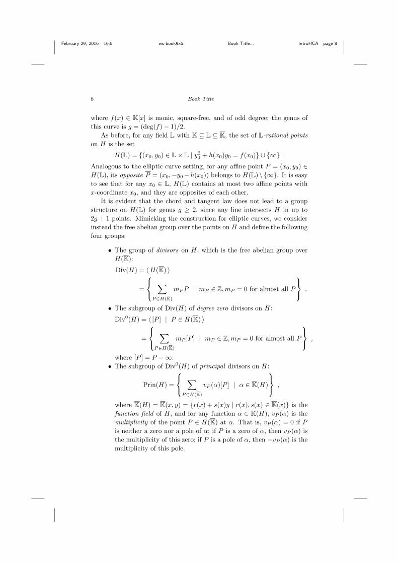
As before, for any field L with K ⊆ L ⊆ K, the set of L-rational points

on H is the set

H(L) = {(x0, y0) ∈ L× L | y20 + h(x0)y0 = f(x0)} ∪ {∞} .Analogous to the elliptic curve setting, for any affine point P = (x0, y0) ∈H(L), its opposite P = (x0,−y0−h(x0)) belongs to H(L) \ {∞}. It is easy

to see that for any x0 ∈ L, H(L) contains at most two affine points with

x-coordinate x0, and they are opposites of each other.

It is evident that the chord and tangent law does not lead to a group

structure on H(L) for genus g ≥ 2, since any line intersects H in up to

2g + 1 points. Mimicking the construction for elliptic curves, we consider

instead the free abelian group over the points on H and define the following

four groups:

• The group of divisors on H, which is the free abelian group over

H(K):

Div(H) = 〈H(K) 〉

=

∑P∈H(K)

mPP | mP ∈ Z,mP = 0 for almost all P

.

• The subgroup of Div(H) of degree zero divisors on H:

Div0(H) = 〈 [P ] | P ∈ H(K) 〉

=

∑P∈H(K)

mP [P ] | mP ∈ Z,mP = 0 for almost all P

,

where [P ] = P −∞.

• The subgroup of Div0(H) of principal divisors on H:

Prin(H) =

∑P∈H(K)

vP (α)[P ] | α ∈ K(H)

,

where K(H) = K(x, y) = {r(x) + s(x)y | r(x), s(x) ∈ K(x)} is the

function field of H, and for any function α ∈ K(H), vP (α) is the

multiplicity of the point P ∈ H(K) at α. That is, vP (α) = 0 if P

is neither a zero nor a pole of α; if P is a zero of α, then vP (α) is

the multiplicity of this zero; if P is a pole of α, then −vP (α) is the

multiplicity of this pole.



• The degree zero class group or Jacobian3 of H:

Jac(H) = Div0(H) /Prin(H) .

The Jacobian is the appropriate hyperelliptic curve generalization of the

group of points on an elliptic curve. The set of points on H embeds into

the Jacobian of H by assigning each P ∈ H(K) the coset of [P ] in Jac(H).

For elliptic curves, this embedding is in fact a group isomorphism, so the

point addition as defined in Section 1.2 is compatible with the group law

on the Jacobian of an elliptic curve. However, for hyperelliptic curves of

genus 2 and higher, this embedding is no longer surjective.

The identity in Jac(H) is the coset of [∞]. The generalization of the

elliptic curve motto that any three collinear points on E sum to zero is “all

the points on any function on H sum to zero”. That is, if P1, P2, . . . , Pr

is the complete collection of intersection points of H with some function

α ∈ K(H), with respective multiplicities vPi(α) for 1 ≤ i ≤ r, then the

divisor D =∑r

i=1 vPi(α)[Pi] is principal. Since for any affine point P =

(x0, y0) ∈ H(K), the line x = x0 intersects H only in P , P and ∞, we

see that the inverse of the class of [P ] is the class of −[P ] = [P ]. More

generally, the inverse of the class of a divisor D =∑mP [P ] in Jac(H) is

the class of D =∑mP [P ].

The (affine) support of a degree zero divisor D =∑mP [P ] ∈ Div0(H),

denoted supp(D), is the set of points P ∈ H(L) \ {∞} for which mP 6= 0.

The divisor D is semi-reduced if the following conditions are satisfied.

• mP > 0 for all P ∈ supp(D);

• If P ∈ supp(D) with P 6= P , then P /∈ supp(D);

• If P ∈ supp(D) with P = P , then mP = 1.

It is not hard to see that every class in Jac(H) contains a semi-reduced

divisor: simply replace every summand −[P ] by [P ], and subsequently re-

move all combinations of the form [P ] + [P ] = [∞] from D, noting that

2[P ] = [∞] when P = P .

A semi-reduced divisor D∑mP [P ] ∈ Div0(H) is reduced if

∑mP ≤ g,

where g is the genus of H. In particular, the support of a reduced divisor

contains at most g points. For example, the reduced divisors on a genus 2

hyperelliptic curve H are exactly the divisors of the form [P ] and [P ] + [Q]

with affine points P,Q ∈ H(K) such that Q 6= P . In fact, divisors of the3The Jacobian of an algebraic curve of genus g leads a double life as an abelian group

and a principally polarized abelian variety of dimension g called the Jacobian variety ofthe curve.


10 Book Title

form [P ] arising from affine points P on any hyperelliptic curve are always

reduced. The key enabler for efficient Jacobian arithmetic is the following

theorem, provable via Riemann-Roch theory:

Theorem 1.1. Every class in Jac(H) contains a unique reduced divisor.

The above theorem distills Jacobian arithmetic down to the following

question: given two reduced divisors D1 and D2, determine (efficiently) the

reduced representative of the class of D1 + D1 in Jac(H). We denote this

reduced representative by D1 ⊕D2.

1.4 Arithmetic on Reduced Divisors

To avoid clutter, we will frequently omit the square brackets in the de-

gree zero divisor notation and simply write semi-reduced divisors as sums

of affine points. We begin this section with an illustration of Jacobian

arithmetic via reduced divisors on a genus 2 example.

Example 1.1. Consider the genus 2 hyperelliptic curve H : y2 = f(x)

over Q with f(x) = x5 − 5x3 + 4x − 1. We wish to find D1 ⊕ D2 for

the two reduced divisors D1 = P1 + P2 and D2 = Q1 + Q2 on H, where

P1 = (−2, 1), P2 = (0, 1), Q1 = (2, 1) and Q2 = (3,−11). These four

points all lie on the unique degree 3 function y − v(x) ∈ Q(H) where

v(x) = −(4/5)x3 + (16/5)x + 1. The curve y = v(x) intersects H in two

more points R1 and R2. The x-coordinates of all six intersection points are

the roots of the equation

0 = f(x)− v(x)2 = −(x− (−2)

)(x− 0

)(x− 2

)(x− 3

)u(x)

with u(x) = 16x2 + 23x + 5. Thus, the x-coordinates of R1 and R2

are the zeros of u(x), and their y-coordinates are obtained by substitut-

ing their respective x-coordinates into y = v(x). Since the six points

P1, P2, Q1, Q2, R1, R2 form the complete intersection of H with y = v(x),

they sum to zero, so D1 ⊕D2 = R1 +R2, which is the divisor(−23 +

√209

32,

1333− 115√

209

2048

)+

(−23−

√209

32,

1333 + 115√

209

2048

)(1.5)

This process is illustrated in Figure 1.3.

In general, to find the reduced sum D1⊕D2 of two divisors D1 and D2

on a hyperelliptic curve (1.4), first determine the semi-reduced sum D of

D1 and D2; this is equal to the actual sum D1 +D2 unless P ∈ supp(D2)



Fig. 1.3 Divisor addition on H : y2 = x5 − 5x3 + 4x − 1 over Q (solid curve). Thefunction y = −(4/5)x3 + (16/5)x + 1 (dashed curve) through D1 = (−2, 1) + (0, 1)

(white lozenges) and D2 = (2, 1) + (3,−11) (black lozenges) intersects H in the third

reduced divisor D = R1 +R2 (white circles) whose points have respective x-coordinates(−23 ±

√209)/32 and y-coordinates (−1333 ± 115

√209)/2048. Hence D1 ⊕ D2 = D

(black circles).

-10

-5

0

5

10

-3 -2 -1 0 1 2 3

for some P ∈ supp(D1). Normally, D will not be reduced, and in fact

r = |supp(D)| can be as large as 2g. So assume that r ≥ g + 1, and iterate

over D as follows.

The r points in supp(D) all lie on an interpolation curve y = v(x) with

deg(v) ≤ r − 1. Substitute this curve into (1.4)) to obtain the polynomial

F (x) = f(x) − v(x)2 − h(x)v(x). Put d = deg(F ). Among the d zeros

of F (x) (counted with multiplicities), r are the x-coordinates of the points

in supp(D). Determine the remaining d− r zeros xi (1 ≤ i ≤ d− r) of F (x)

and substitute them into y = v(x) to define d − r new points (xi, v(xi))

on H. Replace the r points in supp(D) by the opposites (xi,−v(xi)−h(xi))

of these d − r new points. This defines a new semi-reduced divisor in the

divisor class of D1 + D2, again called D, with |supp(D)| = d − r. Now


12 Book Title

consider two cases:

Case 1 : d ≥ 2g + 2. Then the unique degree-dominant term in F (x) is

−v(x)2, so d− r = 2 deg(v)− r ≤ 2(r − 1)− r = r − 2.

Case 2 : d ≤ 2g + 1. Then deg(v) ≤ g and the unique degree-dominant

term in F (x) is f(x), so d− r = 2g + 1− r ≤ 2g + 1− (g + 1) = g. Thus,

D is reduced.

It follows that the number of points in supp(D) decreases by 2 in each

iteration of the reduction procedure, except possibly in the last reduction

step where it decreases by at least 1. Since r ≤ 2g at the beginning of

this process, the reduced divisor D1 ⊕D2 is obtained after at most dg/2eiterations. For genus g = 2, as in Example 1.1, one reduction step is

sufficient.

1.5 Mumford Representations

In reality, the reduction process above is impractical since the points of a di-

visor may have coordinates in an extension of the base field K. For example,

the reduced divisor D given by (1.5) has support over the quadratic exten-

sion L = Q(√

209) of Q. Note, however, that the two points in supp(D)

exhibit a symmetry; specifically, they are images of each other under the

Q-automorphism√

209 7→ −√

209 on L. For reasons of efficiency, it is ob-

viously desirable to carry out Jacobian arithmetic exclusively in the base

field K.

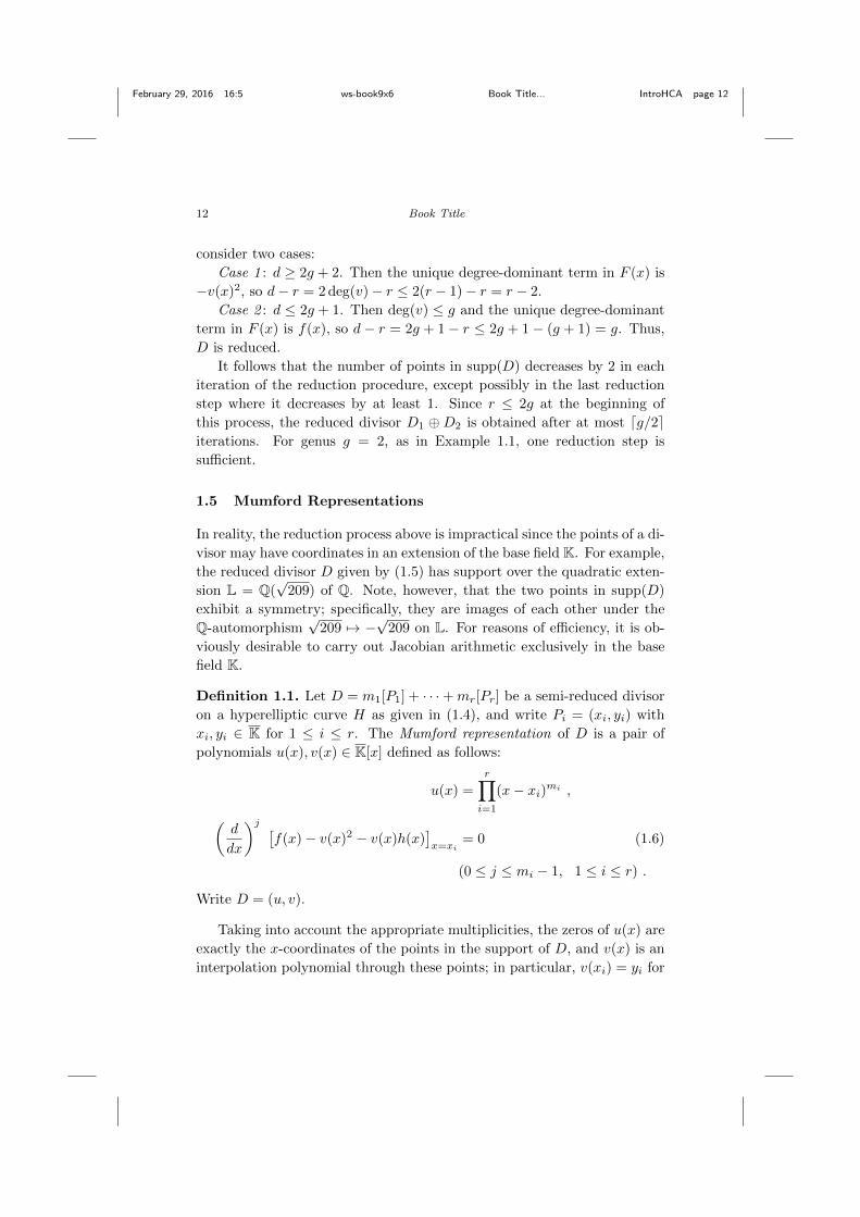
Definition 1.1. Let D = m1[P1] + · · ·+mr[Pr] be a semi-reduced divisor

on a hyperelliptic curve H as given in (1.4), and write Pi = (xi, yi) with

xi, yi ∈ K for 1 ≤ i ≤ r. The Mumford representation of D is a pair of

polynomials u(x), v(x) ∈ K[x] defined as follows:

u(x) =

r∏i=1

(x− xi)mi ,

(d

dx

)j [f(x)− v(x)2 − v(x)h(x)

]x=xi

= 0 (1.6)

(0 ≤ j ≤ mi − 1, 1 ≤ i ≤ r) .

Write D = (u, v).

Taking into account the appropriate multiplicities, the zeros of u(x) are

exactly the x-coordinates of the points in the support of D, and v(x) is an

interpolation polynomial through these points; in particular, v(xi) = yi for



1 ≤ i ≤ r. Note that u(x) is monic and divides f(x)−v(x)2−h(x)v(x). The

divisor D uniquely determines u(x) and v(x) mod u(x); conversely, any pair

of polynomials u(x), v(x) as defined in (1.6) defines a semi-reduced divisor

D =∑r

i=1mi[Pi], with Pi = (xi, v(xi)) for 1 ≤ i ≤ r, on the hyperelliptic

curve (1.4). To ensure uniqueness, we will always choose v(x) to be of least

non-negative degree in its congruence class modulo u(x). This means in

particular that if D = (u, v) is reduced, then deg(v) < deg(u) ≤ g.

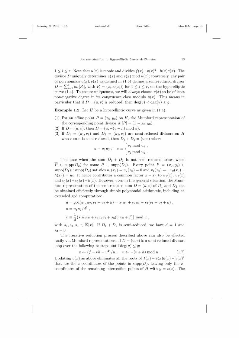
Example 1.2. Let H be a hyperelliptic curve as given in (1.4).

(1) For an affine point P = (x0, y0) on H, the Mumford representation of

the corresponding point divisor is [P ] = (x− x0, y0).

(2) If D = (u, v), then D = (u,−(v + h) mod u).

(3) If D1 = (u1, v1) and D2 = (u2, v2) are semi-reduced divisors on H

whose sum is semi-reduced, then D1 +D2 = (u, v) where

u = u1u2 , v ≡

{v1 mod u1 ,

v2 mod u2 .

The case when the sum D1 + D2 is not semi-reduced arises when

P ∈ supp(D2) for some P ∈ supp(D1). Every point P = (x0, y0) ∈supp(D1)∩supp(D2) satisfies u1(x0) = u2(x0) = 0 and v1(x0) = −v2(x0)−h(x0) = y0. It hence contributes a common factor x − x0 to u1(x), u2(x)

and v1(x)+v2(x)+h(x). However, even in this general situation, the Mum-

ford representation of the semi-reduced sum D = (u, v) of D1 and D2 can

be obtained efficiently through simple polynomial arithmetic, including an

extended gcd computation:

d = gcd(u1, u2, v1 + v2 + h) = s1u1 + s2u2 + s3(v1 + v2 + h) ,

u = u1u2/d2 ,

v ≡ 1

d

(s1u1v2 + s2u2v1 + s3(v1v2 + f)

)mod u ,

with s1, s2, s3 ∈ K[x]. If D1 + D2 is semi-reduced, we have d = 1 and

s3 = 0.

The iterative reduction process described above can also be effected

easily via Mumford representations. If D = (u, v) is a semi-reduced divisor,

loop over the following to steps until deg(u) ≤ g:

u← (f − vh− v2)/u , v ← −(v + h) mod u . (1.7)

Updating u(x) as above eliminates all the roots of f(x)− v(x)h(x)− v(x)2

that are the x-coordinates of the points in supp(D), leaving only the x-

coordinates of the remaining intersection points of H with y = v(x). The


14 Book Title

formula for v(x) in (1.7) replaces these intersections points by their oppo-

sites. The above process of divisor addition with subsequent reduction is

due to Cantor [9].

Example 1.3. The respective Mumford representations of the reduced di-

visors D1 and D2 of Example 1.1) are

D1 = (x2 + 2x, 1), D2 = (x2 − 5x+ 6,−12x+ 25) .

Thus, D1 +D2 = (u, v) where

u(x) = x4 − 3x3 − 4x2 + 12x , v(x) = −4

5x3 +

16

5x+ 1 .

The reader will recognize the polynomial v(x) from Example 1.1. One

reduction step (1.7) produces u(x) = 16x2 + 23x+ 5 (which the reader will

again recognize from Example 1.1) and v(x) = (16x − 23)/320, yielding

D1 ⊕D2 = (16x2 + 23x+ 5, (16x− 23)/320).

Note that the Mumford polynomials u(x) and v(x) of the divisorD1⊕D2

of Example 1.3 have coefficients in Q, whereas the points in its support

have coordinates in Q(√

209). This is no accident. For any hyperelliptic

curve H over K, every K-automorphism of the Galois group Gal(K/K) acts

on points on H coordinatewise (leaving ∞ fixed), and on divisors on H

pointwise. A divisor on H is defined over K if it is Gal(K/K)-invariant. In

other words, any Galois automorphism of K/K may permute the points

in the support of a divisor that is defined over K, but must leave the

entire divisor fixed. For example, the reduced divisor D given in (1.5)

is defined over Q, since every Q-automorphism of Q is either the identity

or the involution√

209 7→ −√

209 when restricted to L = Q(√

209). This

can also be seen from the following key theorem that can easily be proved

using Galois theory:

Theorem 1.2. A semi-reduced divisor D = (u, v) on a hyperelliptic

curve H over a field K is defined over K if and only if u(x) and v(x)

have coefficients in K.

Let JacK(H) denote the subgroup of Jac(H) of divisor classes repre-

sented by reduced divisors defined over K. Theorem 1.2, combined with

the algorithms presented above, guarantees that arithmetic in JacK(H) is

entirely effected through simple and efficient polynomial arithmetic in K[x].

Moreover, Theorems 1.1 and 1.2 establish that for a finite field K = Fq,

JacFq(H) is finite. This group therefore satisfies all the efficiency require-

ments for cryptographic applications.



1.6 Beyond Weierstraß Models

Many elliptic curves can be described by equations other than (1.1) that

may support faster point addition at the expense of the most general pos-

sible form. Edwards curves, for example, allow for very efficient point addi-

tion formulas which in addition are complete, i.e. exceptional cases such as

adding two opposite points or adding the infinite point to some point are

included in the formulas and need not be considered separately. Hessian

models can also be very effective for point arithmetic. For a comprehen-

sive overview of other elliptic curve models and their arithmetic, the reader

is referred to the Explicit-Formulas Database [4]. For some operations on

points, using other coordinate systems such as projective coordinates can

be advantageous; sometimes mixed coordinates, where the two input points

are given in different coordinate systems, are best.

The two aforementioned special models for elliptic curves unfortunately

do not extend to higher genus. However, appropriate variable transfor-

mations applied to (1.4) can remove some terms. The simplest of these

eliminates the coefficient c of x2g in f(x) when the characteristic of K does

not divide 2g + 1 by mapping x to x − c/(2g + 1); for elliptic curves, this

is precisely the isomorphism from (1.1) to (1.2). In a completely different

vein, there is a highly efficient arithmetic framework for genus 2 curves

that uses the Kummer surface associated to the curve, rather than its Ja-

cobian [17,19].

There are also even degree models for both elliptic and hyperelliptic

curves. They take the same form as (1.4), except that deg(f) = 2g + 2.

Moreover, when K has characteristic 2, then deg(h) = g+ 1, h(x) is monic,

and the leading coefficient of f(x) has the form s2+s for some s ∈ K\{0, 1}.Even degree curves are more general than their odd degree counterparts,

since every odd degree model can be converted to a K-isomorphic even

degree model. However, the reverse transformation requires a zero of f(x),

and in fact a common zero of f(x) and h(x) in characteristic 2, and thus

may only be defined over an extension field of K of degree up to 2g+ 2; see

Theorem 12.4.12, p. 448, of [33].

Investigating the homogenization of even degree hyperelliptic curve

models reveals that the projective point [0 : 1 : 0] is singular; the ob-

servant reader will note that this is in fact also the case for odd degree

hyperelliptic curves of genus g ≥ 2. To ascertain the behaviour at infinity

on these curves, put F (x, y) = y2 + h(x)y− f(x) and substitute x = 0 into

the isomorphic curve x2g+2F (x−1, yx−g−1) = 0. For odd genus (including


16 Book Title

genus 1), this yields y2 = 0 and thus the unique point (0, 0). For even degree

and characteristic different from 2, we obtain y2 = 1 and thus two distinct

points (0, 1) and (0,−1). Finally, for even degree and characteristic 2, we

get y2 + y = s2 + s, producing the two distinct points (0, s) and (0, s+ 1).

Thus, odd degree models have one infinite point, whereas even degree mod-

els have two infinite points that are opposites of each other. This extra

degree of freedom at infinity leads to complications for arithmetic on even

degree models. As a result, research on this subject is far less advanced

than investigations into the more traditional odd degree models.

Paulus and Ruck [34] found a unique representation of degree zero di-

visor classes on even degree hyperelliptic curves via reduced divisors with

a very small contribution (usually none) at one of the infinite points. Un-

fortunately, the group operation on these representatives is considerably

slower than that on odd degree models. Jacobian arithmetic can be sped

up considerably, to the point where it is close to competitive with odd degree

model arithmetic, by instead prescribing approximately equal contributions

at the two infinite points (so-called balanced divisors) [15].

Another natural approach is to define reduced divisors on an even de-

gree hyperelliptic curve H completely analogous to the odd degree scenario,

except that the unique infinite point on an odd degree model is replaced

by one of the two infinite points on H (with the other infinite point not

appearing in the divisor). The divisors thus obtained represent almost all

divisor classes — leaving out only a heuristically expected proportion of

1/q of them [21] — and form the infrastructure of H. Addition on the

infrastructure can be defined completely analogous to Jacobian arithmetic

on odd degree models by applying Cantor’s algorithm to the affine parts of

any two infrastructure divisors; note that this is is different from Jacobian

arithmetic on even degree models. Under this operation, the infrastruc-

ture is closed but not necessarily associative. The heuristically expected

proportion of infrastructure divisors that violate associativity is approx-

imately 1/q, the same as that of “missing” divisor classes. As a result,

infrastructures over large finite fields behave “almost” like abelian groups,

and can in fact serve as a suitable setting for discrete logarithm based

cryptography [23, 24], providing the same degree of security as the Jaco-

bian setting. Moreover, the infrastructure of H can be embedded into the

cyclic subgroup of JacK(H) generated by the divisor class of∞−∞, where

∞ and ∞ are the two infinite points on H [14].

For hyperelliptic curves of small genus, the algorithms on Mumford

polynomials can be realized symbolically as arithmetic on their coefficients



in the base field. Such explicit formulas were first presented for odd degree

models of genus 2 in [29], and the effort to optimize explicit field arithmetic

in this setting has spawned a considerable volume of literature too exten-

sive to cite here. Explicit formulas on odd degree models of genus 3 and 4

exist as well; first presented in [41], the genus 3 formulas in particular have

undergone much refinement. Explicit formulas for even degree models of

genus 2 can be found in [13]; work on even degree genus 3 curves is currently

in progress. For Jacobian arithmetic on (even and odd degree) hyperelliptic

curves of higher genus, the NUCOMP algorithm described in [25,40] signif-

icantly outperforms Cantor’s algorithm, especially for large genus and/or a

large finite base field [22]. Efficient realization of the Jacobian group law on

a number of families of non-hyperelliptic curves has also been investigated;

in the interest of space, we forego citing any sources here. All told, explicit

arithmetic and algorithms in Jacobians of curves and more generally, on

abelian varieties — which represent higher dimensional analogues of curves

— are the subject of intense ongoing research.

Acknowledgment The author is supported by a Discovery Grant from

the National Science and Engineering Research Council (NSERC) of

Canada. Thanks go to Gove Effinger, host and organizer of the Fq12 con-

ference, for inviting me to present this work at Fq12 and encouraging me to

write this article. Finally, the helpful comments of an anonymous reviewer

are appreciated.



Bibliography

[1] L. M. Adleman, J. DeMarrais amd M.-D. Huang, A subexponential algo-rithm for discrete logarithms over hyperelliptic curves of large genus overGF(q). Theoret. Comput. Sci. 226 (1999), no. 1-2, 7–18.

[2] R. Barbulescu, P. Gaudry, A. Joux and E. Thome, A heuristic quasi-polynomial algorithm for discrete logarithm in finite fields of small char-acteristic. Advances in Cryptology — EUROCRYPT 2014, 1–16, LectureNotes in Comput. Sci., 8441, Springer, Heidelberg, 2014.

[3] E. Barker, W. Barker, W. Polk, W. Burr and M. Smid, Recommendationfor key management – part 1: general (revision 3), NIST Special Publication800-57, July 2012.

[4] D. J. Bernstein and T. Lange, Explicit-Formulas Database, http://

hyperelliptic.org/EFD/.[5] J. W. Bos, C. Costello, H. Hisil, K. Lauter, Fast Cryptography in Genus 2,

Advances in Cryptology — EUROCRYPT 2013, 194–210, Lecture Notes inComp. Sci., 7881, Springer, Heidelberg, 2014.

[6] A. Bostan, P. Gaudry and E. Schost, Linear recurrences with polynomialcoefficients and application to integer factorization and Cartier-Manin oper-ator. SIAM J. Comput. 36 (2007), no. 6, 1777–1806.

[7] R. Broker, E. W. Howe, K. E. Lauter and P. Stevenhagen, Genus-2 curvesand Jacobians with a given number of points. LMS J. Comput. Math. 18(2015), no. 1, 170–197

[8] R. Broker and P. Stevenhagen, Elliptic curves with a given number of points.Algorithmic Number Theory, 117–131, Lecture Notes in Comput. Sci., 3076,Springer, Berlin, 2004.

[9] D. G. Cantor, Computing in the Jacobian of a hyperelliptic curve. Math.Comp. 48 (1987), no. 177, 95–101.

[10] H. Cohen, G. Frey, R. Avanzi, C. Doche, T. Lange, K. Nguyen, F. Ver-cauteren, Handbook of Elliptic and Hyperelliptic Curve Cryptography, Chap-man & Hall/CRC, Boca Raton, Florida, 2006.

[11] C. Diem, An index calculus algorithm for plane curves of small degree. Al-gorithmic Number Theory, 543–557, Lecture Notes in Comput. Sci., 4076,Springer, Berlin, 2006.

19

http://hyperelliptic.org/EFD/

http://hyperelliptic.org/EFD/


20 Book Title

[12] W. Diffie and M. E. Hellman, New directions in cryptography. IEEE Trans.Information Theory IT-22 (1976), no. 6, 644–654.

[13] S. Erickson, M.J. Jacobson, and A. Stein. Explicit formulas for real hyperel-liptic curves of genus 2 in affine representation. Adv. Math. Communication5 (2011), no. 4, 623–666.

[14] F. Fontein, The infrastructure of a global field of arbitrary unit rank. Math.Comp. 80 (2011), no. 276, 2325–2357.

[15] S. D. Galbraith, M. Harrison and D. J. Mireles Morales, Efficient hyper-elliptic arithmetic using balanced representation for divisors. AlgorithmicNumber Theory, 342–356, Lecture Notes in Comput. Sci., 5011, Springer,Berlin, 2008.

[16] P. Gaudry, An algorithm for solving the discrete log problem on hyperellip-tic curves. Advances in Cryptology — EUROCRYPT 2000 (Bruges), 19–34,Lecture Notes in Comput. Sci., 1807, Springer, Berlin, 2000.

[17] P. Gaudry, Fast genus 2 arithmetic based on theta functions. J. Math. Cryp-tol. 1 (2007), no. 3, 243–265.

[18] P. Gaudry and R. Harley, Counting points on hyperelliptic curves over finitefields. Algorithmic number theory (Leiden, 2000), 313–332, Lecture Notes inComput. Sci., 1838, Springer, Berlin, 2000.

[19] P. Gaudry and D. Lubicz, The arithmetic of characteristic 2 Kummer sur-faces and of elliptic Kummer lines. Finite Fields Appl. 15 (2009), no. 2,246–260.

[20] D. M. Gordon, Discrete logarithms in GF(p) using the number field sieve.SIAM J. Discrete Math. 6 (1993), no. 1, 124–138.

[21] M. J. Jacobson, Jr., M. Rezai Rad and R. Scheidler, Comparison of scalarmultiplication on real hyperelliptic curves. Adv. Math. Communications 8(2014), no. 4, 389–406.

[22] M. J. Jacobson, Jr., R. Scheidler and A. Stein, Fast arithmetic on hyperel-liptic curves via continued fraction expansions. Advances in Coding Theoryand Cryptology, 200–243, Ser. Coding Theory Cryptol., 3, World ScientificPublishing Co. Pte. Ltd., Hackensack, New Jersey 2007.

[23] M. J. Jacobson, Jr., R. Scheidler and A. Stein, Cryptographic protocolson real hyperelliptic curves. Adv. Math. Communications 1 (2007), no. 2,197–221.

[24] M. J. Jacobson, Jr., R. Scheidler and A. Stein, Cryptographic aspects of realhyperelliptic curves. Tatra Mountains Math. Pub. 47 (2010), no. 1, 31–65.

[25] M. J. Jacobson, Jr. and A. J. van der Poorten, Computational aspects ofNUCOMP, Algorithmic Number Theory (Sydney, 2002), 120–133, LectureNotes in Comput. Sci., 2369, Springer, Berlin, 2002.

[26] A. Joux, A new index-calculus algorithm with complexity L(1/4 + o(1))in very small characteristic. Selected Areas in Cryptography — SAC 2013,355–379, Lecture Notes in Comp. Sci., 8282, Springer, Berlin 2014.

[27] K. S. Kedlaya, Counting points on hyperelliptic curves using Monsky-Washnitzer cohomology. J. Ramanujan Math. Soc. 16 (2001), no. 4, 323–338.

[28] N. Koblitz, Elliptic curve cryptosystems. Math. Comp. 48 (1987), no. 177,203–209.


Bibliography 21

[29] T. Lange, Formulae for Arithmetic on Genus 2 Hyperelliptic Curves. Ap-plicable Algebra in Engineering, Communication and Computing 15 (2005),no. 5, 295–328.

[30] A. Lauder and D. Wan, Computing zeta functions of Artin-Schreier curvesover finite fields. LMS J. Comput. Math. 5 (2002), 34–55.

[31] V. S. Miller, Use of elliptic curves in cryptography. Advances in Cryptology— CRYPTO ’85 (Santa Barbara, Calif., 1985), 417–426, Lecture Notes inComput. Sci., 218, Springer, Berlin, 1986.

[32] V. Muller, A. Stein and C. Thiel, Computing discrete logarithms in realquadratic congruence function fields of large genus. Math. Comp. 68 (1999),no. 226, 807–822.

[33] G. L. Mullen and D. Panario (eds.), Handbook of Finite Fields.. DiscreteMathematics and its Applications, CRC Press, Boca Raton, Florida, 2013.

[34] S. Paulus and H.-G. Ruck, Real and imaginary quadratic representations ofhyperelliptic function fields. Math. Comp. 68 (1999), no. 227, 1233–1241.

[35] S. C. Pohlig and M. Hellman, An improved algorithm for computing loga-rithms over GF(p) and its cryptographic significance. IEEE Trans. Informa-tion Theory IT-24 (1978), no. 1, 106–110.

[36] J. M. Pollard, A Monte Carlo method for factorization. Nordisk Tidskr.Informationsbehandlung (BIT) 5 (1975), no. 3, 331–334.

[37] D. Shanks, Class number, a theory of factorization, and genera. 1969 NumberTheory Institute (Proc. Sympos. Pure Math., Vol. XX, State Univ. New York,Stony Brook, N.Y., 1969), pp. 415–440. Amer. Math. Soc., Providence, R.I.,1971.

[38] V. Shoup, Lower bounds for discrete logarithms and related problems. Ad-vances in Cryptology — EUROCRYPT ’97 (Konstanz), 256–266, LectureNotes in Comput. Sci., 1233, Springer, Berlin, 1997.

[39] N. Theriault, Index calculus attack for hyperelliptic curves of small genus.Advances in Cryptology — ASIACRYPT 2003, 75–92, Lecture Notes inComput. Sci., 2894, Springer, Berlin, 2003.

[40] A. van der Poortem, A note om NUCOMP, Math. Comp. 72 (2003), no.244, 1935–1946

[41] T. Wollinger, Software and Hardware Implementation of HyperellipticCurve Cryptosystems. Doctoral Dissertation, Ruhr-Universitat Bochum(Germany), 2004.

Documents

An Introduction to Hyperelliptic Curve Arithmeticpeople.ucalgary.ca/~rscheidl/Papers/IntroHCA.pdf · IntroHCA page 1 Chapter 1 An Introduction to Hyperelliptic Curve Arithmetic