Embed Size (px)
Citation preview

1
© Duraiswami & Gumerov, 2003-2004CSCAMM FAM04: 04/19/2004
An Introduction to Fast Multipole Methods
Ramani DuraiswamiInstitute for Advanced Computer Studies
University of Maryland, College Parkhttp://www.umiacs.umd.edu/~ramani
Joint work with Nail A. Gumerov© Duraiswami & Gumerov, 2003-2004CSCAMM FAM04: 04/19/2004
Fast Multipole Methods• Computational simulation is becoming an accepted paradigm for
scientific discovery. Many simulations involve several million variables
• Most large problems boil down to solution of linear system or performing a matrix-vector product
• Regular product requires O(N2) time and O(N2) memory• The FMM is a way to
accelerate the products of particular dense matrices with vectorsDo this using O(N) memory
• FMM achieves product in O(N) or O(N log N) time and memory• Combined with iterative solution methods, can allow solution of
problems hitherto unsolvable
© Duraiswami & Gumerov, 2003-2004CSCAMM FAM04: 04/19/2004
Matrix vector product
s1 = m11 x1 + m12 x2 + … + m1d xd
s2 = m21 x1 + m22 x2 + … + m2d xd
…sn = mn1 x1 + mn2 x2 + … + mnd xd
• d products and sums per line
• N lines• Total Nd products
and Nd sums to calculate N entries
• Memory needed is NM entries
• Matrix vector product is identical to a sum
si = ∑j=1d mij xj
• So algorithm for fast matrix vector products is also a fast summation algorithm
© Duraiswami & Gumerov, 2003-2004CSCAMM FAM04: 04/19/2004
Linear Systems• Solve a system of equations
Mx=s• M is a N × N matrix, x is a N vector, s is a N vector
• Direct solution (Gauss elimination, LU Decomposition, SVD, …) all need O(N3) operations
• Iterative methods typically converge in k steps with each step needing a matrix vector multiply O(N2)
if properly designed, k<< N
• A fast matrix vector multiplication algorithm requiring O(N log N) operations will speed all these algorithms
Tutorial Lectures on the Fast Multipole Method [email protected]@umiacs.umd.edu
Presented at the Center for Scientific Computing and Mathematical Modeling, University of Maryland, College ParkCopyright, Nail A. Gumerov and Ramani Duraiswami, 2002-2004.

2
© Duraiswami & Gumerov, 2003-2004CSCAMM FAM04: 04/19/2004
Is this important?• Argument:
Moore’s law: Processor speed doubles every 18 monthsIf we wait long enough the computer will get fast enough and let my inefficient algorithm tackle the problem
• Is this true?Yes for algorithms with same asymptotic complexityNo!! For algorithms with different asymptotic complexity
• For a million variables, we would need about 16 generations of Moore’s law before a O(N2) algorithm is comparable with a O(N) algorithm
• Similarly, clever problem formulation can also achieve large savings.
© Duraiswami & Gumerov, 2003-2004CSCAMM FAM04: 04/19/2004
Memory complexity
• Sometimes we are not able to fit a problem in available memory
Don’t care how long solution takes, just if we can solve it • To store a N × N matrix we need N2 locations
1 GB RAM = 10243 =1,073,741,824 bytes=> largest N is 32,768
• “Out of core” algorithms copy partial results to disk, and keep only necessary part of the matrix in memory
Extremely slow
• FMM allows reduction of memory complexity as wellElements of the matrix required for the product can be generated as neededCan solve much larger problems (e.g., 107 variables on a PC)
© Duraiswami & Gumerov, 2003-2004CSCAMM FAM04: 04/19/2004
The need for fast algorithms• Grand challenge problems in large numbers of variables • Simulation of physical systems
Electromagnetics of complex systemsStellar clustersProtein foldingAcousticsTurbulence
• Learning theoryKernel methods Support Vector Machines
• Graphics and VisionLight scattering …
© Duraiswami & Gumerov, 2003-2004CSCAMM FAM04: 04/19/2004
• General problems in these areas can be posed in terms of millions (106) or billions (109) of variables
• Recall Avogadro’s number (6.022 141 99 × 1023
molecules/mole• Job of modeling is to find symmetries and representations
that reduce the size of the problem• Even after state of art modeling, problem size may be
large
Tutorial Lectures on the Fast Multipole Method [email protected]@umiacs.umd.edu
Presented at the Center for Scientific Computing and Mathematical Modeling, University of Maryland, College ParkCopyright, Nail A. Gumerov and Ramani Duraiswami, 2002-2004.

3
© Duraiswami & Gumerov, 2003-2004CSCAMM FAM04: 04/19/2004
Dense and Sparse matrices• Operation estimates are for dense matrices.
Majority of elements of the matrix are non-zero
• However in many applications matrices are sparse• A sparse matrix (or vector, or array) is one in which most
of the elements are zero. If storage space is more important than access speed, it may be preferable to store a sparse matrix as a list of (index, value) pairs.For a given sparsity structure it may be possible to define a fast matrix-vector product/linear system algorithm
© Duraiswami & Gumerov, 2003-2004CSCAMM FAM04: 04/19/2004
• Can compute
In 5 operations instead of 25 operations• Sparse matrices are not our concern here
a1 0 0 0 00 a2 0 0 00 0 a3 0 00 0 0 a4 00 0 0 0 a5
x1
x2
x3
x4
x5
=
a1x1
a2x2
a3x3
a4x4
a5x5
© Duraiswami & Gumerov, 2003-2004CSCAMM FAM04: 04/19/2004
Structured matrices• Fast algorithms have been found for many dense matrices• Typically the matrices have some “structure”• Definition:
A dense matrix of order N × N is called structured if its entries depend on only O(N) parameters.
• Most famous example – the fast Fourier transform
© Duraiswami & Gumerov, 2003-2004CSCAMM FAM04: 04/19/2004
Fourier Matrices
FFT presented by Cooley and Tukey in 1965, but invented several times, including by Gauss (1809) and Danielson & Lanczos (1948)
Tutorial Lectures on the Fast Multipole Method [email protected]@umiacs.umd.edu
Presented at the Center for Scientific Computing and Mathematical Modeling, University of Maryland, College ParkCopyright, Nail A. Gumerov and Ramani Duraiswami, 2002-2004.

4
© Duraiswami & Gumerov, 2003-2004CSCAMM FAM04: 04/19/2004
FFT and IFFT
The FFT has revolutionized many applications by reducing the complexity by a factor of almost n
Can relate many other matrices to the Fourier Matrix
The discrete Fourier transform of a vector x is
the product Fnx.
The inverse discrete Fourier transform of a
vector x is the product F∗nx.
Both products can be done efficiently using the
fast Fourier transform (FFT) and the inverse
fast Fourier transform (IFFT) inO(n logn) time.
© Duraiswami & Gumerov, 2003-2004CSCAMM FAM04: 04/19/2004
Circulant Matrices
Toeplitz Matrices
Hankel Matrices
Vandermonde Matrices
© Duraiswami & Gumerov, 2003-2004CSCAMM FAM04: 04/19/2004
Structured Matrices• (usually) these matrices can be diagonalized by the
Fourier matrix• Product of diagonal matrix and vector requires O(N)
operations• So complexity is the cost of FFT (O (N log N)) + product
(O(N))• Order notation
Only keep leading order term (asymptotically important)So complexity of the above is O (N log N)
• Structured Matrix algorithms are “brittle”FFT requires uniform samplingSlight departure from uniformity breaks factorization
© Duraiswami & Gumerov, 2003-2004CSCAMM FAM04: 04/19/2004
• Introduced by Rokhlin & Greengard in 1987• Called one of the 10 most significant advances in computing of the
20th century• Speeds up matrix-vector products (sums) of a particular type
• Above sum requires O(MN) operations.• For a given precision ε the FMM achieves the evaluation in O(M+N)
operations.• Edelman: “FMM is all about adding functions”
Talk on Tuesday, next week
Fast Multipole Methods (FMM)
Tutorial Lectures on the Fast Multipole Method [email protected]@umiacs.umd.edu
Presented at the Center for Scientific Computing and Mathematical Modeling, University of Maryland, College ParkCopyright, Nail A. Gumerov and Ramani Duraiswami, 2002-2004.

5
© Duraiswami & Gumerov, 2003-2004CSCAMM FAM04: 04/19/2004
• FFT and other algorithms work on structured matrices• What about FMM ?• Speeds up matrix-vector products (sums) of a particular type
• Above sum also depends on O(N) parameters xi , yj, φ• FMM can be thought of as working on “loosely” structured matrices
Is the FMM a structured matrix algorithm?
© Duraiswami & Gumerov, 2003-2004CSCAMM FAM04: 04/19/2004
• Can accelerate matrix vector products Convert O(N2) to O(N log N)
• However, can also accelerate linear system solutionConvert O(N3) to O(kN log N)For some iterative schemes can guarantee k ≤ N
In general, goal of research in iterative methods is to reduce value of kWell designed iterative methods can converge in very few stepsActive research area: design iterative methods for the FMM
© Duraiswami & Gumerov, 2003-2004CSCAMM FAM04: 04/19/2004
A very simple algorithm• Not FMM, but has some key ideas• Consider
S(xi)=∑j=1N αj (xi – yj)2 i=1, … ,M
• Naïve way to evaluate the sum will require MN operations• Instead can write the sum as
S(xi)=(∑j=1N αj )xi
2 + (∑j=1N αjyj
2) -2xi(∑j=1N αjyj )
Can evaluate each bracketed sum over j and evaluate an expression of the type
S(xi)=β xi2 + γ -2xiδ
Requires O(M+N) operations
• Key idea – use of analytical manipulation of series to achieve faster summation
• May not always be possible to simply factorize matrix entries
© Duraiswami & Gumerov, 2003-2004CSCAMM FAM04: 04/19/2004
Approximate evaluation• FMM introduces another key idea or “philosophy”
In scientific computing we almost never seek exact answersAt best, “exact” means to “machine precision”
• So instead of solving the problem we can solve a “nearby” problem that gives “almost” the same answer
If this “nearby” problem is much easier to solve, and we can bound the error analytically we are done.
• In the case of the FMMExpress functions in some appropriate functional space with a given basisManipulate series to achieve approximate evaluationUse analytical expression to bound the error
• FFT is exact … FMM can be arbitrarily accurate
Tutorial Lectures on the Fast Multipole Method [email protected]@umiacs.umd.edu
Presented at the Center for Scientific Computing and Mathematical Modeling, University of Maryland, College ParkCopyright, Nail A. Gumerov and Ramani Duraiswami, 2002-2004.

6
© Duraiswami & Gumerov, 2003-2004CSCAMM FAM04: 04/19/2004
Approximation Algorithms• Computer science approximation algorithms
Approximation algorithms are usually directed at reducing complexity of exponential algorithms by performing approximate computationsHere the goal is to reduce polynomial complexity to linear orderConnections between FMM and CS approximation algorithms are not much explored
© Duraiswami & Gumerov, 2003-2004CSCAMM FAM04: 04/19/2004
Tree Codes• Idea of approximately evaluating matrix vector products
preceded FMM• Tree codes (Barnes and Hut, 1986)• Divides domain into regions and use approximate
representations• Key difference: lack error bounds, and automatic ways of
adjusting representations• Perceived to be easier to program
© Duraiswami & Gumerov, 2003-2004CSCAMM FAM04: 04/19/2004
Complexity• The most common complexities are
O(1) - not proportional to any variable number, i.e. a fixed/constant amount of timeO(N) - proportional to the size of N (this includes a loop to N and loops to
constant multiples of N such as 0.5N, 2N, 2000N - no matter what that is, if you double N you expect (on average) the program to take twice as long)O(N^2) - proportional to N squared (you double N, you expect it to take
four times longer - usually two nested loops both dependent on N).O(log N) - this is tricker to show - usually the result of binary splitting. O(N log N) this is usually caused by doing log N splits but also doing N
amount of work at each "layer" of splitting.
Exponential O(aN) : grows faster than any power of N
© Duraiswami & Gumerov, 2003-2004CSCAMM FAM04: 04/19/2004
Some FMM algorithms• Molecular and stellar dynamics
Computation of force fields and dynamics
• Interpolation with Radial Basis Functions• Solution of acoustical scattering problems
Helmholtz Equation
• Electromagnetic Wave scatteringMaxwell’s equations
• Fluid Mechanics: Potential flow, vortex flowLaplace/Poisson equations
• Fast nonuniform Fourier transform
Tutorial Lectures on the Fast Multipole Method [email protected]@umiacs.umd.edu
Presented at the Center for Scientific Computing and Mathematical Modeling, University of Maryland, College ParkCopyright, Nail A. Gumerov and Ramani Duraiswami, 2002-2004.

7
© Duraiswami & Gumerov, 2003-2004CSCAMM FAM04: 04/19/2004
Integral Equation• FMM is often used in integral equations• What is an integral equation?
• Function k(x,y) is called the kernel• Integral equations are typically solved by “quadrature”
Quadrature is the process of approximately evaluating an integral
• If we can write
© Duraiswami & Gumerov, 2003-2004CSCAMM FAM04: 04/19/2004
FMM-able Matrices
© Duraiswami & Gumerov, 2003-2004CSCAMM FAM04: 04/19/2004
FactorizationDegenerate Kernel:
O(pN) operations:
O(pM) operations:
Total Complexity: O(p(N+M))© Duraiswami & Gumerov, 2003-2004CSCAMM FAM04: 04/19/2004
“Middleman” Algorithm
SourcesSources
EvaluationPoints
EvaluationPoints
Standard algorithm Middleman algorithm
N M N M
Total number of operations: O(NM) Total number of operations: O(N+M)
Tutorial Lectures on the Fast Multipole Method [email protected]@umiacs.umd.edu
Presented at the Center for Scientific Computing and Mathematical Modeling, University of Maryland, College ParkCopyright, Nail A. Gumerov and Ramani Duraiswami, 2002-2004.

8
© Duraiswami & Gumerov, 2003-2004CSCAMM FAM04: 04/19/2004
Factorization
Non-Degenerate Kernel:
Error Bound:
Middleman Algorithm Applicability:
Truncation Number
© Duraiswami & Gumerov, 2003-2004CSCAMM FAM04: 04/19/2004
Factorization Problem:
•Usually there is no factorization available that provides a uniform approximation of the kernel in the entire computational domain.•So we have to construct a patchwork-quilt of overlapping approximations, and manage this.
•Need representations of functions that allow this•Need data structures for the management
© Duraiswami & Gumerov, 2003-2004CSCAMM FAM04: 04/19/2004
Five Key Stones of FMM
• Representation and Factorization• Error Bounds and Truncation• Translation• Space Partitioning• Data Structures
© Duraiswami & Gumerov, 2003-2004CSCAMM FAM04: 04/19/2004
Fast Multipole Methods
• Middleman (separation of variables) No space partitioning
• Single Level Methods Simple space partitioning (usually boxes)
• Multilevel FMM (MLFMM)Multiple levels of space partitioning (usually hierarchical boxes)
• Adaptive MLFMMData dependent space partitioning
Tutorial Lectures on the Fast Multipole Method [email protected]@umiacs.umd.edu
Presented at the Center for Scientific Computing and Mathematical Modeling, University of Maryland, College ParkCopyright, Nail A. Gumerov and Ramani Duraiswami, 2002-2004.

9
© Duraiswami & Gumerov, 2003-2004CSCAMM FAM04: 04/19/2004
Examples of Matrices
exp
© Duraiswami & Gumerov, 2003-2004CSCAMM FAM04: 04/19/2004
Iterative Methods
• To solve linear systems of equations;• Simple iteration methods;• Conjugate gradient or similar methods;• We use Krylov subspace methods:
Parameters of the method;Preconditioners;Research is ongoing.
• Efficiency critically depends on efficiency of the matrix-vector multiplication.
© Duraiswami & Gumerov, 2003-2004CSCAMM FAM04: 04/19/2004
Far and Near Field Expansions
xi
Ω
Ω
x*
R Sy
y
rc|xi - x*|
Rc|xi - x*|
xi
Ω
ΩΩ
x*
R Sy
y
rc|xi - x*|
Rc|xi - x*|
Far Field
Near Field
Far Field:
Near Field:
S: “Singular”(also “Multipole”,
“Outer”“Far Field”),
R: “Regular”(also “Local”,
“Inner”“Near Field”)
© Duraiswami & Gumerov, 2003-2004CSCAMM FAM04: 04/19/2004
Example of Multipole and Local expansions (3D Laplace)
Spherical Harmonics:x
y
z
O
x
y
z
O
x
y
z
Oθ
φ
r
r
Spherical Coordinates:
Tutorial Lectures on the Fast Multipole Method [email protected]@umiacs.umd.edu
Presented at the Center for Scientific Computing and Mathematical Modeling, University of Maryland, College ParkCopyright, Nail A. Gumerov and Ramani Duraiswami, 2002-2004.

10
© Duraiswami & Gumerov, 2003-2004CSCAMM FAM04: 04/19/2004
Idea of a Single Level FMM
Sources SourcesEvaluation
PointsEvaluation
Points
Standard algorithm SLFMM
N M N M
Total number of operations: O(NM) Total number of operations: O(N+M+KL)
K groupsL groups
Needs Translation!
© Duraiswami & Gumerov, 2003-2004CSCAMM FAM04: 04/19/2004
Multipole-to-Local S|R-translationAlso “Far-to-Local”, “Outer-to-Inner”, “Multipole-to-Local”
xi
Ω1i
Ω1i
Ω2i
x*1
x*2
S
(S|R)
y
R
Rc|xi - x*1|
R2 = min|x*2 - x*1|-Rc |xi - x*1|,rc|xi - x*2|
R2
xi
Ω1i
Ω1iΩ1i
Ω2i
x*1
x*2
S
(S|R)
y
R
Rc|xi - x*1|
R2 = min|x*2 - x*1|-Rc |xi - x*1|,rc|xi - x*2|
R2
© Duraiswami & Gumerov, 2003-2004CSCAMM FAM04: 04/19/2004
S|R-translation Operator
S|R-Translation Matrix
S|R-Translation Coefficients
© Duraiswami & Gumerov, 2003-2004CSCAMM FAM04: 04/19/2004
S|R-translation Operatorsfor 3D Laplace and Helmholtz equations
Tutorial Lectures on the Fast Multipole Method [email protected]@umiacs.umd.edu
Presented at the Center for Scientific Computing and Mathematical Modeling, University of Maryland, College ParkCopyright, Nail A. Gumerov and Ramani Duraiswami, 2002-2004.
11
© Duraiswami & Gumerov, 2003-2004CSCAMM FAM04: 04/19/2004
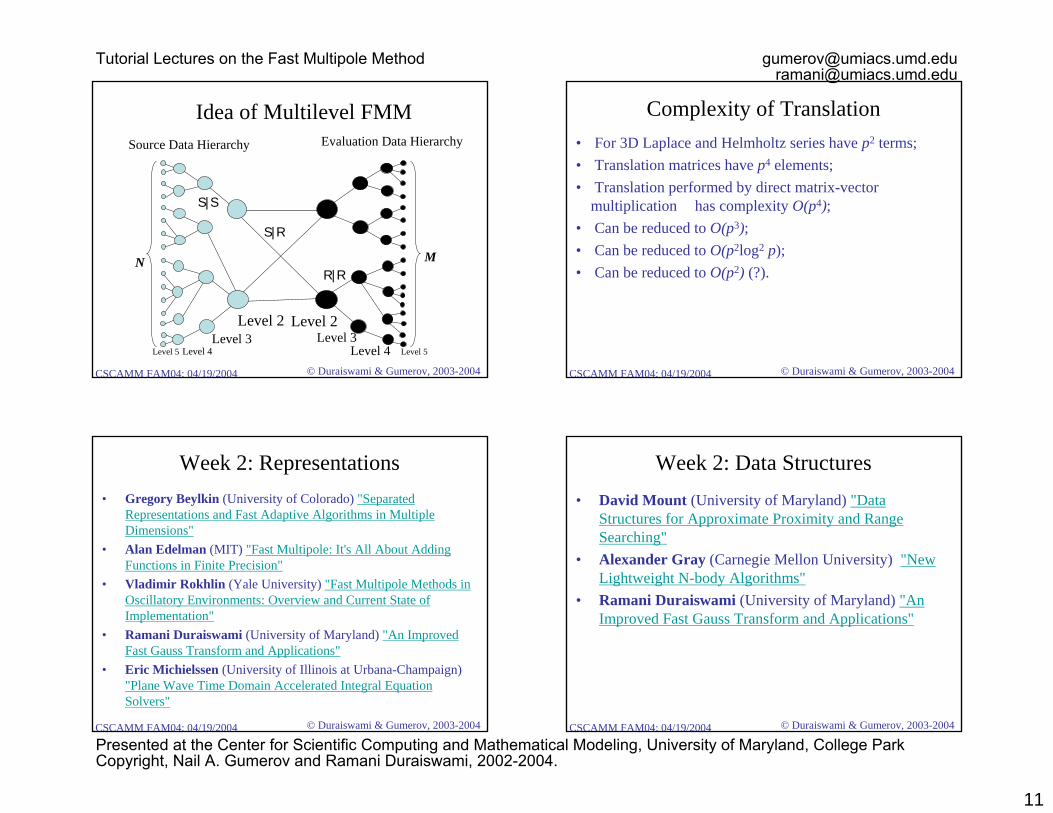
Idea of Multilevel FMMSource Data Hierarchy Evaluation Data Hierarchy
N M
Level 2Level 3
Level 4Level 5
Level 2Level 3
Level 4 Level 5
S|S
S|R
R|R
© Duraiswami & Gumerov, 2003-2004CSCAMM FAM04: 04/19/2004
Complexity of Translation• For 3D Laplace and Helmholtz series have p2 terms;• Translation matrices have p4 elements;• Translation performed by direct matrix-vector
multiplication has complexity O(p4);• Can be reduced to O(p3);• Can be reduced to O(p2log2 p);• Can be reduced to O(p2) (?).
© Duraiswami & Gumerov, 2003-2004CSCAMM FAM04: 04/19/2004
Week 2: Representations• Gregory Beylkin (University of Colorado) "Separated
Representations and Fast Adaptive Algorithms in Multiple Dimensions"
• Alan Edelman (MIT) "Fast Multipole: It's All About Adding Functions in Finite Precision"
• Vladimir Rokhlin (Yale University) "Fast Multipole Methods in Oscillatory Environments: Overview and Current State of Implementation"
• Ramani Duraiswami (University of Maryland) "An Improved Fast Gauss Transform and Applications"
• Eric Michielssen (University of Illinois at Urbana-Champaign) "Plane Wave Time Domain Accelerated Integral Equation Solvers"
© Duraiswami & Gumerov, 2003-2004CSCAMM FAM04: 04/19/2004
Week 2: Data Structures• David Mount (University of Maryland) "Data
Structures for Approximate Proximity and Range Searching"
• Alexander Gray (Carnegie Mellon University) "New Lightweight N-body Algorithms"
• Ramani Duraiswami (University of Maryland) "An Improved Fast Gauss Transform and Applications"
Tutorial Lectures on the Fast Multipole Method [email protected]@umiacs.umd.edu
Presented at the Center for Scientific Computing and Mathematical Modeling, University of Maryland, College ParkCopyright, Nail A. Gumerov and Ramani Duraiswami, 2002-2004.
12
© Duraiswami & Gumerov, 2003-2004CSCAMM FAM04: 04/19/2004
Week 2: Applications• Nail Gumerov (University of Maryland) "Computation of 3D Scattering from Clusters
of Spheres using the Fast Multipole Method"• Weng Chew (University of Illinois at Urbana-Champaign) "Review of Some Fast
Algorithms for Electromagnetic Scattering"• Leslie Greengard (Courant Institute, NYU) "FMM Libraries for Computational
Electromagnetics"• Qing Liu (Duke University) "NUFFT, Discontinuous Fast Fourier Transform, and
Some Applications"• Eric Michielssen (University of Illinois at Urbana-Champaign) "Plane Wave Time
Domain Accelerated Integral Equation Solvers"• Gregory Rodin (University of Texas, Austin) "Periodic Conduction Problems: Fast
Multipole Method and Convergence of Integral Equations and Lattice Sums"• Stephen Wandzura (Hughes Research Laboratories) "Fast Methods for Fast
Computers"• Toru Takahashi (Institue of Physical and Chemical Research (RIKEN), Japan) "Fast
Computing of Boundary Integral Equation Method by a Special-purpose Computer"• Ramani Duraiswami (University of Maryland) "An Improved Fast Gauss Transform
and Applications"
© Duraiswami & Gumerov, 2003-2004CSCAMM FAM04: 04/19/2004
Tree Codes:• Atsushi Kawai (Saitama Institute of Technology) "Fast
Algorithms on GRAPE Special-Purpose Computers"• Walter Dehnen (University of Leicester) "falcON: A
Cartesian FMM for the Low-Accuracy Regime"• Robert Krasny (University of Michigan) "A Treecode
Algorithm for Regularized Particle Interactions“• Derek Richardson (University of Maryland)
"pkdgrav: A Parallel k-D Tree Gravity Solver for N-Body Problems"
© Duraiswami & Gumerov, 2003-2004CSCAMM FAM04: 04/19/2004
Key Ideas of the FMM
Nail Gumerov & Ramani Duraiswami
UMIACS[gumerov][ramani]@umiacs.umd.edu
© Duraiswami & Gumerov, 2003-2004CSCAMM FAM04: 04/19/2004
Content• Summation Problems• Factorization (Middleman Method)• Space Partitioning (Modified Middleman Method)• Translations (Single Level FMM)• Hierarchical Space Partitioning (Multilevel FMM)
Tutorial Lectures on the Fast Multipole Method [email protected]@umiacs.umd.edu
Presented at the Center for Scientific Computing and Mathematical Modeling, University of Maryland, College ParkCopyright, Nail A. Gumerov and Ramani Duraiswami, 2002-2004.

13
© Duraiswami & Gumerov, 2003-2004CSCAMM FAM04: 04/19/2004
Summation Problems
© Duraiswami & Gumerov, 2003-2004CSCAMM FAM04: 04/19/2004
Matrix-Vector Multiplication
© Duraiswami & Gumerov, 2003-2004CSCAMM FAM04: 04/19/2004
Why Rd ?• d = 1
Scalar functions, interpolation, etc.• d = 2,3
Physical problems in 2 and 3 dimensional space• d = 4
3D Space + time, 3D grayscale images• d = 5
Color 2D images, Motion of 3D grayscale images• d = 6
Color 3D images• d = 7
Motion of 3D color images• d = arbitrary
d-parametric spaces, statistics, database search procedures
© Duraiswami & Gumerov, 2003-2004CSCAMM FAM04: 04/19/2004
Fields (Potentials)
Field (Potential) of a single(ith) unit source
Field (Potential) of the setof sources of intensities ui
Fields are continuous! (Almost everywhere)
Tutorial Lectures on the Fast Multipole Method [email protected]@umiacs.umd.edu
Presented at the Center for Scientific Computing and Mathematical Modeling, University of Maryland, College ParkCopyright, Nail A. Gumerov and Ramani Duraiswami, 2002-2004.

14
© Duraiswami & Gumerov, 2003-2004CSCAMM FAM04: 04/19/2004
Examples of Fields• There can be vector or scalar fields (we focus mostly on scalar fields)• Fields can be regular or singular
(singular at y = xi)
(singular at y = xi)
(regular everywhere)
Scalar Fields:
Vector Field:
(singular at y = xi)© Duraiswami & Gumerov, 2003-2004CSCAMM FAM04: 04/19/2004
Straightforward Computational Complexity:
O(MN) Error: 0 (“machine” precision)
The Fast Multipole Methods look for computation of the same problemwith complexity o(MN) and error < prescribed error.
In the case when the error of the FMM does not exceed the machine precision error (for given number of bits) there is no difference between the “exact” and “approximate” solution.
© Duraiswami & Gumerov, 2003-2004CSCAMM FAM04: 04/19/2004
Factorization“Middleman Method”
© Duraiswami & Gumerov, 2003-2004CSCAMM FAM04: 04/19/2004
Global Factorization
Expansion coefficients
Basis functions
Expansion center Truncation number
Tutorial Lectures on the Fast Multipole Method [email protected]@umiacs.umd.edu
Presented at the Center for Scientific Computing and Mathematical Modeling, University of Maryland, College ParkCopyright, Nail A. Gumerov and Ramani Duraiswami, 2002-2004.

15
© Duraiswami & Gumerov, 2003-2004CSCAMM FAM04: 04/19/2004
Factorization Trick
© Duraiswami & Gumerov, 2003-2004CSCAMM FAM04: 04/19/2004
Reduction of ComplexityStraightforward (nested loops):
Complexity: O(MN)
Factroized:
Complexity: O(pN+pM)If p << min(M,N) then complexity reduces!
© Duraiswami & Gumerov, 2003-2004CSCAMM FAM04: 04/19/2004
Middleman Scheme
Complexity: O(pN+pM)
N M N M
Straightforward Middleman
N M N M
Straightforward Middleman
Set of coefficients cm
© Duraiswami & Gumerov, 2003-2004CSCAMM FAM04: 04/19/2004
Example Problem (1D Gauss Transform)
Tutorial Lectures on the Fast Multipole Method [email protected]@umiacs.umd.edu
Presented at the Center for Scientific Computing and Mathematical Modeling, University of Maryland, College ParkCopyright, Nail A. Gumerov and Ramani Duraiswami, 2002-2004.

16
© Duraiswami & Gumerov, 2003-2004CSCAMM FAM04: 04/19/2004
Example Problem
© Duraiswami & Gumerov, 2003-2004CSCAMM FAM04: 04/19/2004
Complexity of the Middleman Method
© Duraiswami & Gumerov, 2003-2004CSCAMM FAM04: 04/19/2004
Local (Regular) Expansion
r*x*
yWe also call this R-expansion,since basis functions Rm should be regular
Basis Functions
ExpansionCoefficients
© Duraiswami & Gumerov, 2003-2004CSCAMM FAM04: 04/19/2004
Local Expansion (Example)Valid for any |xi.-x*| > |y-x*|
Tutorial Lectures on the Fast Multipole Method [email protected]@umiacs.umd.edu
Presented at the Center for Scientific Computing and Mathematical Modeling, University of Maryland, College ParkCopyright, Nail A. Gumerov and Ramani Duraiswami, 2002-2004.

17
© Duraiswami & Gumerov, 2003-2004CSCAMM FAM04: 04/19/2004
Example:
r*x*
yWe also call this R-expansion,since basis functions Rm should be regular
Basis Functions
ExpansionCoefficients
© Duraiswami & Gumerov, 2003-2004CSCAMM FAM04: 04/19/2004
Far Field (Singular) Expansions
R*x*
y
Might beSingular (at y = x*)Basis Functions
© Duraiswami & Gumerov, 2003-2004CSCAMM FAM04: 04/19/2004
Example:
© Duraiswami & Gumerov, 2003-2004CSCAMM FAM04: 04/19/2004
Middleman for Well Separated Domains:
a
x*
Ωs
Ωe
a
x*
Ωs
Ωe
a
x*
Ωs
Ωe
a
x*
Ωs
Ωe
Sources
Receivers
Local expansion Far field expansion
Complexity: O(pN+pM)
Tutorial Lectures on the Fast Multipole Method [email protected]@umiacs.umd.edu
Presented at the Center for Scientific Computing and Mathematical Modeling, University of Maryland, College ParkCopyright, Nail A. Gumerov and Ramani Duraiswami, 2002-2004.

18
© Duraiswami & Gumerov, 2003-2004CSCAMM FAM04: 04/19/2004
Problem with “Outliers”, or “Bad” Points
Sources
Receivers
Complexity: O(pN+pM)a
x*
Ωs
Ωe
a
x*
Ωs
Ωe
Outliers
If the number of outliers is O(p), then direct computation of their contribution to the field at Mreceivers is O(pM), which does not change the complexity of the method.
© Duraiswami & Gumerov, 2003-2004CSCAMM FAM04: 04/19/2004
Example from Room Acoustics
Actual Source
Room (a set of targets)
Image Sources
``Bad” Points
Comparison of Straightforwardand Fast Solutions
(R. Duraiswami, N.A. Gumerov, D.N. Zotkin & L.S. Davis, Efficient Evaluation Of Reverberant Sound Fields, 2001 IEEE Workshop on Applications of Signal Processing to Audio and Acoustics, 2001).
© Duraiswami & Gumerov, 2003-2004CSCAMM FAM04: 04/19/2004
Natural Spatial Grouping for Well Separated Sets (Grouping with Respect to the Target Set)
x1*
Group 1
Group 3x3*
x2*
Group 2
Sources
Targets
© Duraiswami & Gumerov, 2003-2004CSCAMM FAM04: 04/19/2004
Natural Spatial Grouping for Well Separated Sets (continuation)
Sources Targets
N M
GroupsK
R-expansions near the group centers
Tutorial Lectures on the Fast Multipole Method [email protected]@umiacs.umd.edu
Presented at the Center for Scientific Computing and Mathematical Modeling, University of Maryland, College ParkCopyright, Nail A. Gumerov and Ramani Duraiswami, 2002-2004.

19
© Duraiswami & Gumerov, 2003-2004CSCAMM FAM04: 04/19/2004
x1*
Group 1
Group 3x3*
x2*
Group 2
Targets
Sources
Natural Spatial Grouping for Well Separated Sets
(Grouping with respect to the Source Set)
© Duraiswami & Gumerov, 2003-2004CSCAMM FAM04: 04/19/2004
Natural Spatial Grouping for Well Separated Sets (continuation)
Sources Targets
N M
GroupsK
S-expansions near the group centers
© Duraiswami & Gumerov, 2003-2004CSCAMM FAM04: 04/19/2004
Examples of Natural Spatial Grouping• Stars (Form Galaxies, Gravity);• Flow Past a Body (Vortices are Grouped in a Wake);• Statictics (Clusters of Statictical Data Points);• People (Organized in Groups, Cities, etc.);• Create your own example !
© Duraiswami & Gumerov, 2003-2004CSCAMM FAM04: 04/19/2004
Space Partitioning“Modified Middleman”
Tutorial Lectures on the Fast Multipole Method [email protected]@umiacs.umd.edu
Presented at the Center for Scientific Computing and Mathematical Modeling, University of Maryland, College ParkCopyright, Nail A. Gumerov and Ramani Duraiswami, 2002-2004.

20
© Duraiswami & Gumerov, 2003-2004CSCAMM FAM04: 04/19/2004
Deficiencies of “Natural Grouping”
• Data points may be not naturally grouped;• Need intelligence to identify the groups: Problem with the
algorithms (Artificial Intelligence?)• Problem dependent.
© Duraiswami & Gumerov, 2003-2004CSCAMM FAM04: 04/19/2004
The Answer Is: Space Partitioning
© Duraiswami & Gumerov, 2003-2004CSCAMM FAM04: 04/19/2004
Space Partitioning with Respect to the Target Set
Target Box
NeighborBox
© Duraiswami & Gumerov, 2003-2004CSCAMM FAM04: 04/19/2004
A Modified Middleman AlgorithmSingular Part (sources in the neighborhood)
Regular Part (sources outside the neighborhood)
Tutorial Lectures on the Fast Multipole Method [email protected]@umiacs.umd.edu
Presented at the Center for Scientific Computing and Mathematical Modeling, University of Maryland, College ParkCopyright, Nail A. Gumerov and Ramani Duraiswami, 2002-2004.

21
© Duraiswami & Gumerov, 2003-2004CSCAMM FAM04: 04/19/2004
A Scheme of “Modified Middleman”
N M
Modified Middleman
N M
Straightforward
K
N M
K
N M
Modified Middleman
N M
Straightforward
N M
Straightforward
K
N M
K
A scheme withlocal expansions
A scheme withfar field expansions
© Duraiswami & Gumerov, 2003-2004CSCAMM FAM04: 04/19/2004
Asymptotic Complexity of the “Modified Middleman Method”
contains
© Duraiswami & Gumerov, 2003-2004CSCAMM FAM04: 04/19/2004
Asymptotic Complexity of the Modified Middleman (continued)
Power of the neighborhood of dimensionality d(the number of boxesin the neighborhood)
© Duraiswami & Gumerov, 2003-2004CSCAMM FAM04: 04/19/2004
Optimization of the box number
KC
ompl
exity
Kopt
A/K
BK+C
A/K +BK+C
KC
ompl
exity
Kopt
A/K
BK+C
A/K +BK+C
Tutorial Lectures on the Fast Multipole Method [email protected]@umiacs.umd.edu
Presented at the Center for Scientific Computing and Mathematical Modeling, University of Maryland, College ParkCopyright, Nail A. Gumerov and Ramani Duraiswami, 2002-2004.

22
© Duraiswami & Gumerov, 2003-2004CSCAMM FAM04: 04/19/2004
TranslationsSingle Level FMM
© Duraiswami & Gumerov, 2003-2004CSCAMM FAM04: 04/19/2004
Translations (Reexpansions)
© Duraiswami & Gumerov, 2003-2004CSCAMM FAM04: 04/19/2004
R|R-reexpansion (Local to Local, or L2L)
|y - x* - t| < r 1 = r - |t|
Since Ωr1(x*+t) ⊂ Ωr(t) !
Original expansionIs valid only here!
Ω1
Ω2
x*1
x*2
R (R|R)
xR
Ωr(x*)
x*
(R|R)
y x*+tt
r
Ωr1(x*+t)
r1
© Duraiswami & Gumerov, 2003-2004CSCAMM FAM04: 04/19/2004
|y - x* - t| > r 1 = r + |t|
Since Ωr1(x*+t) ⊂ Ωr(t) !
xi
Ω1
Ω2x*1
x*2
S
(S|S)
S
xi
x*
x*+t(S|S)
y
t
Ωr1(x*+t)Ωr(x*)
rr1
Original expansionIs valid only here!
Also|xi - x* | < r
singular point !
S|S-reexpansion (Far to Far, or Multipole to Multipole, or M2M)
Tutorial Lectures on the Fast Multipole Method [email protected]@umiacs.umd.edu
Presented at the Center for Scientific Computing and Mathematical Modeling, University of Maryland, College ParkCopyright, Nail A. Gumerov and Ramani Duraiswami, 2002-2004.

23
© Duraiswami & Gumerov, 2003-2004CSCAMM FAM04: 04/19/2004
Ωr(x*)|y - x* - t| < r 1 = |t| - r
Since Ωr1(x*+t) ⊂ Ωr(t) !
Original expansionIs valid only here!
Also|xi - x* | < r
singular point !
xi
Ω1
x*1
x*2
S
(S|S)
S
xi
x*
x*+t
(S|R)
y
t
Ωr1(x*+t)
r
r1
S|R-reexpansion (Far to Local, or Multipole to Local, or M2L)
© Duraiswami & Gumerov, 2003-2004CSCAMM FAM04: 04/19/2004
Single Level FMM
Total number of operations: O(N+M+KL)
Sources SourcesReceiversReceivers
Standard algorithm SLFMM
N M N M
Total number of operations: O(NM)
K groupsL groups
S|R
© Duraiswami & Gumerov, 2003-2004CSCAMM FAM04: 04/19/2004
Spatial Domains
ΕΕ1 Ε3Ε21 Ε3Ε2
n n n
I1(n) = n I2(n) = Neighbors(n)∪ n
I3(n) = All boxes\ I2(n)
Boxes with these numbers belong to these spatial domains
Φ1(n)(y) Φ2
(n)(y) Φ3(n)(y)
Potentials due to sources in these spatial domains
© Duraiswami & Gumerov, 2003-2004CSCAMM FAM04: 04/19/2004
Definition of Potentials
Tutorial Lectures on the Fast Multipole Method [email protected]@umiacs.umd.edu
Presented at the Center for Scientific Computing and Mathematical Modeling, University of Maryland, College ParkCopyright, Nail A. Gumerov and Ramani Duraiswami, 2002-2004.

24
© Duraiswami & Gumerov, 2003-2004CSCAMM FAM04: 04/19/2004
Step 1. Generate S-expansion coefficients for each box
For n ∈ NonEmptySourceGet xc
(n) , the center of the box;
loop over all non-empty source boxes
For xi ∈ E1(n)
Get B (xi, xc(n)) , the S-expansion coefficients
near the center of the box;C(n) = C(n) + uiB (xi, xc
(n));
C(n) = 0;
End;End;
loop over all sources in the box
Implementation can be different!All we need is to get C(n). © Duraiswami & Gumerov, 2003-2004CSCAMM FAM04: 04/19/2004
Step 2. (S|R)-translate expansion coefficients
For n ∈ NonEmptyEvaluationGet xc
(n) , the center of the box;
loop over all non-empty evaluation boxes
For m ∈ I3(n)
Get xc(m) , the center of the box;
D(n) = D(n) + (S|R)(xc(n)- xc
(m)) C(m) ;
D(n) = 0;
End;End;
loop over all non-empty source boxesoutside the neighborhood of the n-th box
Implementation can be different!All we need is to get D(n).
© Duraiswami & Gumerov, 2003-2004CSCAMM FAM04: 04/19/2004
S|R-translation
© Duraiswami & Gumerov, 2003-2004CSCAMM FAM04: 04/19/2004
Step 3. Final Summation
For n ∈ NonEmptyEvaluationGet xc
(n) , the center of the box;
For xi ∈ E2(n)vj = D(n) R(yj - xc
(n)) ;
End;End;
loop over all evaluation points in the box
Implementation can be different!All we need is to get vj
loop over all boxes containing evaluation points
For yj∈ E1(n)
vj = vj +Φ(yj , xi);
End;
loop over all sources in the neighborhood of the n-th box
Tutorial Lectures on the Fast Multipole Method [email protected]@umiacs.umd.edu
Presented at the Center for Scientific Computing and Mathematical Modeling, University of Maryland, College ParkCopyright, Nail A. Gumerov and Ramani Duraiswami, 2002-2004.

25
© Duraiswami & Gumerov, 2003-2004CSCAMM FAM04: 04/19/2004
Asymptotic Complexity of SLFMM
• By some magic we can easily find neighbors, and lists of points in each box. • Translation is performed by straightforward PxP matrix-vector multiplication,
where P(p) is the total length of the translation vector. So the complexity of a single translation is O(P2).
• The source and evaluation points are distributed uniformly, and there are K boxes, with s source points in each box (s=N/K). We call s the grouping (or clustering) parameter.
• The number of neighbors for each box is O(1).
Assume that:
© Duraiswami & Gumerov, 2003-2004CSCAMM FAM04: 04/19/2004
Then Complexity is:• For Step 1: O(PN)• For Step 2: O(P2K2)• For Step 3: O(PM+Ms)• Total: O(PN+ P2K2 +PM+Ms) =
O(PN+ P2K2 +PM+MN/K)
© Duraiswami & Gumerov, 2003-2004CSCAMM FAM04: 04/19/2004
Selection of Optimal K (or s)
Κ0
F(K)
Kopt
© Duraiswami & Gumerov, 2003-2004CSCAMM FAM04: 04/19/2004
Complexity of Optimized SLFMM
Tutorial Lectures on the Fast Multipole Method [email protected]@umiacs.umd.edu
Presented at the Center for Scientific Computing and Mathematical Modeling, University of Maryland, College ParkCopyright, Nail A. Gumerov and Ramani Duraiswami, 2002-2004.

26
© Duraiswami & Gumerov, 2003-2004CSCAMM FAM04: 04/19/2004
Example of SLFMM
© Duraiswami & Gumerov, 2003-2004CSCAMM FAM04: 04/19/2004
Hierarchical Space Partitioning (Multilevel FMM)
© Duraiswami & Gumerov, 2003-2004CSCAMM FAM04: 04/19/2004
Hierarchy in 2d-tree
Level 1
Level 0Level 2
Level 3
ParentSelf
ChildChild
Child Child
Neighbor(Sibling)
Neighbor Neighbor Neighbor
Neighbor
NeighborNeighbor(Sibling)
Neighbor(Sibling)
Level 1
Level 0Level 2
Level 3
Level 1
Level 0Level 2
Level 3
ParentSelf
ChildChild
Child Child
Neighbor(Sibling)
Neighbor Neighbor Neighbor
Neighbor
NeighborNeighbor(Sibling)
Neighbor(Sibling)
© Duraiswami & Gumerov, 2003-2004CSCAMM FAM04: 04/19/2004
A Scheme of MLFMM
N M
MLFMM
N M
MLFMM
R|R
S|R
S|S
Complexity = O(pM+pN)
Tutorial Lectures on the Fast Multipole Method [email protected]@umiacs.umd.edu
Presented at the Center for Scientific Computing and Mathematical Modeling, University of Maryland, College ParkCopyright, Nail A. Gumerov and Ramani Duraiswami, 2002-2004.

27
© Duraiswami & Gumerov, 2003-2004CSCAMM FAM04: 04/19/2004
Example of Multi Level Structure (Post Offices)
• People (sources, Level 5)• Mail Box, Post Master (Level 4) • Local Post Offices (Level 3)• City Post Office (Level 2)
• City Post Office (Level 2)• Local Post Offices (Level 3)• Post Master (Level 4) • People (receivers, Level 5)
SourceHierarchy(Area)
ReceiverHierarchy(Area)
AIRCRAFT
Mail Transfer
Mail Transfer
© Duraiswami & Gumerov, 2003-2004CSCAMM FAM04: 04/19/2004
The MLFMM will be considered in more details in separate lectures
© Duraiswami & Gumerov, 2003-2004CSCAMM FAM04: 04/19/2004
Representations and Translations of Functions in the FMM
Nail Gumerov & Ramani Duraiswami
UMIACS[gumerov][ramani]@umiacs.umd.edu
© Duraiswami & Gumerov, 2003-2004CSCAMM FAM04: 04/19/2004
Content• Function Representations and FMM Operations• Matrix Representations of Translation Operators• Integral Representations and Diagonal Forms of
Translation Operators
Tutorial Lectures on the Fast Multipole Method [email protected]@umiacs.umd.edu
Presented at the Center for Scientific Computing and Mathematical Modeling, University of Maryland, College ParkCopyright, Nail A. Gumerov and Ramani Duraiswami, 2002-2004.

28
© Duraiswami & Gumerov, 2003-2004CSCAMM FAM04: 04/19/2004
Function Representations and FMM Operations
© Duraiswami & Gumerov, 2003-2004CSCAMM FAM04: 04/19/2004
What do we need in the FMM?• Sum up functions;• Translate functions (or represent them in different bases);• In computations we can operate only with finite vectors.
© Duraiswami & Gumerov, 2003-2004CSCAMM FAM04: 04/19/2004
Finite Approximations
© Duraiswami & Gumerov, 2003-2004CSCAMM FAM04: 04/19/2004
Examples:
P=p (real and complex functions)
Tutorial Lectures on the Fast Multipole Method [email protected]@umiacs.umd.edu
Presented at the Center for Scientific Computing and Mathematical Modeling, University of Maryland, College ParkCopyright, Nail A. Gumerov and Ramani Duraiswami, 2002-2004.

29
© Duraiswami & Gumerov, 2003-2004CSCAMM FAM04: 04/19/2004
Examples:
P=p2 (Solutions of the Laplace equation in 3D)
© Duraiswami & Gumerov, 2003-2004CSCAMM FAM04: 04/19/2004
Examples:
P=4N (Sum of Green’s functions for Laplace equation in 3D)
© Duraiswami & Gumerov, 2003-2004CSCAMM FAM04: 04/19/2004
Examples:
P=N (Regular solution of the Helmholtz equation in 3D)
© Duraiswami & Gumerov, 2003-2004CSCAMM FAM04: 04/19/2004
Consolidation Operation
Consolidation operation
We usually focus on linear operators
Tutorial Lectures on the Fast Multipole Method [email protected]@umiacs.umd.edu
Presented at the Center for Scientific Computing and Mathematical Modeling, University of Maryland, College ParkCopyright, Nail A. Gumerov and Ramani Duraiswami, 2002-2004.
30
© Duraiswami & Gumerov, 2003-2004CSCAMM FAM04: 04/19/2004
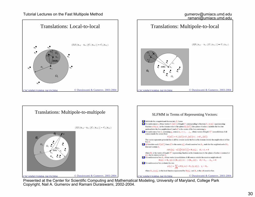
Translations: Local-to-local
x1
Ω1i
Ω2i
x*1
x*2
R (R|R)
y R
Ω1
Ω2
x*1
x*2
(R|R)
y
a1
a2
x7
x3
x5
x4
x2
x6
© Duraiswami & Gumerov, 2003-2004CSCAMM FAM04: 04/19/2004
Translations: Multipole-to-local
xi
Ω1i
Ω1
Ω2i
x*1
x*2
S
(S|R)
y
R
Rc
R2
x1x1
Ω1
Ω1Ω1
Ω2
x*1
x*2
(S|R)
y
a 1
a 2
x3x3
x2x2
x6x6
x7x7
x5x5
x4x4
© Duraiswami & Gumerov, 2003-2004CSCAMM FAM04: 04/19/2004
Translations: Multipole-to-multipole
xi
Ω1i
Ω1iΩ1i
Ω2i
x*1
x*2
S
(S|S)
y
S
Ω2
R |
x1
Ω1
Ω1Ω1
Ω2
x*1
x*2
(S|S)
y
ΩΩ
a1a2
x2x2
x4x4
x3x3
x5x5
x6x6
x7x7
© Duraiswami & Gumerov, 2003-2004CSCAMM FAM04: 04/19/2004
SLFMM in Terms of Representing Vectors:
Tutorial Lectures on the Fast Multipole Method [email protected]@umiacs.umd.edu
Presented at the Center for Scientific Computing and Mathematical Modeling, University of Maryland, College ParkCopyright, Nail A. Gumerov and Ramani Duraiswami, 2002-2004.

31
© Duraiswami & Gumerov, 2003-2004CSCAMM FAM04: 04/19/2004
Matrix Representations of Translation Operators
© Duraiswami & Gumerov, 2003-2004CSCAMM FAM04: 04/19/2004
Translation Operator
yt
y+t
© Duraiswami & Gumerov, 2003-2004CSCAMM FAM04: 04/19/2004
Example of Translation Operator
y
Φ(y)Φ(y+t)
t
T(t)
© Duraiswami & Gumerov, 2003-2004CSCAMM FAM04: 04/19/2004
R|R-reexpansion
Tutorial Lectures on the Fast Multipole Method [email protected]@umiacs.umd.edu
Presented at the Center for Scientific Computing and Mathematical Modeling, University of Maryland, College ParkCopyright, Nail A. Gumerov and Ramani Duraiswami, 2002-2004.

32
© Duraiswami & Gumerov, 2003-2004CSCAMM FAM04: 04/19/2004
Example of R|R-reexpansion
© Duraiswami & Gumerov, 2003-2004CSCAMM FAM04: 04/19/2004
R|R-translation operator
© Duraiswami & Gumerov, 2003-2004CSCAMM FAM04: 04/19/2004
Why the same operator named differently?
The first letter showsthe basis for Φ(y)
The second letter shows the basis for Φ(y +t)
Needed only to show the expansion basis (for operator representation)
© Duraiswami & Gumerov, 2003-2004CSCAMM FAM04: 04/19/2004
Matrix representation of R|R-translation operator
Consider
Coefficients ofshifted function
Coefficients oforiginal function
Tutorial Lectures on the Fast Multipole Method [email protected]@umiacs.umd.edu
Presented at the Center for Scientific Computing and Mathematical Modeling, University of Maryland, College ParkCopyright, Nail A. Gumerov and Ramani Duraiswami, 2002-2004.

33
© Duraiswami & Gumerov, 2003-2004CSCAMM FAM04: 04/19/2004
Reexpansion of the same function over shifted basis
We have:
© Duraiswami & Gumerov, 2003-2004CSCAMM FAM04: 04/19/2004
R-expansion
S-expansionx*
xiRS
Example
© Duraiswami & Gumerov, 2003-2004CSCAMM FAM04: 04/19/2004
R|R-operator
© Duraiswami & Gumerov, 2003-2004CSCAMM FAM04: 04/19/2004
S|S-operator
Tutorial Lectures on the Fast Multipole Method [email protected]@umiacs.umd.edu
Presented at the Center for Scientific Computing and Mathematical Modeling, University of Maryland, College ParkCopyright, Nail A. Gumerov and Ramani Duraiswami, 2002-2004.

34
© Duraiswami & Gumerov, 2003-2004CSCAMM FAM04: 04/19/2004
S|R-operator
© Duraiswami & Gumerov, 2003-2004CSCAMM FAM04: 04/19/2004
Renormalized R-functions
ToeplitzTranslation Matrix:
© Duraiswami & Gumerov, 2003-2004CSCAMM FAM04: 04/19/2004
Renormalized S-functions
ToeplitzTranslation Matrix:
© Duraiswami & Gumerov, 2003-2004CSCAMM FAM04: 04/19/2004
Renormalized S-functions
Hankel
Translation Matrix:
Tutorial Lectures on the Fast Multipole Method [email protected]@umiacs.umd.edu
Presented at the Center for Scientific Computing and Mathematical Modeling, University of Maryland, College ParkCopyright, Nail A. Gumerov and Ramani Duraiswami, 2002-2004.

35
© Duraiswami & Gumerov, 2003-2004CSCAMM FAM04: 04/19/2004
Integral Representations and Diagonal Forms of Translation Operators
© Duraiswami & Gumerov, 2003-2004CSCAMM FAM04: 04/19/2004
With such renormalized functions all translations can be performed with
complexity O(plogp).
But we look for something faster.
Theoretical limit for translationof vector of length p is O(p).
ONLY SPARSE TRANSLATION MATRIX CAN PROVIDESUCH COMPLEXITY
© Duraiswami & Gumerov, 2003-2004CSCAMM FAM04: 04/19/2004
Representations Based on Signature Functions
We assume thatseries for SFconverge. This is always true for finite series,Cm = 0, m > p-1.
© Duraiswami & Gumerov, 2003-2004CSCAMM FAM04: 04/19/2004
Integral Representation of Regular Functions
Property ofFourier coefficients
Regular kernel
Tutorial Lectures on the Fast Multipole Method [email protected]@umiacs.umd.edu
Presented at the Center for Scientific Computing and Mathematical Modeling, University of Maryland, College ParkCopyright, Nail A. Gumerov and Ramani Duraiswami, 2002-2004.

36
© Duraiswami & Gumerov, 2003-2004CSCAMM FAM04: 04/19/2004
Integral Representation of Regular Basis Functions
© Duraiswami & Gumerov, 2003-2004CSCAMM FAM04: 04/19/2004
Integral Representation of Singular Functions
Property ofFourier coefficients
Singular kernel
© Duraiswami & Gumerov, 2003-2004CSCAMM FAM04: 04/19/2004
Integral Representation of Singular Basis Functions
© Duraiswami & Gumerov, 2003-2004CSCAMM FAM04: 04/19/2004
R|R-translation of the Signature Function
So the R|R translation of the SF means simply multiplication of the SF by the regular kernel !
Tutorial Lectures on the Fast Multipole Method [email protected]@umiacs.umd.edu
Presented at the Center for Scientific Computing and Mathematical Modeling, University of Maryland, College ParkCopyright, Nail A. Gumerov and Ramani Duraiswami, 2002-2004.

37
© Duraiswami & Gumerov, 2003-2004CSCAMM FAM04: 04/19/2004
S|S-translation of the Signature Function
So the S|S translation of the SF means multiplication of the SF by the regular kernel.
Representation of the regular basis function
© Duraiswami & Gumerov, 2003-2004CSCAMM FAM04: 04/19/2004
S|R-translation of the Signature Function
So the S|S translation of the SF means multiplication of the SF by the singular kernel.
© Duraiswami & Gumerov, 2003-2004CSCAMM FAM04: 04/19/2004
Evaluation of Function based on its Signature Function
quadrature weights quadrature nodes
function bandwidth
quadrature order
Use Gaussian Type Quadrature
© Duraiswami & Gumerov, 2003-2004CSCAMM FAM04: 04/19/2004
FMM Data Structures
Nail Gumerov & Ramani Duraiswami
UMIACS[gumerov][ramani]@umiacs.umd.edu
Tutorial Lectures on the Fast Multipole Method [email protected]@umiacs.umd.edu
Presented at the Center for Scientific Computing and Mathematical Modeling, University of Maryland, College ParkCopyright, Nail A. Gumerov and Ramani Duraiswami, 2002-2004.

38
© Duraiswami & Gumerov, 2003-2004CSCAMM FAM04: 04/19/2004
Content• Introduction• Hierarchical Space Subdivision with 2d-Trees• Hierarchical Indexing System
Parent & Children Finding• Binary Ordering• Spatial Ordering Using Bit Interleaving
Neighbor & Box Center Finding• Spatial Data Structuring
Threshold Level of Space Subdivision• Operations on Sets
© Duraiswami & Gumerov, 2003-2004CSCAMM FAM04: 04/19/2004
Reference:
N.A. Gumerov, R. Duraiswami & E.A. Borovikov
Data Structures, Optimal Choice of Parameters, and Complexity Results for Generalized Multilevel FastMultipole Methods in d Dimensions
UMIACS TR 2003-28, Also issued as Computer Science Technical Report CS-TR-# 4458. Volume 91 pages.
University of Maryland, College Park, 2003.
AVAILABLE ONLINE VIA http://www.umiacs.umd.edu/~gumerovhttp://www.umiacs.umd.edu/~ramani
© Duraiswami & Gumerov, 2003-2004CSCAMM FAM04: 04/19/2004
Introduction
© Duraiswami & Gumerov, 2003-2004CSCAMM FAM04: 04/19/2004
FMM Data Structures
Since the complexity of FMM should not exceed O(N2) (at M~N), data organization should be provided for efficient numbering, search, and operations with these data. Some naive approaches can utilize search algorithms that result in O(N2) complexity of the FMM (and so they kill the idea of the FMM).In d-dimensions O(NlogN) complexity for operations with data can be achieved.
Tutorial Lectures on the Fast Multipole Method [email protected]@umiacs.umd.edu
Presented at the Center for Scientific Computing and Mathematical Modeling, University of Maryland, College ParkCopyright, Nail A. Gumerov and Ramani Duraiswami, 2002-2004.

39
© Duraiswami & Gumerov, 2003-2004CSCAMM FAM04: 04/19/2004
FMM Data Structures (2)Approaches include:
Data preprocessing SortingBuilding lists (such as neighbor lists): requires memory, potentially can be avoided;Building and storage of trees: requires memory, potentially can be avoided;
Operations with data during the FMM algorithm execution:Operations on data sets;Search procedures.
Preferable algorithms:Avoid unnecessary memory usage; Use fast (constant and logarithmic) search procedures;Employ bitwise operations;Can be parallelized.
Tradeoff Between Memory and Speed
© Duraiswami & Gumerov, 2003-2004CSCAMM FAM04: 04/19/2004
Space Subdivision with 2d -Trees
© Duraiswami & Gumerov, 2003-2004CSCAMM FAM04: 04/19/2004
Historically:• Binary trees (1D), Quadtrees (2D), Octrees (3D);• We will consider a concept of 2d-tree.
d=1 – binary;d=2 – quadtree;d=3 – octree;d=4 – hexatree;and so on..
© Duraiswami & Gumerov, 2003-2004CSCAMM FAM04: 04/19/2004
Hierarchy in 2d-tree
Level 1
Level 0Level 2
Level 3
ParentSelf
ChildChild
Child Child
Neighbor(Sibling)
Neighbor Neighbor Neighbor
Neighbor
NeighborNeighbor(Sibling)
Neighbor(Sibling)
Level 1
Level 0Level 2
Level 3
Level 1
Level 0Level 2
Level 3
ParentSelf
ChildChild
Child Child
Neighbor(Sibling)
Neighbor Neighbor Neighbor
Neighbor
NeighborNeighbor(Sibling)
Neighbor(Sibling)
Tutorial Lectures on the Fast Multipole Method [email protected]@umiacs.umd.edu
Presented at the Center for Scientific Computing and Mathematical Modeling, University of Maryland, College ParkCopyright, Nail A. Gumerov and Ramani Duraiswami, 2002-2004.

40
© Duraiswami & Gumerov, 2003-2004CSCAMM FAM04: 04/19/2004
2d-trees
2-tree (binary) 22-tree (quad) 2d-tree
0
1
2
3
Level
Children
Parent
Neighbor(Sibling) Maybe
Neighbor
Self
Numberof Boxes
1
2d
22d
23d
2-tree (binary) 22-tree (quad) 2d-tree
0
1
2
3
Level
Children
Parent
Neighbor(Sibling) Maybe
Neighbor
Self
Numberof Boxes
1
2d
22d
23d
© Duraiswami & Gumerov, 2003-2004CSCAMM FAM04: 04/19/2004
Hierarchical Indexing
© Duraiswami & Gumerov, 2003-2004CSCAMM FAM04: 04/19/2004
Hierarchical Indexing in 2d-trees. Index at the Level.
0 01 2
1 31
3
3
3
31
1
1
0
20 0
02 2
2
1
11
1
1
111
11
11
1 1 1
0
0
0
00 0
0
0
0
0 00
0
0
0
2
0
2 2 2 2
222
2 2
222
2
2
2
3 3 3 3
3
3
3 33
3 3 3
33330 01 2
1 31
3
3
3
31
1
1
0
20 0
02 2
2
1
11
1
1
111
11
11
1 1 1
0
0
0
00 0
0
0
0
0 00
0
0
0
2
0
2 2 2 2
222
2 2
222
2
2
2
3 3 3 3
3
3
3 33
3 3 3
3333
Indexing in quad-tree
The large black box has the indexing string (2,3). So its index is 234=1110.
The small black box hasthe indexing string (3,1,2).So its index is 3124=5410.
In general: Index (Number) at level l is:
© Duraiswami & Gumerov, 2003-2004CSCAMM FAM04: 04/19/2004
Universal Index (Number)
0 01 2
1 31
3
3
3
31
1
1
0
20 0
02 2
2
1
11
1
1
111
11
11
1 1 1
0
0
0
00 0
0
0
0
0 00
0
0
0
2
0
2 2 2 2
222
2 2
222
2
2
2
3 3 3 3
3
3
3 33
3 3 3
33330 01 2
1 31
3
3
3
31
1
1
0
20 0
02 2
2
1
11
1
1
111
11
11
1 1 1
0
0
0
00 0
0
0
0
0 00
0
0
0
2
0
2 2 2 2
222
2 2
222
2
2
2
3 3 3 3
3
3
3 33
3 3 3
3333
The large black box has the indexing string (2,3). So its index is 234=1110 at level 2
The small gray box hasthe indexing string (0,2,3).So its index is 234=1110 at level 3.
In general: Universal index is a pair:
This index at this level
Tutorial Lectures on the Fast Multipole Method [email protected]@umiacs.umd.edu
Presented at the Center for Scientific Computing and Mathematical Modeling, University of Maryland, College ParkCopyright, Nail A. Gumerov and Ramani Duraiswami, 2002-2004.

41
© Duraiswami & Gumerov, 2003-2004CSCAMM FAM04: 04/19/2004
Parent Index
0 01 2
1 31
3
3
3
31
1
1
0
20 0
02 2
2
1
11
1
1
111
11
11
1 1 1
0
0
0
00 0
0
0
0
0 00
0
0
0
2
0
2 2 2 2
222
2 2
222
2
2
2
3 3 3 3
3
3
3 33
3 3 3
33330 01 2
1 31
3
3
3
31
1
1
0
20 0
02 2
2
1
11
1
1
111
11
11
1 1 1
0
0
0
00 0
0
0
0
0 00
0
0
0
2
0
2 2 2 2
222
2 2
222
2
2
2
3 3 3 3
3
3
3 33
3 3 3
3333
Parent’s indexing string:
Parent’s index:
Parent’s universal index:
Parent index does not depend onthe level of the box! E.g. in the quad-treeat any level
Algorithm to find the parent number:
For box #234 (gray or black) the parent box index is 24. © Duraiswami & Gumerov, 2003-2004CSCAMM FAM04: 04/19/2004
Children IndexesChildren indexing strings:
Children indexes:
Children universal indexes:
Children indexes do not depend onthe level of the box! E.g. in the quad-treeat any level:
Algorithm to find the children numbers:
© Duraiswami & Gumerov, 2003-2004CSCAMM FAM04: 04/19/2004
A couple of examples:
© Duraiswami & Gumerov, 2003-2004CSCAMM FAM04: 04/19/2004
Can it be even faster?
YES!USE BITSHIFT PROCEDURES!
(HINT: Multiplication and division by 2d
are equivalent to d-bit shift.)
Tutorial Lectures on the Fast Multipole Method [email protected]@umiacs.umd.edu
Presented at the Center for Scientific Computing and Mathematical Modeling, University of Maryland, College ParkCopyright, Nail A. Gumerov and Ramani Duraiswami, 2002-2004.

42
© Duraiswami & Gumerov, 2003-2004CSCAMM FAM04: 04/19/2004
Matlab Program for Parent Finding
p = bitshift(n,-d);
Parent Box Index
Box Index
Space dimensionality
© Duraiswami & Gumerov, 2003-2004CSCAMM FAM04: 04/19/2004
Binary Ordering
© Duraiswami & Gumerov, 2003-2004CSCAMM FAM04: 04/19/2004 © Duraiswami & Gumerov, 2003-2004CSCAMM FAM04: 04/19/2004
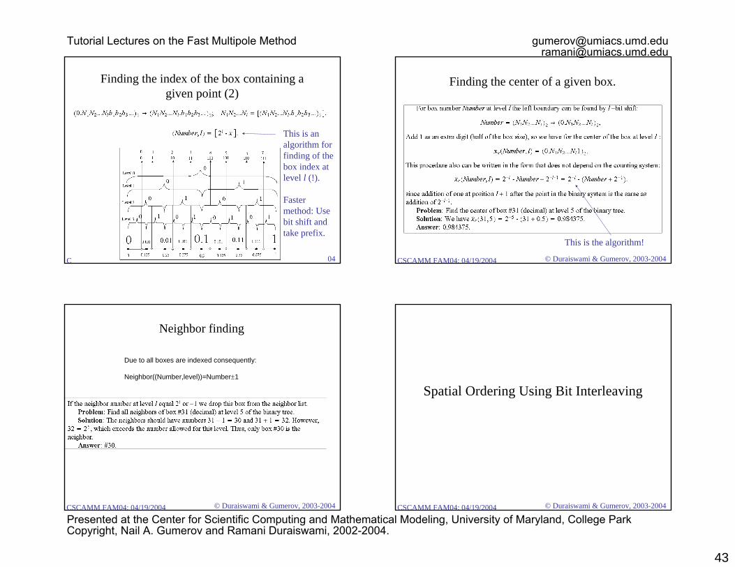
Finding the index of the box containing a given point
Level 1:
Level 2:
Level l:We use indexingstrings !
Tutorial Lectures on the Fast Multipole Method [email protected]@umiacs.umd.edu
Presented at the Center for Scientific Computing and Mathematical Modeling, University of Maryland, College ParkCopyright, Nail A. Gumerov and Ramani Duraiswami, 2002-2004.
43
© Duraiswami & Gumerov, 2003-2004CSCAMM FAM04: 04/19/2004
Finding the index of the box containing a given point (2)
This is an algorithm for finding of the box index at level l (!).
Faster method: Use bit shift and take prefix.
© Duraiswami & Gumerov, 2003-2004CSCAMM FAM04: 04/19/2004
Finding the center of a given box.
This is the algorithm!
© Duraiswami & Gumerov, 2003-2004CSCAMM FAM04: 04/19/2004
Neighbor finding
Due to all boxes are indexed consequently:
Neighbor((Number,level))=Number±1
© Duraiswami & Gumerov, 2003-2004CSCAMM FAM04: 04/19/2004
Spatial Ordering Using Bit Interleaving
Tutorial Lectures on the Fast Multipole Method [email protected]@umiacs.umd.edu
Presented at the Center for Scientific Computing and Mathematical Modeling, University of Maryland, College ParkCopyright, Nail A. Gumerov and Ramani Duraiswami, 2002-2004.

44
© Duraiswami & Gumerov, 2003-2004CSCAMM FAM04: 04/19/2004
Bit Interleaving
This maps Rd R, where coordinates are ordered naturally!
© Duraiswami & Gumerov, 2003-2004CSCAMM FAM04: 04/19/2004
Example of Bit Interleaving.
Consider 3-dimensional space, and an octree.
© Duraiswami & Gumerov, 2003-2004CSCAMM FAM04: 04/19/2004
Convention for Children Ordering.
x1
x2(0,0)
0
(0,1)1
(1,0)2
(1,1)3
x1
x3 x2
(0,0,0)
(1,0,0)
0
12
3
4
56
7
(0,1,0)
(0,1,1)(0,0,1)
(1,1,0)
(1,1,1)
(1,0,1)
x1
x2(0,0)
0
(0,1)1
(1,0)2
(1,1)3
x1
x3 x2
(0,0,0)
(1,0,0)
0
12
3
4
56
7
(0,1,0)
(0,1,1)(0,0,1)
(1,1,0)
(1,1,1)
(1,0,1)
d = 2 d = 3© Duraiswami & Gumerov, 2003-2004CSCAMM FAM04: 04/19/2004
Finding the index of the box containing a given point.
Tutorial Lectures on the Fast Multipole Method [email protected]@umiacs.umd.edu
Presented at the Center for Scientific Computing and Mathematical Modeling, University of Maryland, College ParkCopyright, Nail A. Gumerov and Ramani Duraiswami, 2002-2004.

45
© Duraiswami & Gumerov, 2003-2004CSCAMM FAM04: 04/19/2004
Finding the index of the box containing a given point. Algorithm and Example.
© Duraiswami & Gumerov, 2003-2004CSCAMM FAM04: 04/19/2004
Bit Deinterleaving
© Duraiswami & Gumerov, 2003-2004CSCAMM FAM04: 04/19/2004
Bit deinterleving (2). Example.
100101100010111012
Number3 = 0 0 0 1 1 1 = 1112 = 710Number2 = 1 1 1 0 1 0 = 1110102 = 5810Number1 = 0 1 0 0 1 = 10012 = 910
Number = 7689310
100101100010111012
Number3 = 0 0 0 1 1 1 = 1112 = 710Number2 = 1 1 1 0 1 0 = 1110102 = 5810Number1 = 0 1 0 0 1 = 10012 = 910
Number = 7689310 To break the number into groupsof d bits start fromthe last digit!
It is OK that the first group is incomplete
© Duraiswami & Gumerov, 2003-2004CSCAMM FAM04: 04/19/2004
Finding the center of a given box.
Tutorial Lectures on the Fast Multipole Method [email protected]@umiacs.umd.edu
Presented at the Center for Scientific Computing and Mathematical Modeling, University of Maryland, College ParkCopyright, Nail A. Gumerov and Ramani Duraiswami, 2002-2004.
46
© Duraiswami & Gumerov, 2003-2004CSCAMM FAM04: 04/19/2004
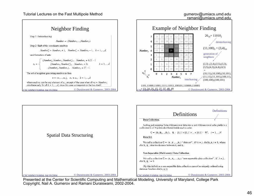
Neighbor Finding
© Duraiswami & Gumerov, 2003-2004CSCAMM FAM04: 04/19/2004
Example of Neighbor Finding
17
5
2921
1
45
574925
6153
3713
9 33 41
20
4
16
80 32
28
40
24
12 4436
56
52
48
2
60
6 14 38 46
423410
26 50
625430
18
22
58
23 31 55 63
19
7
27 5951
15 39 47
4335113
x1
x2 0 1 2 3 4 5 6 7Number1
0
1
2
3
4
5
6
7
Number2
17
5
2921
1
45
574925
6153
3713
9 33 41
20
4
16
80 32
28
40
24
12 4436
56
52
48
2
60
6 14 38 46
423410
26 50
625430
18
22
58
23 31 55 63
19
7
27 5951
15 39 47
4335113
x1
x2 0 1 2 3 4 5 6 7Number1
0
1
2
3
4
5
6
7
Number2
2610= 110102
(11,100)2 = (3,4)10
deinterleaving
generation of neighbors
(2,3) ,(2,4),(2,5),(3,3),(3,5),(4,3),(4,4),(4,5)=
(10,11),(10,100),(10,101),(11,11),(11,101),(100,11),(100,100),(100,101)interleaving
1101,11000,11001,1111,11011,100101,110000,110001= 13, 24, 25, 15, 27, 37, 48, 49
© Duraiswami & Gumerov, 2003-2004CSCAMM FAM04: 04/19/2004
Spatial Data Structuring
© Duraiswami & Gumerov, 2003-2004CSCAMM FAM04: 04/19/2004
DefinitionsDefinitions
Tutorial Lectures on the Fast Multipole Method [email protected]@umiacs.umd.edu
Presented at the Center for Scientific Computing and Mathematical Modeling, University of Maryland, College ParkCopyright, Nail A. Gumerov and Ramani Duraiswami, 2002-2004.

47
© Duraiswami & Gumerov, 2003-2004CSCAMM FAM04: 04/19/2004
Threshold Level
© Duraiswami & Gumerov, 2003-2004CSCAMM FAM04: 04/19/2004
Spatial Data Sorting
© Duraiswami & Gumerov, 2003-2004CSCAMM FAM04: 04/19/2004
Spatial Data Sorting (2)
• Before sorting represent your data with maximum number of bits available (or intended to use). This corresponds to maximum level Lavailable available (say [Lavailable=BitMax/d].
• In the hierarchical 2d-tree space subdivision the sorted list will remain sorted at any level L< Lavailable. So the data ordering is required only one time.
© Duraiswami & Gumerov, 2003-2004CSCAMM FAM04: 04/19/2004
After data sorting we need tofind the maximum level of space subdivision that will be
employed
In Multilevel FMM two following conditions can be mainly considered:
• At level Lmax each box contains not more than s points (s is called clustering or grouping parameter)• At level Lmax the neighborhood of each box contains not more than q points.
Tutorial Lectures on the Fast Multipole Method [email protected]@umiacs.umd.edu
Presented at the Center for Scientific Computing and Mathematical Modeling, University of Maryland, College ParkCopyright, Nail A. Gumerov and Ramani Duraiswami, 2002-2004.

48
© Duraiswami & Gumerov, 2003-2004CSCAMM FAM04: 04/19/2004
The threshold level determination algorithm in O(N) time
s is the clustering parameter
© Duraiswami & Gumerov, 2003-2004CSCAMM FAM04: 04/19/2004
Binary Search in Sorted List
• Operation of getting non-empty boxes at any level L(say neighbors) can be performed with O(logN) complexity for any fixed d.
• It consists of obtaining a small list of all neighbor boxes with O(1) complexity and• Binary search of each neighbor in the sorted list at level L is an O(Ld) operation.• For small L and d this is almost O(1) procedure.
© Duraiswami & Gumerov, 2003-2004CSCAMM FAM04: 04/19/2004
Operations on Sets
© Duraiswami & Gumerov, 2003-2004CSCAMM FAM04: 04/19/2004
Tutorial Lectures on the Fast Multipole Method [email protected]@umiacs.umd.edu
Presented at the Center for Scientific Computing and Mathematical Modeling, University of Maryland, College ParkCopyright, Nail A. Gumerov and Ramani Duraiswami, 2002-2004.

49
© Duraiswami & Gumerov, 2003-2004CSCAMM FAM04: 04/19/2004
The Multilevel Fast Multipole Method
Ramani DuraiswamiNail Gumerov
© Duraiswami & Gumerov, 2003-2004CSCAMM FAM04: 04/19/2004
Review• FMM aims at accelerating
the matrix vector product• Matrix entries determined by
a set of source points and evaluation points (possiblythe same)
• Function Φ has following point-centered representations about a given point x*
Local (valid in a neighborhood of a given point)Far-field or multipole (valid outside a neighborhood of a given point)In many applications Φ is singular
• Representations are usually series Could be integral transform representations
• Representations are usually approximate Error bound guarantees the error is below a specified tolerance
© Duraiswami & Gumerov, 2003-2004CSCAMM FAM04: 04/19/2004
Review• One representation, valid in a
given domain, can be converted to another valid in a subdomaincontained in the original domain
• Factorization trick is at core of the FMM speed up
• Representations we use are factored … separate points xi and yj
• Data is partitioned to organize the source points and evaluation points so that for each point we can separate the points over which we can use the factorization trick, and those we cannot.
• Hierarchical partitioning allows use of different factorizations for different groups of points
• Accomplished via MLFMM
© Duraiswami & Gumerov, 2003-2004CSCAMM FAM04: 04/19/2004
Prepare Data Structures
• Convert data set into integers given some maximum number of bits allowed/dimensionality of space
• Interleave• Sort• Go through the list and check at what bit position two
strings differ For a given s determine the number of levels of subdivision neededs is the maximum number of points in a box at the finest level
Tutorial Lectures on the Fast Multipole Method [email protected]@umiacs.umd.edu
Presented at the Center for Scientific Computing and Mathematical Modeling, University of Maryland, College ParkCopyright, Nail A. Gumerov and Ramani Duraiswami, 2002-2004.

50
© Duraiswami & Gumerov, 2003-2004CSCAMM FAM04: 04/19/2004
Hierarchical Spatial Domains
Ε1
Ε3Ε4
Ε2Ε1
Ε3Ε4
Ε2E1: box
E2: points in the box and in neighboring boxes
E3: points in boxes outside neighborhood
E4: points belonging to neighbors of parent box, but which do not belong to E2
© Duraiswami & Gumerov, 2003-2004CSCAMM FAM04: 04/19/2004
|y - x* - t| > r 1 = r + |t|
Since Ωr1(x*+t) ⊂ Ωr(t) !
xi
Ω1
Ω2x*1
x*2
S
(S|S)
S
xi
x*
x*+t(S|S)
y
t
Ωr1(x*+t)Ωr(x*)
rr1
Original expansionIs valid only here!
Also|xi - x* | < r
singular point !
S|S-reexpansion (Far to Far, or Multipole to Multipole, or M2M)
© Duraiswami & Gumerov, 2003-2004CSCAMM FAM04: 04/19/2004
UPWARD PASS• Partition sources into a source hierarchy.• Stop hierarchy so that boxes at the finest level contain at most s
sources• Let the number of levels be L• Consider the finest level• For non-empty boxes we create S expansion about center of the
box Φ(xi,y)=∑P uiB(x*,xi) S(x*,y)
• We need to keep these coefficients. C(n,l) for each level as we will need it in the downward pass
• Then use S/S translations to go up level by level up to level 2.• Cannot go to level 1 (Why?)
© Duraiswami & Gumerov, 2003-2004CSCAMM FAM04: 04/19/2004
• S expansion is valid in the domain E_3 outside domain E_1 (provided d<9)
Ε1
Ε1
ΕΕ3
xi
xc(n,L)
y
Tutorial Lectures on the Fast Multipole Method [email protected]@umiacs.umd.edu
Presented at the Center for Scientific Computing and Mathematical Modeling, University of Maryland, College ParkCopyright, Nail A. Gumerov and Ramani Duraiswami, 2002-2004.

51
© Duraiswami & Gumerov, 2003-2004CSCAMM FAM04: 04/19/2004
UPWARD PASS• At the end of the upward pass we have a set of S
expansions (i.e. we have coefficients for them)• we have a set of coefficients C(n,l) for n=1,…,2ld l=L,…,2 • Each of these expansions is about a center, and is valid
in some domain• We would like to use the coarsest expansions in the
downward pass (have to deal with fewest numbers of coefficients)
• But may not be able to --- because of domain of validity• Upward pass works on source points and builds
representations to be used in the downward pass, where the actual product will be evaluated
© Duraiswami & Gumerov, 2003-2004CSCAMM FAM04: 04/19/2004
DOWNWARD PASS• Starting from level 2, build an R expansion in boxes
where R expansion is valid
• Must to do S|R translation • The S expansion is not valid in
boxes immediately surrounding the current box
• So we must exclude boxes in the E4 neighborhood
Ε 4Ε 4
© Duraiswami & Gumerov, 2003-2004CSCAMM FAM04: 04/19/2004
Ωr(x*)|y - x* - t| < r 1 = |t| - r
Since Ωr1(x*+t) ⊂ Ωr(t) !
Original expansionIs valid only here!
Also|xi - x* | < r
singular point !
xi
Ω1
x*1
x*2
S
(S|S)
S
xi
x*
x*+t
(S|R)
y
t
Ωr1(x*+t)
r
r1
S|R-reexpansion (Far to Local, or Multipole to Local, or M2L)
© Duraiswami & Gumerov, 2003-2004CSCAMM FAM04: 04/19/2004
Downward Pass. Step 1.Level 2: Level 3:
Tutorial Lectures on the Fast Multipole Method [email protected]@umiacs.umd.edu
Presented at the Center for Scientific Computing and Mathematical Modeling, University of Maryland, College ParkCopyright, Nail A. Gumerov and Ramani Duraiswami, 2002-2004.

52
© Duraiswami & Gumerov, 2003-2004CSCAMM FAM04: 04/19/2004
Downward Pass. Step 1.
THIS MIGHT BETHE MOST EXPENSIVESTEP OF THE ALGORITHM
© Duraiswami & Gumerov, 2003-2004CSCAMM FAM04: 04/19/2004
Downward Pass. Step 1.
Total number of S|R-translationsper 1 box in d-dimensional space
(far from the domain boundaries)
ExponentialGrowth
© Duraiswami & Gumerov, 2003-2004CSCAMM FAM04: 04/19/2004
Domains of Expansion Validity (6).S|R-translation.
x*1 x*2yxi d < 4
< <
< <
© Duraiswami & Gumerov, 2003-2004CSCAMM FAM04: 04/19/2004
R|R-reexpansion (Local to Local, or L2L)
|y - x* - t| < r 1 = r - |t|
Since Ωr1(x*+t) ⊂ Ωr(t) !
Original expansionIs valid only here!
Ω1
Ω2
x*1
x*2
R (R|R)
xR
Ωr(x*)
x*
(R|R)
y x*+tt
r
Ωr1(x*+t)
r1
Tutorial Lectures on the Fast Multipole Method [email protected]@umiacs.umd.edu
Presented at the Center for Scientific Computing and Mathematical Modeling, University of Maryland, College ParkCopyright, Nail A. Gumerov and Ramani Duraiswami, 2002-2004.

53
© Duraiswami & Gumerov, 2003-2004CSCAMM FAM04: 04/19/2004
Downward Pass Step 2• Now consider we already have done the S|R translation at
some level at the center of a box.• So we have a R expansion that includes contribution of
most of the points, but not of points in the E4 neighborhood• We can go to a finer level to include these missed points• But we will now have to translate the already built R
expansion to a box center of a child(Makes no sense to do S|R again, since many S|R are consolidated in this R expansion)
• Add to this translated one, the S|R of the E4 of the finer level
© Duraiswami & Gumerov, 2003-2004CSCAMM FAM04: 04/19/2004
• Formally
© Duraiswami & Gumerov, 2003-2004CSCAMM FAM04: 04/19/2004
Downward Pass. Step 2.
© Duraiswami & Gumerov, 2003-2004CSCAMM FAM04: 04/19/2004
Domains of Expansion Validity (5).R|R and S|S-translations.
S|S R|R
x*1
x*2
y
xi
y
xi
x*1
x*2
Not as restrictive as S|R
Tutorial Lectures on the Fast Multipole Method [email protected]@umiacs.umd.edu
Presented at the Center for Scientific Computing and Mathematical Modeling, University of Maryland, College ParkCopyright, Nail A. Gumerov and Ramani Duraiswami, 2002-2004.

54
© Duraiswami & Gumerov, 2003-2004CSCAMM FAM04: 04/19/2004
Final Summation
• At this point we are at the finest level. • We cannot do any S|R translation for xi ‘s that are in the
E_3 neighborhood of our yj’s• Must evaluate these directly
© Duraiswami & Gumerov, 2003-2004CSCAMM FAM04: 04/19/2004
Final Summation
yj
Contribution of E2 Contribution of E3
© Duraiswami & Gumerov, 2003-2004CSCAMM FAM04: 04/19/2004
Cost of FMM --- Upward Pass
• Upward Step1. Cost of creating an S expansion for each source point. O(NP)
• Upward Step2. Cost of performing an S|S translation If we use expensive (matrix vector) method cost is O(P2) for one translation.
• Step 2 is repeated from level L-1 to level 2
• Total Cost of Upward Pass ∼ NP + (N/s) (P2)
© Duraiswami & Gumerov, 2003-2004CSCAMM FAM04: 04/19/2004
COST of MLFMM• Cost of downward pass, step 1 is the cost of performing
S|R translations at each level
• At the downward pass, 2nd step we have the cost of the R|R translation, and S|R translation from the E4neighbourhood (already accounted for above)
• Final summation cost is
• Total
Tutorial Lectures on the Fast Multipole Method [email protected]@umiacs.umd.edu
Presented at the Center for Scientific Computing and Mathematical Modeling, University of Maryland, College ParkCopyright, Nail A. Gumerov and Ramani Duraiswami, 2002-2004.

55
© Duraiswami & Gumerov, 2003-2004CSCAMM FAM04: 04/19/2004
Itemized Cost of MLFMMAssume that all translation costs are the same,CostTranslation(P)
Powers of E4and E2 neighborhoods
Regular mesh:
© Duraiswami & Gumerov, 2003-2004CSCAMM FAM04: 04/19/2004
Optimization of the Grouping Parameter
s
CostMLFMM
sopt
© Duraiswami & Gumerov, 2003-2004CSCAMM FAM04: 04/19/2004
Optimization of the Grouping Parameter(Example)
In this example optimization results in about 10 times savings!© Duraiswami & Gumerov, 2003-2004CSCAMM FAM04: 04/19/2004
DEMO• Yang Wang ([email protected]),
“Java Implementation and Simulation of the Fast Multipole Method for 2-D Coulombic Potential Problems,” AMSC 698R course project report, 2003.
• http://brigade.umiacs.umd.edu/~wpwy/applet/FmmApplet.html• Seems to work with Mozilla and Netscape …IE has problems
Tutorial Lectures on the Fast Multipole Method [email protected]@umiacs.umd.edu
Presented at the Center for Scientific Computing and Mathematical Modeling, University of Maryland, College ParkCopyright, Nail A. Gumerov and Ramani Duraiswami, 2002-2004.

56
© Duraiswami & Gumerov, 2003-2004CSCAMM FAM04: 04/19/2004
Some Numerical Experiments with MLFMM
N.A. Gumerov, R. Duraiswami & E.A. Borovikov
Data Structures, Optimal Choice of Parameters, andComplexity Results for Generalized Multilevel Fast MultipoleMethods in d Dimensions.
UMIACS TR 2003-28,Also issued as Computer Science Technical Report CS-TR-# 4458.University of Maryland, College Park, 2003.
Available online via http://www.umiacs.umd.edu/~ramani/pubs/umiacs-tr-2003-28.pdf
© Duraiswami & Gumerov, 2003-2004CSCAMM FAM04: 04/19/2004
Error Test. FMM vs Middleman.
1.E-14
1.E-13
1.E-12
1.E-11
1.E-10
1.E-09
1.E-08
1.E-07
100 1000 10000 100000
Number of Points
Abso
lute
Max
imum
Erro
r .
FMM
MediatorMiddleman
Regular Mesh, N = M.
© Duraiswami & Gumerov, 2003-2004CSCAMM FAM04: 04/19/2004
Test with Varying Grouping Parameter.
0.1
1
10
100
1 10 100 1000Number of Points in the Smallest Box
CP
U T
ime
(s)
N=1024
4096
16384
65536
Regular Mesh, d=2
5
4
5
5
5
3
4
4
3
3
2
2
1
6
7 6
6
Max Level=8
7
© Duraiswami & Gumerov, 2003-2004CSCAMM FAM04: 04/19/2004
Test with Varying N.
0.01
0.1
1
10
100
1000
1000 10000 100000 1000000Number of Points
CP
U T
ime
(s)
Straightforward
FMM (s=4)FMM/(a*log(N))
Setting FMM
Mediator
y=bx
y=cx2
Regular Mesh, d=2
Middleman
Tutorial Lectures on the Fast Multipole Method [email protected]@umiacs.umd.edu
Presented at the Center for Scientific Computing and Mathematical Modeling, University of Maryland, College ParkCopyright, Nail A. Gumerov and Ramani Duraiswami, 2002-2004.

57
© Duraiswami & Gumerov, 2003-2004CSCAMM FAM04: 04/19/2004
Comparisons for different dimensionalities
0.01
0.1
1
10
100
1000
1000 10000 100000Number of Points
CP
U T
ime
(s)
- d=1, s=8…15- d=2, s=4…15- d=3, s=8…63- d=4, s=16…256
d=1
2
3
4
Regular mesh, optimal s
y=ax
© Duraiswami & Gumerov, 2003-2004CSCAMM FAM04: 04/19/2004
Random Distributions
© Duraiswami & Gumerov, 2003-2004CSCAMM FAM04: 04/19/2004
Dependence of CPU Time on the Grouping Parameter, s
0.1
1
10
1 10 100 1000Number of Points in the Smallest Box
CP
U T
ime
(s)
MaxLevel=5
6
4
3
13
9
6
778 4
N=4096, d=2
Regular Mesh
Uniform RandomDistribution
© Duraiswami & Gumerov, 2003-2004CSCAMM FAM04: 04/19/2004
Dependence of CPU Time on the Maximum Space Subdivision Level
0.1
1
10
100
0 5 10 15Maximum Level
CP
U T
ime
(s)
N=1024
4096
16384
65536
Uniform RandomDistribution
RegularMesh
d=2
Tutorial Lectures on the Fast Multipole Method [email protected]@umiacs.umd.edu
Presented at the Center for Scientific Computing and Mathematical Modeling, University of Maryland, College ParkCopyright, Nail A. Gumerov and Ramani Duraiswami, 2002-2004.

58
© Duraiswami & Gumerov, 2003-2004CSCAMM FAM04: 04/19/2004
Dependence of CPU Time on M
0.1
1
10
100
1000 10000 100000 1000000Number of Evaluation Points
CP
U T
ime
(s)
Max Level=6
Optimum Max Level
Uniform Random DistributionsN=4096, d=2
© Duraiswami & Gumerov, 2003-2004CSCAMM FAM04: 04/19/2004
Adaptive FMM• H. Cheng, L. Greengard, and V. Rokhlin, “A Fast
Adaptive Multipole Algorithms in Three Dimensions,” Journal of Computational Physics, 155:468-498, 1999 .
• N.A. Gumerov, R. Duraiswami, and Y.A. Borovikov, “Data structures and algorithms for adaptive multilevel fast multipole methods,” in preparation.
© Duraiswami & Gumerov, 2003-2004CSCAMM FAM04: 04/19/2004
Fast Multipole Methods for The Laplace Equation
Ramani DuraiswamiNail Gumerov
© Duraiswami & Gumerov, 2003-2004CSCAMM FAM04: 04/19/2004
Outline• 3D Laplace equation and Coulomb potentials• Multipole and local expansions• Special functions
Legendre polynomialsAssociated Legendre functionsSpherical harmonics
• Translations of elementary solutions• Complexity of FMM• Reducing complexity• Rotations of elementary solutions• Coaxial Translation-Rotation decomposition• Faster Translation techniques
Tutorial Lectures on the Fast Multipole Method [email protected]@umiacs.umd.edu
Presented at the Center for Scientific Computing and Mathematical Modeling, University of Maryland, College ParkCopyright, Nail A. Gumerov and Ramani Duraiswami, 2002-2004.

59
© Duraiswami & Gumerov, 2003-2004CSCAMM FAM04: 04/19/2004
Review• FMM aims at accelerating
the matrix vector product• Matrix entries determined by
a set of source points and evaluation points (possiblythe same)
• Function Φ has following point-centered representations about a given point x*
Local (valid in a neighborhood of a given point)Far-field or multipole (valid outside a neighborhood of a given point)In many applications Φ is singular
• Representations are usually series Could be integral transform representations
• Representations are usually approximate Error bound guarantees the error is below a specified tolerance
© Duraiswami & Gumerov, 2003-2004CSCAMM FAM04: 04/19/2004
Review• One representation, valid in a
given domain, can be converted to another valid in a subdomaincontained in the original domain
• Factorization trick is at core of the FMM speed up
• Representations we use are factored … separate points xi and yj
• Data is partitioned to organize the source points and evaluation points so that for each point we can separate the points over which we can use the factorization trick, and those we cannot.
• Hierarchical partitioning allows use of different factorizations for different groups of points
• Accomplished via MLFMM discussed yesterday• Today concrete example for Laplace equation/Coulomb potentials
© Duraiswami & Gumerov, 2003-2004CSCAMM FAM04: 04/19/2004
Solution of Laplace’s equation• Green’s function for Laplace’s equation
• Green’s formula
• Goal solve Laplace’s equation with given boundary conditionsE.g. ∇2 φ =0 in Ω ∂ φ/∂ n =f on ∂ Ω
• Upon discretization yields system of type that can be solved iteratively, with matrix vector products accelerated by FMM
∇2G(x,y) = δ(x− y) G(x,y) = − 1
4πx− y
φ(y) =ZΩφ(x)δ(x− y)d3x =
ZΩφ(x)∇2G(x, y)d3x
= −ZΩ∇φ(x) ·∇G(x,y)d3x+
Z∂Ω
φ(x)n ·∇G(x,y)dSx=
ZΩ∇2φ(x)∇G(x,y)d3x+
Z∂Ω[φ(x)n ·∇G(x, y) − n ·∇φ(x)G(x,y)] dSx
φ(y)−Z∂Ω
φ(x)∂G
∂n(x,y) = −
Z∂Ωf(x)G(x,y)dSx
© Duraiswami & Gumerov, 2003-2004CSCAMM FAM04: 04/19/2004
Molecular and stellar dynamics• Many particles distributed in space• Particles are moving and exert a
force on each other• Simplest case this force obeys an
inverse-square law (gravity, coulombic interaction)
• Goal of computationscompute the dynamics
• Force is
• After time step, particles move
• Recompute force and iterate
2
2 ,ii
d Fdt
=x
31
( )| |
Ni j
i i jj i jj i
F q q=≠
−=
−∑x xx x
Tutorial Lectures on the Fast Multipole Method [email protected]@umiacs.umd.edu
Presented at the Center for Scientific Computing and Mathematical Modeling, University of Maryland, College ParkCopyright, Nail A. Gumerov and Ramani Duraiswami, 2002-2004.

60
© Duraiswami & Gumerov, 2003-2004CSCAMM FAM04: 04/19/2004
What is needed for the FMM• Local expansion• Far-field or multipole expansion• Translations
Multipole-to-multipole (S|S)Local-to-local (R|R)Multipole-to-local (S|R)
• Error bounds
© Duraiswami & Gumerov, 2003-2004CSCAMM FAM04: 04/19/2004
Translation and Differentiation Properties for Laplace Equation
© Duraiswami & Gumerov, 2003-2004CSCAMM FAM04: 04/19/2004
Introduction of Multipoles for Laplace Equation
© Duraiswami & Gumerov, 2003-2004CSCAMM FAM04: 04/19/2004
Multipole Expansion of LaplaceEquation Solutions
Tutorial Lectures on the Fast Multipole Method [email protected]@umiacs.umd.edu
Presented at the Center for Scientific Computing and Mathematical Modeling, University of Maryland, College ParkCopyright, Nail A. Gumerov and Ramani Duraiswami, 2002-2004.
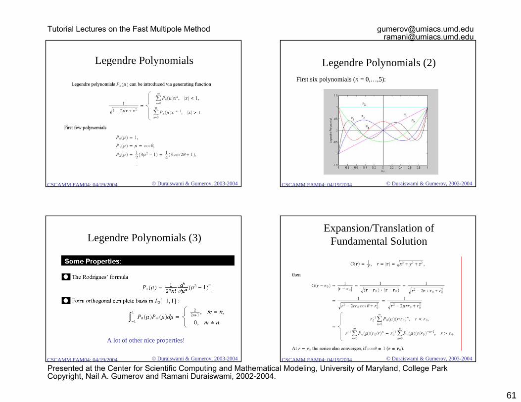
61
© Duraiswami & Gumerov, 2003-2004CSCAMM FAM04: 04/19/2004
Legendre Polynomials
© Duraiswami & Gumerov, 2003-2004CSCAMM FAM04: 04/19/2004
Legendre Polynomials (2)First six polynomials (n = 0,…,5):
© Duraiswami & Gumerov, 2003-2004CSCAMM FAM04: 04/19/2004
Legendre Polynomials (3)
A lot of other nice properties!
© Duraiswami & Gumerov, 2003-2004CSCAMM FAM04: 04/19/2004
Expansion/Translation of Fundamental Solution
Tutorial Lectures on the Fast Multipole Method [email protected]@umiacs.umd.edu
Presented at the Center for Scientific Computing and Mathematical Modeling, University of Maryland, College ParkCopyright, Nail A. Gumerov and Ramani Duraiswami, 2002-2004.
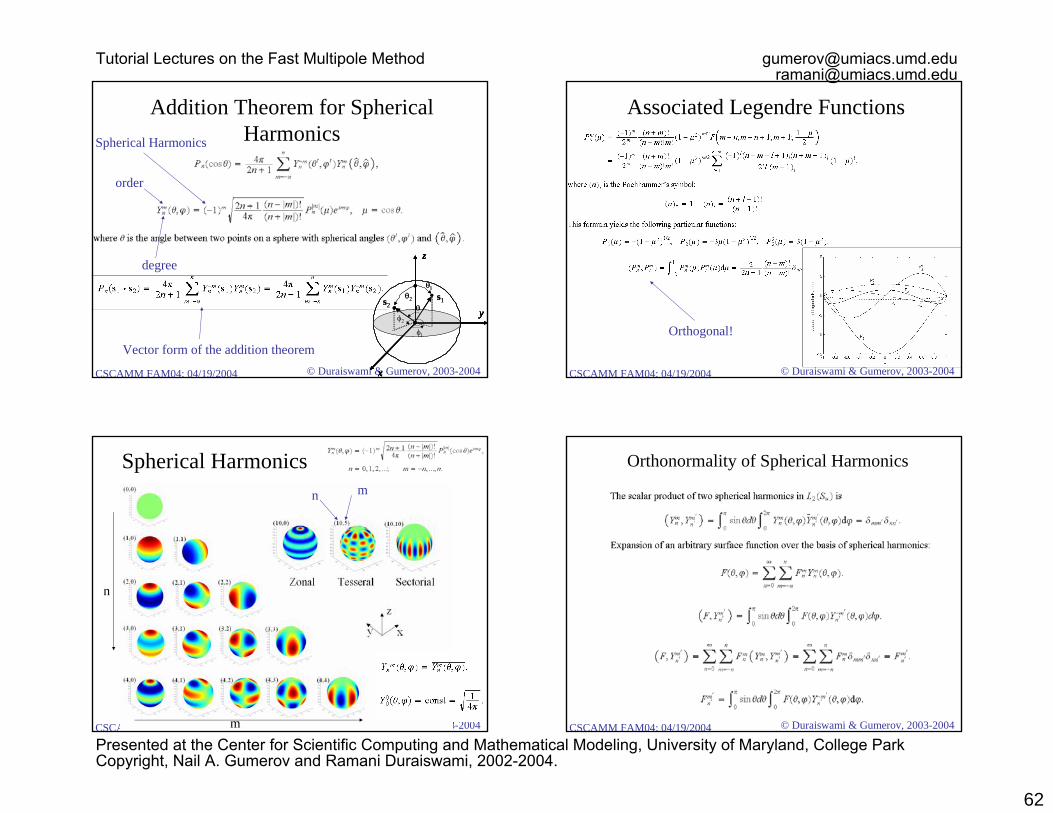
62
© Duraiswami & Gumerov, 2003-2004CSCAMM FAM04: 04/19/2004
Addition Theorem for Spherical HarmonicsSpherical Harmonics
x
y
z
x
y
z
x
y
z
θ1
φ1
s1
φ2
θ2s2 θ
x
y
z
x
y
z
x
y
z
θ1
φ1
s1
φ2
θ2s2 θ
degree
order
Vector form of the addition theorem© Duraiswami & Gumerov, 2003-2004CSCAMM FAM04: 04/19/2004
Associated Legendre Functions
Orthogonal!
© Duraiswami & Gumerov, 2003-2004CSCAMM FAM04: 04/19/2004
Spherical Harmonicsn m
n
m © Duraiswami & Gumerov, 2003-2004CSCAMM FAM04: 04/19/2004
Orthonormality of Spherical Harmonics
Tutorial Lectures on the Fast Multipole Method [email protected]@umiacs.umd.edu
Presented at the Center for Scientific Computing and Mathematical Modeling, University of Maryland, College ParkCopyright, Nail A. Gumerov and Ramani Duraiswami, 2002-2004.

63
© Duraiswami & Gumerov, 2003-2004CSCAMM FAM04: 04/19/2004
S- and R- expansions of Fundamental Solution
Multipole (!)
x
y
z
O
x
y
z
O
x
y
z
Oθ
φ
r
rir
iθ
iφ
x
y
z
O
x
y
z
O
x
y
z
Oθ
φ
r
rir
iθ
iφ
© Duraiswami & Gumerov, 2003-2004CSCAMM FAM04: 04/19/2004
Error bound
Φ(P) =kXi=1
qikPi − P k
potential due to a set of k sources of strengths qi, i = 1, . . . , k at Pi =(ri, θi,φi ), i = 1, . . . , k, with |ri| < a. Then for P = (r,θ, φ) ∈ R3 with |r| > a,
Φ(P ) =∞Xn=0
nXm=−n
Mmn
rn+1Y mn (θ,φ),
Mmn =
kXi=1
(−1)mqi ∗ rni ∗ Y −mn (θi, φi) .¯¯Φ(P )−
pXn=0
nXm=−n
Mmn
rn+1Y mn (θ, φ)
¯¯ ≤ A
r − a (a
r)p+1 ,
A =kXi=1
|qi |.
• Series converge rapidly E.g,. For multipole expansion we have
© Duraiswami & Gumerov, 2003-2004CSCAMM FAM04: 04/19/2004
`Multipole expansion` is S-expansion
© Duraiswami & Gumerov, 2003-2004CSCAMM FAM04: 04/19/2004
R- and S- expansions of arbitrary solutions of the 3D Laplace equation
Tutorial Lectures on the Fast Multipole Method [email protected]@umiacs.umd.edu
Presented at the Center for Scientific Computing and Mathematical Modeling, University of Maryland, College ParkCopyright, Nail A. Gumerov and Ramani Duraiswami, 2002-2004.

64
© Duraiswami & Gumerov, 2003-2004CSCAMM FAM04: 04/19/2004
Translations of elementary solutions of the 3D Laplace equation
For a p-truncated expansion (E|F) is a p2× p2 matrix
See Tang 03 or Greengard 89 for explicit expressions
© Duraiswami & Gumerov, 2003-2004CSCAMM FAM04: 04/19/2004
Translation of a Multipole Expansion
© Duraiswami & Gumerov, 2003-2004CSCAMM FAM04: 04/19/2004
Translation of a Local Expansion
© Duraiswami & Gumerov, 2003-2004CSCAMM FAM04: 04/19/2004
Complexity Analysis
Tutorial Lectures on the Fast Multipole Method [email protected]@umiacs.umd.edu
Presented at the Center for Scientific Computing and Mathematical Modeling, University of Maryland, College ParkCopyright, Nail A. Gumerov and Ramani Duraiswami, 2002-2004.

65
© Duraiswami & Gumerov, 2003-2004CSCAMM FAM04: 04/19/2004
Rotations of coordinates
x
y
z
x
y
z
O
AAβ
α
x
yz
x
y
z
OA
Aβ
x
y
z
x
y
z
O
AA
x
y
z
xx
yy
zz
O
AAA
x
yz
x
y
z
OA
A
x
yz
xx
yy
zz
OA
AA
γ
x
y
z
x
y
z
O
AAβ
α
x
yz
x
y
z
OA
Aβ
x
y
z
x
y
z
O
AA
x
y
z
xx
yy
zz
O
AAA
x
yz
x
y
z
OA
A
x
yz
xx
yy
zz
OA
AA
γ
iz
iy
ix
iyαE
iz
^ix
^iy
βE
γE~
iz
iy
ix
iyαE
iz
^ix
^iy
βE
γE
iz
iy
ix
iyαE
iziz
^ixix
^iyiy
βE
γE~
Rotation Matrix
Euler Angles
Spherical Polar Angles
© Duraiswami & Gumerov, 2003-2004CSCAMM FAM04: 04/19/2004
Rotations of elementary solutions of the 3D Laplace equation
© Duraiswami & Gumerov, 2003-2004CSCAMM FAM04: 04/19/2004
Rotation-Coaxial Translation Decomposition
z
yy
xx
yx
z
yx
z
zp4
p3 p3
p3
Coaxial Translation
Rotation
x
y
z
x
y
z
O
AAβ
α
x
yz
x
y
z
OA
Aβ
x
y
z
x
y
z
O
AA
x
y
z
xx
yy
zz
O
AAA
x
yz
x
y
z
OA
A
x
yz
xx
yy
zz
OA
AA
γ
x
y
z
x
y
z
O
AAβ
α
x
yz
x
y
z
OA
Aβ
x
y
z
x
y
z
O
AA
x
y
z
xx
yy
zz
O
AAA
x
yz
x
y
z
OA
A
x
yz
xx
yy
zz
OA
AA
γ
© Duraiswami & Gumerov, 2003-2004CSCAMM FAM04: 04/19/2004
Coaxial translation operator has invariant subspaces at fixed order, m,
while the rotation operator has invariant subspaces at fixed degree, n.
Each can be done in p operations which cost O(p2) resulting in O(p3) complexity
Tutorial Lectures on the Fast Multipole Method [email protected]@umiacs.umd.edu
Presented at the Center for Scientific Computing and Mathematical Modeling, University of Maryland, College ParkCopyright, Nail A. Gumerov and Ramani Duraiswami, 2002-2004.

66
© Duraiswami & Gumerov, 2003-2004CSCAMM FAM04: 04/19/2004
Comparison of Direct Matrix Translation and Coaxial Translation-Rotation Decomposition
0.01
0.1
1
10
10 100
Truncation Number, p
CP
U T
ime
(s)
Full Matrix Translation
Rotational-Coaxial Translation Decomposition
y=ax4
y=bx3
kt=86
© Duraiswami & Gumerov, 2003-2004CSCAMM FAM04: 04/19/2004
Renormalized S- and R- functions
Other Fast translation schemes: Elliot and Board (1996)
© Duraiswami & Gumerov, 2003-2004CSCAMM FAM04: 04/19/2004
Other Fast translation schemes: Elliot and Board (1996)
In the renormalized basis translation matrices are simple
These are structured matrices (2D Toeplitz-Hankel type)Fast translation procedures are possible(e.g. see O(p2logp) algorithm in W.D. Elliott & J.A. Board, Jr.:``Fast Fourier Transform Accelerated Fast Multipole Algorithm”SIAM J. Sci. Comput. Vol. 17, No. 2, pp. 398-415, 1996).However, there are some stability issues reported.
© Duraiswami & Gumerov, 2003-2004CSCAMM FAM04: 04/19/2004
Structured matrix based translation• Tang 03• Idea: use the rotation-coaxial translation method, and
decompose resulting matrices into structured matrices• Cost O(p2 log p)• Details in Tang’s thesis.http://www.umiacs.umd.edu/~ramani/pubs/zhihui_thesis.pdf
Tutorial Lectures on the Fast Multipole Method [email protected]@umiacs.umd.edu
Presented at the Center for Scientific Computing and Mathematical Modeling, University of Maryland, College ParkCopyright, Nail A. Gumerov and Ramani Duraiswami, 2002-2004.

67
© Duraiswami & Gumerov, 2003-2004CSCAMM FAM04: 04/19/2004
ComplexityThe total cost of the original algorithm is
2Np2 +1528
7
N
sp4 + 27Ns.
With s ≈q
1528189
p2, it is 156Np2 .
In Tang’s algorithm, the total cost is
2Np2 +1528
7
N
s∗ 854p2 log(4p) +9N s.
With s ≈√228480p2 log(4p)
21 , it is
2Np2+ 410plog(4p)Np.
According to this result, the break even p is 5.
© Duraiswami & Gumerov, 2003-2004CSCAMM FAM04: 04/19/2004
Cheng et al 1999• H. Cheng,¤ L. Greengard,y and V. Rokhlin, A Fast Adaptive Multipole
Algorithm in Three Dimensions, Journal of Computational Physics 155, 468–498 (1999)
• Convert to a transform representation (“plane-wave”)at a cost of O(p2 log p)Expansion formula
• Discretize integrals
• Translations are diagonal in this representation• Convert back
© Duraiswami & Gumerov, 2003-2004CSCAMM FAM04: 04/19/2004
The FMM for 3D HelmholtzEquation
Nail Gumerov & Ramani Duraiswami
UMIACS[gumerov][ramani]@umiacs.umd.edu
© Duraiswami & Gumerov, 2003-2004CSCAMM FAM04: 04/19/2004
ReferenceN.A. Gumerov & R. Duraiswami
Fast Multipole Methods for Solution of the Helmholtz Equation in Three Dimensions
Academic Press, Oxford (2004)(in process).
Tutorial Lectures on the Fast Multipole Method [email protected]@umiacs.umd.edu
Presented at the Center for Scientific Computing and Mathematical Modeling, University of Maryland, College ParkCopyright, Nail A. Gumerov and Ramani Duraiswami, 2002-2004.
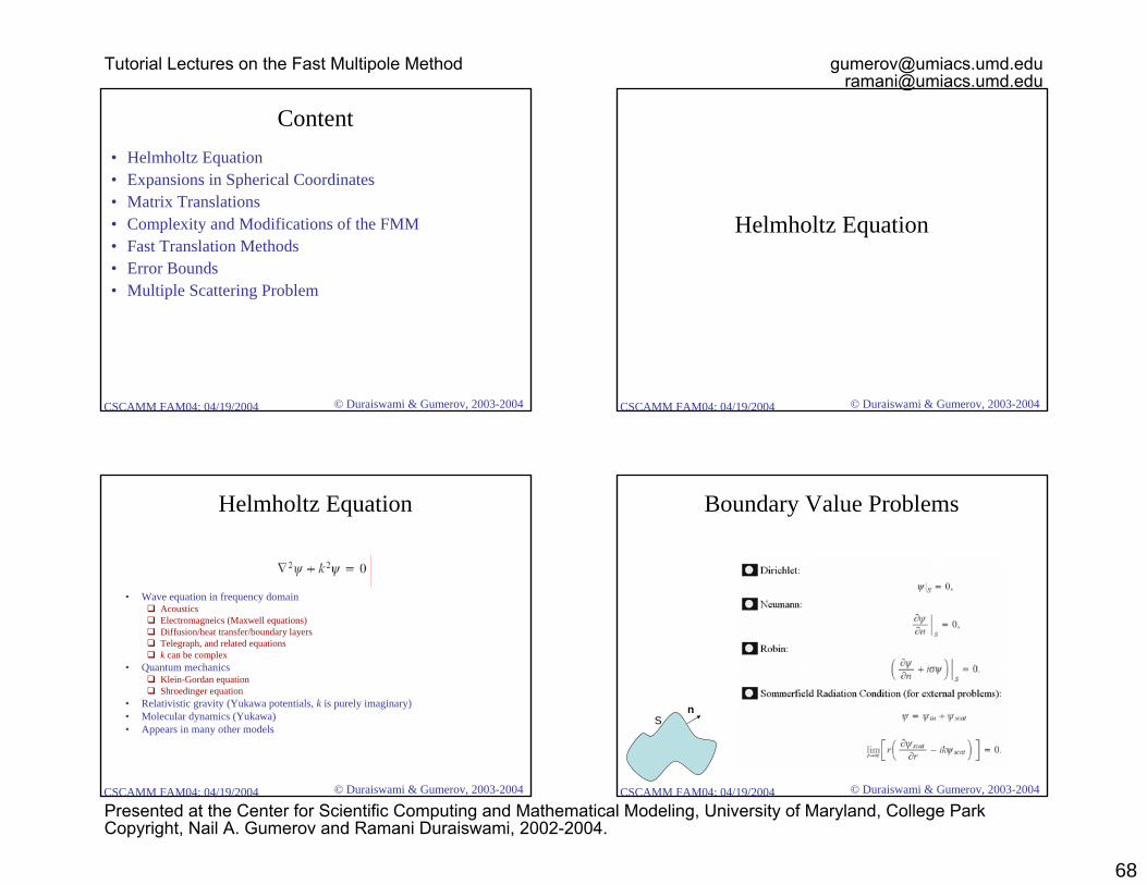
68
© Duraiswami & Gumerov, 2003-2004CSCAMM FAM04: 04/19/2004
Content• Helmholtz Equation• Expansions in Spherical Coordinates• Matrix Translations• Complexity and Modifications of the FMM• Fast Translation Methods• Error Bounds• Multiple Scattering Problem
© Duraiswami & Gumerov, 2003-2004CSCAMM FAM04: 04/19/2004
Helmholtz Equation
© Duraiswami & Gumerov, 2003-2004CSCAMM FAM04: 04/19/2004
Helmholtz Equation
• Wave equation in frequency domainAcousticsElectromagneics (Maxwell equations)Diffusion/heat transfer/boundary layersTelegraph, and related equationsk can be complex
• Quantum mechanicsKlein-Gordan equationShroedinger equation
• Relativistic gravity (Yukawa potentials, k is purely imaginary)• Molecular dynamics (Yukawa)• Appears in many other models
© Duraiswami & Gumerov, 2003-2004CSCAMM FAM04: 04/19/2004
Boundary Value Problems
nS
Tutorial Lectures on the Fast Multipole Method [email protected]@umiacs.umd.edu
Presented at the Center for Scientific Computing and Mathematical Modeling, University of Maryland, College ParkCopyright, Nail A. Gumerov and Ramani Duraiswami, 2002-2004.

69
© Duraiswami & Gumerov, 2003-2004CSCAMM FAM04: 04/19/2004
Green’s Function and Identity
nS Ω
© Duraiswami & Gumerov, 2003-2004CSCAMM FAM04: 04/19/2004
Distributions of Monopoles and Dipoles
nS Ω
© Duraiswami & Gumerov, 2003-2004CSCAMM FAM04: 04/19/2004
Expansions in Spherical Coordinates
© Duraiswami & Gumerov, 2003-2004CSCAMM FAM04: 04/19/2004
Spherical Basis Functions
x
y
z
O
x
y
z
O
x
y
z
Oθ
φ
r
rir
iθ
iφ
x
y
z
O
x
y
z
O
x
y
z
Oθ
φ
r
rir
iθ
iφ
Spherical Coordinates
Regular Basis Functions
Singular Basis Functions
Spherical Harmonics
Associated Legendre Functions
Spherical Bessel Functions
Spherical Hankel Functions of the First Kind
Tutorial Lectures on the Fast Multipole Method [email protected]@umiacs.umd.edu
Presented at the Center for Scientific Computing and Mathematical Modeling, University of Maryland, College ParkCopyright, Nail A. Gumerov and Ramani Duraiswami, 2002-2004.
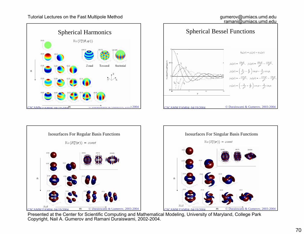
70
© Duraiswami & Gumerov, 2003-2004CSCAMM FAM04: 04/19/2004
Spherical Harmonics
n
m © Duraiswami & Gumerov, 2003-2004CSCAMM FAM04: 04/19/2004
Spherical Bessel Functions
© Duraiswami & Gumerov, 2003-2004CSCAMM FAM04: 04/19/2004
Isosurfaces For Regular Basis Functions
n
m © Duraiswami & Gumerov, 2003-2004CSCAMM FAM04: 04/19/2004
Isosurfaces For Singular Basis Functions
n
m
Tutorial Lectures on the Fast Multipole Method [email protected]@umiacs.umd.edu
Presented at the Center for Scientific Computing and Mathematical Modeling, University of Maryland, College ParkCopyright, Nail A. Gumerov and Ramani Duraiswami, 2002-2004.

71
© Duraiswami & Gumerov, 2003-2004CSCAMM FAM04: 04/19/2004
Expansions
Wave vector © Duraiswami & Gumerov, 2003-2004CSCAMM FAM04: 04/19/2004
Matrix Translations
© Duraiswami & Gumerov, 2003-2004CSCAMM FAM04: 04/19/2004
Reexpansions of Basis Functions
Reexpansion Matrices
rt
R S
Or
rt
R S
Or
© Duraiswami & Gumerov, 2003-2004CSCAMM FAM04: 04/19/2004
Recursive Computation of Reexpansion Matrices
|m|
n’
p-1
|m*|
02p-2-|m*| 2p-2p-1
n’
m m’(n’,m’,m+1)
(n’-1,m’-1,m) (n’+1,m’-1,m)
|m|
n’
p-1
|m*|
02p-2-|m*| 2p-2p-1
n’
m m’
n’
m m’(n’,m’,m+1)
(n’-1,m’-1,m) (n’+1,m’-1,m)
n n
|m’|
|m|
|m|
|m| |m’|
|s|
|m’| < |m| |m’| > |m|2p-2-|m|
p-1
p-12p-2-|m| 2p-2-|m’|
2p-2-|m’|
0 0
p-1-|m|+|m’|
p-1-|m’|+|m|
n’
n
(n’,n-1)
(n’-1,n)
(n’,n+1)
(n’+1,n)
n
(n’,n-1)
(n’-1,n)
(l,n+1)
(n’+1,n)
n’
n’ n’
p-1
p-1n n
|m’|
|m|
|m|
|m| |m’|
|s|
|m’| < |m| |m’| > |m|2p-2-|m|
p-1
p-12p-2-|m| 2p-2-|m’|
2p-2-|m’|
0 0
p-1-|m|+|m’|
p-1-|m’|+|m|
n’
n
(n’,n-1)
(n’-1,n)
(n’,n+1)
(n’+1,n)
n
(n’,n-1)
(n’-1,n)
(l,n+1)
(n’+1,n)
n’
n’ n’
p-1
p-1
p4 elements of the truncated reexpansion matrices can be computed for O(p4) operations recursively
Gumerov & Duraiswami,SIAM J. Sci. Stat. Comput.25(4), 1344-1381, 2003.
Tutorial Lectures on the Fast Multipole Method [email protected]@umiacs.umd.edu
Presented at the Center for Scientific Computing and Mathematical Modeling, University of Maryland, College ParkCopyright, Nail A. Gumerov and Ramani Duraiswami, 2002-2004.

72
© Duraiswami & Gumerov, 2003-2004CSCAMM FAM04: 04/19/2004
Translations
Ω1
Ω2
x*1
x*2R (R|R)
x R
Ωr(x*)
x*
(R|R)
y x*+tt
r
Ωr1(x*+t)
r1
xiΩ1
Ω2x*1
x*2
S
(S|S)
S
xi
x*x*+t
(S|S)
y
t
Ωr1(x*+t) Ωr(x*)
rr1
xiΩ1
x*1x*2
S
(S|S)
S
xi
x*
x*+t
(S|R)
y
t
Ωr1(x*+t)
r
r1
R|R S|S S|R
© Duraiswami & Gumerov, 2003-2004CSCAMM FAM04: 04/19/2004
Problem:
• For the Helmholtz equation absolute and uniform convergence can be achieved only for
p > ka. For large ka the FMM with constant p isvery expensive (comparable with straightforward methods);inaccurate (since keeps much larger number of terms than required, which causes numerical instabilities).
a
ExpansionDomain
D
2a=31/2D
© Duraiswami & Gumerov, 2003-2004CSCAMM FAM04: 04/19/2004
Model of Truncation Number Behavior for Fixed Error
p
ka0 ka*
p*
In the multilevel FMM we associate its own plwith each level l:
“Breakdown level”
Box size at level l© Duraiswami & Gumerov, 2003-2004CSCAMM FAM04: 04/19/2004
Complexity of Single Translation
Translation exponent
Tutorial Lectures on the Fast Multipole Method [email protected]@umiacs.umd.edu
Presented at the Center for Scientific Computing and Mathematical Modeling, University of Maryland, College ParkCopyright, Nail A. Gumerov and Ramani Duraiswami, 2002-2004.

73
© Duraiswami & Gumerov, 2003-2004CSCAMM FAM04: 04/19/2004
Spatially Uniform Data Distributions
Constant!© Duraiswami & Gumerov, 2003-2004CSCAMM FAM04: 04/19/2004
Complexity of the Optimized FMM for Fixed kD0 and Variable N
100000
1000000
1E+07
1E+08
1E+09
1E+10
1E+11
1E+12
1000 10000 100000 1000000Number of Sources
Num
ber o
f Mul
tiplic
atio
ns
nu=1, lb=2nu=1.5, lb=2nu=2, lb=2nu=1, lb=5nu=1.5, lb=5nu=2, lb=5
Straightforward, y=x2
3D Spatially Uniform Random Distribution
N=M
y=ax
© Duraiswami & Gumerov, 2003-2004CSCAMM FAM04: 04/19/2004
Optimum Level for Low Frequencies
0.00001
0.0001
0.001
0.01
0.1
1
10
100
2 3 4 5 6 7
Max Level of Space Subdivision
Num
ber o
f Mul
tiplic
atio
ns, x
10e1
1
N=M=10000003D Spatially Uniform Random Distribution
Direct SummationTranslation
Total
nu=1
1.5
2
2
1.5
1
© Duraiswami & Gumerov, 2003-2004CSCAMM FAM04: 04/19/2004
Volume Element Methods
Ns
wavelength
D0 = D0 k/(2π) wavelengths = N1/3 sourcesCritical Translation Exponent!
computational domain
Tutorial Lectures on the Fast Multipole Method [email protected]@umiacs.umd.edu
Presented at the Center for Scientific Computing and Mathematical Modeling, University of Maryland, College ParkCopyright, Nail A. Gumerov and Ramani Duraiswami, 2002-2004.

74
© Duraiswami & Gumerov, 2003-2004CSCAMM FAM04: 04/19/2004
What Happens if Truncation Number is Constant for All Levels?
“Catastrophic Disaster of the FMM”
© Duraiswami & Gumerov, 2003-2004CSCAMM FAM04: 04/19/2004
Surface Data Distributions
Critical Translation Exponent!
Boundary Element Methods:
© Duraiswami & Gumerov, 2003-2004CSCAMM FAM04: 04/19/2004
Optimum Level of Space Subdivision
0
1
2
3
4
5
6
7
8
1000 10000 100000 1000000Number of Sources
Opt
imum
Max
Lev
el
nu=1nu=1.5nu=2
lb=20
1
2
3
4
5
6
7
8
1000 10000 100000 1000000Number of Sources
Opt
imum
Max
Lev
el
nu=1nu=1.5nu=2
lb=5
lb=2 lb=5
© Duraiswami & Gumerov, 2003-2004CSCAMM FAM04: 04/19/2004
Performance of the MLFMM for Surface Data Distributions
100000
1000000
1E+07
1E+08
1E+09
1E+10
1E+11
1E+12
1000 10000 100000 1000000Number of Sources
Num
ber o
f Mul
tiplic
atio
ns
nu=1, lb=2nu=1.5, lb=2nu=2, lb=2nu=1, lb=5nu=1.5, lb=5nu=2, lb=5
Straightforward, y=x2
Uniform Random Distributionover a Sphere Surface
N=M
y=ax
Tutorial Lectures on the Fast Multipole Method [email protected]@umiacs.umd.edu
Presented at the Center for Scientific Computing and Mathematical Modeling, University of Maryland, College ParkCopyright, Nail A. Gumerov and Ramani Duraiswami, 2002-2004.

75
© Duraiswami & Gumerov, 2003-2004CSCAMM FAM04: 04/19/2004
Effective Dimensionality of the Problem
Computational domain
1 cube
8 cubes© Duraiswami & Gumerov, 2003-2004CSCAMM FAM04: 04/19/2004
Fast Translation Methods
© Duraiswami & Gumerov, 2003-2004CSCAMM FAM04: 04/19/2004
Translation Methods• O(p5): Matrix Translation with Computation of Matrix Elements Based on Clebsch-
Gordan Coefficients;• O(p4) (Low Asymptotic Constant): Matrix Translation with Recursive Computation of
Matrix Elements• O(p3) (Low Asymptotic Constants):
Rotation-Coaxial Translation Decomposition with Recursive Computation of Matrix Elements;Sparse Matrix Decomposition;
• O(p2logβp)Rotation-Coaxial Translation Decomposition with Structured Matrices for Rotation and Fast Legendre Transform for Coaxial Translation;Translation Matrix Diagonalization with Fast Spherical Transform;Asymptotic Methods;Diagonal Forms of Translation Operators with Spherical Filtering.
© Duraiswami & Gumerov, 2003-2004CSCAMM FAM04: 04/19/2004
O(p3) Methods
Tutorial Lectures on the Fast Multipole Method [email protected]@umiacs.umd.edu
Presented at the Center for Scientific Computing and Mathematical Modeling, University of Maryland, College ParkCopyright, Nail A. Gumerov and Ramani Duraiswami, 2002-2004.

76
© Duraiswami & Gumerov, 2003-2004CSCAMM FAM04: 04/19/2004
Rotation - Coaxial Translation Decomposition (Complexity O(p3))
z
y
y
xx
yx
z
yx
z
zp4
p3p3
p3
z
y
y
xx
yx
zyx
z
yx
z
zp4
p3p3
p3
From the group theory follows that general translation can be reduced to
0.01
0.1
1
10
10 100
Truncation Number, p
CP
U T
ime
(s)
Full Matrix Translation
Rotational-Coaxial Translation Decomposition
y=ax4
y=bx3
kt=86
© Duraiswami & Gumerov, 2003-2004CSCAMM FAM04: 04/19/2004
Sparse Matrix Decomposition
Matrix-vector products with these matrices computed recursively
© Duraiswami & Gumerov, 2003-2004CSCAMM FAM04: 04/19/2004
O(p2logβp) Methods
© Duraiswami & Gumerov, 2003-2004CSCAMM FAM04: 04/19/2004
Fast Rotation Transform
Euler angles
Diagonal matrices
Diagonal matrices
Block-Toeplitz matrices
Complexity: O(p2logp)
Tutorial Lectures on the Fast Multipole Method [email protected]@umiacs.umd.edu
Presented at the Center for Scientific Computing and Mathematical Modeling, University of Maryland, College ParkCopyright, Nail A. Gumerov and Ramani Duraiswami, 2002-2004.

77
© Duraiswami & Gumerov, 2003-2004CSCAMM FAM04: 04/19/2004
Fast Coaxial Translation
Diagonal matricesLegendre andtransposed Legendre matrices
Fast multiplication of the Legendre and transposed Legendre matrices can be performed via the forward and inverse FAST LEGENDRE TRANSFORM (FLT) with complexity O(p2log2p)
Healy et al Advances in Computational Mathematics 21: 59-105, 2004.© Duraiswami & Gumerov, 2003-2004CSCAMM FAM04: 04/19/2004
Diagonalization of General Translation Operator
Diagonal matricesMatrices for the forward and inverse and Spherical Transform
FAST SPHERICAL TRANSFORM (FST) can be performed with complexity O(p2log2p)
Healy et al Advances in Computational Mathematics 21: 59-105, 2004.
© Duraiswami & Gumerov, 2003-2004CSCAMM FAM04: 04/19/2004
Method of Signature Function(Diagonal Forms of the Translation Operator)
Regular Solution
Singular Solution
© Duraiswami & Gumerov, 2003-2004CSCAMM FAM04: 04/19/2004
Final Summation and Initial Expansion
Tutorial Lectures on the Fast Multipole Method [email protected]@umiacs.umd.edu
Presented at the Center for Scientific Computing and Mathematical Modeling, University of Maryland, College ParkCopyright, Nail A. Gumerov and Ramani Duraiswami, 2002-2004.

78
© Duraiswami & Gumerov, 2003-2004CSCAMM FAM04: 04/19/2004
The FMM with Band-Unlimited Signature Functions (O(p2) method)
0.1
1
10
100
1000
10000
1000 10000 100000 1000000Number of Sources
CP
U T
ime
(s)
y = ax 2
y = bx
Straightforward
FMM
O(p )3
O(p )2
O(p )+err bound2
kD =10, M=N,Spatially Uniform Random Distributions
0
Pre-Set StepO(p )2
O(p )3
© Duraiswami & Gumerov, 2003-2004CSCAMM FAM04: 04/19/2004
Deficiencies• Low Frequencies;• High Frequencies;• Constant p;• Instabilities after two or three levels of translations.
© Duraiswami & Gumerov, 2003-2004CSCAMM FAM04: 04/19/2004
Methods to Fix:• Use of Band-limited functions;• Error control via band-limits;• Requires filtering procedures (complexity O(p2log2p) or O(p2logp))
with large asymptotic constants;• The length of the representation is changed via
interpolation/anterpolation procedures.
© Duraiswami & Gumerov, 2003-2004CSCAMM FAM04: 04/19/2004
Error Bounds
Tutorial Lectures on the Fast Multipole Method [email protected]@umiacs.umd.edu
Presented at the Center for Scientific Computing and Mathematical Modeling, University of Maryland, College ParkCopyright, Nail A. Gumerov and Ramani Duraiswami, 2002-2004.

79
© Duraiswami & Gumerov, 2003-2004CSCAMM FAM04: 04/19/2004
Source Expansion Errors
rs
r
ab
rs
r
ab0 0
rs
r
ab
rs
r
ab0 0
© Duraiswami & Gumerov, 2003-2004CSCAMM FAM04: 04/19/2004
Approximation of the Error
© Duraiswami & Gumerov, 2003-2004CSCAMM FAM04: 04/19/2004
We proved that for source summation problems the truncation numbers can be selected based on the above
chart when using translations with rectangularlytruncated matrices
r
ab0
rs
a/2tb/2
r
ab0
rs
a/2tb/2
ra
b
0rs
ta
ra
b
0rs
ta
r
ab
rs
a/2t0
r
ab
rs
a/2t0
S|S S|R R|R
© Duraiswami & Gumerov, 2003-2004CSCAMM FAM04: 04/19/2004
Low Frequency FMM Error
a
b
O
A
B
ab
C
B
a
O
A
Q
R|R, S|S S|R
a
b
O
A
B
ab
C
B
a
O
A
Qa
b
O
A
B
ab
C
B
a
O
A
Q
R|R, S|S S|R
Tutorial Lectures on the Fast Multipole Method [email protected]@umiacs.umd.edu
Presented at the Center for Scientific Computing and Mathematical Modeling, University of Maryland, College ParkCopyright, Nail A. Gumerov and Ramani Duraiswami, 2002-2004.

80
© Duraiswami & Gumerov, 2003-2004CSCAMM FAM04: 04/19/2004
High Frequency FMM Error
© Duraiswami & Gumerov, 2003-2004CSCAMM FAM04: 04/19/2004
Multiple Scattering Problem
© Duraiswami & Gumerov, 2003-2004CSCAMM FAM04: 04/19/2004
Problem
Boundary Conditions:
100 random spheres 1000 random spheres100 random spheres 1000 random spheres © Duraiswami & Gumerov, 2003-2004CSCAMM FAM04: 04/19/2004
Scattered Field DecompositionT-Matrix Method
Expansion Coefficients
Singular Basis Functions Hankel Functions
Spherical Harmonics
Vector Form:
dot product
Tutorial Lectures on the Fast Multipole Method [email protected]@umiacs.umd.edu
Presented at the Center for Scientific Computing and Mathematical Modeling, University of Maryland, College ParkCopyright, Nail A. Gumerov and Ramani Duraiswami, 2002-2004.

81
© Duraiswami & Gumerov, 2003-2004CSCAMM FAM04: 04/19/2004
Solution of Multiple Scattering Problem
T-Matrix Method
4
2
1
6
53
Incident Wave
Scattered Wave
Coupled System of Equations:
(S|R)-TranslationMatrix
“Effective” Incident Field
© Duraiswami & Gumerov, 2003-2004CSCAMM FAM04: 04/19/2004
Reflection Method & Krylov Subspace Method (GMRES)
Reflection (Simple Iteration) Method:
General Formulation (used in GMRES)
Iterative Methods
© Duraiswami & Gumerov, 2003-2004CSCAMM FAM04: 04/19/2004
100 random spheres (MLFMM)ka=1.6 ka=4.8ka=2.8
R G B
© Duraiswami & Gumerov, 2003-2004CSCAMM FAM04: 04/19/2004
Surface Potential Imaging
Tutorial Lectures on the Fast Multipole Method [email protected]@umiacs.umd.edu
Presented at the Center for Scientific Computing and Mathematical Modeling, University of Maryland, College ParkCopyright, Nail A. Gumerov and Ramani Duraiswami, 2002-2004.

82
© Duraiswami & Gumerov, 2003-2004CSCAMM FAM04: 04/19/2004
Performance Test
1
10
100
1000
10000
100000
10 100 1000 10000 100000Number of Scatterers
CP
U T
ime
(s)
Volume Fraction = 0.2, ka=0.5
Periodically-Random Spatial Distributionof Spheres of Equal Size
Reflection +FMMStraightforward
y=cx3
y=ax
Reflection+Direct
y=bx2
© Duraiswami & Gumerov, 2003-2004CSCAMM FAM04: 04/19/2004
Computable Problems on Desktop PC
MLFMM
Met
hod
Number of Scatterers101 102 103100 104 105
BEM
Multipole Straightforward
Multipole Iterative
MLFMM
Also strongly depends on ka !
© Duraiswami & Gumerov, 2003-2004CSCAMM FAM04: 04/19/2004
More About This Problemin Our Talk Next Week
Tutorial Lectures on the Fast Multipole Method [email protected]@umiacs.umd.edu
Presented at the Center for Scientific Computing and Mathematical Modeling, University of Maryland, College ParkCopyright, Nail A. Gumerov and Ramani Duraiswami, 2002-2004.