An Introduction to Evolutionary Multiobjective Optimization

An Introduction to EvolutionaryMultiobjective Optimization

Carlos A. Coello Coello

CINVESTAV-IPN

Departamento de Computacion

Av. Instituto Politecnico Nacional No. 2508

Col. San Pedro Zacatenco

Mexico, D. F. 07360, MEXICO

email: [email protected]

1

Motivation

Most problems in nature have several (possibly conflicting)objectives to be satisfied. Many of these problems are frequentlytreated as single-objective optimization problems by transformingall but one objective into constraints.

2

What is a multiobjective optimization problem?

The Multiobjective Optimization Problem (MOP) (alsocalled multicriteria optimization, multiperformance or vectoroptimization problem) can be defined (in words) as the problem offinding (Osyczka, 1985):

a vector of decision variables which satisfies constraints andoptimizes a vector function whose elements represent theobjective functions. These functions form a mathematicaldescription of performance criteria which are usually inconflict with each other. Hence, the term “optimize” meansfinding such a solution which would give the values of allthe objective functions acceptable to the decision maker.

3

A Formal Definition

The general Multiobjective Optimization Problem (MOP) can beformally defined as:

Find the vector ~x∗ = [x∗1, x∗2, . . . , x

∗n]T which will satisfy the m

inequality constraints:

gi(~x) ≤ 0 i = 1, 2, . . . ,m (1)

the p equality constraints

hi(~x) = 0 i = 1, 2, . . . , p (2)

and will optimize the vector function

~f(~x) = [f1(~x), f2(~x), . . . , fk(~x)]T (3)

4

What is the notion of optimum

in multiobjective optimization?

Having several objective functions, the notion of “optimum”changes, because in MOPs, we are really trying to find goodcompromises (or “trade-offs”) rather than a single solution as inglobal optimization. The notion of “optimum” that is mostcommonly adopted is that originally proposed by Francis YsidroEdgeworth in 1881.

5

What is the notion of optimum

in multiobjective optimization?

This notion was later generalized by Vilfredo Pareto (in 1896).Although some authors call Edgeworth-Pareto optimum to thisnotion, we will use the most commonly accepted term: Paretooptimum.

6

Definition of Pareto Optimality

We say that a vector of decision variables ~x∗ ∈ F is Pareto optimalif there does not exist another ~x ∈ F such that fi(~x) ≤ fi(~x∗) forall i = 1, . . . , k and fj(~x) < fj(~x∗) for at least one j.

7

Definition of Pareto Optimality

In words, this definition says that ~x∗ is Pareto optimal if thereexists no feasible vector of decision variables ~x ∈ F which woulddecrease some criterion without causing a simultaneous increase inat least one other criterion. Unfortunately, this concept almostalways gives not a single solution, but rather a set of solutionscalled the Pareto optimal set. The vectors ~x∗ correspoding to thesolutions included in the Pareto optimal set are callednondominated. The plot of the objective functions whosenondominated vectors are in the Pareto optimal set is called thePareto front.

8

Sample Pareto Front

0

0.005

0.01

0.015

0.02

0.025

0.03

0.035

0.04

1200 1400 1600 1800 2000 2200 2400 2600 2800

f2

f1

3333333333333333333333333333333333333333333333333333333333333333333333333333333333333333333333333333333333333333333333333333333333333333333333333333333333333333333333333333333333333333333333333333333333333333333333333333333333333333333333333333333333333333333333333333333333333333333333333333333333333333333333333333333333333333333333333333333333333333333333333333333333333333333333333333333333333333333333333333333333333333333333333333333333333333333333333333333333333333333333333333333333333333333333333333333333333333333333333333333333333333333

9

Some Historical Highlights

As early as 1944, John von Neumann and Oskar Morgensternmentioned that an optimization problem in the context of a socialexchange economy was “a peculiar and disconcerting mixture ofseveral conflicting problems” that was “nowhere dealt with inclassical mathematics”.

10


In 1951 Tjalling C. Koopmans edited a book called ActivityAnalysis of Production and Allocation, where the concept of“efficient” vector was first used in a significant way.

11


The origins of the mathematical foundations of multiobjectiveoptimization can be traced back to the period that goes from 1895to 1906. During that period, Georg Cantor and Felix Hausdorff laidthe foundations of infinite dimensional ordered spaces.

12


Cantor also introduced equivalence classes and stated the firstsufficient conditions for the existence of a utility function.Hausdorff also gave the first example of a complete ordering.

13


However, it was the concept of vector maximum problem introducedby Harold W. Kuhn and Albert W. Tucker (1951) which mademultiobjective optimization a mathematical discipline on its own.

14


However, multiobjective optimization theory remained relativelyundeveloped during the 1950s. It was until the 1960s that thefoundations of multiobjective optimization were consolidated andtaken seriously by pure mathematicians when Leonid Hurwiczgeneralized the results of Kuhn & Tucker to topological vectorspaces.

15

Antecedentes Historicos

Perhaps the most important research outcome from the 1950s wasthe development of Goal Programming, which was originallyintroduced by Abraham Charnes and William Wager Cooper in1957.

16


The application of multiobjective optimization to domains outsideeconomics began with the work by Koopmans (1951) in productiontheory and with the work of Marglin (1967) in water resourcesplanning.

17


The first engineering application reported in the literature was apaper by Zadeh in the early 1960s. However, the use ofmultiobjective optimization became generalized until the 1970s.

18

Current State of the Area

Currently, there are over 30 mathematical programming techniquesfor multiobjective optimization. However, these techniques tend togenerate elements of the Pareto optimal set one at a time.Additionally, most of them are very sensitive to the shape of thePareto front (e.g., they do not work when the Pareto front isconcave or when the front is disconnected).

19

Why Evolutionary Algorithms?

Evolutionary algorithms seem particularly suitable to solvemultiobjective optimization problems, because they dealsimultaneously with a set of possible solutions (the so-calledpopulation). This allows us to find several members of the Paretooptimal set in a single run of the algorithm, instead of having toperform a series of separate runs as in the case of the traditionalmathematical programming techniques. Additionally, evolutionaryalgorithms are less susceptible to the shape or continuity of thePareto front (e.g., they can easily deal with discontinuous orconcave Pareto fronts), whereas these two issues are a real concernfor mathematical programming techniques.

20

Historical Development

The potential of evolutionary algorithms in multiobjectiveoptimization was hinted by Rosenberg in the 1960s, but the firstactual implementation was produced in the mid-1980s (Schaffer,1984). The first scheme to incorporate user’s preferences into amulti-objective evolutionary algorithm (MOEA) was proposed inthe early 1990s (Tanaka, 1992). During ten years, the field remainpractically inactive, but it started growing in the mid-1990s, inwhich several techniques and applications were developed.

21

Evolutionary Algorithms

We can consider, in general, two main types of MOEAs:

1. Algorithms that do not incorporate the concept of Paretodominance in their selection mechanism (e.g., approaches thatuse linear aggregating functions).

2. Algorithms that rank the population based on Paretodominance. For example, MOGA, NSGA, NPGA, etc.

22

Evolutionary Algorithms

Historically, we can consider the existence of two main generationsof MOEAs:

1. First Generation: Characterized by the use of Paretoranking and niching (or fitness sharing). Relatively simplealgorithms. Other (more rudimentary) approaches were alsodeveloped (e.g., linear aggregating functions). It is also worthmentioning VEGA, which is a population-based (notPareto-based) approach.

2. Second Generation: The concept of elitism is introduced intwo main forms: using (µ+ λ) selection and using a secondary(external) population.

23

Representative MOEAs (First Generation)

• Aggregating Functions

• VEGA

• MOGA

• NSGA

• NPGA & NPGA 2

24

Aggregating Functions

• These techniques are called “aggregating functions” becausethey combine (or “aggregate”) all the objectives into a singleone. We can use addition, multiplication or any othercombination of arithmetical operations.

• Oldest mathematical programming method, since aggregatingfunctions can be derived from the Kuhn-Tucker conditions fornondominated solutions.

25

Aggregating Functions

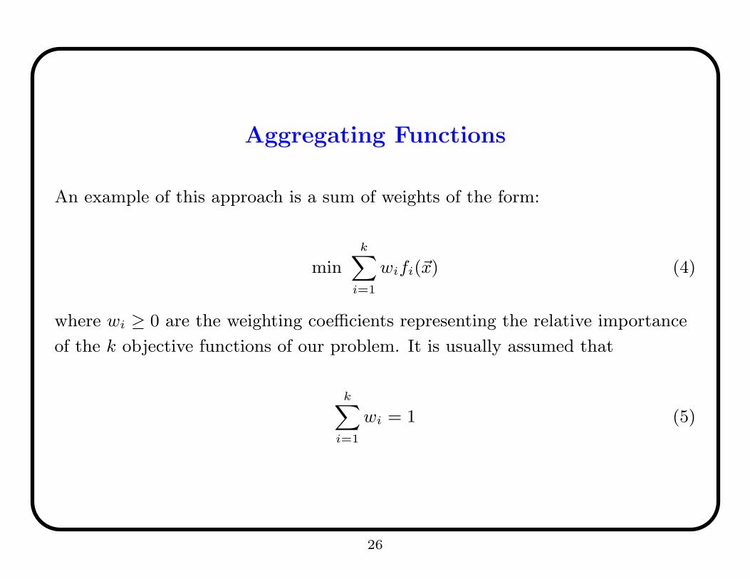
An example of this approach is a sum of weights of the form:

mink∑

i=1

wifi(~x) (4)

where wi ≥ 0 are the weighting coefficients representing the relative importance

of the k objective functions of our problem. It is usually assumed that

k∑

i=1

wi = 1 (5)

26

Advantages and Disadvantages

• Easy to implement

• Efficient

• Linear combinations of weights do not work when the Paretofront is concave, regardless of the weights used (Das, 1997).Note however, that the weights can be generated in such a waythe the Pareto front is rotated (Jin et al., 2001). In this lastcase, concave Pareto fronts can be efficiently generated.

27

Sample Applications

• Design of DSP systems (Arslan, 1996).

• Water quality control (Garrett, 1999).

• System-level synthesis (Blickle, 1996).

• Design of optical filters for lamps (Eklund, 1999).

28

Vector Evaluated Genetic Algorithm (VEGA)

• Proposed by Schaffer in the mid-1980s (1984,1985).

• It uses subpopulations that optimize each objective separately.The concept of Pareto optimum is not directly incorporatedinto the selection mechanism of the GA.

29

VEGA

Individual 1

Individual 2

Individual N

Individual 3

Sub−popu− lation 1

lation 2Sub−popu−

Sub−popu−lation M

Individual 1

Individual 2

Individual 3

Individual N Individual N

Individual 3

Individual 2

Individual 1

Sub−popu−lation 3

Create

Sub−popu−lations

Generation (t)

Initial PopulationSize N

M sub−populationsare created

Shuffle

entirepopulation

Individuals are nowmixed

Apply

geneticoperators

Generation (t+1)

Start all over again

30


• Efficient and easy to implement.

• It doesn’t have an explicit mechanism to maintain diversity. Itdoesn’t necessarily produce nondominated vectors.

31

Sample Applications

• Aerodynamic optimization (Rogers, 2000).

• Combinational circuit design at the gate-level (Coello, 2000).

• Design multiplierless IIR filters (Wilson, 1993).

• Groundwater pollution containment (Ritzel, 1994).

32

Multi-Objective Genetic Algorithm (MOGA)

• Proposed by Fonseca and Fleming (1993).

• The approach consists of a scheme in which the rank of acertain individual corresponds to the number of individuals inthe current population by which it is dominated.

• It uses fitness sharing and mating restrictions.

33


• Efficient and relatively easy to implement.

• Its performance depends on the appropriate selection of thesharing factor.

• MOGA was the most popular first-generation MOEA and itnormally outperformed all of its contemporary competitors.

34

Some Applications

• Fault diagnosis (Marcu, 1997).

• Control system design (Chipperfield 1995; Whidborne, 1995;Duarte, 2000).

• Design of antennas (Thompson, 2001).

• System-level synthesis (Dick, 1998).

• Rehabilitation of a water distribution system (Cheung, 2003).

• Forest management (Ducheyne, 2003)

35


• Relatively easy to implement.

• Seems to be very sensitive to the value of the sharing factor.

36

Sample Applications

• Water quality control (Reed et al., 2001).

• Design of control systems (Blumel, 2001).

• Constellation design (Mason, 1999).

• Computational fluid dynamics (Marco, 1999).

• Chemical engineering (Kasat, 2003).

37

Niched-Pareto Genetic Algorithm (NPGA)

• Proposed by Jeffrey Horn et al. (1993,1994).

• It uses a tournament selection scheme based on Pareto dominance. Two

individuals randomly chosen are compared against a subset from the entire

population (typically, around 10% of the population). When both

competitors are either dominated or nondominated (i.e., when there is a

tie), the result of the tournament is decided through fitness sharing in the

objective domain (a technique called equivalent class sharing is used in

this case).

38


• Easy to implement.

• Efficient because does not apply Pareto ranking to the entirepopulation.

• It seems to have a good overall performance.

• Besides requiring a sharing factor, it requires anotherparameter (tournament size).

39

Sample Applications

• Analysis of experimental spectra (Golovkin, 2000).

• Feature selection (Emmanouilidis, 2000).

• Fault-tolerant systems design (Schott, 1995).

• Road systems design (Haastrup & Pereira, 1997).

40

NPGA 2

Erickson et al. (2001) proposed the NPGA 2, which uses Paretoranking but keeps tournament selection (solving ties through fitnesssharing as in the original NPGA).

Niche counts in the NPGA 2 are calculated using individuals in thepartially filled next generation, rather than using the currentgeneration. This is called continuously updated fitness sharing, andwas proposed by Oei et al. (1991).

41

Sample Applications

• Design of groundwater remediation systems (Erickson et al.,2001).

42

Representative MOEAs (Second Generation)

• SPEA and SPEA2

• NSGA-II

• PAES, PESA and PESA II

• MOMGA and MOMGA II

• The microGA for multiobjective optimization and themicroGA2

43

The Strength Pareto

Evolutionary Algorithm (SPEA)

SPEA was introduced by Zitzler & Thiele (1999). It uses anexternal archive containing nondominated solutions previouslyfound. SPEA computes a strength value similar to the rankingvalue used by MOGA. A clustering technique called “averagelinkage method” is used to keep diversity.

44

Sample Applications

• Exploration of trade-offs of software implementations for DSPalgorithms (Zitzler, 1999)

• Treatment planning (Petrovski, 2001)

• Allocation in radiological facilities (Lahanas, 2001)

• Atrial disease diagnosis (de Toro, 2003).

• Rehabilitation of a water distribution system (Cheung, 2003).

45

The Strength Pareto

Evolutionary Algorithm 2 (SPEA2)

A revised version of SPEA has been recently proposed: SPEA2(Zitzler, 2001). SPEA2 has three main differences with respect toits predecessor: (1) it incorporates a fine-grained fitness assignmentstrategy which takes into account for each individual the number ofindividuals that dominate it and the number of individuals bywhich it is dominated; (2) it uses a nearest neighbor densityestimation technique which guides the search more efficiently, and(3) it has an enhanced archive truncation method that guaranteesthe preservation of boundary solutions.

46

Sample Applications

• Control code size and reduce bloat in genetic programming(Bleuler, 2001).

• Airfoil design (Willmes, 2003).

47

The Nondominated Sorting

Genetic Algorithm II (NSGA-II)

Deb et al. (2000,2002) proposed a new version of theNondominated Sorting Genetic Algorithm (NSGA), calledNSGA-II, which is more efficient (computationally speaking), ituses elitism and a crowded comparison operator that keepsdiversity without specifying any additional parameters.

48

Sample Applications

• Shape optimization (Deb, 2001).

• Safety systems design (Greiner, 2003).

• Polymer extrusion (Gaspar-Cunha, 2003).

• Water quality management (Dorn, 2003).

• Intensity modulated beam radiation therapy (Lahanas, 2003).

49

The Pareto Archived Evolution Strategy (PAES)

PAES was introduced by Knowles & Corne (2000). It uses a (1+1)evolution strategy together with an external archive that records allthe nondominated vectors previously found. PAES uses anadaptive grid to maintain diversity.

50

PAES (Adaptive Grid)

��

��

��

��

��

��

��

��

��

��

��

��

��

��

��

��

��

��

A

B

C

DE

F

GH

IJ

K

LM

N

7

6

5

4

3

2

1

0

0 1 2 3 4 5 6 7f1

f2Size

of function 1

Size

of fu

nctio

n 2Individual with the highest

fitness in function 1 andmaximum fitness in function 2

Individual with the highestfitness in function 2 and

maximum fitness in function 1

Hypercube

nSubdivs = 7

nSubdivs = 7

extra room

corresponding componentto cover in the

function 1

Space that we need

51

Sample Applications

• Off-line routing problem (Knowles, 1999)

• Adaptive distributed database management problem (Knowles,2000)

52

The Pareto Envelope-based

Selection Algorithm (PESA)

PESA was proposed by Corne et al. (2000). This approach uses a small

internal population and a larger external (or secondary) population.

PESA uses the same hyper-grid division of phenotype (i.e., objective

funcion) space adopted by PAES to maintain diversity. However, its

selection mechanism is based on the crowding measure used by the

hyper-grid previously mentioned. This same crowding measure is used to

decide what solutions to introduce into the external population (i.e., the

archive of nondominated vectors found along the evolutionary process).

53

Sample Applications

• Telecommunications problems (Corne et al., 2000).

54

The Pareto Envelope-based

Selection Algorithm-II (PESA-II)

PESA-II (Corne et al., 2001) is a revised version of PESA in whichregion-based selection is adopted. In region-based selection, theunit of selection is a hyperbox rather than an individual. Theprocedure consists of selecting (using any of the traditionalselection techniques) a hyperbox and then randomly select anindividual within such hyperbox.

55

Sample Applications

• Telecommunications problems (Corne et al., 2001).

56

The Multi-Objective Messy

Genetic Algorithm (MOMGA)

MOMGA was proposed by Van Veldhuizen and Lamont (2000).This is an attempt to extend the messy GA to solve multiobjectiveoptimization problems.

MOMGA consists of three phases: (1) Initialization Phase, (2)Primordial Phase, and (3) Juxtapositional Phase. In theInitialization Phase, MOMGA produces all building blocks of acertain specified size through a deterministic process known aspartially enumerative initialization. The Primordial Phaseperforms tournament selection on the population and reduces thepopulation size if necessary. In the Juxtapositional Phase, themessy GA proceeds by building up the population through the useof the cut and splice recombination operator.

57

Sample Applications

• Design of controllers (Herreros, 2000).

• Traditional benchmarks (Van Veldhuizen & Lamont, 2000).

58

The Multi-Objective Messy

Genetic Algorithm-II (MOMGA-II)

Zydallis et al. (2001) proposed MOMGA-II. In this case, theauthors extended the fast-messy GA, which consists of threephases: (1) Initialization Phase, (2) Building Block Filtering, and(3) Juxtapositional Phase. Its main difference with respect to theoriginal messy GA is in the two first phases. The InitializationPhase utilizes probabilistic complete initialization which creates acontrolled number of building block clones of a specified size. TheBuilding Block Filtering Phase reduces the number of buildingblocks through a filtering process and stores the best buildingblocks found. The Juxtapositional Phase is the same as in theMOMGA.

59

Sample Applications

• Traditional benchmarks (Zydallis et al., 2001).

60

The Micro Genetic Algorithm

for Multiobjective Optimization

Proposed by Coello and Toscano-Pulido [2001]. A micro genetic

algorithms uses a population size ≤ 5 individuals. The key aspect of the

microGA is the use of a reinitialization process once nominal convergence

is reached. The microGA for multiobjective optimization uses 3 forms of

elitism and the adaptive grid from PAES.

61

The Micro Genetic Algorithm

InicialPopulation

Nominal

Selection

Crossover

Mutation

Elitism

NewPopulation

Convergence?

Filter

External Memory

cyclemicro−GA

N

Y

Non−ReplaceableReplaceable

Population Memory

RandomPopulation

Fill inboth parts

of the populationmemory

62

Sample Applications

• Supersonic jet design (Chung et al., 2003).

• Structural design (Coello, 2002).

• Hardware/Software Partitioning of UML Specifications(Fornaciari, 2003).

63

The Micro Genetic Algorithm2 (µGA2)

Proposed by Toscano Pulido & Coello [2003]. The main motivation of

the µGA2 was to eliminate the 8 parameters required by the original

algorithm. The muGA2 uses on-line adaption mechanisms that make

unnecessary the fine-tuning of any of its parameters. The muGA2 can

even decide when to stop (no maximum number of generations has to be

provided by the user). The only parameter that it requires is the size of

external archive (although there is obviously a default value for this

parameter).

64

The Micro Genetic Algorithm2 (µGA2)

AdaptiveMicro

GA

AdaptiveMicro

GA

AdaptiveMicro

GA

Select crossover operators

External Memory

Compare results andrank the subpopulations

Select the population memoriesfor the Adaptive micro−GAs

Initialize population memories

Initialize crossover operators

N

Y

Convergence?

65

Sample Applications

Since it is a very recent algorithm, so far it has been used only withtraditional benchmarks.

66

Current Trends in MOEAs

• After great success for over 10 years, first generation MOEAshave finally started to become obsolete in the literature(NSGA, NPGA, MOGA and VEGA).

• From the late 1990s, second generation MOEAs are consideredthe state-of-the-art in evolutionary multiobjective optimization(e.g., SPEA, SPEA2, NSGA-II, MOMGA, MOMGA-II, PAES,PESA, PESA II, microGA, etc.).

67

Current Trends in MOEAs

• Second generation MOEAs emphasize computational efficiency.One of the main goals is to find ways around the computationalcomplexity of Pareto ranking (O(kM2), where k is the numberof objective functions and M is the population size) andaround the computational cost of niching (O(M2)).

• Largely ignored by a significant number of researchers,non-Pareto MOEAs are still popular in Operations Research(e.g., in multiobjective combinatorial optimization), where theyhave been very successful.

68

Current state of the literature (mid of 2007)

67 83 84 85 86 87 88 89 90 91 92 93 94 95 96 97 98 99 00 01 02 03 04 05 06 070

50

100

150

200

250

300

350

400

Publication Year

Num

ber o

f Pub

licat

ions

69

Maintaining Diversity

An important aspect of MOEAs is to be able to maintain diversityin the population. For many years, fitness sharing was the mainmechanism adopted for this purpose (Goldberg & Richardson,1987). The idea of fitness sharing is to subdivide the populationinto several subpopulations based on the similarity amongindividuals. Note that when referring to MOEAs, “similarity” canbe measured in the space of the decision variables (either encodedor decoded) or in the space of the objective functions.

70


Fitness sharing is defined in the following way:

φ(dij) =

1−(

dijσshare

)α

, dij < σshare

0, otherwise(6)

71


In the expression of the previous slide: α = 1, dij indicates thedistance between solutions i and j (in any space defined), andσshare is a parameter (or threshold) that defines the size of a nicheor neighborhood. Any solutions within this distance will beconsidered as part of the same niche. The fitness of an individual iis computed using:

fsi =fi

∑Mj=1 φ(dij)

(7)

where M is the number of individuals located in the neighborhood(or niche) of the i-th individual.

72


Several other schemes are possible to maintain diversity and toencourage a good spread of solutions. For example:

• Crowding techniques.

• Clustering techniques.

• The adaptive grid of PAES (Knowles & Corne, 2000).

• The use of the concept of entropy.

73


Other authors have also proposed the use of mating restrictions(which operate with a parameter σmate similar to σshare). Thereare also several other mechanisms to maintain diversity (see forexample Mahfoud’s PhD thesis), although few of them have beenadopted with MOEAs. Note however, that there are no standardguidelines regarding the suitability of any of these mechanisms forany specific application or algorithm and their use is based on thepreferences of the user.

74

Theory

The most important theoretical work related to EMOO hasconcentrated on the following issues:

• Studies of convergence towards the Pareto optimum set(Rudolph, 1998, 2000, 2001; Hanne 2000,2000a; VanVeldhuizen, 1998).

• Ways to compute appropriate sharing factors (or niche sizes)(Horn, 1997, Fonseca, 1993).

• Run-time analysis (Laumanns et al., 2002, 2004).

• Extensions of the No Free Lunch Theorem to multiobjectiveoptimization problems (Corne & Knowles, 2003).

75

Theory

Much more work is needed. For example:

• To study the structure of fitness landscapes (Kaufmann, 1989)in multiobjective optimization problems.

• Convergence of parallel MOEAs.

• Theoretical limit to the number of objective functions that canbe used in practice.

76

Theory

• Formal models of alternative heuristics used for multiobjectiveoptimization (e.g., ant system, particle swarm optimization,etc.).

• Complexity analysis of MOEAs and running time analysis(Laumanns et al., 2002).

• Study of population dynamics for an MOEA.

77

Test Functions

• Good benchmarks were disregarded for many years.

• Recently, there have been several proposals to design testfunctions suitable to evaluate EMOO approaches.

• Constrained test functions are of particular interest.

• Multiobjective combinatorial optimization problems have alsobeen proposed.

78

Test Functions

• After using biobjective test functions for a few years, testfunctions with three objectives and higher numbers of decisionvariables are becoming popular.

• What about dynamic test functions (Farina et al., 2003),uncertainty and real-world applications?

79

Sample Test Functions

−1.4−1.2

−1−0.8

−0.6−0.4

−0.20

−1.5

−1

−0.5

0−1.4

−1.2

−1

−0.8

−0.6

−0.4

−0.2

0

x1 value

MOP4 Ptrue

x2 value

x 3 val

ue

Figure 1: Ptrue of one of Deb’s test functions.

80


−20 −19 −18 −17 −16 −15 −14−12

−10

−8

−6

−4

−2

0

2

Function 1

Func

tion

2

MOP4 PFtrue

Figure 2: PFtrue of one of Deb’s test functions.

81


0.5 1 1.5 2 2.5 3

0.5

1

1.5

2

2.5

3

x−value

y−va

lue

Tanaka Pareto Optimal Solutions

Figure 3: Ptrue of Tanaka’s function.

82


0 0.2 0.4 0.6 0.8 1 1.2 1.40

0.2

0.4

0.6

0.8

1

1.2

1.4

Function 1

Func

tion

2

Tanaka Pareto Front

Figure 4: PFtrue of Tanaka’s function.

83

Metrics

Three are normally the issues to take into consideration to design agood metric in this domain (Zitzler, 2000):

1. Minimize the distance of the Pareto front produced by ouralgorithm with respect to the true Pareto front (assuming weknow its location).

2. Maximize the spread of solutions found, so that we can have adistribution of vectors as smooth and uniform as possible.

3. Maximize the number of elements of the Pareto optimal setfound.

84

Sample Metrics

Error ratio: Enumerate the entire intrinsic search space exploredby an evolutionary algorithm and then compare the true Paretofront obtained against those fronts produced by any MOEA.

Obviously, this metric has some serious scalability problems.

85

Sample Metrics

Spread: Use of a statistical metric such as the chi-squaredistribution to measure “spread” along the Pareto front.

This metric assumes that we know the true Pareto front of theproblem.

86

Sample Metrics

Attainment Surfaces: Draw a boundary in objective space thatseparates those points which are dominated from those which arenot (this boundary is called “attainment surface”).

Perform several runs and apply standard non-parametric statisticalprocedures to evaluate the quality of the nondominated vectorsfound.

It is unclear how can we really assess how much better is a certainapproach with respect to others.

87

Sample Metrics

Generational Distance: Estimates how far is our current Paretofront from the true Pareto front of a problem using the Euclideandistance (measured in objective space) between each vector and thenearest member of the true Pareto front.

The problem with this metric is that only distance to the truePareto front is considered and not uniform spread along the Paretofront.

88

Sample Metrics

Coverage: Measure the size of the objective value space areawhich is covered by a set of nondominated solutions.

It combines the three issues previously mentioned (distance, spreadand amount of elements of the Pareto optimal set found) into asingle value. Therefore, sets differing in more than one criterioncannot be distinguished.

89

A Word of Caution About the Use of Metrics

Recent research has shown the limitations of many of the metrics incurrent use (Zitzler et al., 2003). The most astonishing conclusionof this work is that many of the metrics in current use do not allowus to make strong staments about our results (i.e., “algorithm A isbetter than algorithm B”).

90

Promising areas of future research

• Alternative data structures (e.g., quadtrees) that allow efficientstorage and retrieval of nondominated vectors (Mostaghim etal., 2002).

• More theoretical studies (convergence, mathematical models,fitness landscapes, run-time analysis, etc.).

• Study of parallel MOEAs (convergence, performance,comparisons, etc.).

91


• New approaches (hybrids with other heuristics) and extensionsof alternative heuristics (e.g., scatter search, culturalalgorithms, reinforcement learning, etc.).

• New applications (e.g., in computer vision, robotics, physics,medicine, computer architecture, operating systems, etc.).

• What to expect for the third generation?

92


• Tackling dynamic (multiobjective) test functions, handlinguncertainty and high epistasis.

• Answering fundamental questions such as: what makes difficulta multiobjective optimization problem for an EA? Can wereally produce reliable metrics for multiobjective optimization?Can we design robust MOEAs? Is there a way around thedimensionality curse in multiobjective optimization? Can webenefit from coevolutionary schemes?

93

To know more about evolutionary

multiobjective optimization

Please visit our EMOO repository located at:

http://delta.cs.cinvestav.mx/˜ccoello/EMOO

with a mirror at:

http://www.lania.mx/˜ccoello/EMOO

94



95



The EMOO repository currently contains:

• Over 2850 bibliographic references including over 170 PhDtheses, 24 Masters theses, over 700 journal papers and over1540 conference papers.

• Contact information of 66 EMOO researchers

• Public domain implementations of SPEA, NSGA, NSGA-II,the microGA, MOGA, ε-MOEA, MOPSO and PAES, amongothers.

96



You can consult the following book:

Carlos A. Coello Coello, David A. Van Veldhuizen and Gary B.Lamont, Evolutionary Algorithms for SolvingMulti-Objective Problems, Kluwer Academic Publishers, NewYork, May 2002, ISBN 0-3064-6762-3.

(The second edition will be published this year)

97

Documents

An Introduction to Evolutionary Multiobjective Optimization