An Introduction to Probabilityluthuli.cs.uiuc.edu/~daf/book/bookpages/pdf/probability.pdf · CHAPTER 1 An Introduction to Probability Asthepreviouschaptershaveillustrated,itisoftenquiteeasytocomeup

C H A P T E R 1

An Introduction to Probability

As the previous chapters have illustrated, it is often quite easy to come upwith physical models that determine the effects that result from various causes —we know how image intensity is determined, for example. The difficulty is thateffects could have come from various causes and we would like to know which— for example, is the image dark because the light level is low, or because thesurface has low albedo? Ideally, we should like to take our measurements anddetermine a reasonable description of the world that generated them. Accountingfor uncertainty is a crucial component of this process, because of the ambiguity ofour measurements. Our process of accounting needs to take into account reasonablepreferences about the state of the world — for example, it is less common to seevery dark surfaces under very bright lights than it is to see a range of albedoesunder a reasonably bright light.

Probability is the proper mechanism for accounting for uncertainty. Axiomaticprobability theory is gloriously complicated, and we don’t attempt to derive theideas in detail. Instead, this chapter will first review the basic ideas of probability.We then describe techniques for building probabilistic models and for extractinginformation from a probabilistic model, all in the context of quite simple examples.In chapters ??, 2, ?? and ??, we show some substantial examples of probabilisticmethods; there are other examples scattered about the text by topic.

Discussions of probability are often bogged down with waffle about what prob-ability means, a topic that has attracted a spectacular quantity of text. Instead,we will discuss probability as a modelling technique with certain formal, abstractproperties — this means we can dodge the question of what the ideas mean andconcentrate on the far more interesting question of what they can do for us.

We will develop probability theory in discrete spaces first, because it is possibleto demonstrate the underpinning notions without much notation (section 1.1). Wethen pass to continuous spaces (section 1.2). Section 1.3 describes the importantnotion of a random variable, and section 1.4 describes some common probabilitymodels. Finally, in section 1.5, we get to probabilistic inference, which is the mainreason to study probability.

1.1 PROBABILITY IN DISCRETE SPACES

Probability models compare the outcomes of various experiments. These outcomesare represented by a collection of subsets of some space; the collection must havespecial properties. Once we have defined such a collection, we can define a proba-bility function. The interesting part is how we choose a probability function for aparticular application, and there are a series of methods for doing this.

2

Section 1.1 Probability in Discrete Spaces 3

1.1.1 Representing Events

Generally, a probability model is used to compare various kinds of experimentaloutcomes. We assume that we can distinguish between these outcomes, which areusually called events. Now if it is possible to tell whether an event has occurred,it is possible to tell if it has not occurred, too. Furthermore, if it is possible to tellthat two events have occurred independently, then it is possible to tell if they haveoccurred simultaneously.

This motivates a formal structure. We take a discrete space, D, which could beinfinite and which represents the world in which experiments occur. Now constructa collection of subsets of D, which we shall call F , each of which represents anevent. This collection must have the following properties:

• The empty set is in F and so is D. In effect, we are saying that “nothinghappened” and “something happened” are events.

• Closure under complements: if S1 ∈ F then S1 = D − S1 ∈ F — i.e. if it ispossible to tell whether an event has occurred, it is possible to tell if it hasnot occurred, too.

• Closure under intersection: if S1 ∈ F and S2 ∈ F , then S1 ∩ S2 ∈ F — i.e.if it is possible to tell that two events have occurred independently, then it ispossible to tell if they have occurred simultaneously.

The elements of F correspond to the events. Note that we can we can tell whetherany logical combinations of events has occurred, too, because a logical combinationof events corresponds to set unions, negations or intersections.

EXAMPLE 1.1 The space of events for a single toss of a coin.

Given a coin that is flipped once,

D = {heads, tails}

There are only two possible sets of events in this case:

{∅, D}

(which implies we flipped the coin, but can’t tell what happened!) and

{∅, D, {heads}, {tails}}

EXAMPLE 1.2 Two possible spaces of events for a single flip each of two coins.

Given two coins that are flipped,

D = {hh, ht, tt, th}

4 Chapter 1 An Introduction to Probability

There are rather more possible sets of events in this case. One useful one would be

F =

∅, D,{hh}, {ht}, {tt}, {th},{hh, ht}, {hh, th}, {hh, tt}, {ht, th},{ht, tt}, {th, tt}, {hh, ht, th}, {hh, ht, tt},{hh, th, tt}, {ht, th, tt}

which would correspond to all possible cases. Another (perhaps less useful) struc-ture would be:

F = {∅, D, {hh, ht}, {th, tt}}

which implies that we cannot measure the state of the second coin

1.1.2 Probability: the P-function

Now we construct a function P , which takes elements of F to the unit interval. Werequire that P has some important properties:

• P is defined for every element of F

• P (∅) = 0

• P (D) = 1

• for A ∈ F and B ∈ F , P (A ∪B) = P (A) + P (B) − P (A ∩B)

which we call the axiomatic properties of probability. Note that 0 ≤ P (A) ≤ 1 forall A ∈ F , because the function takes elements of F to the unit interval. We call thecollection of D, P and F a probability model. We call P (A) the probabilityof the event A — because we are still talking about formal structures, thereis absolutely no reason to discuss what this means; it’s just a name. Rigorouslyjustifying the properties of P is somewhat tricky. It can be helpful to think of P asa function that measures the size of a subset of D — the whole of D has size one,and the size of the union of two disjoint sets is the sum of their sizes.

EXAMPLE 1.3 The possible P functions for the flip of a single coin.

In example 1, for the first structure onD, there is only one possible choice of P ; forthe second, there is a one parameter family of choices, we could choose P (heads)to be an arbitrary number in the unit interval, and the choice of P (tails) follows.

EXAMPLE 1.4 The P functions for two coins, each flipped once.

In example 2, there is a three-parameter family of choices for P in the case ofthe first event structure shown in that example — we can choose P (hh), P (ht)and P (th), and all other values will be given by the axioms. For the second eventstructure in that example, P is the same as that for a single coin (because we can’ttell the state of one coin).


1.1.3 Conditional Probability

If we have some element A of F where P (A) �= 0 — and this constraint is important— then the collection of sets

FA = {u ∩A|u ∈ F}

has the same properties as F (i.e. ∅ ∈ FA, A ∈ FA, and FA is closed undercomplement and intersection), only now its domain of definition is A. Now for anyC ∈ F we can define a P function for the component of C that lies in FA. Wewrite

PA(C) =P (C ∩A)

P (A)

This works because C ∩ A is in FA, and P (A) is non-zero. In particular, thisfunction satisfies the axiomatic properties of probability on its domain, FA. Wecall this function the conditional probability of C, given A; it is usually writtenas P (C|A). If we adopt the metaphor that P measures the size of a set, then theconditional probability measures the size of the set C ∩A relative to A. Notice that

P (A ∩ C) = P (A|C)P (C) = P (C|A)P (A)

an important fact that you should memorize. It is often written as

P (A,C) = P (A|C)P (C) = P (C|A)P (A)

where P (A,C) is often known as the joint probability for the events A and C.Assume that we have a collection of n sets Ai, such that Aj ∩ Ak = ∅ for

every j �= k and A =⋃iAi. The analogy between probability and size motivates

the result that

P (B|A) =n∑i=1

P (B|Ai)P (Ai|A)

a fact well worth remembering. In particular, if A is the whole domain D, we havethe useful fact that for n disjoint sets Ai, such that D =

⋃iAi,

P (B) = P (B|D)

=

n∑i=1

P (B|Ai)P (Ai|D)

=

n∑i=1

P (B|Ai)P (Ai)

1.1.4 Choosing P

We have a formal structure — to use it, we need to choose values of P that haveuseful semantics. There are a variety of ways of doing this, and it is essential tounderstand that there is no canonical choice. The choice of P is an essential part ofthe modelling process. A bad choice will lead to an unhelpful or misleading model,


and a good choice may lead to a very enlightening model. There are some strategiesthat help in choosing P .

Symmetry. Many problems have a form of symmetry that means we haveno reason to distinguish between certain sets of events. In this case, it is naturalto choose P to reflect this fact. Examples 5 and 6 illustrate this approach.

EXAMPLE 1.5 Choosing the P function for a single coin flip using symmetry.

Assume we have a single coin which we will flip, and we can tell the differencebetween heads and tails. Then

F = {∅, D, {heads}, {tails}}

is a reasonable model to adopt. Now this coin is symmetric — there is no reason todistinguish between the heads side and the tails side from a mechanical perspective.Furthermore, the operation of flipping it subjects it to mechanical forces that donot favour one side over the other. In this case, we have no reason to believe thatthere is any difference between the outcomes, so it is natural to choose

P (heads) = P (tails) = 1/2

EXAMPLE 1.6 Choosing the P function for a roll of a die using symmetry.

Assume we have a die that we believe to be fair, in the sense that it has beenmanufactured to have the symmetries of a cube. This means that there is noreason to distinguish between any of the six events defined by distinct faces pointingup. We can therefore choose a P function that has the same value for each of theseevents. A more sophisticated user of a die labels each vertex of each face, and throwsthe die onto ruled paper; each face then has four available states, corresponding tothe vertex that is furthest away from the thrower. Again, we have no reason todistinguish between the states, so we can choose a P function that has the samevalue for each of the 24 possible states that can result.

Independence. In many probability models, events do not depend on oneanother. This is reflected in the conditional probability. If there is no interactionbetween events A and B, then P (A|B) cannot depend on B. This means thatP (A|B) = P (A) (and, also, P (B|A) = P (B)), a property known as indepen-dence. In turn, if A and B are independent, we have P (A∩B) = P (A|B)P (B) =P (A)P (B). This property is important, because it reduces the number of parame-ters that must be chosen in building a probability model (example 7).

EXAMPLE 1.7 Choosing the P function for a single flip each of two coins using theidea of independence.

We adopt the first of the two event structures given for the two coins in example 2


(this is where we can tell the state of both coins). Now we assume that neither coinknows the other’s intentions or outcome.

This assumption restricts our choice of probability model quite considerablybecause it enforces a symmetry. Let us choose

P ({hh, ht}) = p1h

and

P ({hh, th}) = p2h

Now let us consider conditional probabilities, in particular

P ({hh, ht}|{hh, th})

(which we could interpret as the probability that the first coin comes up headsgiven the second coin came up heads). If the coins cannot communicate, then thisconditional probability should not depend on the conditioning set, which meansthat

P ({hh, ht}|{hh, th}) = P ({hh, ht})

In this case, we know that

P ({hh}) = P ({hh, ht}|{hh, th})P ({hh, th}) = P ({hh, ht})P ({hh, th}) = p1hp2h

Similar reasoning yields P (A) for all A ∈ F , so that our assumption that the twocoins are independent means that there is now only a two parameter family ofprobability models to choose from — one parameter describes the first coin, theother describes the second.

A more subtle version of this property is conditional independence. For-mally, A and B are conditionally independent given C if

P (A,B, C) = P (A,B|C)P (C) = P (A|C)P (B|C)P (C)

Like independence, conditional independence simplifies modelling by (sometimessubstantially) reducing the number of parameters that must be chosen in con-structing a model (example 8).

EXAMPLE 1.8 Simplifying a model using conditional independence: the case ofrain, sprinklers and lawns.

Both I and my neighbour have a lawn; each lawn has its own sprinkler system.There are two reasons that my lawn could be wet in the morning — either it rainedin the night, or my sprinkler system came on. There is no reason to believe thatthe neighbour’s sprinkler system comes on at the same times or on the same daysas mine does. Neither sprinkler system is smart enough to know whether it hasrained. Finally, if it rains, both lawns are guaranteed to get wet; however, if thesprinkler system comes on, there is some probability that the lawn will not get wet(perhaps a jammed nozzle).


A reasonable model has five binary variables (my lawn is wet or not; theneighbour’s lawn is wet or not; my sprinkler came on or not; the neighbour’s sprin-kler came on or not; and it rained or not). D has 32 elements, and the event spaceis too large to write out conveniently. If there was no independence in the model,specifying P could require 31 parameters.

However, if I know it did not rain in the night, then the state of my lawn isindependent of the state of the neighbour’s lawn, because the two sprinkler systemsdo not communicate. Our joint probability function is

P (W, Wn, S, Sn, R) = P (W, S|R)P (Wn, Sn|R)P (R)

We know that P (W = true, S|R = true) = P (S) (this just says that if it rains, thelawn is going to be wet); a similar observation applies to the neighbour’s lawn.The rain and the sprinklers are independent and there is a symmetry — both myneighbour’s lawn and mine behave in the same way. This means that, in total, weneed only 5 parameters to specify this model.

Notice that in this case, independence is a model; it is possible to think ofany number of reasons that the sprinkler systems might well display quite similarbehaviour, even though they don’t communicate (the neighbour and I might likethe same kind of plants; there could be laws restricting when the sprinklers comeon; etc.). This means that, like any model, we will need to look for evidence thattends either to support or to discourage our use of the model. One form that thisevidence very often takes is the observation that the model is good at predictingwhat happened in the past.

Frequency:. Data reflecting the relative frequency of events can be easilyconverted into a form that satisfies the axioms for P , as example 9 indicates.

EXAMPLE 1.9 Choosing a P function for a single coin flip using frequency infor-mation.

Assume that, in the past, we have flipped the single coin described above manytimes, and observed that for 51% of these flips it comes up heads, and for 49% itcomes up tails. We could choose

P ({heads}) = 0.51 and P ({tails}) = 0.49

This choice is a sensible choice, as example 10 indicates.

An interpretation of probability as frequency is consistent, in the followingsense. Assume that we obtain repeated, independent outcomes from an experimentwhich has been modelled with a P allocated using frequency data. Events will belong sequences of outcomes, and the events with the highest probability will be thosethat show the outcomes with about the right frequency. Example 10 illustrates thiseffect for repeated flips of a single coin.


EXAMPLE 1.10 The probability of various frequencies in repeated coin flips

Now consider a single coin that we flip many times, and where each flip is indepen-dent of the other. We set up an event structure that does not reflect the order inwhich the flips occur. For example, for two flips, we would have:

{∅, D, {hh}, {tt}, {ht, th}, {hh, tt}, {hh, ht, th}, {tt, ht, th}}

(which we can interpret as “no event”, “some event”, “both heads”, “both tails”,“coins different”, “coins the same”, “not both tails”, and “not both heads”). Weassume that P ({hh}) = p2; a simple computation using the idea of independenceyields that P ({ht, th}) = 2p(1 − p) and P (tt) = (1 − p)2. We can generalise thisresult, to obtain

P (k heads and n− k tails in n flips) =

(nk

)pk(1− p)n−k

Saying that the relative frequency of an event is f means that, in a very largenumber of independent trials (say, N), we expect that the event occurs in aboutfN of those trials. Now for large n, the expression(

nk

)pk(1− p)n−k

(which is what we obtained for the probability of a sequence of trials showing kheads and n − k tails in example 10) has a substantial peak at p = k

n . This peakgets very narrow and extremely pronounced as n → ∞. This effect is extremelyimportant, and is consistent with an interpretation of probability as relative fre-quency:

• firstly, because it means that we assign a high probability to long sequencesof coin flips where the event occurs with the “right” frequency

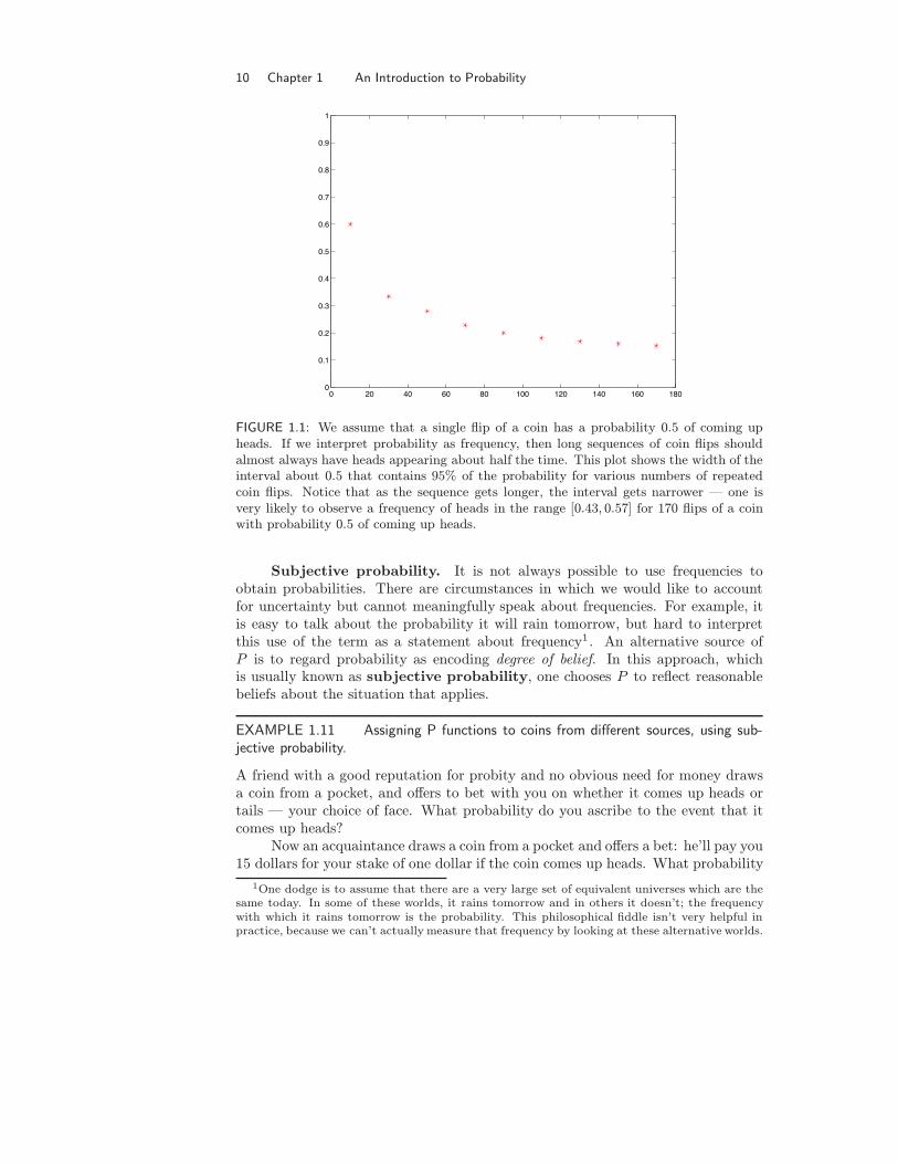
• and secondly, because the probability assigned to these long sequences canalso be interpreted as a frequency — essentially, this interpretation meansthat long sequences where the events occur with the “right” frequency occurfar more often than other such sequences (see figure 1.1).

All this means that, if we choose a P function for a coin flip — or some otherexperiment — on the basis of sufficiently good frequency data, then we are veryunlikely to see long sequences of coin flips — or repetitions of the experiment —that do not show this frequency.

This interpretation of probability as frequency is widespread, and common.One valuable advantage of the interpretation is that it simplifies estimating prob-abilities for some sorts of models. For example, given a coin, one could obtainP (heads) by flipping the coin many times and measuring the relative frequencywith which heads appear.


0 20 40 60 80 100 120 140 160 1800

0.1

0.2

0.3

0.4

0.5

0.6

0.7

0.8

0.9

1

FIGURE 1.1: We assume that a single flip of a coin has a probability 0.5 of coming upheads. If we interpret probability as frequency, then long sequences of coin flips shouldalmost always have heads appearing about half the time. This plot shows the width of theinterval about 0.5 that contains 95% of the probability for various numbers of repeatedcoin flips. Notice that as the sequence gets longer, the interval gets narrower — one isvery likely to observe a frequency of heads in the range [0.43, 0.57] for 170 flips of a coinwith probability 0.5 of coming up heads.

Subjective probability. It is not always possible to use frequencies toobtain probabilities. There are circumstances in which we would like to accountfor uncertainty but cannot meaningfully speak about frequencies. For example, itis easy to talk about the probability it will rain tomorrow, but hard to interpretthis use of the term as a statement about frequency1 . An alternative source ofP is to regard probability as encoding degree of belief. In this approach, whichis usually known as subjective probability, one chooses P to reflect reasonablebeliefs about the situation that applies.

EXAMPLE 1.11 Assigning P functions to coins from different sources, using sub-jective probability.

A friend with a good reputation for probity and no obvious need for money drawsa coin from a pocket, and offers to bet with you on whether it comes up heads ortails — your choice of face. What probability do you ascribe to the event that itcomes up heads?

Now an acquaintance draws a coin from a pocket and offers a bet: he’ll pay you15 dollars for your stake of one dollar if the coin comes up heads. What probability

1One dodge is to assume that there are a very large set of equivalent universes which are thesame today. In some of these worlds, it rains tomorrow and in others it doesn’t; the frequencywith which it rains tomorrow is the probability. This philosophical fiddle isn’t very helpful inpractice, because we can’t actually measure that frequency by looking at these alternative worlds.

Section 1.2 Probability in Continuous Spaces 11

do you ascribe to the event that it comes up heads?Finally you encounter someone in a bar who (it emerges) has a long history of

disreputable behaviour and an impressive conviction record. This person producesa coin from a pocket and offers a bet: you pay him 1000 dollars for his stake of onedollar if it lands on its edge and stands there. What probability do you ascribe tothe event that it lands on its edge and stands there?

You have to choose your answer for these cases — that’s why it’s subjective.You could lose a lot of money learning that the answer in the second case is goingto be pretty close to zero. Similarly, the answer in the third case is pretty close toone. There is a lot of popular and literary information about subjective probability.People who are thoughtless in there estimates of subjective probability offer a livingto those of sharp wits; John Bradshaw’s wonderful book “Fast Company” is afascinating account of this world. One version of the third case — that if you betwith a stranger that a card will not leap out of a pack and squirt cider in your ear,you will end up with a wet ear — is expounded in detail in Damon Runyon’s story“The Idyll of Miss Sarah Brown.”

Subjective probability must still satisfy the axioms of probability. It is simplya way of choosing free parameters in a probability model without reference tofrequency. The attractive feature of subjective probability is that it emphasizes thata choice of probability model is a modelling exercise — there are few circumstanceswhere the choice is canonical. One natural technique to adopt is to choose a functionP that yields good behaviour in practice; this strategy is pervasive through thefollowing chapters.

1.2 PROBABILITY IN CONTINUOUS SPACES

Much of the discussion above transfers quite easily to a continuous space, as longas we are careful about events. The difficulty is caused by the “size” of continuousspaces — there are an awful lot of numbers between 1.0 and 1.00000001, one for eachnumber between 1.0 and 2.0. For example, if we are observing noise — perhaps bymeasuring the voltage across the terminals of a warm resistor — the noise will veryseldom take the value 1 exactly. It is much more helpful to consider the probabilitythat the value is in the range 1 to 1 + δ, for δ a small step.

1.2.1 Event Structures for Continuous Spaces

This observation justifies using events that look like intervals or boxes for continuousspaces. Given a space D, our space of events will be a set F with the followingproperties:

• The empty set is in F and so is D.

• Closure under finite intersections: if Si is a finite collection of subsets, andeach Si ∈ F then ∩iSi ∈ F .

• Closure under finite unions: if Si is an finite collection of subsets, and eachSi ∈ F then ∪iSi ∈ F .

• Closure under complements: if S1 ∈ F then S1 = D − S1 ∈ F .


The basic axioms for P apply here too. For D the domain, and A and B events,we have:

• P (D) = 1

• P (∅) = 0

• for any A, 0 ≤ P (A) ≤ 1

• if A ⊂ B, then P (A) ≤ P (B)

• P (A ∪B) = P (A) + P (B)− P (A ∩B)

The concepts of conditional probability, independence and conditional indepen-dence apply in continuous spaces without modification. For example, the condi-tional probability of an event given another event can be defined by

P (A ∩B) = P (A|B)P (B)

and the conditional probability can be thought of as probability restricted to theset B. Events A and B are independent if and only if

P (A ∩B) = P (A)P (B)

and A and B are conditionally independent given C if and only if

P (A ∩B|C) = P (A|C)P (B|C)

Of course, to build a useful model we need to be more specific about what theevents should be.

1.2.2 Representing P-functions

One difficulty in building probability models on continuous spaces is expressing thefunction P in a useful way — it is clearly no longer possible to write down thespace of events and give a value of P for each event. We will deal only with Rn,with subsets of this space, or with multiple copies of this space.

The Real Line.The set of events for the real line is far too big to write down. All events look

like unions of a basic collection of sets. This basic collection consists of:

• individual points (i.e a);

• open intervals (i.e. (a, b));

• half-open intervals (i.e. (a, b] or [a, b));

• and closed intervals (i.e. [a, b]).

All of these could extend to infinity. The function P can be represented by afunction F with the following properties:

Section 1.2 Probability in Continuous Spaces 13

• F (−∞) = 0

• F (∞) = 1

• F (x) is monotonically increasing.

and we interpret F (x) as P ((−∞, x]). The function F is referred to as the cu-mulative distribution function. The value of P for all the basic sets de-scribed can be extracted from F , with appropriate attention to limits; for example,P ((a, b]) = F (b)− F (a) and P (a) = limε←0+(F (a)− F (a− ε)). Notice that if F iscontinuous, P (a) = 0.

Higher Dimensional Spaces.In Rn, events are unions of elements of a basic collection of sets, too. This

basic collection consists of a product of n elements from the basic collection for thereal line. A cumulative distribution function can be defined in this case, too. It isgiven by a function F with the property that P ({x1 ≤ u1, x2 ≤ u2, . . . xn ≤ un}) =F (u). This function is constrained by other properties, too. However, cumulativedistribution functions are a somewhat unwieldy way to specify probability.

1.2.3 Representing P-functions with Probability Density Functions

For the examples we will deal with in continuous spaces, the usual way to specifyP is to provide a function p such that

P (event) =

∫event

p(u)du

This function is referred to as a probability density function.Not every probability model admits a density function, but all our cases will.

Note that a density function cannot have a negative value, but that its value couldbe larger than one. In all cases, probability density functions integrate to one, i.e.

P (D) =

∫D

p(u)du = 1

and any non-negative function with this property is a probability density function.The value of the probability density function at a point represents the probabilityof the event that consists of an infinitesimal neighbourhood at that value, i.e.:

p(u1)du = P ({u ∈ [u1, u1 + du]})

Notice that this means that (unless we are willing to be rather open minded aboutwhat constitutes a function), for a probability model on a continuous space that canbe represented using a probability density, the probability of an event that consistsof a finite union of points must be zero. For the examples we will deal with, thisdoesn’t create any issues. In fact, it is intuitive, in the sense that we don’t expectto be able to observe the event that, say, a noise voltage has value 1; instead, wecan observe the event that it lies in some tiny interval — defined by the accuracyof our measuring equipment — about 1.

Conditional probability, independence and conditional independence are ideasthat can be translated into properties of probability density functions. In their mostuseful form, they are properties of random variables.


1.3 RANDOM VARIABLES

Assume that we have a probability model on either a discrete or a continuousdomain, {D,F , P }. Now let us consider a function of the outcome of an experiment.The values that this function takes on the different elements of D form a new set,which we shall call D′. There is a structure, with the same formal properties as Fon D′ defined by the values that this function takes on different elements of F —call this structure F ′.

This function is known as a random variable. We can talk about the proba-bility that a random variable takes a particular set of values, because the probabilitystructure carries over. In particular, assume that we have a random variable ξ. IfA′ ∈ F ′, there is some A ∈ F such that A′ = ξ(A). This means that

P ({ξ ∈ A′}) = P (A)

EXAMPLE 1.12 Assorted examples of random variables

The simplest random variable is given by the identity function — this means thatD′ is the same as D, and F ′ is the same as F . For example, the outcome of a coinflip is a random variable.

Now gamble on the outcome of a coin flip: if it comes up heads, you get adollar, and if it comes up tails, you pay a dollar. Your income from this gamble isa random variable. In particular, D′ = {1,−1} and F ′ = {∅, D′, {1}, {−1}}.

Now gamble on the outcome of two coin flips: if both coins come up the same,you get a dollar, and if they come up different, you pay a dollar. Your income fromthis gamble is a random variable. Again, D′ = {1,−1} and F ′ = {∅, D′, {1}, {−1}}.In this case, D′ is not the same as D and F ′ is not the same as F ; however, wecan still speak about the probability of getting a dollar — which is the same asP ({hh, tt}).

Density functions are very useful for specifying the probability model for thevalue of a random variable. However, they do result in quite curious notations(probability is a topic that seems to encourage creative use of notation). It iscommon to write the density function for a random variable as p. Thus, the dis-tribution for λ would be written as p(λ) — in this case, the name of the variabletells you what function is being referred to, rather than the name of the function,which is always p. Some authors resist this convention, but its use is pretty muchuniversal in the vision literature, which is why we adopt it. For similar reasons,we write the probability function for a set of events as P , so that the probabilityof an event P (event) (despite the fact that different sets of events may have verydifferent probability functions).

1.3.1 Conditional Probability and Independence

Conditional probability is a very useful idea for random variables. Assume wehave two random variables, m and n— (for example, the value I read from my raingauge asm and the value I read on the neighbour’s as n). Generally, the probability

Section 1.3 Random Variables 15

density function is a function of both variables, p(m, n). Now

p(m1, n1)dmdn = P ({m ∈ [m1 , m1 + dm]} and {n ∈ [n1, n1 + dm]})

= P ({m ∈ [m1 , m1 + dm]} | {n ∈ [n1, n1 + dm]})P ({n ∈ [n1, n1 + dm]})

We can define a conditional probability density from this by

p(m1, n1)dmdn = P ({m ∈ [m1 , m1 + dm]} | {n ∈ [n1, n1 + dm]})P ({n ∈ [n1, n1 + dm]})

= (p(m1 |n1)dm)(p(n1)dn)

Note that this conditional probability density has the expected property, that

p(m|n) =p(m, n)

p(n)

Independence and conditional independence carry over to random variables andprobability densities without fuss.

EXAMPLE 1.13 Independence in random variables associated with two coins.

We now consider the probability that each of two different coins comes up heads.In this case, we have two random variables, being the probability that the firstcoin comes up heads and the probability that the second coin comes up heads (it’squite important to understand why these are random variables — if you’re not sure,look back at the definition). We shall write these random variables as p1 and p2.Now the density function for these random variables is p(p1, p2). Let us assumethat there is no dependency between these coins, so we should be able to writep(p1, p2) = p(p1)p(p2). Notice that the notation is particularly confusing here; theintended meaning is that p(p1, p2) factors, but that the factors are not necessarilyequal. In this case, a further reasonable modelling step is to assume that p(p1) isthe same function as p(p2) (perhaps they came from the same minting machine).

1.3.2 Expectations

The expected value or expectation of a random variable (or of some functionof the random variable) is obtained by multiplying each value by its probabilityand summing the results — or, in the case of a continuous random variable, bymultiplying by the probability density function and integrating. The operation isknown as taking an expectation. For a discrete random variable, x, taking theexpectation of x yields:

E[x] =∑

i∈values

xip(xi)

For a continuous random variable, the process yields

E[x] =

∫D

xp(x)dx


often referred to as the average, or the mean in polite circles. One model for anexpectation is to consider the random variable as a payoff, and regard the expec-tation as the average reward, per bet, for an infinite number of repeated bets. Theexpectation of a general function g(x) of a random variable x is written as E[g(x)].

The variance of a random variable x is

var(x) = E[x2 − (E(x))2]

This expectation measures the average deviance from the mean. The variance ofa random variable gives quite a strong indication of how common it is to see avalue that is significantly different from the mean value. In particular, we have thefollowing useful fact:

P ({|x− E[x] |≥ ε}) ≤var(x)

ε2

The standard deviation is obtained from the variance:

sd(x) =√var(x) =

√E[x2 − (E[x])2]

For a vector of random variables, the covariance is

cov(x) = E[xxt − (E[x]E[x]t)]

This matrix (look carefully at the transpose) is symmetric. Diagonal entries arethe variance of components of x, and must be non-negative. Off-diagonal elementsmeasure the extent to which two variables co-vary. For independent variables, thecovariance must be zero. For two random variables that generally have differentsigns, the covariance can be negative.

EXAMPLE 1.14 The expected value of gambling on a coin flip.

You and an acquaintance decide to bet on the outcome of a coin flip. You willreceive a dollar from your acquaintance if the coin comes up heads, and pay one ifit comes up tails. The coin is symmetric.

This means the expected value of the payoff is

1P (heads)− 1P (tails) = 0

The variance of the payoff is one, as is the standard deviation.Now consider the probability of obtaining 10 dollars in 10 coin flips, with a

fair coin. Our random variable x is the income in 10 coin flips. Equation 1.3.2 yieldsP ({|x |≥ 10}) ≤ 1

100 , which is a generous upper bound — the actual probability isof the order of one in a thousand.

Expectations of functions of random variables are extremely useful. The no-tation for expectations can be a bit confusing, because it is common to omit thedensity with respect to which the expectation is being taken, which is usually ob-vious from the context. For example, E[x2] is interpreted as∫

D

x2p(x)dx

Section 1.3 Random Variables 17

1.3.3 Joint Distributions and Marginalization

Assume we have a model describing the behaviour of a collection of random vari-ables. We will proceed on the assumption that they are discrete, but (as shouldbe clear by now) the discussion will work for continuous variables if summing isreplaced by integration. One way to specify this model is to give the probabilitydistribution for all variables, known in jargon as the joint probability distribu-tion function— for concreteness, write this as P (x1, x2, . . .xn). If the probabilitydistribution is represented by its density function, the density function is usuallyreferred to as the joint probability density function. Both terms are oftenabbreviated as “joint.”

EXAMPLE 1.15 Marginalising out parameters for two different types of coin.

Let us assume we have a coin which could be from one of two types; the first typeof coin is evenly balanced; the other is wildly unbalanced. We flip our coin somenumber of times, observe the results, and should like to know what type of coin wehave. Assume that we flip the coin once. The set of outcomes is

D = {(heads, I), (heads, II), (tails, I), (tails, II)}

An appropriate event space is:

∅, D,{(heads, I)}, {(heads, II)},{(tails, I)}, {(tails, II)},

{(heads, I), (heads, II)} , {(tails, I), (tails, II),} ,{(tails, I), (heads, I)} , {(tails, II), (heads, II)} ,

{(heads, II), (tails, I), (tails, II)}, {(heads, I), (tails, I), (tails, II)}{(heads, I), (heads, II), (tails, II)} {(heads, I), (heads, II), (tails, I)}

In this case, assume that we know P (face, type), for each face and type. Now, forexample, the event that the coin shows heads (whatever the type) is representedby the set

{(heads, I), (heads, II)}

We can compute the probability that the coin shows heads (whatever the type) asfollows

P ({(heads, I), (heads, II)}) = P ((heads, I) ∪ (heads, II))

= P ({(heads, I)}) + P ({(heads, II)})

We can compute the probability that the coin is of type I, etc. with similar easeusing the same line of reasoning, which applies quite generally.

As we have already seen, the value of P for some elements of the event spacecan be determined from the value of P for other elements. This means that if weknow

P ({x1 = a, x2 = b, . . . xn = n})

for each possible value of a, b, . . . , n, then we should know P for a variety of otherevents. For example, it might be useful to know P ({x1 = a}). If we can formP ({x2 = b, . . . xn = n}) from P ({x1 = a, x2 = b, . . . xn = n}), then we can obtain


any other (smaller) set of values too by the same process. You should now look atexample 15, which illustrates how the process works using the event structure fora simple case.

In fact, the event structure is getting unwieldy as a notation. It is quitecommon to use a rather sketchy notation to indicate the appropriate event. Forexample 15, we would write

P ({(heads, I), (heads, II)}) = P (heads)

We would like to form P ({x2 = b, . . . xn = n}) from P ({x1 = a, x2 = b, . . . xn = n}).By using the argument about event structures in example 15, we obtain

P (x2 = b, . . .xn = n) =∑

v∈values of x1

P (x1 = v, x2 = b, . . .xn = n)

which we could write as

P (x2, . . . xn) =∑

values of x1

P (x1, x2, . . .xn)

This operation is referred to as marginalisation. marginalisationA similar argument applies to probability density functions, but the operation

is now integration. Given a probability density function p(x1, x2, . . . , xn), we obtain

p(x2, . . . xn) =

∫D

p(x1, x2, . . . xn)dx1

marginalisation

1.4 STANDARD DISTRIBUTIONS AND DENSITIES

There are a variety of standard distributions that arise regularly in practice. Ref-erences such as [Patel et al., 1976; Evans et al., 2000] give large numbers; we willdiscuss only the most important cases.

The uniform distribution has the same value at each point on the domain.This distribution is often used to express an unwillingness to make a choice or alack of information. On a continuous space, the uniform distribution has a densityfunction that has the same value at each point. Notice that a uniform density onan infinite continuous domain isn’t meaningful, because it could not be scaled tointegrate to one. In practice, one can often avoid this point, either by pretendingthat the value is a very small constant and arranging for it to cancel, or using anormal distribution (described below) with a really big covariance, such that itsvalue doesn’t change much over the region of interest.

The binomial distribution applies to situations where one has independentidentically distributed samples from a distribution with two values. For example,consider drawing n balls from an urn containing equal numbers of black and whiteballs. Each time a ball is drawn, its colour is recorded and it is replaced, so thatthe probability of getting a white ball — which we denote p — is the same for eachdraw. The binomial distribution gives the probability of getting k white balls(

nk

)pk(1− p)n−k

Section 1.4 Standard Distributions and Densities 19

The mean of this distribution is np and the variance is np(1− p).

The Poisson distribution applies to spatial models that have uniformityproperties. Assume that points are placed on the real line randomly in such a waythat the expected number of points in an interval is proportional to the length ofthe interval. The number of points in a unit interval will have a Poisson distributionwhere

P ({N = x}) =λxe−x

x!

(where x = 0, 1, 2 . . . and λ > 0 is the constant of proportionality). The mean ofthis distribution is λ and the variance is λ

1.4.1 The Normal Distribution

The probability density function for the normal distribution for a single randomvariable x is

p(x;µ, σ) =1

√2πσ

exp−

{(x− µ)2

2σ2

}

The mean of this distribution is µ and the standard deviation is σ. This distributionis widely called a Gaussian distribution in the vision community.

The multivariate normal distribution for d-dimensional vectors x hasprobability density function

p(x;µ,Σ) =1

(2π)d2 det(Σ)1/2

exp−

{(x− µ)TΣ−1(x−µ)

2

}

The mean of this distribution is µ and the covariance is Σ. Again, this distributionis widely called a Gaussian distribution in the vision community.

The normal distribution is extremely important in practice, for several rea-sons:

• The sum of a large number of random variables is normally distributed, prettymuch whatever the distribution of the individual random variables. This factis known as the central limit theorem. It is often cited as a reason tomodel a collection of random effects with a single normal model.

• Many computations that are prohibitively hard for any other case are easyfor the normal distribution.

• In practice, the normal distribution appears to give a fair model of some kindsof noise.

• Many probability density functions have a single peak and then die off; amodel for such distributions can be obtained by taking a Taylor series of thelog of the density at the peak. The resulting model is a normal distribution(which is often quite a good model).


1.5 PROBABILISTIC INFERENCE

Very often, we have a sequence of observations produced by some process whosemechanics we understand, but which has some underlying parameters that we donot know. The problem is to make useful statements about these parameters. Forexample, we might observe the intensities in an image, which are produced by theinteraction of light and surfaces by principles we understand; what we don’t know— and would like to know — are such matters as the shape of the surface, thereflectance of the surface, the intensity of the illuminant, etc. Obtaining somerepresentation of the parameters from the data set is known as inference. Thereis no canonical inference scheme; instead, we need to choose some principle thatidentifies the most desirable set of parameters.

1.5.1 The Maximum Likelihood Principle

A general inference strategy known as maximum likelihood inference, can bedescribed as

Choose the world parameters that maximise the probability of the mea-surement observed

In the general case, we are choosing

argmaxP (measurements|parameters)

(where the maximum is only over the world parameters because the measurementsare known, and argmax means “the argument that maximises”). In many prob-lems, it is quite easy to specify the measurements that will result from a particularsetting of model parameters — this means that P (measurements|parameters), oftenreferred to as the likelihood, is easy to obtain. This can make maximum likelihoodestimation attractive.

EXAMPLE 1.16 Maximum likelihood inference on the type of a coin from its be-haviour.

We return to example 15. Now assume that we know some conditional probabilities.In particular, the unbiased coin has P (heads|I) = P (tails|I) = 0.5, and the biasedcoin has P (tails|II) = 0.2 and P (heads|II) = 0.8.

We observe a series of flips of a single coin, and wish to know what type of coinwe are dealing with. One strategy for choosing the type of coin represented by ourevidence is to choose either I or II, depending on whether P (flips observed|I) >P (flips observed|II). For example, if we observe four heads and one tail insequence, then P (hhhht|II) = (0.8)40.2 = 0.08192 and P (hhhht|I) = 0.03125, andwe choose type II.

Maximum likelihood is often an attractive strategy, because it can admit quitesimple computation. A classical application of maximum likelihood estimationinvolves estimating the parameters of a normal distribution from a set of samplesof that distribution (example 17).

Section 1.5 Probabilistic Inference 21

EXAMPLE 1.17 Estimating the parameters of a normal distribution from a seriesof independent samples from that distribution.

Assume that we have a set of n samples — the i’th of which is xi — that are knownto be independent and to have been drawn from the same normal distribution. Thelikelihood of our sample is

P (sample|µ, σ) = L(x1, . . . xn;µ, σ)

=∏i

p(xi;µ, σ) =∏i

1√2πσ

exp

(−(xi − µ)2

2σ2

)

Working with the log of the likelihood will remove the exponential, and not changethe position of the maximum. For the log-likelihood, we have

Q(x1, . . . xn;µ, σ) = −∑i

(xi − µ)2

2σ2− n(

1

2log 2 +

1

2log π + log σ)

and we want the maximum with respect to µ and σ. This must occur when thederivatives are zero, so we have

∂Q

∂µ= 2∑i

(xi − µ)

2σ2= 0

and a little shuffling of expressions shows that this maximum occurs at

µ =

∑i xi

n

Similarly∂Q

∂σ=

∑i(xi − µ)

2

σ3−n

σ= 0

and this maximum occurs at

σ =

√∑i(xi − µ)

2

n

Note that this estimate of σ is biased, in that its expected value is σ(n/(n − 1))and it is more usual to use (1/(n− 1))

√∑i(xi − µ)

2 as an estimate.

1.5.2 Priors, Posteriors and Bayes’ rule

In example 16, our maximum likelihood estimate incorporates no information aboutP (I) or P (II) — which can be interpreted as how often coins of type I or type IIare handed out, or as our subjective degree of belief that we have a coin of type Ior of type II before we flipped the coin. This is unfortunate, to say the least; forexample, if coins of type II are rare, we would want to see an awful lot of headsbefore it would make sense to infer that our coin is of this type. Some quite simplealgebra suggests a solution.


Recall that P (A,B) = P (A|B)P (B). This simple observation gives rise to aninnocuous looking identity for reversing the order in a conditional probability:

P (B|A) =P (A|B)P (B)

P (A)

This is widely referred to as Bayes’ theorem or Bayes’ rule.Now the interesting property of Bayes’ rule is that it tells us which choice

of parameters is most probable, given our model and our prior beliefs. RewritingBayes’ rule gives

P (parameters|data) =P (data|parameters)P (parameters)

P (data)

The term P (parameters) is referred to as the prior (it describes our knowledge ofthe world before measurements have been taken). The term P (parameters|data) isusually referred to as the posterior (it describes the probability of various modelsafter measurements have been taken). P (data) can be computed by marginalisation(which requires computing a high dimensional integral, often a nasty business) orfor some problems can be ignored. As we shall see in following sections, attemptingto use Bayes’ rule can result in difficult computations — that integral being one —because posterior distributions often take quite unwieldy forms.

1.5.3 Bayesian Inference

The Bayesian philosophy is that

all information about the world is captured by the posterior.

The first reason to accept this view is that the posterior is a principled combinationof prior information about the world and a model of the process by which measure-ments are generated — i.e. there is no information missing from the posterior, andthe information that is there, is combined in a proper manner. The second reasonis that the approach appears to produce very good results. The great difficulty isthat computing with posteriors can be very difficult — we will encounter variousmechanisms for computing with posteriors in following sections.

For example, we could use the study of physics in the last few chapters to getexpressions relating pixel values to the position and intensity of light sources, thereflectance and orientation of surfaces, etc. Similarly, we are likely to have somebeliefs about the parameters that have nothing to do with the particular values ofthe measurements that we observe. We know that albedos are never outside therange [0, 1]; we expect that illuminantswith extremely high exitance are uncommon;and we expect that no particular surface orientation is more common than anyother. This means that we can usually cobble up a reasonable choice of prior.

MAP Inference. An alternative to maximum likelihood inference is to infera state of the world that maximises the posterior:

Choose the world parameters that maximise the conditional probabilityof the parameters, conditioned on the measurements taking the observedvalues


This approach is known as maximum a posteriori (or MAP) reasoning.

EXAMPLE 1.18 Determining the type of a coin using MAP inference.

Assume that we have three flips of the coin of example 16, and would like todetermine whether it has type I or type II. We know that the mint has 3 machinesthat produce type I coins and 1 machine that produces type II coins, and there isno reason to believe that these machines run at different rates. We therefore assignP (I) = 0.75 and P (II) = 0.25. Now we observe three heads, in three consecutiveflips. The value of the posterior for type I is:

P (I|hhh) =P (hhh|I)P (I)

P (hhh)

=P (h|I)3P (I)

P (hhh, I) + P (hhh, II)

=P (h|I)3P (I)

P (hhh|I)P (I) + P (hhh|II)P (II)

=0.530.75

0.530.75 + 0.830.25

= 0.422773

By a similar argument, the value of the posterior for type II is 0.577227. An MAPinference procedure would conclude the coin is of type II.

The denominator in the expression for the posterior can be quite difficult tocompute, because it requires a sum over what is potentially a very large number ofelements (imagine what would happen if there were many different types of coin).However, knowing this term is not crucial if we wish to isolate the element with themaximum value of the posterior, because it is a constant. Of course, if there area very large number of events in the discrete space, finding the world parametersthat maximise the posterior can be quite tricky.

The Posterior as an Inference.

EXAMPLE 1.19 Determining the probability a coin comes up heads from the out-come of a sequence of flips.

Assume we have a coin which comes from a mint which has a continuous controlparameter, λ, which lies in the range [0, 1]. This parameter gives the probabilitythat the coin comes up heads, so P (heads|λ) = λ. We know no reason to preferany one value of λ to any other, so as a prior probability distribution for λ we usethe uniform distribution so p(λ) = 1.

Assume we flip the coin twice, and observe heads twice; what do we knowabout λ? All our knowledge is captured by the posterior, which is

P (λ ∈ [x, x+ dx]|hh)

dx


we shall write this expression as p(λ|hh). We have

p(λ|hh) =p(hh|λ)p(λ)

p(hh)

=p(hh|λ)p(λ)∫ 1

0p(hh|λ)p(λ)dλ

=λ2p(λ)∫ 1

0 p(hh|λ)p(λ)dλ

= 3λ2

It is fairly easy to see that if we flip the coin n times, and observe k heads and n−ktails, we have

p(λ|k heads and n− k tails) ∝ λk(1− λ)n−k

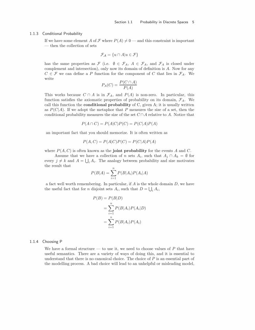
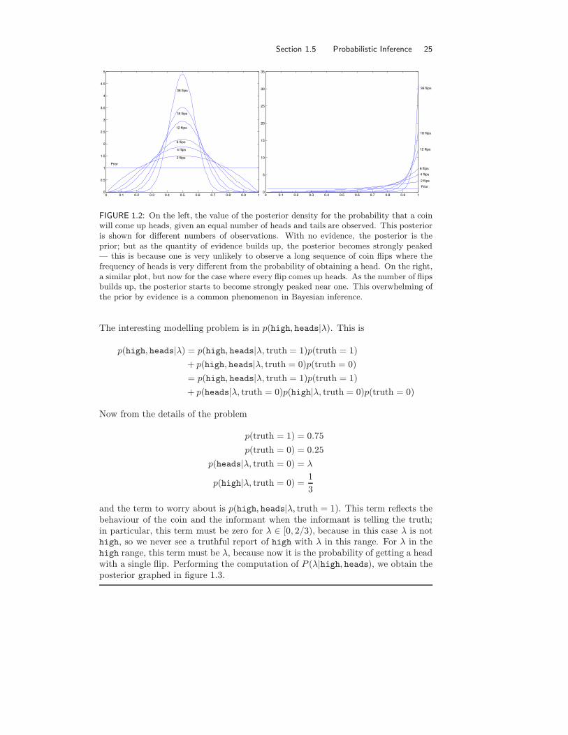
We have argued that choosing parameters that maximise the posterior is auseful inference mechanism. But, as figure 1.2 indicates, the posterior is good forother uses as well. This figure plots the posterior distribution on the probabilitythat a coin comes up heads, given the result of some number of flips. In thefigure, the posterior distributions indicate not only the single “best” value for theprobability that a coin comes up heads, but also the extent of the uncertainty inthat value. For example, inferring a value of this probability after two coin flipsleads to a value that is not particularly reliable — the posterior is a rather flatfunction, and there are many different values of the probability with about thesame value of the posterior. Possessing this information allows us to compare thisevidence with other sources of evidence about the coin.

Bayesian inference is a framework within which it is particularly easy to com-bine various types of evidence, both discrete and continuous. It is often quite easyto set up the sums.

EXAMPLE 1.20 Determining the type of a coin from a sequence of flips, incorpo-rating information from an occasionally untruthful informant.

We use the basic setup of example 19. Assume you have a contact at the coinfactory, who will provide a single estimate of λ. Your contact has poor discrimi-nation, and can tell you only whether λ is low, medium or high (i.e in the range[0, 1/3], (1/3, 2/3) or [2/3, 1]). You expect that a quarter of the time your contact,not being habitually truthful, will simply guess rather than checking how the coinmachine is set. What do you know about λ after a single coin flip, which comes upheads, if your contact says high? We need

p(λ|high, heads) =p(high, heads|λ)p(λ)

p(high, heads)

∝ p(high, heads|λ)p(λ)


0 0.1 0.2 0.3 0.4 0.5 0.6 0.7 0.8 0.9 10

0.5

1

1.5

2

2.5

3

3.5

4

4.5

5

Prior

2 flips

4 flips

6 flips

12 flips

18 flips

36 flips

0 0.1 0.2 0.3 0.4 0.5 0.6 0.7 0.8 0.9 10

5

10

15

20

25

30

35

Prior

2 flips

4 flips

6 flips

12 flips

18 flips

36 flips

FIGURE 1.2: On the left, the value of the posterior density for the probability that a coinwill come up heads, given an equal number of heads and tails are observed. This posterioris shown for different numbers of observations. With no evidence, the posterior is theprior; but as the quantity of evidence builds up, the posterior becomes strongly peaked— this is because one is very unlikely to observe a long sequence of coin flips where thefrequency of heads is very different from the probability of obtaining a head. On the right,a similar plot, but now for the case where every flip comes up heads. As the number of flipsbuilds up, the posterior starts to become strongly peaked near one. This overwhelming ofthe prior by evidence is a common phenomenon in Bayesian inference.

The interesting modelling problem is in p(high, heads|λ). This is

p(high, heads|λ) = p(high, heads|λ, truth = 1)p(truth = 1)

+ p(high, heads|λ, truth = 0)p(truth = 0)

= p(high, heads|λ, truth = 1)p(truth = 1)

+ p(heads|λ, truth = 0)p(high|λ, truth = 0)p(truth = 0)

Now from the details of the problem

p(truth = 1) = 0.75

p(truth = 0) = 0.25

p(heads|λ, truth = 0) = λ

p(high|λ, truth = 0) =1

3

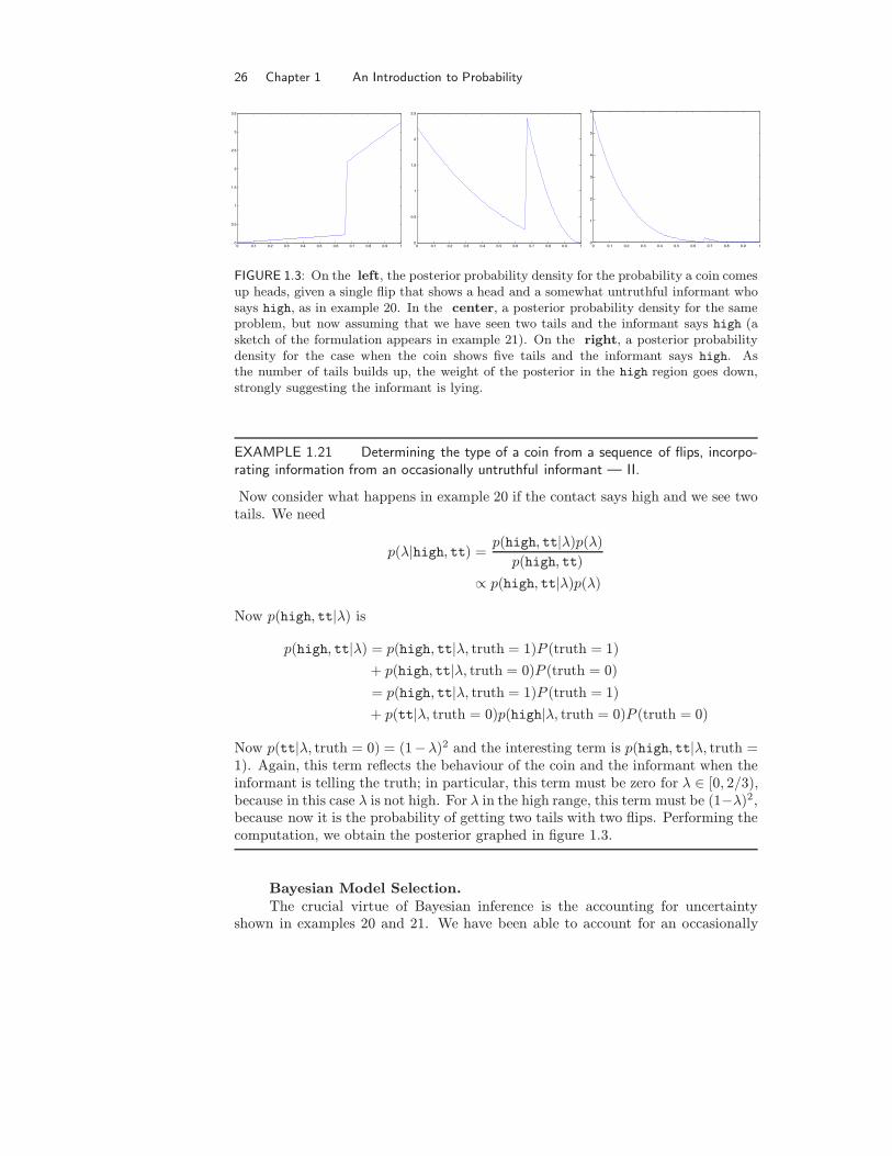
and the term to worry about is p(high, heads|λ, truth = 1). This term reflects thebehaviour of the coin and the informant when the informant is telling the truth;in particular, this term must be zero for λ ∈ [0, 2/3), because in this case λ is nothigh, so we never see a truthful report of high with λ in this range. For λ in thehigh range, this term must be λ, because now it is the probability of getting a headwith a single flip. Performing the computation of P (λ|high, heads), we obtain theposterior graphed in figure 1.3.


0 0.1 0.2 0.3 0.4 0.5 0.6 0.7 0.8 0.9 10

0.5

1

1.5

2

2.5

3

3.5

0 0.1 0.2 0.3 0.4 0.5 0.6 0.7 0.8 0.9 10

0.5

1

1.5

2

2.5

0 0.1 0.2 0.3 0.4 0.5 0.6 0.7 0.8 0.9 10

1

2

3

4

5

6

FIGURE 1.3: On the left, the posterior probability density for the probability a coin comesup heads, given a single flip that shows a head and a somewhat untruthful informant whosays high, as in example 20. In the center, a posterior probability density for the sameproblem, but now assuming that we have seen two tails and the informant says high (asketch of the formulation appears in example 21). On the right, a posterior probabilitydensity for the case when the coin shows five tails and the informant says high. Asthe number of tails builds up, the weight of the posterior in the high region goes down,strongly suggesting the informant is lying.

EXAMPLE 1.21 Determining the type of a coin from a sequence of flips, incorpo-rating information from an occasionally untruthful informant — II.

Now consider what happens in example 20 if the contact says high and we see twotails. We need

p(λ|high, tt) =p(high, tt|λ)p(λ)

p(high, tt)

∝ p(high, tt|λ)p(λ)

Now p(high, tt|λ) is

p(high, tt|λ) = p(high, tt|λ, truth = 1)P (truth = 1)

+ p(high, tt|λ, truth = 0)P (truth = 0)

= p(high, tt|λ, truth = 1)P (truth = 1)

+ p(tt|λ, truth = 0)p(high|λ, truth = 0)P (truth = 0)

Now p(tt|λ, truth = 0) = (1−λ)2 and the interesting term is p(high, tt|λ, truth =1). Again, this term reflects the behaviour of the coin and the informant when theinformant is telling the truth; in particular, this term must be zero for λ ∈ [0, 2/3),because in this case λ is not high. For λ in the high range, this term must be (1−λ)2,because now it is the probability of getting two tails with two flips. Performing thecomputation, we obtain the posterior graphed in figure 1.3.

Bayesian Model Selection.The crucial virtue of Bayesian inference is the accounting for uncertainty

shown in examples 20 and 21. We have been able to account for an occasionally


untruthful informant and a random measurement; when there was relatively littlecontradictory evidence from the coin’s behaviour, our process placed substantialweight on the informant’s testimony, but when the coin disagreed, the informantwas discounted. This behaviour is highly attractive, because we are able to combineuncertain sources of information with confidence.

EXAMPLE 1.22 Is the informant lying?

We now need to know whether our informant lied to us. Assume we see a singlehead and an informant saying high, again. The relevant posterior is:

P (truth=0|head, high) =P (head, high|truth=0)P (truth=0)

P (head, high)

=

∫P (λ, head, high|truth=0)P (truth=0)dλ

P (head, high)

=

∫P (head, high|λ, truth=0)P (λ)P (truth=0)dλ

P (head, high)

=1

1 +

∫P(head,high|λ,truth=1)P(λ)dλP(truth=1)∫P(head,high|λ,truth=0)P(λ)dλP(truth=0)

Example 22 shows how to tell whether the informant of examples 20 and 21is telling the truth or not, given the observations. A useful way to think aboutthis example is to regard it as comparing two models (as opposed to the value ofa binary parameter within one model). One model has a lying informant, and theother has a truthful informant. The posteriors computed in this example comparehow well different models explain a given data set, given a prior on the models.This is a very general problem — usually called model selection — with a widevariety of applications in vision:

• Recognition: Assume we have a region in an image, and an hypothesis thatan object might be present in that region at a particular position and orienta-tion (the hypothesis will have been obtained using methods from chapter ??,which aren’t immediately relevant). Is there an object there or not? A prin-cipled answer involves computing the posterior over two models — that thedata was obtained from noise, or from the presence of an object.

• Are these the same? Assume we have a set of pictures of surfaces we wantto compare. For example, we might want to know if they are the same colour,which would be difficult to answer directly if we didn’t know the illuminant.A principled answer involves computing the posterior over two models — thatthe data was obtained from one surface, or from two (or more).

• What camera was used? Assume we have a sequence of pictures of aworld. With a certain amount of work, it is usually possible to infer a greatdeal of information about the shape of the objects from such a sequence (e.g.


chapters ??, ?? and ??). The algorithms involved differ quite sharply, de-pending on the camera model adopted (i.e. perspective, orthographic, etc.).Furthermore, adopting the wrong camera model tends to lead to poor infer-ences. Determining the right camera model to use is quite clearly a modelselection problem.

• How many segments are there? We would like to break an image intocoherent components, each of which is generated by a probabilistic model.How many components should there be? (section ??).

The solution is so absurdly simple in principle (in practice, the computations canbe quite nasty) that it is easy to expect something more complex, and miss it. Wewill write out Bayes’ rule specialised to this case to avoid this:

P (model|data) =P (data|model)

P (data)

=

∫P (data|model, parameters)P (parameters)d{parameters}

P (data)

∝

∫P (data|model, parameters)P (parameters)d{parameters}

which is exactly the form used in the example. Notice that we are engagingin Bayesian inference here, too, and so can report the MAP solution or reportthe whole posterior. The latter can be quite helpful when it is difficult to dis-tinguish between models. For example, in the case of the dodgy informant, ifP (truth=0|data) = 0.5001, it may be undesirable to conclude the informant is ly-ing — or at least, to take drastic action based on this conclusion. The integral ispotentially rather nasty, which means that the method can be quite difficult to usein practice. Useful references include [Gelman et al., 1995; Carlin and Louis, 1996;Gamerman, 1997; Newman and Barkema, 1998; Evans and Swartz, 2000].

1.5.4 Open Issues

In the rest of the book, we will have regular encounters with practical aspects ofthe Bayesian philosphy. Firstly, although the posterior encapsulates all informationavailable about the world, we very often need to make discrete decisions — shouldwe shoot it or not? Typically, this decision making process requires some accountingfor the cost of false positives and false negatives.

Secondly, how do we build models? There are three basic sources of likelihoodfunctions and priors:

• Judicious design: it is possible to come up with models that are too hard tohandle computationally. Generally, models on very high-dimensional domainsare difficult to deal with, particularly if there is a great deal of interdependencebetween variables. For some models, quite good inference algorithms areknown. The underlying principle of this approach is to exploit simplificationsdue to independence and conditional independence.

• Physics: particularly in low-level vision problems, likelihood models followquite simply from physics. It is hard to give a set of design rules for this


strategy. It has been used with some success on occasion (see, for exam-ple, [Forsyth, 1999]).

• Learning: a poor choice of model results in poor performance, and a goodchoice of model results in good performance. We can use this observation totune the structure of models if we have a sufficient set of data. We describeaspects of this strategy in chapter ?? and in chapter ??.

Finally, the examples above suggest that posteriors can have a nasty functionalform. This intuition is correct, and there is a body of technique that can help handleugly posteriors which we explore as and when we need it (see also [Gelman et al.,1995; Carlin and Louis, 1996; Gamerman, 1997; Newman and Barkema, 1998]).


1.6 NOTES

Our discussion of probability is pretty much straight down the line. We havediscussed the subject in terms of σ-algebras (implicitly!) because that is the rightway to think about it. It is important to keep in mind that the foundations ofprobability are difficult, and that it takes considerable sophistication to appreciatepurely axiomatic probability. Very little real progress appears to have come fromasking “what does probability mean?”; instead, the right question is what it cando. The reason probabilistic inference techniques lie at the core of any solutionto serious vision problems is that probability is a good book-keeping technique forkeeping track of uncertainty.

Inference is hard, however. The great difficulty in applying probability is, inour opinion, arriving at a model that is both sufficiently accurate and sufficientlycompact to allow useful inference. This isn’t at all easy. A naive Bayesian viewof vision — write out a posterior using the physics of illumination and reflection,guess some reasonable priors, and then study the posterior — very quickly fallsapart. In terms of what representation should this posterior be written? andhow can we extract information from the posterior? These questions are excitingresearch topics. A number of advanced inference techniques appear in the visionliterature, including expectation maximisation (which we shall see in chapter ??; seealso [Wang and Adelson, 1993; Wang and Adelson, 1994; Adelson and Weiss, 1995;Adelson and Weiss, 1996; Dellaert et al., 2000]); sampling methods (for imagereconstruction [Geman and Geman, 1984]; for recognition [Ioffe and Forsyth, 1999;Zhu et al., 2000]; for structure from motion [Forsyth et al., 1999; Dellaert et al.,2000]; and for texture synthesis [Zhu et al., 1998]); dynamic programming (which weshall see in chapter ??; see also [Belhumeur and Mumford, 1992; Papademetris andBelhumeur, 1996; Ioffe and Forsyth, 1999; Felzenszwalb and Huttenlocher, 2000]);independent components analysis (for separating lighting and reflections [Farid andAdelson, 1999]); and various inference algorithms for Bayes nets (e.g. [Binford et al.,1989; Mann and Binford, 1992; Buxton and Gong, 1995; Kumar and Desai, 1996;Krebs et al., 1998]).

The examples in this chapter are all pretty simple, so as to expose the line ofreasoning required. We do some hard examples below. Building and handling com-plex examples is still very much a research topic; however, probabilistic reasoningof one form or another is now pervasive in vision, which is why it’s worth studying.

PROBLEMS

1.1. The event structure of section 1.1 did not explicitly include unions. Why does thetext say that unions are here?

1.2. In example 1, if P (heads) = p, what is P (tails)?

1.3. In example 10 show that if P (hh) = p2 then P ({ht, th}) = 2p(1− p) and P (tt) =(1− p)2.

1.4. In example 10 it says that

P (k heads and n− k tails in n flips) =

(nk

)pk(1− p)n−k

Show that this is true.

Section 1.6 Notes 31

1.5. A careless study of example 10 often results in quite muddled reasoning, of thefollowing form: I have bet on heads successfully ten times, therefore I should beton tails next. Explain why this muddled reasoning — which has its own name, thegambler’s fallacy in some circles, anti-chance in others — is muddled.

1.6. Confirm the count of parameters in example 8.1.7. In example 19, what is c?1.8. As in example 16, you are given a coin of either type I or type II; you do not know

the type. You flip the coin n times, and observe k heads. You will infer the type ofthe coin using maximum likelihood estimation. for what values of k do you decidethe coin is of type I?

1.9. Compute P (truth|high, coin behaviour) for each of the three cases of example 21.You’ll have to estimate an integral numerically.

1.10. In example 22, what is the numerical value of the probability that the informant islying, given that the informant said high and the coin shows a single tail? Whatis the numerical value of the probability that the informant is lying, given that theinformant said high and the coin shows seven tails in eight flips?

1.11. The random variable x = (x1, x2, . . . xn)T has a normal distribution. Show that the

random variable x̂ = (x2, . . . , xn)T has a normal distribution (which is obtained by

marginalizing the density). A good way to think about this problem is to considerthe mean and covariance of x̂, and reason about the behaviour of the integral; abad way is to storm ahead and try and do the integral.

1.12. The random variable p has a normal distribution. Furthermore, there are symmet-ric matrices A, B and C and vectors D and E such that P (d|p) has the form

− logP (d|p) = pTAp+ pTBd+ dT Cd+ pTD + dTE + C

(C is the log of the normalisation constant). Show that P (p|d) is a normal distri-bution for any value of d. This has the great advantage that inference is relativelyeasy.

1.13. x is a random variable with a continuous cumulative distribution function F (x).Show that u = F (x) is a random variable with a uniform density on the range [0, 1].Now use this fact to show that w = F−1(u) is a random variable with cumulativedistribution function F .


Topic What you must know

Probabilitymodel

A space D, a collection F of subsets of that space containing (a)the empty set; (b) D; (c) all finite unions of elements of F ; (d)all complements of elements of F , and a function P such that (a)P (∅) = 0; (b) P (D) = 1; and (c) for A ∈ F and B ∈ F , P (A∪B) =P (A) + P (B) − P (A ∩ B). It is usual to discuss F only implicitlyand to represent P by a probability density function for continuousspaces.

Random vari-ables

A function of the outcome of an experiment; supports a probabilitymodel. If we have a random variable ξ, mapping A → A′ and F →F ′, defined on the probability model above, and if A′ ∈ F ′, there issome A ∈ F such that A′ = ξ(A). This means that P ({ξ ∈ A′}) =P (A).

Conditionalprobability

Given a probability model and a set A ⊂ D such that P (A) �= 0 andA ∈ F , then A together with F ′ = {C ∩A|C ∈ F} and P ′ such thatP ′(C) = P (C ∩ A)/P (A) form a new probability model. P ′(C) isoften written as P (C|A) and called the conditional probability of theevent C, given that A has occurred.

Probabilitydensity func-tion

A function p such that P{u ∈ E} =∫Ep(x)dx. All the probability

models we deal with on continuous spaces will admit densities, butnot all do.

Marginalisation Given the joint probability density p(X,Y ) of two random variablesX and Y , the probability of Y alone — referred to as the marginalprobability density for Y — is given by∫

p(x, Y )dx

The domain is all possible values of X ; if the random variables arediscrete, the integral is replaced by a sum.

Expectation The “expected value” of a random variable, computed as E[f(x)] =∫f(x)p(x)dx. Useful expectations include the mean E[x] and the

covariance E[(x− E[x])(x− E[x])T ].Normal ran-dom variable

A random variable whose probability density function is the normal(or gaussian) distribution. For an n-dimensional random variable,this is

p(x) =1

(2π)(n/2) |Σ |exp(−(1/2)(x− µ)TΣ−1(x− µ))

having mean µ and covariance Σ.

Chapter summary for chapter 1: Probabilistic methods manipulate repre-sentations of the “size” of sets of events. Events are defined so that unions andnegations are meaningful, leading to a family of subsets of a space. The probabil-ity of a set of events is a function defined on this structure. A random variablerepresents the outcome of an experiment. A generative model gives the probabilityof a set of outcomes from some inputs; inference obtains a representation of theprobable inputs that gave rise to some known outcome.

Documents

An Introduction to Probabilityluthuli.cs.uiuc.edu/~daf/book/bookpages/pdf/probability.pdf · CHAPTER 1 An Introduction to Probability Asthepreviouschaptershaveillustrated,itisoftenquiteeasytocomeup