An Introduction To Computational Methods

Keith Butler, Kim Jelfs, Wojtek Gren

April 16, 2008

1

1 PREFACE

1 Preface

Before beginning please note that as many terms used are either unique to computationalchemistry or have a unique meaning in this context a glossary of these terms, which willappear in bold face is given at the end. Also the document contains information at anumber of levels; for a brief introduction to the methods used I would recommend readingsections 2 and 3 as they provide a basic conceptual background to Potential and Ab Initiomethods and try to explain the differences between these two approaches. The subsectionscontained within section 3 give a somewhat more detailed introduction into different AbInitio approaches. In The ”Challenges In Molecular Modeling” section we have tried tooutline some of the major problems which face modelers and have presented some of thesolutions which have been developed, this section is by no means exhaustive but is intendedto give a general feel for the kinds of work which modelers do. Finally more technical pointsare presented in the appendices, these sections may really only be of interest to those , whofor their sins, may be forced to do some modeling. A glossary of Computational packagesand codes and what they do is also provided.

I also wish to apologise in advance for any bias which is apparent towards my own fieldof research in Ab Initio modeling of solution phases.

Keith Butler

2

CONTENTS CONTENTS

Contents

1 Preface 2

2 Potential Models 4

3 Ab Initio Methods 63.1 Hartree-Fock . . . . . . . . . . . . . . . . . . . . . . . . . . . . . . . . . . . 83.2 Post Hartree-Fock Methods . . . . . . . . . . . . . . . . . . . . . . . . . . . 83.3 Density Functional Theory (DFT) . . . . . . . . . . . . . . . . . . . . . . . 9

4 Challenges In Molecular Modeling 114.1 Molecules In Solution . . . . . . . . . . . . . . . . . . . . . . . . . . . . . . 11

4.1.1 Implicit Solvation . . . . . . . . . . . . . . . . . . . . . . . . . . . . 114.1.2 Explicit Solvation and Perdioc Boundary Conditions (PBCs) . . . . 12

4.2 Energy Minimization . . . . . . . . . . . . . . . . . . . . . . . . . . . . . . . 124.2.1 Molecular Dynamics (MD) . . . . . . . . . . . . . . . . . . . . . . . 134.2.2 Monte Carlo . . . . . . . . . . . . . . . . . . . . . . . . . . . . . . . 144.2.3 Metadynamics[1] . . . . . . . . . . . . . . . . . . . . . . . . . . . . . 15

4.3 Modeling Surfaces . . . . . . . . . . . . . . . . . . . . . . . . . . . . . . . . 15

5 Case Study: ZEBEDDE 17

6 Case Study: Kinetic Monte-Carlo Method 186.1 The Model . . . . . . . . . . . . . . . . . . . . . . . . . . . . . . . . . . . . 186.2 Development . . . . . . . . . . . . . . . . . . . . . . . . . . . . . . . . . . . 19

6.2.1 Zeolite A crystal growth and dissolution program in 3D . . . . . . . 196.2.2 Zeolite A crystal growth and dissolution program on (100) face in 2D 196.2.3 Zeolite A crystal growth and dissolution program on (110) face in 2D 19

7 Appendix A: Proof of the Hohenberg-Kohn Theorem 26

8 Appendix B: Basis Sets 27

9 Appendix C: Ewald Summation 28

10 Glossary 31

11 Glossary of Programs and Codes 31

3

2 POTENTIAL MODELS

2 Potential Models

Potential models also referred to as classical simulation methods are able to consider alarge number of atoms by treating them as point charges and therefore not accounting forthe motion of the electrons, for this reason they are also commonly referred to as atomisticmodels. This is an application of the Born-Oppenheimer approximation, which states thatnuclear motion is so slow compared to electronic motion that one need only consider thenuclear positions, as the electrons will quickly adapt to the nuclear movement. It is thisapproximation that makes calculations involving thousands or millions of atoms feasible.The system will be described by force fields that detail how the energy changes as a functionof the atomic positions. In its simplest form a molecular mechanics method will treata molecule as an atomic point charges with bonds represented by springs. A forcefieldis divided into both the intramolecular and intermolecular potentials, and although thechoice of a forcefield is arbitrary, it must parameterised to reproduce either experimentalproperties or first principles calculations and be as transferable as possible. The typicalform of a forcefield is:

Etotal = Eelectrostatic + EvanderWaals + Ebondstretching + Ebondbending + Etorsional (1)

where the first two terms are intermolecular terms and the rest intramolecular. The termsfor the intramolecular potentials are the two-body bond stretching term, three-body bondbending terms and the four-body torsional term. These terms equate to a consideration ofhow far the atoms have deviated from the ideal equilibrium value for the bond length orangle. The three-body intramolecular term for the Si-O-Si angles is particularly importantin accurately reproducing the angles within zeolitic structures[2]. The form of some of themost widely used potentials is presented below.

Bond Stretching : Eij = 12kij(l − l0)2

Bond Bending : Eijk = 12kijk(θ − θ0)2

Torsional : Elω = k(l − l0)cosω

Where l, θ and ω represent distance, angle and dihedral angle respectively and a sub-script 0 denotes equilibrium value.

The non-bonding intermolecular terms consist of the Coulombic electrostatic interac-tions and the van der Waals forces. The Coulombic electrostatic potential is particularlychallenging, because it is such a long range force, with an r−1 dependence on distance:

UC =12

(1

4πε0

) N∑ij

′∑n

qiqj|rij + nL|

(2)

where qi and qj are the charges of the interacting ions i and j, rij is the distance be-tween them and ε0 is the permittivity of vacuum.Since the summation of these long-range

4

2 POTENTIAL MODELS

interactions is only conditionally convergent, the Ewald summation method is commonlyused. This divides the summation into one series in real space for the cell and anotherseries in reciprocal space for the periodic images, since these series converge the overallelectrostatic energy becomes computable. The Ewald method is described in more detailin the appendix.

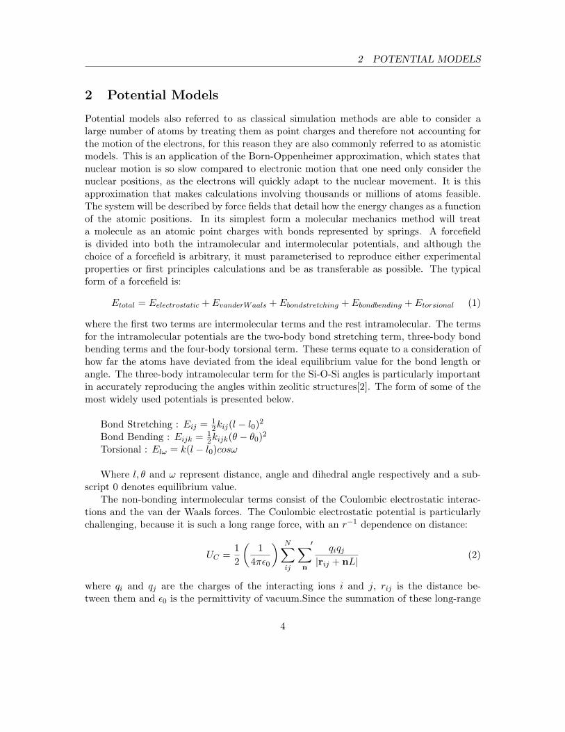
An additional level of sophistication may be added by employing the Dick and Over-hauser shell model to reproduce the polarisability of the oxygen ion within zeolites. Inthis model the the nucleus and the electron cloud are approximated as core and shell pointcharges connected by a harmonic spring [3]. This model improves the accuracy of the cal-culation, however as it splits each oxygen point charge in two it increases the complexityof the calculation and thus the time needed to complete it.

Figure 1: The shell model

5

3 AB INITIO METHODS

3 Ab Initio Methods

Ab Initio is a Latin term meaning from the beginning. A calculation is said to be ”ab initio”(or ”from first principles”) if it relies on basic and established laws of nature withoutadditional assumptions or special models, this sets these methods apart from so calledempirical methods which rely on experimentally determined parameters to calculate theproperties of the system being studied.

For example, an ab initio calculation of the properties of liquid water might start withthe properties of the constituent hydrogen and oxygen atoms and the laws of electrody-namics. From these basics, the properties of isolated individual water molecules would bederived, followed by computations of the interactions of larger and larger groups of watermolecules, until the bulk properties of water had been determined. Whereas a ”classicalmechanics” or empirical calculation would treat the water a series of point charges con-nected and interacting through a series of potentials which have been parameterized to fitto experimental data.

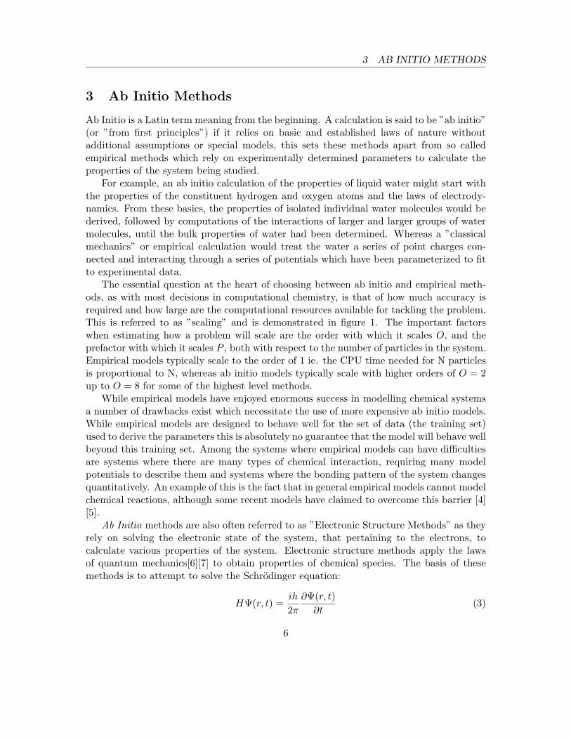
The essential question at the heart of choosing between ab initio and empirical meth-ods, as with most decisions in computational chemistry, is that of how much accuracy isrequired and how large are the computational resources available for tackling the problem.This is referred to as ”scaling” and is demonstrated in figure 1. The important factorswhen estimating how a problem will scale are the order with which it scales O, and theprefactor with which it scales P , both with respect to the number of particles in the system.Empirical models typically scale to the order of 1 ie. the CPU time needed for N particlesis proportional to N, whereas ab initio models typically scale with higher orders of O = 2up to O = 8 for some of the highest level methods.

While empirical models have enjoyed enormous success in modelling chemical systemsa number of drawbacks exist which necessitate the use of more expensive ab initio models.While empirical models are designed to behave well for the set of data (the training set)used to derive the parameters this is absolutely no guarantee that the model will behave wellbeyond this training set. Among the systems where empirical models can have difficultiesare systems where there are many types of chemical interaction, requiring many modelpotentials to describe them and systems where the bonding pattern of the system changesquantitatively. An example of this is the fact that in general empirical models cannot modelchemical reactions, although some recent models have claimed to overcome this barrier [4][5].

Ab Initio methods are also often referred to as ”Electronic Structure Methods” as theyrely on solving the electronic state of the system, that pertaining to the electrons, tocalculate various properties of the system. Electronic structure methods apply the lawsof quantum mechanics[6][7] to obtain properties of chemical species. The basis of thesemethods is to attempt to solve the Schrodinger equation:

HΨ(r, t) =ih

2π∂Ψ(r, t)∂t

(3)

6

3 AB INITIO METHODS

Figure 2: CPU time versus number of particles for a series of orders O and prefactors P ;Time = PNO.

where H is the Hamiltonian operator of the system, which is represented by the wavefunction Ψ, and which has a probability distribution |Ψ2|, this is the probability that thesystem will be in a given state. If we consider that the systems potential energy, V , is timeindependent, we obtain the time-independent Schrodinger equation:

HΨ = EΨ (4)

in which the energy E is the eigenvalue of the Hamiltonian operator. To aid calculationthese eigenvalues, the systems Hamiltonian can be split up into different contributions, theHamiltonian for this equation is:

H = T e(r) + Tn(R) + V n−e + V e(r) + V n(R) (5)

where the superscripts n and e refer to the nucleus and electrons respectively, V is potentialenergy, T is kinetic energy and R and r refer to nuclear and electron position respectively.A number of approximations are necessary if we are to solve the Schrodinger equation.The first important approximation which is made is the Born-Oppenheimer (BO) approx-imation. The BO approximation is that given that electrons are much lighter than thenucleus and therefore move much more rapidly the motions of the nucleus and electronscan be decoupled, the electrons are assumed to be always equilibrated and thus forces onthe nuclei arise only as a result of atomic positions. Thus the electronic structure part of

7

3.1 Hartree-Fock 3 AB INITIO METHODS

the problem is reduced to that of solving the time-independent Schrodinger equation, withthe electrons assumed to be in the ground state. This removes the second term from theabove equation, yielding the electronic Hamiltonian, He.

The next approximation necessary relates to the wave function and is called the ”LinearCombination of Atomic Orbitals” (LCAO) approximation. Essentially we assume that thetotal wave function Ψ, can be represented by a summation of smaller functions called basisfunctions φ :

Ψ =∑i

ciφi (6)

where φi are the atomic orbitals and ci is a factor weighting their overall contribution to themolecular orbital (MO), Ψ. The choice of the set of basis functions, called the basis set, tobe used in a calculation is of crucial importance in electronic structure calculations. Thisrelates to both the form of the basis functions and also to the number of functions to beused. The minimum amount of basis functions to be used is that which can accommodateall the electrons of the system, however for more accurate and sophisticated calculationsbasis functions representing unoccupied orbitals must be employed, once again which basisset to use boils down to a question of accuracy versus computational resources available.

We can now consider two of the major electronic structure methods , Hartree-Fock andDensity Functional Theory.

3.1 Hartree-Fock

Since we do not know the exact ground state solution, to solve the Schrodinger equationwe have to obtain the set of constants ci, using the variational principle, which statesthat the calculated energy will always be higher than exact solution. Hartree-Fock usesthe variational principle to obtain the constants, ci which allows us to solve the Roothanmatrix equation,

FC = SCε (7)

det|F − εaS| = 0 (8)

where F is the Fock matrix, C is the matrix of constants ci, S is the matrix of theoverlap orbitals and εa is the matrix of the energy levels of the system. The Hartree-Fockmethod utilizes a Self-Consistent Field (SCF) procedure to solve the variational principleequations. In an SCF the first calculation involves an educated guess for the values ofci, this is then used for a calculation of the Fock matrix, the resulting Fock matrix isthen used to generate a new better set of coefficients, this is repeated until the differencebetween the new and the old fock matrices is below a certian threshold value, called theconvergence criterion. This procedure is represented schematically in figure 3. The choiceof convergence value is another important consideration when setting up a calculation.

8

3.2 Post Hartree-Fock Methods 3 AB INITIO METHODS

Figure 3: A Schematic Representation of The Hartree-Fock SCF Procedure.

3.2 Post Hartree-Fock Methods

The Hartree-Fock method suffers from the fact that it approximates the many electronproblem as a one electron problem and implies that each electron sees the other electronsas a mean-field. Many attempts have been made to include electron correlation effects inelectronic structure calculations.

The configuration Interaction (CI) method takes into account mixing of possible elec-tronic states of the molecule in the form,

Ψ = b0Ψ0 +∑s

bsΨs (9)

where b0Ψ0 is the Hartree-Fock expression and the second term on the RHS takes intoaccount substitutions of virtual or excited states for occupied orbitals.

Another approach is the Møller-Plesset theory (MP)[8]. MP uses a perturbation onHartree-Fock theory, to remove the error that was introduced in Hartree-Fock theory whenthe two electron integrals were replaced by a one electron potential. The two electronintegrals are restored. Perturbation theory makes use of expanding the equation in a Taylorseries with respect to the Lagrange multiplier λ. The new Hamiltonian is

H = H0 + λV (10)

where H0 is the Hartree-Fock Hamiltonian. Expanding up to the first order gives theHartree-Fock solution. Including second order corrections leads to MP2. MP3 and MP4

9

3.3 Density Functional Theory (DFT) 3 AB INITIO METHODS

are also commonly used methods. The MP series does not often converge, because in goingfrom MP2 to MP3 and on to MP4, one does not necessarily get better approximations tothe ground state wave function. This is because perturbation theory is not variational,and thus a calculated energy is not necessarily an upper bound to the true ground stateenergy.

Post Hartree Fock methods, however, are often simply not practical for calculations.For a system of N atoms MP2 and MP4 scale as N5 and N7 respectively while CI methodsCISD and CISD(T) scale as N6 and N8 respectively. Compared to N4 scaling for Hartree-Fock calculations [9].

3.3 Density Functional Theory (DFT)

The central focus of DFT is the electron density,ρ and not the wave function as in Hartree-Fock methods. It is called a functional theory as the energy is a function of the density,E[ρ], which in turn is a function of the position, ρ(r). A functional is a function of afunction. The attraction of DFT is that it provides better results than Hartree-Fock, inmany cases comparable with the MP methods, whilst scaling as N4.

The basis for DFT is the Reductio ad absurdum1 by Hohenberg and Kohn[10] that theground state electronic energy is completely defined by the electron density, ρ, this proofis provided in an appendix. The foundation for the use of DFT methods in chemistry isthe introduction of orbitals as suggested by Kohn and Sham (KS)[11]. Within these DFTformalisms the energy is split up as follows:

EDFT [ρ] = Ts[ρ] + Ene[ρ] + J [ρ] + Exc[ρ] (11)

with Ts[ρ] the electron kinetic energy, Ene[ρ] the potential nuclear-electron interaction en-ergy, and J [ρ] the potential electron-electron interaction energy, the final term Exc[ρ] is theexchange-correlation energy which is calculated with an exchange-correlation functional.The choice of this last functional is where different DFT methods diverge and is crucial tothe success of the method.

In the simplest cases the functional is the Local Density Approximation, this approx-imation however tends to break down if the electron density is not close to homogenous.The next level of approximation is the Generalized Gradient Approximation (GGA) whichincludes the first derivative (the gradient) of electron density when calculating Exc[ρ].Commonly known GGA methods include PBE[12] and B88[13]. After GGAs are the meta-GGAs which include second derivatives of electron density in calculations. Finally thereare also what are known as hybrid functionals, which include a certain percentage of theexact exchange from Hartree-Fock theory. The most widely used, and very successful, hy-brid functional, is B3LYP[14, 15]. The major criticism of hybrid DFT methods is that the

1Reductio ad absurdum: the premise that something impossible is actually true, and then proving it isludicrous.

10

3.3 Density Functional Theory (DFT) 3 AB INITIO METHODS

percentage of HF exchange used is defined by a parameter obtained by fitting to experi-mental data, so for example B3LYP which was parameterized based on heats of formationworks well for energies but not necessarily well for other properties such as nuclear shieldingconstants.

All DFT functionals have problems reproducing physical and intermolecular interac-tions, like the van der Waals force. The reason for this misbehaviour is the incorrectasymptotical behaviour of the DFT interaction energy between multiple closed shell sys-tems. DFT is a local or short-range potential, whereas intermolecular interactions arelong-range. Corrections have been proposed to enhance the ability of DFT to model dis-persion forces such as the DFT:MP2 hybrid approach[16]. Improvements for modellingdispersion have also been proposed by the group of Lundqvist and Langreth [17], thesecorrections are based on a double local density approximation. Yet another method forimproved modeling of dispersion is the use of a damped dispersion function[18],

Etot = EDFT + EDisp (12)

with EDisp given by a dispersion function which is dampened to remove unrealistic behaviorat small distances.

11

4 CHALLENGES IN MOLECULAR MODELING

4 Challenges In Molecular Modeling

The methods described thus far have been hugely successful when calculating the propertiesof systems in the gas phase at zero kelvin, however this clearly represents only a very smallsubspace of the chemical reactions and systems of interest practically. In order to be ableto model ”real-life” systems a number of ingenious methods have been developed, only asmall fraction of which will be considered here. The two major challenges with which weshall deal here are those of molecules in solution and the search for the absolute minimumenergy of chemical systems.

4.1 Molecules In Solution

When representing solvation two approaches are available, one is to model the solventimplicitly, ie to include the solvents effects directly when solving the Schrodinger equationof the system. The second is to include the solvent explicitly, ie. to include actual moleculesof solvent surrounding the system of interest, of these two methods the second provides aphysically more realistic scenario, however it introduces extra particles into the system, andgiven scaling constraints can quickly become infeasible as the number of solvent moleculesrises. It is also possible to consider a hybrid of the two methods in which the molecule issurrounded by one layer of solvents which in turn includes an implicit model.

4.1.1 Implicit Solvation

The origins of an implicit model for solvation effects can be traced back to Born (1920) andOnsanger (1936). Born[19] derived the free energy of solvation for placing a charge withina spherical cavity in a solvent, Onsanger [20] extended this to a dipole within a sphericalcavity. The Born model calculates solvation energy as the work done in moving a pointcharge from vacuum to a spherical cavity within a continuum. It is an extremely simplemodel however can be effective in the case of the solution of ions.

The Onsanger model is appropriate for many more species, in this model the solutedipole in side a cavity is considered. The dipole of the solvent induces a dipole in thesurrounding continuum, which results in an electric field inside the cavity, this is called areaction field. The reaction field then interacts with the solute dipole providing additionalstabilization for the whole system. The reaction field model can be incorporated intoquantum mechanical calculations where it is commonly known as the ”Self ConsistentReaction Field” (SCRF) model. The SCRF model has been refined by Menucci and co-workers [21, 22] to use a cavity of the shape of the molecule which is built from a series ofspheres centred on each atom, the solute charge is then represented as a series of chargepoints spread out on the resulting cavity surface.

SCRF models have been applied successfully to investigate the effects of solvation inmany chemical systems and for various properties, however there are certain cases for whichthe continuum representation of the solvent is not sufficient, for example if hydrophobic

12

4.1 Molecules In Solution 4 CHALLENGES IN MOLECULAR MODELING

effects are present the continuum model will not represent them, another example is wherespecific solvent-solute interactions are important such as hydrogen bonding in water. Insuch cases it may be necessary to use explicit methods.

4.1.2 Explicit Solvation and Perdioc Boundary Conditions (PBCs)

If one is to model solvation explicitly by including ”real” solvent molecules then an ob-vious question arises, how many explicit solvent molecules are necessary for a realisticrepresentation, as the solvent molecules are obviously themselves ”solvated” by other sol-vent molecules and these effects may be of importance. In some respect by including onlya finite number of solvent molecules one is in effect only modeling a bubble of moleculeswithin a vacuum. An elegant and relativly simple solution to this problem is to use PeriodicBoundary Conditions (PBCs). This allows a relatively small number of particles to behaveas if they are part of a bulk system. The molecules are placed inside a cubic box of givendimensions, this box is then surrounded by identical boxes and so on, a 2D representationof this system is given in figure 4. The coordinates of the particles in an image box cansimply be calculated by adding or subtracting an integer to the coordinates of the originalbox, should a particle leave the box it will be replaced by its image entering from the otherside, thus the contents of the box remain constant. As represented by the dashed lines in

Figure 4: A representation of a 2D system surrounded by periodic images.

figure 4 the particles in the original box now interact with particles all around them, allof this is achieved with relatively little computational cost, an certainly not of the order ofjust adding the extra molecules.

13

4.2 Energy Minimization 4 CHALLENGES IN MOLECULAR MODELING

It should be noted that the use of PBCs is not restricted to liquid phases, indeed thetechnique was developed in the solid state modeling community and is particularly usefulwhen modeling crystal structures as a periodic repetition of a basic unit cell, see sections4.3 and 5.

4.2 Energy Minimization

The energy minimization problem is this: given a system with energy E which dependson independent variables x1, x2, . . . , xi, find the values of xi for which E is a minimum.At a minimum point the first derivatives with respect to xi of E are zero and the secondderivatives are positive:

∂E

∂xi= 0;

∂2E

∂x2i

> 0 (13)

For standard analytical functions these values may be found by calculus methods, howevergiven that the energy in chemical systems is dependent on the cartesian coordinates of theatoms involved the energy functions of interest are much more complex and must be foundby numerical methods. Numerical methods in principle involve varying the coordinatesuntil these conditions are met. This still seems like a simple enough proposition, howeverthere exists another, more challenging problem, as represented in figure 5, it is this, ina potential energy landscape there generally exists more than one point where the criteriafor a minimum are met. In this case we have both local and global minima, the globalminimum being the minimum of the minima. The question now is how can we be surethat the minimum which we have found is a global minimum. The answer in short is wecan’t, not without exploring the full energy landscape. However if we can be sure that wehave sampled enough of the potential energy landscape then we can be confident in ourglobal minimum. So now we must sample the energy landscape to a suitable extent, thisis not a trivial problem given the expense incurred in electronic structure calculations. Inmany cases it is more practical to sample the energy landscape using cheaper molecularmechanics methods followed by an electronic structure refinement of the lowest energyconfigurations from these calculations. However as computer resources improve and moresophisticated and cost effective electronic structure methods are developed the goal of fullenergy landscape exploration by Ab Initio methods is becoming more feesible. As moleculardynamics have been dealt with else where we will not look at them here but rather exploreyet another restricting factor in energy landscape sampling.

This sampling problem is confounded by the energy barriers which exist in the energylandscape, it is entirely possible that during the course of a dynamics simulation a systemmay become stuck in an energy well which is not the global minimum, but which has anenergy barrier too high to allow escape. There are many methods to overcome this issuein the next section we will look at one of the more recent and promising approaches.

14

4.2 Energy Minimization 4 CHALLENGES IN MOLECULAR MODELING

Figure 5: A 2D schematic representation of the global versus local minimum problem.

4.2.1 Molecular Dynamics (MD)

The energy minimisation technique does not take into account the kinetic energy of thespecies. It gives good results for the system with a temperature of zero Kelvin, eventhough the zero point energy is neglected. However, this approach does not include theinfluence of the temperature, therefore the system does not evolve in time and is likely tostay in the local minimum of energy. In the molecular dynamics method, the species havekinetic energies and therefore can mimic the situation of a real experiment in a better way.The system is not trapped in the local minimum but can evolve to reach a more stableconfiguration.

An MD simulation is performed in repetitive steps. However, firstly the starting config-uration of the system needs to be set up. The positions of ions are initially obtained froma simple minimisation and velocities are given randomly with a distribution producing therequired simulation temperature.

The next step is to calculate the force applied to each of the particles. It is obtainedfrom the interaction energy U(ri), provided by the potential model:

Fi = −∇U(ri) (14)

Having the forces, the new particle positions and velocities are obtained from the Newton’sequations of motion:

ai(t) =Fi(t)mi

(15)

15

4.2 Energy Minimization 4 CHALLENGES IN MOLECULAR MODELING

The numerical solution of these equations leads to the scheme:

vi(t+ δt) = vi(t) + ai(t)δt (16)

ri(t+ δt) = ri(t) + vi(t)δt (17)

where ai, vi and ri are acceleration, velocity and position of ion i, respectively, and δt isthe time step. The value of the time step δt determines the accuracy of the result, whenit tends to zero the approximated solution tends to exact value. However, if the time stepis too small the CPU time of the calculation is too long. In practice, the δt value is acompromise between accuracy and speed of the simulation. The size of δt is limited bythe frequencies of the molecular vibrations occurring in a modelled system – the time stepmust be less then reciprocal of the highest frequency. Every step, after the new positionsand velocities are obtained, the properties of the system are calculated. In the first severaltens of time steps, the equilibration period is performed. This is necessary because theinitial positions and velocities are usually far from the equilibrium ones and, therefore, inthis period the velocities are scaled to obtain the required temperature.

4.2.2 Monte Carlo

Monte Carlo (MC) methods unlike MD are not a deterministic technique, instead makinguse of random numbers to perform random moves and orientation changes to generatesuccessive configurations. The particular advantage of MC methods is that completelyunrelated configurations are generated, so it is potentially possible for the entire region ofphase space to be sampled. By comparison MD methods may only sample a very smallportion of the phase space close to the starting configuration unless the simulation is runfor a long time or special techniques are used to overcome barriers. The simplest formof a MC simulation accepts any new configuration with a lower energy than the previousconfiguration, however this is an inefficient way to sample the system, since high and lowenergy states are generated with equal probability. Therefore sophisticated MC methods,such as the Metropolis algorithm, make use of importance sampling to ensure that themajority of the time is spent sampling the low energy configurations that are of mostinterest. In order to do this the configurations are weighted by the Boltzmann factor,β =exp(−∆v/kbT ), which ensures higher energy configurations have a lower probability ofbeing sampled. The Metropolis algorithm will ensure that each step only depends on theconfiguration of the previous step and not on any earlier configurations, hence generatingwhat is known as a Markov chain of states. Figure 6 is a schematic which demonstratesthe Metropolis Method. When a trial move is made through the calculation of a randomtranslation in each of the x, y and z coordinates, the energy is calculated and hence thechange in energy, ∆v = En − Em, from the previous configuration. If ∆v is negative thenthe move is automatically accepted as it is downhill. If ∆v is positive then the Boltzmannfactor, β, is compared to a random number between 0 and 1. If the Boltzmann factor

16

4.2 Energy Minimization 4 CHALLENGES IN MOLECULAR MODELING

is greater than the random number then the move is accepted, otherwise it is rejected.This process is then iterated. The greater the temperature (i.e. the greater the thermalenergy) of the system, the more likely it is that an uphill move will be accepted, since theBoltzmann factor is larger.

Figure 6: Schematic demonstrating how a Metropolis algorithm performs a MC simulation.

4.2.3 Metadynamics[1]

Traditional Molecular Dynamics and Monte Carlo methods have had a great impact inmany fields, however due to computational costs there exist many systems for which”straight-forward” dynamics simply cannot explore the full landscape, consider the land-scape presented in figure 5. If the system were to become trapped in the local minimumwell, and did not have sufficient energy to overcome the barrier to get out the resultantsimulation would sample only a small subspace of the system configurations and wouldmiss the global minimum. In a traditional dynamics the configuration would propagateaccording to an equation something like:

σt+1i = σti + δσ

φ

|φ|(18)

in which σti represents the configuration at time t, and the second term on the right handsize is related to calculating the force on the system. If this force becomes too great asthe system attempts to leave the energy well it will simply slide back down the side ofthe well and not sample the space beyond this. The idea behind metadynamics is to buildinto this force a history dependent term, a kind of memory in order to avoid resamplingconfigurational spaces. this is achieved by placing small gaussian functions at points whichhave already been visited, this is illustrated in figure 4.2.3 (a). The result is that asthe calculation continues the wells become filled with these gaussian functions and the

17

4.3 Modeling Surfaces 4 CHALLENGES IN MOLECULAR MODELING

energy land scape flattens out, 4.2.3 (b). The metadynamics procedure at the same timeas allowing escape from local minima also provides for a backwards analysis to reveal theoriginal energy surface, thus no information is lost and sampling power is greatly increased.

Figure 7: (a) on the left the energy profile being filled with small gaussian (red), (b) theenergy profile becoming increasingly flattened as the simulation proceeds (thin lines).

4.3 Modeling Surfaces

A key part of understanding zeolite crystal growth is to look at what is happening at thesurfaces. To model the processes occurring at surfaces we first need to have a reasonablemodel of the process. Since we are considering a crystalline (i.e. periodic) solid we willautomatically require the use PBCs. There are 2 key ways we can model a surface:

1) Periodic (3D): Use PBCs in all three dimensions. It will consist of a slab (continu-ous in, say, the x and y directions) with a vacuum or some other medium between the topand bottom surface in the z direction. The size of the medium gap between the top andthe bottom of the slab must be sufficiently large that the two surfaces are not chemicallyaware of each others presence.

2) Aperiodic (2D): Use PBCs only in the plane of the crystal (eg. x and y plane).In both cases you need to ensure that your slab is the correct size. For example, imagine

modelling a molecule approaching a zeolite surface, and you are using a 3D periodic cell torepresent this surface. If the crystal slab is too thin, then the molecule will not only interactwith the top surface, but also with the bottom surface. However we do not want to makeany slab excessively thick as this will increase the computational expense of modelling thesystem.

When we create a surface we will be starting from a model of the materials bulk unit cell,most often the coordinates used are those characterised by an experimental technique, eg.XRD. For zeolites we rarely have as much information on the exact nature of its surfaces,

18

4.3 Modeling Surfaces 4 CHALLENGES IN MOLECULAR MODELING

Figure 8: A representation of the two methods for surface representation; a) 3D periodic;b) 2D periodic.

although any information from HRTEM or other surface characterisation techniques isinvaluable. Starting from the bulk unit cell we consider all the possible surface terminationsfor a particular plane. The most stable surface termination is particularly interesting sincewe can expect this to be the longest lived termination, hence its growth will determinethe RDS of that surfaces growth and it is what we expect to be observed experimentally.Obviously, depending on what we are trying to model, it is often necessary to look at otherviable surfaces as well. As a simple rule the most stable surface should be the surface thatrequires the least chemical bonds to be broken when it is cleaved from the bulk cell (as themore dangling bonds a surface has the less stable it would be). Another more subtle pointis that a surface should be chosen so as to minimise/remove any dipole running across it(a dipole that does not exist in the true crystal, but is created merely by the making ofthe surface model).

19

5 CASE STUDY: ZEBEDDE

5 Case Study: ZEBEDDE

The computer program ZEBEDDE (Zeolites By Evolutionary De Novo Design) was de-veloped by Lewis and Willock in 1996 with the aim of predicting templates for a givenzeolitic structure[1,2,3]. The principle being that the better the fit of a molecule withinthe framework the better that molecule will actually template to a particular structure.The program was designed to build a template from scratch (de novo); the procedure usedis summarised as follows; the program places a small fragment (seed) within the void ofa zeolite (termed the host) and then carries out a series of actions upon this guest. Theseactions are:

[1] BUILD add on a new fragment (from a library of possible fragments).

[2] ROTATE rotate the last bond added.

[3] SHAKE move the guest a random distance (between set limits) in a random direc-tion.

[4] ROCK rotate the guest a random amount.

[5] RING FORMATION take two end atoms and join them to form a ring.

[6] MINIMISE GAS PHASE Perform an energy minimisation (as if the zeolite host wasnot visible to the guest molecule).

[7] MINIMISE IN HOST Perform an energy minimisation (with the zeolite host visibleto the guest molecule).

[8] TWIST this is a recent addition to ZEBEDDE that rotates a randomly selectedbond.

When an action is carried out it can be testing to find out whether it is an improvementby comparing the current and previous energy, to see whether the action has resulted ina reduction in energy (i.e. it is an energy minimisation tool, see Section 4.2 ). Morerecently a Monte Carlo function was added into ZEBEDDE. This can be chosen instead ofthe energy minimisation so that the simulation can overcome energetic barriers (considerFigure 5 ).

ZEBEDDE is an atomistic technique (see Section 2 ), this is necessary because itneeds to carry out typically 1000+ actions and often each simulation would need to berepeated many times to ensure you had sampled all possible answers. It would be too timeconsuming using electronic structure methods and this level of accuracy is not deemednecessary for the task of testing the fit. ZEBEDDE requires PBC (Section 4.1.2 ) to

20

6 CASE STUDY: KINETIC MONTE-CARLO METHOD

be able to model the zeolite (since it is a periodic solid). To calculate the electrostatic(Coulombic) interactions it makes use of the Ewald summation method (Section 9 ),necessary due to the PBCs.

There are many of simulation parameters that can be used to affect how the simulationruns, for example: the fragments available for addition, the bias towards the addition atcertain sites (ie. to influence the amount of branched vs linear molecules that would begrown), the minimisation tool used (for Actions 6 7), the bias towards certain actions overothers, how often an action is accepted without testing etc etc.

ZEBEDDE is not limited to being used for the growth of templates. It may also justbe used to take a given template and then carry out actions (only 3,4,6,7,8) so as to findthe most energetically favourable position for the template within a particular void or on asurface (using a 3D periodic cell, see Section 4.3). Similarly ZEBEDDE does not have tobe carried out on a zeolite and template, it can be used for any guest molecule within/ona host.

6 Case Study: Kinetic Monte-Carlo Method

6.1 The Model

The kinetic monte-carlo method randomly chooses a particular growth site based on certainprobabilities, and the number of that particular site which are available, and adds a growthunit to this site. Using these probabilities the program can then be applied to calculatethe rates, activation energies and Free energies of crystal growth. As we have substantialinformation realting to Zeolite A we have chosen this as our prototype model.

Thus far one type of growth unit has been implemented in the program in order tomodel the following:

• Zeolite A crystal growth program in 3D.

• Zeolite A crystal growth and dissolution program in 3D

• Zeolite A crystal growth and dissolution program on (100) face in 2D (monolayerspreading growth)

• Zeolite A crystal growth and dissolution program on (110) face in 2D (monolayerspreading growth)

The growth unit is modeled as 1.2nm cubes, which corresponds to the experimentallydetermined terrace height in zeolite A, comprising a sodalite cage and double four ring(D4R).

The simulation performs one growth unit addition or dissolution per iteration, and thenupdates the site type of the 24 nearest neighbors of the site which has been affected. The

21

6.2 Development 6 CASE STUDY: KINETIC MONTE-CARLO METHOD

Figure 9: (a)Each cube shows a growth unit. Growth/dissolution site (pink) is surroundedby 6 nearest neighbours (green) and 18 second nearest neighbours (purple). (b) The Kosselmodel.

nearest neighbor sites are categorized as having either first or second sphere coordinationto the affected site see Figure 9 (a) The chosen growth/dissolution site has six nearestneighbours, which have 5 categories corresponding to the Kossel model (Fig ??) . Inorder to generate bevelled edges (ie, 110 faces) and/or corners (ie, 111 faces) of a cube, thesecond nearest neighbours are also considered. This results in 223 possible ”site types” orcategories, however for simplicity we consider only the six key site types.

6.2 Development

The challenge for the program is to control both morphology and topology using a cer-tain set of probabilities. In 3D, although crystal morphology could be controlled,topologyneeded a certain shape to be more realistic.

6.2.1 Zeolite A crystal growth and dissolution program in 3D

The problem was it was hard to treat 192 site types (excluding bulk) to control the morphol-ogy and topology at the same time. Also, the small limited computer memory environmentcaused a further difficulty to compare simulation images with real crystal images. Hence,2D simulation program on (100) face was created to cope with above problems.

6.2.2 Zeolite A crystal growth and dissolution program on (100) face in 2D

The simulation was focused on mono-layer surface spreading (ie, the top of the surfaceterrace is supposed to be simulated). NB: multi-layer shows 3D because the second nearestneighbours are considered. As a result, we could say the curved corners were generatedunder the dissolution; however, to decide the certain probability set, we need more data

22

6.2 Development 6 CASE STUDY: KINETIC MONTE-CARLO METHOD

(eg, more real images and their size of radius at the corner (Fig,3), and also the ratiobetween growth rate and dissolution rate).

6.2.3 Zeolite A crystal growth and dissolution program on (110) face in 2D

Zeolite A crystal growth and dissolution program on (110) face in 2D As we have observedthe (110) faces by means of AFM and SEM, the 2D simulation program for (110) face wasalso created to decide the (110) surface topology by a certain probability set.

Probability sets generated by the 2D programs will be applied for probability sets onthe 3D program, considering the ratio of site types to make the crystal morphology as wellas surface topology.

23

7 APPENDIX A: PROOF OF THE HOHENBERG-KOHN THEOREM

7 Appendix A: Proof of the Hohenberg-Kohn Theorem

The Hohenberg-Kohn theorem demonstrates that there is a functional relationship betweenthe electron density, ρ, and all observable properties of the interacting system of particles,meaning that all properties of the system may be determined if the electron density isknown. We start by assuming that there exist two different potemtials v and v′ which yieldthe same electron density ρ, these two external potentails generate different operators Vand V ′ which in turn yield two different Hamiltonians H and H ′. These systems also willhave different wave functions Φ and Φ′ with energies E and E′ the energies are given by :

E = 〈Φ|H|Φ〉 (19)E′ = 〈Φ′|H ′|Φ′〉

Now by applying the variational principle we can say that the exact Hamiltonian for asystem always yields lower energy than an approximate one thus:

E′ = 〈Φ|H|Φ〉 < 〈Φ|H ′|Φ〉 (20)E = 〈Φ′|H ′|Φ′〉 < 〈Φ′|H|Φ′〉

We can also say that

〈Φ|H ′|Φ〉 = 〈Φ|H + V ′ − V |Φ〉 (21)〈Φ′|H|Φ′〉 = 〈Φ′|H ′ + V ′ − V |Φ′〉

assuming that〈Φ′|ρ|Φ′〉 = ρ(r) = 〈Φ′|ρ′|Φ′〉 (22)

which is our original assumption, we obtain that

E′ < 〈Φ|H|Φ〉+∫dr[v′(r)− v(r)]ρ(r) = E +

∫dr[v′(r)− v(r)]ρ(r) (23)

E < 〈Φ′|H ′|Φ′〉+∫dr[v(r)− v′(r)]ρ(r) = E′ +

∫dr[v(r)− v′(r)]ρ(r)

Adding these two inequalities yields:

E′ + E < E + E′ (24)

This result is inconsistent and thus proves that the original assumption is false.

24

8 APPENDIX B: BASIS SETS

8 Appendix B: Basis Sets

It would be negligent when introducing Ab Initio methods to overlook an explanation ofbasis sets, which after the choice of method are the most important factor in setting up acalculation, and a continual source of controversy and debate.

As stated earlier basis sets are sets of basis functions which are combined to give awave function. There exist two major types of basis sets, plane wave basis sets and atomcentred basis sets. We will concentrate primarily on the latter as they are more commonlyused in liquid and gas phase calculations. Atom centred basis sets are comprised of atomicfunctions representing the electron population at a given distance from the nucleus andcan be thought of as being atomic orbitals. There are a number of different types of atomcentred basis functions available. One obvious choice are Slater type orbitals (STOs) whichare of the form:

R(r) = Nrn−1e−ζr (25)

where n is the principal quantum number, N is a normalization constant, r is the distancefrom the nucleus and ζ is a constant related to the atomic charge of the nucleus. Un-fortunately STOs are often impractical for quantum chemical calculations as some of theintegrals are difficult or even impossible.

By far the most popular type of basis sets used in quantum chemistry are those basedon Gaussian functions, Gaussian type orbitals (GTOs), these have the form:

R(r) = xaybzce−αr2

(26)

α determines the spread of the function, r is the distance from the nucleus, x, y, z arecartesian variables and a, b, c determine the order of the function. If a+ b+ c = 0 then thefunction is zeroth order, and one such function exists, if a+ b+ c = 1 the function is firstorder and three such functions exist, zeroth order functions are equivalent to s orbitals,first order functions to px, py and pz orbitals and so on up the orders.

A minimal basis as stated earlier is that which contains just enough functions to ac-commodate all of the electrons present., however as stated earlier in practice minimal basissets are often not good enough for the task at hand. The basis set can be expanded in anumber of ways. One way is to split each of the functions in the basis set, if the functionsare split once this is known as a double zeta basis set, basis sets up to quadruple zeta arecommonly used. An alternative approach which is highly popular is to split only the basissets used for valance electrons, the rational being that the chemical properties of interestare effected by the valance rather than the core electrons, this approach is known as thesplit valance approach and is so popular that it has its own notation, exemplified by thelabel 3-21G, this means that core electrons are teated with 3 functions, whilst valanceelectrons are treated with functions split into two contracted Gaussians and one diffuseGaussian. Popular examples of this type of basis set are 3-21G, 4-31G and 6-31G.

Simply increasing the number of basis functions may not necessarily improve the model,and there are other issues which must be considered when issues such as orbital mixing

25

9 APPENDIX C: EWALD SUMMATION

are involved, for example in an isolated hydrogen atom the electron cloud is spherical,however as the atom approaches another hydrogen atom this becomes distorted and thecloud takes on some p orbital character or is said to be sp hybridized. in order to account forthis we introduce what are called polarization functions. Polarization functions have higherangular quantum numbers, thus the polarization function for a hydrogen atom correspondsto a p orbital function, and to a d orbital function for first and second row atoms. Theuse of polarization functions is denoted by an asterix. Hence the 6-31G basis with addedpolarization is the 6-31G* basis set.

A final complication which we will consider is that of species with lone pairs of electrons.These lone pairs reside far away from the nucleus and are poorly represented by Gaussianfunctions, as they decay quickly when moving away from the nucleus. The solution to thisis to add highly diffuse functions. These are denoted by a +, so the 6-31G* basis set withadded diffuse functions for heavy atoms is denoted 6-31+G*.

When modeling periodic systems basis sets of the lane wave form are usually chosen,the general form of such basis sets is:

ψ(r) =∑G

aGexp(i(k +G)r) (27)

In this case the basis function is continuous and not centred on the atom as with gaussiantype basis sets.

There exist many other types of basis sets and methods for improving them, howeverfor the purposes of this introductory document it is considered sufficient to discuss onlythe most commonly encountered basis sets.

9 Appendix C: Ewald Summation

The sum in equation 2 converges slowly because the electrostatic potential, due to pointcharges, decays as 1/r. The way to overcome that was presented by Ewald [?]. In thismethod the density of point charges, represented by a sum of δ functions, is modified byan additional sum of diffuse charge distributions around each ion. The diffuse distributionis selected such that it is opposite in sign to the point charge and thus the total charge iscancelled out. As a result, the electrostatic potential due to a single ion is a fraction oforiginal potential that is not screened by diffuse charge. This remaining fraction rapidlyconverges to zero at long distances, which allows the use of a direct summation for thescreened charges. The screening charge distribution around ion i usually has the form of aGaussian

ρg(r) = −qi(απ

) 32 exp(−αr2) (28)

where r is position relative to the centre of the distribution and parameter α sets the widthof the distribution. The interaction energy due to the screened charge distribution can be

26

9 APPENDIX C: EWALD SUMMATION

calculated from following equation

U1 =12

(1

4πε0

) N∑ij

′∑n

qiqj|rij + nL|

erfc(√α|rij + nL|) (29)

where erfc is the complementary error function

erfc(x) = 1− 2√π

x∫0

exp(−t2)dt (30)

obtained by solving Poisson’s equation for Gaussian charge distribution. For large argu-ments this function tends to zero.

Figure 10: Scheme of the Ewald method; a) point charges; b) screened point charges; c)Gaussian charge distribution

The electrostatic potential due to screened charges does not describe the full interac-tion between point charges, therefore, a correction must be introduced. The method forcorrecting the interaction is shown in Figure 10. Point charges are surrounded by screen-ing charges and are then compensated by a charge distribution smoothly varying in space.As the compensating charge distribution is a periodic function it can be represented by a

27

9 APPENDIX C: EWALD SUMMATION

rapidly converging Fourier series. The density of the compensating charge is formulatedby a sum of Gaussians:

ρ1(r) =N∑j=1

′∑n

qj

(απ

) 32 exp

[−α|r− (rj + nL)|2

](31)

which in reciprocal space becomes:

ρ1(k) =1V

N∑j=1

qj exp(−ik · rj) exp(−k2

4α

)(32)

Applying Poisson’s equation yields the electrostatic potential:

Φ(k) =4πk2

1V

N∑j=1

qj exp(−ik · rj) exp(−k2

4α

)(33)

where k 6= 0. The reciprocal space contribution becomes:

Φ(r) =1V

∑k 6=0

N∑j=1

4πqjk2

exp[−ik · (r− rj)] exp(−k2

4α

)(34)

and the contribution to the interaction energy is equal to:

U2 =V

2

∑k 6=0

4πk2|ρ(k)|2 exp

(−k2

4α

)(35)

where ρ(k) is defined as:

ρ(k) =1V

N∑i=1

qi exp(−ik · ri) (36)

As equation 35 includes the interaction between the charge cloud around an ion and the ioncharge itself, another correction is introduced. The form of this self-interaction correctionis evolved to be

Us =(απ

) 12

N∑i=1

q2i (37)

and does not depend on ions positions.

Considering all contributions, the Coulomb interaction is given

UC = U1 + U2 − Us (38)

A detailed derivation of above equations can be found in Frenkel and Smit [23].

28

11 GLOSSARY OF PROGRAMS AND CODES

10 Glossary

De Novo DesignThe design of compounds by incremental construction of a model withina model of the crystal site.

Eigenvalue:A scalar value λ that permits nonzero solutions y in equations of the formLy = λy;where L is an operator and where y can represent a vector or a function that is subject

to certain boundary conditions (eg that y is zero at a certain point).Fock Matrix: Is defined by the Fock Operator, which is equivalent to a Hamiltonian

for a single electron in a poly-electron system.Hamiltonian: An operator representing the energy of the electrons and nuclei in a

molecule. The Hamiltonian operator acts on the wave function yielding the energy.Operator : a function, that operates on (or modifies) another function.Potential Energy Surface: A plot of the potential energy of a system in relation

to the parameters which define the potential energy. It can be visualized as a landscapein which the height changes with position, thus the energy would correspond tho heightand the variables would correspond to location on the north south east west grid. Forthis reason it is also commonly referred to as a potential energy landscape. In reality in achemical system the surface will be of more than three dimensions; given that each atomin the system has 3 degrees of freedom the surface will be in 3N dimensions, where N isthe number of atoms

Variational Principle: The expectation value of the Hamiltonian for a trial wave-function must be greater than or equal to the actual ground state energy. Or in otherwords:

Eground 6 〈φ|H|φ〉 (39)

By definition, the ground state has the lowest energy, and therefore any trial wavefunctionwill have an energy greater than or equal to the ground state energy.

Wave Function: A mathematical function for a state of a system, from a space thatconsists of the possible states of the system.

11 Glossary of Programs and Codes

Gaussian: A commercially available package for quantum and semi-empirical calcula-tions.

GAMESS: Essentially the same as Gaussian but open-source, so somewhat less pol-ished.

GULP: General Utility Lattice Program. Program to perform atomistic calculationsfor molecules and solids. It provides a variety of simulation approaches, mostly using

29

REFERENCES REFERENCES

analytical techniques, and can be applied to a variety of systems eg molecule, surface,periodic solid.

METADISE: Atomistic code for modeling surface structure and stability.SIESTA: Spanish Initiative for Electronic Simulations with Thousands of Atoms. Pro-

gram to perform electronic structure (Density Functional Theory) calculations and Molec-ular Dynamics simulations of molecules and solids.

Quickstep (cp2k): Open-source code using a mixture of gaussian and plane wavebasis sets for efficient molecular ab initio dynamics simulations of large systems.

ZEBEDDE: ZEolite By Evolutionary /De Novo/ DEsign. Program to design a tem-plate for a specific zeolite structure. In principle has wider use for locating/building any’guest’ within/on a ’host’.

References

[1] Laio, A. and Parrinello, M., Proceedings of the National Academy of Sciences, 2002,99(20), 12562–12566.

[2] Henson, N. J.; Cheetham, A. K. and Gale, J. D., Chemistry of Materials, 1994, 6(10),1647–1650.

[3] Dick, A. and Overhauser, B., Physical Reviews, 1958, 73, 90–103.

[4] Nielson, K.; vanDuin, A.; Oxgaard, J.; Deng, W.-Q. and Goddard, W., Journal ofPhysical Chemistry A, 2005, 109(3), 493–499.

[5] Cole, D. J.; Payne, M. C.; Csanyi, G.; Spearing, S. M. and Ciacchi, L. C., The Journalof Chemical Physics, 2007, 127(20), 204704.

[6] Szabo, A. and Ostlund, N., Modern Quantum Chemistry: Introduction to AdvancedElectronic Structure Theory 2nd ed., Dover Publications, 1996.

[7] Atkins, P. and Friedman, R., Molecular Quantum Mechanics 4th ed., Dover Publica-tions, 1996.

[8] Møller, C. and Plesset, M. S., Oct , (1934), 46(7), 618–622.

[9] Leach, A., Molecular Modelling Principles and Applications, 2nd Ed., Prentice Hall:Harlow, 2001.

[10] Hohenberg, P. and Kohn, W., Phys. Rev., 1964, 136.

[11] Kohn, W. and Sham, L., Phys. Rev., 1965, 140.

[12] Perdew, J.; Burke, K. and Ernzerhof, M., Phys. Rev. Lett., 1996, 77, 3865.

30

REFERENCES REFERENCES

[13] Becke, A., Phys. Rev. A, 1988, 98, 3098.

[14] Becke, A., J. Chem. Phys., 1995, 98, 5648.

[15] C. Lee, W. Yang, G. P., Phys. Rev. B, 1988, 37, 785.

[16] Tuma, C. and Sauer., J., Phys. Chem. Chem. Phys., 2006, 8, 3995.

[17] Hult, E.; Rydberg, H.; Lundqvist, B. I. and Langreth, D. C., Phys. Rev. B, 1999, 59,4708.

[18] Zimmerli, U.; Parrinello, M. and Koumoutsakos, P., The Journal of Chemical Physics,2004, 120, 2693.

[19] Born, M., Z. Physics, 1920, 1, 45.

[20] Onsanger, L., J. Am. Chem. Soc., 1936, 58, 1486.

[21] Miertu˘ s, S.; Scrocco, E. and Tomasi, J., Chem. Phys., 1981, 55, 117.

[22] Cances, E.; Mennucci, B. and Tomassi, J., J. Chem. Phys., 1997, 107, 3031.

[23] Frenkel, D. and Smit, B., Understanding Molecular Simulations, Academic Press, SanDiego, 1996.

31