An Introduction to Calculus: Limits, Derivatives, and ... · An Introduction to Calculus: Limits, Derivatives, and Integrals ... CHAPTER 10 An Introduction to Calculus: Limits, Derivatives,

791

An Introduction to Calculus: Limits, Derivatives, and Integrals

Windmills have long been used to pump water from wells,grind grain, and saw wood. They are more recently beingused to produce electricity. The propeller radius of thesewindmills range from one to one hundred meters, and thepower output ranges from a hundred watts to a thousandkilowatts. See page 800 in Section 10.1 for some more information and a question and answer about windmills.

10.1 Limits and Motion:The Tangent Problem

10.2 Limits and Motion: The Area Problem

10.3 More on Limits

10.4 NumericalDerivatives and Integrals

C H A P T E R 1 0

5144_Demana_Ch10pp791-838 1/13/06 3:18 PM Page 791

Chapter 10 OverviewBy the beginning of the 17th century, algebra and geometry had developed to the pointwhere physical behavior could be modeled both algebraically and graphically, eachtype of representation providing deeper insights into the other. New discoveries aboutthe solar system had opened up fascinating questions about gravity and its effects onplanetary motion, so that finding the mathematical key to studying motion became thescientific quest of the day. The analytic geometry of René Descartes (1596–1650) putthe final pieces into place, setting the stage for Isaac Newton (1642–1727) and GottfriedLeibniz (1646–1716) to stand “on the shoulders of giants” and see beyond the algebra-ic boundaries that had limited their predecessors. With geometry showing them the way,they created the new form of algebra that would come to be known as the calculus.

In this chapter we will look at the two central problems of motion much as Newton andLeibniz did, connecting them to geometric problems involving tangent lines and areas.We will see how the obvious geometric solutions to both problems led to algebraicdilemmas, and how the algebraic dilemmas led to the discovery of calculus. The lan-guage of limits, which we have used in this book to describe asymptotes, end behavior,and continuity, will serve us well as we make this transition.

792 CHAPTER 10 An Introduction to Calculus: Limits, Derivatives, and Integrals

10.1Limits and Motion: The Tangent Problem

Average Velocityis the change in position divided by the change in time, as in the

following familiar-looking example.

EXAMPLE 1 Computing Average VelocityAn automobile travels 120 miles in 2 hours and 30 minutes. What is its average veloc-

ity over the entire 2�12

� hour time interval?

SOLUTION The average velocity is the change in position (120 miles) divided bythe change in time (2.5 hours). If we denote position by s and time by t, we have

vave � ��

�

st

� � �122.50

hmoiulerss

� � 48 miles per hour.

Notice that the average velocity does not tell us how fast the automobile is traveling atany given moment during the time interval. It could have gone at a constant 48 mph allthe way, or it could have sped up, slowed down, or even stopped momentarily severaltimes during the trip. Scientists like Galileo Galilei (1564–1642), who studied motionprior to Newton and Leibniz, were looking for formulas that would give velocity as afunction of time, that is, formulas that would give instantaneous values of v for indi-vidual values of t. The step from average to instantaneous sounds simple enough, butthere were complications, as we shall see.

Now try Exercise 1.

Average velocity

BIBLIOGRAPHY

For students: The Hitchhiker’s Guide toCalculus, Michael Spivak, MathematicalAssociation of America, 1995.

How to Ace Calculus, Colin Adams, JoelHass, Abigail Thompson, MathematicalAssociation of America, 1999.

Stories about Maxima and Minima,V. M. Tikhomirov (translated by AbeShenitzer), National Council of Teachersof Mathematics, 1990.

For teachers: Calculus, Third Edition,Finney, Demana, Waits, Kennedy, Addison-Wesley, 2003.

New Directions for Equity in MathematicsEducation, Walter G. Secada, ElizabethFennema, Lisa Byrd Adajian (Eds.) NationalCouncil of Teachers of Mathematics, 1994.

What you’ll learn about■ Average Velocity

■ Instantaneous Velocity

■ Limits Revisited

■ The Connection to TangentLines

■ The Derivative

. . . and whyThe derivative allows us to ana-lyze rates of change, which arefundamental to understandingphysics, economics, engineer-ing, and even history.


Instantaneous VelocityGalileo experimented with gravity by rolling a ball down an inclined plane and record-ing its approximate velocity as a function of elapsed time. Here is what he might haveasked himself when he began his experiments:

SECTION 10.1 Limits and Motion: The Tangent Problem 793

A Velocity Question

A ball rolls a distance of 16 feet in 4 seconds. What is the instantaneous velocityof the ball at a moment of time 3 seconds after it starts to roll?

You might want to visualize the ball being frozen at that moment, and then try to deter-mine its velocity. Well, then the ball would have zero velocity, because it is frozen! Thisapproach seems foolish, since, of course, the ball is moving.

Is this a trick question? On the contrary, it is actually quite profound—it is exactly thequestion that Galileo (among many others) was trying to answer. Notice how easy it isto find the average velocity:

vave � ��

�

st

� � �4

1s6ec

foenedts

� � 4 feet per second.

Now, notice how inadequate our algebra becomes when we try to apply the same for-mula to instantaneous velocity:

vave � ��

�

st

� � �0 s

0ecfeoentds

�,

which involves division by 0—and is therefore undefined!

So Galileo did the best he could by making �t as small as experimentally possible,measuring the small values of �s, and then finding the quotients. It only approximatedthe instantaneous velocity, but finding the exact value appeared to be algebraically outof the question, since division by zero was impossible.

Limits RevisitedNewton invented “fluxions” and Leibniz invented “differentials” to explain instantaneousrates of change without resorting to zero denominators. Both involved mysterious quanti-ties that could be infinitesimally small without really being zero. (Their 17th-century col-league Bishop Berkeley called them “ghosts of departed quantities” and dismissed themas nonsense.) Though not well understood by many, the strange quantities modeled thebehavior of moving bodies so effectively that most scientists were willing to accept themon faith until a better explanation could be developed. That development, which tookabout a hundred years, led to our modern understanding of limits.

Since you are already familiar with limit notation, we can show you how this workswith a simple example.

OBJECTIVE

Students will be able to calculate instanta-neous velocities and derivatives using limits.

MOTIVATE

Ask students whether or not it makessense to try to find the slope of a parabola.

A DISCLAIMER

Readers who know a little calculus will recognize that the ball in the VelocityQuestion really does have a nonzero instantaneous velocity after 3 seconds (as we will eventually show). The point of the discussion is to show how difficult it is to demonstrate that fact at a singleinstant, since both time and the position of the ball appear not to change.


EXAMPLE 2 Using Limits to Avoid Zero DivisionA ball rolls down a ramp so that its distance s from the top of the ramp after t secondsis exactly t2 feet. What is its instantaneous velocity after 3 seconds?

SOLUTION We might try to answer this question by computing average velocityover smaller and smaller time intervals.

On the interval �3, 3.1�:

��

�

st

� � ��3

3.1.1�2

�

�

332

� � �00.6.11

� � 6.1 feet per second.

On the interval �3, 3.05�:

��

�

st

� � ��3

3.0.055�2

�

�

332

� � �0.03.00255

� � 6.05 feet per second.

Continuing this process we would eventually conclude that the must be 6 feet per second.

However, we can see directly what is happening to the quotient by treating it as a limitof the average velocity on the interval �3, t� as t approaches 3:

limt→3

��

�

st

� � limt→3

�t2

t�

�

33

2

�

� limt→3

��t �

t3�

��t3� 3�

� Factor the numerator.

� limt→3

�t � 3� • �tt

�

�

33

�

� limt→3

�t � 3� Since t � 3, �tt

�

�

33

� � 1

¬� 6

Notice that t is not equal to 3 but is approaching 3 as a limit, which allows us to makethe crucial cancellation in the second to last line of Example 2. If t were actually equalto 3, the algebra above would lead to the incorrect conclusion that 0�0 � 6. The differ-ence between equaling 3 and approaching 3 as a limit is a subtle one, but it makes allthe difference algebraically.

It is not easy to formulate a rigorous algebraic definition of a limit (which is whyNewton and Leibniz never really did). We have used an intuitive approach to limits sofar in this book and will continue to do so, deferring the rigorous definitions to your cal-culus course. For now, we will use the following informal definition.

Now try Exercise 3.

instantaneous velocity


DEFINITION (INFORMAL) Limit at a

When we write “limxya

f �x� � L,” we mean that f (x) gets arbitrarily close to L as x

gets arbitrarily close (but not equal) to a.

ARBITRARILY CLOSE

This definition is useless for mathemati-cal proofs until one defines “arbitrarilyclose,” but if you have a sense of how itapplies to the solution in Example 2above, then you are ready to use limitsto study motion problems.


The Connection to Tangent LinesWhat Galileo discovered by rolling balls down ramps was that the distance traveled wasproportional to the square of the elapsed time. For simplicity, let us suppose that theramp was tilted just enough so that the relation between s, the distance from the top ofthe ramp, and t, the elapsed time, was given (as in Example 2) by

s � t2.

Graphing s as a function of t � 0 gives the right half of a parabola (Figure 10.1).


Exploration 1 suggests an important general fact: If �a, s�a�� and �b, s�b�� are two pointson a distance-time graph, then the average velocity over the time interval �a, b� can bethought of as the slope of the line connecting the two points. In fact, we designate bothquantities with the same symbol: �s��t.

Galileo knew this. He also knew that he wanted to find instantaneous velocity by lettingthe two points become one, resulting in �s��t � 0�0, an algebraic impossibility. Thepicture, however, told a different story geometrically. If, for example, we were to con-nect pairs of points closer and closer to �1, 1�, our secant lines would look more andmore like a line that is tangent to the curve at �1, 1� (Figure 10.2).

It seemed obvious to Galileo and the other scientists of his time that the slope of the tan-gent line was the long-sought-after answer to the quest for instantaneous velocity. Theycould see it, but how could they compute it without dividing by zero? That was the “tan-gent line problem,” eventually solved for general functions by Newton and Leibniz inslightly different ways. We will solve it with limits as illustrated in Example 3.

EXPLORATION 1 Seeing Average Velocity

Copy Figure 10.1 on a piece of paper and connect the points �1, 1� and �2, 4�with a straight line. (This is called a secant line because it connects two pointson the curve.)

1. Find the slope of the line. 3

2. Find the average velocity of the ball over the time interval �1, 2�. 3 ft/sec

3. What is the relationship between the numbers that answer questions 1 and 2? They are the same.

4. In general, how could you represent the average velocity of the ball overthe time interval �a, b� geometrically?

FIGURE 10.1 The graph of s � t2

shows the distance �s� traveled by a ball rolling down a ramp as a functionof the elapsed time t.

0

1

2

3

4

1 2 3t

s

FIGURE 10.2 A line tangent to thegraph of s � t2 at the point �1, 1�. Theslope of this line appears to be theinstantaneous velocity at t � 1, eventhough �s��t � 0�0 . The geometrysucceeds where the algebra fails!

0

1

2

3

4

1 2 3t

s

(1, 1)

EXPLORATION EXTENSIONS

Repeat steps 1–3 using the points (0, 0)and (2, 4).


EXAMPLE 3 Finding the Slope of a Tangent LineUse limits to find the slope of the tangent line to the graph of s � t2 at the point �1, 1�(Figure 10.2).

SOLUTION This will look a lot like the solution to Example 2.

limt→1

��

�

st

�¬� limt→1

�t2

t�

�

11

2

�

� limt→1

��t �

t1�

��t1� 1�

� Factor the numerator.

� limt→1

�t � 1� • �tt

�

�

11

�

¬ � limt→1

�t � 1� Since t � 1, �tt

�

�

11

� � 1

¬ � 2

If you compare Example 3 to Example 2 it should be apparent that a method for solv-ing the tangent line problem can be used to solve the instantaneous velocity problem,and vice versa. They are geometric and algebraic versions of the same problem!

The DerivativeVelocity, the rate of change of position with respect to time, is only one application ofthe general concept of “rate of change.” If y � f �x� is any function, we can speak ofhow y changes as x changes.

Now try Exercise 17(a).


Using limits, we can proceed to a definition of the instantaneous rate of change of ywith respect to x at the point where x � a. This instantaneous rate of change is calledthe derivative.

THE TANGENT LINE PROBLEM

Although we have focused on Galileo’swork with motion problems in order tofollow a coherent story, it was Pierre deFermat (1601–1665) who first developed a“method of tangents” for general curves,recognizing its usefulness for finding relative maxima and minima. Fermat isbest remembered for his work in numbertheory, particularly for Fermat’s LastTheorem, which states that there are nopositive integers x, y, and z that satisfythe equation xn � yn � zn if n is an inte-ger greater than 2. Fermat wrote in themargin of a textbook, “I have a truly marvelous proof that this margin is toonarrow to contain,” but if he had one, heapparently never wrote it down.Although mathematicians tried for over330 years to prove (or disprove) Fermat’sLast Theorem, nobody succeeded untilAndrew Wiles of Princeton Universityfinally proved it in 1994.

NOTES ON EXAMPLES

To illustrate the local linearity in Example 3, have students graph the function y � x2 using a decimal windowon a graphing calculator and zoom inuntil the graph appears linear.

DEFINITION Average Rate of Change

If y � f �x�, then the of y with respect to x on the interval�a, b� is

��

�

yx

� � �f �b

b�

�

�

af �a�

�.

Geometrically, this is the slope of the through �a, f �a�� and �b, f �b��.secant line

average rate of change


A more computationally useful formula for the derivative is obtained by letting x � a � hand looking at the limit as h approaches 0 (equivalent to letting x approach a).


DEFINITION Derivative at a Point

The , denoted by f �a� and read “f prime ofa” is

f �a� � limx→a

�f �x

x�

�

�

af �a�

�,

provided the limit exists.

Geometrically, this is the slope of the through �a, f �a��.tangent line

derivative of the function f at x � a

The fact that the derivative of a function at a point can be viewed geometrically as theslope of the line tangent to the curve y � f �x� at that point provides us with some insightas to how a derivative might fail to exist. Unless a function has a well-defined “slope”when you zoom in on it at a, the derivative at a will not exist. For example, Figure 10.3shows three cases for which f �0� exists but f �0� does not.

f �x� � �x � has a graph with f �x� � �3 x� has a graph with a verticalno definable slope at x � 0. tangent line (no slope) at x � 0.

f �x� � has a graph with no definable

slope at x � 0.

FIGURE 10.3 Three examples of functions defined at x � 0 but not differentiable at x � 0.

x � 1 for x 01 for x � 0

[–4.7, 4.7] by [–3.1, 3.1]

(c)

[–4.7, 4.7] by [–3.1, 3.1]

(b)

[–4.7, 4.7] by [–3.1, 3.1]

(a)

DEFINITION Derivative at a Point (easier for computing)

The , denoted by f �a� and read “f prime ofa” is

f �a� � limh→0

�f �a � h

h� � f �a��,

provided the limit exists.

derivative of the function f at x � a

DIFFERENTIABILITY

We say a function is “differentiable” at aif f �a� exists, because we can find thelimit of the “quotient of differences.”


EXAMPLE 4 Finding a Derivative at a PointFind f �4� if f �x� � 2x2 � 3.

SOLUTION

f �4�¬� limh→0

�f �4 � h

h� � f �4��

� limh→0

� limh→0

� limh→0

�16h �

h2h2

�

� limh→0

�16 � 2h� �hh

� � 1, since h � 0.

� 16

The derivative can also be thought of as a function of x. Its domain consists of all val-ues in the domain of f for which f is differentiable. The function f can be defined byadapting the second definition above.

Now try Exercise 23.

2�16 � 8h � h2� � 32��

h

2�4 � h�2 � 3 � �2 • 42 � 3��

h


To emphasize the connection with slope �y��x, Leibniz used the notation dy�dx forthe derivative. (The dy and dx were his “ghosts of departed quantities.”) This

has several advantages over the “prime” notation, as you will learnwhen you study calculus. We will use both notations in our examples and exercises.

EXAMPLE 5 Finding the Derivative of a Function(a) Find f �x� if f �x� � x2.

(b) Find �ddyx� if y � �

1x

�.

Leibniz notation

DEFINITION Derivative

If y � f �x�, then the , is the functionf whose value at x is

f �x� � limh→0

�f �x � h

h� � f �x��,

for all values of x where the limit exists.

derivative of the function f with respect to x

ALERT

Some students may have trouble seeingthe distinction between the derivative at apoint and the derivative of a function. Thederivative at a point is a number, whilethe derivative of a function is a function.(This function can be evaluated at a givenvalue of x to find the derivative at apoint.)

continued


SOLUTION

(a) f �x�¬� limh→0

�f �x � h

h� � f �x��

¬ � limh→0

��x � h

h�2 � x2

�

� limh→0

¬ � limh→0

�2xh

h� h2

�

¬ � limh→0

�2x � h� Since h � 0, �hh

� � 1.

¬ � 2x

So f �x� � 2x.

(b) �ddyx�¬� lim

h→0�f �x � h

h� � f �x��

¬� limh→0

¬� limh→0

¬� limh→0

�x�x

�

�

hh�

� • �1h

�

¬� limh→0

�x�x

�

�

1h�

�

¬� ��x12�

So �ddyx� � � �

x12�.


�x

x�

�x�x�

�

h�h�

�

��h

�x �

1h

� � �1x

�

��h

x2 � 2xh � h2 � x2

��h


FOLLOW-UP

Ask students to explain the distinctionbetween an average velocity and aninstantaneous velocity.

ASSIGNMENT GUIDE

Ex. 3–54, multiples of 3

COOPERATIVE LEARNING

Group Activity: Ex. 58

NOTES ON EXERCISES

Ex. 15–16, 33–34, and 55–56 are applica-tion problems related to average or instan-taneous velocity.Ex. 45–50 provide practice with standard-ized tests.Ex. 57–58 require students to use thegraph of a function to create the graph ofits derivative, or vice versa.

ONGOING ASSESSMENT

Self-Assessment: Ex. 1, 3, 17, 23, 29Embedded Assessment: Ex. 35–38,43–44, 55–56



CHAPTER OPENER PROBLEM (from page 791)

PROBLEM: For an efficient windmill, the power generated in watts is given bythe equation

P � kr2v3

where r is the radius of the propeller in meters, v is the wind velocity in meters persecond, and k is a constant with units of kg/m3. The exact value of k depends onvarious characteristics of the windmill.

Suppose a windmill has a propeller with radius 5 meters and k � 0.134 kg/m3.

(a) Find the function P�v� which gives power as a function of wind velocity.

(b) Find P�7�, the rate of change in power generated with respect to wind veloc-ity, when the wind velocity is 7 meters per second.

SOLUTION:

(a) Since r � 5 m and k � 0.134 kg/m2, we have

P � kr2v3 � �0.134��52�v3 � 3.35v3

So, P�v� � 3.35v3, where v is in meters per second and P is in watts.

(b) P�7�� limh→0�P�7 � h

h� � P�7��

� limh→0

� limh→0

� limh→0

� limh→0

�3.35�147 � 21h � h2��

� 3.35�147�

� 492.45

The rate of change in power generated is about 492 watts per meter/sec.

3.35�147h � 21h2 � h3��

h

3.35��73 � 147h � 21h2� h3� � 73��

h

3.35�7 � h�3 � 3.35�7�3

��h



QUICK REVIEW 10.1 (For help, go to Sections P.1 and P.4.)

In Exercises 1 and 2, find the slope of the line determined by thepoints.

1. ��2, 3�, �5, �1� �4/7 2. ��3, �1�, �3, 3� 2/3

In Exercises 3–6, write an equation for the specified line.

3. Through ��2, 3� with slope � 3�2 y � (3/2)x � 6

4. Through �1, 6� and �4, �1� y � 6 � (�7/3)(x � 1)

5. Through �1, 4� and parallel to y � �3�4�x � 2

6. Through �1, 4� and perpendicular to y � �3�4�x � 2

In Exercises 7–10, simplify the expression assuming h � 0.

7. ��2 � h

h�2 � 4� h � 4

8. h � 7

9. ��2(h

1� 2)�

10. �1�(x � h

h) � 1�x� ��

x(x1� h)�

1��2 � h� � 1�2��

h

�3 � h�2 � 3 � h � 12��

h

SECTION 10.1 EXERCISES

1. Average Velocity A bicyclist travels 21 miles in 1 hour and 45 minutes. What is her average velocity during the entire 1 3�4hour time interval? 12 mi per hour

2. Average Velocity An automobile travels 540 kilometers in 4 hours and 30 minutes. What is its average velocity over theentire 4 1�2 hour time interval? 120 km per hour

In Exercises 3–6, the position of an object at time t is given by s�t�.Find the instantaneous velocity at the indicated value of t.

3. s�t� � 3t � 5 at t � 4 3

4. s�t� � �t �

21

� at t � 2 �2/9

5. s�t� � at2 � 5 at t � 2 4a

6. s�t� � �t�� 1� at t � 1 [Hint: “rationalize the numerator.”] 1/(2�2�)

In Exercises 7–10, use the graph to estimate the slope of the tangentline, if it exists, to the graph at the given point.

7. x � 0 1 8. x � 1 �1

9. x � 2 no tangent 10. x � 4 no tangent

y

x

2

4

0 1

1

2

3

2x

y

y

x–4

–2

2

4

2 4

y

x–4 –2

–2

4

2 4

In Exercises 11–14, graph the function in a square viewing windowand, without doing any calculations, estimate the derivative of thefunction at the given point by interpreting it as the tangent line slope,if it exists at the point.

11. f �x� � x2 � 2x � 5 at x � 3 4

12. f �x� � �12

� x2 � 2x � 5 at x � 2 4

13. f �x� � x3 � 6x2 � 12x � 9 at x � 0 12

14. f �x� � 2 sin x at x � � �2

15. A Rock Toss A rock is thrown straight up from level ground. The distance (in ft) the ball is above the ground (the position function) is f �t� � 3 � 48t � 16t2 at any time t (in sec). Find

(a) f �0�. 48

(b) the initial velocity of the rock. 48 ft/sec

16. Rocket Launch A toy rocket islaunched straight up in the air from level ground. The distance (in ft) the rocket is above the ground (the position function) isf �t� � 170t � 16t2 at any time t (in sec). Find

(a) f �0�. 170

(b) the initial velocity of the rocket. 170 ft/sec


In Exercises 17–20, use the limit definition to find

(a) the slope of the graph of the function at the indicated point,

(b) an equation of the tangent line at the point.

(c) Sketch a graph of the curve near the point without using yourgraphing calculator.

17. f �x� � 2x2 at x � �1

18. f �x� � 2x � x2 at x � 2

19. f �x� � 2x2 � 7x � 3 at x � 2

20. f �x� � �x �

12

� at x � 1

In Exercises 21 and 22, estimate the slope of the tangent line to thegraph of the function, if it exists, at the indicated points.

21. f �x� � � x � at x � �2, 2, and 0. �1; 1; none

22. f �x� � tan�1 �x � 1� at x � �2, 2, and 0. 0.5; 0.1; 0.5

In Exercises 23–28, find the derivative, if it exists, of the function atthe specified point.

23. f �x� � 1 � x2 at x � 2 �4

24. f �x� � 2x � �12

� x2 at x � 2 4

25. f �x� � 3x2 � 2 at x � �2 �12

26. f �x� � x2 � 3x � 1 at x � 1 �1

27. f �x� � � x � 2 � at x � �2 does not exist

28. f �x� � �x �

12

� at x � �1 �1

In Exercises 29–32, find the derivative of f.

29. f �x� � 2 � 3x �3 30. f �x� � 2 � 3x2 �6x

31. f �x� � 3x2 � 2x � 1 32. f �x� � �x �

12

� ��(x �

12)2�

33. Average Speed A lead ball is held at water level and droppedfrom a boat into a lake. The distance the ball falls at 0.1 sec timeintervals is given in Table 10.1.

Table 10.1 Distance Data of the Lead Ball

Time (sec) Distance (ft)

0 00.1 0.10.2 0.40.3 0.80.4 1.50.5 2.30.6 3.20.7 4.40.8 5.80.9 7.3

(a) Compute the average speed from 0.5 to 0.6 seconds and from0.8 to 0.9 seconds. 9 ft/sec; 15 ft/sec

(b) Find a quadratic regression model for the distance data andoverlay its graph on a scatter plot of the data.

(c) Use the model in part (b) to estimate the depth of the lake if theball hits the bottom after 2 seconds. 35.9 ft

34. Finding Derivatives from Data A ball is dropped from theroof of a two-story building. The distance in feet above ground ofthe falling ball is given in Table 10.2 where t is in seconds.

(a) Use the data to estimate the average velocity of the ball in theinterval 0.8 � t � 1. �27.4 ft/sec

(b) Find a quadratic regression model s for the data in Table 10.2and overlay its graph on a scatter plot of the data.

(c) Find the derivative of the regression equation and use it to esti-mate the velocity of the ball at time t � 1.

In Exercises 35–38, complete the following.

(a) Draw a graph of the function.

(b) Find the derivative of the function at the given point if it exists.

(c) Writing to Learn If the derivative does not exist at the point,explain why not.

35. f �x� � at x � 2

36. f �x� � at x � 2

37. f �x� � at x � 2

38. f �x� � at x � 0�sin

xx

� if x � 0

1 if x � 0

��xx

�

�

22�

� if x � 2

1 if x � 2

1 � �x � 2�2 if x � 21 � �x � 2�2 if x � 2

4 � x if x � 2x � 3 if x � 2

Table 10.2 Distance Data of the Ball

Time (sec) Distance (ft)

0.2 30.000.4 28.360.6 25.440.8 21.241.0 15.761.2 9.021.4 0.95



In Exercises 39–42, sketch a possible graph for a function that has thestated properties.

39. The domain of f is �0, 5� and the derivative at x � 2 is 3.

40. The domain of f is �0, 5� and the derivative is 0 at both x � 2 andx � 4.

41. The domain of f is �0, 5� and the derivative at x � 2 is undefined.

42. The domain of f is �0, 5�, f is nondecreasing on �0, 5�, and thederivative at x � 2 is 0.

43. Writing to Learn Explain why you can find the derivative of f �x� � ax � b without doing any computations. What is f �x�? The slope of the line is a; f(x) � a

44. Writing to Learn Use the first definition of derivative at a pointto express the derivative of f �x� � �x � at x � 0 as a limit. Thenexplain why the limit does not exist. (A graph of the quotient for xvalues near 0 might help.)

Standardized Test Questions45. True or False When a ball rolls down a ramp, its instantaneous

velocity is always zero. Justify your answer.

46. True or False If the derivative of the function f exists at x � a,then the derivative is equal to the slope of the tangent line at x � a.Justify your answer.

In Exercises 47–50, choose the correct answer. You may use a calculator.

47. Multiple Choice If f �x� � x2 � 3x � 4, find f �x�. D

(A) x2 � 3 (B) x2 � 4 (C) 2x � 1 (D) 2x � 3(E) 2x � 3

48. Multiple Choice If f �x� � 5x � 3x2, find f �x�. A

(A) 5 � 6x (B) 5 � 3x (C) 5x � 6 (D) 10x � 3(E) 5x � 6x2

49. Multiple Choice If f �x� � x3, find the derivative of f at x � 2. C

(A) 3 (B) 6 (C) 12 (D) 18 (E) Does not exist

50. Multiple Choice If f �x� � �x �1

3�, find the derivative of f at x � 1. A

(A) ��14� (B) �

14� (C) ��

12� (D) �

12� (E) Does not exist

ExplorationsGraph each function in Exercises 51–54 and then answer the followingquestions.

(a) Writing to Learn Does the function have a derivative at x � 0? Explain.

(b) Does the function appear to have a tangent line at x � 0? If so,what is an equation of the tangent line?

51. f �x� � � x � 52. f �x� � �x1�3 �

53. f �x� � x1�3 54. f �x� � tan�1 x

55. Free Fall A water balloon dropped from a window will fall adistance of s �16t2 feet during the first t seconds. Find the bal-loon’s (a) average velocity during the first 3 seconds of falling and(b) instantaneous velocity at t � 3.

56. Free Fall on Another Planet It can be established by experi-mentation that heavy objects dropped from rest free fall near thesurface of another planet according to the formula y � gt2, where yis the distance in meters the object falls in t seconds after beingdropped. An object falls from the top of a 125 m spaceship whichlanded on the surface. It hits the surface in 5 seconds.

(a) Find the value of g. 5 m/sec2

(b) Find the average speed for the fall of the object. 25 m/sec

(c) With what speed did the object hit the surface? 50 m/sec

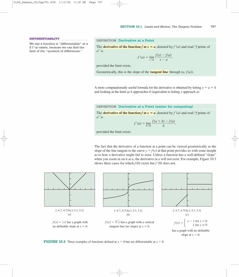
Extending the Ideas57. Graphing the Derivative The graph of f �x� � x2e�x is shown

below. Use your knowledge of the geometric interpretation of thederivative to sketch a rough graph of the derivative y � f �x�.

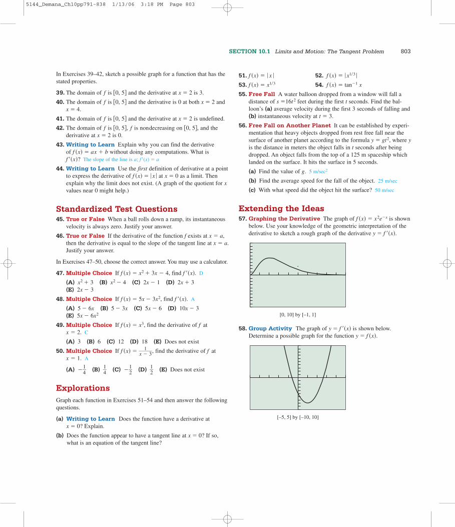
58. Group Activity The graph of y � f �x� is shown below.Determine a possible graph for the function y � f �x�.

[–5, 5] by [–10, 10]

[0, 10] by [–1, 1]




10.2Limits and Motion: The Area Problem

Distance from a Constant Velocity“Distance equals rate times time” is one of the earliest problem-solving formulas thatwe learn in school mathematics. Given a velocity and a time period, we can use the formula to compute distance traveled—as in the following standard example.

EXAMPLE 1 Computing Distance TraveledAn automobile travels at a constant rate of 48 miles per hour for 2 hours and 30 minutes.How far does the automobile travel?

SOLUTION We apply the formula d � rt:

d � �48 mi�hr��2.5 hr� � 120 miles.

The similarity to Example 1 in Section 10.1 is intentional. In fact, if we represent distance traveled (i.e., the change in position) by �s and the time interval by �t, theformula becomes

�s � �48 mph� �t,

which is equivalent to

��

�

st

� � 48 mph.

So the two Example 1s are nearly identical—except that Example 1 of Section 10.1 didnot make an assumption about constant velocity. What we computed in that instancewas the average velocity over the 2.5-hour interval. This suggests that we could haveactually solved the following, slightly different, problem to open this section.

EXAMPLE 2 Computing Distance TraveledAn automobile travels at an average rate of 48 miles per hour for 2 hours and 30 minutes.How far does the automobile travel?

SOLUTION The distance traveled is �s, the time interval has length �t, and �s��tis the average velocity.

Therefore,

�s � ��

�

st

� • �t � �48 mph��2.5 hr� � 120 miles.

So, given average velocity over a time interval, we can easily find distance traveled. Butsuppose we have a velocity function v�t� that gives instantaneous velocity as a changingfunction of time. How can we use the instantaneous velocity function to find distance

Now try Exercise 5.

Now try Exercise 1.

OBJECTIVE

Students will be able to calculate definite integrals using areas.

MOTIVATE

Ask students to guess the meaning of thefollowing statement: lim

x→∞f (x) � 5.

LESSON GUIDE

Day 1: Distance from a Constant Velocity;Distance from a Changing Velocity;Limits at Infinity; The Connection toAreasDay 2: The Definite Integral

What you’ll learn about■ Distance from a Constant

Velocity

■ Distance from a ChangingVelocity

■ Limits at Infinity

■ The Connection to Areas

■ The Definite Integral

. . . and whyLike the tangent line problem,the area problem has manyapplications in every area ofscience, as well as historicaland economic applications.


traveled over a time interval? This was the other intriguing problem about instantaneousvelocity that puzzled the 17th-century scientists—and once again, algebra was inade-quate for solving it, as we shall see.

Distance from a Changing VelocityWhen Galileo began his experiments, here’s what he might have asked himself aboutusing a changing velocity to find distance:

SECTION 10.2 Limits and Motion: The Area Problem 805

One might be tempted to offer the following “solution”:

Velocity times �t gives �s. But instantaneous velocity occurs at an instant of time, so�t � 0. That means �s � 0. So, at any given instant of time, the ball doesn’t move.Since any time interval consists of instants of time, the ball never moves at all! (Youmight well ask: Is this another trick question?)

As was the case with the Velocity Question in Section 10.1, this foolish-looking exam-ple conceals a very subtle algebraic dilemma—and, far from being a trick question, it isexactly the question that needed to be answered in order to compute the distance trav-eled by an object whose velocity varies as a function of time. The scientists who wereworking on the tangent line problem realized that the distance-traveled problem must berelated to it, but, surprisingly, their geometry led them in another direction. The distancetraveled problem led them not to tangent lines, but to areas.

Limits at InfinityBefore we see the connection to areas, let us revisit another limit concept that will makeinstantaneous velocity easier to handle, just as in the last section. We will again be con-tent with an informal definition.

A Distance Question

Suppose a ball rolls down a ramp and its velocity is always 2t feet per second,where t is the number of seconds after it started to roll. How far does the balltravel during the first 3 seconds?

ZENO’S PARADOXES

The Greek philosopher Zeno of Elea(490–425 B.C.) was noted for presentingparadoxes similar to the DistanceQuestion. One of the most famous con-cerns the race between Achilles and aslow-but-sure tortoise. Achilles sportinglygives the tortoise a head start, then setsoff to catch him. He must first gethalfway to the tortoise, but by the timehe runs halfway to where the tortoisewas when he started, the tortoise hasmoved ahead. Now Achilles must closehalf of that distance, but by the time hedoes, the tortoise has moved aheadagain. Continuing this argument forever,we see that Achilles can never evencatch the tortoise, let alone pass him, sothe tortoise must win the race.

DEFINITION (INFORMAL) Limit at Infinity

When we write “limxy

f �x� � L,” we mean that f �x� gets arbitrarily close to L as

x gets arbitrarily large.

EXPLORATION 1 An Infinite Limit

A gallon of water is divided equally and poured into teacups. Find the amountin each teacup and the total amount in all the teacups if there are

1. 10 teacups 0.1 gal; 1 gal

2. 100 teacups 0.01 gal; 1 gal

3. 1 billion teacups 0.000000001 gal; 1 gal

4. an infinite number of teacups 0 gal; 1 gal


Find the number of teacups needed if the amount of water in each teacup is (1) 1 cup, (2) 1 tablespoon, (3) an infi-nitely small amount.(Hint: 1 gallon � 16 cups; 1 cup � 16 tablespoons.)


The preceding Exploration probably went pretty smoothly until you came to the infinitenumber of teacups. At that point you were probably pretty comfortable in saying whatthe total amount would be, and probably a little uncomfortable in saying how muchwould be in each teacup. (Theoretically it would be zero, which is just one reason whythe actual experiment cannot be performed.) In the language of limits, the total amountof water in the infinite number of teacups would look like this:

limny (n • �

1n

� ) � limny

�nn

� � 1 gallon

while the total amount in each teacup would look like this:

limny

�1n

� � 0 gallons.

Summing up an infinite number of nothings to get something is mysterious enoughwhen we use limits; without limits it seems to be an algebraic impossibility. That is thedilemma that faced the 17th-century scientists who were trying to work with instanta-neous velocity. Once again, it was geometry that showed the way when the algebrafailed.

The Connection to AreasIf we graph the constant velocity v � 48 in Example 1 as a function of time t, wenotice that the area of the shaded rectangle is the same as the distance traveled(Figure 10.4). This is no mere coincidence, either, as the area of the rectangle and thedistance traveled over the time interval are both computed by multiplying the sametwo quantities:

�48 mph��2.5 hr� � 120 miles.

Now suppose we graph a velocity function that varies continuously as a function of time(Figure 10.5). Would the area of this irregularly-shaped region still give the total dis-tance traveled over the time interval �a, b�?

Newton and Leibniz (and, actually, many others who had considered this question)were convinced that it obviously would, and that is why they were interested in a cal-culus for finding areas under curves. They imagined the time interval being parti-tioned into many tiny subintervals, each one so small that the velocity over it wouldessentially be constant. Geometrically, this was equivalent to slicing the area into narrow strips, each one of which would be nearly indistinguishable from a narrow rectangle (Figure 10.6).

The idea of partitioning irregularly-shaped areas into approximating rectangles was notnew. Indeed, Archimedes had used that very method to approximate the area of a circlewith remarkable accuracy. However, it was an exercise in patience and perseverance, asExample 3 will show.


FIGURE 10.4 For constant velocity,the area of the rectangle is the same as thedistance traveled, since it represents theproduct of the same two quantities:�48 mph��2.5 hr� � 120 miles.

FIGURE 10.5 If the velocity varies overthe time interval �a, b�, does the shadedregion give the distance traveled?

velocity

batime

Velocity (mph)

48

2.5Time (hr)

velocity

batime

FIGURE 10.6 The region is partitionedinto vertical strips. If the strips are narrowenough, they are almost indistinguishablefrom rectangles. The sum of the areas of these “rectangles” will give the total area and can be interpreted as distance traveled.


EXAMPLE 3 Approximating an Area with Rectangles

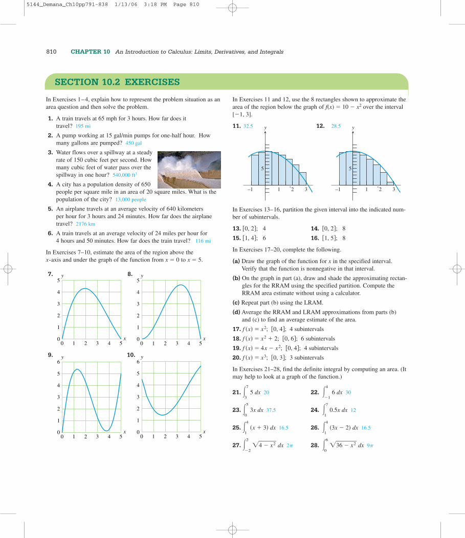
Use the six rectangles in Figure 10.7 to approximate the area of the region below thegraph of f �x� � x2 over the interval �0, 3�.

SOLUTION The base of each approximating rectangle is 1�2. The height is deter-mined by the function value at the right-hand endpoint of each subinterval. The areasof the six rectangles and the total area are computed in the table below:

Base of Height of Area of Subinterval rectangle rectangle rectangle

�0, 1�2� 1�2 f �1�2�¬� �1�2�2 � 1�4 �1/2��1/4�¬� 0.125

�1�2, 1� 1�2 f �1�¬� �1�2 � 1 �1�2��1�¬� 0.500

�1, 3�2� 1�2 f �3�2�¬� �3�2�2 � 9�4 �1�2��9�4�¬� 1.125

�3�2, 2� 1�2 f �2�¬� �2�2 � 4 �1�2��4�¬� 2.000

�2, 5�2� 1�2 f �5�2�¬� �5�2�2 � 25�4 �1�2��25�4�¬� 3.125

�5�2, 3� 1�2 f �3�¬� �3�2 � 9 �1�2��9�¬� 4.500

Total Area: 11.375

The six rectangles give a (rather crude) approximation of 11.375 square units for thearea under the curve from 0 to 3.

Figure 10.7 shows that the right rectangular approximation method (RRAM) in Example 4overestimates the true area. If we were to use the function values at the left-hand end-points of the subintervals (LRAM), we would obtain a rectangular approximation(6.875 square units) that underestimates the true area (Figure 10.8). The average of thetwo approximations is 9.125 square units, which is actually a pretty good estimate ofthe true area of 9 square units. If we were to repeat the process with 20 rectangles, theaverage would be 9.01125. This method of converging toward an unknown area byrefining approximations is tedious, but it works—Archimedes used a variation of it2200 years ago to estimate the area of a circle, and in the process demonstrated that theratio of the circumference to the diameter was between 3.140845 and 3.142857.

The calculus step is to move from a finite number of rectangles (yielding an approxi-mate area) to an infinite number of rectangles (yielding an exact area). This brings us tothe definite integral.



FIGURE 10.7 The area under the graph of f (x) � x2 is approximated by six rec-tangles, each with base 1�2. The height ofeach rectangle is the function value at the right-hand endpoint of the subinterval(Example 3).

5

y

10

x2 31

FIGURE 10.8 If we change the rectanglesin Figure 10.7 so that their heights are deter-mined by function values at the left-handendpoints, we get an area approximation(6.875 square units) that underestimates thetrue area.

5

y

10

x2 31


The Definite IntegralIn general, begin with a continuous function y � f �x� over an interval �a, b�. Divide�a, b� into n subintervals of length �x � �b � a��n. Choose any value x1 in the firstsubinterval, x2 in the second, and so on. Compute f �x1�, f �x2�, f �x3�, …, f �xn�, multi-ply each value by �x, and sum up the products. In sigma notation, the sum of theproducts is

�n

i�1f �xi��x.

The limit of this sum as n approaches infinity is the solution to the area problem, andhence the solution to the problem of distance traveled. Indeed, it solves a variety ofother problems as well, as you will learn when you study calculus. The limit, if it exists,is called a definite integral.


RIEMANN SUMS

A sum of the form �n

i�1f(xi)�x in which x1

is in the first subinterval, x2 is in the sec-ond, and so on, is called a Riemann sum,in honor of Georg Riemann (1826–1866),who determined the functions for whichsuch sums had limits as n→∞.

DEFINITE INTEGRAL NOTATION

Notice that the notation for the definiteintegral (another legacy of Leibniz) parallels the sigma notation of the sumfor which it is a limit. The “�” in the limitbecomes a stylized “S,” for “sum.” The“�x” becomes “dx” (as it did in thederivative), and the “f(xi)” becomes sim-ply “f(x)” because we are effectively summing up all the f(x) values along the interval (times an arbitrarily smallchange in x), rendering the subscriptsunnecessary.

DEFINITION Definite Integral

Let f be a function defined on �a, b� and let �n

i�1f �xi��x be defined as above. The

definite integral of f over �a, b�, denoted �b

af �x� dx, is given by

�b

af �x�dx � lim

n→ �n

i�1f �xi��x,

provided the limit exists. If the limit exists, we say f is on �a, b�.integrable

The solution to Example 4 shows that it can be tedious to approximate a definite inte-gral by working out the sum for a large value of n. One of the crowning achievementsof calculus was to demonstrate how the exact value of a definite integral could beobtained without summing up any products at all. You will have to wait until calculus tosee how that is done; meanwhile, you will learn in Section 10.4 how to use a calculatorto take the tedium out of finding definite integrals by summing.

You can also use the area connection to your advantage, as shown in these next twoexamples.

EXAMPLE 4 Computing an Integral

Find �5

12x dx.

SOLUTION This will be the area under the line y � 2x over the interval �1, 5�. Thegraph in Figure 10.9 shows that this is the area of a trapezoid.

Using the formula A � h(�b1 �

2b2� ), we find that

�5

12x dx � 4(�2(1) �

22(5)

� ) � 24


y

x1 5

y = 2x

FIGURE 10.9 The area of the trapezoid

equals �5

12x dx. (Example 4)


EXAMPLE 5 Computing an IntegralSuppose a ball rolls down a ramp so that its velocity after t seconds is always 2t feetper second. How far does it fall during the first 3 seconds?

SOLUTION The distance traveled will be the same as the area under the velocitygraph, v �t� � 2t, over the interval �0, 3�. The graph is shown in Figure 10.10. Sincethe region is triangular, we can find its area: A � �1�2��3��6� � 9. The distance traveled in the first 3 seconds, therefore, is �s � �1�2��3 sec��6 feet�sec� � 9 feet.



FIGURE 10.10 The area under the velocity graph v�t� � 2t, over the interval �0, 3� is thedistance traveled by the ball in Example 5 during the first 3 seconds.

6

v

t1 2 3

FOLLOW-UP

Ask students to explain why the RRAMapproximation for the area under a curvebecomes more accurate as the number ofrectangles, n, increases.

ASSIGNMENT GUIDE

Day 1: Ex. 1–19 odd, 47–50Day 2: Ex. 21–45, multiples of 3, 59, 62

COOPERATIVE ACTIVITY

Group Activity: Ex. 57, 59–64

NOTES ON EXERCISES

Ex. 21–38 are designed to help studentsunderstand the connection between thedefinite integral and areas.Ex. 49–50 require students to estimateareas using data.Ex. 51–56 provide practice with standard-ized tests.Ex. 59–64 introduce students to some ofthe properties of definite integrals.

ONGOING ASSESSMENT

Self-Assessment: Ex. 1, 5, 11, 23, 45Embedded Assessment: Ex. 43–44, 58

QUICK REVIEW 10.2 (For help, go to Sections 1.1 and 9.4.)

In Exercises 1 and 2, list the elements of the sequence.

1. ak � �12

� ( �12

� k )2

for k � 1, 2, 3, 4, . . . , 9, 10

2. ak � �14

� (2 � �14

� k )2

for k � 1, 2, 3, 4, . . . , 9, 10

In Exercises 3–6, find the sum.

3. �10

k�1�12

� �k � 1� �625� 4. �

n

k�1�k � 1� �

n(n2� 3)�

5. �10

k�1�12

� �k � 1�2 �5025

� 6. �n

k�1�12

� k2 �n(n � 1

1)(22n � 1)�

7. A truck travels at an average speed of 57 mph for 4 hours.How far does it travel? 228 miles

8. A pump working at 5 gal/min pumps for 2 hours. How manygallons are pumped? 600 gal

9. Water flows over a spillway at a steady rate of 200 cubic feetper second. How many cubic feet of water pass over thespillway in 6 hours? 4,320,000 ft3

10. A county has a population density of 560 people per squaremile in an area of 35,000 square miles. What is the popula-tion of the county? 19,600,000 people




In Exercises 1–4, explain how to represent the problem situation as anarea question and then solve the problem.

1. A train travels at 65 mph for 3 hours. How far does it travel? 195 mi

2. A pump working at 15 gal/min pumps for one-half hour. Howmany gallons are pumped? 450 gal

3. Water flows over a spillway at a steadyrate of 150 cubic feet per second. Howmany cubic feet of water pass over thespillway in one hour? 540,000 ft3

4. A city has a population density of 650people per square mile in an area of 20 square miles. What is thepopulation of the city? 13,000 people

5. An airplane travels at an average velocity of 640 kilometers per hour for 3 hours and 24 minutes. How far does the airplanetravel? 2176 km

6. A train travels at an average velocity of 24 miles per hour for 4 hours and 50 minutes. How far does the train travel? 116 mi

In Exercises 7–10, estimate the area of the region above the x-axis and under the graph of the function from x � 0 to x � 5.

7. 8.

9. 10.

x

y

00

1

2

3

4

5

6

1 2 3 4 5x

y

00

1

2

3

4

5

6

1 2 3 4 5

x

y

00

1

2

3

4

5

1 2 3 4 5x

y

00

1

2

3

4

5

1 2 3 4 5

In Exercises 11 and 12, use the 8 rectangles shown to approximate thearea of the region below the graph of f(x) � 10 � x2 over the interval[�1, 3].

11. 12.

In Exercises 13–16, partition the given interval into the indicated num-ber of subintervals.

13. �0, 2�; 4 14. �0, 2�; 815. �1, 4�; 6 16. �1, 5�; 8

In Exercises 17–20, complete the following.

(a) Draw the graph of the function for x in the specified interval.Verify that the function is nonnegative in that interval.

(b) On the graph in part (a), draw and shade the approximating rectan-gles for the RRAM using the specified partition. Compute theRRAM area estimate without using a calculator.

(c) Repeat part (b) using the LRAM.

(d) Average the RRAM and LRAM approximations from parts (b) and (c) to find an average estimate of the area.

17. f �x� � x2; �0, 4�; 4 subintervals

18. f �x� � x2 � 2; �0, 6�; 6 subintervals

19. f �x� � 4x � x2; �0, 4�; 4 subintervals

20. f �x� � x3; �0, 3�; 3 subintervals

In Exercises 21–28, find the definite integral by computing an area. (Itmay help to look at a graph of the function.)

21. �7

35 dx 20 22. �4

�16 dx 30

23. �5

03x dx 37.5 24. �7

10.5x dx 12

25. �4

1�x � 3� dx 16.5 26. �4

1�3x � 2� dx 16.5

27. �2

�2�4� �� x�2� dx 2� 28. �6

0�3�6� �� x�2� dx 9�

5

y

2 31–1

5

y

2 31–1

32.5 28.5


It can be shown that the area enclosed between the x-axis and one archof the sine curve is 2. Use this fact in Exercises 29–38 to compute thedefinite integral. (It may help to look at a graph of the function.)

29. ��

0sin x dx 2 30. ��

0�sin x � 2� dx 2 � 2�

31. ��2

2sin �x � 2� dx 2 32. ��/2

��/2cos x dx 2

33. ��/2

0sin x dx 1 34. ��/2

0cos x dx 1

35. ��

02 sin x dx [Hint: All the rectangles are twice as tall.] 4

36. �2�

0sin ( �

2x

� ) dx [Hint: All the rectangles are twice as wide.]

37. �2�

0�sin x � dx 4 38. �3�/2

��

�cos x � dx 5

In Exercises 39–42, find the integral assuming that k is a numberbetween 0 and 4.

39. �4

0(kx � 3) dx 8k � 12 40. �k

0(4x � 3) dx 2k2 � 3k

41. �4

0(3x � k) dx 24 � 4k 42. �4

k(4x � 3) dx

43. Writing to Learn Let g�x� � � f �x� where f has nonnegativefunction values on an interval �a, b�. Explain why the area abovethe graph of g is the same as the area under the graph of f in thesame interval.

44. Writing to Learn Explain how you can find the area underthe graph of f �x� � �1�6� �� x�2� from x � 0 to x � 4 by mental com-putation only.

45. Falling Ball Suppose a ball is dropped from a tower and itsvelocity after t seconds is always 32t feet per second. How far doesthe ball fall during the first 2 seconds? 64 ft

46. Accelerating Automobile Suppose an automobile acceleratesso that its velocity after t seconds is always 6t feet per second.How far does the car travel in the first 7 seconds? 147 ft

47. Rock Toss A rock is thrown straight up from level ground. Thevelocity of the rock at any time t (sec) is v�t� � 48 � 32t ft�sec.

(a) Graph the velocity function.

(b) At what time does the rock reach its maximum height?

(c) Find how far the rock has traveled at its maximum height.

48. Rocket Launch A toy rocket is launched straight up from levelground. Its velocity function is f �t� � 170 � 32t feet per second,where t is the number of seconds after launch.

(a) Graph the velocity function.

(b) At what time does the rocket reach its maximum height?

(c) Find how far the rocket has traveled at its maximum height. 451.6 ft

49. Finding Distance Traveled as Area A ball is pushed off theroof of a three-story building. Table 10.3 gives the velocity (in feetper second) of the falling ball at 0.2-second intervals until it hitsthe ground 1.4 seconds later.

(a) Draw a scatter plot of the data.

(b) Find the approximate building height using RRAM areas as inExample 4. Use the fact that if the velocity function is alwaysnegative the distance traveled will be the same as if the absolutevalue of the velocity values were used. 33.86 ft

50. Work Work is defined as force times distance. A full water barrelweighing 1250 pounds has a significant leak and must be lifted 35 feet. Table 10.4 displays the weight of the barrel measured after each 5 feet of movement. Find the approximate work in foot-pounds done in lifting the barrel 35 feet. 31,500 ft-pounds

Standardized Test Questions51. True or False When estimating the area under a curve using

LRAM, the accuracy typically improves as the number n of subin-tervals is increased.

52. True or False The statement limx→

f �x� � L means that

f �x� gets arbitrarily large as x gets arbitrarily close to L.

Table 10.4 Weight of a Leaking Water Barrel

Distance (ft) Weight (lb)

0 12505 1150

10 105015 95020 85025 75030 650

Table 10.3 Velocity Data of the Ball

Time Velocity

0.2 �5.050.4 �11.430.6 �17.460.8 �24.211.0 �30.621.2 �37.061.4 �43.47



It can be shown that the area of the region enclosed by the curve y � �x�, the x-axis, and the line x � 9 is 18. Use this fact inExercises 53–56 to choose the correct answer. Do not use a calculator.

53. Multiple Choice �0

9

2�x� dx A

(A) 36 (B) 27 (C) 18 (D) 9 (E) 6


9

�x� � 5� dx E

(A) 14 (B) 23 (C) 33 (D) 45 (E) 63


14

�x � 5�� dx C

(A) 9 (B) 13 (C) 18 (D) 23 (E) 28


3

�3�x dx D

(A) 54 (B) 18 (C) 9 (D) 6 (E) 3

Explorations57. Group Activity You may have erroneously assumed that the

function f had to be positive in the definition of the definite

integral. It is a fact that �2�

0sin x dx � 0. Use the definition of

the definite integral to explain why this is so. What does this imply

about �1

0�x � 1� dx?

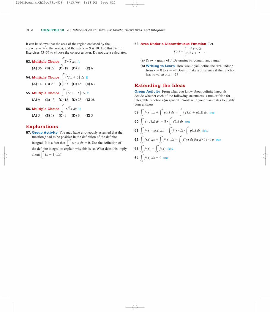
58. Area Under a Discontinuous Function Let

f �x� � .

(a) Draw a graph of f. Determine its domain and range.

(b) Writing to Learn How would you define the area under ffrom x � 0 to x � 4? Does it make a difference if the functionhas no value at x � 2?

Extending the IdeasGroup Activity From what you know about definite integrals,decide whether each of the following statements is true or false forintegrable functions (in general). Work with your classmates to justifyyour answers.

59. �b

af �x� dx � �b

ag�x� dx � �b

a� f �x� � g�x�� dx true

60. �b

a8 • f �x� dx � 8 • �b

af �x� dx true

61. �b

af �x� • g�x� dx � �b

af �x� dx • �b

ag�x� dx false

62. �c

af �x� dx � �b

cf �x� dx � �b

af �x� dx for a c b true

63. �b

af �x� � �a

bf �x� false

64. �a

af �x� dx � 0 true

1 if x 2x if x � 2



SECTION 10.3 More on Limits 813

10.3More on Limits

A Little HistoryProgress in mathematics occurs gradually and without much fanfare in the earlystages. The fanfare occurs much later, after the discoveries and innovations have beencleaned up and put into perspective. Calculus is certainly a case in point. Most of theideas in this chapter pre-date Newton and Leibniz. Others were solving calculusproblems as far back as Archimedes of Syracuse (ca. 287–212 B.C.), long before cal-culus was “discovered.” What Newton and Leibniz did was to develop the rules ofthe game, so that derivatives and integrals could be computed algebraically. Mostimportantly, they developed what has come to be called the Fundamental Theorem ofCalculus, which explains the connection between the “tangent line problem” and the“area problem.”

But the methods of Newton and Leibniz depended on mysterious “infinitesimal” quan-tities that were small enough to vanish and yet were not zero. Jean Le Rond d’Alembert(1717–1783) was a strong proponent of replacing infinitesimals with limits (the strat-egy that would eventually work), but these concepts were not well understood untilKarl Weierstrass (1815–1897) and his student Eduard Heine (1821–1881) introducedthe formal, unassailable definitions that are used in our higher mathematics coursestoday. By that time, Newton and Leibniz had been dead for over 150 years.

Defining a Limit InformallyThere is nothing difficult about the following limit statements:

limx→3

(2x � 1) � 5 limx→

�x2 � 3� � limn→

�1n

� � 0

That is why we have used limit notation throughout this book. Particularly when elec-tronic graphers are available, analyzing the limiting behavior of functions alge-braically, numerically, and graphically can tell us much of what we need to knowabout the functions.

What is difficult is to come up with an air-tight definition of what a limit really is. If ithad been easy, it would not have taken 150 years. The subtleties of the “epsilon-delta”definition of Weierstrass and Heine are as beautiful as they are profound, but they arenot the stuff of a precalculus course. Therefore, even as we look more closely at limitsand their properties in this section, we will continue to refer to our “informal” defini-tion of limit (essentially that of d’Alembert). We repeat it here for ready reference:

OBJECTIVE

Students will be able to use the propertiesof limits and evaluate one-sided limits,two-sided limits, and limits involvinginfinity.

MOTIVATE

Discuss whether limx→2

int (x) exists, where

int x represents the greatest integer that isless than or equal to x.

LESSON GUIDE

Day 1: A Little History; Defining a LimitInformally; Properties of Limits; Limitsof Continuous Functions; One-Sided andTwo-Sided LimitsDay 2: Limits Involving Infinity

TEACHING NOTE

For reference, the formal “epsilon-delta”definition of a limit is given below. Notethat “f(x) gets arbitrarily close to L”means f(x) is within � units of L, and “x gets arbitrarily close to a” means x is within � units of a. f(x) has a limit Las x approaches a (that is, lim

x→af(x) � L)

if and only if for any � � 0 there exists anumber � � 0 such that, whenever �x � a � �, we have � f(x) � L � �.

DEFINITION (INFORMAL) Limit at a

When we write “limxya

f �x� � L,” we mean that f �x� gets arbitrarily close to L as x

gets arbitrarily close (but not equal) to a.

What you’ll learn about■ A Little History

■ Defining a Limit Informally

■ Properties of Limits

■ Limits of ContinuousFunctions

■ One-Sided and Two-SidedLimits

■ Limits Involving Infinity

. . . and whyLimits are essential concepts inthe development of calculus.



EXPLORATION 1 What’s the Limit?

As a class, discuss the following two limit statements until you really under-stand why they are true. Look at them every way you can. Use your calculators.Do you see how the above definition verifies that they are true? In particular,can you defend your position against the challenges that follow the statements?(This exploration is intended to be free-wheeling and philosophical. You can’tprove these statements without a stronger definition.)

1. limx→2

7x � 14.000000000000000001

Challenges:

• Isn’t 7x getting “arbitrarily close” to that number as x approaches 2?

• How can you tell that 14 is the limit and 14.000000000000000001 is not?

2. limx→0

�x2 �

x2x

� � 2

Challenges:

• How can the limit be 2 when the quotient isn’t even defined at 0?

• Won’t there be an asymptote at x � 0? The denominator equals 0there.

• How can you tell that 2 is the limit and 1.99999999999999999999 is not?

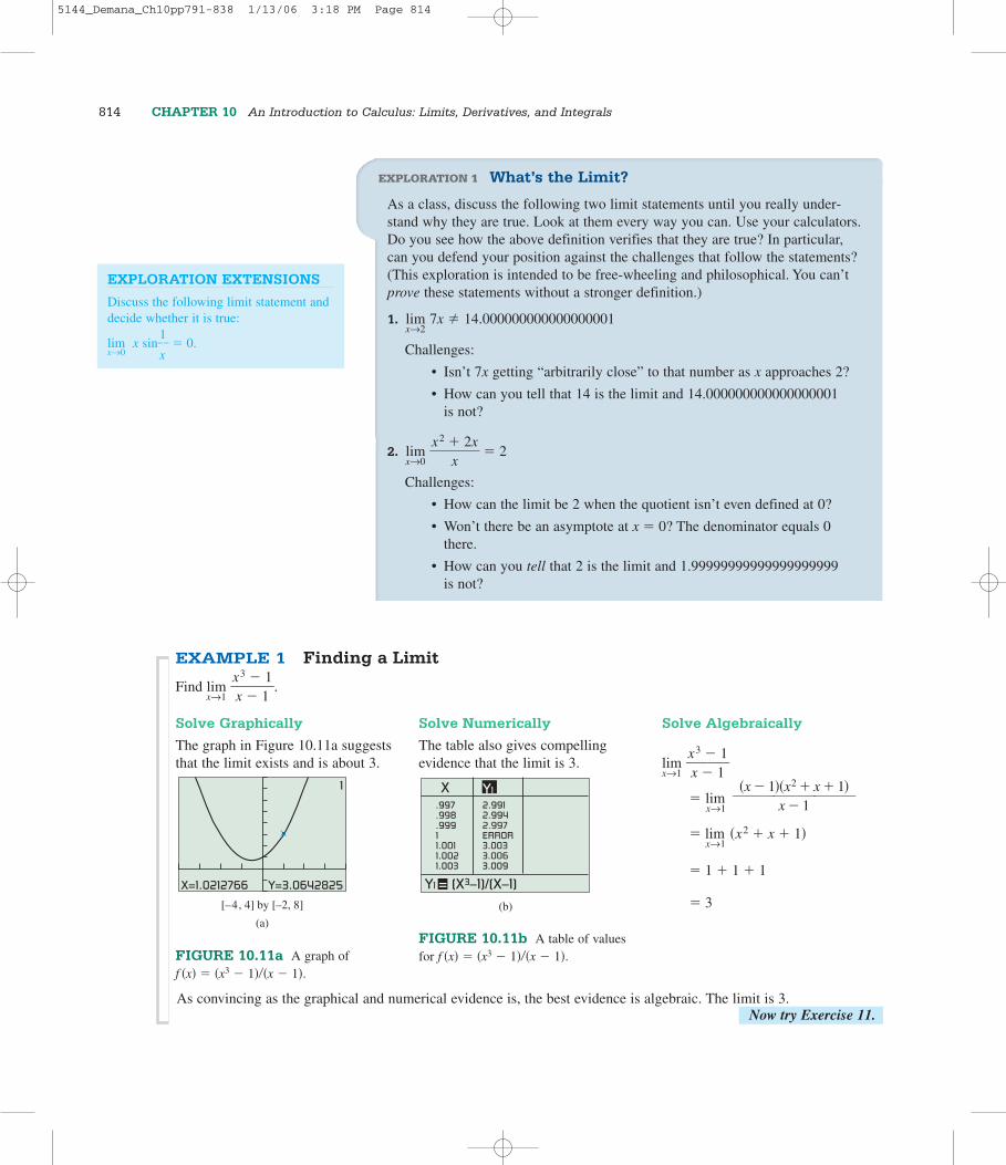
Solve Graphically

The graph in Figure 10.11a suggeststhat the limit exists and is about 3.

FIGURE 10.11a A graph of f �x� � �x3 � 1��x � 1�.

Solve Numerically

The table also gives compelling evidence that the limit is 3.

FIGURE 10.11b A table of valuesfor f �x� � �x3 � 1��x � 1�.

Solve Algebraically

limx→1

�xx

3

�

�

11

�

� limx→1

¬ � limx→1

�x2 � x � 1�

� 1 � 1 � 1

� 3

�x � 1��x2 � x � 1��

x � 1X

Y1 = (X3–1)/(X–1)

.997

.998

.99911.0011.0021.003

2.9912.9942.997ERROR3.0033.0063.009

Y1

(b)[–4, 4] by [–2, 8]

(a)

X=1.0212766 Y=3.0642825

1

EXAMPLE 1 Finding a Limit

Find limx→1

�xx

3

�

�

11

�.

As convincing as the graphical and numerical evidence is, the best evidence is algebraic. The limit is 3.


Discuss the following limit statement anddecide whether it is true:

limx→0

x sin�x

1� � 0.



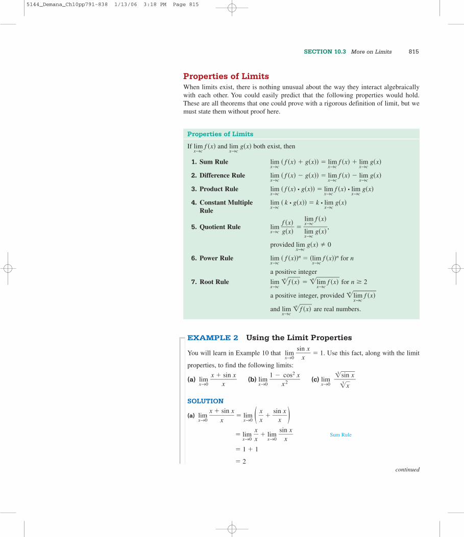
Properties of LimitsWhen limits exist, there is nothing unusual about the way they interact algebraicallywith each other. You could easily predict that the following properties would hold.These are all theorems that one could prove with a rigorous definition of limit, but wemust state them without proof here.


Properties of Limits

If limx→c

f �x� and limx→c

g�x� both exist, then

1. Sum Rule limx→c

� f �x� � g�x�� limx→c

f �x� � limx→c

g�x�

2. Difference Rule limx→c

� f �x� � g�x�� limx→c

f �x� � limx→c

g�x�

3. Product Rule limx→c

� f �x� • g�x�� limx→c

f �x� • limx→c

g�x�

4. Constant Multiple limx→c

� k • g�x�� k • limx→c

g�x�Rule

5. Quotient Rule limx→c

�gf ��xx��

� � �l

l

i

i

mx→

mx→

c

c

g

f �

�

x

x

�

��,

provided limx→c

g�x� � 0

6. Power Rule limx→c

� f �x��n � �limx→c

f �x��n for n

a positive integer

7. Root Rule limx→c

�nf ��x�� n li�m

x→c�f ��x�� for n � 2

a positive integer, provided �n li�mx→c

�f ��x��

and limx→c

�nf ��x�� are real numbers.

EXAMPLE 2 Using the Limit Properties

You will learn in Example 10 that limx→0

�sin

xx

� � 1. Use this fact, along with the limit

properties, to find the following limits:

(a) limx→0

�x �

xsin x� (b) lim

x→0�1 �

xc2os2 x� (c) lim

x→0��3

�

s3

in

x�

x��

SOLUTION

(a) limx→0

�x �

x

sin x�¬� lim

x→0 ( �xx

� � �sin

xx

� )� lim

x→0�xx

� � limx→0

�sin

xx

� Sum Rule

¬ � 1 � 1

¬ � 2continued


(b) limx→0

�1 �

xc2os2 x� � lim

x→0�si

xn

2

2 x� Pythagorean identity

� limx→0 (�

sinx

x� )(�

sinx

x� )

� limx→0 (�

sinx

x� ) • lim

x→0 (�sin

xx

� ) Product Rule

� 1 • 1

� 1

(c) limx→0

��3

�s3

i�n�x�

x�� lim

x→0 �3 �s�in

x� x��

� �3 li�mx→0��

s�inx� x�� Root Rule

� �3 1�

� 1

Limits of Continuous FunctionsRecall from Section 1.2 that a function is continuous at a if lim

x→af �x� � f �a�. This means

that the limit (at a) of a function can be found by “plugging in a” provided the function iscontinuous at a. (The condition of continuity is essential when employing this strategy. Forexample, plugging in 0 does not work on any of the limits in Example 2.)

EXAMPLE 3 Finding Limits by SubstitutionFind the limits.

(a) limx→0

�ex

c�

ost2axn x

� (b) limn→16

�lo�g2

n�n

�

SOLUTION

You might not recognize these functions as being continuous, but you can use the limitproperties to write the limits in terms of limits of basic functions.

(a) limx→0

�ex

c�

ost2axn x

� � Quotient Rule

� Difference and Power Rules

� �e0

�c�

osta0n�2

0� Limits of continuous functions

� �1 �

10

�

� 1

limx→0

ex � limx→0

tan x��

�limx→0

cos x�2

limx→0

�ex � tan x��

limx→0

�cos2 x�



continued


(b) limn→16

�lo�g2

n�n

� � Quotient Rule

� �lo�g2

1�16�6

� Limits of continuous functions

� �44

�

� 1

Example 3 hints at some important properties of continuous functions that follow fromthe properties of limits. If f and g are both continuous at x � a, then so are f � g, f – g,fg, and f�g (with the assumption that g(a) does not create a zero denominator in the quo-tient). Also, the nth power and nth root of a function that is continuous at a will also becontinuous at a (with the assumption that �f (a)� is real).

One-sided and Two-sided LimitsWe can see that the limit of the function in Figure 10.11 is 3 whether x approaches 1 fromthe left or right. Sometimes the values of a function f can approach different values as x approaches a number c from opposite sides. When this happens, the limit of f as x approaches c from the left is the of f at c and the limit of f as xapproaches c from the right is the of f at c. Here is the notation we use:

left-hand: limxyc�

f �x� The limit of f as x approaches c from the left.

right-hand: limxyc�

f �x� The limit of f as x approaches c from the right.

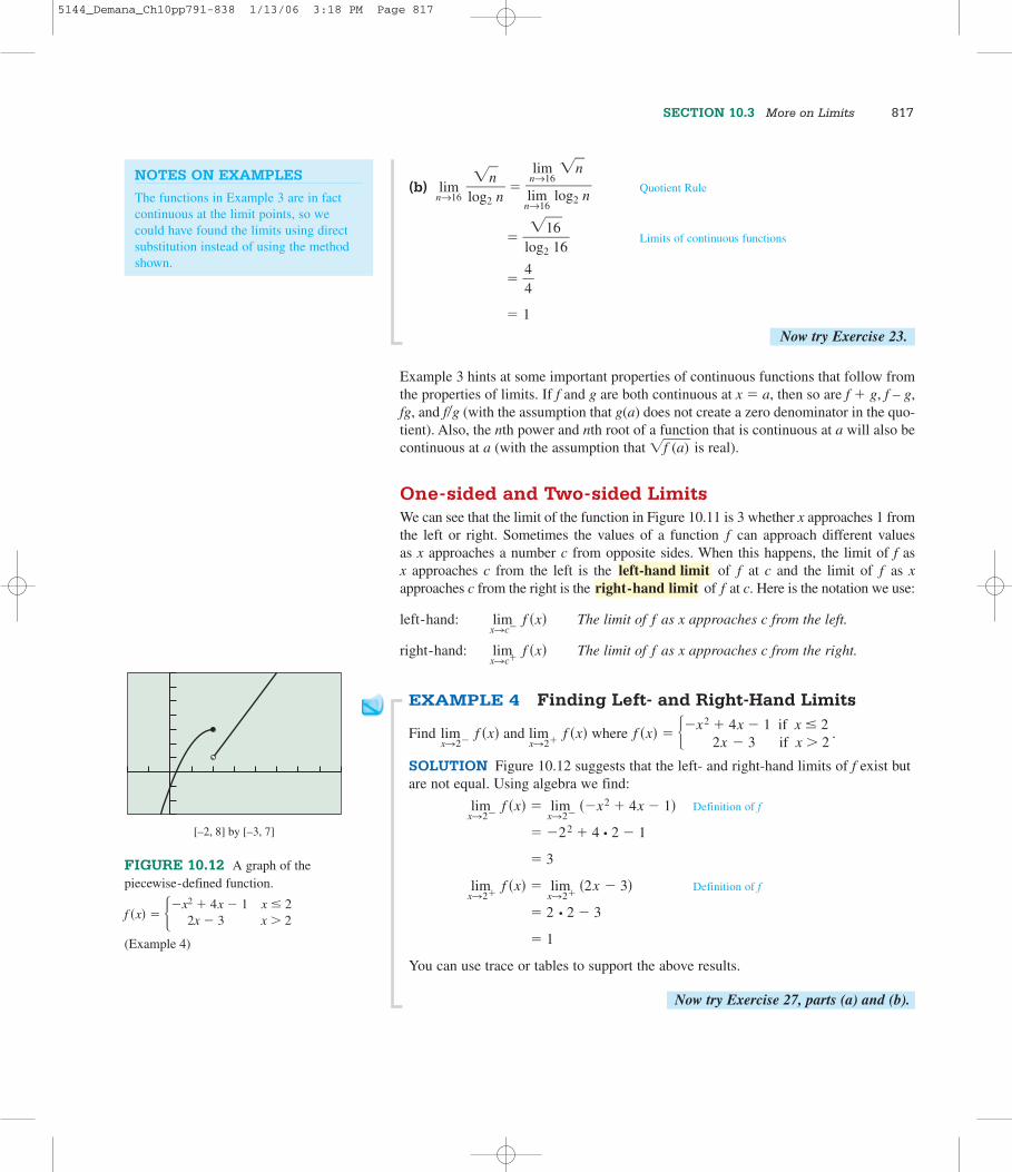
EXAMPLE 4 Finding Left- and Right-Hand Limits

Find limxy2�

f �x� and limxy2�

f �x� where f �x� � .

SOLUTION Figure 10.12 suggests that the left- and right-hand limits of f exist butare not equal. Using algebra we find:

limxy2�

f �x� � limxy2�

��x2 � 4x � 1� Definition of f

� �22 � 4 • 2 � 1

� 3

limxy2�


�2x � 3� Definition of f

� 2 • 2 � 3

� 1

You can use trace or tables to support the above results.

Now try Exercise 27, parts (a) and (b).

�x2 � 4x � 1 if x � 22x � 3 if x � 2

right-hand limitleft-hand limit


limn→16

�n��lim

n→16log2 n


FIGURE 10.12 A graph of thepiecewise-defined function.

f �x� � (Example 4)

�x2 � 4x � 1 x � 22x � 3 x � 2

[–2, 8] by [–3, 7]

NOTES ON EXAMPLES

The functions in Example 3 are in factcontinuous at the limit points, so wecould have found the limits using directsubstitution instead of using the methodshown.


The limit limxyc

f �x� is sometimes called the of f at c to distinguish itfrom the one-sided left-hand and right-hand limits of f at c. The following theoremindicates how these limits are related.

two-sided limit


The limit of the function f of Example 4 as x approaches 2 does not exist, so f is dis-continuous at x � 2. However, discontinuous functions can have a limit at a point ofdiscontinuity. The function f of Example 1 is discontinuous at x � 1 because f �1� doesnot exist, but it has the limit 3 as x approaches 1. Example 5 illustrates another way afunction can have a limit and still be discontinuous.

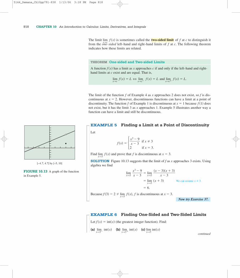
EXAMPLE 5 Finding a Limit at a Point of Discontinuity

Let

f �x� � Find lim

xy3f �x� and prove that f is discontinuous at x � 3.

SOLUTION Figure 10.13 suggests that the limit of f as x approaches 3 exists. Usingalgebra we find

limxy3

�xx

2

�

�

39

� � limxy3

��x �

x3�

��x3� 3�

�

� limxy3

�x � 3� We can assume x � 3.

� 6.

Because f �3� � 2 � limxy3

f �x�, f is discontinuous at x � 3.

EXAMPLE 6 Finding One-Sided and Two-Sided Limits

Let f �x� � int�x� (the greatest integer function). Find:

(a) limxy3�

int�x� (b) limxy3�

int�x� (c) limxy3

int�x�


�xx

2

�

�

39

� if x � 3

2 if x � 3.

THEOREM One-sided and Two-sided Limits

A function f �x� has a limit as x approaches c if and only if the left-hand and right-hand limits at c exist and are equal. That is,

limxyc

f �x� � L ⇔ limxyc�

f �x� � L and limxyc�

f �x� � L.

FIGURE 10.13 A graph of the functionin Example 5.

[–4.7, 4.7] by [–5, 10]

continued


SOLUTION Recall that int �x� is equal to the greatest integer less than or equal to x.For example, int�3� � 3. From the definition of f and its graph in Figure 10.14 we cansee that

(a) limxy3�

int�x� � 2

(b) limxy3�

int�x� � 3

(c) limxy3

int�x� does not exist.

Limits Involving InfinityThe informal definition that we have for a limit refers to lim

xyaf �x� � L where both a and

L are real numbers. In Section 10.2 we adapted the definition to apply to limits of the form lim

xy f �x� � L so that we could use this notation in describing definite integrals.

This is one type of “limit at infinity.” Notice that the limit itself �L� is a finite real num-ber, assuming the limit exists, but that the values of x are approaching infinity.



Notice that limits, whether at a or at infinity, are always finite real numbers; otherwise,the limits do not exist. For example, it is correct to write

limx→0

�x12� does not exist,

since it approaches no real number L. In this case, however, it is also convenient to write

limx→0

�x12� � ,

which gives us a little more information about why the limit fails to exist. (It increaseswithout bound.) Similarly, it is convenient to write

limx→0�

ln x � � ,

since ln x decreases without bound as x approaches 0 from the right. In this context, thesymbols “ ” and “� ” are sometimes called .infinite limits

INFINITE LIMITS ARE NOT LIMITS

It is important to realize that an infinitelimit is not a limit, despite what thename might imply. It describes a specialcase of a limit that does not exist. Recallthat a sawhorse is not a horse and a bad-minton bird is not a bird.

ARCHIMEDES (CA. 287–212 B.C.)

The Greek mathematician Archimedesfound the area of a circle using a methodinvolving infinite limits. See Exercise 89for a modern version of his method.

NOTES ON EXAMPLES

Examples 5 and 6 demonstrate that it isnot necessarily true that lim

x→cf (x) � f (c).

Make certain that students understand therole of continuity in evaluating limits.

FIGURE 10.14 The graph of f(x) � int(x). (Example 6)

[–5, 5] by [–5, 5]

DEFINITION Limits at Infinity

When we write “limxy

f �x� � L,” we mean that f �x� gets arbitrarily close to L as x

gets arbitrarily large. We say that f has a limit L as x approaches �.

When we write “limx→�

f �x� � L,” we mean that f �x� gets arbitrarily close to L as �x

gets arbitrarily large. We say that f has a limit L as x approaches ��.


EXAMPLE 7 Investigating Limits as xy��

Let f �x� � �sin x��x. Find limxy

f �x� and limxy�

f �x�.

SOLUTION The graph of f in Figure 10.15 suggests that

limxy

�sin

xx

� � limxy�

�sin

xx

� � 0.

In Section 1.3, we used limits to describe the unbounded behavior of the functionf �x� � x3 as xy � :

limxy

x3 � and limxy�

x3 � �

The behavior of the function g�x� � ex as x y � can be described by the followingtwo limits:

limxy

ex � and limxy�

ex � 0

The function g�x� � ex has unbounded behavior as x y and has a finite limit asxy � .

EXAMPLE 8 Using Tables to Investigate Limits as xy��

Let f �x� � xe�x. Find limxy


f �x�.

SOLUTION The tables in Figure 10.16 suggest that

limxy

xe�x � 0 and limxy�

xe�x � � .

FIGURE 10.16 The table in (a) suggests that the values of f (x) � xe�x approach 0 asxy and the table in (b) suggests that the values of f (x) � xe�x approach � as xy � .(Example 8)

The graph of f in Figure 10.17 supports these results.Now try Exercise 49.

X

Y2 = Xe^(–X)

0–10–20–30–40–50–60

0–2.2E5–9.7E9–3E14–9E18–3E23–7E27

Y2

(b)

X

Y2 = Xe^(–X)

0102030405060

04.5E–44.1E–83E–122E–161E–205E–25

Y2

(a)



FIGURE 10.15 The graph of f (x) � (sin x)�x. (Example 7)

[–20, 20] by [–2, 2]

FIGURE 10.17 The graph of thefunction f (x) � xe�x. (Example 8)

[–5, 5] by [–5, 5]

FOLLOW-UP

Ask students to discuss the followingstatement and determine for what valuesof k and c it is true: lim

x→ckx � kc.

ASSIGNMENT GUIDE

Day 1: Ex. 3–39, multiples of 3Day 2: Ex. 42–87, multiples of 3


Group Activity: Ex. 35–36, 84–87

NOTES ON EXERCISES

Ex. 1–60 are basic exercises involvingleft-hand, right-hand, and two-sided limits.Ex. 73–78 provide practice with standard-ized tests.Ex. 84–87 give students an opportunity tocreate functions with specified properties.

ONGOING ASSESSMENT

Self-Assessment: Ex. 11, 19, 23, 27, 37,41, 47, 49, 51, 55, 63, 65, 67Embedded Assessment: Ex. 37–40


In Section 2.6 we used the graph of f �x� � 1��x � 2� to state that

limxy2�

�x �

12

� � � and limxy2�

�x �

12

� � .

Either one of these unbounded limits allows us to conclude that the vertical line x � 2is a vertical asymptote of the graph of f (Figure 10.18).

EXAMPLE 9 Investigating Unbounded LimitsFind lim

xy21��x � 2�2.

SOLUTION The graph of f �x� � 1��x � 2�2 in Figure 10.19 suggests that

limxy2�

��x �

12�2� � and lim

xy2��x �

12�2� � .

This means that the limit of f as x approaches 2 does not exist. The table of values inFigure 10.20 agrees with this conclusion. The graph of f has a vertical asymptote atx � 2.

Not all zeros of denominators correspond to vertical asymptotes as illustrated inExamples 5 and 7.

EXAMPLE 10 Investigating a Limit at x � 0Find lim

xy0�sin x��x.

SOLUTION The graph of f �x� � �sin x��x in Figure 10.15 suggests this limit exists.The table of values in Figure 10.21 suggest that

limxy0

�sin

xx

� � 1.

FIGURE 10.21 A table of values for f (x) � (sin x)�x. (Example 10)


X

Y1 = sin(X)/X

–.03–.02–.010.01.02.03

.99985

.99993

.99998ERROR.99998.99993.99985

Y1



EXPLORATION 2 Investigating a Logistic Function

Let f �x� � �1 �

5023�x�.

1. Use tables and graphs to find limxy


f �x�. 50; 0

2. Identify any horizontal asymptotes. y � 50; y � 0

3. How is the numerator of the fraction for f related to part 2?

FIGURE 10.18 The graph of f (x) �1�(x � 2) with its vertical asymptoteoverlaid.

[–4.7, 4.7] by [–5, 5]

FIGURE 10.19 The graph of f (x) � 1/(x � 2)2 in Example 9.

[–4, 6] by [–2, 10]


For what value of x is f(x) equal to 25?

FIGURE 10.20 A table of values for

f (x) � �(x �

1

2)2�. (Example 9)

X

Y1 = 1/(X–2)2

1.91.991.99922.0012.012.1

100100001E6ERROR1E610000100

Y1



QUICK REVIEW 10.3 (For help, go to Sections 1.2 and 1.3.)

In Exercises 1 and 2, find (a) f ��2�, (b) f �0�, and (c) f �2�.

1. f �x� � �(2

2xx

�

�

41)2� 2. f �x� � �

sinx

x�

In Exercises 3 and 4, find the (a) vertical asymptotes and (b) hori-zontal asymptotes of the graph of f, if any.

3. f �x� � �2xx2

2

�

�

43

� 4. f �x� � �2 �

x3

x�

�

1x2�

In Exercises 5 and 6, the end behavior asymptote of the function f is one of the following. Which one is it?

(a) y � 2x2 (b) y � �2x2 (c) y � x3 (d) y � �x3

5. f �x� � �2x3 �

3 �

3xx

2 � 1� (b) 6. f �x� � �

x4 � 2xx�

2 �

3x � 1

� (c)

In Exercises 7 and 8, find (a) the points of continuity and (b) the points of discontinuity of the function.

7. f �x� � �x�� 2� 8. g�x� �

Exercises 9 and 10 refer to the piecewise-defined function

f �x� � .

9. Draw the graph of f .

10. Find the points of continuity and the points of discontinuity of f .

3x � 1 if x � 14 � x2 if x � 1

2x � 1�x2 � 4


In Exercises 1–10, find the limit by direct substitution if it exists.

1. limxy�1

x �x � 1�2 �4 2. limxy3

�x � 1�12 4096

3. limxy2

�x3 � 2x � 3� 7 4. limxy�2

�x3 � x � 5� �1

5. limxy2

�x� �� 5� �7� 6. limxy�2

�x � 4�2 �3 3.30

7. limxy0

�ex sin x� 0 8. limxy�

ln (sin �2x

�) 0

9. limxya

�x2 � 2� a2 � 2 10. limxya

�xx

2

2�

�

11

� �aa

2

2

�

� 11

�

In Exercises 11–18, (a) explain why you cannot use substitution tofind the limit and (b) find the limit algebraically if it exists.

11. limxy�3

�x2 �

x27�

x �

912

� 12. limxy3

�x2 �

x2

2�

x �

915

�

13. limxy�1

�xx

3

�

�

11

� 14. limxy2�x3 � 2

xx�

2 �

2x � 2

�

15. limxy�2

�xx

2

�

�

24

� 16. limxy�2

��x

x

2

�

�

24 �

�

17. limxy0

�x�� 3� 18. limxy0

�x

x�

22

�

In Exercises 19–22, use the fact that limxy0

�sin

xx

� � 1, along with

the limit properties, to find the following limits.

19. limxy0

�2x

s2in

�

xx

� �1 20. limxy0

�sin

x3x� 3

21. limxy0

�sin

x

2 x� 0 22. lim

xy0�x �

2sxin x� 1

In Exercises 23–26, find the limits.

23. limxy0

�loeg

x

4

�

�x��

x�2�

� 2 24. limxy0�35ssiinn

xx�

�

4ccoossxx

� �4

25. limxy��2

�lsnin�2

2xx�

� ln � 26. limxy27

��

loxg�

3 x9�

� 2

In Exercises 27–30, use the given graph to find the limits or to explainwhy the limits do not exist.

27. (a) limxy2�

f �x� 3

(b) limxy2�

f �x� 1

(c) limxy2

f �x� none

28. (a) limxy3�

f �x� 2

(b) limxy3�

f �x� 4

(c) limxy3

f �x�

29. (a) limxy3�

f �x� 4

(b) limxy3�

f �x� 4

(c) limxy3

f �x� 4

0 1

1

2

3

2 3x

y

0 2

21

3

41 3x

y

0 2

2

43

41 3x

y


30. (a) limxy1�

f �x� 1

(b) limxy1�

f �x� 3

(c) limxy1

f �x�

In Exercises 31 and 32, the graph of a function y � f (x) is given.Which of the statements about the function are true and which arefalse?

31. (a) limxy�1�

f �x� � 1 true

(b) limxy0�


(c) limxy0�

f �x� � 1 false

(d) limxy0�


f �x�

(e) limxy0

f �x� exists false (f) limxy0


(g) limxy0

f �x� � 1 false (h) limxy1


( i ) limxy1

f �x� � 0 false (j) limxy2�


32. (a) limxy�1�


(b) limxy2

f �x� does not exist

(c) limxy2


(d) limxy1�


(e) limxy1�

f �x� � 1

(f) limxy1

f �x� does not exist

(g) limxy0�


f �x� false

(h) limxyc

f �x� exists for every c in ��1, 1�. false (not x � 0)

( i ) limxyc

f �x� exists for every c in �1, 3�. true

In Exercises 33 and 34, use a graph of f to find (a) limxy0�

f �x�,(b) lim

xy0�f �x�, and (c) lim

xy0f �x� if they exist.

33. f �x� � �1 � x�1�x 34. f �x� � �1 � x�1��2x�

35. Group Activity Assume that limxy4

f �x� � �1 and limxy4

g�x� � 4.Find the limit.

(a) limxy4

�g�x� � 2� 6 (b) limxy4

xf �x� �4

(c) limxy4

g2�x� 16 (d) limxy4

�f �x

g��x�

�1

� �2

36. Group Activity Assume that limxya

f �x� � 2 and

limxya

g�x� � �3. Find the limit.

(a) limxya

� f �x� � g�x�� 1 (b) limxya

� f �x� • g�x�� 6

(c) limxya

�3g�x� � 1� �8 (d) limxya

��23

�f �x��g�x�

In Exercises 37–40, complete the following for the given piecewise-defined function f .

(a) Draw the graph of f .

(b) Determine limxya�

f �x� and limxya�

f �x�.

(c) Writing to Learn Does limxya

f �x� exist? If it does, give its value.

If it does not exist, give an explanation.

37. a � 2, f �x� � 38. a � 1, f �x� � 39. a � 0, f �x� � 40. a � �3, f �x� � In Exercises 41–46, find the limit.

41. limxy2�

int (x) 2 42. limxy2�

int (x) 1

43. limxy0.0001

int (x) 0 44. limxy5�2�

int �2x� 4

45. limxy�3�

1 46. limxy0�

��25xx�

� ��52

�

In Exercises 47–54, find (a) limxy

y and (b) limxy�

y.

47. y � �1co

�

s xx

� 0; 0 48. y � �x �

xsin x� 1; 1

49. y � 1 � 2x ; 1 50. y � �1 �

x2x� 0; �

51. y � x � sin x 52. y � e�x � sin x

53. y � �ex sin x 54. y � e�x cos x

In Exercises 55–60, use graphs and tables to find the limit and identifyany vertical asymptotes.

55. limxy3�

�x �

13

� � ; x � 3 56. limxy3�

�x �

x3

� ; x � 3

57. limxy�2�

�x �

12

� ; x � �2 58. limxy�2�

�x �

x2

� ; x � �2

59. limxy5

��x �

15�2� ; x � 5 60. lim

xy2�x2

1� 4�

In Exercises 61–64, determine the limit algebraically if possible.Support your answer graphically.

61. limxy0

��1 � x

x�3 � 1� 3 62. lim

xy0�1��3 �

xx� � 1�3� ��

1

9�

63. limxy0

�tan

xx

� 1 64. limxy2

�xx2�

�

44

� none

x � 3��x � 3 �

1 � x2 if x � �38 � x if x �3

�x � 3 � if x 0x2 � 2x if x � 0

2 � x if x 1x � 1 if x � 1

2 � x if x 21 if x � 2

x2 � 4 if x � 2


0 2

2

4

1

1 3x

y

–1 2

3

1 3x

y

–1 2

23

1 3x

y


In Exercises 65–72, find the limit.

65. limxy0

��xx2

�� 66. lim

xy0��xx

2

�� 0

67. limxy0 [x sin ( �

1x

� )] 0 68. limxy27

cos ( �1x

� )69. lim

xy1�xx

2

�

�

11

� undefined 70. limxy

�llnn

xx

2

� 2

71. limxy

�llnn

xx2� �

12

� 72. limxy

3�x 0

Standardized Test Questions

73. True or False If f �x� � , then

limxy3

f �x� is undefined. Justify your answer.

74. True or False If f �x� and g�x� are two functions and limxy0

f �x� does not exist, then limxy0

� f �x� � g�x�� cannot exist.

Justify your answer.

Multiple Choice In Exercises 75–78, match the function y � f �x� with the table. Do not use a calculator.

75. y � �x2 �

x �

2x3� 3

� B 76. y � �x2 �

x �

2x3� 3

� A

77. y � �x2 �

x �

2x3� 9

� C 78. y � �xx

3 �

�

237

� D

X

X = 2.7

3.73.83.944.14.24.3

Y1

2.72.82.933.13.23.3

(E)

X

X=2.7

24.3925.2426.11ERROR27.9128.8429.79

Y1

(D)

2.72.82.933.13.23.3

X

X=2.7

23.733.863.9ERROR–55.9–25.8–15.7

Y1

(C)

2.72.82.933.13.23.3

X

X=2.7

3.73.83.9ERROR4.14.24.3

Y1

(B)

2.72.82.933.13.23.3

X

X=2.7

–52.3–82.2–172.1ERROR188.198.268.3

Y1

(A)

2.72.82.933.13.23.3

x � 2 if x � 38 � x if x � 3

ExplorationsIn Exercises 79–82, complete the following for the given piecewise-defined function f .

(a) Draw the graph of f .

(b) At what points c in the domain of f does limxyc

f �x� exist?

(c) At what points c does only the left-hand limit exist?

(d) At what points c does only the right-hand limit exist?

79. f �x� � 80. f �x� �

81. f �x� � 82. f �x� � 83. Rabbit Population The population of rabbits over a 2-year

period in a certain county is given in Table 10.5.

(a) Draw a scatter plot of the data in Table 10.5.

(b) Find a logistic regression model forthe data. Find the limit of that modelas time approaches infinity.

(c) What can you conclude about thelimit of the rabbit population growthin the county?

(d) Provide a reasonable explanation for the population growth limit.

Table 10.5 Rabbit Population

Beginning of Number Month (in thousands)

0 102 124 146 168 22

10 3012 3514 3916 4418 4820 5022 51

x2 if �2 � x 0 or 0 x � 21 if x � 02x if x �2 or x � 2

�1� �� x�2� if �1 � x 0x if 0 � x 12 if x � 1

sin x if �� x 0csc x if 0 � x � �

cos x if �� x 0�cos x if 0 � x � �



Group Activity In Exercises 84–87, sketch a graph of a functiony � f(x) that satisfies the stated conditions. Include any asymptotes.

84. limxy0

f �x� � , limxy

f �x� � , limxy�

f �x� � 2

85. limxy4

f �x� � � , limxy

f �x� � � , limxy�

f �x� � 2

86. limxy

f �x� � 2, limxy�2�

f �x� � � ,

limxy�2�

f �x� � � , limxy�

f �x� �

87. limxy1

f �x� � , limxy2�

f �x� � � , limxy2�

f �x� � � , limxy�

f �x� �

Extending the Ideas 88. Properties of Limits Find the limits of f, g, and fg as x

approaches c.

(a) f �x� � �x22� , g �x� � x2, c � 0 ; 0; 2

(b) f �x� � � �1x

� �, g �x� � �3x�, c � 0 ; 0; none

(c) f �x� � ��x �

31

� �, g �x� � �x � 1�2, c � 1 ; 0; 0

(d) f �x� � ��x �

11�4�, g �x� � �x � 1�2, c � 1 ; 0;

(e) Writing to Learn Suppose that limxyc

f �x� � and

limxyc

g �x� � 0. Based on your results in parts (a)–(d), what

can you say about limxya

� f �x� • g �x��? nothing

89. Limits and the Area of a Circle Consider an n-sided regularpolygon made up of n congruent isosceles triangles, each withheight h and base b. The figure shows an 8-sided regular polygon.

bh

(a) Show that the area of an 8-sided regular polygon is A � 4hband the area of the n-sided regular polygon is A � �1�2�nhb.

(b) Show that the base b of the n-sided regular polygon is b � 2h tan �180�n�°.

(c) Show that the area A of the n-sided regular polygon is A � nh2 tan �180�n�°.

(d) Let h � 1. Construct a table of values for n and A for n � 4, 8,16, 100, 500, 1000, 5000, 10000, 100000. Does A have a limitas ny ?

(e) Repeat part (d) with h � 3.

(f) Give a convincing argument that limny

A � �h2, the area of acircle of radius h.

90. Continuous Extension of a Function Let

f �x� � (a) Sketch several possible graphs for f.

(b) Find a value for a so that the function is continuous at x � 2. 1

In Exercises 91–93, (a) graph the function, (b) verify that the functionhas one removable discontinuity, and (c) give a formula for a continu-ous extension of the function. [Hint: See Exercise 90.]

91. y � �2xx�

�

24

� 92. y � �5x �

�

5x

�

93. y � �xx

3

�

�

11

�

91. (b) y � �2xx�

�

24

� � �2(

xx�

�

22)

� � 2

(c) y � 2

92. (b) y � �x5

�

�

5x

� � � �x

x

�

�

5

5� � �1

(c) y � �1

93. (b) y � �xx

3

�

�

11

� �

� x2 � x � 1

(c) y � x2 � x � 1

(x � 1)(x2 � x � 1)��

x � 1

x2 � 3x � 3 if x � 2a if x � 2.




10.4Numerical Derivatives and Integrals

Derivatives on a CalculatorAs computers and sophisticated calculators have become indispensable tools formodern engineers and mathematicians (and, ultimately, for modern students of math-ematics), numerical techniques of differentiation and integration have re-emerged asprimary methods of problem-solving. This is no small irony, as it was precisely toavoid the tedious computations inherent in such methods that calculus was inventedin the first place. Although nothing can diminish the magnitude of calculus as a sig-nificant human achievement, and although nobody can get far in mathematics or sci-ence without it, the modern fact is that applying the old-fashioned methods oflimiting approximations—with the help of a calculator—is often the most efficientway to solve a calculus problem.

Most graphing calculators have built-in algorithms that will approximate derivativesof functions numerically with good accuracy at most points of their domains. Wewill use the notation NDER f �a� to denote such a calculator derivative approxima-tion to f �a�.

For small values of h, the regular difference quotient

�f �a � h

h� � f �a��

is often a good approximation of f �a�. However, the same value of h will usually produce a better approximation of f �a� if we use the

,

as illustrated in Figure 10.22.

Many graphing utilities use the symmetric difference quotient with a default value ofh � 0.001 for computing NDER f �a�. When we refer to the numerical derivative in thisbook, we will assume that it is the symmetric difference quotient with h � 0.001.

f �a � h� � f �a � h��

2h

quotientsymmetric difference

What you’ll learn about■ Derivatives on a Calculator

■ Definite Integrals on aCalculator

■ Computing a Derivative fromData

■ Computing a Definite Integralfrom Data

. . . and whyThe numerical capabilities of agraphing calculator make iteasy to perform many calcula-tions that would have beenexceedingly difficult in the past.

DEFINITION Numerical Derivative

In this book, we define the to be

NDER f �a� � .

Similarly, we define the to be the function

NDER f �x� �f �x � 0.001� � f �x � 0.001��

0.002

numerical derivative of f

f �a � 0.001� � f �a � 0.001��

0.002

numerical derivative of f at a

FIGURE 10.22 The symmetric differencequotient (slope m1) usually gives a betterapproximation of the derivative for a givenvalue of h than does the regular differencequotient (slope m2).

0x

y

a – h a a + h

tangent line

m1 = 2h

f (a + h) – f (a – h)

m2 = h

f (a + h) – f (a)

OBJECTIVE

Students will be able to estimate deriva-tives and integrals using numerical tech-niques.

MOTIVATE

Discuss the commands used to calculatenumerical derivatives and integrals on agraphing calculator.

LESSON GUIDE

Day 1: Derivatives on a Calculator;Definite Integrals on a CalculatorDay 2: Computing a Derivative fromData; Computing a Definite Integral fromData


EXAMPLE 1 Computing a Numerical DerivativeLet f �x� � x3. Compute NDER f �2� by calculating the symmetric difference quotientwith h � 0.001. Compare it to the actual value of f �x�.

SOLUTION

NDER f �x�¬�

�

� 12.000001

The actual value is

f �2�¬� limh→0

��2 � h

h�3 � 23

�

� limh→0

� limh→0

�12 � 6h � h2�

� 12

The numerical derivative in this case is obviously quite accurate. In practice, it is notnecessary to key in the symmetric difference quotient, as it is done by the calculatorwith its built-in algorithm. Figure 10.23 shows the command that would be used on onesuch calculator to find the numerical derivative in Example 1.

If f �a� exists, then NDER f �a� usually gives a good approximation to the actual value.On the other hand, the algorithm will sometimes return a value for NDER f �a� whenf �a� does not exist. (See Exercise 51.)

Definite Integrals on a CalculatorRecall from the history of the area problem (Section 10.2) that the strategy of summingup thin rectangles to approximate areas is ancient. The thinner the rectangles, the bet-ter the approximation—and, of course, the more tedious the computation. Today, thanksto technology, we can employ the ancient strategy without the tedium.

Many graphing calculators have built-in algorithms to compute definite integrals with greataccuracy. We use the notation NINT � f �x�, x, a, b� to denote such a calculator approxima-

tion to �b

af �x� dx. Unlike NDER, which uses a fixed value of �x, NINT will vary the

value of �x until the numerical integral gets close to a limiting value, often resulting inan exact answer (at least to the number of digits in the calculator display). Because thealgorithm for NINT finds the definite integral by Riemann sum approximation ratherthan by calculus, we call it a .numerical integral

Now try Exercise 3.

8 � 12h � 6h2 � h3 � 8��

h

f �2.001� � f �1.999��

0.002

f �2 � 0.001� � f �2 � 0.001��

0.002

SECTION 10.4 Numerical Derivatives and Integrals 827

FIGURE 10.23 Applying the numericalderivative command on a graphingcalculator. (Example 1)

nDeriv(X3,X,2)12.000001


EXAMPLE 2 Finding a Numerical IntegralUse NINT to find the area of the region R enclosed between the x-axis and the graphof y � 1�x from x � 1 to x � 4.

SOLUTION The region is shown in Figure 10.24.

The area can be written as the definite integral �4

1�1x

� dx, which we find on a graphing

calculator: NINT �1�x, x, 1, 4� � 1.386294361. The exact answer (as you will learn ina calculus course) is ln 4, which agrees in every displayed digit with the NINT value!Figure 10.25 shows the syntax for numerical integration on one type of calculator.



FIGURE 10.24 The graph of f �x� �

1/x with the area under the curve between x � 1 and x � 4 shaded. (Example 2)

y

x1 4

R

FIGURE 10.25 A numerical integral

approximation for �4

1�x1

� dx. (Example 2)

fnInt(1/X,X,1,4)

1.386294361

EXPLORATION 1 A Do-It-Yourself Numerical Integrator

Recall that a definite integral is the limit at infinity of a Riemann sum—that is,

a sum of the form �n

k�1f �xk��x. You can use your calculator to evaluate sums of

sequences using LIST commands. (It is not as accurate as NINT, and certainlynot as easy, but at least you can see the summing that takes place.)

1. The integral in Example 2 can be computed using the command

sum�seq�1��1 � K • 3�50� • 3�50, K, 1, 50��.

This uses 50 RRAM rectangles, each with width �x � 3�50. Find thesum on your calculator and compare it to the NINT value.

2. Study the command until you see how it works. Adapt the command tofind the RRAM approximation for 100 rectangles and compute it on yourcalculator. Does the approximation get better?

3. What definite integral is approximated by the command

sum�seq�sin�0 � K • ��50� • ��50, K, 1, 50��?

Compute it on your calculator and compare it to the NINT value for thesame integral.

4. Write a command that uses 50 RRAM rectangles to approximate

�9

4�x� dx. Compute it on your calculator and compare it to the

NINT value for the same integral.


Which of the following would you expecttypically to give the most accurate esti-mate of the area under a curve using nrectangles: the LRAM approximation, theRRAM approximation, or the average ofthese two?

Remember that we were originally motivated to find areas because of their connectionto the problem of distance traveled. To show just one of the many applications of inte-gration, we use the numerical integral to solve a distance problem in Example 3.

EXAMPLE 3 Finding Distance TraveledAn automobile is driven at a variable rate along a test track for 2 hours so that itsvelocity at any time t (0 � t � 2) is given by v�t � � 30 � 10 sin 6t miles per hour.How far does the automobile travel during the 2-hour test?

continued


SOLUTION According to the analysis found in Section 10.2, the distance traveled

is given by �2

0�30 � 10 sin �6t�� dt. We use a calculator to find the numerical integral:

NINT �30 � 10 sin �6t�, t, 0, 2� 60.26.

Interpreting the answer, we conclude that the automobile travels 60.26 miles.

Computing a Derivative from DataSometimes all we are given about a problem situation is a scatter plot obtained from aset of data—a numerical model of the problem. There are two ways to get informationabout the derivative of the model.

1. To approximate the derivative at a point: Remember that the average rate of changeover a small interval, �y��x, approximates the derivative at points in that interval.(Generally, the approximation is better near the middle of the interval than it is nearthe endpoints.) The average rate of change on an interval between two data pointscan be computed directly from the data.

2. To approximate the derivative function: Regression techniques can be used to fit acurve to the data, and then NDER can be applied to the regression model to approxi-mate the derivative. Alternatively, the values of �y��x can be plotted, and then regres-sion techniques can be used to fit a derivative approximation through those points.

EXAMPLE 4 Finding Derivatives from DataTable 10.6 shows the height (in feet) of a falling ball above ground level as measuredby a motion detector at time intervals of 0.04 seconds.

(a) Estimate the instantaneous speed of the ball at t � 0.2 seconds.

(b) Draw a scatter plot of the data and use quadratic regression to model the height sof the ball above the ground as a function of t.

(c) Use NDER to approximate s�0.2� and compare it to the value found in (a).

SOLUTION

(a) Since 0.2 is the midpoint of the time interval �0.16, 0.24�, the average rate ofchange �s��t on the interval �0.16, 0.24� should give a good approximation tos�0.2�.

s�0.2� ��

�

st

� � �40..3204

�

�

50..4156

� � �14.375.

The speed is about 14.375 feet per second at t � 0.2.

(b) The scatter plot is shown in Figure 10.26, along with the quadratic regression curve.A graphing calculator gives s�t � �17.12t2 � 7.74t � 7.13 as the equation ofthe quadratic regression model.

(c) The calculator computes NDER s�0.2� to be �14.588, which agrees quite wellwith the approximation in (a). In fact, the difference is only 0.213 feet per second,less than 1.5% of the speed of the ball. Now try Exercise 23.



WHO’S DRIVING???

We will candidly admit that the condi-tions in Example 3 would be virtuallyimpossible to replicate in a real setting,even if one could imagine a reason fordoing so. Mathematics textbooks arefilled with such unreal real-world prob-lems, but they do serve a purpose whenstudents are being exposed to newmaterial. Real real-world problems areoften either too easy to illustrate the concept or too hard for beginners tosolve.

Table 10.6 Falling Ball

Time (sec) Position (ft)

0.04 6.80

0.08 6.40

0.12 5.95

0.16 5.45

0.20 4.90

0.24 4.30

0.28 3.60

0.32 2.90

0.36 2.15

0.40 1.30

0.44 0.40


EXAMPLE 5 Finding Derivatives from DataThis example also uses the falling ball data in Table 10.6.

(a) Compute the average velocity, �s��t, on each subinterval of length 0.04. Make atable showing the midpoints of the subintervals in one column and the values of�s��t in the second column.

(b) Make a scatter plot showing the numbers in the second column as a function ofthe numbers in the first column and find a linear regression model to model thedata.

(c) Use the linear regression model in (b) to approximate the velocity of the ball at t � 0.2 and compare it to the values found in Example 4.

SOLUTION

(a) The first subinterval, which begins at 0.04 and ends at 0.08, has a midpoint of �0.04� 0.08��2 � 0.06. On that interval, �s��t � �6.40 � 6.80��0.08 � 0.04� ��10.00. The rest of the midpoints and values of �s��t are computed similarlyand are shown in Table 10.7.

(b) The scatter plot and the regression line are shown in Figure 10.27. A graphing calculator gives v�t� � �34.470t � 7.727 as the regression line.

FIGURE 10.27 A scatter plot of the data in Table 10.7 together with its linear regressionmodel. (Example 5)

(c) The linear regression model gives v�0.2� �14.62, which is close to the valuesfound in Example 4.

Computing a Definite Integral from DataIf we are given a set of data points, the x-coordinates of the points define subintervalsbetween the smallest and largest x-values in the data. We can form a Riemann sum

�n

k�1f �xk� �x

using the lengths of the subintervals for �x and either the left or right endpoints of theintervals as the xk’s. The Riemann sum then approximates the definite integral of thefunction over the interval.

Example 6 illustrates how this is done.


[0, 0.5] by [–25, –7]


FIGURE 10.26 A scatter plot of the datain Table 10.6 together with its quadraticregression model. (Example 4)

[0, 1] by [–2, 10]

Table 10.7 Change overIntervals from Table 10.6

Midpoint �s��t

0.06 �10.000.10 �11.250.14 �12.500.18 �13.750.22 �15.000.26 �17.500.30 �17.500.34 �18.750.38 �21.250.42 �22.50

FOLLOW-UP

Ask students to give a situation in whichf(c) exists but NDER f (c) does not.

ASSIGNMENT GUIDE

Day 1: Ex. 3–21, multiples of 3, 29,30–42, multiples of 3Day 2: Ex. 23–26; 49–57 multiples of 3


Group Activity: 50d, 53, 58

NOTES ON EXERCISES

Ex. 29–42 require students to analyze oruse calculator programs that automaticallyperform LRAM and RRAM calculations.Ex. 43–48 provide practice with standard-ized tests.Ex. 56–58 are designed to give studentssome insight regarding the connectionbetween derivatives and integrals.

ONGOING ASSESSMENT

Self-Assessment: Ex. 3, 13, 21, 23, 25, 27Embedded Assessment: Ex. 24, 29–30,54–55


EXAMPLE 6 Finding a Definite Integral Using DataTable 10.8 shows the velocity of a moving body (in meters per second) measured at regular quarter-second intervals. Estimate the distance traveled by the body fromt � 0 to t � 3.75.

SOLUTION Figure 10.28 gives a scatter plot of the velocity data.

FIGURE 10.28 A scatter plot of the velocity data in Table 10.8. (Example 6)

The distance traveled is �3.75

0v�t� dx, which we approximate with a Riemann sum con-

structed directly from the data. We sum up 15 products of the form v�tk� �t, using theright endpoint for tk each time. (This is the RRAM approximation in the notation ofSection 10.2.) Note that �t � 0.25 for every subinterval.

�3.75

0v�t� dx¬� �

15

k�1v�tk� �t

� 0.25�0.28 � 0.53 � 0.73 � 0.90 � 1.01 � 1.11� 1.18 � 1.21 � 1.17 � 1.13 � 1.05 � 0.91 � 0.72� 0.55 � 0.26�

� 3.185

So the distance traveled by the body is about 3.2 meters.


[–0.25, 4] by [–0.25, 1.5]


QUICK REVIEW 10.4 (For help, go to Sections P.4 and 1.3.)

In Exercises 1–6, find �y��x on the interval �1, 4� under the givenconditions.

1. y � x2 5 2. y � �x� 1/3

3. y � log2 x 2/3 4. y � 3x 26

5. y � 2 when x � 1 and y � 11 when x � 4. 3

6. The graph of y � f �x� passes through points �4, 10� and �1, �2�. 4

In Exercises 7–10, compute the quotient � f �1 � h� � f �1 � h��2h with the given f and h.

7. f �x� � sin x, h � 0.01 8. f �x� � x4, h � 0.001

9. f �x� � ln x, h � 0.001 10. f �x� � ex, h � 0.0001

7. 0.5403 8. 4.000 9. 1.000 10. 2.7183

Table 10.8 Velocity ofthe Moving Body

Time Velocity(sec) (m�sec)

0.00 0.000.25 0.280.50 0.530.75 0.731.00 0.901.25 1.011.50 1.111.75 1.182.00 1.212.25 1.172.50 1.132.75 1.053.00 0.913.25 0.723.50 0.553.75 0.26




In Exercises 1–10, use NDER on a calculator to find the numericalderivative of the function at the specified point.

1. f �x� � 1 � x2 at x � 2 �4

2. f �x� � 2x � �12

� x2 at x � 2 4

3. f �x� � 3x2 � 2 at x � �2 �12

4. f �x� � x2 � 3x � 1 at x � 1 �1

5. f �x� � � x � 2 � at x � �2 0

6. f �x� � �x �

12

� at x � �1 �1.0000

7. f �x� � ln 2x at x � 1 1.0000

8. f �x� � 2 ln x at x � 1 2.0000

9. f �x� � 3 sin x at x � � �3.0000

10. f �x� � sin 3x at x � � �3.0000

In Exercises 11–20, use NINT on a calculator to find the numericalintegral of the function over the specified interval.

11. f �x� � x2, �0, 4� 64/3

12. f �x� � x2, ��4, 0� 64/3

13. f �x� � sin x, �0, �� 2

14. f �x� � sin x, ��, 2�� 2

15. f �x� � cos x, �0, �� 0

16. f �x� � � cos x �, �0, �� 2

17. f �x� � 1�x, �1, e� 1

18. f �x� � 1�x, �e, 2e� 0.69315

19. f �x� � �1 �

2x2�, �0, 108� 3.1416

20. f �x� � sec2 x � tan2 x, �0, 10� 10

21. Travel Time A truck is driven at a variable rate for 3 hours so that its velocity at any time t (0 � t � 3) is given by v�t� �35 � 12 cos 4t miles per hour. How far does the truck travel during the 3 hours? Round your answer to the nearest hundredth. 106.61 mi

22. Travel Time A bicyclist rides for 90 minutes, and her velocityat any time t hours (0 � t � 1.5) is given by v�t� � 12 � 8 sin 5tmiles per hour. How far does she travel during the 90 minutes?Round your answer to the nearest hundredth. 16.95 mi

23. Finding Derivatives from Data A ball is dropped from theroof of a 30-story building. The height in feet above the ground ofthe falling ball is measured at 1�2-second intervals and recordedin the table.

(a) Use the average velocity on the interval �1, 2� to estimate thevelocity of the ball at t � 1.5 seconds. �50 ft/sec

(b) Draw a scatter plot of the data.

(c) Find a quadratic regression model for the data.

(d) Use NDER of the model in part (c) to estimate the velocity ofthe ball at t � 1.5 seconds. �47.88 ft/sec

(e) Use the model to estimate how fast the ball is going when ithits the ground. 179.28 ft/sec

24. Estimating Average Rate of Change from DataTable 10.9 gives the U.S. Gross Domestic Product Data in billionsof dollars for the years 1990–2003.

Table 10.9 U.S. Gross DomesticProduct Data

AmountYear (billions of dollars)

1990 5803.11995 7397.71997 8304.31998 8747.01999 9268.42000 9817.02001 10,100.82002 10,480.82003 10,987.9

Source: Statistical Abstract of the United States:2004–2005.

Time (sec) Height (ft)

0 5000.5 4951.0 4851.5 4652.0 4352.5 4003.0 3553.5 3054.0 2454.5 1755.0 1005.5 15


(a) Find the average rate of change of the gross domestic productfrom 1997 to 1998 and then from 2001 to 2002.

(b) Find a quadratic regression model for the data in Table 10.9and overlay its graph on a scatter plot of the data. Let x � 0stand for 1990, x � 1 stand for 1991, and so forth.

(c) Use the model in part (b), and a calculator NDER computation,to estimate the rate of change of the gross domestic product in1997 and in 2001.

(d) Writing to Learn Use the model in part (b) to predict thegross domestic product in 2007. Is this reasonable? Why orwhy not?

25. Estimating Velocity Refer to the data in Exercise 23.

(a) Compute the average velocity, �y��x, on each subinterval oflength 0.5. Make a table showing the midpoints of the sub-intervals in one column and the average velocities in the sec-ond column.

(b) Make a scatter plot showing the numbers in the second columnas a function of the numbers in the first column and find a lin-ear regression model to model the data.

(c) Use the linear regression model in part (b) to approximate thevelocity of the ball at t � 1.5 seconds, and compare your resultto the value found in Exercise 23(d).

26. Approximating Rate of Change Refer to the data inExercise 24.

(a) Compute the average rate of change, �y��x, on each subinterval.Make a table showing the midpoints of the subintervals in onecolumn and the average rates of change in the second column.

(b) Make a scatter plot showing the numbers in the second columnas a function of the numbers in the first column and find a lin-ear regression model to model the data.

(c) Use the linear regression model in part (b) to approximate therate of change in 1997 and in 2001, and compare your resultsto the values found in Exercise 24(c).

27. Estimating Distance A stone is dropped from a cliff and itsvelocity (in feet per second) at regular 0.5-second intervals isshown in Table 10.10. Estimate the distance that the stone travelsfrom t � 0 to t � 2.5. 100 ft

Table 10.10 Velocity of the Stone

Time (sec) Velocity (ft�sec)

0 00.5 161 321.5 482 642.5 80

28. Estimating Distance Table 10.11 shows the velocity of a mov-ing object in meters per second, measured at regular 0.2-secondintervals. Estimate the distance traveled by the body from t � 0 tot � 1.6. 1.074 m

29. Writing to Learn Analyze the following program, which pro-duces an LRAM approximation for the function entered in Y1 inthe calculator. Then write a short paragraph explaining how itworks.

30. Writing to Learn Analyze the following program, which pro-duces an RRAM approximation for the function entered in Y1 inthe calculator. Then write a short paragraph explaining how itworks.

PROGRAM:RRAM

:Input "B",B

:sum(seq(((B–A)/

:Disp "AREA =",C)),K,1,N))→C

:Input "A",A

:Input "N",N

N)Y1(A+K((B–A)/N

PROGRAM:LRAM

:Input "B",B

:sum(seq(((B–A)/

:Disp "AREA =",C)),K,0,N–1))→C

:Input "A",A

:Input "N",N

N)Y1(A+K((B–A)/N

Table 10.11 Velocity of the Object

Time (sec) Velocity (m�sec)

0 1.200.2 0.980.4 0.720.6 0.500.8 0.341.0 0.301.2 0.441.4 0.791.6 1.40



In Exercises 31–42, complete the following for the indicated interval�a, b�.

(a) Verify the given function is nonnegative.

(b) Use a calculator to find the LRAM, RRAM, and average approxi-mations for the area under the graph of the function from x � a to x � b with 10, 20, 50, and 100 approximating rectangles. (Youmay want to use the programs in Exercises 29 and 30.)

(c) Compare the average area estimate in part (b) using 100 approxi-mating rectangles with the calculator NINT area estimate, if yourcalculator has this feature.

31. f �x� � x2 � x � 1; �0, 4�32. f �x� � 2x2 � 2x � 1; �0, 6�33. f �x� � x2 � 2x � 1; �0, 4�34. f �x� � x2 � x � 5; �0, 6�35. f �x� � x2 � x � 5; �2, 6� 36. f �x� � x3 � 1; �1, 5�37 f �x� � �x� �� 2�; �0, 4� 38. f �x� � �x�� 2�; �3, 6�39. f �x� � cos x; �0, ��2� 40. f �x� � x cos x; �0, ��2�41. f �x� � xe�x; �0, 2� 42. f �x� � �

x �

12

�; �3, 5�

Standardized Test Questions43. True or False The numerical derivative algorithm NDER

always uses the same value of �x (or h) to complete its calcula-tions. Justify your answer.

44. True or False The numerical integral algorithm always uses thesame value of �x to complete its calculations. Justify your answer.

In Exercises 45–48, choose the correct answer. Do not use a calculator.

45. Multiple Choice Estimating Area Under a Curve Whichof the following will typically produce the most accurate estimateof an area under a curve? B

(A) NDER (B) NINT

(C) LRAM, 10 rectangles (D) RRAM, 25 rectangles

(E) LRAM, 60 rectangles

46. Multiple Choice Estimating Derivative Values Given acontinuous function f , which of the following expressions will typ-ically produce the most accurate estimate of f �a�? E

(A)

(B)

(C)

(D)

(E)f �a � 0.01� � f �a � 0.01��

0.02

f �a � 0.01� � f �a � 0.01��

0.01

f �a � 0.01� � f �a��

0.01

f �a � 0.05� � f �a � 0.05��

0.1

f �a � 0.05� � f �a � 0.05��

0.05

47. Multiple Choice Using a Numerical Integral Which ofthe following cannot be estimated using a numerical integral? C

(A) The area under a curve that represents some function f �x�(B) The distance traveled, when the velocity function is known

(C) The instantaneous velocity of an object, when the positionfunction is known

(D) The change of a city’s population over a 10-year period, whenthe rate-of-change function is known

(E) The change of a child’s height over a 4-year period, when therate-of-change function is known

48. Multiple Choice Using a Numerical Derivative Which ofthe following cannot be estimated using a numerical derivative? D

(A) The instantaneous velocity of an object, when the positionfunction is known

(B) The slope of a curve that represents some function g�x�(C) The growth rate of a city’s population, when the population is

known as a function of time

(D) The area under a curve that represents some function f �x�(E) The rate of change of an airplane’s altitude, when the altitude is

known as a function of time

Explorations49. Let f �x� � 2x2 � 3x � 1 and g�x� � x3 � 1.

(a) Compute the derivative of f . 4x � 3

(b) Compute the derivative of g. 3x2

(c) Using x � 2 and h � 0.001, compute the standard differencequotient 11.002

and the symmetric difference quotient 11

.

(d) Using x � 2 and h � 0.001, compare the approximations tof �2� in part (c). Which is the better approximation?

(e) Repeat parts (c) and (d) for g.

50. When Are Derivatives and Areas Equal? Let f �x� � 1 � ex.

(a) Draw a graph of f for 0 � x � 1.

(b) Use NDER on your calculator to compute the derivative of f at 1. 2.72

(c) Use NINT on your calculator to compute the area under f fromx � 0 to x � 1 and compare it to the answer in part (b).

(d) Group Activity What do you think the exact answers toparts (b) and (c) are?

f �x � h� � f �x � h��

2h

f �x � h� � f �x��

h



51. Calculator Failure Many calculators report that NDER of f �x� � � x � evaluated at x � 0 is equal to 0. Explain why this isincorrect. Explain why this error occurs.

52. Grapher Failure Graph the function f �x� � �x ��x in the window��5, 5� by ��3, 3� and explain why f �0� does not exist. Find thevalue of NDER f �0� on the calculator and explain why it gives anincorrect answer.

Extending the Ideas53. Group Activity Finding Total Area The bound-

ed by the graph of the function y � f �x� and the x-axis from x � ato x � b is the area below the graph of y � � f �x� � from x � a to x � b.

(a) Find the total area bounded by the graph of f (x) � sin x andthe x-axis from x � 0 to x � 2�. 4

(b) Find the total area bounded by the graph of f (x) � x2 � 2x � 3and the x-axis from x � 0 to x � 5.

54. Writing to Learn If a function is unbounded in an interval �a, b� it may have finite area. Use your knowledge of limits atinfinity to explain why this might be the case.

55. Writing to Learn Let f and g be two continuous functions withf �x� � g�x� on an interval �a, b�. Devise a limit of sums definitionof the area of the region between the two curves. Explain how tocompute the area if the area under both curves is already known.

56. Area as a Function Consider the function f �t� � 2t.

(a) Use NINT on a calculator to compute A�x� where A is the areaunder the graph of f from t � 0 to t � x for x � 0.25, 0.5, 1,1.5, 2, 2.5, and 3.

total area

(b) Make a table of pairs �x, A�x�� for the values of x given in part(a) and plot them using graph paper. Connect the plotted pointswith a smooth curve.

(c) Use a quadratic regression equation to model the data in part (b) and overlay its graph on a scatter plot of the data.

(d) Make a conjecture about the exact value of A�x� for any xgreater than zero.

(e) Find the derivative of the A�x� found in part (d). Record anyobservations.

57. Area as a Function Consider the function f �t� � 3t2.

(a) Use NINT on a calculator to compute A�x� where A is the areaunder the graph of f from t � 0 to t � x for x � 0.25, 0.5, 1,1.5, 2, 2.5, and 3.

(b) Make a table of pairs �x, A�x�� for the values of x given in part (a) and plot them using graph paper. Connect the plottedpoints with a smooth curve.

(c) Use a cubic regression equation to model the data in part (b)and overlay its graph on a scatter plot of the data.

(d) Make a conjecture about the exact value of A�x� for any xgreater than zero.

(e) Find the derivative of the A�x� found in part (d). Record anyobservations.

58. Group Activity Based on Exercises 56 and 57, discuss howderivatives (slope functions) and integrals (area functions) may beconnected.




CHAPTER 10 Key Ideas

PROPERTIES, THEOREMS, AND FORMULAS

Limit at a (informal definition) 794Average Rate of Change 796Derivative at a Point 797Derivative at a Point (easier for computing) 797Derivative 798Limit at Infinity (informal definition) 805Definite Integral 808Properties of Limits 815

Limits at Infinity (informal definition) 819Symmetric Difference Quotient 826Numerical Derivative of f at a 826Numerical Derivative of f 826Numerical Integral 827

PROCEDURE

Computing a Derivative From Data 829

CHAPTER 10 Review Exercises

The collection of exercises marked in red could be used as a chap-ter test.

In Exercises 1–4, use the graph of the function y � f �x� to find (a) lim

xy1�f �x� and (b) lim

xy1f �x�.

1. 2.

3. 4.

In Exercises 5–10, find the limit at the indicated point, if it exists.Support your answer graphically.

5. f �x� � �xx2�

�

11

�, x � �1 �1

6. f �x� � �sin

x5x�, x � 0 5

7. f �x� � �x2 �

x3�

x �

210

�, x � �2 �7

8. f �x� � � x � 1 �, x � 1 0

y

x–4

–2

–4

2

4

2 4

y

x–4

–2

–4

2

4

2 4

y

x–2–4

–4

2

4

2 4

y

x–2–4

–2

2

4

2 4

9. f �x� � 2 tan�1 x, x � 0 0

10. f �x� � �1 �

22x�, x � 0 none

In Exercises 11–14, find the limit. Support your answer with an appro-priate table.

11. limxy�

��x

�

�

12�2� 0 12. lim

xy �xx �

�

53

� 1

13. limxy

�2 �

xx2

� � 14. limxy�

�x �

x2

2� �

In Exercises 15–18, find the limit.

15. limxy2�

�x �

12

� 16. limxy2�

�x2 �

14

� �

17. limxy0

��14

� 18. limxy0

��2 � x

x�3 � 8� 12

In Exercises 19–20, find the vertical and horizontal asymptotes, ifany.

19. f �x� � �x2 �

x �

6x5� 5

� 20. f �x� � �2x2

x�

�

14

�

In Exercises 21–26, find the limit algebraically.

21. limxy3

�x2 �

32�

x �

x15

� �8 22. limxy1

�x2 �

x �

4x1� 3

� �2

23. limxy0

��19

� 24. limxy2

�tan

x�3

�

x �

26�

� 3

25. limxy2

�xx

2

2�

�

53xx

�

�

62

� �1 26. limxy3

��x

x�

�

33�2

� 0

In Exercises 27 and 28, state a formula for the continuous extension ofthe function. (See Exercise 90, Section 10.3.)

27. f �x� � �xx

3

�

�

11

� 28. f �x� � �x2 �

x �

6x5� 5

�

1��3 � x� � 1�3��

x

1��2 � x� � 1�2��

x


In Exercises 29 and 30, use the limit definition to find the derivative ofthe function at the specified point, if it exists. Support your answernumerically with an NDER calculator estimate.

29. f �x� � 1 � x � 2x2 at x � 2 �9

30. f �x� � �x � 3�2 at x � 2 10

In Exercises 31 and 32, find (a) the average rate of change of the func-tion over the interval �3, 3.01� and (b) the instantaneous rate of changeat x � 3.

31. f �x� � x2 � 2x � 3 32. f �x� � �x �

32

�

In Exercises 33 and 34, find (a) the slope and (b) an equation of theline tangent to the graph of the function at the indicated point.

33. f �x� � x3 � 2x � 1 at x � 1 1; y � x � 1

34. f �x� � �x�� 4� at x � 7

In Exercises 35 and 36, find the derivative of f.

35. f �x� � 5x2 � 7x � 1 36. f �x� � 2 � 8x � 3x2

In Exercises 37 and 38, complete the following for the indicated inter-val �a, b�.

(a) Verify the given function is nonnegative.

(b) Use a calculator to find the LRAM, RRAM, and average approxi-mations for the area under the graph of the function from x � a tox � b with 50 approximating rectangles.

37. f �x� � �x � 5�2; �0, 4�38. f �x� � 2x2 � 3x � 1; �1, 5�39. Gasoline Prices The annual average retail price for unleaded

regular gasoline in the United States for the years 1990–2003 isgiven in Table 10.12.

Table 10.12 U.S. Average Unleaded Regular Gasoline Price

Year Price (cents per gallon)

1990 116.4

1991 114.0

1992 112.7

1993 110.8

1994 111.2

1995 114.7

1996 123.1

1997 123.4

1998 105.9

1999 116.5

2000 151.0

2001 146.1

2002 135.8

2003 159.1Source: Energy Information Administration, U.S.Department of Energy, World Almanac and Book of Facts, 2005.

CHAPTER 10 Review Exercises 837

(a) Draw a scatter plot of the data in Table 10.12. Use x � 0 for 1990,x � 1 for 1991, and so forth.

(b) Find the average rate of change from 1990 to 1991 and from 1997to 1998.

(c) From what year to the next consecutive year does the average rateexhibit the greatest increase?

(d) From what year to the next consecutive year does the average rateexhibit the greatest decrease?

(e) Find a linear regression model for the data and overlay its graph ona scatter plot of the data.

(f) Group Activity Find a cubic regression model for the data andoverlay its graph on a scatter plot of the data. Discuss pro and conarguments that this is a good model for the gasoline price data.Compare the cubic model with the linear model. Which one doesyour group think is best? Why?

(g) Writing to Learn Use the cubic regression model found in part (f) and NDER to find the instantaneous rate of change in1997, 1998, 1999, and 2000. How could the cubic model givesome misleading information?

(h) Writing to Learn Use the cubic regression model found in part (f) to predict the average price of a gallon of unleaded regulargasoline in 2007. Do you think this is a reasonable estimate? Givereasons.

40. An Interesting ConnectionLet A(x) � NINT (cos t, t, 0, x)

(a) Draw a scatter plot of the pairs (x, A(x)) for x � 0, 0.4, 0.8,0.12, …, 6.0, 6.4.

(b) Find a function that seems to model the data in part (a) andoverlay its graph on a scatter plot of the data.

(c) Assuming that the function found in part (b) agrees with A(x)for all values of x, what is the derivative of A(x)?

(d) Writing to Learn Describe what seems to be true about thederivative of NINT ( f (t), t, 0, x).



CHAPTER 10 Project

Estimating Population Growth Rates

Las Vegas, Nevada and its surrounding cities represent one ofthe fastest-growing areas in the United States. Clark County,the county in which Las Vegas is located, has grown by overone million people in the past three decades. The data in thetable below (obtained from the web site http://cber.unlv.edu/pop.html) summarizes the growth of Clark County from 1970through 2004.

EXPLORATIONS

1. Enter the data in the table above into your graphing calcu-lator or computer. (Let t � 0 represent 1970.) Make a scat-ter plot of the data.

2. Find the average population growth rates for Clark Countyfrom 1970 to 2004, from 1980 to 2004, from 1990 to 2004,and from 1995 to 2004.

Year Population

1970 277,2301980 463,0871990 770,2801995 1,055,4351999 1,327,1452000 1,394,4402001 1,485,8552002 1,549,6572003 1,620,7482004 1,715,337

3. Use your calculator or computer to find an exponentialregression equation to model the population data set (seeyour grapher’s guidebook for instructions on how to dothis).

4. Use the exponential model you just found in question (3)and your calculator/computer NDER feature to estimatethe instantaneous population growth rate in 2004. Which ofthe average growth rates you found in question (2) mostclosely matches this instantaneous growth rate? Explainwhy this makes sense.

5. Use the exponential regression model you found in ques-tion (3) to predict the population of Clark County in theyears 2010, 2020, and 2030. Compare your predictions withthe predictions in the table below, obtained from the website www.co.clark.nv.us. Which predictions seem more rea-sonable? Explain.

Year Population

2010 2,089,1022020 2,578,2212030 2,941,398

Source: http://www.co.clark.nv.us/comprehensive_planning/Advanced/Demographics/Population_Forecasts/Pop_Forecast_2002to2035.htm.


Documents

An Introduction to Calculus: Limits, Derivatives, and ... · An Introduction to Calculus: Limits, Derivatives, and Integrals ... CHAPTER 10 An Introduction to Calculus: Limits, Derivatives,