AN INTRODUCTION OF GENETIC ALGORITHM FOR An Introduction of GA for Improving a VRP in a Bakery Company performance of a bakery company with a single depot by introducing the Genetic

Suranaree J. Sci. Technol. 18(3):167-184

Logistics and Supply Chain Systems Engineering, Sirindhorn International Institute of Technology, ThammasatUniversity, Pathum-Thani, Thailand. E-mail: [email protected]

* Corresponding author

AN INTRODUCTION OF GENETIC ALGORITHM FORIMPROVING A VEHICLE ROUTING PROBLEM IN ABAKERY COMPANY

Bell Tunjongsirigul and Navee Chiadamrong*

Received: Dec 17, 2010; Revised: Aug 16, 2011; Accepted: Nov 16, 2011

AbstractThe aim of the study is to apply a Genetic Algorithm (GA) to solve a Vehicle Routing Problem (VRP)for a specific bakery company. This VRP application consists of 1 depot with 32 customers in 6 deliveryzones. In the study, the GA is chosen to solve this vehicle routing problem as compared with anexisting method currently used by the company, which resembles to the Nearest Neighbor Heuristic(NN). The result of the comparison shows that the proposed GA performs better than the existingheuristic method. In addition, a comparison between different time constraints for vehicles to returnto the depot is made to suggest to the company a suitable duration of its delivery time if the companydecides to speed up and limit its delivery time in the future.

Keywords: Single depot, vehicle routing problem, genetic algorithm, nearest neighbor heuristic

Introduction

The classical Vehicle Routing Problem (VRP)consists of a predefined number of customers,and 1 depot which has a predefined number ofvehicles used to transport products. Eachcustomer in the classical VRP requires a specificnumber of products which will be delivered fromthe depot via a vehicle. The capacity of eachvehicle is limited and, as a consequence,1 vehicle can serve only a limited number ofcustomers within a single route. The aim of theclassical VRP is to find the route for deliveriesthat minimizes the total distance and hence thetransportation cost. Vehicle Routing Problemwith Time Windows (VRPTW) is a variant ofVehicle Routing Problem with adding time

windows constraints to the model. In VRPTW,a set of vehicles with limited capacity is tobe routed from a central depot to a set ofgeographically dispersed customers with knowndemands and predefined time windows in orderthat fleet size of vehicles and total travelingdistance are minimized and capacity and timewindows constraints are not violated (Ghoseiriand Ghannadpour, 2010).

This study focuses on a real applicationof the VRP with and without time constraintsfor a specific bakery company. This VRPapplication consists of 1 depot with 32customers in 6 delivery zones. The mainobjective of the study is to improve the logistics

168 An Introduction of GA for Improving a VRP in a Bakery Company

performance of a bakery company with a singledepot by introducing the Genetic Algorithm(GA) to optimize the total transportation costsand compare it with an existing system in whichoperators use their own experience to design theroute and which resembles a simple NearestNeighbor Heuristic (NN). The GA is applied inthis study to manage the routes for visiting allthe customers in the bakery company’s chain.Then, a recommendation can be made for thebest possible route as well as the appropriateduration of its delivery service.

The paper is organized in the followingway. The next section comprises a literaturereview related to the 2 algorithms used in thestudy. The background of the problem is thengiven in section 3. Section 4 and Section 5present the mathematical model and numericalexample respectively. Section 6 presents theresults (both with and without time constraint),and finally the conclusions are made.

Literature ReviewThe VRP was first introduced by Dantzig andRamser (1959). It comprises a number ofcustomers and a number of depots, together witha number of vehicles. The process starts withcustomers ordering the products and vehiclesbeing assigned a specified load of products tobe delivered on each trip. Then, the vehicles leavethe depot, serve all customers in the network ofroutes and return to the depot. Most problemsin this study are the optimization problems inwhich customers are to be served by a numberof vehicles and the total traveling distance andcost are to be minimized. Many metaheuristicshave been applied to this problem, including TabuSearch (Taillard, 1993), Simulated Annealing(de Oliveira et al., 2006), Ant Colony System(Gambardella et al., 1999; Bell and McMullen,2004) and Genetic Algorithm (Su, 1998; Prins,2004; Jeon et al., 2007). A comprehensivesurvey on the capacitated VRP and variants canalso be seen from Toth and Vigo (2002) whereexact, heuristic methods and meta-heuristicsfocusing on issues common to VRP weresummarized and reviewed.

The process of selecting vehicle routes

allows the selection of any combination ofcustomers in determining the delivery routefor each vehicle. Therefore, the VRP is acombinatorial optimization problem where thenumber of feasible solutions for the problemincreases exponentially with the number ofcustomers to be serviced. In addition, thevehicle routing problem is closely related to thetraveling salesman problem where an out andback tour from a central location is determinedfor each vehicle. Since there is no knownpolynomial algorithm that will find the optimalsolution in every instance, VRP is consideredNP-hard. For such problems, the use ofheuristics is considered a reasonable approachin finding solutions and this paper uses NearestNeighbor Heuristic and Genetic Algorithm to findsolutions to the Vehicle Routing Problem.

Nearest Neighbor Heuristic

The NN algorithm is a heuristic algorithm,which was developed as a greedy approach toapproximating the Traveling Salesman Problem(TSP). The salesman starts with a number ofcustomers and first visits the customer nearestto the starting city. From there, he visits thenearest customer that has not been visited so faruntil all customers are visited, and he thenreturns to the start.

As shown in Figure 1, the step of the NNwith a set of N customers and i single depot aregiven and the problem is to start at node i andfind the shortest route to customer j (j = 1,…, N)by visiting all customers (with no customervisited twice) and returning to the depot i whichwas the start.

Chidananda and Krishna (1979) studied a2-stage iterative algorithm for selecting a subsetof a training set of sample for use in the NNalgorithm. The proposed method uses theconcept of the mutual nearest neighborhood forselecting samples close to the decision line.The efficacy of the algorithm is shown by meansof an example.

Zhou and Chen (2006) presented a novelway to optimize the distance measure for theneighborhood-based classifiers. The NNclassification assumes locally constant class con-ditional probabilities, and suffers from bias in

169Suranaree J. Sci. Technol. Vol. 18 No. 3; July - September 2011

high dimensions with a small sample set. Theyproposed a novel cam weighted distance toameliorate the curse of dimensionality. Unlike theexisting neighborhood-based methods whichonly analyze a small space emanating from thequery sample, the proposed NN classificationusing the cam weighted distance (CamNN)optimizes the distance measure based on theanalysis of inter-prototype relationship.

Jigang et al. (2007) proposed thek-nearest neighbor rule that is one of the simplestand most attractive pattern classificationalgorithms. However, it faces serious challengeswhen patterns of different classes overlap insome regions in the feature space. In the past,many researchers developed various adaptiveor discriminate metrics to improve performance.In these tests on several real world datasets,the resulting adaptive k-NN rule actuallyachieves consistently better or comparableperformance to the state-of-the-art SupportVector Machines. They demonstrated that anextremely simple adaptive distance measuresignificantly improves the performance of thek-nearest neighbor rule.

Genetic Algorithm

The Genetic Algorithm (GA) was inventedby John Holland and his colleagues in the early1970s (Holland, 1975). Inspired by Darwin’stheory, the GA belongs to the group of meta-heuristics. The GA refers to an adaptive searchprocess based on the principles obtained fromnatural evolution and genetics. The GA is well-known to propose advantageous methods byusing simultaneously several search principlesand heuristics. The GA can be implemented in

various ways to solve any problem.The GA is a metaheuristic method based

on the efficiency of natural selection in biologicalevolution. It consists of several operators thatconstruct a new generation of solutions from theold one in a manner designed to preserve thegenetic material of the better solutions (survivalof the fittest). Many GA operators have beenproposed; the 3 most common are reproduction,crossover, and mutation. The GA has beenreceiving great attention and has also beensuccessfully applied in many research fields.Figure 2 shows the procedures of performingGenetic Algorithm (GA).

Literature of VRP with the GA is richin exact, allowing for the reviews of only thosemost relevant to the study. Poon and Carter(1995) studied the GA when applied to problemsthat can be coded naturally as binary strings.The main difficulty is the design of a suitablecrossover operator. They compared theperformance of several crossover operators,including two new operators and a new fasterformulation of a previously published operator.This new formulation performs better than theother operators they had tested while taking nomore computation time. In addition, with

Figure 1. Flowchart of the Nearest Neighbor (NN)’sprocedures

Figure 2. Flowchart of the Genetic Algorithm(GA)’s procedures

No

Yes


practical applications in mind, they showed howthe use of problem-specific information canimprove the performance of the GA and theydescribed a method for designing a problem-specific crossover incorporating a novel tie-breaking algorithm. The GA can be a useful toolfor solving practical ordering problems. Itsperformance can be improved by exploiting anyinformation that is available additional to theobjective function values.

Braysy and Gendreau (2005) developedGA-based approaches for solving the vehiclerouting problem with time windows and comparedtheir performance with the best recentmetaheuristic algorithms. The findings indicatedthat the results obtained with pure GA were notcompetitive with the best published results,though the differences are not overwhelming.

Baker and Ayechew (2003) considered theapplication of a GA to the basic VRP, in whichcustomers of known demand are supplied from asingle depot. Vehicles are subject to a weightlimit and, in some cases, to a limit on the distancetraveled. Only 1 vehicle is allowed to supply eachcustomer. The best known results for benchmarkVRPs have been obtained using Tabu Search orSimulated Annealing. The results were given forthe pure GA which is put forward. Furtherresults were given using a hybrid of this GAwith neighborhood search methods, showing thatthis approach is competitive with Tabu Searchand Simulated Annealing in terms of solution timeand quality.

In summary, genetic-based methodsrecently developed for VRP interleaving localimprovement procedures through criticalsteps of the standard genetic algorithm tendto provide good solutions but have notconvincingly show to our knowledge, tocomplete or challenge the best-known methods.It is nonetheless believed that genetic-basedmethods targeted to the classical capacitatedVRP have not yet been fully exploited.Accordingly, we contend that some benefitsmight be expected in capturing heuristicknowledge on genetic operators explicitly.

Background of the Problem

A bakery company under CP All Public

Company Limited in Bangkok, Thailand was usedto be our case study. This bakery company islocated on Silom Road, Bangrak, Bangkok andwas established in 2005. The business has grownsuccessfully over the last 2 years, primarily dueto the quality of the products and to theexcellent service offered to all the customers ofthe company. The bakery company handlesthe production and distribution of bakeryproducts such as Coconut Cookies, ChocolateChip Cookies and Sugar Puffs. All data of thisstudy were gathered during the internshipperiod (1 semester) during May to October 2009.However, some of the data, especially thefinancial data, are prohibited from publicationdue to the confidentiality.

Currently, the company has 1 depot whichis located at Soi Chockchairuammit khwaengDin-daeng Bangkok at the coordinates(13.796146N, 100.567185E) as located by GoogleEarth. The depot operates both as a managingwarehouse and for the distribution of company’sproducts. There are 32 customers located in theBangkok Metropolitan area. The bakerycompany’s existing transportation policy dividesall customers into 6 delivery zones, the deliveryplan resembling the NN. The coordinates of eachcustomer and their zones can be presented inTable 1.

Mathematical Model

This study focused on the vehicle routingproblem with and without time constraints.The center node is called the depot with a set ofcustomer C to be visited. The customers have32 nodes and are separated into 6 zones.The homogeneous fleet of vehicles must startfrom and return to the central depot. There is nolimitation on the number of vehicles. Themaximum possible capacity of each vehicle isloaded 90 trays. The actual number of vehicleswill be found after solving the model that it wouldbe equal to the number of trips. It is assumedthat there are N+1 customers, C= {0, 1, 2, . ..,32}, and for simplicity, the depot is denoted ascustomer 0. The vehicle is starting from thedepot, going through a number of customers andending at the depot. A distance dij and traveltime tij are associated with all of deliveries in


3 levels of time constraints (3 h, 4 h, and 5 h). Theloading and unloading time is permitted at nocost. Since each vehicle has a limited capacityqk = 90 trays (for k = {1,...,K}), and eachcustomer has a varying demand mi, qk must thenbe greater than or equal to the summation of alldemands on the route traveled by that vehicle k.For each node (i, j), where i ≠ j, i, j ≠ 0, and eachvehicle k, the decision variable xijk is equal to 1 ifvehicle k drives from node i to node j and 0otherwise. In order to formulate the model, otherfollowing notations are defined:Tm = Maximum delivery time with 3 levels of time

constraint (3 h, 4 h and 5 h)F = Fuel cost per distance (Baht/km)M = Maintenance cost per distance (Baht/km)L = Labor wage per day (Baht/day/person)W = Number of workers (persons)

Objective functionTo find the routes of vehicles for serving

the customers at the minimal total transportationcosts under both with and without time constraints.Minimize Total Transportation Costs (TTC) =

(1)

Subject to

(2)

(3)

(4)

(5)

(6)

No. delivery zone Branch (Latitude, Longitude)

Table 1. Delivery zones of customers

Suppavut Bangna Branch (13.67311N, 100.60555E)Sukhumvit 107 Branch (13.65853N, 100.60104E)

Teparuk Branch (13.61834N, 100.64922E)Talad Nikom Branch (13.561N, 100.67187E)

Kaha 9 Branch (13.57378N, 100.79309E)Petburi 39 Branch (13.75N, 100.5566E)

Talad Pongeum Branch (13.61768N, 100.74333E)Ladkrabang Branch (13.72169N, 100.78391E)Kingkueng Branch (13.63455N, 100.71107E)

Ramkhamhaeng 34 Branch (13.76145N,100.63657E)Lido Branch (13.74556N, 100.53254E)

Tharakorn Branch (13.79738N, 100.71173E)Ramkhamhaeng 65 Branch (13.76617N, 100.62338E)

Tepleela Branch (13.75757N, 100.61528E)Jarunsanitwong Branch (13.77878N, 100.4867E)Petkasem 33 Branch (13.71329N, 100.43946E)

Piboonwit Branch (13.68692N, 100.44407E)Salaya Branch (13.79363N, 100.32026E)

Saitaimai 2 Branch (13.79346N, 100.42583E)Saitaimai 3 Branch (13.79346N, 100.42583E)

Tait Branch (13.88064N, 100.45882E)Talad Sintong Branch (13.86516N, 100.48235E)Hualampong Branch (13.73752N, 100.51736E)

Khao San Branch (13.75958N, 100.49571E)Sriboonrueng Branch (13.72784N, 100.53335E)Pratanporn Branch (14.00889N, 100.61493E)

Thammasat Rangsit Branch (14.07567N, 100.61741E)Nanajaruen Branch (13.97072N, 100.6449E)

Major Rangsit Branch (13.98789N, 100.61602E)Wattananan Branch (13.91315N, 100.59043E)

Rangsit Pirom Branch (14.04007N, 100.61607E)Jangwattana Branch (13.88251N, 100.58497E)

1

2

3

4

5

6


(7)

Equation (1) is to minimize the totaltransportation costs including fuel cost, vehiclemaintenance cost and labor cost. Constraint (2)is the vehicle capacity constraint, which is set at90 trays as the maximum. Constraint (3) is themaximum travel time constraint. Constraint (4)secures every route starts and ends at thecentral depot. Constraints (5) and (6) define thatevery customer node is visited once by onevehicle. Equation (7) represents the decisionvariable.

Numerical ExperimentBoth the NN and GA algorithms were coded byVisual Basic Application (VBA) running on IntelCore 2 duo 1.80 GHz CPU with 1 GB of RAM.The experiments can be classified, based on thelevel of customer demand into 3 categories-low,medium and high. Each customer orders varioustypes of baked products but the products arepacked in identical trays before delivery. Thecompany has never experienced any shortagesof vehicles (4 wheel pick-ups). As a result, it isassumed that there are a sufficient number ofvehicles but each vehicle can load 90 trays asthe maximum capacity. In the low customerdemand case, the customer demand is randomlybetween 3 to 9 trays per day. In the mediumcustomer demand case, the customer demand israndomly between 10 to 15 trays per day and inthe high customer demand case, the customerdemand is randomly between 16 to 22 traysper day. Each category contains 30 instances(days) and each instance is repeated with 10replications. Based on 10 replications withdifferent seeds, a 95% confidence interval forthe traveling distance has a width less than 5%of its mean.

All delivery activities must be carried outduring the night (from the mid-night till 5 am forthe maximum period of 5 h). This is aimed for notto disturb normal hours of business, avoid thetraffic congestion and get the bakery ready forsales in the morning. We did not consider thetraffic condition in the model since the deliveryis done during the night when there is less

traffic. In addition, to comply with the legallydefined maximum speed, the vehicle can run atthe average speed of 60 km per hour so that it isassumed that 1 km will be travelled in 1 min. Thebakery company can load the products into thevehicle at the rate of 10 trays in 5 min or 2 traysper min. When the vehicle arrives at eachcustomer, the products will be unloaded at therate of 1 tray per minute since it takes longerto leave the products at the customer’s shop.Table 2 summarizes all test and cost data for thenumerical experiment.

Parameters of Nearest Neighbor Heuristic

The parameter values of the NN are givenbelow:

• Number of nodes = 33, including thedepot and the number of customers

• Number of delivery zones = 6,following the existing policy of this bakerycompany.

Parameters of Genetic Algorithm

The parameter values of the GA can besummarized as below:

• Number of genes = 32• Number of chromosomes = 32• Crossover rate = 100%• Mutation rate = 100%• Stopping criterion = 10000 generationsExperiments on 4 levels among percentages

of crossover and mutation rates were carried outto select the best setting rates. The high demandcase is selected to perform in this experiment.The results of 25%, 50%, 75%, and 100% of thecrossover and mutation rate can be presentedin Table 3.

From Table 3, it can be suggested thatthe crossover and mutation rate should be set at100% because better results for travelingdistances and total transportation cost have beenobtained as compared with the results from otherpercentages of crossover and mutation rates. Thisis due to the fact that all chromosomes are addedfor the solution. With the policy of 100% forthe crossover and mutation rate, 100% of thechromosomes or 32 chromosomes, are selectedfor the crossover and mutation operations.As a result, the population size is 96 (32+32+32


chromosomes), including the number oforiginal chromosomes (32 chromosomes),32 chromosomes taken from the crossoveroperations and 32 chromosomes taken fromthe mutation operations. With only 32 initialchromosomes in the experiment, there is a higherprobability for 100% crossover and mutationrates to select a good chromosome during theroulette wheel method as compared with theother percentages’ selection. However, thisselection has been proven to work well onlywith this case, and may not be generalized toother cases.

Table 4 also presents an example of asearch convergence with 3 interested perfor-mance measures (fitness values) including thenumber of trips, traveling distance and totaltransportation costs from 1000 to 10000 genera-tions (for the case of low demands with 3 h’ timeconstraint). It was found that all performancemeasures show to be improved as the numberof generations increase. The improvement onthese results was quite significant at thebeginning but later on the margin of improve-ment was slimmer. At the 10000 generations(selected stopping generations), it can showsufficient fitness for the best solution as the

improved percentage in its results was quite lowwith little sign for improvement.

It should also be noted that the deliveryzone is eliminated under the GA. It was foundfrom the preliminary results that the resultswithout the delivery zone outperformed theones with the delivery zone. In the case of 32chromosomes, we found that the results ofboth the NN and GA without delivery zone cangenerate the route much better than the ones withthe delivery zone. As a result, separating thedelivery into 6 zones is proven to be excessiveand more expensive for the case of a smallnumber of customers such as in this case. Fromthis finding, the following comparisons will thenbe made between the actual existing system (whichstill uses the NN still with 6 delivery zones) andthe new proposed system, which uses the GAwithout a delivery zone.

Results

Minimizing the Total Transportation Costwithout Time Constraint

This experiment will be used as a base casefor comparison. With no time constraint, there is

Table 3. The experiments on 4 levels of the percentage of crossover and mutation rates

Detail Percentage of crossover and mutation rate

25% 50% 75% 100%Number of trips (trips) 8 8 8 8Traveling distances (km) 753 734 725 703Total transportation costs (Baht) 6165 6070 6025 5915

Item DetailsNumber of depots 1Number of customers 32Demand of customers

- Low demand Random between 3-9 trays/day- Medium demand Random between 10-15 trays/day- High demand Random between 16-22 trays/day

Vehicle capacity Each vehicle can load 90 trays as themaximum capacity.

Cost structure- Fuel cost per distance 3 Baht/km- Maintenance cost per distance 2 Baht/km- Labor wage per day 150 Baht/day- Number of workers 2 persons/day

Table 2. Test and cost data for the numerical experiment


no limit of time that each vehicle needs to returnto the depot. As a result, a fully loaded vehiclecan deliver the products until all the loaded traysare unloaded. In order to evaluate the testedapproach, the experiment will be carried out totest with all 3 levels of customer demand.

Table 5 summarizes the comparison of thetest results between the NN and GA. From thebest value for the low demand case, it was foundthat the GA can reduce the traveling distanceby 119 km (or 21.29%) with 4 trips’ reduction

(or 66.67%) and the total transportation costreduction is 1795 Baht (or 39.06%). For themedium demand case, it was found that theGA can reduce the traveling distance by 42 km(or 7.51%) with a 1 trip’ reduction (or 16.67%)and the total transportation cost reduction is510 Baht (or 11.10%). For the high demand case,it was found that the GA can reduce the travelingdistance by 39 km (or 5.59%) with a 1 trip reduction(or 11.11%) and the total transportation costreduction is 495 Baht (or 8.82%).

No. No. generations No. trips Traveling distances Total transportation cost(trip) (km) (Baht)

Table 4. Genetic Algorithm’s search convergence between the number of generations andinterested performance measures (fitness values)

1 1000 6 638 49902 2000 6 633 49653 3000 6 626 49304 4000 6 612 48605 5000 5 602 45106 6000 6 594 47707 7000 6 591 47558 8000 5 584 44209 9000 5 579 4395

10 10000 5 576 4390

Table 5. Comparison of test results between the Nearest Neighbor Heuristic and the GeneticAlgorithm without time constraint

DemandLevel

Performancemanner

Best value1

NN GA

Average value2

NN GA

Percentage3

difference basedon the best

values

Percentage3

difference basedon the average

values

6559

4595

6559

4595

9655

5975

2440

2800

5517

4085

8616

5480

6559

4595

7575

4975

11741

7005

3515

3475

6556

4085

8679

5795

66.67%21.29%39.06%

16.67% 7.51%11.10%

11.11% 5.95% 8.82%

Low

Medium

High

Number of trips (trips)Traveling distance (km)Total transportation costs (Baht)



50.00% 7.84%24.37%

14.29% 3.30%7.94%

27.27% 8.37%17.27%

Remark: 1. The best value's are taken from the best result among 10 replications.2. The average value's results are averaged from the results of all 10 replications.

3. Percentage difference is calculated from Result of NN - Result of GAResult of NN x 100%( )


From the average value, for the low demandcase, it was found that the GA can reduce thetraveling distance by 44 km (or 7.87%) with 3trips’ reduction (or 50.00%) and the totaltransportation cost reduction is 1120 Baht(or 24.37%). For the medium demand case, it wasfound that the GA can reduce the travelingdistance by 19 km (or 3.0%) with a 1 tripreduction (or 14.29%) and the total transpor-tation cost reduction is 395 Baht (or 7.94%).For the high demand case, it was found that theGA can reduce the traveling distance by 62 km

(or 8.37%) with 3 trips’ reduction (or 27.27%)and the total transportation cost reduction is1210 Baht (or 17.27%). Table 6 presents thedetails of the traveled routes as recommendedby the NN and GA.

For the low demand case, the NNsuggests 6 trips or 1 trip per 1 zone as it is theminimum possible numbers of trips. The firsttrip starts from the depot to customers no. 4, 1,16, 17, and 22 and returns to the depot. Thesecond trip starts from the depot to customersno. 7, 21, 13, and 18 and returns to the depot.

Table 6. Details of the traveled route as recommended by the NN and GAD e m a n d Type of Z o n e Trip Delivery route (#customer)

l e v e l a lgor i thm

1 - no. 4, 1, 16, 17, 222 - no. 7, 21, 13, 18

N N 3 - no. 25, 32, 5, 11, 10Low 4 - no. 2, 26, 27, 6, 20, 23

5 - no. 31, 24, 28, 9, 156 - no. 30, 19, 12, 14, 3, 29, 8- 1 no. 25, 32, 5, 7, 10, 31, 24, 28, 2, 27, 26, 6, 20, 23

GA - 2 no. 30, 19, 12, 14, 3, 29, 8, 15, 9, 1, 4, 16, 21, 13 17, 22, 18, 11

1 - no. 4, 1, 16, 17, 222 - no. 7, 21, 13, 18

N N 3 - no. 25, 32, 5, 11, 104 - no. 2, 26, 27, 6, 20, 235 - no. 31, 24, 28, 9, 15

Medium 6 - no. 30, 19, 12, 14, 3, 29, 8- 1 no. 25, 32, 5, 7, 10, 31, 28- 2 no. 2, 24, 20, 6, 27, 26, 23

GA - 3 no. 30, 19, 12, 14, 3, 29, 8- 4 no. 15, 9, 11, 18, 21, 13, 1- 5 no. 4, 16, 17, 221 - no. 4, 1, 16, 17, 222 - no. 7, 21, 13, 183 1 no. 25, 32, 5, 11

2 no. 10N N 4 1 no. 2, 26, 27, 6,

2 no. 20, 235 - no. 31, 24, 28, 9, 156 1 no. 30, 19, 12, 14,

High 2 no. 3, 29, 8- 1 no. 25, 32, 5, 7- 2 no. 10, 31, 24, 28- 3 no. 2, 27, 26, 23, 20

GA - 4 no. 30, 19, 12, 14- 5 no. 15, 9, 6, 1- 6 no. 11, 18, 21, 13- 7 no. 4, 16, 17, 22- 8 no. 3, 29, 8


The third trip starts from the depot to customersno. 25, 32, 5, 11, and 10 and returns to the depot.The fourth trip starts from the depot to customerno. 2, 26, 27, 6, 20, and 23 and returns to thedepot. The fifth trip starts from the depot tocustomers no. 31, 24, 28, 9, and 15 and returns tothe depot. The last trip starts from the depot tocustomers no. 30, 19, 12, 14, 3, 29, and 8 andreturns to the depot.

While the GA suggested only 2 trips asthe zone was eliminated, the first trip starts fromthe depot to customers no. 25, 32, 5, 7, 10, 31, 24,28, 2, 27, 26, 6, 20, and 23 and returns to thedepot. The second trip starts from the depot tocustomers no. 30, 19, 12, 14, 3, 29, 8, 15, 9, 1, 4, 16,21, 13, 17, 22, 18, and 11 and returns to the depot.For the sake of space limitation, all trips’ detailsof other cases will not be reported. Only thesummary of the average number of trips,travelling distance and total transportation costwill be presented.

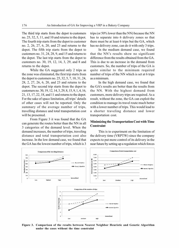
From Figure 3 it was found that the GAcan generate the routes better than the NN in all3 categories of the demand level. When thedemand increases, the number of trips, travelingdistance and total transportation cost alsoincrease. In the low demand case, we found thatthe GA has the lowest number of trips, which is 3

trips (or 50% lower than the NN) because the NNhas to separate into 6 delivery zones so thatthere must be at least 6 trips but the GA, whichhas no delivery zone, can do it with only 3 trips.

In the medium demand case, we foundthat the NN’s results show no significantdifference from the results obtained from the GA.This is due to an increase in the demand fromcustomers. So, the number of trips of the GA isquite similar to the minimum requirednumber of trips of the NN which is set at 6 tripsas a minimum.

In the high demand case, we found thatthe GA’s results are better than the results fromthe NN. With the highest demand fromcustomers, more delivery trips are required. As aresult, without the zone, the GA can exploit thecondition to manage its travel route much betterwith a lower number of trips. This would lead toa shorter traveling distance and lowertransportation cost.

Minimizing the Transportation Cost with TimeConstraint

This is to experiment on the limitation ofthe delivery time (VRPTW) since the companyexpects to put more control of its delivery in thenear future by setting up a regulation which forces

Figure 3. Comparison of the results between Nearest Neighbor Heuristic and Genetic Algorithmunder the cases without the time constraint


reduction is 465 Baht (or 7.00%). For the highdemand case, it was found that the GA canreduce the traveling distance by 35 km (or 4.21%)with a 1 trip’ reduction (or 7.69%) and the totaltransportation cost reduction is 475 Baht(or 5.90%).

According to Figure 4, for all demand cases,the NN’s results show no significantdifference from the results obtained from the GA.This is due to the fact that all vehicles need toreturn to the depot within 3 h. As a result,the vehicle cannot load the products to fullcapacity and this forces both systems (especiallythe GA) to have more trips and longer travelingdistances than usual. As a result, no significantimprovement with the GA can be presented inthis case.

Time Constraint of 4 Hours

Table 8 also summarizes the comparisonof test results between the NN and GA.Referring to the average value for the lowdemand case, it was found that the GA canreduce the traveling distance by 18 km (or 3.22%)with 2 trips’ reduction (or 33.33%) and thetotal transportation cost reduction is 690 Baht(or 15.02%). For the medium case, the GA hasthe average values higher than the ones from

each vehicle to work faster and come back to thedepot sooner. This is done by setting up a timewindow/constraint. The time window/constraintis related to the total time to deliver the productincluding the loading and unloading time,delivery time and return time. There are 3 levelsof time constraint, which are set within 3, 4, and5 h. This is corresponding to the maximumperiod of 5 h between the mid-night and 5 amwhen the delivery activities must take place.These instances can also be classified, based onthe levels of customer demand into 3 categories-low, medium and high.


Table 7 summarizes the comparison of testresults between the NN and GA for both the bestand average values. For the average value in thelow demand case, the results of the GA haveaverage values slightly higher than the ones fromthe Nearest Neighbor Heuristic that is the longertraveling distance by 27 km (or 4.83%) withan equal number of trips and a higher totaltransportation cost of 135 Baht (or 2.93%). Forthe medium demand case, it was found thatthe GA can reduce the traveling distance by33 km (or 4.53%) with a 1 trip’ reduction (or10.00%) and the total transportation cost

Figure 4. Comparison of the results between Genetic Algorithm and Nearest Neighbor under thecases with the time constraint of 3 h


the NN, which has the longer traveling distanceby 22 km (or 3.82%) with equal number oftrips and a higher total transportation cost of110 Baht (or 2.21%). For the high demandcase, it was found that the GA can reduce thetraveling distance by 62 km (or 8.27%) with2 trips’ reduction (or 18.18%) and the totaltransportation cost reduction is 910 Baht (or12.91%).

According to Figure 5, for the low demandcase, the NN’s results also suggest not muchdifference from the results obtained from theGA especially with the traveling distance due tothere still being the time constraint. However,when comparing between the 3 h and 4 h timeconstraint, it was found that the GA under the4 h time constraint has a lower number of tripsand traveling distances than the NN’s resultsbecause a vehicle can serve more products tocustomers on each trip. As a result, the totaltransportation cost obtained from the GA hasbeen shown to be lower.

In the medium case, the NN’s resultssuggest no significant difference from the resultsobtained from the GA. This is due to an increasein the demand from customers. So, the number

of trips for the GA is quite similar to the minimumrequired number of trips of the NN, which is setat 6 trips as a minimum.

In the high demand case, the GA’s resultsare much better than the NN’s results. With thehighest demand from customers, more deliverytrips are required. As a result, without the zone,the GA can exploit this condition to manage thetraveling route much better with a lower numberof trips. This would lead to a shorter travelingdistance and a lower transportation cost.


As seen in Table 9, for the average valuein the low demand case, it was found that theGA can reduce the traveling distance by64 km (or 11.45%) with 2 trips’ reduction (or33.33%), and the total transportation costreduction is 920 Baht (or 20.02%). For themedium demand case, it was found that theGA can reduce the traveling distance by 24 km(or 4.17%) with a 1 trip’ reduction or (14.28%)and the total transportation cost reductionis 420 Baht (or 8.44%). For the high demandcase, it was found that the GA can reduce thetraveling distance by 62 km (or 8.37%) with

Table 7. Comparison of test results between the Nearest Neighbor Heuristic and the GeneticAlgorithm under 3 h time constraint

DemandLevel

Performancemanner

Best value1

NN GA

Average value2

NN GA

Percentage3


values

Percentage3


values

6559

4595

9710

6250

12776

7480

5554

4270

7623

5215

10747

6735

6559

4595

10729

6645

13831

8005

6586

4730

9696

6180

12796

7580

16.67% 0.89% 7.07%

22.22%12.25%16.56%

16.67% 3.73% 9.96%

Low

Medium

High

Number of trips (trips)Traveling distance (km)Total transportation costs (Baht)Number of trips (trips)Traveling distance (km)Total transportation costs (Baht)Number of trips (trips)Traveling distance (km)Total transportation costs (Baht)

-(4.83)%(2.93)%

10.00% 4.53% 7.00%

7.69% 4.21% 5.90%





DemandLevel

Performancemanner

Best value1

NN GA

Average value2

NN GA

Percentage3


values

Percentage3


values

6559

4595

6559

4595

10724

6620

4516

3780

5531

4155

8619

5495

6559

4595

7575

4975

11750

7050

4541

3935

7597

5085

9688

6140

33.33% 7.69%17.74%

16.67% 5.01% 9.58%

20.00%14.50%16.56%

Low

Medium

High

Number of trips (trips)Traveling distance (km)Total transportationcosts (Baht)Number of trips (trips)Traveling distance (km)Total transportationcosts (Baht)Number of trips (trips)Traveling distance (km)Total transportationcosts (Baht)

33.33% 3.22%15.02%

-(3.82)%(2.21)%

18.18% 8.27%12.91%

Remark: 1. The best value's are taken from the best result among 10 replications2. The average value's results are averaged from the results of all 10 replications


3 trips’ reduction (or 27.27%) and the totaltransportation cost reduction is 1210 Baht(or 17.27%).

From Figure 6, we found that the GA cangenerate the routes better than the NN in all 3categories of the demand level. No vehicle isrequired to go back for reloading due to thelimitation on the time. This is due to the factthat more delivery time is allowed on each trip.In general, the results obtained from this caseare quite similar to the results of the no timeconstraint case. This indicates that 5 h timeconstraint would be quite sufficient to accom-modate all required trips. In the low demandcase with 5 h time constraint, the NN generates6 trips as a minimum but the GA with no deliveryzones can exploit this case to manage the travelroute better with a lower number of trips. Thiswould lead to a shorter traveling distance anda lower transportation cost.

In the medium case, the NN’s resultssuggest little difference from the results obtainedfrom the GA, although the results under the GAslightly outperform the results under the NN.This is due to an increase in the demand fromcustomers. So, the number of trips for the GA

is quite similar to the minimum required numberof trips for the NN, which is set at 6 trips as aminimum.

With the highest demand from customers,more delivery trips are required. As a result,without the zones, the GA can exploit thecondition to manage the travel route muchbetter with a lower number of trips. This wouldlead to a shorter traveling distance and a lowertransportation cost.

Comparison of the Results Obtained fromGenetic Algorithm

As the results obtained from the GA aregenerally shown to outperform the company’sexisting results using the NN, another attempt ismade to analyze specific results obtained fromthe GA under all 3 levels of the customer demandboth with and without the time constraint. Thisis to recommend the best time window if thecompany would like to limit the delivery time ofeach vehicle. The comparisons of these resultsare shown in Table 10 and Figure 7.

In the no time constraint cases, ascompared with the results under the timeconstraints, the results show the lowest number


of trips, the traveling distances and totaltransportation cost due to no limitation on thetime. Table 11 summarizes the number of extratrips for the vehicles due to the limitation of thedelivery time for both the NN and GA. From our

finding, the 5 h time constraint result showedquite a similar result to the case of no timeconstraint by having no extra trip at all. Thissuggests that 5 h would be sufficient forproduct delivery with fully loaded vehicles.




Figure 7. Comparison the results of the total transportation cost under the Genetic Algorithm


( )

DemandLevel

Performancemanner

Best value1

NN GA

Average value2

NN GA

Percentage3


values

Percentage3


values

6559

4595

6559

4595

9655

5975

3455

3175

5516

4080

8614

5470

6559

4595

7575

4975

11741

7005

4495

3675

6551

4555

8679

5795

50%20.39%30.90%

16.67% 7.69%11.21%

11.11% 6.26% 8.45%

Low

Medium

High

Number of trips (trips)Traveling distance (km)Total transportationcosts (Baht)Number of trips (trips)Traveling distance (km)Total transportationcosts (Baht)Number of trips (trips)Traveling distance (km)Total transportationcosts (Baht)

33.33%11.45%20.02%

14.28% 4.17% 8.44%

27.27% 8.37%17.27%


3. Percentage difference is calculated from Result of NN - Result of GAResult of NN x 100%

However, with 3 h time constraint, except onlyfor the low demand case with the NN, thevehicles are forced to go back to the depot inmany instances due to the limitation on the time.This leads to a significant increase in thenumber of trips, traveling distance and totaltransportation cost. Regarding the 4 h time

constraint, only in a few instances with boththe NN and GA are vehicles forced to returnto the depot due to the limitation on time. Asa result, the suitable time for controlling thedelivery time should be set around 4 h. Eventhough the 5 h time constraint cases showa similar or a bit cheaper cost than the 4 h


Table 11. The number of extra trips forced to return to the depot due to the limitation of thedelivery time

Type of Demand Number of extra tripsalgorithm level 3 h’ time constraints 4 h’ time constraints 5 h’ time constraints

Low - - -NN Medium 3 - -

High 5 1 -Low 4 2 -

GA Medium 6 1 -High 6 - -

Table 10. Comparison of the average value of number of trips, traveling distances and totaltransportation costs in 4 c ategories under the GA

L M H L M H L M H

Remark: L = Low demand caseM = Medium demand caseH = High demand case

Total transportation costs(Baht)

No. trips(trips)

Traveling distances(km)

Detail

No time constraint 3 6 8 515 556 679 3475 4580 5795Time constraint of 3 h 6 9 12 586 696 796 4730 6180 7580Time constraint of 4 h 4 7 9 541 597 688 3905 5085 6140Time constraint of 5 h 4 6 8 495 551 679 3675 4555 5795

time constraint cases, 1 h saved from deliverymeans 1 h less for customers to receive theirproducts. This could not only increase customersatisfaction but also reduce other relevantcosts of the company such as inventoryholding, warehouse operation, and manpowercosts.

Conclusions

This work studied the classical VRP problemusing real data of a bakery company. Allinformation was gathered during the internshipperiod. The company with a single depot hasto serve various types of products to itscustomers. The company currently uses a NNalgorithm with 6 delivery zones to generate theroutes of delivery. Therefore, the goal is tocompare the results between the existingapproach based on the NN and the proposedapproach based on the GA.

From the finding, we firstly recommendedan elimination of delivery zone in our proposedalgorithm with the GA because the resultswithout the zone clearly showed a shorter

delivery time and lower transportation cost.Currently, with only 32 customers, it appearedthat there is no need to divide them into zones.However, when more customers are added in thefuture, delivery within zone may be more usefulsince each vehicle can serve its own customersmore closely and more rapidly. Anotherrequirement is the time window when thecompany would like to limit the delivery time ofeach vehicle in the future. With the timeconstraint of 3 h, all results have increased sincethe vehicles are forced to return to the depotwithin 3 h. As a result, more trips are required.With 4 h time constraint, more time is allowedfor delivery so a lower number of trips can becarried out. This leads to a lower travelingdistance and total transportation cost. Theresults of 5 h time constraint appeared to besimilar to the ones from the no time constraintcase. Since the longest time is allowed for eachtrip, the vehicles would not be forced by thelimitation on the time to go back to the depotduring the trip. As a result, the 4 h timeconstraint was recommended to the companysince one hour limited from each trip means


1 h less for customers to receive their products.This 1 h saved from each trip could save a lot ofcosts for the company, which costs are notincluded in our calculated total transportationcosts.

Under the comparison between theexisting system operation under the NN and theproposed system operating under the GA, theGA’s results generally outperform the NN’sresults. Only when the demand is medium arethe NN’s and the GA’s results quite close. Whenthe demand is low or high, the system under theGA clearly showed better results with a lowernumber of trips, traveling distances and totaltransportation cost. As a result, it may bepossible to conclude that the GA could improvethe vehicle routing of this bakery company andsave the total transportation cost up to 20% ascompared with the existing method used by thecompany. According to the finding, the companycan select an appropriate route matching withthe suitable demand level. The recommendationhas already been passed to the company and itis in their consideration to implement thisfinding.

This problem is of economic importanceto businesses because of time and costsassociated with providing a fleet of deliveryvehicles to transport products to a set ofgeographically dispersed customers. It involvesfinding the minimum cost of the combined routesfor a number of vehicles in order to facilitatedelivery from a supply location to a number ofcustomer locations. Since cost is closelyassociated with distance, a company mightattempt to find the minimum distance traveledby a number of vehicles in order to satisfy itscustomer demand. In doing so, the companyattempts to minimize costs while increasing or atleast maintaining an expected level of customerservice. As a result, the accuracy of a company’scost structure plays an important role inobtaining good results. In fact, it is quitedifficult for a company to commit to somenumbers in its cost structure since they havenever been recorded or, in many instances,managers are hesitant to estimate them.Moreover, the cost structure varies from onecompany (industry) to the other. As poor inputs

lead to poor results, without a reliable coststructure, the obtained results could be mis-leading and could lead to misinterpretation.Sensitivity analysis could also be conducted withrespect to some cost parameters to check theirinfluence on the results.

Nevertheless, this approach can also beapplied to other types of VRP application suchas delivering perishable food or fresh food inwhich a similar condition applies. Further studycan also be extended to other situations such ascomparing the results under the GA with otheralgorithms (such as Tabu Search, Particle Swarm,etc.) aiming to search for a better result. Inaddition, a greater number of customers can alsobe added to the current situation. This will makethe size of the problem larger and clearlyhighlight the differences of our proposedalgorithm to the existing one. A modificationof the transportation cost function could alsobe done to reflect greater reality. With thiscase,the transportation cost is merely a directcharge from the delivery distance. As a result,the transportation cost is directly varied withthe distance traveled. So, optimizing thetransportation cost is always in line withoptimizing the delivery distances. Addingother cost factors to the transportation cost mayresult in new interesting findings to the outcomeof the study.

AcknowledgementThis work was supported by the HigherEducation Research Promotion and NationalResearch University Project of Thailand Officeof the Higher Education Commission andNational Science and Technology DevelopmentAgency (NSTDA) through U-IRC program. Theauthors are also grateful for the valuablecomments and suggestion from the respectedreviewers. Their valuable comments andsuggestions have enhanced the strength andsignificance of our paper.

ReferencesBaker, B.M. and Ayechew, M.A. (2003). A genetic

algorithm for the vehicle routing problem.Computers & Operations Research, 30:787-800.


Bell, J.E. and McMullen, P.R. (2004). Ant colonyoptimization techniques for the vehicle routingproblem. Advanced Engineering Informatics,18:41-48.

Braysy, O. and Gendreau, M. (2005). Vehicle routingproblem with time windows. TransportationScience, 39:119-139.

Chidananda, G. and Krishna, G. (1979). The condensednearest neighbor rule using the concept ofmutual nearest neighborhood. IEEE Transactionson Information Theory, 25(4):488-490.

Dantzig, G.B. and Ramser, J.H. (1959). The truckdispatching problem. Management Science,6(1):80-91.

de Oliveira, H.C.B., Vasconcelos, G.C. and Alvarenga,G.B. (2006). A multi-start simulated annealingalgorithm for the vehicle routing problem withtime windows. Proceedings of the Ninth BrazilianSymposium on Neural Networks (SBRN’06).27 October, 23:137-142.

Gambardella, L.M., Taillard, E. and Agazzi, G. (1999).MACS VRPTW: A Multiple Ant Colony Systemfor Vehicle Routing Problems with TimeWindows, New Ideas in Optimization, McGrawHill Ltd., Maidenhead, UK.

Ghoseiri, K. and Ghannadpour, S.F. (2010). Multi-objective vehicle routing problem with timewindows using goal programming and geneticalgorithm. Applied Soft Computing, 10:1096-1107.

Holland, J.H. (1975). Adaptive in Natural and ArtificialSystems. The University of Michigan Press, AnnArbor, MI.

Jeon, G., Leep, H.R. and Shim, J.Y. (2007). A vehiclerouting problem solved by using a hybrid geneticalgorithm. Computers and Industrial Engineer-ing, 53:680-692.

Jigang, W., Predrag, N., and Leon, N.C. (2007).Improving nearest neighbor rule with a simpleadaptive distance measure. Pattern RecognitionLetters, 28:207-213.

Prins, C. (2004). A simple and effective evolutionaryalgorithm for the vehicle routing problem.Computers and Operations Research, 31:1985-2002.

Poon, P.W. and Carter, J.N. (1995). Genetic algorithmcrossover operators for ordering applications.Computers Operations Research, 22(1):135-147.

Su, C.T. (1998). Locations and vehicle routing designsof physical distribution systems. ProductionPlanning & Control, 9(7):650-659.

Taillard, E. (1993). Parallel iterative search methodsfor vehicle routing problems. Networks, 23:661-673.

Toth, P. and Vigo, D. (2002). The Vehicle Routing Problem.SIAM Monographs Discrete Mathematics andApplications. Society for Industrial and AppliedMathematics, Philadelphia, USA.

Zhou, C.Y. and Chen, Y.Q. (2006). Improving nearestneighbor classification with cam weighteddistance. Pattern Recognition, 39:635-645.

Documents

AN INTRODUCTION OF GENETIC ALGORITHM FOR An Introduction of GA for Improving a VRP in a Bakery Company performance of a bakery company with a single depot by introducing the Genetic