An interlayer model for the complex dielectric constant of composites

Colloid & Polymer Science Colloid Polym Sci 268:315-325 (1990)

An interlayer model for the complex dielectric constant of composites

P. A. M. Steeman and E H. J. Maurer

DSM Research BV, Geleen, The Netherlands

Abstract: The complex dielectric constant of a composite with an interlayer was studied as a function of the volume fractions and the properties of the filler, the interlayer, and the matrix. The theoretical approach is analogous to the calculation of the shear modulus, the bulk modulus, and the termal expansivity of particulate filled polymers using the interlayer model (IM). An analytical expression describing the influence of an interlayer on the generalized dielectric constant of the composite as a function of the volume fraction and interlayer properties is derived. In the case of a composite with non-conductive constituents, the equations for static and oscillatory electric fields are similar. When conductive constituents are present, the complex dielectric constants have to be replaced by the generalized complex dielectric constants. For a composite of non-conductive materials, without interlayer, the obtained relation reduces to the classical Rayleigh equation. In the case of a composite with conductive constituents, also without interlayer, the complete solution of Wagner's theory is found. Special attention has been paid to the case of a water interlayer in a glass-bead filled non-conductive matrix material.

Key words: _Interlayer model; dielectric c_onstant; composite; filled Eolymer; i_nterfacial water

Introduction

The description of the physical properties of composites (or, more in general, heterogeneous materials) based on the volume fractions and properties of the constituents and the morphology has been a subject of interest for several decades. Recently, attention was focused on the description of the influence of the interactions between the constituents and the influence of a possible resulting interlayer.

Analogous to a method used by Fr6hlich and Sack [1] and by van der Poel [2] for the description of the viscosity and shear modulus of particulate filled systems without interlayer, Maurer derived an interlayer model (IM) for the description of the shear modulus G [3], the bulk modulus K [4], and the thermal expansivity c~ [4, 5]. The relations between the molecu- lar interactions and the interlayer properties are in- vestigated by comparing the thermal expansivity o~ [4, 5] and the bulk modulus K [6] as obtained from

a statistical mechanical lattice model (MM), with those obtained by the micro-mechanical approach.

The analogy between the mechanical and the electrical field equations suggests that it is possible to describe the dielectric properties of a particulate filled composite with interlayer, also with the interlayer model.

An investigation of the effects of an interlayer, for instance water adsorbed at the filler-matrix interface, is of practical interest. Adsorbed water at the filler/fiber-matrix interface can have an adverse effect on the properties of composite systems. Since the presence of water can be detected very sensitively using dielectric measurement techniques, insight into the interpretation of the measured loss effects could lead to a better understanding of practical composite systems.

The presence of water in composite systems and its detection by dielectric methods is known from

K 677

316 Colloid and Polymer Science, Vol. 268 �9 No. 4 (1990)

literature [7-10]. However, a clear analysis of the data is often not possible because of the complexity of the systems under investigation and the lack of insight into the physical phenomena, even under extremely simplified conditions such as for particulate filled systems.

The aim of the work to be presented here is to show the basic parameters involved and some important relations between the properties of the constituents and the dielectric properties of the composite on the basis of the interlayer model.

Some theoretical work on the dielectric properties of three phase systems is known from literature [11- 13]. Pauly and Schwan [11] and Hanai [12] give an analytical expression for the dielectric behavior of suspensions of spherical particles with a surface layer. They show that for frequency independent material properties of the constituents in general two retardation processes are found in the frequency domain. Tinga [13] derived an analytical expression for the dielectric properties of three-phase systems with eUipsoidal inclusions.

In this paper we first derive the interlayer model for the static dielectric constant of a composite of non-conductive materials. Using the correspondence principle, this formula can be extended to oscillating fields. The resulting model will be extended to conductive materials by introducing the generalized complex dielectric constant.

The interlayer model is finally simplified for a composite in which only the interlayer is conductive. In this case a single retardation process of the Debye type is observed, as shown. This important special case is very interesting as it can be used to describe the dielectric effects of water adsorbed at the filler- matrix interface in composite systems.

In the discussion we present some experimental results on the water absorption of particulate (glass- bead) filled polyethylene and show how the developed interlayer model is able to describe and give insight into the detected dielectric loss processes.

Fig. 1. Model of a composite with interlayer.

matrix material while further away the overall composite properties describe the system. The RVE, as defined, is depicted in Fig. 1. The radii of the shells are chosen in a way corresponding to the volume fractions, i.e.,

~f = a3, ~ = b3 - a3, ~m = 1 - b 3 . (1)

We assume that the response of this RVE to an externally applied electric field equals the response of a volume element of pure composite material. The electrical potential V in a homogeneous, isotropic material in which no free space charge is present can be obtained from the Laplace equation

A~,= 0. (2)

The general cylindrically symmetric solution of this differential equation in spherical coordinates, using Legendre polynomials, is given by

0 o

V = ~ (Anrn + B n / r n + 1). Pn (cos 8). n = 0

(3)

The static dielectric constant

Consider a particulate filled composite consisting of spherical filler particles, surrounded by an interlayer, and dispersed into a matrix. We take a repre- sentative volume element (RVE) which contains one filler particle, surrounded by an interlayer. In the immediate vicinity of the interlayer there is pure

Due to the application of an external homogeneous electrical field E o, in the 8 = 0 direction, the potential in the composite equals

V = E o �9 r . cos(~) . (4)

The electrical potential in the different areas of the RVE can be described by

Steeman and Maurer, An interlayer model for the complex dielectric constant of composites 317

~/f = ~(An[f]r n + Bn[f]/rn+') �9 Pn(cosS) , n=O

= ~ ( A n [ l ] r n + Bn[l l /rn+l) . Pn(COSO) , n=O

Y/m = ~ ( A n [m]rn + Bn [m] / r r + 1). Pn(COS0) , n=0

(5)

(6)

(7)

r = ~--,(AnIC] rn + Bn[ c]/rn + 1). Pn(C.os~ ) . (8) n=O

At the boundar ies be tween the different materials the electric potential and the normal component of the dielectric displacement must be continuous. The normal component of the dielectric displacement D n is given by

D n = - e . ~ (9) Or "

Moreover, the potential at r = 0 must be finite, while the potential for r > 1 must be equal to the potential in a homogeneous material wi th the overall material parameters of the composite, which we want to determine. Because of these bounda ry and con- t inui ty conditions we find the following relations for the A n [i] and B n [i] coeff• with n = 0,1... and i = c, f , l, m, i f e i with i = f, l, m stands for the relative dielectric constant of the filler, the layer, and the matrix, respectivel~

F o r n = l a t r = a w e f i n d Ba[f] = 0 a n d

Al[f] . a = AI[I] . a + B,[ l ] /a 2 (I)

el. AI[ f] = e t �9 (AI[/] - 2 . Bl[ l l / a 3) .

F o r n = l a t r = b w e f i n d

(II)

AI[ l ] �9 b + BI[ l ] /b 2 = AI[ m ] �9 b + B l [ m ] / b 2 . (III)

e l �9 (AI[/] - 2 . Bl[ l ] /b 3) = e m �9 (Al[m] - 2 . B l [ m ] / b 3 ) .

(iv)

F o r n = l a t r = l w e f i n d B l [ c ] = 0 a n d

Aa[m] + Bl[m] = Al[c] (V)

e m �9 (A, [m]- 2 . B , [ml )=e e �9 A 1 [c] . (VI)

The electric field at r > 1 must be equal to the external homogeneous field. For n r 1, we therefore find that, using the continui ty conditions, A n [i] = 0 and B n [i] = 0 with i = c, f, 1, m. The six remaining equations ( I ) - ( VI ) contain the six u n k n o w n parameters A 1 [ f ], A 1 [ 1 ], B 1 [ 1 ], A 1 [m], B 1 [m], A 1 [c], and the dielectric constant e c of the composite for which we want to solve the equations. In order to get a non-trivial solution of these equations the de- terminant of the coefficients of the six u n k n o w n parameters should vanish:

a - a - a -2 0 0 0

8 f - e l 28t a-3 0 0 0

0 b b -2 - b - b -2 0

0 e l -281 b-3 - e m 28m b-3 0

0 0 0 1 1 - 1

0 0 0 em -2em - G

=0

After matrix manipulat ions the following expression for the static dielectric constant of the composi te e c can be der ived

erO~+ e ~ r + em r

r = 4)i + 4~ R + r S ' (10)

wi th

2et+ ef R = (11)

3e l '

S = (2e I + el) (2e m + e l ) - 2 d . (e I - em) (e l

9 e m e I

(12)

and

d- 0f (13) r162

Consider a composi te wi thout interlayer, i. e., a composi te for which in Eq. (10) the layer vo lume

318 Colloid and Polymer Science, Vol. 268. No. 4 (1990)

fraction r is set to zero. Relation (10) then reduces to

(2 e m + @ + 2 (el- em)(~ f

ec=am (2 em + @_ (of_ ~m)@ f (14)

This relation is equal to the Rayleigh solution [14] for the dielectric constant of a system with dispersed spheres. From this equation we derive the reduced value of the dielectric constant of the composite as

e c - e m _ 3 ( e f - e m )

emr ( 2 e , , , + e f ) - ( e f - e , , 3 el" (15)

The intrinsic value of the dielectric constant of the composite is equal to the limit of the reduced value for zero filler volume fraction

(e c - em~ 9e m lira - - --3 #/~0 f Em~f ) 2Em+Ef

(16)

In Fig. 2 we have depicted the reduced value of the dielectric constant of a composite without interlayer as a funtion of the filler volume fraction, as

5.0 �84

4.0

3.0

2,0

1.0-

0.0

-1 .0 -

-2.0-

0.0

(~c-- EM

EM ~)f 6F / ~M

~ 100000 100

.5

,1 0.00001

- - i ~ - - Volume fraction ~)F

o11 o12 o13

Fig. 2. The reduced va lue of the dielectric constant of a composi te wi thout interlayer as a funct ion of the filler v o l u m e fraction for several ratios of the filler and the matr ix dielectric constants.

Lira E c - E M 3.0 ~F__~. 0 EM~F

2.0 I

1.0-

0.0

-1.0

log (6f / EM', - 2 . 0 l i i I t

- 4 - 2 0 2 4

Fig. 3. The intrinsic va lue of the dielectric constant of a composi te wi thout interlayer as a funct ion of the ratio of the filler and the matr ix dielectric constants.

calculated for several ratios of the filler and the matrix dielectric constant. For small filler volume fractions, the reduced value is only slightly dependent on the filler volume fraction, while the ratio of the dielectric constants has a very large influence. In Fig. 3 we have depicted the intrinsic value of the composite dielectric constant as a function of the logarithm of the ratio of the dielec~ic constants of the filler and the matrix material. As can be seen, we find two limiting values, namely -1.5 and +3, with a relatively sharp transition in the range 0.1 < ef / e,, < 10.

In Table I we summarize the intrinsic values that were previously obtained for the shear and bulk modulus [3, 4], the viscosity [3], and the thermal expansivity [4, 5] from similar derivations.

Table 1: Intrinsic va lues

Property Symbol Intr. va lue Condi t ions

Expansivi ty ~z -1 ~ <<r K i >> G i Bulk m o d u l u s K 1 Kf >> Km; K m >> G m Shear m o d u l u s G 2.5 Gf >> Gin; K m >> G m Viscosity r/ 2.5 Gf >> Gin; K m >> G m Dielectric cons tant e 3 ef >> em

The dynamic dielectric constant

Consider a harmonically oscillating electric field with amplitude E o and angular frequency 09, as re-


presented in Eq. [17], which is applied to a composite with non-conductive constituents

E*(t) = E o �9 d r~ . (17)

We define the complex dielectric constant of a material e*(c0) as the ratio of the complex scalar dielectric dis~placement D*(t) and the complex scalar electric field E (t) in the material when a harmonically oscillating field is applied [15]:

D*(t) = d ( c o ) . E*(t) . (18)

The complex dielectric constant e* (co) of a material is usually specified by its real and imaginary parts according to relation (19):

d(CO) = e'(ca) - i. d'(cO), (19)

in which g(c0) is the frequency dependent dielectric constant of the material and g'(co) the frequency dependent loss index of the material.

Using the complex dielectric constant defined as such, the correspondence principle states that Eq. (10) for the dielectric constant of the composite also applies to oscillatory fields, when we replace the static dielectric constant ei by the complex dielectric constant e i , i = c, f , l ,m.

The dielectric constant of a c o m p o s i t e of conduc- t ive materials

If the composite contains conductive materials we have to take into account that some accumulation of charge at the boundaries may occur. Therefore, we have to examine the field equations and the boundary conditions that were used before. The field equation (2) still holds, but the boundary condition stating that the normal component of the dielectric displacement is continuous no longer holds. Following B6tt- cher [15] we define for harmonic fields the generalized complex dielectric displacement D* (t) as

t

D*(t) = D*(t ) + ; j*(t ' ) dt ' , (20)

where j*(t) is the complex free current density in the material. It can be shown that the generalized com-

plex dielectric displacement D*(t) and the complex harmonic electric field E (t) are related via the generalized complex dielectric constant _e*(r [15]:

D*(t) = __e*(co) �9 E*(t), (21)

with

d(o~) e_*(co) = d ( r o ) + i m "

where e*(co) is the complex dielectric constant of the material and o-*(c0) is the complex conductivity of the material. The generalized complex dielectric displacement can be shown to be divergence-free [15]. Therefore the new boundary condition to be used states that the normal component of D_* (t), defined a s

D ,(t) = - _e*(co) �9 3V(t) (22) Or '

should be continuous at the boundaries. The second boundary condition, continuity of the electric potential at the boundary, still holds.

Using the general solution (3) of the potential equation and the new boundary conditions we finally obtain the generalized dielectric constant of the composite as a function of the properties and the volume fractions of the constituents. The obtained relation is identical with the static solution after replacement of the static dielectric constants e i by the generalized complex dielectric constants _e i fro), with i = c, f, l, m :

=

09

_~(o~) �9 0~+_eT(o~) �9 0 t " R*(o~) + ~ ( o J ) �9 ~m" S*(co)

~i+ r R*(oJ) + ~m" S*(o~) (23)

with

R*(co) = 2e~(c0) + _~(co)

3e~(co) (24)


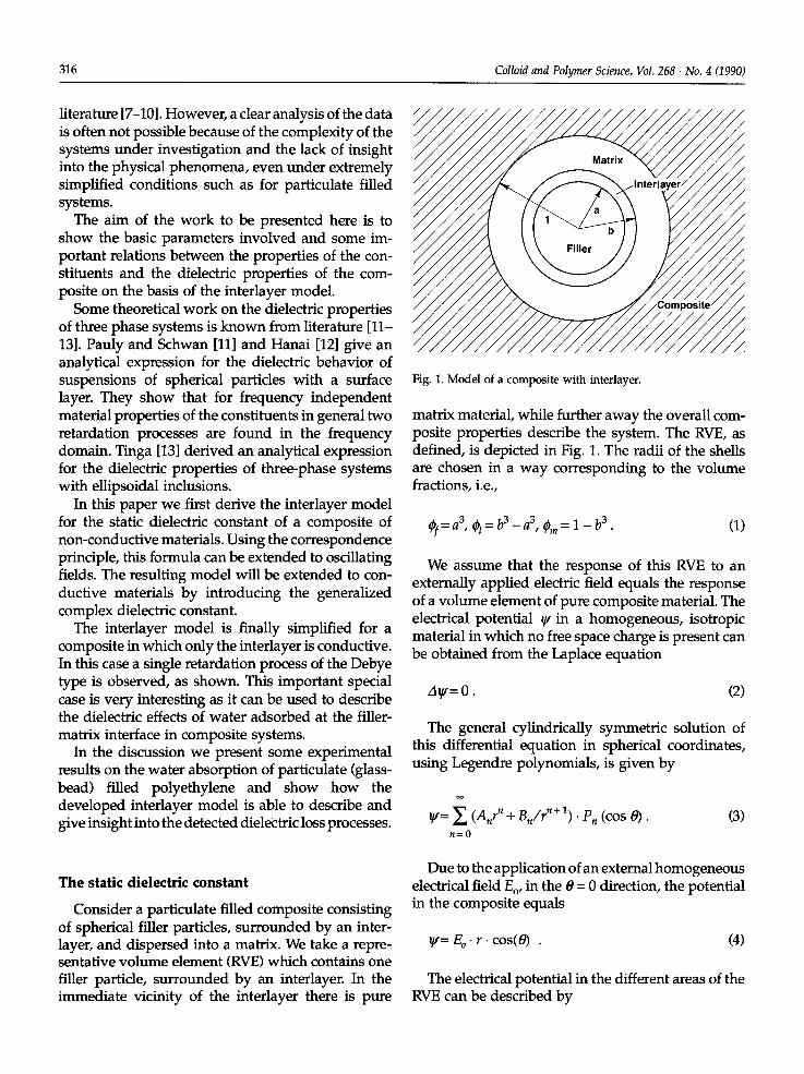
S*(co) (2e~(co) + -~(co)) (2e-~n(t~ + ~(co)) - 2d(-~*(c~ - e-~n(t~ (-eJ* (co) - -~ (co)) = and

9e~(co) e_~(co) (25)

(26)

Here_ei* (co) is the generalized complex dielectric constant and r the volume fraction of the filler, layer or matrix, for i = f, I, m, repectively.

The interlayer model as derived can~be used to calculate the dielectric behavior of any three-phase composite with spherical inclusions. In the case of a composite in which the constituents have frequency- dependent dielectric properties the dielectric constant and loss index of the constituents should be inserted directly in the basic formula, for each frequency separately. The composite dielectric constant and loss index calculated with formula (23) are equal to the results obtained from the relations as derived by Pauly and Schwan [11l, Hanai [12], and Tinga [13]. On the contrary to the other relations, the interlayer formula (23) as derived is very easy to handle and can be easily simplified in special cases such as for two-phase composites, or for the case of a three-phase composite in which only the interlayer is conductive, as will be shown. Equation (23) is similar to the expressions obtained for the bulk modulus [4] and the thermal expansivity [5] of composites described by the interlayer model which might, in some cases, lead to additional insight.

Consider a composite without interlayer, i. e., a composite for which in Eq. (23) the layer volume fraction ~I is set to zero. Eq. (23) then reduces to

�9 , (2e_~n(co) + _~(co)) + 2 �9 (_~(co) - e_~(co)) ' @f ~ ( c o ) = ~ ( c o ) , , , , .

(2em(co) + ef(co)) - (ef(co) - em(co)). ~df(27)

This relation is equal to the complete solution of Wagner's theory [14] for the generalized complex dielectric constant of a composite with dispersed conducting spheres.

The dielectric behavior of composite with a conductive interlayer

Consider a composite in which only the interlayer is conductive and assume that this, conductivity is frequency independent. Assume furthermore thai the dielectric constants of the filler, layer, and matrix materials are also frequency independent. These ap- proximations may for instance be used to describe the audio-frequency dielectric behavior of glass bead filled polyethylene (HDPE) samples in which water is adsorbed at the glass (filler) surface.

If the volume fraction of the layer r is much smaller than the filler volume fraction qf, and the dielectric constant of the layer is much smaller than the conductivity of the layer divided by the angular frequenc35 it can be shown that formula (23) reduces to a Debye-type dispersion:

e0-e~ F(co) = = + 7+9 , ( 2 8 )

in which

r )" (29)

(ef+ 2e m) + 2. (ef- em). qbf e . = em ( e I + 2em) - ( e i - era)" ~f '

(30)

and

v = ( - ~ l . r 2em)-(ef-em)(~f] (31) ~1- ~ j t2crl~)

where eo is the low frequency limit of the composite dielectric constant, e~ is the high frequency limit of the composite dielectric constant, and ~ is the retardation time of the loss process, respectively. The vacuum permittivity ewe in this relation equals 8.85 pF/m.

The low frequency permittivity e o of the composite is completely determined by the volume fraction of the filler qfand the dielectric constant em of the matrix material. The conductive layer effectively shields the electric field from the filler particles. We have, in fact, a composite of a non-conductive matrix with highly conductive spheres dispersed in it.


Equation (30) for the high frequency permittivity e~ is equal to the Rayleigh equation (14) for the dielectric constant of a composite of non-conductive spheres dispersed in a non-conductive matrix.

From relation (31), giving the retardation time of the loss process ~:, it appears that the frequency of maximum dielectric loss, caused by the effect of the conductive interlayer, is proportional to both the volume fraction ~)t and the conductivity ~ of the interlayer.

Discussion

We first discuss the influence of an interlayer on the static dielectric constant of a composite, according to Eq. (10). The static dielectric constant of a composite with e f / e m = 5 is depicted in Fig. 4, as a function of the logarithm of the ratio fo the dielectric constants of the layer and the matrix, for several values of the layer volume fraction r We can distin- guish three characteristic el/em ranges in this figure. For e l << e m the static dielectric constant of the composite with interlayer has a limiting value which is smaller than the static dielectric constant of the composite without interlayer. The electric field lines tend to lie parallel to the filler surface. The filler/layer properties are completely governed by the layer dielectric constant and the sum of the filler and layer

E C [E M

4 .0 - I

3 .0

1.0-

0.0 J - 2 - 1 0

2.0 �84

E F [E M = 5

q)F = .3 .2

.05

.001

~ l o g (E~/~:M) i

Fig. 4. The relative static dielectric constant of a composite with interlayer as a function of the ratio of the layer and the matrix dielectric constants for layer volume fractions of 0.001, 0.05, and 0.2.

volume fractions. For e l - e f the composite static dielectric constant tends to the dielectric constant of a composite without interlayer in which the fillel volume fraction equals the sum of the filler and layer volume fractions in the composite as considered here For higher layer dielectric constant the compositr dielectric constant increases to its final limiting value. This limit for e 1 > > ~m equals the static dielectric constant of a composite in which conducting particles are dispersed. The volume fraction of the particles equals the sum of the filler and the layer volume fractions. Because of the very high dielectric constant of the layer, the electric field lines are perpendicular to the layer surface. The field strength in the layer goes to zero with increasing layer dielectric constant. The layer, therefore, effectively screens off the filler particles from the electric field.

Next we simulate the influence of a conductive (water) interlayer on the complex dielectric constant in a 20 volume % glass-bead filled polyethylene composite according to Eq. (23). The dielectric constant of HDPE is about 2.4 and frequency independent. The dielectric constant of the filler is about 5.5. The filler, like the matrix, has no electrical conductivi~ the conductivity of the water interlayer is chosen to be 0.01 (a'-2m) -1, frequency independent. We observe in Figs. 5 and 6 for 10 -8 < r < 10 -4 a loss peak in the frequency domain from 0.1 Hz to 50 kHz. The volume fraction of the interlayer and the peak frequency are proportional to each other, as derived earlier. The shape of the loss curve is the same for all (small)

4.5

4.0

3.5

3.0

2.5

Dielectric Constant E~

~|=10 -e

\ - - ;~ - - - Iog (Frequency / [Hz])j

-t ~ ~ ~ ~ ,~ s

Fig. 5. The dielectric constant of a composite with a conductive interlayer as a function of frequency and layer volume fraction. The volume fraction of the layer as indicated.

322 Colloid and Polymer Science, Vol. 268. No. 4 (1990)

0.80- Loss Index E~

I ~ [ =10 -6 10-7 10-6 10-3 10-4 10-3

0 . 6 0 -

0.40

0.20

0.00 -- log (Frequency I [Hz])

-1 ~ i ~ ~

Fig. 6. The loss index of a composite wi th a conduct ive interlayer as a funct ion of frequency and layer vo lume fraction. The vo lume fraction of the layer as indicated.

layer volume fractions. The curve is shifted along the frequency axis to higher frequencies with increasing layer volume fraction.

When we simulate the influence of the layer conductivity on the dielectric loss we obtain similar figures, since the layer conductivity and volume fraction are interchangeable, as can be seen from formula (31).

The influence of the dielectric constant of the filler particles is simulated in Figs. 7 and 8. The low frequency dielectric constant of the composite is shown to be independent of the filler dielectric con- 4.5

4,0-

3.5-

3.0-

2.5 �84

2.0 �84

Dielectric Constant ~'~:

-1 0 1

Ef

32

16

8

4

2

I - - ~ ' - log (Frequency I [Hz]) [

Fig. 7. The dielectric constant of a composi te wi th a conduct ive interlayer as a funct ion of frequency and filler dielectric constant. Dielectric constant of the filler as indicated.

1"2 t ioss Index E~

1.0 E f 2

0.8q

0 . 6 -

0.4-

0.2-

0.0 ]

-1

- - i ~ ' - I o g (Frequency / [Hz])

1 2 3 4 5

Fig. 8. The loss index of a composite wi th a conduct ive interlayer as a funct ion of frequency and filler dielectric constant. The dielectric constant of the filler as indicated.

stant. At low frequencies the electric field is excluded from the interlayer because of the electrical conductivity of the interlayer. The dielectric constant of the particles with the conductive interlayer is infinitely high. The electric field is effectively screened from the filler particles. The high frequency dielectric constant of the composite is, on the contrary, strongly dependent on the filler dielectric constant. With increasing dielectric constant of the filler, we see an increasing high-frequency limit and a decreasing peak height of the loss process. The peak frequency slightly decreases with increasing filler dielectric constant.

The influence of the volume fraction of the filler particles is shown in Figs. 9 and 10. Both the low and the high-frequency limits of the composite dielectric constant are dependent on the filler volume fraction. The influence on the low-frequency limit is much more pronounced because of the infinitely high dielectricconstant of the particles with the conductive layer at very low frequencies. The dielectric constant of the particles with layer at high frequencies is equal to the filler dielectric constant. With increasing filler volume fraction, we see that both the low- and the high-frequency limits of the composite dielectric constant increase. The peak height of the loss process also increases, while the peak frequency slightly decreases.

A practical example of the above described phenomena can be observed in a set of dried, 20 volume


6.0-

5.0

4.0

3.0

2.0

Dielectric Constant E~;

0.3

0.25

0.2

0.15

0.1

~f

-~ l~= ' l og (Frequency / [Hz I

10 measurement frequencies per decade, using a Solartron Frequency Response Analyser type 1250 and a TNO build electrometer. In this frequency domain HDPE has a frequency-independent dielectric constant of 2.4. The glass particles have an also frequency-independent dielectric constant of 5.5.

The measured data of Figs. 11 and 12 show at least qualitative agreement with the phenomena predicted by the theory. A loss peak is observed in the experimental window at room temperature. The position of the maximum of the loss process is shifted to higher frequencies with increasing amount of water absorbed.

The observed loss peaks are much broader than the predicted Debye type. In polymeric materials

6 I ~ ~ ~ broader peaks are nearly always observed. The peak broadening is a result of a distribution in retardation

Fig. 9. The dielectric constant of a composite with a conductive times. This distribution might in our case be caused interlayer as a function of frequency and filler volume fraction, by the distribution in particle size of the dispersed The volume fraction of the filler as indicated, glass spheres resulting in a range of thicknesses of

1.2 the adsorbed water layers. As a possible modificatio n of the theory in order to describe the observed

1.0 broader loss peaks we could use the Cole-Cole relation (32) instead of the Debye relation (28). This re-

0.8 lation incorporates a symmetric broadening of the loss curves which is described by the broadening parameter a (0<a< 1 and r = 1 for a Debye loss

0.6 process ). The Cole-Cole relation is given by [16]

0.4

0.2 5.5]l~ielectric Constant C

0"11 0 1 2 3 4 5 4.5

4.0 Fig. 10. The loss index of a composite with a conductive interlayer as a function of frequency and filler volume fraction. The volume

a o o te 1 % glass-bead filled, HDPE samples exposed, at room 3.0 temperature, to different relative humidities. The mass gain and the dielectric properties were moni- 2.5 tored during the water absorption process. The z])

frequency dependent dielectric constant e' and the -1 . . . . . 0 1 2 3 dielectric loss index E" of these samples, after an equilibrium mass gain of 0.13, 0.19, 0.22, and 0.27

Fig. 11 Experimental data of the dielectric constant of a 20 volume mass %, respectively, are depicted in Figs. 11 and 12. % glass-bead filled polyethylene sample at water contents of 0.13 Data were collected between 0.1 Hz and 50 kHz with %, 0.19 %, 0.22 %, and 0;27 % at 23 ~ C.


e*(rg) = e~ ~ e~ - e . (32) (1 +jar0 r

Table 2 summarizes the Cole-Cole parameters that were obtained from a least squares fit of the experimental dielectric data of the equilibrated glass-HDPE samples. Both the dielectric constant and the loss index were used in the parameter estimation pro- gramm, based on a Newton iteration technique, in order to obtain the best possible fit. From Figs. 11 and 12 it appears that besides the predicted loss process, all samples also show an additional very low frequency (less than 5 Hz) dispersion. This dispersion may result from polarization effects at the surface or some other yet unknown effects. As a result, the low frequency permittivity increases with decreasing frequeny. The effect is most pronounced in the sample with 0.27% water uptake where also the loss index shows the onset of a very low frequency dispersion. The very low frequency dielectric data were therefore omitted from the Cole-Cole parameter fit.

0.50-

Loss Index E~

0.40-

0.30-

0.20-

0.10-

0.00

Table 2. Cole-Cole parameters

m a s s e o e~ "t [sec] a gain %

0.13 % 4.70 __+ 0.05 2.95 + 0.05 (1.75 + 0 . 0 5 ) ' 1 0 -1 0.67 + 0.01 0.19 % 4.49 + 0.05 2.95 + 0.05 (4.40 + 0.10) . 10 -3 0.66 + 0.02 0.22 % 4.53 + 0.05 2.98 + 0.05 (3.06 + 0.05) . 10 -4 0.61 + 0.02 0.27 % 4.91 + 0.05 3.18 + 0.05 (1.03 + 0.05) . 10 -5 0.60 + 0.01

O.6O -

log (Frequency / [Hz]) -1 6 i ~ ~ ~ s

Fig. 12. Experimental data of the loss index of a 20 vo lume % glass-bead filled polyethylene sample at water contents of 0.13 %, 0.19 %, 0.22 %, and 0.27 % at 23" C.

From the interlayer model we obtain for the low frequency limit~of the dielectric constant e o = 4.20, for the high frequency limit e, = 2.86, and for the broadening parameter a = 1. The experimentally obtained high frequency limits of the composite dielectric constant agreee fairly well with the theoretically calculated value, only the 0.27 % samples shows some deviation. The experimental low frequency limits of the composite dielectric constant are about 0.2 to 0.7 higher than the theoretically calculated value.

From relation (31) one would expect the retardation time of the loss process to be inversely proportional to the amount of absorbed water ff the layer conductivity was assumed to have the same constant value for all samples. The experimentally obtained retardation times depend very strongly, more than inversely proportional, on the amount of absorbed water. This can only be explained if the water layer conductivity depends on the layer thickness. It is therefore important to gain some knowledge on the conductivity of thin water layers on glass surfaces as a function of the layer thickness.

Fripiat [17] studied the conductivity of thin water films on powdered glass. The conductivity of the water layer is, at coverages greater than one molecu- lar layer, an exponential function of the layer thickness. The conductivity is mainly cationic and arises from the transfer of metal cations through the water layer driven by the electric field.

In our case the water layer thickness is linearly proportional to the amount of water absorbed by the

Log (Fma x ! [Hz]) .O/

3-

2- / AM% 0 • 0.13%

0 0.19%

1 z~ O.22% 0 0.27%

0

- - ~ - - rel, mass gain [%]

o13 o.o o'1 0'.2 Fig. 13. The logar i thm of the f requency of max imal dielectric loss as a funct ion of the relative mass ga in (in percent) of the samples .


composite. In Fig. 13 we have depicted the logarithm of the frequency of maximal dielectric loss as function of the relative mass gain due to water absorption. A linear relation between the logarithm of the loss peak frequency and the water uptake is obtained. The shifting of the frequency of maximal dielectric loss is thus mainly governed by the increase of the layer conductivity with increasing layer thickness. The layer volume fraction plays a minor role in this shifting process.

More detailed experiments monitoring the dielectric properties during water absorption of HDPE- glass composites and a quantitative evaluation of the dielectric data will be presented elsewhere [18,19].

Conclusions

Analogous to the description of the shear modulus, the bulk modulus and the thermal expansivity of particulate filled polymers with the interlayer mode l we derived the complex dielectric constant of a composite with an interlayer, as a function of the volume fractions and the properties of the filler, the interlayer, and the matrix.

The relation for the complex dielectric constant, as derived, is similar to the relation that was obtained for the bulk modulus of the composite.

In the case of a composite of non-conductive materials, we find the same equation for both static and oscillatory electric fields. However, when conductive constituents are present, the complex dielectric constant has to be replaced by the generalized complex dielectric constant.

For a composite of non-conductive materials, without interlayer, the obtained relation reduces to the classical Rayleigh equation. In the case of a composite of conductive materials, also without interlayer, we obtain the complete solution of Wagner's theory.

If only the interlayer is conductive we find, for oscillatory electric fields, a dielectric loss process in the frequency domain.

The theoretically predicted effects of a conductive

water interlayer in glass-bead filled HDPE are experimentally present in the frequency range from 0.1 Hz to 50 kHz. As predicted by theory, we see an increment of the frequency of maximum dielectric loss with increasing water content of the composite. Quantative agreement can be achieved by taking into account a symmetrical broadening of the Debye-type loss peaks and the thickness dependence of the conductivity of the water layer.

References

1. Fr6hlich J, Sack R (1946) Proc Roy Soc A 165:415 2. van der Poel C (1958) Rheol Acta 1:198 3. Maurer F H J (1986) In: Sedlacek B (ed) Polymer Composites.

W de Gruyter & Co. Berlin, pp 399 4. Maurer F H J, Papazoglou E, Simha R (1988) In: H Ishida (ed)

Advanced Concepts of Interfaces in Polymer, Ceramic and Metal Matrix Composites 2, Elsevier Scientific, Amsterdam, pp 747

5. Papazoglou E, Simha R, Maurer F H J (1989) Rheol Acta, 28:302 6. Simha R, Jain R K, Maurer F H J (1986) Rheol Acta 25:161 7. Paquln L, St-Onge H, Wertheimer M R (1982) IEEE Trans Electr

Insul EI-17 5:399 8. Continaud M, Bonniau P, Bunsell A R (1982) J Mat Sci 17:867 9. BKnheyi G, Karasz F E (1986) J. Polym Sci 24:209

10. Woo M, Piggot R (1988) J of Composites 10:16 11. Pauly H, Schwan H P (1959) Naturforsch 14B:125 12. Hanai T (1968) In: Sherman P (ed) Emulsion Science. Academic

Press, New York, pp 398 13. Tinga W R, Voss W A G, Blossey D F (1973) J Appl. Phys

44:3897 14. Beek L K H (1967) Progress in Dielectrics 7:69 15. B6ttcher C J F, Bordewijk P (1978) 'Theory of Electric Polari-

zation' vol II Elsevier Scientific, Amsterdam 16. K S Cole and R H Cole (1941) J Chem Phys 9:341 17. J J Fripiat, A Jelli (1965) l Phys Chem, 69:2185 18. Steeman P A M, Maurer F H J, van Es M A, Polymer submitted 19. Maurer F H J, Steeman P A M, van Es M A (1989) In: Wu Y,

Gu Z, Wu R (eds.) Proceedings of ICCM VII VII vol. 2, Perga- mon Press, Beijing pp 232

Received April 17. 1989 accepted July 28, 1989

Authors' adress:

P.A.M. Steeman and EH.J. Maurer DSM Research B.V., FA-SP P.O. Box 18 6160 MD Geleen, The Netherlands

Documents

An interlayer model for the complex dielectric constant of composites