1

An insight of the VHR European data

The processing of the new

VHR_IMAGE_2015 using

the GHSL tools. A

feasibility production test.

Stefano FERRI, Alice SIRAGUSA

2016

EUR 28130 EN

2

This publication is a Technical report by the Joint Research Centre (JRC), the European Commission’s science and

knowledge service. It aims to provide evidence-based scientific support to the European policy-making process.

The scientific output expressed does not imply a policy position of the European Commission. Neither the

European Commission nor any person acting on behalf of the Commission is responsible for the use which might

be made of this publication.

Contact information

Name: Stefano Ferri

Address: European Commission, DG Joint Research Centre (JRC)

Directorate E Space, Security and Migration

Disaster Risk Management Unit

Via Enrico Fermi 2749, I-21027 Ispra (VA) Italy, TP 267

E-mail: stefano.ferri@jrc.ec.europa.eu

Tel.: +39 0332 786751

JRC Science Hub

https://ec.europa.eu/jrc

JRC103093

EUR 28130 EN

PDF ISBN 978-92-79-62216-8 ISSN 1831-9424 doi:10.2788/4022

Print

Luxembourg: Publications Office of the European Union, 2016

© European Union, 2016

Reproduction is authorised provided the source is acknowledged.

How to cite: Stefano FERRI, Alice SIRAGUSA; An insight of the VHR European data. The processing of the new

VHR_IMAGE_2015 using the GHSL tools. A feasibility production test; EUR 28130 EN; doi:10.2788/4022

All images © European Union 2016

3

Table of Contents

Abstract .................................................................................................... 4

Introduction .............................................................................................. 5

VHR_IMAGE_2015 dataset .......................................................................... 6

Area of Interest ...................................................................................... 6

Selected missions .................................................................................... 6

Spatial Resolution/ Spectral Resolution ...................................................... 7

Processing levels/ Product Quality ............................................................. 7

GeoEye-1, WorldView-2, WorldView-3 ..................................................... 7

Pleiades 1A/1B ..................................................................................... 8

Deimos-2 and Dubaisat-2 ...................................................................... 9

Reference year/Acquisitions & Tasking Strategy/ Acquisition windows &

constraints ........................................................................................... 10

Delivery ............................................................................................... 11

DAP and CSCDA .................................................................................... 14

Results ................................................................................................... 15

Data download and main characteristics inspection .................................... 15

NDVI test ............................................................................................. 16

Use of the EU GHSL tool on the new VHR_IMAGE_2015 ............................. 17

1st step – Pan sharpening .................................................................... 17

2nd step aggregation to 2.5m ............................................................... 18

3rd step from 16 bit to 8 bit .................................................................. 18

The IQsHR_GHSL_V5b ........................................................................ 19

Costs comparison (VHR_IMAGE_2015 vs. DWH_MG2b_CORE_03) ............... 21

Conclusions ............................................................................................. 22

RAM size requirement ............................................................................ 22

Retention 2020 ..................................................................................... 22

Time of processing ................................................................................ 22

Possible improvements of the algorithm ................................................... 22

List of figures .......................................................................................... 23

List of tables............................................................................................ 23

References .............................................................................................. 23

4

Abstract The European Union and the European Space Agency funding the CSC-Data Access

project are consolidating predefined needs collected from Copernicus services and

other activities requesting Earth Observation data. In 2012 the JRC, taking

advantage of the first wall-to-wall European dataset with very high resolution

(DWH_MG2b_CORE_03) and being financed by DG REGIO, derived the first

European built-up layer, with related information using the GHSL tool, ad hoc

tuned on the input dataset (EU GHSL).

Through the new CSC-Data Access project and its Data Access Portfolio (DAP) and

using the GHSL tool, the JRC Disaster Risk Management Unit could provide

European wall-to-wall maps of settlements evolution until 2020.

According to the Data Warehouse document which describes the data availability,

the acquisition campaign shall be repeated every 3 years taking 2012 as starting

reference. Under this condition, at least 2 European mosaic shall be produced

(2015 and 2018 referenced). Considering also the DWH_MG2b_CORE_03, which

has been already processed and delivered, maps of settlements of three epochs

(2012, 2015, 2018) would be available for studying urban and rural phenomena

and trends.

The report illustrates the results of initial tests conducted using the EU GHSL tool

on the new VHR_IMAGE_2015, which promises to be much more accurate and

better documented than the previous one.

5

Introduction

The European Union and the European Space Agency funded the CSC-Data Access

project in the frame of the European Community's Seventh Framework

Programme FP7/2007-2013 and the Multiannual Financial Framework Programme

(MFF). It is an integral part of the GMES/Copernicus Space Component

Programme.

The CORE datasets aim at consolidating predefined needs collected from

Copernicus services and other activities requesting Earth Observation data

whether financed by the Union or related to Union’s policies, like Union financed

research projects and the activities of Union agencies (EEA, EMSA, SatCen, etc.)

For an initial period of 2007-2011, data access management was funded through

a data access grant between the EC and ESA. Through the CSC-Data Access

project and the new Data Access Portfolio (DAP) and using the GHSL tool, the JRC

Disaster Risk Management Unit could provide European wall-to-wall maps of

settlements evolution until 2020.

In 2012 the JRC, taking advantage of the first wall-to-wall European dataset with

very high resolution (DWH_MG2b_CORE_03) and being financed by DG REGIO,

derived the first European built-up layer, with related information using the GHSL

tool, ad hoc tuned on the input dataset (EU GHSL).

Today the aim is to run the EU GHSL tool to process the new VHR_IMAGE_2015

dataset and to derive updated settlement characteristics.

The VHR_IMAGE_2015 is a new optical VHR multispectral and panchromatic

coverage dataset over Europe. It is financed by the European Union as part of the

GMES/Copernicus Space Component Programme.

Because of its characteristics it can be considered an update of the

DWH_MG2b_CORE_03, used to produce the European Settlement Map (ESM) [1].

Both the DWH_MG2b_CORE_03 and the VHR_IMAGE_2015 have very high

resolution1 and European extent.

The VHR_IMAGE_2015 is part of a CORE dataset that aims at consolidating

predefined needs collected from Copernicus services and other activities

requesting Earth Observation data whether financed by the Union or related to

policies of the Union, like EU financed research projects and the activities of Union

agencies (EEA, EMSA, SatCen, etc.)

In the long term, according to the Data Warehouse document2, the acquisition

campaign shall be repeated every 3 years taking 2012 as starting reference. Under

this condition, at least 2 additional European mosaics shall be produced (2015 and

2018). Considering also the DWH_MG2b_CORE_03, which has been already

1 DWH_MG2b_CORE_03 has resolution of 2.5m and the VHR_IMAGE_2015 has resolution of 0.5m panchromatic and 2m multispectral. 2 https://spacedata.copernicus.eu/documents/12833/14545/DAP_Release_Phase_2

6

processed and delivered, maps of settlements of three epochs (2012, 2015, 2018)

could be produced for studying urban and rural phenomena and trends.

The EU GHSL tool [2], optimized in the URBA project3, is the best available tool to

process the new dataset.

The objectives of this report are:

Describe the technical specification of the new VHR_IMAGE_2015 dataset.

Obtain the acquisition program (schedule)

Analyse the provider FTP dataset structure (directory organization)

Test scenes selection methods (geographical based selection)

Download timing tests

Pre-processing and processing using the GHSL tools

Results report and cost estimation of processing the whole dataset

VHR_IMAGE_2015 dataset The technical details of the VHR_IMAGE_2015 are presented here as reported in

the dedicated Copernicus web page4 .

Area of Interest

39 European states (EEA39, see Annex 1) including all islands of those countries

plus French Overseas Department [French Guiana, Martinique, Guadeloupe,

Mayotte, Reunion] but excluding French Overseas Territories. The overall AOI is

extended by a buffer of 2 nautical miles.

The overall AOI of interest is divided into 137 Large Regions.

Selected missions

The satellites selected for the generation of the mosaic are: Pléiades 1A & 1B,

WorldView-2, WorldView-3, GeoEye-1, Deimos-2, Dubaisat-2.

The AOI has been allocated as follows:

• Pléiades 1A & 1B, 89 large regions

• Deimos-2/Dubaisat-2, 17 large regions

• WorldView-2, WorldView-3, GeoEye-1, 31 large regions

3 URBA PROJECT WPK ID 1193 – European Commission, Joint Research Centre 4 https://spacedata.copernicus.eu/web/cscda/dataset/-/asset_publisher/uDd0At6AeU7H/content/optical-vhr-multispectral-and-panchromatic-coverage-over-europe-vhr_image_2015-

7

Spatial Resolution/ Spectral Resolution

VHR1 panchromatic/VHR2 multispectral (bundle products)

Spectral bands:

• GeoEye-1: Pan, Blue, Breen, Red, NIR

• WorldView-2: Pan, Coastal, Red, Blue, Red Edge, Green, NIR-1 and 2,

Yellow

• WorldView-3: Coastal, Red, Blue, Red Edge, Green, NIR-1 and 2, Yellow

• Pleiades: Pan, Blue, Green, Red, NIR

• Deimos-2 and Dubaisat-2: Pan, Blue, Green, Red, NIR

Processing levels/ Product Quality

L1 (system corrected), L3 (ortho) bundle products

• Presence of perennial snow and glaciers is to be expected in products.

• Sun elevation angle higher than 20°

• Off-nadir viewing angle less than 30°.

• Reference: CORE_003 delivered during DWH phase 1

• Cloud coverage: 5% and 20% per production unit/delivered product

according to zones

• Haze: acceptability assessed by EEA

GeoEye-1, WorldView-2, WorldView-3

• Radiometric resolution: 16 bits

• Geometric resolution: 50cm

• File Format: GEOTIFF (fully compliant with TIFF version 6.0)

• Dynamic Range Adjustment: OFF

• Ortho-rectified at-sensor radiance values (resampled using cubic

convolution method)

• Projection/Datum: UTM/WGS84 (for Ortho Ready Standard product);

LAEA [EPSG code 3035] or National projection (for Ortho product)

• Datum: WGS84 (for Ortho Ready Standard Product); ETRS89 [EPSG code

3035] (for Ortho product); National projection.

• Tiling: 16k

8

• GCP file with respect to reference data set

Ortho-correction: Ortho ready processing with basic corrections such as

rectilinear geometry, radiometric distortion (i.e. source data).

• Ortho-rectification full-parametric or making use of RPC functions

• Grid alignment: GeoTIFF key: The GeoTIFF key "GTRasterTypeGeoKey"

will have the value 1, corresponding to "RasterPixelIsArea".

• Pixel alignment: the values of the coordinates for the upper-left corner (x

and y) of the upper-left pixel of an image dataset will be an integer

multiple of the pixel size (resolution) in the corresponding direction (x and

y).

Ortho-rectification accuracy: Relative accuracy less than 1-pixel difference from

DWH phase 1 CORE_003.

Metadata: INSPIRE compliant metadata for all processing levels in XML format

will be delivered once INSPIRE metadata developments are concluded, expected

within 2015.

Pleiades 1A/1B

Level 1A: System corrected and at-sensor radiometric and geometric calibrated

data

Ortho:

• Reference 3D DEM (on areas on which Reference 3D is not available,

SRTM DEM will be used)

• Resampling/Native resolution =0.50m

• Resampling using cubic convolution method

• GCP file with reference dataset: available in CDS

Radiometric correction:

• Calibration parameters enabling the conversion of DN into spectral

radiance+ solar spectral radiance

Orth-correction:

• Ortho ready processing includes basic corrections such as rectilinear

geometry, radiometric distortion

• European projection: ETRS89/LAEA

• Grid alignment: GeoTIFF key

9

• Pixel alignment: UP corner of the UL pixel of an image dataset shall be an

integer multiple of the pixel size

• Geo-location relative accuracy less than 1 pixel wrt. CORE_03 (same

reference which is Reference 3D)

Metadata: DIMAP V2 and DIMAP V2 tailored, which is partially compliant with

INSPIRE until INSPIRE metadata developments are concluded, expected within

2015.

File Format: geoTIFF v6 or JPG2000 optimised

Deimos-2 and Dubaisat-2

Level1 (system correction) (L1B):

• System corrected and at-sensor radiometric and geometric calibrated

data;

• Ortho layer, (i.e. x, y coordinates (ETRS89))

Ortho-rectified Level to ETRS89/LAEA and National projection (L1C):

• Reference: CORE_003 delivered under DWH V1

• Ortho-rectified at-sensor radiance values (resampled using cubic

convolution method);

• GCP file with respect to reference data set

Radiometric resolution:

Both Deimos-2 and Dubaisat-2 have a bit depth of 10-bits signal dynamic range.

Radiometric correction:

Radiometric calibrated data with calibration parameters enabling the conversion

of image digital numbers (DN) into spectral radiance (W/m2/sr/um). Solar

spectral irradiances within each spectral band and the solar elevation for each

scene are provided to convert the image DNs into TOA (Top Of Atmosphere)

radiances values

Orthocorrection

Ortho-rectification making use of RPC. Default DEM is SRTM V3.

Ortho-rectification accuracy: less than 1-pixel difference from DWH phase 1

CORE_003

File Format and Structure: geoTIFF fully compliant with TIFF version 6

Metadata: DIMAP v1 metadata for both L1B and L1C processing levels until

INSPIRE metadata developments are concluded, expected within 2015.

10

Reference year/Acquisitions & Tasking Strategy/ Acquisition

windows & constraints

Reference year: 2015 +/-1 year.

Spot-5 data are available only in 2014.

Systematic tasking took place in 2014 for Resourcesat-2 over Europe within the

extended windows, and will continue in 2015 within the extended windows.

Acquisition windows are defined in Annex 25. The starting and ending dates of

these windows can be subject to modifications from CSP to ESA only in case of

late onset of vegetation, so that ESA can inform CCMs with a ten-day advance

notice for any change of either an earlier start and/or later end. It is assumed that

such changes shall be the exception and take place on country basis.

5 https://spacedata.copernicus.eu/documents/12833/14545/DAP_Release_Phase_2

11

Delivery

Data deliveries are being made at the end of each acquisition window, per large

regions and no later than 90 days after acceptance, assuming progressive

production approval by EEA. Further information can be found in the DWH Phase

CORE datasets status report.

Delivery Mechanism

FTP@CDS: data available at the Core Infrastructure (CDS)

Figure 1 - Large regions map and providers

In the ftp, folders are organized by counties at the 1st directory level (Figure 1)

Figure 2 - ftp 1st level directory structure

12

The 2nd directory level the folders are organized according to the large region

encoding (Figure 3, Figure 4)

Figure 3 - Large regions map with codes

Figure 4 – ftp 2nd level directory structure

13

The 3rd directory level is subdivied according to the projection (Figure 5)

Figure 5 - ftp 3rd level directory structure

The 4th directory level there are the scenes compressed (Figure 6).

Figure 6 - ftp 4th level directory structure

At the moment a geo-index of the scenes in the 4th directory level is not available.

This makes difficult to choose an image of a specific location or of a city. However,

an alternative access to the dataset exists: the Copernicus Client (EOLiSA/GCL),

a standalone tool (Figure 7). With the Copernicus Client, queries can be made for

a variety of parameter, such as dataset, mission, resolution etc., while identifying

your Area of Interest and time period (see Data Download guidelines6).

6

https://spacedata.copernicus.eu/documents/12833/20397/Data+Discovery+and+Downl

oad+Guidelines

14

Figure 7 - EOLiSA/GCL interface

DAP and CSCDA

The images are made available to the Copernicus Users in response to their Earth

Observation data requirements. The Data Access Portfolio Document (DAP)

defines which dataset are available; it is the baseline for the implementation of

the Copernicus Space Component Data Access (CSCDA) Services.

The categories of Copernicus Users eligible for accessing data from the Copernicus

Space Component are defined and maintained by the European Commission (EC)

in the Data Warehouse requirements document.

The Data Warehouse Requirements (Version 2.0) presents the Copernicus

requirements for space-based Earth Observation data for the period covered by

the Copernicus Regulation. It contains the requirements collected from Copernicus

services and other users requesting Earth Observation data, whether financed by

the Union or related to policies of the Union, like Union-financed research projects

and the activities of Union agencies (EEA, EMSA, SatCen (previously EUSC), etc.)

The access rights of each user category are part of the agreements with all

Contributing Missions Entities negotiated by ESA; they are reported in (Table 1)

for both CORE and Additional datasets. Download and View rights are defined

where they apply for a dataset or dataset type (CORE, ADD), per user category.

15

Table 1- Access rights

Results

Data download and main characteristics inspection

The download time of a scene can vary according to scene’s size. The average size

of a scene with European projection (L3_European) is 2.3 GB. The download takes

on average 15 minutes. The scenes are archived with tar7, and once downloaded

they need to be extracted.

The scene downloaded for this test refers to the city of Turin (Italy). It is a Pleiades

1A organized in two files: one multispectral (Figure 8) 2m pixel resolution and

bands RED, GREEN, BLU, NIR and a pan-chromatic (Figure 9) 0.5m pixel

resolution. Both files are compressed JPEG2000 and complete with metadata.

The latest update (15th August 2016) reports that most of the dataset was

delivered to the CDS archive (Error! Reference source not found.).

7 https://www.gnu.org/software/tar/tar.html

16

Table 2 - Last acquisition report 15th Aug. 2016

The number of tar files in the ftp is 12140 and their size is 44.32 TB, since the tar

is just an archive the total size of the dataset after the extraction will not increase.

Figure 8 - Turin false colour (resolution 2m)

Figure 9 - Turin panchromatic (resolution 0.5m)

NDVI test

A new characteristic introduced by this new dataset, not present in the

DWH_MG2b_CORE_03, it is the calibration and radiometric correction. This

feature, not essential for the GHSL algorithm, could however increases the

accuracy of the overall process and make simpler the extraction of the green

components.

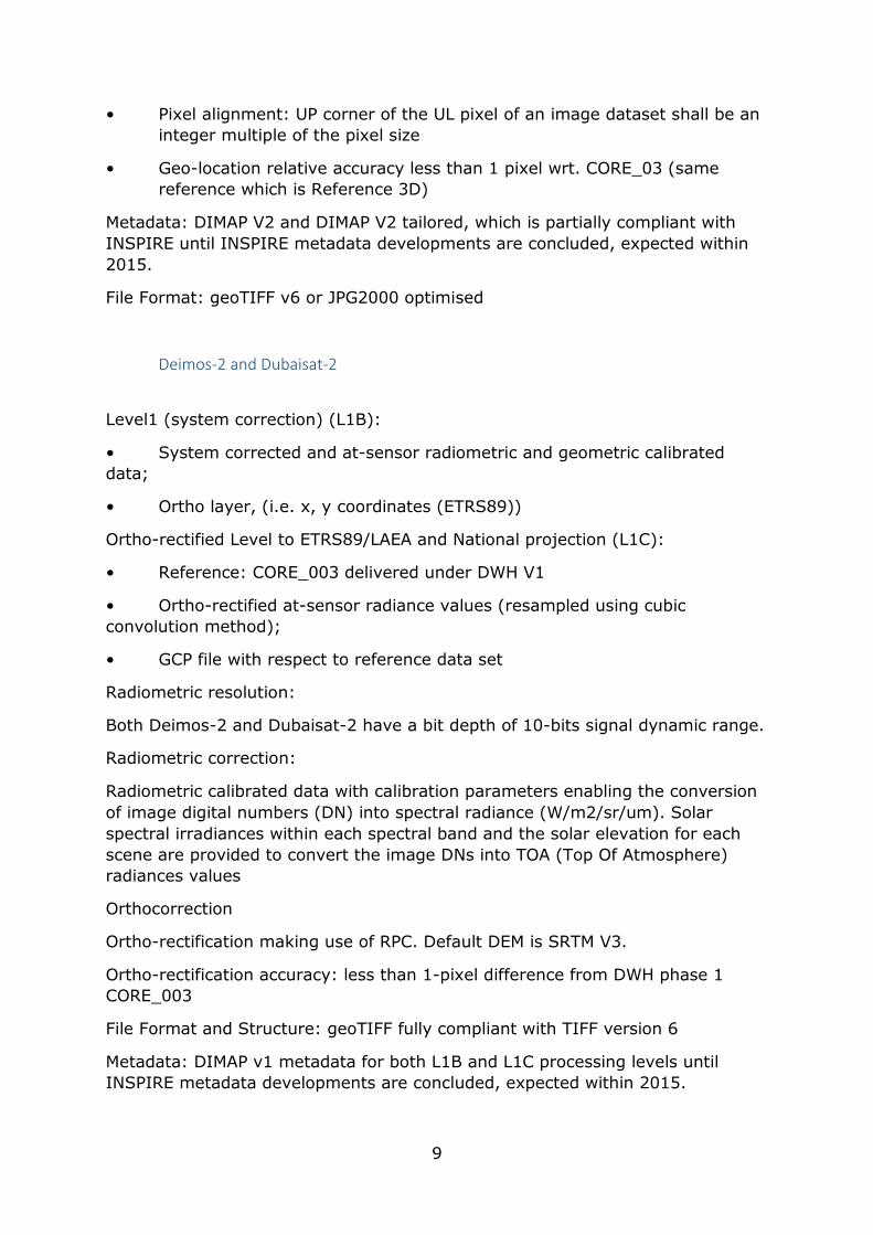
The NDVI extracted from the multispectral layer highlight clearly the vegetated

area. The values and ranges match with literature [3]. Appling thresholds, values

17

greater than 0.3 well-represent the vegetation components (Figure 10), while

negative values well describe the water presence (Figure 11).

Figure 10 - NDVI resolution 2m

Figure 11 - Water resolution 2m

Raw L3_European Mosaic space estimation

Use of the EU GHSL tool on the new VHR_IMAGE_2015

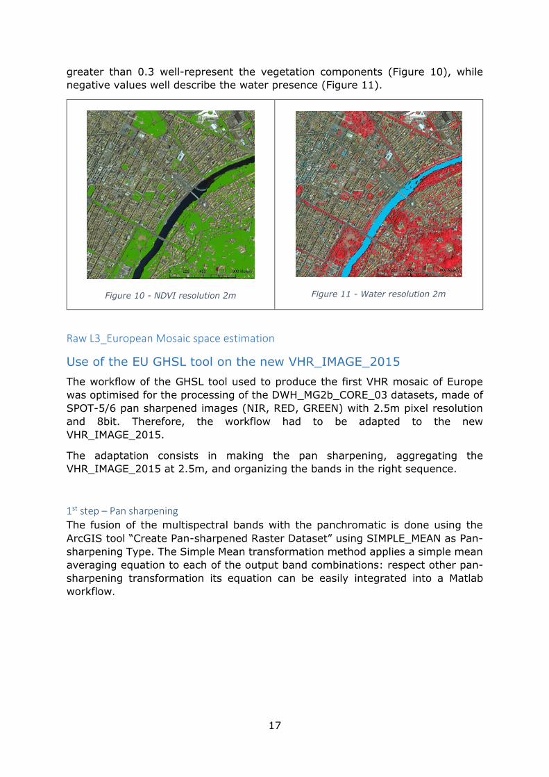
The workflow of the GHSL tool used to produce the first VHR mosaic of Europe

was optimised for the processing of the DWH_MG2b_CORE_03 datasets, made of

SPOT-5/6 pan sharpened images (NIR, RED, GREEN) with 2.5m pixel resolution

and 8bit. Therefore, the workflow had to be adapted to the new

VHR_IMAGE_2015.

The adaptation consists in making the pan sharpening, aggregating the

VHR_IMAGE_2015 at 2.5m, and organizing the bands in the right sequence.

1st step – Pan sharpening

The fusion of the multispectral bands with the panchromatic is done using the

ArcGIS tool “Create Pan-sharpened Raster Dataset” using SIMPLE_MEAN as Pan-

sharpening Type. The Simple Mean transformation method applies a simple mean

averaging equation to each of the output band combinations: respect other pan-

sharpening transformation its equation can be easily integrated into a Matlab

workflow.

18

Figure 12 - ArcGis settings Pan-sharpening

2nd step aggregation to 2.5m

The aggregation is done using the GDAL utility tool “gdalwarp” using average as

resampling operator.

gdalwarp -tr 2.5 2.5 -r average -co "COMPRESS=LZW" --config GDAL_CACHEMAX 2000

PH1A_PHR_BUN__3_20150811T103101_20150811T103104_TOU_1234_643c_psh.tif

PH1A_PHR_BUN__3_20150811T103101_20150811T103104_TOU_1234_643c_psh_2m5_average.tif

3rd step from 16 bit to 8 bit

The rescaling from 16bit to 8bit is done because the GHSL Tool contains a function

named PANTEX which accepts as input only 8bit datasets %matlab code addpath(genpath('/mnt/public/Isferea/Management/Public Tools/'));

im =

imread('PH1A_PHR_BUN__3_20150811T103101_20150811T103104_TOU_1234_643c_psh_2m5_average.tif');

geinfo =

geoiminfo('PH1A_PHR_BUN__3_20150811T103101_20150811T103104_TOU_1234_643c_psh_2m5_average.tif

');

for i = 1:4

bandi = im(:,:,i);

maxVal = mean(bandi(:));

stdval = std(single(bandi(:)),'omitnan');

im(:,:,i) = (single(im(:,:,i)) ./ (maxVal+2*stdval)) .* 255;

end

NIR = im(:,:,4);

RED = im(:,:,1);

GREEN = im(:,:,2);

imres = NIR;

imres = cat(3,imres,RED);

19

imres = cat(3,imres,GREEN);

geoimwrite(uint8(imres),'PH1A_PHR_BUN__3_20150811T103101_20150811T103104_TOU_1234_643c_psh8bi

t_matlab.tif',geinfo);

After this step, the image is ready to be processed using the GHSL tool.

The IQsHR_GHSL_V5b

The GHSL tool optimized for the European dataset is a Matlab tool named

IQsHR_GHSL_V5b. It takes as input a parameter file with all the information

needed for the processing. The parameter file used to process the sample image

over Torino is shown below.

input#NIR#string#/mnt/processing/02_REGIONAL/URBA_GHSL_EU/ver_7/VHR_IMAGE_2015/IT/60/L3_European/PH1A_PHR_BUN__3_201

50811T103101_20150811T103104_TOU_1234_643c_psh8bit_matlab.tif#1

input#GREEN#string#/mnt/processing/02_REGIONAL/URBA_GHSL_EU/ver_7/VHR_IMAGE_2015/IT/60/L3_European/PH1A_PHR_BUN__3_2

0150811T103101_20150811T103104_TOU_1234_643c_psh8bit_matlab.tif#3

input#RED#string#/mnt/processing/02_REGIONAL/URBA_GHSL_EU/ver_7/VHR_IMAGE_2015/IT/60/L3_European/PH1A_PHR_BUN__3_201

50811T103101_20150811T103104_TOU_1234_643c_psh8bit_matlab.tif#2

output#features#string#/mnt/processing/02_REGIONAL/URBA_GHSL_EU/ver_7/VHR_IMAGE_2015/IT/60/L3_European/out.tif#

output#xml#string#/mnt/processing/02_REGIONAL/URBA_GHSL_EU/ver_7/VHR_IMAGE_2015/IT/60/L3_European/out.xml#

output#mat#string#/mnt/processing/02_REGIONAL/URBA_GHSL_EU/ver_7/VHR_IMAGE_2015/IT/60/L3_European/out.mat#

param#cloudmask_folder#string#\NETAPP1\iq\process\projects\DG_2012_REGIO_GMES\cloud\VER1-0#

param#showmes#scalar#1#

param#res_out#scalar#-1#

param#res_out_type#string#box#

param#res_proc#scalar#2.5#

param#res_proc_type#string#bicubic#

param#orig_res#scalar#1#

param#Feat_mrph_lambda#vector#0,50,150,250,350,450,550,650,750,850,950,1050,1150,1250,1350,1450,1550,1650,1750,1850,1950,20

50,2150,2250,2350,2450,2550,2650,2750,2850,2950,3050,3150,3250,3350,3450,3550,3650,3750,3850,3950,4050,4150,4250,4350,4450,4

550,4650,4750,4850,4950#

param#Feat_ptx_wsize#vector#9,9#

param#Feat_tilesize#vector#3000,3000#

param#Feat_VegMfactor#scalar#0#

param#Feat_VegRescaleMin#scalar#-0.3#

param#Feat_VegRescaleMax#scalar#0.5#

param#Feat_ptxRescaleMax#scalar#1000#

param#Training_RescaleMin#scalar#0#

param#Training_rescaleMax#scalar#30#

param#Training_name#string#_sealing_v2#

param#Training_res#scalar#50#

param#Training_CloseOpenSE#scalar#4#

param#Training_areaHF#scalar#10#

param#Training_dilateradius#scalar#1#

%%param#Training_smoothradius#scalar#15#

param#Landcover_name#string#_CLC_2000_ORG#

param#Landcover_bu_off_list#vector#7,8,30,31,34,38,40,41,42,43,44#

param#Landcover_bu_list#vector#1,2,3#

param#Landcover_buscatter_list#scalar#2#

param#Landcover_water_list#vector#40,41,42,43,44#

param#Landcover_in_veg_list#vector#10,16,18,22,23,24,25,26,27,28,29#

param#Landcover_off_veg_list#vector#1,3,4,5,7,8,9,31,33,34#

param#LearnPantex_Tilesize#vector#400,400#

param#LearnPantex_PriorSmooth#vector#5,5#

param#LearnPantex_Datamax#scalar#255#

param#LearnPantex_Datamin#scalar#1#

param#LearnPantex_Nbins#scalar#256#

param#LearnPantex_Mintrsh#scalar#3#

param#LearnPantex_f_bias#vector#0,0#

param#LearnPantex_f_gain#scalar#0.9#

param#LearnPantex_smooth#vector#3,3#

param#LearnPantex_BoudZeroPrior#scalar#1#

20

param#LearnPantex_InjectApriori#scalar#1#

param#LearnPantex_InjectAprioriWeight#scalar#100#

param#LearnPantex_InjectAprioriKernel#scalar#15#

param#LearnMorpho_stdf1#scalar#-0.5#

param#LearnMorpho_stdf2#scalar#1#

param#LearnMorpho_SSLBUdomain_trsh#scalar#99#

param#LearnVegNaturalAreas#scalar#0#

param#LearnVegStdTrsh#scalar#210#

param#LearnVeg_stdf1#scalar#0#

param#LearnVeg_stdf2#scalar#2#

param#ptxClosingSize#scalar#40#

param#ptxFeatheringSize#scalar#21#

param#MorphoBuiltEnphasize#scalar#0#

param#BUMaxInnerHolePix#scalar#24000#

param#NoCPUs#scalar#8#

param#useParallelFeatureExtraction#scalar#0#

param#useParallelLearnClassification#scalar#0#

param#srid#string#3035#

param#save_intermediate_results#scalar#1#

The execution command is: /mnt/public/Isferea/Management/Public\ Tools/MATLAB_mirrored/IQ_scripts/2nd\

generation/Linux/IQsHR_GHSL_V5b/run_IQsHR_GHSL_V5b.sh /usr/local/MATLAB/MATLAB_Compiler_Runtime/v80 -F

/mnt/processing/02_REGIONAL/URBA_GHSL_EU/ver_7/VHR_IMAGE_2015/IT/60/L3_European/param.txt

The execution time of the process took 186.9138 seconds. It is much less than

the time needed to process a scene in the old DWH_MG2b_CORE_03 datasets.

The increase of speed can be attributed to the smaller size (in pixels) of the

scenes.

The result of the test on the area of Turin (Torino, 8 – Aug – 2015) (Figure 13)

looks comparable to the one done using the SPOT (Torino, 20 – Oct – 2011)

(Figure 14). No major changes in built-up are detected in the time lapse.

Torino, 20 – Oct – 2011 Torino, 8 – Aug – 2015

Figure 13 - GHSL output OLD dataset (2.5m)

Figure 14 - GHSL output NEW dataset (2.5m)

21

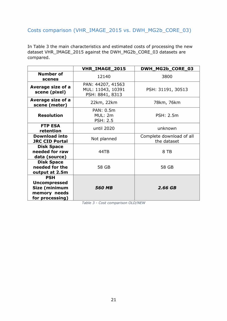
Costs comparison (VHR_IMAGE_2015 vs. DWH_MG2b_CORE_03)

In Table 3 the main characteristics and estimated costs of processing the new

dataset VHR_IMAGE_2015 against the DWH_MG2b_CORE_03 datasets are

compared.

VHR_IMAGE_2015 DWH_MG2b_CORE_03 Number of

scenes 12140 3800

Average size of a scene (pixel)

PAN: 44207, 41563

MUL: 11043, 10391 PSH: 8841, 8313

PSH: 31191, 30513

Average size of a scene (meter) 22km, 22km 78km, 76km

Resolution PAN: 0.5m MUL: 2m

PSH: 2.5

PSH: 2.5m

FTP ESA retention

until 2020 unknown

Download into JRC CID Portal

Not planned Complete download of all

the dataset

Disk Space needed for raw

data (source)

44TB 8 TB

Disk Space

needed for the output at 2.5m

58 GB 58 GB

PSH Uncompressed

Size (minimum memory needs for processing)

560 MB 2.66 GB

Table 3 - Cost comparison OLD/NEW

22

Conclusions The characteristics of this dataset offer new research opportunities. Some of them

are technical challenges related to massive processing of big data, other are

thematic research in urbanization at very high resolution, such as changes in

shape and size of settlements across time. Contrary what one might expected the

cost of processing does not seem to increase, due to an externalization of the cost

to store the raw data.

RAM size requirement

The average size in pixel of an image of the new dataset (PAN) is comparable to

the one of the old dataset, but the pan-sharpened version is much smaller. This

is a very important characteristic to be taken into consideration when processing

the files. Because the processing works at 2.5 meter, also machines with low

amount of memory can process the raw input data, or more powerful machines

can process more images simultaneously. The low memory need positively

influences cluster management. The size of a raw PSH in RAM memory is about

560MB which can easily be contained in memory in any commercial computers

nowadays.

Retention 2020

The new dataset contains much more images than the old one, and its raw weight

(raw data) on the disk is 8 times bigger than the DWH_MG2b_CORE_03. Because

it will be retained in the ESA ftp until the 2020, there is no need to download the

whole dataset, but just the image to be processed.

Time of processing

Although the estimated time needed to process the new dataset will be similar to

the old one, the number of error due to lack of memory (in concurrent operation)

will considerably be reduced thanks to their size.

Possible improvements of the algorithm

The characteristics of calibration and radiometric correction of the new dataset,

open to further improvements of the GHSL tool, which now can rely on a consistent

spectral signature across the scenes. For example, the classification of the

vegetation using the NDVI will be more precise and accurate. The algorithm to

extract the urban green will be faster because the spectral signature can be used

in place of a complex, slow learning/rescaling process that needs reference layers.

The built-up detection algorithm can take advantage of known spectral building

characteristics in its morphological operation of classification.

23

List of figures Figure 1 - Large regions map and providers ................................................ 11

Figure 2 - ftp 1st level directory structure .................................................... 11

Figure 3 - Large regions map with codes ..................................................... 12

Figure 4 – ftp 2nd level directory structure ................................................... 12

Figure 5 - ftp 3rd level directory structure .................................................... 13

Figure 6 - ftp 4th level directory structure .................................................... 13

Figure 7 - EOLiSA/GCL interface ................................................................. 14

Figure 8 - Torino false colour (resolution 2m) .............................................. 16

Figure 9 - Torino panchromatic (resolution 0.5m) ........................................ 16

Figure 10 - NDVI resolution 2m ................................................................. 17

Figure 11 - Water resolution 2m ................................................................ 17

Figure 12 - ArcGis settings Pan-sharpening ................................................. 18

Figure 13 - GHSL output OLD dataset (2.5m) .............................................. 20

Figure 14 - GHSL output NEW dataset (2.5m) ............................................. 20

List of tables Table 1- Access rights............................................................................... 15

Table 2 - Last acquisition report 15th Aug. 2016 ........................................... 16

Table 3 - Cost comparison OLD/NEW .......................................................... 21

References [1] B. Armin, D. M. Giovanni, and A. Paer, “Specifications of view services for

GMES Core_003 VHR2 coverage,” 2012.

[2] A. J. Florczyk, S. Ferri, V. Syrris, T. Kemper, M. Halkia, P. Soille, and M. Pesaresi, “A New European Settlement Map From Optical Remotely Sensed

Data,” IEEE J. Sel. Top. Appl. Earth Obs. Remote Sens., vol. 9, no. 5, pp. 1–15, 2015.

[3] J. W. and D. Herring, “Measuring Vegetation (NDVI & EVI) : Feature

Articles,” 2000.

24

LB-N

A-2

8130-E

N-N

doi:10.2788/4022

ISBN 978-92-79-62216-8