Embed Size (px)
Citation preview

University of Kentucky University of Kentucky
UKnowledge UKnowledge
Theses and Dissertations--Civil Engineering Civil Engineering
2012
AN INNOVATIVE APPROACH TO MECHANISTIC EMPIRICAL AN INNOVATIVE APPROACH TO MECHANISTIC EMPIRICAL
PAVEMENT DESIGN PAVEMENT DESIGN
Ronnie Clark Graves II University of Kentucky, [email protected]
Right click to open a feedback form in a new tab to let us know how this document benefits you. Right click to open a feedback form in a new tab to let us know how this document benefits you.
Recommended Citation Recommended Citation Graves, Ronnie Clark II, "AN INNOVATIVE APPROACH TO MECHANISTIC EMPIRICAL PAVEMENT DESIGN" (2012). Theses and Dissertations--Civil Engineering. 4. https://uknowledge.uky.edu/ce_etds/4
This Doctoral Dissertation is brought to you for free and open access by the Civil Engineering at UKnowledge. It has been accepted for inclusion in Theses and Dissertations--Civil Engineering by an authorized administrator of UKnowledge. For more information, please contact [email protected].

STUDENT AGREEMENT: STUDENT AGREEMENT:
I represent that my thesis or dissertation and abstract are my original work. Proper attribution
has been given to all outside sources. I understand that I am solely responsible for obtaining
any needed copyright permissions. I have obtained and attached hereto needed written
permission statements(s) from the owner(s) of each third-party copyrighted matter to be
included in my work, allowing electronic distribution (if such use is not permitted by the fair use
doctrine).
I hereby grant to The University of Kentucky and its agents the non-exclusive license to archive
and make accessible my work in whole or in part in all forms of media, now or hereafter known.
I agree that the document mentioned above may be made available immediately for worldwide
access unless a preapproved embargo applies.
I retain all other ownership rights to the copyright of my work. I also retain the right to use in
future works (such as articles or books) all or part of my work. I understand that I am free to
register the copyright to my work.
REVIEW, APPROVAL AND ACCEPTANCE REVIEW, APPROVAL AND ACCEPTANCE
The document mentioned above has been reviewed and accepted by the student’s advisor, on
behalf of the advisory committee, and by the Director of Graduate Studies (DGS), on behalf of
the program; we verify that this is the final, approved version of the student’s dissertation
including all changes required by the advisory committee. The undersigned agree to abide by
the statements above.
Ronnie Clark Graves II, Student
Dr. Kamyar Mahboub, Major Professor
Dr. Kamyar Mahboub, Director of Graduate Studies

AN INNOVATIVE APPROACH TO MECHANISTIC EMPIRICAL PAVEMENT DESIGN
_________________________________
DISSERTATION _________________________________
A dissertation submitted in partial fulfillment of the requirements for the degree of Doctor of Philosophy in
Civil Engineering in the College of Engineering at the University of Kentucky
By Ronnie Clark Graves II
Lexington, Kentucky
Director: Dr. Kamyar Mahboub Professor of Civil Engineering
Lexington, Kentucky
2012
Copyright © Ronnie Clark Graves II 2012

ABSTRACT OF DISSERTATION
AN INNOVATIVE APPROACH TO MECHANISTIC EMPIRICAL PAVEMENT DESIGN
The Mechanistic Empirical Pavement Design Guide (MEPDG) developed by the
National Cooperative Highway Research Program (NCHRP) project 1-37A, is a very powerful tool for the design and analysis of pavements. The designer utilizes an iterative process to select design parameters and predict performance, if the performance is not acceptable they must change design parameters until an acceptable design is achieved. The design process has more than 100 input parameters across many areas, including, climatic conditions, material properties for each layer of the pavement, and information about the truck traffic anticipated. Many of these parameters are known to have insignificant influence on the predicted performance
During the development of this procedure, input parameter sensitivity analysis varied a single input parameter while holding other parameters constant, which does not allow for the interaction between specific variables across the entire parameter space. A portion of this research identified a methodology of global sensitivity analysis of the procedure using random sampling techniques across the entire input parameter space. This analysis was used to select the most influential input parameters which could be used in a streamlined design process.
This streamlined method has been developed using Multiple Adaptive Regression Splines (MARS) to develop predictive models derived from a series of actual pavement design solutions from the design software provided by NCHRP. Two different model structures have been developed, one being a series of models which predict pavement distress (rutting, fatigue cracking, faulting and IRI), the second being a forward solution to predict a pavement thickness given a desired level of distress. These thickness prediction models could be developed for any subset of MEPDG solutions desired, such as typical designs within a given state or climatic zone. These solutions could then be modeled with the MARS process to produce am “Efficient Design Solution” of pavement thickness and performance predictions. The procedure developed has the potential to significantly improve the efficiency of pavement designers by allowing them to look at many different design scenarios prior to selecting a design for final analysis.

KEYWORDS: Mechanistic-Empirical Pavement Design, Sensitivity, Pavement Performance, Pavement Design Reliability, Thickness Design
Ronnie Clark Graves II
Student’s Signature
December 13, 2012 Date

AN INNOVATIVE APPROACH TO MECHANISTIC EMPIRICAL PAVEMENT DESIGN
By
Ronnie Clark Graves II
Dr. Kamyar Mahboub Director of Dissertation
Dr. Kamyar Mahboub Director of Graduate Studies December 13, 2012
Date
iii
TABLE OF CONTENTS
List of Tables ..................................................................................................................... v
List of Figures ................................................................................................................... vi
1.0 Background ................................................................................................................. 1
1.1 Introduction .............................................................................................................. 1
1.2 Historical Pavement Design ..................................................................................... 2
1.3 Kentucky Procedure .................................................................................................. 4
1.4 AASHTO 1993 Design Procedure ............................................................................ 4
1.5 National Cooperative Highway Research Program (NCHRP) 1-37A ..................... 5
1.6 Problem Statement .................................................................................................. 20
1.7 Significance of Research ......................................................................................... 22
2.0 Design Guide Sensitivity Analysis ........................................................................... 23
2.1 Introduction ............................................................................................................ 23
2.2 Summary of Existing Sensitivity Analysis conducted by others .............................. 27
2.3 Sampling Based Sensitivity ..................................................................................... 30
2.4 Evaluation of Sensitivity ......................................................................................... 38
3.0 Design Reliability ...................................................................................................... 53
3.1 Introduction ............................................................................................................ 53
3.2 MEPDG Reliability Concept .................................................................................. 54
3.3 Input Parameter Variability .................................................................................... 60
3.4 Monte Carlo Simulation .......................................................................................... 63
3.5 Evaluation of Distress Prediction Reliability ......................................................... 65
3.5 Summary of Results ................................................................................................. 72
4.0 Streamlined Model Development ............................................................................ 74
4.1 Introduction ............................................................................................................ 74
4.2 Selection of Modeling Methodology ....................................................................... 75
4.3 Overview of Multiple Adaptive Regression Splines Model ..................................... 77
4.4 Overview of Datasets used for Modeling ................................................................ 83
4.5 Development Model for Flexible Pavements .......................................................... 87
4.6 Development of Model for Rigid Pavements .......................................................... 96

iv
5.0 Development of Streamlined Design Process ....................................................... 105
5.1 Overview of Need for Streamlined Design Process .............................................. 105
5.2 Comparison of Actual Pavement Design Processes ............................................. 107
5.3 Overview of Streamlined Design Process Software ............................................. 111
6.0 Summary of Recommendations ............................................................................. 113
6.1 Review of information from Sensitivity Analysis .................................................. 113
6.2 Recommended Guidelines for use of Streamlined Model ..................................... 113
6.3 Recommendations for Future Research ................................................................ 115
Appendix A -- MARS Models for all Pavement Types .............................................. 117
Appendix B – User Guide for Software ...................................................................... 164
References ...................................................................................................................... 187
Vita ................................................................................................................................. 191

v
List of Tables
Table 1. Traffic and Climate Parameters .......................................................................... 12 Table 2. Asphalt Pavement Layer Parameters .................................................................. 13 Table 3. Rigid Pavement Layer Parameters ...................................................................... 14 Table 4. Granular Base and Subgrade Parameters ............................................................ 14 Table 5. General Project Parameters ................................................................................. 15 Table 6. Design Guide HMA Input Parameters ................................................................ 32 Table 7. Other Default Input Parameters .......................................................................... 32 Table 8. Average HMA Gradations from the Kentucky Transportation Cabinet ............. 36 Table 9. Statistical Results of MEPDG Performance Models (NCHRP, March 2004) .... 42 Table 10. ANOVA Results for Actual vs. Predicted Distresses ....................................... 45 Table 11. Rigid Pavement Design Parameters .................................................................. 49 Table 12. Other Rigid Pavement Default Parameters ....................................................... 50 Table 13. Coefficient of Variation of Backcalculated Moduli ......................................... 61 Table 14. Summary of HMA Input Parameters ................................................................ 63 Table 15. Comparison of 90 percent Reliability from MEPDG and Simulation Model .. 70 Table 16. Summary of Variables in the Streamlined Model ............................................ 83 Table 17. Flexible Pavement Input Variables ................................................................... 85 Table 18. Rigid Pavement Input Variables ....................................................................... 85 Table 19. Summary of Number of Design Inputs ........................................................... 105 Table 20. Summary of Pavement Design Inputs ............................................................ 107 Table 21. Typical NCHRP Process Results .................................................................... 108 Table 22. Pavement Design Results using “Efficient Design Solution” ........................ 109

vi
List of Figures Figure 1. Idealized pavement structure ............................................................................... 1 Figure 2. Comparison of existing and MEPDG design process ......................................... 7 Figure 3. Overview of NCHRP design process (NCHRP, 2004) ....................................... 8 Figure 4. Flowchart of NCHRP design process .................................................................. 9 Figure 5. Typical HMA rutting ......................................................................................... 16 Figure 6. Typical HMA fatigue cracking .......................................................................... 16 Figure 7. Typical HMA thermal (block) cracking ............................................................ 17 Figure 8. Typical PCC transverse cracking ...................................................................... 18 Figure 9. Typical PCC joint faulting ................................................................................. 18 Figure 10. Typical MEPDG design result......................................................................... 19 Figure 11. Global sensitivity analysis example ................................................................ 25 Figure 12. FHWA Vehicle classification (TMG Update 2012) ........................................ 34 Figure 13. Typical truck traffic classifications ................................................................. 35 Figure 14. Correlation Coefficients Fatigue Cracking ...................................................... 39 Figure 15. Correlation Coefficients Total Rutting ............................................................ 40 Figure 16. Correlation Coefficients for IRI ..................................................................... 40 Figure 17. Comparison of reduced model and original model, fatigue cracking ............. 43 Figure 18. Comparison of reduced model and original model, rutting ............................. 43 Figure 19. Comparison of reduced model and original model -- IRI ............................... 44 Figure 20. Correlation coefficient total rutting ................................................................. 47 Figure 21. Correlation coefficient fatigue cracking .......................................................... 47 Figure 22. Correlation coefficient IRI .............................................................................. 48 Figure 23. Correlation coefficient for PCC faulting ......................................................... 51 Figure 24. Correlation coefficient for PCC slab cracking ................................................ 51 Figure 25. Correlation coefficient for PCC IRI ................................................................ 52 Figure 26. Example of accuracy of MEPDG prediction model (Darter M. , 2007) ......... 55 Figure 27. Variable standard deviation used for reliability analysis (Darter M. , 2007) .. 57 Figure 28. Example of design reliability for given distress, (NCHRP, 2004) .................. 59 Figure 29. Example discrete normal distribution .............................................................. 64 Figure 30. Cumulative distribution of fatigue cracking .................................................... 65 Figure 31. Cumulative distribution of total rutting ........................................................... 66 Figure 32. Cumulative distribution of IRI ........................................................................ 66 Figure 33. Normal quantiles, fatigue cracking .................................................................. 67 Figure 34. Normal quantiles, total rutting ......................................................................... 68 Figure 35. Normal Quantiles, IRI ..................................................................................... 68 Figure 36. Basis function used by MARS (Hastie, Tibshirani, & Friedman, 2001) ......... 79 Figure 37. Comparison of actual IRI and MARS predicted IRI ....................................... 88 Figure 38. Comparison of total rutting with MARS predicted total rutting ..................... 89 Figure 39. Comparison of fatigue cracking with MARS predicted fatigue cracking ....... 89 Figure 40. Comparison of actual MEPDG fatigue cracking to MARS model fatigue
cracking ........................................................................................................... 90 Figure 41. Comparison of actual thickness to MARS predicted thickness – total rutting
model............................................................................................................... 93 Figure 42. Comparison of actual thickness to MARS predicted thickness—IRI model .. 94

vii
Figure 43. Comparison of actual thickness to MARS predicted thickness—fatigue cracking model ................................................................................................ 94
Figure 44. Comparison of original MEPDG thickness with MARS predicted AC thickness .......................................................................................................... 95
Figure 45. Comparison of actual MEPDG faulting with predicted MARS faulting ........ 97 Figure 46. Comparison of actual MEPDG slab cracking with predicted MARS slab
cracking ........................................................................................................... 98 Figure 47. Comparison of actual MEPDG IRI with predicted MARS IRI ....................... 98 Figure 48. Example of slab cracking model .................................................................... 99 Figure 49. Comparison of actual MEPDG thickness with MARS predicted thickness
using the slab cracking model ....................................................................... 101 Figure 50. Comparison of actual MEPDG thickness with MARS predicted thickness
using the IRI model ....................................................................................... 102 Figure 51. Comparison of actual MEPDG thickness with MARS predicted thickness
using the faulting model................................................................................ 102 Figure 52. Example of faulting model ............................................................................ 104 Figure 53. Schematic of NCHRP design/analysis process ............................................. 106 Figure 54. Comparison of MEPDG iterations with MARS model prediction, fatigue
cracking ......................................................................................................... 110 Figure 55. Comparison of MEPDG iterations with MARS model prediction, total rutting
....................................................................................................................... 110 Figure 56. Comparison of MEPDG iterations with MARS model prediction, IRI ........ 111

1
1.0 Background
1.1 Introduction
A pavement is an engineered structure designed to transmit vehicle loads to the soil or
rock subgrade below. Pavements are typically a multilayer system with the relatively
weaker materials below and progressively stronger materials above. This type of
structure leads to an economical use of available materials. Flexible pavements typically
consist of several layers starting with an unbound base such as DGA (dense-graded-
aggregate), one or more courses of asphalt bound base (Hot Mix Asphalt – HMA)
following by an asphalt riding surface. Rigid pavements consist of two layers, the
concrete slab and the bound or unbound base layer (Huang, 2004). An idealized
pavement structure is given in Figure 1.
Figure 1. Idealized pavement structure
Subgrade Material Compacted Native Soil or
Modified Materials
Unbound Material (4” – 20” thick) Crushed Aggregates
Bound Material (3” – 15” thick) Hot Mix Asphalt or Portland Cement Concrete

2
Each of these layers in a pavement structure has different properties which define
its strength and it response to changes in the environment and the passage of vehicle
loads along the roadway. For instance, Hot Mix Asphalt (HMA) is very sensitive to
changes in temperature. This change may reduce the strength of the asphalt by as much
as 60 – 70 percent during the summer months. While the subgrade materials may be
influenced by the amount of moisture which may be present. Again fluctuations of more
than 50 percent would not be uncommon as the rainfall changes throughout the year
(Ovik, Birgisson, & Newcomb, 2000).
In its simplest form the design of a pavement deals with determining the thickness
of each of the pavement layers given in Figure 1, taking into consideration their materials
and their corresponding strength, along with the amount of traffic which the roadway will
carry. Design procedures typically fall into three categories:
• Mechanistic – analysis of the engineering response to the pavement based on the
load applied, or essentially a theoretical analysis of the pavement.
• Empirical – an analysis based on experience or a detailed experiment
• Mechanistic/Empirical – a procedure which is based on theory, then has been calibrated based on observed conditions or experimental testing.
1.2 Historical Pavement Design
Pavement design in the United States has been an evolutionary process beginning
early in the 20th century. There have been many evolutions of mechanistic, empirical
and mechanistic-empirical procedures developed using a variety of road tests and in-
service pavements. The first national effort in development of a pavement design
procedure was the road test conducted by the American Association of State Highway

3
Officials (AASHO) (AASHO, 1961). This organization is now called the American
Association of State Highway and Transportation Officials (AASHTO).
This road test was conducted in Ottawa, Illinois beginning in 1958 and continuing
into 1960. The test consisted of test tracks which were built to a variety of designs,
varying the thickness of the pavement layers and the traffic loads which were applied.
Loaded military vehicles were used to apply the traffic loads; periodic inspections of the
pavement structure were conducted to measure the condition of the roadway. These
inspections included measurements of roughness, visual observations of the roadway
condition, deflection of the pavement under loadings and determination of the Pavement
Serviceability Rating (PSR) (AASHO, 1961). PSR was a measure of the overall
condition of the pavement structure as determined by a group of individuals.
There were several drawbacks to this experiment. The experiment used limited
types of construction materials. Therefore only limited information is available regarding
how material strength would affect performance of the roadway. In addition, the test
took place in a single climatic location, while it is very similar in climate to Kentucky; it
is quite different than other geographic locations across the country. Also traffic loadings
were relatively modest compared to what is seen on today highways.
The results of this road test were utilized to develop a strictly empirical design
procedure based on the observed roadway conditions and selected design parameters. It
was first published in 1972. Subsequent revisions of the design procedure were adopted
by AASHTO in 1986, 1993 and 1998 (AASHTO, 1993).

4
1.3 Kentucky Procedure
The pavement design procedure currently used by Kentucky is a
mechanistic/empirical procedure which has been developed within the state beginning in
the early 1940’s (Baker & Drake, 1949). The initial work was empirically based and was
refined though many years of evolution by monitoring the condition of in-situ pavements.
Based on these observations, modifications were made to the design procedure through
the early 1960’s. In the 1960’s work began to develop a mechanistic design procedure
based on the “limiting strain” concepts (Southgate, Deen, & Havens, 1968). These
concepts limited the amount of vertical compressive strain which was present at the top
of the subgrade layer and the amount of tensile strain at the bottom of the asphalt layer.
This procedure was calibrated with the empirical data which had been previously
observed in Kentucky. The current design procedure was developed through the late
1970’s and early 1980’s (Havens, Deen, & Southgate, 1981). It too has drawbacks similar
to the AASHTO procedure, in that it did not use different materials or provide a means to
change the design based on the availability of premium or higher strength materials.
1.4 AASHTO 1993 Design Procedure
The predominant procedure currently in use for pavement design in the United
States today is the AASHTO 1993 guide. As previously mentioned, the AASHTO 1993
guide was developed in the late 1950’s and early 1960’s, with only minimal changes to
the procedure which is utilized today.
The design procedure was based on the accelerated AASHO road test conducted
in Ottawa Illinois. This test consisted of several different test tracks of varying

5
construction types and material type at various thicknesses of constructed layers
(Portland Cement Concrete, Hot-Mix Asphalt, and Granular Materials). Loaded military
trucks were driven across these sections to simulate the traffic which is observed on
normal roadways. At periodic intervals these pavement structures were evaluated by the
research team to monitor their condition. The pavement condition was rated on a
subjective scale from 0 to 5. This scale was a measure of the “Serviceability” of the
pavement structure. The design procedure was developed based on relating this
“Serviceability” to the, basic material properties, and the accumulated traffic into an
empirical design procedure.
The design procedure introduced the concept of “Structural Number” concept for
flexible pavements which was a means to relate the overall strength of the pavement
structure. This strength could be obtained by increasing thickness of either the hot-mix
asphalt or granular base materials. Each of these materials was assigned a strength
coefficient or “Layer Coefficient” based on laboratory testing of the material strength.
The original intent was that agencies utilizing the design guide would calibrate the
material strengths to those typical to their construction practices and materials. However,
default values have traditionally been utilized routinely by many agencies. The lack of
calibration, the fact that the test occurred at a single climatic location with limited
materials all of led to the need to develop a more robust design method.
1.5 National Cooperative Highway Research Program (NCHRP) 1-37A
The AASHTO Joint Task Force on Pavements recommended in the mid 1990’s
that the existing pavement design procedure needed to be revised (NCHRP, 2004). They

6
recommended that the design guide should be a mechanistic-empirical procedure which
utilized pavement design theory with real world pavement performance. In addition a
report by the United States General Accounting Office also indicated that the design
process was outdated and should be updated (GAO, 1997). The AASHTO Joint Task
Force initiated a research project through the National Cooperative Highway Research
Program (NCHRP) which functions under the Transportation Research Board (TRB) of
the National Academy of Sciences. This project, 1-37A was initiated in 2007 with a total
cost in excess of $6,000,000; it was completed and released to the research community in
July 2004 (NCHRP, 2004). The goal of this research effort was to utilize existing
methodologies to address some of the shortcomings of the previous pavement design
guide.
The new mechanistic-empirical design procedure implements an integrated
analysis procedure for predicting pavement performance over time, accounting for the
interaction of traffic loadings, environmental factors and structural materials. In addition,
it provides a means to evaluate design input variability and reliability.
This design guide represents a major change in the way pavement structures are
designed. A general overview of both the AASHTO 1993 procedure and the NCHRP
procedure is given in Figure 2. The designer must first consider the site conditions such
as; traffic, climate, subgrade, and existing pavement condition for rehabilitation and
construction conditions.

7
AASHTO 1993 MEPDG
Inputs
Traffic
Material Strength
Performance Factors
Reliability Drainage
Output
Pavement Structure (Thickness)
Inputs
Traffic
Climate
Thickness
Material Strength/Layer
Material Thermal/Layer
Drainage
Output
Pavement Performance
Cracking Rutting Faulting
Roughness
Figure 2. Comparison of existing and MEPDG design process

8
The designer then proposes a trial design which is evaluated by the mechanistic empirical
process to determine key performance indicators such as cracking and smoothness. If the
design does not meet the desired performance criteria, it is revised and the process is
repeated as necessary. The designer has the ability to be involved in the design process
and to consider different design features and materials for the site conditions which exist.
A general schematic of the process is given in Figure 3. A more detailed flowchart is
provided in Figure 4.
Figure 3. Overview of NCHRP design process (NCHRP, 2004)

9
The design guide is structured in a hierarchical manner, in that the design inputs
may be established at one of three input levels. These levels essentially define the
amount of confidence the user has for a given input, or how this input was determined.
As an example for traffic, a Level I input might be to have detailed analysis of the
number and weight of trucks which would be specific to a particular project. Level II
might utilize very detailed analysis of the number of trucks and regional averages for
truck weights. Level III would utilize average daily traffic, an assumption for the number
of trucks based on the type of roadway, and national averages for truck weights. These
types of scenarios would be carried out for each input required. It is anticipated that the
majority of the designs will be conducted using Level II input parameters. These designs
InputsTraffic Climate Structure Design Life
Selection of Trial Design
Structural Responses (stress, strain, displacement)
Calibrated Damage-Distress ModelsDistresses Smoothness
Performance VerificationFailure criteria
Design Reliability
Design Requirements
Satisfied? No
Feasible Design
Rev
ise
trial
des
ign
Damage Accumulation with Time
Yes
Figure 4. Flowchart of NCHRP design process

10
are carried out using an integrated software program developed during the I-37A research
project.
The design process calculates stresses and strains in various locations through the
pavement structure based on the input parameters utilizing a linear elastic analysis for
flexible pavements and a finite element analysis for rigid pavements. These resulting
stresses and strains are then used to calculate the damage to the pavement structure based
on a variety of transfer functions or distress models which have been developed through
other research efforts. These transfer functions have been calibrated using more than 800
long-term pavement performance sites across the country, which has been monitored for
more than 15 years, initially through the Strategic Highway Research Program (SHRP)
and currently by the Long-Term Pavement Performance Group within the Federal
Highway Administration (FHWA). These sites were selected to provide long-term
information regarding the performance of a variety of pavement structures across the
country. A wide range of variables have been monitored through the project including,
material characterization, traffic, and observed distresses. As was previously mentioned,
these sites were utilized to calibrate the models used in the I-37A design process. It
should be noted that these models should be considered national calibration models and
were not intended to be utilized in place of local agency calibration.
This design process may be utilized to design either Hot Mix Asphalt (HMA) or
Portland Cement Concrete (PCC) pavement structures. The input variables for traffic and
climate are identical for either pavement type, while the materials and construction
related inputs may be different depending on the type of pavement being designed. Table

11
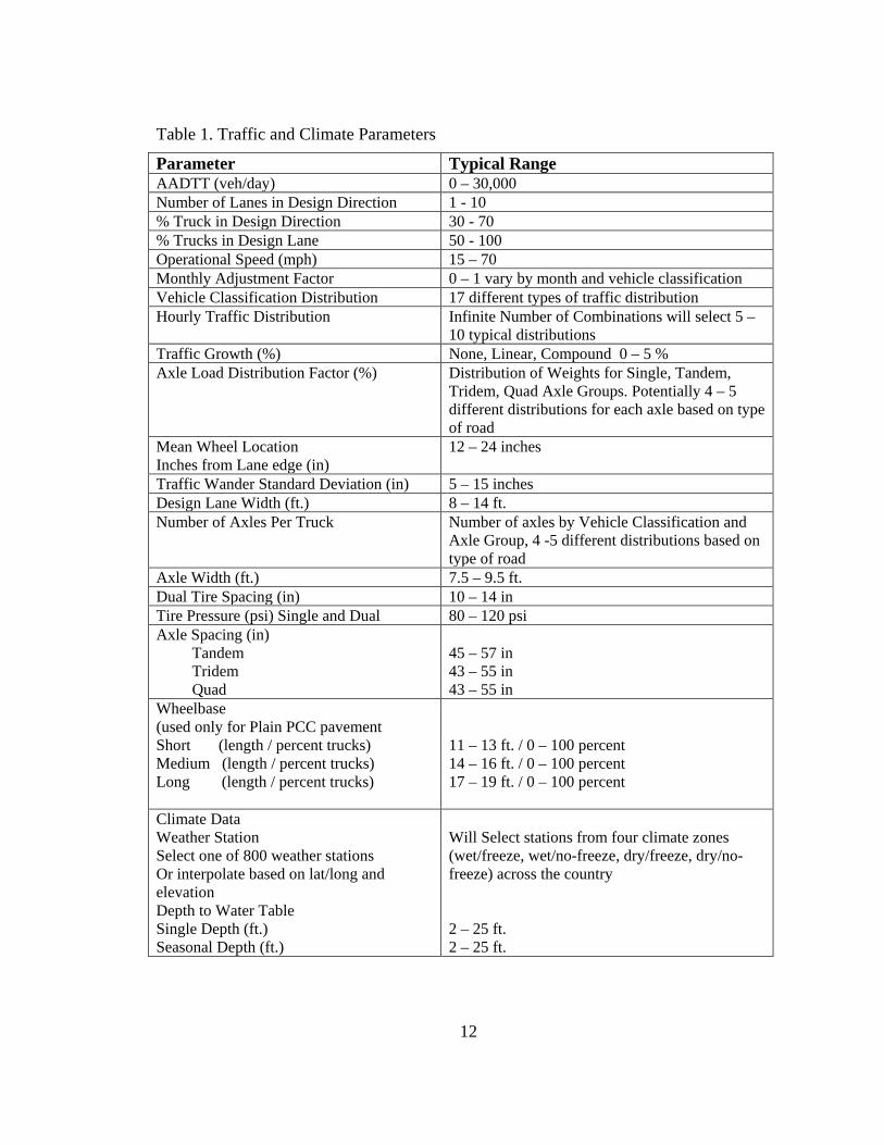
1 summarizes the traffic and climate inputs which are required. Table 2 and Table 3
provide summaries of the inputs which are required for AC and PCC pavements. Table 4
provides an overview of the required input parameters for granular base and subgrade
materials and Table 5. provides information regarding additional input parameters. The
model utilizes these design inputs to calculate the damage or distress of the pavement
structure incrementally through time on a monthly basis.
12
Table 1. Traffic and Climate Parameters
Parameter Typical Range AADTT (veh/day) 0 – 30,000 Number of Lanes in Design Direction 1 - 10 % Truck in Design Direction 30 - 70 % Trucks in Design Lane 50 - 100 Operational Speed (mph) 15 – 70 Monthly Adjustment Factor 0 – 1 vary by month and vehicle classification Vehicle Classification Distribution 17 different types of traffic distribution Hourly Traffic Distribution Infinite Number of Combinations will select 5 –
10 typical distributions Traffic Growth (%) None, Linear, Compound 0 – 5 % Axle Load Distribution Factor (%) Distribution of Weights for Single, Tandem,
Tridem, Quad Axle Groups. Potentially 4 – 5 different distributions for each axle based on type of road
Mean Wheel Location Inches from Lane edge (in)
12 – 24 inches
Traffic Wander Standard Deviation (in) 5 – 15 inches Design Lane Width (ft.) 8 – 14 ft. Number of Axles Per Truck Number of axles by Vehicle Classification and
Axle Group, 4 -5 different distributions based on type of road
Axle Width (ft.) 7.5 – 9.5 ft. Dual Tire Spacing (in) 10 – 14 in Tire Pressure (psi) Single and Dual 80 – 120 psi Axle Spacing (in) Tandem Tridem Quad
45 – 57 in 43 – 55 in 43 – 55 in
Wheelbase (used only for Plain PCC pavement Short (length / percent trucks) Medium (length / percent trucks) Long (length / percent trucks)
11 – 13 ft. / 0 – 100 percent 14 – 16 ft. / 0 – 100 percent 17 – 19 ft. / 0 – 100 percent
Climate Data Weather Station Select one of 800 weather stations Or interpolate based on lat/long and elevation Depth to Water Table Single Depth (ft.) Seasonal Depth (ft.)
Will Select stations from four climate zones (wet/freeze, wet/no-freeze, dry/freeze, dry/no-freeze) across the country 2 – 25 ft. 2 – 25 ft.

13
Table 2. Asphalt Pavement Layer Parameters
Parameter Typical Values Asphalt Layers (Separate data for each Layer)
Asphalt Mix Thickness (in) 4.5 – 18 Cumulative Percent Retained on 3/4 0 – 100 Cumulative Percent Retained on 3/8 0 – 100 Cumulative Percent Retained on #4 0 – 100 % Passing #200 0 – 100 AC Binder Grade/Strength PG 76-22 PG 64-22 Reference Temperature 60 – 80 Poisson’s Ratio 0.25 - 0.45 Effective Binder Content % 8 – 15 Air Voids % 2 – 8 Total Unit Weight (lb./ft^3) 140 - 160 Thermal Conductivity of Asphalt 0.57 - 0.77 Heat Capacity of Asphalt 0.27 – 0.47 Other Parameters Surface Shortwave absorptivity 0.75 – 0.95 Thermal Cracking Average Tensile Strength 200 – 500 Creep Test Results Creep Compliance Test Results Mix Coefficient of Thermal Contraction Mixture VMA (%) 12 – 24 Aggregate Coefficient of Thermal Contraction
4 x 10⁻⁶ – 6 x 10⁻⁶
Distress Potential (% lane area) Mean and Standard Deviation

14
Table 3. Rigid Pavement Layer Parameters
Parameter Typical Values Unit Weight 135 – 145 pcf Poisson’s Ratio 0.10 – 0.25 Coefficient of Thermal Expansion 5.5 x 10⁻⁶ – 7.5 x 10⁻⁶ Thermal Conductivity 1.0 – 1.5 Heat Capacity 0.15 – 0.40 Cementation Material Factor (lbs. /yd.) 500 - 700 Water/Cement Ratio 0.3 – 0.5 Aggregate Type Dolomite, Limestone, Granite,
Quartzite, Basalt, Synetite, Rhyolite, Chert, Gabbro
Reversible Shrinkage 40 – 60% Time to Develop 50% of ultimate Shrinkage 20 – 40 days Curing Method Curing Compound, Wet Curing Compressive Strength 3000 – 6000 psi Table 4. Granular Base and Subgrade Parameters
Parameter Typical Range Granular Materials Thickness (in) 4 – 24 Modulus (psi) (single or seasonal) 10,000 – 100,000 Coefficient of Lateral Pressure 0.4 – 0.6 Poisson’s Ratio 0.25 – 0.45 Plasticity Index 1 – 20 Percent Passing #200 0 – 20 Percent Passing #4 0 – 100 D60 (mm) 0 – 10 Compacted Unbound Material or Uncompacted Natural Stone
Select One
Subgrade Materials Modulus (psi) (single or seasonal) 10,000 – 100,000 Coefficient of Lateral Pressure 0.4 – 0.6 Poisson’s Ratio 0.25 – 0.45 Plasticity Index 1 – 20 Percent Passing #200 0 – 20 Percent Passing #4 0 – 100 D60 (mm) 0 – 10 Compacted Unbound Material or Uncompacted Natural Stone
Select One

15
Table 5. General Project Parameters
Parameter Typical Value Initial IRI in/mi 40 – 60 for AC
50 – 70 for PCC Base/Subgrade Construction Month and Yr.
Variable Through all Months and Multiple Years
Pavement Construction Month and Year Variable Through all Months and Multiple Years
Traffic Open Month and year Variable Through all Months and Multiple Years
Design Life (years) 10, 20, 30 The NCHRP process predicts the following individual distresses for HMA
pavements; Permanent deformation (rutting), fatigue cracking (both from the bottom of
the asphalt to the surface and from the top of the asphalt surface down), thermal cracking,
and roughness. Examples of rutting, fatigue cracking, and thermal cracking are presented
in Figure 5 through Figure 7.

16
Figure 5. Typical HMA rutting
Figure 6. Typical HMA fatigue cracking

17
Figure 7. Typical HMA thermal (block) cracking
For Rigid pavements (PCC Pavements), the NCHRP model predicts the following
individual distresses, faulting between the joints, top-down and bottom-up cracking, and
roughness. Examples of joint faulting and slab cracking are given in Figure 8 and
Figure 9.

18
Figure 8. Typical PCC transverse cracking
Figure 9. Typical PCC joint faulting

19
The roughness that is predicted for both flexible and rigid pavements is a model
that has been developed as a function of all of the other predicted distresses.
The designer must determine what level of distress is acceptable for his given
application and conduct a series of model runs to determine a combination of materials
and construction techniques which will meet his criteria for the given traffic level. This
predicted distress is predicted on a monthly basis for the life of the pavement design. An
example of the model results for asphalt pavement rutting for a 20-year design is given in
Figure 10
Figure 10. Typical MEPDG design result

20
1.6 Problem Statement
As was seen in the previous sections the new design process is quite complex
requiring numerous input factors dealing with traffic, climate, materials and construction.
The guide does not provide any information as to how sensitive the design models may
be to any of the required inputs. The developers of the model have only provided very
minimal evaluations as to how the model would react to changes in any input parameters,
such as thicker asphalt thicknesses have less distress for a given traffic level than do
thinner asphalt thicknesses.
In the recently completed FHWA workshop (Darter, Khazanovich, Yu, &
Mallela, 2005) on the new design process, it was stated that a sensitivity analysis is key to
the implementation of the design process. Other individuals have indicated that
evaluation of the sensitivity was a component of the guide which had not been addressed.
A full understanding of the complete sensitivity of the model to its inputs is a necessity
since some of the design inputs may require considerable expenditure of resources to
obtain values for local conditions. If it can be demonstrated that the default values of
some input variables can be utilized, then available resources can be focused on the
inputs which are most important.
The product produced during NCHRP 1-37A is a pavement analysis process,
pavement designers must use this process and them make the appropriate decisions
regarding what type of pavement should be built and the materials with which it should
be built. Existing design methodologies only allow for minimal changes in material
characteristics and once these decisions are made, the overall thickness of the pavement
structure can be determined directly. The new process is a major shift in how a pavement

21
is currently designed. In the new methodology, the designer may have the opportunity to
change many material properties which will change the overall performance of the
pavement structure; however this leads to a process which is iterative in nature instead of
a direct solution to a pavement design problem. As was mentioned in previous sections,
the designer must make assumptions regarding a potential design and available materials
and then execute the model to determine the performance of the designed pavement, if
the performance is not acceptable, additional trials must be conducted until acceptable
predicted conditions have been achieved. This could be a very cumbersome and tedious
process since there are a wide variety of input variables and it is unknown at this time
which input variable would have the largest impact on the resulting performance
prediction. The methodology is structured around an analysis tool which executed
repeatedly in search of a suitable design.
The procedure in its current form could be difficult for a highway agency to
implement and utilize on a regular basis. A streamlined, more direct utilization of the
developed model would be an invaluable tool to the pavement community. Work
completed in this research effort produces a starting point that can be then be refined by
utilizing the NCHRP procedure.
Another issue, which has not been addressed, is the calibration of the model to
local conditions. As was previously mentioned, the models which utilize the calculated
stresses and strains to determine the observed distress of the pavement structure have
been developed on a national basis. These models must be calibrated to predict the
distresses which are actually observed on a local (statewide) level. The guide does

22
provide some information as to how this would be accomplished. Guidance regarding the
local calibration of the guide is addressed in NCHRP project, NCHRP 1-40B “Local
Calibration Guidance for the Recommended Guide for Mechanistic-Empirical Design of
New and Rehabilitated Pavement Structures” (AASHTO, 2010)
1.7 Significance of Research
It is anticipated that this project will identify the key input parameters which have
the most significant impact on the pavement performance predicted by the 1-37A model.
In addition, the development of a streamlined model will expand the potential user base
of the model, by allowing those who may not have the expertise to interpret the large
array of input parameters, a more streamlined means to analyze and design pavements.
The streamlined model with its reduced set of input values will provide a starting point or
initial trial design, which can be further refined by using the full NCHRP design model.
It is intended to be a complement to the NCHRP procedure rather than a complete
replacement.

23
2.0 Design Guide Sensitivity Analysis
2.1 Introduction
Sensitivity analysis is the evaluation of how the variation in the output of a model
(numerical or otherwise) can be attributed to the input parameters of the model. The goal
of sensitivity analysis is to determine how these changes in output may affect the decision
that is made using the model results.
There are a number of techniques which can be used for evaluation of elaborate
computer models; each has its own advantages and disadvantages. Many factors are
involved in determining which method would provide the best evaluation of the model in
questions. As a whole, sensitivity analysis is used to increase the confidence in the
model and its predictions, by providing an understanding of how the model response
variables respond to changes in the inputs. Sensitivity analysis is closely linked to
uncertainty analysis which aims to quantify the overall uncertainty associated with the
response as a result of uncertainties in the model input.
Sensitivity analysis methods may be grouped into three general classes: screening
methods, local sensitivity analysis, and global sensitivity analysis (Saltelli, Chan, &
Scott, 2000). Screening methods typically are used to rank a series of input factors in
order of importance; they generally do not provide quantifiable information regarding
how much more important a given factor is than other factor. Local sensitivity analysis
concentrates on the local impact of the factors on the model; it is essentially a one-factor-
at-a-time analysis, which means one factor is varied while all others are held constant.

24
A global sensitivity analysis typically varies the input parameters across the entire
input space. Sampling based methods of uncertainty and sensitivity analysis which may
utilize Monte Carlo sampling and Latin Hyper Cube Sampling of the input parameters
have also been shown to be effective in the evaluation of complex model sensitivity and
have been utilized in a variety of applications (Helton & Davis, 2000), (Saltelli, Chan, &
Scott, 2000), (Mrawira, 1996). In this type of analysis, a sample is taken from the
distribution of each input variable and run through the model to be evaluated. The
resulting outputs of each model run are then compared to the input parameter space to
evaluate input sensitivity. A schematic of this process is given in Figure 11.

25
This process is repeated through numerous simulations using defined distributions
of the input parameters, creating a matrix of different models runs, across the full range
of input values with each run having a model result as the output. This results in a
distribution of the model output parameters. The matrix of model inputs and resulting
outputs may then be evaluated by various techniques to address the uncertainty and
sensitivity of the model to its input parameters.
A variety of methods to evaluate input sensitivity using the sampling based
process outlined above are available (Iman & Helton, 1995). These methods include
Design Model Inputs
Distributions
1-37A Design Process
Model Response
Distribution
(Cracking, Rutting,
Roughness, etc)Traffic
Material
Climate
Monte Carlo Sampling of Input Parameters
Figure 11. Global sensitivity analysis example

26
graphical measures such as scatter plots, correlation techniques such as Pearson’s and
Spearman’s correlation coefficients, regression analysis, partial correlation, and rank
transformations.
Iman and Helton, along with others have utilized the techniques of Pearson’s and
Spearman’s correlation coefficients to evaluate the global sensitivity analysis results.
These correlation coefficients provide a means to evaluate the relative sensitivity of a
given input to the output of interest. In general, a negative correlation coefficient
indicates that as the input parameters increased the output would decrease, while a
positive coefficient indicates that at the input parameter increases the output increases.
Pearson’s correlation coefficient makes the assumption that the relationship between the
input and output is linear, while Spearman’s rank correlation converts the actual raw
values to ranks and does not require the assumption of linearity (Saltelli, Tarantola, &
Ratto, 2004). Since the design guide is a complex system and all the relationships may
not be linear, both correlation techniques were utilized to evaluate the sensitivity of the
input variables.
A sampling based methodology has been developed to evaluate various inputs of
the design guide (Graves & Mahboub, 2006). This analysis utilized a sampling based
technique where the entire input parameter space of selected input variables is sampled.
The resulting samples are then used to create a matrix of design scenarios which may
then be run through the NCHRP MEPDG software. The NCHRP MEPDG software will
then predict the various performance parameters (cracking, rutting, faulting and
rideability) of each design scenario. These performance outputs and the corresponding

27
input parameters may then be analyzed to evaluate the sensitivity of each input parameter
with respect to each predicted distress.
Once the significant parameters have been determined, appropriate default values
may be assigned to the remaining input variables, thus streamlining the design process.
In addition, a better understanding of the sensitivity of the input parameters will allow
designers to focus attention on the collection of appropriate data during the local
calibration process. This understanding will permit the best use of available resources in
the collection of the historical data on given projects which are used for calibration.
Attention may be focused only on the parameters which have the most significant effect
on the predicted performance. Information relating to these sensitivity analysis results
will be included in later chapters.
2.2 Summary of Existing Sensitivity Analysis conducted by others
A variety of sensitivity analyses have been completed by others to try and better
understand the influential input parameters of the process. All of these sensitivity
analyses have utilized the one-factor-at-a-time method; where a single parameter of
interest is changed while all others remain constant. This is generally referred to as local
sensitivity analysis (Helton, 2004).
A number of studies have been completed in recent years to address the local
sensitivity of the MEPDG process. These studies have evaluated various aspects of
granular base material properties and thickness, HMA materials and thickness, PCC
thickness and materials, and traffic parameters.

28
Two studies examined sensitivity of the predicted flexible pavement distresses
based on the variation of input parameters. In each case, a base pavement structure has
been selected and then a variety of parameters have then been varied one-at-a-time to
evaluate sensitivity. Predicted performance of each range of variables compared to the
base-case scenario. The first study by Lee and Hall (2004) looked at the following
parameters: Poisson’s ratio, surface shortwave absorptive, heat capacity, thermal
conductivity, air voids, binder grade, total unit weight, effective binder content. Two
different asphalt mixture sizes were evaluated; 0.5-inch and 1.0-inch size maximum
aggregate. In addition, four typical HMA gradations obtained from sources within
Arkansas were utilized. Their results indicated that for surface-down cracking, only air
voids and effective binder content for 0.5-inch mixes had a significant impact on
performance. For bottom-up damage, air voids and effective binder content for both mix
sizes were found to be significant, no significant input variable was found for rutting and
only air voids and effective binder content for 0.5-inch mixes was found to be significant
for IRI. It should be noted that these studies were for a single traffic level, subgrade
strength and climatic location.
The second study was conducted as part of the development of the MEPDG
design process at the University of Arizona, by El-Basyouny and Witczak (2004). This
study focused on the sensitivity of the following: bottom-up fatigue cracking, top-down
fatigue cracking and permanent deformation. This study was again a one-factor-at-a-time
analysis where all parameters remained constant with the exception of the parameters of
interest.

29
This study in general evaluated the influence of the following factors on the
resulting prediction of fatigue cracking and longitudinal cracking:
AC Stiffness – Thin Pavements AC Stiffness – Thick Pavements AC Thickness Subgrade Modulus AC Mix Air Voids Asphalt Content Depth to GWT Traffic Volume Traffic Speed Traffic Analysis Level (Level 1, 2, 3) MAAT (Mean Annual Air Temp.) Depth to Bedrock
This study identified the general relationship between each of these inputs and the
resulting outputs, while generally all other input parameters remained constant. It was
found that subgrade stiffness and traffic generally are influential in the prediction of
performance, while some of the other parameters have varying degrees of significance.
A study by Bracher and Papagiannakis (2004), evaluated the potential sensitivity
of the various hierarchal levels and sampling schemes for the design guide traffic inputs.
These hierarchal levels deal with the source of traffic data which is utilized in the design,
site specific WIM, classification, volume, etc. or, regional and national average values.
As would be expected, it was illustrated that the variability of traffic data may have a
significant impact on the predicted performance of the pavement system. It illustrated
that regional WIM data will generally provide designs which would overestimate the base
case (continuous site specific data) by less than 20 percent.
A recent study by Masad and Little (2004) indicated that base modulus and
thickness have significant influence on the IRI and longitudinal cracking. The influence
of these properties on fatigue cracking is approximately half of the influence of the
30
properties on longitudinal cracking. It also stated that the granular base material
properties did not seem to have an influence on permanent deformation of the pavement.
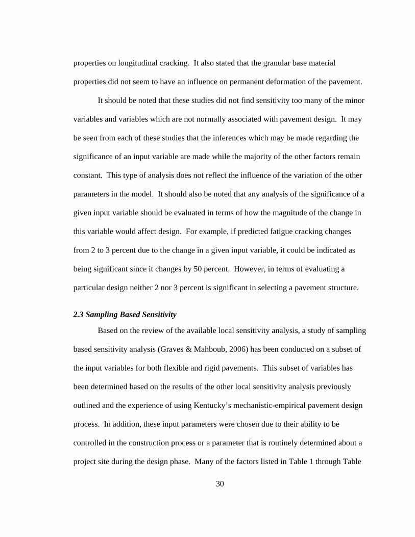
It should be noted that these studies did not find sensitivity too many of the minor
variables and variables which are not normally associated with pavement design. It may
be seen from each of these studies that the inferences which may be made regarding the
significance of an input variable are made while the majority of the other factors remain
constant. This type of analysis does not reflect the influence of the variation of the other
parameters in the model. It should also be noted that any analysis of the significance of a
given input variable should be evaluated in terms of how the magnitude of the change in
this variable would affect design. For example, if predicted fatigue cracking changes
from 2 to 3 percent due to the change in a given input variable, it could be indicated as
being significant since it changes by 50 percent. However, in terms of evaluating a
particular design neither 2 nor 3 percent is significant in selecting a pavement structure.
2.3 Sampling Based Sensitivity
Based on the review of the available local sensitivity analysis, a study of sampling
based sensitivity analysis (Graves & Mahboub, 2006) has been conducted on a subset of
the input variables for both flexible and rigid pavements. This subset of variables has
been determined based on the results of the other local sensitivity analysis previously
outlined and the experience of using Kentucky’s mechanistic-empirical pavement design
process. In addition, these input parameters were chosen due to their ability to be
controlled in the construction process or a parameter that is routinely determined about a
project site during the design phase. Many of the factors listed in Table 1 through Table

31
5 are not routinely measured as part of a pavement construction process. Some of these
parameters do not have standardized testing procedures developed and were included to
allow for future enhancements of the design methodology. The results of the design
process may be sensitive to some of these input parameters, however, since they are not
readily available at the time of design; they were not included in this analysis.
Flexible Pavement Sensitivity This initial study for flexible pavement structure focused on the eight individual input
parameters outlined below:
• Average Annual Daily Truck Traffic (AADTT) • Truck Traffic Classification (TTC) • Hot Mix Asphalt (HMA) Thickness • Subgrade Strength (characterized by CBR) • Nominal HMA Base Size • Asphalt Content (AC) Binder Grade (standard grade and “bumped” grade for
improved performance) • Climate Zone • Construction Month
The individual values which were varied and utilized in the study are given in Table 6.
Table 7 provides information on the default values utilized from the design guide for
other input parameters.

32
Table 6. Design Guide HMA Input Parameters
AADTT
Truck Traffic
Classification
Nominal HMA
Thickness (in)
Subgrade CBR
Nominal HMA Base Aggregate
Size (in)
Climate Zone
Construction Month
100 1 5 2 0.75 Cheyenne Jan. 500 4 6 4 1.0 Phoenix April
1,000 6 7 6 1.5 Lexington July 2,000 12 8 8 Birmingham Oct. 4,000 9 10 6,000 10 8,000 11
10,000 12 15,000 13 25,000 14
Table 7. Other Default Input Parameters Traffic Inputs Software Defaults were utilized with the
exception of AADTT and TTC Climate Inputs Water Table depth was assumed to be 20 feet
for all design sections. Individual weather stations in the cities provided in Table 3 were used for generation of the climate files
Structure Inputs Drainage and Surface Properties HMA Layers Granular Layer Subgrade
Software Defaults were utilized Software Defaults were utilized with the exception of the items given in Table 4 Thickness = 8.0 inches, Modulus = 40,000 psi All other parameters were software defaults based on base type Subgrade CBR varied as stated in Table 3, all other parameters defined by software based on CL Soil Classification

33
A brief discussion of each parameter is given below. AADTT were selected across a
range from 100 to 25,000 trucks per day. This range would represent typical traffic
levels what would be expected on most highways. The TTC categories were selected
from the default vehicle classification distributions provided in the design guide software.
These distributions would represent the typical ranges which would be expected for
roadways which have a predominance of single-trailer trucks. A summary of the types of
vehicles which are classified in each vehicle type are given in Figure 12. The
distributions used in this analysis are illustrated graphically in Figure 13.
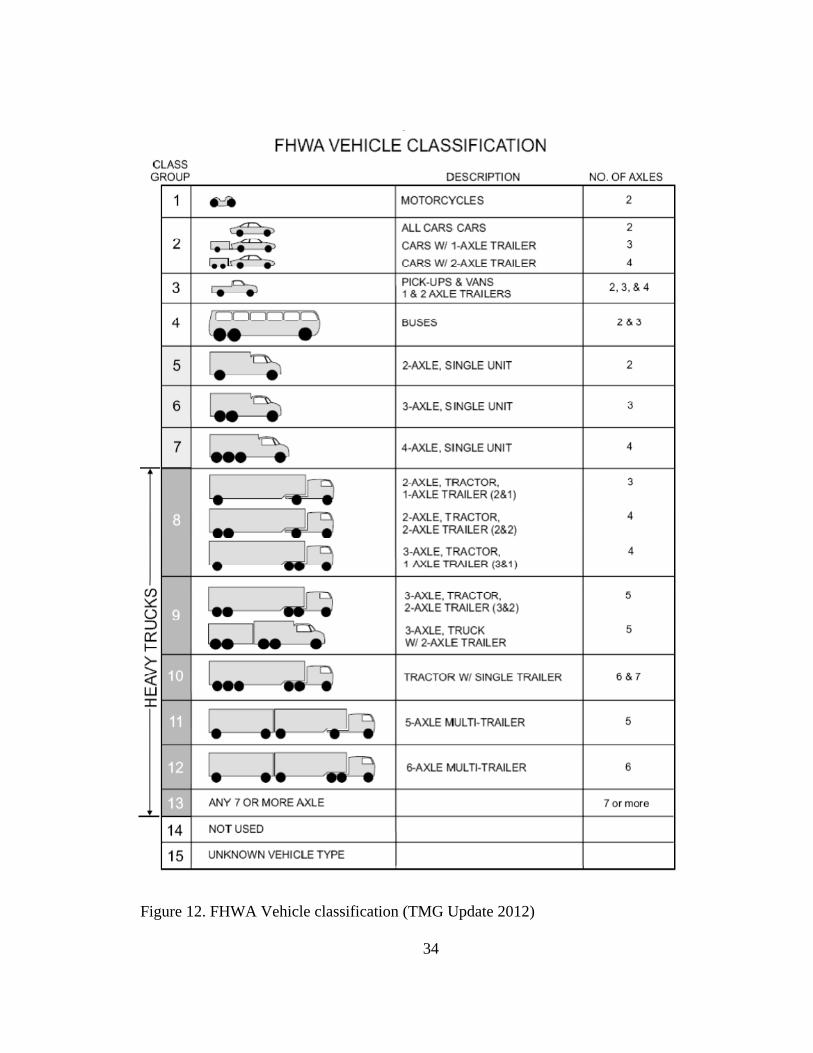
34
Figure 12. FHWA Vehicle classification (TMG Update 2012)

35
Figure 13. Typical truck traffic classifications
For the HMA layers, a thickness of 1.5-iinches was selected for all surface
mixtures. For Thicknesses greater than 6.5 inches the HMA base layers were separated
into two layers (NCHRP, 2011) , due to anomalies which have been discovered in the
design software for thickness greater than 9 inches, these anomalies produced
inconsistent results if the total thickness remained in a single layer.
The subgrade strength was varied across a range from California Bearing Ratio
(CBR) of, 2 to 10 for a CL soil type. The California Bearing Ratio is a laboratory test
method used to measure the load carrying capacity of subgrade soils and granular bases.
All other soil parameters were set to the defaults provided by the design software based
on the type of soil selected.
0
10
20
30
40
50
60
70
4 5 6 7 8 9 10 11 12 13
Vehicle Type
Perc
ent o
f Tra
ffic
Stre
am (%
)
1 4 6 12
Truck Traffic Category

36
Three HMA base nominal aggregate sizes were selected for trials in this study as
follows: 0.75, 1.0, and 1.5-inch these represent the typical designs utilized throughout
the asphalt industry. The gradations and volumetric parameters (density, air voids,
asphalt content, etc.) for these mixtures are given in Table 8. They were selected from
typical mixtures currently utilized in Kentucky. A 0.5-inch top size aggregate surface
course was utilized for each design section, the material properties for this mix are also
provided in Table 8.
Table 8. Average HMA Gradations from the Kentucky Transportation Cabinet
Mix Size (in)
VMA (%)
Unit Weight lb./ft3
Air Voids (%)
Effective Binder
(%)
% Retained
3/4-in Sieve
% Retained
3/8-in Sieve
% Retained
No. 4 Sieve
% Passing # 200
0.75 13.4 150.7 6.3 7.3 4.7 29.7 59.4 5.0
1.0 12.9 151.3 6.7 6.3 13.7 36.9 64.9 4.7
1.5 12.3 152.3 6.5 5.9 23.8 49.4 70.1 4.2
0.5 surface 15.4 149.0 7.0 8.4 0.0 13.1 40.6 5.2
A performance graded (PG) binder of PG 64-22 indicates that the average seven-day
maximum pavement temperature would be 64° C and the minimum pavement design
temperature likely to be experienced would be -22° C. When using performance graded
binders, the practice of “bumping” the binder grade refers to increasing the high
temperature component of the grading to a higher level to compensate for slower traffic
speeds or higher traffic volumes. The practice of “bumping” the Superpave binder
(KYTC, 2009) grade for the upper layers of the pavement structure was also evaluated.

37
For this analysis, the “bumped” grade was selected as two high temperature grades above
the default determined for the climatic location discussed below.
Four different climatic locations were selected across the country, which generally
represent the four climatic zones (wet - no freeze, wet - freeze, dry – no freeze, and dry -
freeze) outlined during the Strategic Highway Research Program (SHRP), (Smith, 1993),
PG binder grades for these locations were determined using the LTTP Bind software
version 2.1 (FHWA, 1999). These locations along with their default PG grade and
“bumped” grade are as follows:
• Lexington, KY (PG 64-22, PG 76-22)
• Birmingham, AL (PG 64-16, PG 76-16)
• Cheyenne, WY (PG 58-28, PG 70-28)
• Phoenix, AZ (PG 70-22, PG 82-10)
The month of construction was also varied across each of the seasons of the year,
January, April, July, and October. Each of these inputs was assigned a discrete uniform
distribution across the range of values indicated in Table 6..
These distributions were then sampled using a Monte Carlo sampling routine
using SIMLAB (SIMLAB 2006) to produce different design scenarios covering the
complete range of the input parameter space. The number of samples required for this
type of analysis is generally in the range from 8 to 10 times the number of input variables
(Saltelli, Tarantola, & Ratto, 2004). The remaining variables necessary to evaluate the
design were assigned default values based on the MEPDG software. These scenarios
were then processed through the MEPDG software to produce a matrix of outputs for the

38
following distresses: longitudinal cracking, fatigue cracking, HMA rutting, total rutting,
and IRI.
These distresses were summarized at the 20-year level for use in the sensitivity
analysis. The matrix of outputs and their corresponding matrix of input variables are then
used to evaluate the sensitivity of the design guide to the input parameters varied in the
sampling process.
2.4 Evaluation of Sensitivity
The analysis of input sensitivity was accomplished by determining the Pearson’s
Correlation Coefficient and the Spearman’s Rank Correlation Coefficient for the
relationship between the input parameters and the resulting output. To aid in evaluating
the sensitivity of each output with respect to the input parameters, “Tornado” charts were
produced for each output parameter. These charts illustrate the Pearson’s and
Spearman’s coefficients for each input parameter being studied. These results are given
in Figure 14 through Figure 16. The figures show that input parameters may have higher
or lower correlation coefficients depending on the output which is being analyzed.
Correlations marked with an “” are significant at the 95% confidence level. This
statistic along with the relative ranking of the individual input parameters was used to
evaluate the input parameters which have the least significance.
Figure 14 illustrates that fatigue cracking is significantly related to HMA
thickness, subgrade strength and AADTT, while the other parameters are somewhat less
significant. It should be noted that AADTT and HMA thickness indicate a much stronger
relationship than the other variables. For total rutting; AADTT, HMA thickness,

39
subgrade, and binder grade “bump” appear to be the most significant factors, with
AADTT again being the predominant factor. For IRI several factors appear to exhibit
influence and thus may be deemed significant; however, it should be noted that in the
MEPDG design guide, the IRI determined as a function of all the other accumulated
distresses. This fact would tend to lead to the results which are shown in Figure 16,
which indicates that several of the factors which have been discussed have significant
influence, with the exception of nominal base size and binder grade “bump”? In general
AADTT, AC thickness, climate zone and subgrade strength have large influences across
all output parameters, while the remaining variables exhibit varying degrees of influence.
Alligator Cracking
-0.8 -0.6 -0.4 -0.2 0 0.2 0.4 0.6 0.8
AADTT
AC Thickness
Base Size
Binder Grade
Climate Zone
Season
Subgrade
TTC
Inpu
t Par
amet
er
Correlation Coefficient
Pearson Spearmen
Significant at 95% Confidence Level
Figure 14. Correlation Coefficients Fatigue Cracking

40
Figure 15. Correlation Coefficients Total Rutting
Figure 16. Correlation Coefficients for IRI
IRI
-0.4 -0.3 -0.2 -0.1 0 0.1 0.2 0.3
AADTT
AC Thickness
Base Size
Binder Grade
Climate Zone
Season
Subgrade
TTC
Inpu
t Par
amet
er
Correlation Coefficient
Pearson Spearmen
Significant at 95% Confidence Level
Total Rutting
-0.4 -0.2 0 0.2 0.4 0.6 0.8 1
AADTT
AC Thickness
Base Size
Binder Grade
Climate Zone
Season
Subgrade
TTC
Inpu
t Par
amet
er
Correlation Coefficient
Pearson Spearmen
Significant at 95% Confidence Level

41
It would appear that the resulting outputs are least sensitive to construction
month, binder grade “bump”, TTC, climate zone, and nominal base size. Utilizing some
type of default value for these inputs may provide satisfactory results in prediction of the
output performance. Based on this analysis, default values for binder grade (no binder
grade “bump”), TTC, nominal base size and construction month were selected as follows:
• Binder Grade (default based on climate zone, no “bump” in grade)
Lexington, KY PG 64-22 • Construction Month: June
• Truck Traffic Classification (TTC): 6
• Nominal Base Size 1.0-inch (25 mm)
To address the feasibility of using these default input parameters, a sample of
design scenarios were obtained from the original group of used in the sensitivity
analysis. These design scenarios were selected so that they contained none of the default
input values outlined above (binder grade bump, construction month, TTC, or nominal
base size). Therefore in each case the original values for these parameters were replaced
by the default values. The MEPDG was then run using this reduced set of parameters and
then run again using the original parameters. The results from these two different
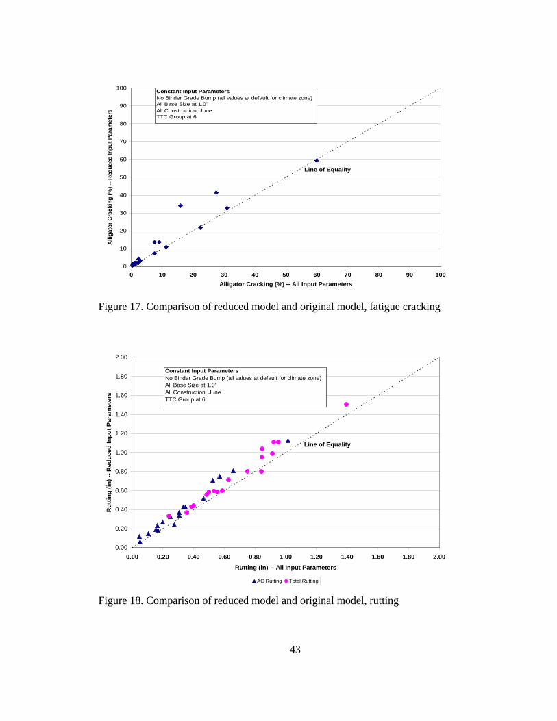
software runs were then compared. A summary of these results is shown in Figure 17
through Figure 19. These figures that the predicted distresses using the reduced set of
parameters (default values) correlates very well with the original model which included
specific inputs for each input.
42
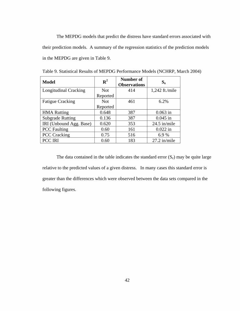
The MEPDG models that predict the distress have standard errors associated with
their prediction models. A summary of the regression statistics of the prediction models
in the MEPDG are given in Table 9.
Table 9. Statistical Results of MEPDG Performance Models (NCHRP, March 2004)
Model R2 Number of Observations Se
Longitudinal Cracking Not Reported
414 1,242 ft./mile
Fatigue Cracking Not Reported
461 6.2%
HMA Rutting 0.648 387 0.063 in Subgrade Rutting 0.136 387 0.045 in IRI (Unbound Agg. Base) 0.620 353 24.5 in/mile PCC Faulting 0.60 161 0.022 in PCC Cracking 0.75 516 6.9 % PCC IRI 0.60 183 27.2 in/mile
The data contained in the table indicates the standard error (Se) may be quite large
relative to the predicted values of a given distress. In many cases this standard error is
greater than the differences which were observed between the data sets compared in the
following figures.
43
Figure 17. Comparison of reduced model and original model, fatigue cracking
Figure 18. Comparison of reduced model and original model, rutting
0
10
20
30
40
50
60
70
80
90
100
0 10 20 30 40 50 60 70 80 90 100Alligator Cracking (%) -- All Input Parameters
Allig
ator
Cra
ckin
g (%
) -- R
educ
ed In
put P
aram
eter
s
Line of Equality
Constant Input ParametersNo Binder Grade Bump (all values at default for climate zone)All Base Size at 1.0"All Construction, JuneTTC Group at 6
0.00
0.20
0.40
0.60
0.80
1.00
1.20
1.40
1.60
1.80
2.00
0.00 0.20 0.40 0.60 0.80 1.00 1.20 1.40 1.60 1.80 2.00Rutting (in) -- All Input Parameters
Rut
ting
(in) -
- Red
uced
Inpu
t Par
amet
ers
AC Rutting Total Rutting
Line of Equality
Constant Input ParametersNo Binder Grade Bump (all values at default for climate zone)All Base Size at 1.0"All Construction, JuneTTC Group at 6

44
Figure 19. Comparison of reduced model and original model -- IRI
It is also interesting to note that in Figure 18 there is not a significant change in
the predicted rutting when the “bumped” binder grade is not utilized.
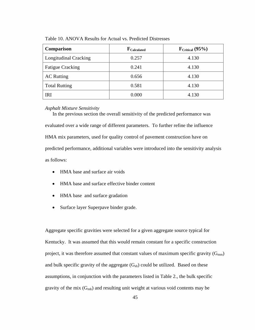
As a means to evaluate these comparisons a single factor ANOVA was conducted
between the results of the reduced parameter set and the complete input parameter set.
The ANOVA results indicated that at the 95% confidence level there is no significant
difference between the results. The ANOVA results are contained in Table 10.
50.00
60.00
70.00
80.00
90.00
100.00
110.00
120.00
50.00 60.00 70.00 80.00 90.00 100.00 110.00 120.00IRI (in/mile) -- All Input Parameters
IRI (
in/m
ile) -
- Red
uced
Inpu
t Par
amet
ers
Line of Equality
Constant Input ParametersNo Binder Grade Bump (all values at default for climate zone)All Base Size at 1.0"All Construction, JuneTTC Group at 6
45
Table 10. ANOVA Results for Actual vs. Predicted Distresses
Comparison FCalculated FCritical (95%)
Longitudinal Cracking 0.257 4.130
Fatigue Cracking 0.241 4.130
AC Rutting 0.656 4.130
Total Rutting 0.581 4.130
IRI 0.000 4.130 Asphalt Mixture Sensitivity
In the previous section the overall sensitivity of the predicted performance was
evaluated over a wide range of different parameters. To further refine the influence
HMA mix parameters, used for quality control of pavement construction have on
predicted performance, additional variables were introduced into the sensitivity analysis
as follows:
• HMA base and surface air voids
• HMA base and surface effective binder content
• HMA base and surface gradation
• Surface layer Superpave binder grade.
Aggregate specific gravities were selected for a given aggregate source typical for
Kentucky. It was assumed that this would remain constant for a specific construction
project, it was therefore assumed that constant values of maximum specific gravity (Gmm)
and bulk specific gravity of the aggregate (Gsb) could be utilized. Based on these
assumptions, in conjunction with the parameters listed in Table 2., the bulk specific
gravity of the mix (Gmb) and resulting unit weight at various void contents may be

46
determined. In addition, once the Gmb is known, the mixture voids in the mineral
aggregate (VMA) may then be calculated for each Gmb and asphalt content. Once the
VMA is known, it may be used in conjunction with air voids to determine the effective
binder content (by volume) used in Level 3 of the MEPDG software. Therefore, the
properties are linked together to provide realistic information regarding the mix instead of
just varying each parameter across a range independently. These linked properties
provide effective binder contents that range from 9.8 to 11 percent, and unit weights
ranging from 137 to148 lbs. /ft3, depending upon it being a surface mix or base mix.
The analysis of the HMA mixture inputs sensitivity was accomplished by
determining the Pearson’s Correlation Coefficient and the Spearman’s Rank Correlation
Coefficient for the relationship between the input parameters and the resulting output. To
aid in evaluating the sensitivity of each output with respect to the input parameters,
“Tornado” charts were produced for each output parameter. These charts illustrate the
Pearson’s and Spearman’s coefficients for each input parameter being studied. These
results are given in Figure 20 through Figure 22. These figures show that input
parameters may have higher or lower correlation coefficients depending on the output
which is being analyzed.

47
Figure 20. Correlation coefficient total rutting
Figure 21. Correlation coefficient fatigue cracking
-0.6 -0.4 -0.2 0 0.2 0.4 0.6
Surface Air Voids
Surface Effective AC (vol)
Surface Unit Weight
Surface Gradation
Base Air Voids
Base Effective AC (vol)
Base Unit Weight
Base Gradation
Binder Grade Bump
Alligator Cracking
Pearson Spearman
-1 -0.8 -0.6 -0.4 -0.2 0 0.2 0.4 0.6
Surface Air Voids
Surface Effective AC (vol)
Surface Unit Weight
Surface Gradation
Base Air Voids
Base Effective AC (vol)
Base Unit Weight
Base Gradation
Binder Grade Bump
Total Rutting
Pearson Spearman

48
Figure 22. Correlation coefficient IRI
Based on the results of these sensitivity analysis and experience in Kentucky’s
mechanistic-empirical pavement design procedure, a subset of variables have been
selected which represent typical pavement design parameters. It has been seen from this
analysis that various hot-mix-asphalt (HMA) mixture parameters (void content, asphalt
content, and etc.) do have some impact on performance. However, these are parameters
which are used as part of typical construction quality control, to insure minimum
standards are met. The final mixture parameters utilized through the remainder of this
study are based on specific minimum standards, which lead to more conservative designs.
-1 -0.8 -0.6 -0.4 -0.2 0 0.2 0.4 0.6 0.8
Surface Air Voids
Surface Effective AC (vol)
Surface Unit Weight
Surface Gradation
Base Air Voids
Base Effective AC (vol)
Base Unit Weight
Base Gradation
Binder Grade Bump
IRI
Pearson Spearman

49
Rigid Pavement Sensitivity The sensitivity analysis of for rigid pavements (PCC Pavements) has focused on
the following seven parameters; Average Annual Daily Truck Traffic (AADTT), PCC
Thickness, PCC Strength, subgrade strength, granular base thickness, and granular base
strength.
The individual values which were varied and used in the study are given in Table
11. Table 12 provides information on the default values chosen from the design guide for
other input parameters.
Table 11. Rigid Pavement Design Parameters
AADTT
Portland Cement
Concrete Thickness
(in)
Portland Cement
Concrete Strength
–Modulus
of Rupture
(psi)
Subgrade Strength
(psi)
Granular Base
Thickness (in.)
Granular Base
Strength (psi)
100 6 500 8,000 6 20,000 500 7 600 10,000 8 30,000
1,000 8 700 13,000 10 40,000 2,000 9 800 16,000 12 4,000 10 6,000 11 8,000 12
10,000 13 15,000 14 25,000

50
Table 12. Other Rigid Pavement Default Parameters
Traffic Inputs Software Defaults were utilized with the exception of AADTT and TTC
Climate Inputs Water Table depth was assumed to be 20 feet for all design sections. Individual weather stations in the cities provided in Table 3. were used for generation of the climate files
Structure Inputs Drainage and Surface Properties Portland Cement Concrete Layers Granular Layer Subgrade
Software Defaults were utilized Software Defaults were utilized with the exception of the items given in Table 1. Software Defaults with the exception of values given in Table 11. All other parameters were software defaults based on base type Subgrade CBR varied as stated in Table 3., all other parameters defined by software based on CL Soil Classification
The analysis of the PCC pavement structures was accomplished by determining
the Pearson’s Correlation Coefficient and the Spearman’s Rank Correlation Coefficient
for the relationship between the input parameters and the resulting output for a random
sampling of the input space identified in Table 11. To aid in evaluating the sensitivity of
each output with respect to the input parameters, “Tornado” charts were produced for
each output parameter. These charts illustrate the Pearson’s and Spearman’s coefficients
for each input parameter being studied. These results are given in Figure 23 through
Figure 25.

51
Figure 23. Correlation coefficient for PCC faulting
Figure 24. Correlation coefficient for PCC slab cracking
-1 -0.8 -0.6 -0.4 -0.2 0 0.2 0.4 0.6 0.8 1
AADTT
PCC Thickness
Dowel Bar Diameter
PCC Flexural Strength
Subgrade Modulus
DGA Thickness
DGA Modulus
Correlation Coefficient
Faulting
Pearson Spearman
-1 -0.8 -0.6 -0.4 -0.2 0 0.2 0.4 0.6 0.8 1
PCC Thickness
AADTT
PCC Flexural Strength
DGA Modulus
DGA Thickness
Subgrade Modulus
Dowel Bar Diameter
Correlation Coefficient
Slab Cracking
Pearson Spearman
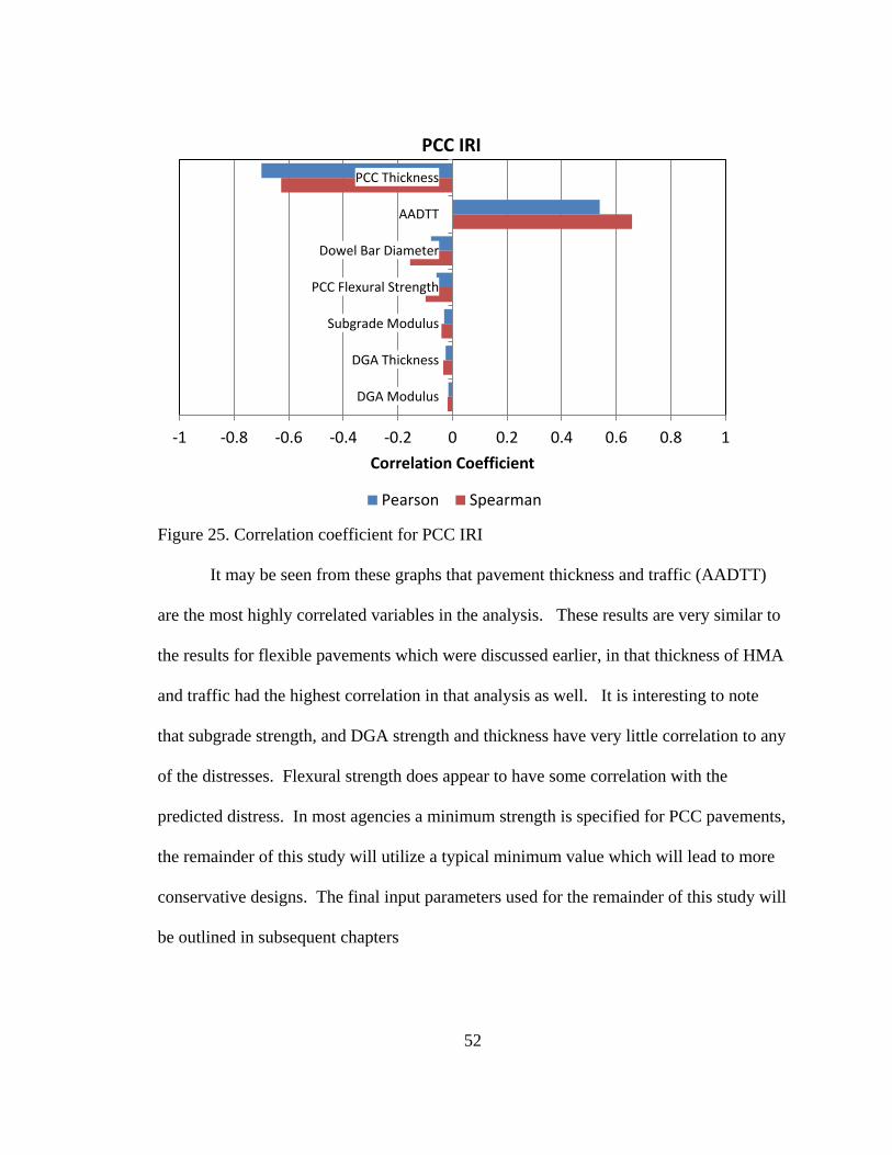
52
Figure 25. Correlation coefficient for PCC IRI It may be seen from these graphs that pavement thickness and traffic (AADTT)
are the most highly correlated variables in the analysis. These results are very similar to
the results for flexible pavements which were discussed earlier, in that thickness of HMA
and traffic had the highest correlation in that analysis as well. It is interesting to note
that subgrade strength, and DGA strength and thickness have very little correlation to any
of the distresses. Flexural strength does appear to have some correlation with the
predicted distress. In most agencies a minimum strength is specified for PCC pavements,
the remainder of this study will utilize a typical minimum value which will lead to more
conservative designs. The final input parameters used for the remainder of this study will
be outlined in subsequent chapters
-1 -0.8 -0.6 -0.4 -0.2 0 0.2 0.4 0.6 0.8 1
PCC Thickness
AADTT
Dowel Bar Diameter
PCC Flexural Strength
Subgrade Modulus
DGA Thickness
DGA Modulus
Correlation Coefficient
PCC IRI
Pearson Spearman

53
3.0 Design Reliability
3.1 Introduction
The Mechanistic-Empirical Pavement Design Guide (MEPDG) Version 1.1
developed under NCHRP 1-40 is a very complex tool for the evaluation of pavement
structures, with many input factors which characterize materials, climate, traffic and
construction. A key component of the design tool is the concept of design reliability.
The reliability is the probability that any particular type of distress (or combination of
distress manifestations) will remain below or within the permissible level during the
design life of the roadway (AASHTO, 1993). In the NCHRP MEPDG (NCHRP, 2004)
reliability is defined as the probability that each of the key distress types and smoothness
will be less than a selected critical level over the design period. In the previous
AASHTO 1993 Design Guide reliability was defined in terms of the number of
equivalent single axle loads to terminal serviceability being less that the number of
equivalent single axle loads actually applied (NCHRP, 2004).
The distresses predicted by the MEPDG represent mean values based on the
results of the design inputs being processed through the mechanistic model and then
applying transfer functions to determine predicted distresses. A reliability factor is then
applied to this mean value based on the accuracy of the prediction model. Therefore, the
basic results of the design guide are at a 50 percent reliability level, which means there is
a 50 percent chance that the predicted distress will be higher or lower than this value.
In the development of the NCHRP design guide, the original intent was to have a
full probabilistic analysis where designers would provide mean (average) input values for

54
various input parameters along with some measure of variability. These inputs were then
to be sampled using a Monte Carlo type of sampling to produce a true probabilistic
performance prediction. Due to the intensive computational time necessary to run a
single design (in excess of 20 minutes) this was not feasible.
3.2 MEPDG Reliability Concept
Several methodologies are available to conduct reliability based design, including
simulation methods (Monte Carlo Simulation) and other closed form analytical methods.
The reliability process in the new MEPDG is based on the ability of the performance
models to predict actual distresses of the sites used for calibration. The major
components of the errors associated with these predictions for rigid pavements were
defined by Darter (Darter, Khazanovich, Yu, & Mallela, 2005) as follows:
• Input Error -- error associated with the estimating each design input.
• Measurement Error of Distress – variation of measuring a given distress quantity.
• Pure Error – random or normal variability between distresses exhibited by exact replicate sections.
• Model or Fitting Error – inability of the model to predict actual pavement performance.
The reliability included in the new MEPDG was developed during the calibration
of the prediction models within the design guide. These prediction models consist of
“transfer functions” which predict a given distress based on measured pavement
responses. These transfer functions were calibrated utilizing data from national Long
Term Pavement Performance (LTPP) and another field pavement studies across the
country. The LTPP project was a national study on which contained over 800 pavement

55
sections across the country (Stubstad, Tayabji, & Lukanen, 2002). These pavement
sections were periodically reviewed for performance. In addition, extensive testing was
conducted to determine the various engineering properties of the pavement structure.
The general concept for reliability uses the standard deviation of the prediction
model (standard error of the estimate) to determine the appropriate design reliability.
An example of the process utilized to determine this reliability is given below.
Figure 26 provides an example plot of the predicted versus measured slab cracking for
jointed plane concrete pavements, the results are broken up into four regions. These
regions will be used to segment the variability in the predicted performance.
Figure 26. Example of accuracy of MEPDG prediction model (Darter M. , 2007)

56
It may be seen from the scatter in the data in Figure 27 that the difference between
the measured and predicted data is quite significant in many areas. These residuals
(measured – predicted distress) are used to determine the variability of the prediction
model at various levels of distress.
The distress data utilized for calibration were then analyzed further by
determining the mean and standard deviation of the predicted and measured data within
each group (NCHRP, 2003). It was assumed that the data within each group is normally
distributed and therefore techniques relating to standard normal distributions may be
used. Relationships were then developed to relate the grouped information for the
measured and predicted distress
In Figure 26, four areas are identified at various measured distress levels. Within
each of these areas, the standard deviation of the residual is determined and utilized as the
measure of model variability within that ranges. These discrete values are then used to
develop a relationship relating the standard deviation versus predicted distress for the full
range of anticipated results. An example of this method is given in Figure 27 below.

57
Figure 27. Variable standard deviation used for reliability analysis (Darter M. , 2007)
The final step to evaluate the reliability utilized in the MEPDG involved relating
the predicted distress to the standard deviation of the measured distress for each group.
This standard deviation may then be used to calculate the reliability of the predicted
distress at any level.
This standard deviation relationship or residual error contains all the available
information regarding the ways in which the prediction model fails to properly explain
the observed distress (scatter in predicted results). The relationship in Figure 27 is
defined as follows:
Predicted PCC Pavement Cracking

58
𝑆𝑇𝐷𝑐 = −0.00172 ∗ 𝐶𝑅𝐴𝐶𝐾502 + 0.3447 ∗ 𝐶𝑅𝐴𝐶𝐾50 + 4.6772
where:
STDC = standard deviation for cracking
CRACK50 = predicted cracking (50% reliability)
The resulting standard deviation and the cracking at 50% reliability may be used to
determine the cracking at any given reliability level based on the assumption that these
standard deviations are normally distributed. This method is illustrated as follows:
𝐶𝑅𝐴𝐶𝐾𝑅 = 𝐶𝑅𝐴𝐶𝐾50 + 𝑆𝑇𝐷𝐶 ⋅ 𝑍𝑅
where:
CRACKR = predicted cracking at reliability level R, percent slabs
CRACK50 = predicted cracking based on mean inputs (50% reliability), percent slabs STDC = standard deviation of cracking at predicted level of mean cracking ZR = standard normal deviate (one-tailed)
This concept is graphically illustrated in Figure 28.
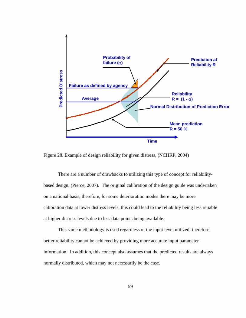
59
Figure 28. Example of design reliability for given distress, (NCHRP, 2004)
There are a number of drawbacks to utilizing this type of concept for reliability-
based design. (Pierce, 2007). The original calibration of the design guide was undertaken
on a national basis, therefore, for some deterioration modes there may be more
calibration data at lower distress levels, this could lead to the reliability being less reliable
at higher distress levels due to less data points being available.
This same methodology is used regardless of the input level utilized; therefore,
better reliability cannot be achieved by providing more accurate input parameter
information. In addition, this concept also assumes that the predicted results are always
normally distributed, which may not necessarily be the case.
Probability offailure (α)
Mean predictionR = 50 %
ReliabilityR = (1 - α)
Prediction atReliability R
Average
Failure as defined by agency
Time
Pred
icte
d D
istr
ess
Normal Distribution of Prediction Error

60
A study has been undertaken to evaluate the impact of input parameter
distributions on the predicted performance and its reliability (Graves & Mahboub, 2011).
This study outlines a potential means to utilize simulation-based techniques (Monte
Carlo) to evaluate the variation in predicted performance based on the variability of a set
of input parameters for a specific pavement design section. Other work has illustrated the
use of simulation techniques to conduct sensitivity analysis for the MEPDG Design
Guide (Graves & Mahboub, 2006). This study will utilize similar techniques, but will
include input distributions which represent the anticipated variability for a given
pavement design project.
3.3 Input Parameter Variability
Many factors are involved in establishing the appropriate input variability for a pavement
design. Considerable work has been done in recent years evaluating the variability of
pavement construction parameter (NCHRP Project 20-50), (Stubstad, Tayabji, &
Lukanen, 2002). The results of this work provide insight into the variability of in-situ
pavement materials, both their strength and the thickness at which they were constructed.
This information provides a measure of the potential variability which may occur in the
construction of roadways. A brief summary of coefficients of variation from
backcalculated layer moduli for selected pavement materials obtained from this study are
given in Table 13.

61
Table 13. Coefficient of Variation of Backcalculated Moduli
Layer
CV’s Recommended for Pavement Design
Average (%) Lower (%) Upper (%) Asphalt Concrete 39 17 72 Granular Base 50 17 92 Granular Subbase 74 16 150
Subgrade 35 6 92
Table 13 illustrates that all of the coefficients of variation for each design
parameter are greater than 30%. For layer thicknesses, the NCHRP research indicated
that for unbound layers the 85th percentile thickness variation would be 0.5 inches and 0.3
inches for asphalt bound layers.
For the evaluation of the reliability of the MEPDG process, data from the NCHRP
project discussed above along with data obtained from quality control information from
the Kentucky Transportation Cabinet was utilized. The data from the Kentucky
Transportation Cabinet included both historical material quality control reports within
Kentucky and their current quality control standards (KYTC, 2008). Based on these
sources of data, reasonable variation of selected input parameters was determined.
Since the goal of this study was to evaluate the variability of a specific design, in
addition to these asphalt volumetric parameters, information regarding the aggregate
structure of the mix is also necessary. A single gradation for the surface was utilized,
while two gradations for the HMA base were used. This decision was made based on
review of several QC/QA reports for Kentucky projects, which indicated that the

62
variation on gradation for the surface was very small, while greater variation in the base
layer gradation was observed.
Aggregate specific gravities were selected for a given aggregate source typical for
Kentucky. It was assumed that this would remain constant for a specific construction
project. Therefore, it was assumed, that constant values of maximum specific gravity
(Gmm) and bulk specific gravity of the aggregate (Gsb) could be utilized. Based on these
assumptions, in conjunction with the parameters listed in Table 13, the bulk specific
gravity of the mix (Gmb) and resulting unit weight at various void contents may be
determined. In addition, once the Gmb is known, the mixture VMA may then be
calculated for each Gmb and asphalt content. Once the VMA is known, it may be used in
conjunction with air voids to determine the effective binder content (by volume) used in
Level 3 of the MEPDG software. These properties are linked together to provide realistic
information regarding the mix instead of just varying each parameter across a range
independently
In addition to the HMA mix parameters, variability in Average Annual Daily
Truck Traffic (AADTT), dense-graded-aggregate (DGA) base (thickness and strength),
HMA base thickness, and subgrade strength were included. The discrete values used for
the normal distribution for each is given in Table 14.
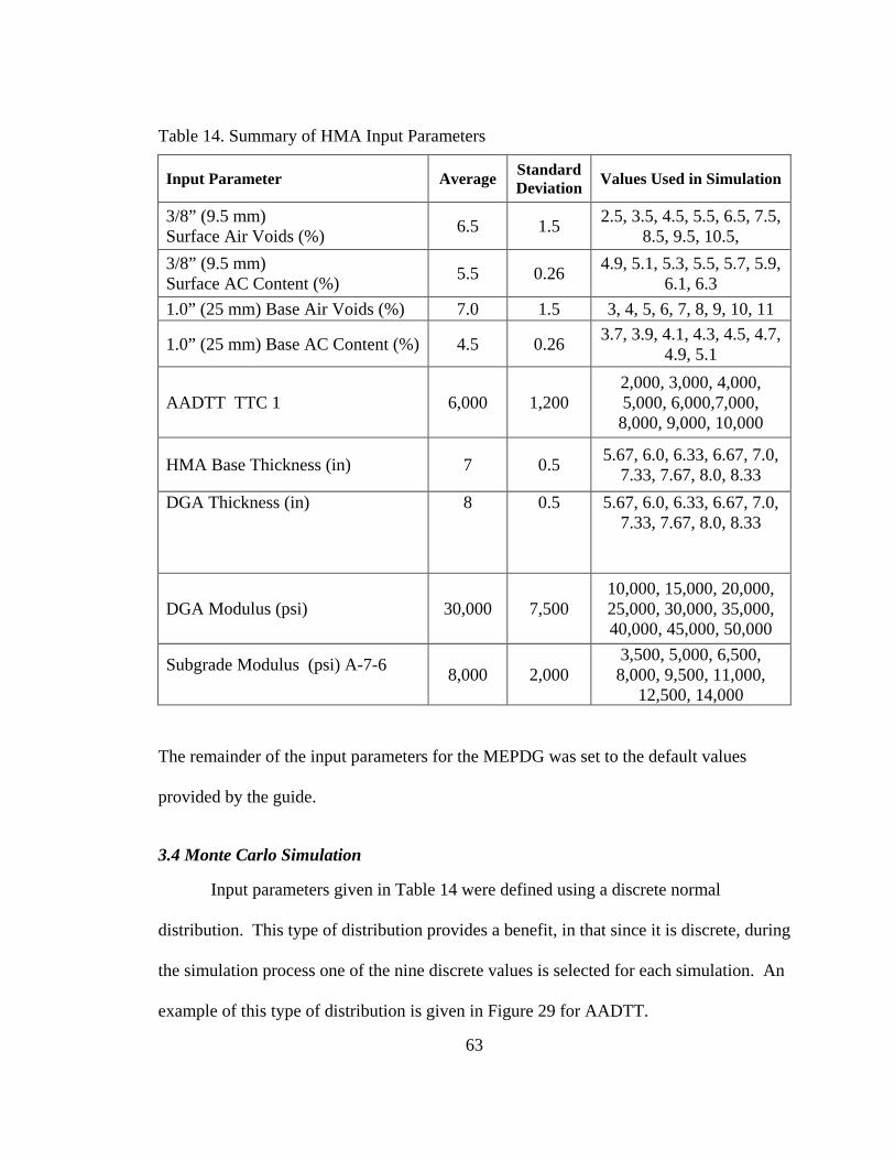
63
Table 14. Summary of HMA Input Parameters
Input Parameter Average Standard Deviation Values Used in Simulation
3/8” (9.5 mm) Surface Air Voids (%) 6.5 1.5 2.5, 3.5, 4.5, 5.5, 6.5, 7.5,
8.5, 9.5, 10.5, 3/8” (9.5 mm) Surface AC Content (%) 5.5 0.26 4.9, 5.1, 5.3, 5.5, 5.7, 5.9,
6.1, 6.3 1.0” (25 mm) Base Air Voids (%) 7.0 1.5 3, 4, 5, 6, 7, 8, 9, 10, 11
1.0” (25 mm) Base AC Content (%) 4.5 0.26 3.7, 3.9, 4.1, 4.3, 4.5, 4.7, 4.9, 5.1
AADTT TTC 1 6,000 1,200 2,000, 3,000, 4,000, 5,000, 6,000,7,000, 8,000, 9,000, 10,000
HMA Base Thickness (in) 7 0.5 5.67, 6.0, 6.33, 6.67, 7.0, 7.33, 7.67, 8.0, 8.33
DGA Thickness (in)
8
0.5
5.67, 6.0, 6.33, 6.67, 7.0, 7.33, 7.67, 8.0, 8.33
DGA Modulus (psi) 30,000 7,500 10,000, 15,000, 20,000, 25,000, 30,000, 35,000, 40,000, 45,000, 50,000
Subgrade Modulus (psi) A-7-6 8,000 2,000
3,500, 5,000, 6,500, 8,000, 9,500, 11,000,
12,500, 14,000
The remainder of the input parameters for the MEPDG was set to the default values
provided by the guide.
3.4 Monte Carlo Simulation
Input parameters given in Table 14 were defined using a discrete normal
distribution. This type of distribution provides a benefit, in that since it is discrete, during
the simulation process one of the nine discrete values is selected for each simulation. An
example of this type of distribution is given in Figure 29 for AADTT.

64
Figure 29. Example discrete normal distribution
With a typical normal distribution, during simulation the number of values which
could be selected is theoretically infinite. The use of the discrete normal distribution
provides a means to sample the entire space of a given variable with fewer simulations.
These discrete distributions were then sampled using a Monte Carlo random sampling
routine (Helton, 2004), to produce 100 different design scenarios covering the complete
range of the input parameter space. The remaining variables necessary to evaluate the
design were assigned default values based on the MEPDG software. These 100 scenarios
were then processed through the MEPDG software to produce a matrix of outputs for the
following distresses: fatigue cracking, HMA rutting, total rutting, transverse cracking
0
0.05
0.1
0.15
0.2
0.25
0.3
0.35
0 2000 4000 6000 8000 10000 12000
Prob
abili
ty
AADTT

65
and IRI. For this particular design section, less than 5 percent of the scenarios showed
any longitudinal cracking or transverse cracking. Therefore, these distresses were not
included in the remainder of the analysis.
3.5 Evaluation of Distress Prediction Reliability
To evaluate the variability of the predicted distresses, a cumulative distribution
was calculated for each predicted distress at the 10-year level. From these distributions
the reliability at a given distress level may be determined. Cumulative distributions are
illustrated in Figure 30 through Figure 32. In each figure, the 90th percent reliability is
also noted. Some are nearly normally distributed, while others appear to be skewed.
Figure 30. Cumulative distribution of fatigue cracking

66
Figure 31. Cumulative distribution of total rutting
Figure 32. Cumulative distribution of IRI

67
There are a variety of methods to evaluate the normality of a given distribution.
One such graphical method is presented in Figure 33 through Figure 35. This method
involves plotting the cumulative distribution of a given distress against the standard
normal quantiles of a normal distribution (Park, 2012). This quantile – quantile (Q-Q) is
a plot of the percentiles (or quintiles) of a standard normal distribution versus the
corresponding percentiles of the observed data. If the observations follow approximately
a normal distribution, the resulting plot should be roughly a straight line with a positive
slope.
Figure 33. Normal quantiles, fatigue cracking
Mean 4.55 Standard Deviation 4.77 Skewness 2.26 Kurtosis 5.46

68
Figure 34. Normal quantiles, total rutting
Figure 35. Normal Quantiles, IRI
Mean 0.79 Standard Deviation 0.11 Skewness 0.79 Kurtosis 0.54
Mean 109.34 Standard Deviation 6.37 Skewness 1.05 Kurtosis 0.91

69
In Figure 33 through Figure 35 the dashed line is a reference for what the data
should look like if it were normally distributed. It may be seen that from these figures
that fatigue cracking is somewhat skewed to the lower cracking values, while total
rutting along with IRI are more near the reference line, but still indicate that they may not
be normally distributed.
To further evaluate the normality of the predicted tests, the Skewness and
Kurtosis for each predicted distress were determined. Skewness and Kurtosis are terms
that describe the shape and symmetry of the distributions.
Skewness is a measure of symmetry, or lack thereof. A value greater than 1 or
less than -1 indicates a highly skewed distribution, between 0.5 and 1.0 or -0.5 and -1.0 is
moderately skewed, and between -0.5 and 0.5 indicates a fairly symmetric distribution, or
nearly normally distributed. Positive skewness indicate distributions are skewed to the
left, or lower values, while negative skewness are skewed to the right indicating higher
values.
Kurtosis is a measure of the heaviness of the tails of a distribution. A normal
distribution has its kurtosis equal to zero. Extremely non-normal distributions may have
high positive or negative kurtosis values, while nearly normal distributions will have
kurtosis values close to zero. Kurtosis is positive if the tails are "heavier" than for a
normal distribution and negative if the tails are "lighter" than for a normal distribution
(SAS, 2006).
The Skewness and Kurtosis for each predicted distress are given in Figure 33
through Figure 35. In review of these statistics, it may be seen that all the distress types

70
have Skewness that is greater than 0.5, indicating that the data are skewed toward lower
levels. Two of the distresses, IRI and fatigue cracking have Skewness greater than 1.0
indicating that they are significantly skewed toward lower values. All of the distributions
except AC rutting have high positive Kurtosis, which would indicate the tails of the
distribution are heavier than a normal distribution. The Kurtosis for AC rutting is nearly
zero, indicating that it is approaching the symmetry of a normal distribution.
Another method to test for normality is to perform a Shapiro-Wilk test (Park,
2012). This test examines the null hypothesis that a particular sample came from a
normally distributed population. For each of the distributions given in Figure 33 through
Figure 35, the null hypothesis that the data are normally distributed is rejected.
These results are interesting in that each of the input levels were normally
distributed, but the predicted distresses do not appear to be normally distributed. This is
not entirely unexpected since the MEPDG is a very complex model, which has many
interactions between input variables which may or may not be linear. However, the
reliability in the current MEPDG is based on assumptions that the residual error
associated with mean inputs compared to actual measured distress is normally distributed.
A comparison of 90 percent reliability given by the MEPDG for mean inputs of the
variables in this study and the reliability given from the simulation results may be seen in
Table 15.
Table 15. Comparison of 90 percent Reliability from MEPDG and Simulation Model
Distress MEPDG Simulation Fatigue Cracking (%) 15.4 10.8 Total Rutting (in) 0.970 0.934 IRI (in/mi) 147.4 117.2

71
Some of the distresses have significant differences between the MEPDG and
Simulation reliability at the 90 percent level. For fatigue cracking, the MEPDG value
was 50% higher than that of the simulation results, while rutting and IRI were somewhat
closer together. This may be explained to some extent by the fact that the prediction
models for rutting and IRI generally have less model error as indicated by higher R2 and
lower standard errors than do fatigue cracking models, as described in the recently
released NCHRP Research Results Digest (NCHRP, 2006). A full understanding of this
difference is necessary, so that designers can have the best possible confidence in the
predictions provided by the MEPDG software. Additionally, the observed departure
from normality of various distress modes may impact the reliability of the design. High-
type pavements are designed to perform without distresses exceeding a low threshold. It
is indeed at these low thresholds levels where significant departures from normality take
place under the current models. Therefore, any reliability-based analysis for high-type
pavement facilities would seem suspect at this time. A similar argument can be made for
the low-volume roads, in which distress thresholds are much higher. Only the mid-
ranges of the distress modes seem to follow normal distributions.
As was discussed earlier, the reliability in the MEPDG is assumed to be all
inclusive and account for all errors, such as: input error, distress measurement error, pure
error, and model fitting error. It may be seen from these results that the 90 percent
reliability based on simulation of the variation in input parameters is less in all cases than
that predicted by the MEPDG. This would indicate that some of the other errors in the

72
prediction model (measurement error, pure error or model fitting error) have some
significant impact on the MEPDG reliability.
These results may also indicate that continued refinement of the reliability portion
of the MEPDG may be useful. It is not apparent at the time of preparation of this report
what changes may have been made to the reliability calculations during the recalibration
of distress models included in Version 1.1 of the MEPDG software. Data were not
readily available in the literature regarding the distributions of the residuals for the
measured versus predicted distresses for the new models. Therefore, continued work in
this area is recommended.
This analysis provides a means to quantify the variability of the MEPDG distress
predictions based on the variation in typical design inputs. It would indicate that for
some of the distresses (fatigue cracking, and IRI) the variability not associated with input
variability may be quite significant.
3.5 Summary of Results
This study has illustrated that the variability of the MEPDG predicted output for a
given design section may not be normally distributed across typical variations of project
input parameters. This was evident from the use of quantile plots to evaluate the shape of
the predicted distributions. In addition, Skewness and Kurtoses statistics indicate that the
predicted distresses were not normally distributed. The Shapiro-Wilk test also indicated
the distributions were not normal. Since the current MEPDG reliability relies on
assumption of normality for the performance prediction errors or residuals to determine
reliability, further work may be necessary to develop alternative methods to address

73
reliability. One method may be to follow the same process which is currently utilized,
but instead of making the assumption of normality, actual distributions of error/residuals
could be used.
The departure from normality of various distress modes has the potential to
impact the reliability of designs. Since high-type pavements are designed with very low
distress thresholds, where the departures from normality take place under the current
models, designs of this type of projects could be suspect. The same argument could also
be made for lower volume facilities, which are designed for high distress levels which
also exhibit departure from normal distributions. Further understanding of this variability
is necessary to insure pavement designers can effectively utilize the correct reliability in
design, and achieve the pavement performance they are expecting.
As computational efficiency and streamlining of the MEPDG software continues,
the use of additional simulation techniques will become more feasible. Similar
methodologies (Darter, Khazanovich, Yu, & Mallela, 2005) have been suggested in the
literature, but have not been implemented due to the computationally intensive analysis
required.
This study has outlined the potential contribution of material input variability to
the overall reliability predicted by the design guide. As computational efficiency
continues to increase, this type of process could be utilized to further investigate the
reliability portion of the design guide.

74
4.0 Streamlined Model Development
4.1 Introduction
The Mechanistic Empirical Pavement Design Guide (MEPDG) (NCHRP, 2004),
developed by the National Cooperative Highway Research Program (NCHRP) is a very
robust and powerful tool for the analysis and design of highway pavements. The
software does require some trial and error processing to determine the optimal design
based on selected required performance. The user will select a trial design, allow the
software to predict performance and then adjust design parameters if the required
performance is not met.
The ability to streamline this process and reduce the potential number of required
interactions would improve the use of the design guide on routine designs. The
streamlining process outlined in this project will provide a means to determine a better
starting point for determining the optimal design. It will provide the designer with an
estimate of the required design thicknesses which can then be run through the full
MEPDG model for performance final prediction.
The recently released DARWin-ME (AASHTO, 2011) software does include an
optimization routine which automates the process of evaluating different structural
thicknesses around a base design. However, it still requires multiple runs of the
DARWin-ME software. The procedure is still an analysis procedure which does not
allow for a direct solution for pavement thickness. The most recent version of the
software still requires more than fifteen minutes of runtime, for a single flexible

75
pavement analysis. Rigid pavement projects run somewhat faster, but still require at least
five minutes to complete a single analysis. Both of these runtimes are achieved using a
very high end, six-core personnel computer with 12 MB of RAM. For an average user
the process can still be quite cumbersome and time consuming.
The factors mentioned above illustrate the need to develop some type of
streamlined procedure to utilize this new methodology. The development of a
streamlined process will allow designers to more effectively utilize the tools they have at
their disposal, by optimizing the amount of time needed to conduct pavement designs.
4.2 Selection of Modeling Methodology
As has been discussed the MEPDG model is a very complex procedure, in
addition, all of the underlying analysis algorithms and source code are not available.
Therefore, a direct evaluation of all the models and streamlining their use is not a viable
alternative. The lack of access to all of these models also forces the streamlining to take
place using some form of nonparametric model. Nonparametric models are developed
with no understanding of the underlying model form or the interactions between
variables. All of this information is derived from the actual data set being modeled.
In working to streamline the MEPDG several methodologies were investigated as
potential means to develop the streamline model, one was the use of Neural Networks
another was Multiple Adaptive Regression Splines (MARS). Many comparative studies
have been conducted (Francis, 2003; Cogger, 2001; Abraham & Steinberg, 2004; De
Veauz, Pischogios, & Ungar, 1993), these studies have identified some of the strengths

76
and weaknesses of each method. Neural Networks are very powerful tools in looking at
complex problems; one of their drawbacks has been that they are generally “Black Box”
analysis procedures, in that their results are generally very complex and not easily
understood and can be difficult to implement into practical solutions.
The MARS technique (Friedman, 1991) is a multivariate, nonparametric
regression technique which has been used in a variety of applications in many disciplines.
It does not require any assumptions about the relation between dependent and
independent variables and develops the relationship between those variables in a
piecewise regression function.
Nonparametric regression techniques not only relax the assumption of linearity
and normality of relationships, they do not require the functional relationship between the
response and repressor variables to be known. Nonparametric models typically grow in
size to accommodate the complexity of the data. This is a form of regression analysis in
which the predictor does not take a predetermined form but is constructed according to
information derived from the data. This method only connects the input variables to the
output results. In the case of the MARS models developed during the research, no
information is necessary regarding the transfer functions which are included in the
MEPDG software, the MARS models developed are completely independent of what
may be occurring within the “black box” of the MEPDG software. Nonparametric
regression is a form of regression analysis in which the predictor does not take a
predetermined form but is constructed according to information derived from the data.

77
Nonparametric regression requires larger sample sizes than regression based on
parametric models because the data must supply the model structure as well as the model
estimates.
This method has the ability to easily analyze complex situations and include both
nonlinear relationships and interactions among variables. One key advantage to the
MARS method is the ability to take the model results and implement them into a variety
of applications. The basis functions in the MARS model provide information on the
breakpoints or changes in the input parameter space which impact the model result.
4.3 Overview of Multiple Adaptive Regression Splines Model
The MARS methodology was introduced by Stanford physicist and statistician
Jerome Friedman (Friedman, 1991). MARS is an innovative modeling tool that provides
an excellent tool in finding optimal variable transformations and interactions.
There are three main steps to fit a MARS model. First is the construction phase,
where basis functions (BF) are introduced in several regions of the predictors
(independent variables). These basis functions are then combined into a weighted sum to
define the global MARS model. These basis functions generally define where the piece-
wise regression model changes or “hinges”. This model normally contains many basis
functions, which can cause over-fitting of the model. The second step is to prune the
basis functions that have caused the over-fitting. The third and final step is to select the
optimal model from the remaining smaller models which have resulted from the pruning.
A more detailed discussion of the MARS technique is outlined by Friedmen (Friedman,
1991).

78
The procedure is a form of nonparametric regression, therefore making no
assumptions about the underlying functional relationship between the dependent and
independent variables. Some have described the process as the “Divide and Conquer”
strategy where the input space is divided into regions each with its own regression
equation. It provides a means to develop flexible regression models by fitting separate
splines (or basis functions) to intervals of the predictor variables. The variables used and
the end points of the intervals for each variable, referred to as knots are found via a brute
force mathematical routine. Variables, knots and interactions are optimized
simultaneously by evaluating a "loss of fit" (LOF) criterion. MARS chooses the LOF that
most improves the model at each step. In addition to searching variables one by one, it
also searches for interactions between variables, allowing any degree of interaction to be
considered.
The output from the MARS procedure is a model that can be easily understood.
Others have concluded that MARS has specific advantages over more complicated
techniques such as neural networks, in that it has the ability to be easily implemented into
other applications.

79
The general model of the MARS technique may be represented by the following
equations. MARS can be viewed as a generalization of stepwise linear regression
method. Which uses expansions in piecewise linear basis functions of the form (Haleem,
Abdel-Aty, & Santos, 2010):
(x − t)+ and (t − x)+. The “+” means positive part, so
(𝒙 − 𝒕)+ = �𝒙 − 𝒕, 𝒊𝒇 𝒙 > 𝒕𝟎, 𝒐𝒕𝒉𝒆𝒓𝒘𝒊𝒔𝒆 𝒂𝒏𝒅 (𝒕 − 𝒙)+ = �𝒕 − 𝒙, 𝒊𝒇 𝒙 < 𝒕
𝟎, 𝒐𝒕𝒉𝒆𝒓𝒘𝒊𝒔𝒆
A graphical representation of this is given in Figure 36.
Figure 36. Basis function used by MARS (Hastie, Tibshirani, & Friedman, 2001)
In the example the location where t = 5,000 is called the knot with a pair of
splines intersecting at this location. The model-building follows a pattern like a forward

80
stepwise linear regression, with the exception that instead of using the original input
values, we us functions which are developed using the Basis Functions created from the
input values. The general form of the model is as follows:
𝒚� = 𝒂𝟎 + � 𝒂𝒎 𝑩𝒎
𝑴
𝒎=𝟏
(𝒙)
Where:
ŷ is the predicted response:
a0 is the coefficient of the constant basis function:
Bm(x) is the mth basis function, which can be a single spline function or an interaction of two (or more) spline functions;
am is the coefficient of the mth basis function; and
M is the number of basis functions included in the MARS model
Generalized cross-validation (GVC) is used to evaluate the quality of the fit of the
models. This procedure is used to determine which variables to keep within the model,
therefore, producing the best fit. The GVC is also used to rank the variables in terms of
importance; the GVC is computed with and without each variable in the model to
determine their importance. The general form of the GVC is as follows:

81
𝐺𝑉𝐶 = 1𝑁��
𝑦𝑖 − 𝑓(𝑥𝑖)
1 − 𝑘𝑁
�
2
𝑁
𝑖=1
Where:
N is the number of observations
y is the dependent variable
x is the independent variable(s)
k is the effective number of parameters or degrees of freedom in the model
The MARS process was implemented using the MARS 2.0 (Salford Systems,
2009) software developed by Salford Systems. This software provides an interactive
interface to the MARS algorithms which facilitate the model development. The models
developed by the MARS procedure can be easily programed in a variety of languages
including C, visual basic for applications (VBA). Visual Basic has been utilized for this
research to facilitate the use of the MARS models developed. . An example of a typical
MARS model is given in the following equation:
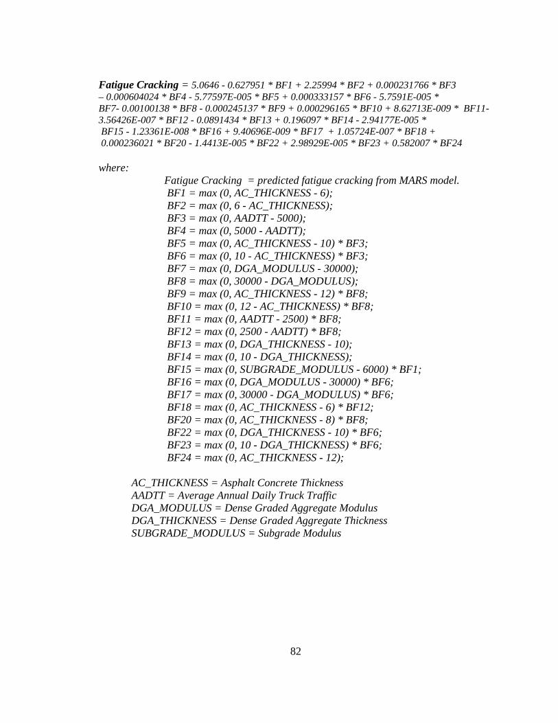
82
Fatigue Cracking = 5.0646 - 0.627951 * BF1 + 2.25994 * BF2 + 0.000231766 * BF3 – 0.000604024 * BF4 - 5.77597E-005 * BF5 + 0.000333157 * BF6 - 5.7591E-005 * BF7- 0.00100138 * BF8 - 0.000245137 * BF9 + 0.000296165 * BF10 + 8.62713E-009 * BF11- 3.56426E-007 * BF12 - 0.0891434 * BF13 + 0.196097 * BF14 - 2.94177E-005 * BF15 - 1.23361E-008 * BF16 + 9.40696E-009 * BF17 + 1.05724E-007 * BF18 + 0.000236021 * BF20 - 1.4413E-005 * BF22 + 2.98929E-005 * BF23 + 0.582007 * BF24 where:
Fatigue Cracking = predicted fatigue cracking from MARS model. BF1 = max (0, AC_THICKNESS - 6); BF2 = max (0, 6 - AC_THICKNESS); BF3 = max (0, AADTT - 5000); BF4 = max (0, 5000 - AADTT); BF5 = max (0, AC_THICKNESS - 10) * BF3; BF6 = max (0, 10 - AC_THICKNESS) * BF3; BF7 = max (0, DGA_MODULUS - 30000); BF8 = max (0, 30000 - DGA_MODULUS); BF9 = max (0, AC_THICKNESS - 12) * BF8; BF10 = max (0, 12 - AC_THICKNESS) * BF8; BF11 = max (0, AADTT - 2500) * BF8; BF12 = max (0, 2500 - AADTT) * BF8; BF13 = max (0, DGA_THICKNESS - 10); BF14 = max (0, 10 - DGA_THICKNESS); BF15 = max (0, SUBGRADE_MODULUS - 6000) * BF1; BF16 = max (0, DGA_MODULUS - 30000) * BF6; BF17 = max (0, 30000 - DGA_MODULUS) * BF6; BF18 = max (0, AC_THICKNESS - 6) * BF12; BF20 = max (0, AC_THICKNESS - 8) * BF8; BF22 = max (0, DGA_THICKNESS - 10) * BF6; BF23 = max (0, 10 - DGA_THICKNESS) * BF6; BF24 = max (0, AC_THICKNESS - 12);
AC_THICKNESS = Asphalt Concrete Thickness AADTT = Average Annual Daily Truck Traffic DGA_MODULUS = Dense Graded Aggregate Modulus DGA_THICKNESS = Dense Graded Aggregate Thickness SUBGRADE_MODULUS = Subgrade Modulus

83
4.4 Overview of Datasets used for Modeling
The datasets used for the development of the streamlined model are based on the
MEPDG program that was developed during the NCHRP 1-37A project. These data sets
consist of multiple analysis runs over a range of values for selected design inputs. The
selection of these variables was based on the sensitivity analysis outlined in the previous
chapter and experience working with Kentucky’s mechanistic-empirical pavement design
procedure. Streamlined models have been developed for both flexible pavements (HMA
pavements) and rigid pavements (PCC pavements).
A summary of the variables utilized in each of these designs is given in Table 16.
For the development of these models all required input values for climate, bound and
unbound materials, and traffic which are not included in Table 16, were held constant,
information regarding these default values may be found in previous research by the
authors (Graves & Mahboub, 2006).
Table 16. Summary of Variables in the Streamlined Model
Flexible Pavement Rigid Pavements AADTT AADTT
HMA Thickness PCC Thickness DGA Thickness DGA Thickness DGA Modulus DGA Modulus
Subgrade Modulus Dowell Bar Diameter
To develop the streamlined models, a series of designs were developed and
processed through the NCHRP design software, these designs were randomly selected
from the input parameter set of possible design combinations. Table 17and Table 18

84
provide a summary of the input variable combinations possible for each type of
pavement. The AADT levels indicated were the current year AADTT and this traffic
level was projected for 20-years at two percent growth per year. Therefore, the distresses
predicted are those which occur at the end of a 20-year design life.
A full factorial matrix of the input parameters would require several thousand
different design runs to be completed. Each of these design runs takes in excess of 30
minutes to complete. There are multiple methods which could be utilized to minimize
the number of design runs to be completed. One such method would be to conduct a
fractional factorial design, which would reduce the number of required MEPDG design
runs by the selected fraction ½, ¼, etc. Once the fractional number was selected, some
type of methodology would be necessary to insure the entire input parameter space is
included. A second method, which was used in this analysis was a random sampling
technique using discrete uniform distributions, which would allow for equal probability
in sampling across the entire input parameter space. The final result was a set of 1,500
different pavement designs for each of the pavement types, these designs were utilized to
develop the streamlined models. With this large dataset of solutions, one could simply
utilize some type of search routine to determine the design which most closely fits the
required performance parameters for design. However, this may not provide the most
efficient design since the thickness increments are at least one inch apart.

85
Table 17. Flexible Pavement Input Variables
AADTT (Average Annual Daily Truck Traffic)
500, 2,500, 5,000, 7,500, 10,000, 15,000, 20,000, 25,000
HMA Thickness (in) 4, 6, 8, 10, 12, 14
DGA Thickness (in) 6, 8, 10, 12, 14, 16
DGA Modulus (psi) 20,000, 25,000, 30,000, 35,000, 40,000
Subgrade Modulus (psi) 6,000, 7,500, 9,000, 10,500, 12,000, 13,500
Table 18. Rigid Pavement Input Variables
AADTT (Average Annual Daily Truck Traffic)
500, 2,500, 5,000, 7,500, 10,000, 15,000, 20,000, 25,000
PCC Thickness (in) 6, 8, 10, 12, 14
DGA Thickness (in) 6, 8, 10, 12, 14, 16
DGA Modulus (psi) 20,000, 25,000, 30,000, 35,000, 40,000
Subgrade Modulus (psi) 6,000, 7,500, 9,000, 10,500, 12,000, 13,500
Dowel Bar Diameter (in) 1.25, 1.5, 1.70
The streamlined model provides a means to go from a discrete set of solutions to a
continuous solution space which will allow the designer to determine the most efficient
design.
The development of these design scenarios is a very time consuming process.
Two Master’s Degree students (Ganapathy Palanisamy and Salman Hakimzadeh) assisted
in the operation of the design software to process the design scenarios selected. Each
design scenario must be entered into the design software and processed. Once all of the
designs had been processed, the resulting predicted performance (output files) must be

86
combined into a database which provides a listing of the input parameters and the output
parameters for each design evaluated.
To facilitate the input of the information into the design software, an automation
program, Automation Anywhere 4.0 (Automation Anywhere, 2006) was utilized. This
program read information from the spreadsheet of desired input values and input it into
the interactive design software.
These input files were then processed through a batch process available in the software.
The resulting predicted distresses are stored in an Excel spreadsheet for use by the
designer. An Excel macro was developed to extract data from each of these spreadsheets
and combine it with the database of input solutions. The advantage of utilizing this type
of process was that the potential of user input error was reduced, and the speed of
developing the input files was increased. Once completed, this database provided the
necessary data used to develop the streamlined models.

87
4.5 Development Model for Flexible Pavements
The database of design scenarios which was previously discussed was used as the
input information for the streamlined MARS models. Two different sets of models have
been developed. The first set of models was developed to predict individual distresses of
rutting, fatigue cracking, and roughness (IRI). The general form of the models which
were developed are given below, the actual models for each is given in Appendix A:
Fatigue Cracking (%) = f (AC thickness, DGA thickness, subgrade modulus, DGA modulus, and AADTT)
Rutting (in) = f (AC thickness, DGA thickness, subgrade modulus, DGA modulus, and AADTT)
Roughness, IRI (in/mi) = f (AC thickness, DGA thickness, subgrade modulus, DGA modulus, and AADTT)
where: Fatigue Cracking (%) = predicted flexible pavement fatigue cracking Rutting (in) = predicted flexible pavement rutting Roughness (in/mi) = predicted flexible pavement roughness AC Thickness (in) = thickness of asphalt bound surface layer DGA Thickness (in) = thickness of unbound dense graded aggregate Subgrade modulus (psi) = subgrade strength in terms of resilient modulus
DGA modulus (psi) = unbound dense graded aggregate base in terms of resilient modulus AADTT = average annual daily truck traffic
These models will predict pavement performance based on the input parameters
similar to the results of the full MEPDG software. They can be utilized as a pavement
analysis tool by predicting anticipated pavement performance. MARS models were
developed for each of the above listed relationships; the resulting R2 for each of these
models was in excess of 0.9. Once the models were developed they were used to

88
compute the specified distress and then compared to the actual distress in the input
database as determined by the MEPDG model. These results are given graphically in
Figure 37 through Figure 39. It may be seen from each comparison that the predicted
distress from the MARS model and the actual distress from the MEPDG model correlate
very well.
Figure 37. Comparison of actual IRI and MARS predicted IRI
100
110
120
130
140
150
160
170
180
190
200
210
220
100 110 120 130 140 150 160 170 180 190 200 210 220
Pred
icte
d M
ARS
IRI (
in/m
i)
Actual IRI (in/mi))

89
Figure 38. Comparison of total rutting with MARS predicted total rutting
Figure 39. Comparison of fatigue cracking with MARS predicted fatigue cracking
0
0.2
0.4
0.6
0.8
1
1.2
1.4
1.6
0 0.2 0.4 0.6 0.8 1 1.2 1.4 1.6
Pred
icte
d M
ARS
Rutt
ing
(in)
Actual Rutting (in)
0
10
20
30
40
50
60
70
0 10 20 30 40 50 60 70
Pred
icte
d M
ARS
Fatig
ue C
rack
ing
g(%
)
Actual Fatigue Cracking (%)
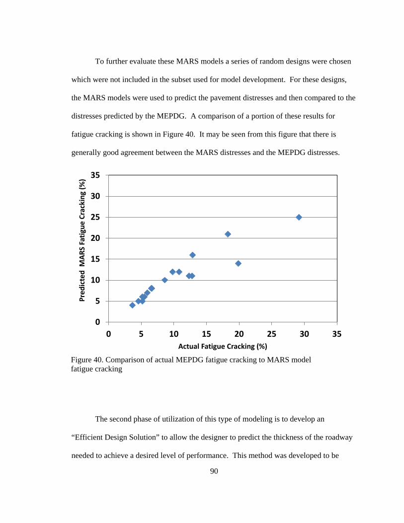
90
To further evaluate these MARS models a series of random designs were chosen
which were not included in the subset used for model development. For these designs,
the MARS models were used to predict the pavement distresses and then compared to the
distresses predicted by the MEPDG. A comparison of a portion of these results for
fatigue cracking is shown in Figure 40. It may be seen from this figure that there is
generally good agreement between the MARS distresses and the MEPDG distresses.
The second phase of utilization of this type of modeling is to develop an
“Efficient Design Solution” to allow the designer to predict the thickness of the roadway
needed to achieve a desired level of performance. This method was developed to be
0
5
10
15
20
25
30
35
0 5 10 15 20 25 30 35
Pred
icte
d M
ARS
Fatig
ue C
rack
ing
(%)
Actual Fatigue Cracking (%)
Figure 40. Comparison of actual MEPDG fatigue cracking to MARS model fatigue cracking

91
similar to the methods used today where the ultimate result is a pavement thickness. This
solution is independent of the previous MARS models developed to predict pavement
performance.
Traditional pavement design typically considers the strength of subgrade
materials, anticipated traffic, and some standardized granular base thickness and strength
based on various constructability issues. Once these granular base thicknesses have been
set, the final surface thickness of bound material is determined in a single step. As has
been previously discussed, the current MEPDG only predicts performance, the designer
is responsible for analyzing multiple pavement structures and then determining the final
thickness of the surface layer based on “trial and error”. The “trial and error” process can
be very inefficient and time consuming. This raises the need for some type of
streamlined model to calculate the surface thickness, once the designer has selected the
desired performance, along with information about the traffic, and underlying materials
(subgrade and granular base).
In the development of this solution it was determined that a solution which allows
the user to input all distress types (cracking, rutting, and IRI) into one model was not
feasible since there are many interactions between each distress. The models developed
for this all-inclusive approach did not seem to perform as well as models that allowed the
designer to select an individual distress and predict a thickness to achieve that distress.

92
The following models were developed to predict AC thickness; the detailed MARS
model for each is given in Appendix A.
AC Thickness Fatigue Cracking model (in) = f (Fatigue Cracking, DGA thickness, subgrade modulus, DGA modulus, and AADTT) AC Thickness Total Rutting model (in) = f (Total Rutting, DGA thickness, subgrade modulus, DGA modulus, and AADTT) AC Thickness IRI (in) = f (IRI, DGA thickness, subgrade modulus, DGA modulus, and AADTT)
where:
AC Thickness Fatigue Cracking model (in) = calculated surface thickness using fatigue cracking model
AC Thickness Total Rutting model (in) = calculated surface thickness using total rutting model
AC Thickness IRI (in) = calculated surface thickness using IRI model Fatigue Cracking (%) = predicted flexible pavement fatigue cracking
Rutting (in) = predicted flexible pavement rutting Roughness (in/mi) = predicted flexible pavement roughness DGA Thickness (in) = thickness of unbound dense graded aggregate Subgrade modulus (psi) = subgrade strength in terms of resilient modulus
DGA modulus (psi) = unbound dense graded aggregate base resilient modulus AADTT = average annual daily truck traffic
This essentially provides three solutions for each design. The designer can select
the most conservative design (thickest structure), or utilize the models developed in the
previous section to determine the distress characteristics of each thickness and then
choose the design which best fits their design situation.
To evaluate these “Efficient Design Solution” models, the predicted performance
results from the subset of MEPDG solutions were use as input into the MARS models,

93
along with the corresponding information on traffic and material properties. The
thicknesses determined by the models were compared to the actual original input
thicknesses used in the MEPDG predictions. These results are given in Figure 41
through Figure 43.
Figure 41. Comparison of actual thickness to MARS predicted thickness – total rutting model
0123456789
1011121314151617
0 1 2 3 4 5 6 7 8 9 10 11 12 13 14 15 16 17
Pred
icte
d M
ARS
AC
Thic
knes
s (in
)
Actual AC Thickness (in)
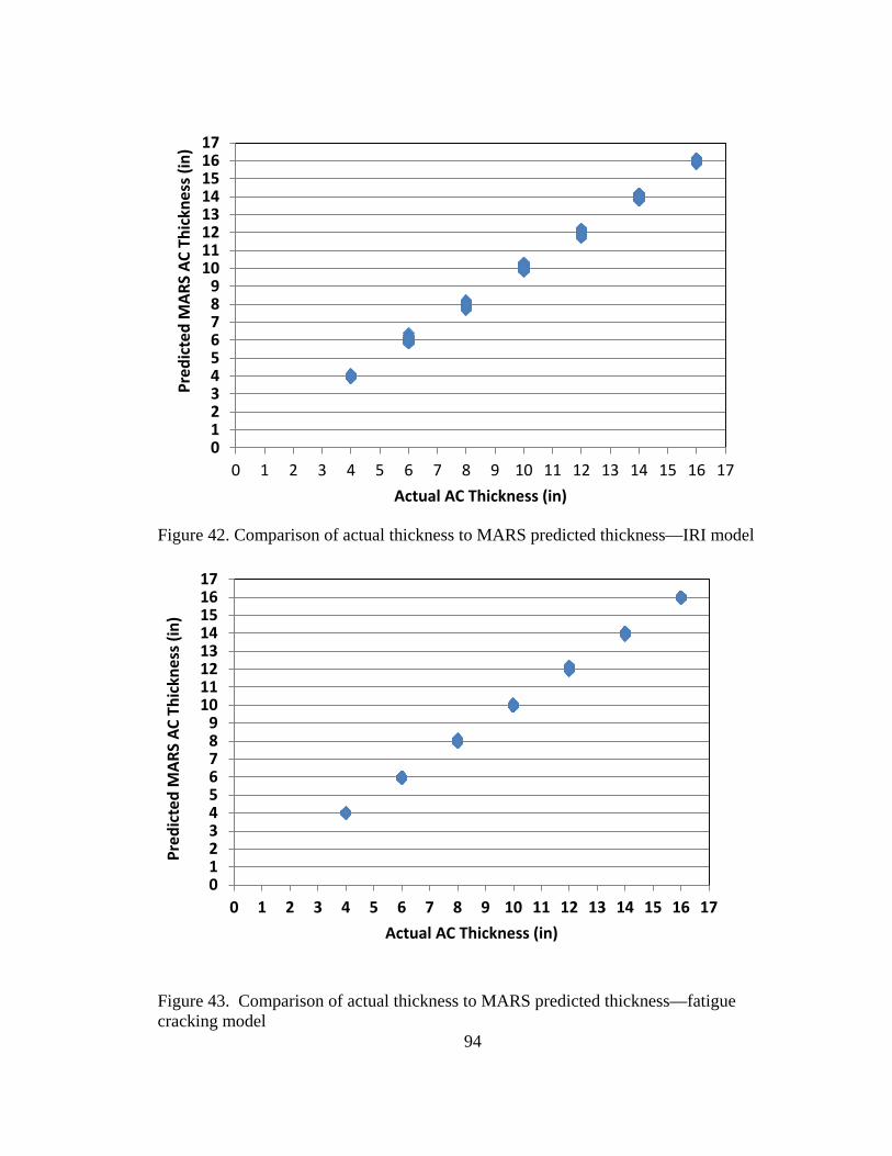
94
Figure 42. Comparison of actual thickness to MARS predicted thickness—IRI model
Figure 43. Comparison of actual thickness to MARS predicted thickness—fatigue cracking model
0123456789
1011121314151617
0 1 2 3 4 5 6 7 8 9 10 11 12 13 14 15 16 17
Pred
icte
d M
ARS
AC T
hick
ness
(in)
Actual AC Thickness (in)
0123456789
1011121314151617
0 1 2 3 4 5 6 7 8 9 10 11 12 13 14 15 16 17
Pred
icte
d M
ARS
AC T
hick
ness
(in)
Actual AC Thickness (in)

95
The actual and predicted thickness agreed very well in the previous figures. As a
means to evaluate the effectiveness of these models another series of MEPDG designs
were developed at various thickness and distress levels which were not included in the
original subset used for model development. These designs were selected across a range
of thicknesses and traffic levels within the overall range of the original MEPDG solutions
used for the model development. The predicted distress results were then input into the
MARS models for each type of distress, providing three predicted thickness results. A
comparison of these predicted thickness for each distress model are shown in Figure 44.
These results illustrate good agreement between the actual and predicted distress for each
distress type.
Figure 44. Comparison of original MEPDG thickness with MARS predicted AC thickness
0123456789
10
0 1 2 3 4 5 6 7 8 9 10MAR
S M
odel
Pre
dict
ed A
spha
lt Th
ickn
ess
(in)
Original MEPDG Asphalt Thickness (in)
Rutting Model IRI Model Fatigue Cracking Model
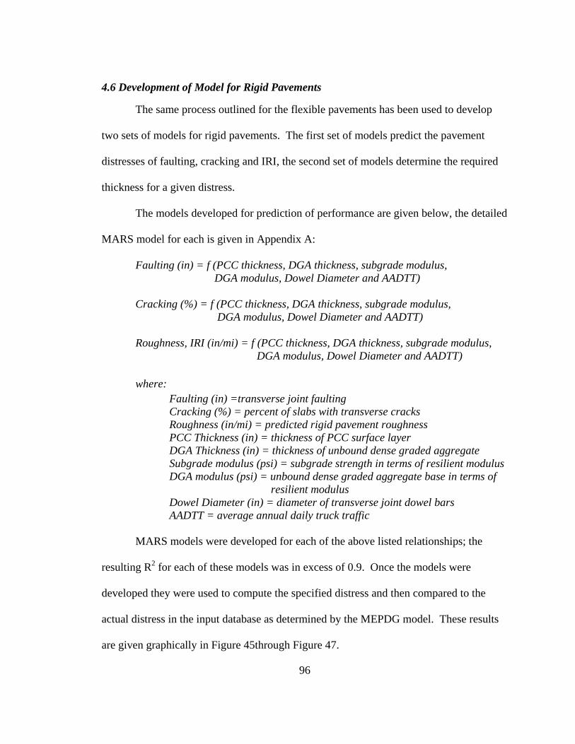
96
4.6 Development of Model for Rigid Pavements
The same process outlined for the flexible pavements has been used to develop
two sets of models for rigid pavements. The first set of models predict the pavement
distresses of faulting, cracking and IRI, the second set of models determine the required
thickness for a given distress.
The models developed for prediction of performance are given below, the detailed
MARS model for each is given in Appendix A:
Faulting (in) = f (PCC thickness, DGA thickness, subgrade modulus, DGA modulus, Dowel Diameter and AADTT) Cracking (%) = f (PCC thickness, DGA thickness, subgrade modulus, DGA modulus, Dowel Diameter and AADTT) Roughness, IRI (in/mi) = f (PCC thickness, DGA thickness, subgrade modulus, DGA modulus, Dowel Diameter and AADTT) where: Faulting (in) =transverse joint faulting Cracking (%) = percent of slabs with transverse cracks Roughness (in/mi) = predicted rigid pavement roughness PCC Thickness (in) = thickness of PCC surface layer DGA Thickness (in) = thickness of unbound dense graded aggregate Subgrade modulus (psi) = subgrade strength in terms of resilient modulus
DGA modulus (psi) = unbound dense graded aggregate base in terms of resilient modulus
Dowel Diameter (in) = diameter of transverse joint dowel bars AADTT = average annual daily truck traffic
MARS models were developed for each of the above listed relationships; the
resulting R2 for each of these models was in excess of 0.9. Once the models were
developed they were used to compute the specified distress and then compared to the
actual distress in the input database as determined by the MEPDG model. These results
are given graphically in Figure 45through Figure 47.

97
The agreement between the distresses calculated using the MEPDG (cracking,
faulting, and IRI) and those predicted by the MARS model is excellent. Cracking is
somewhat clustered above 80 percent level and the below 10 percent level. This is a
function of the sharp break in the distress prediction curve in the MEPDG software. An
example showing the relationship between slab cracking and PCC pavement thickness is
given in Figure 48.
0
0.02
0.04
0.06
0.08
0.1
0.12
0.14
0.16
0 0.02 0.04 0.06 0.08 0.1 0.12 0.14 0.16
Pred
icte
d M
ARS
Faul
ting(
in)
Actual MEPDG Faulting Cracking (in)
Figure 45. Comparison of actual MEPDG faulting with predicted MARS faulting

98
0
10
20
30
40
50
60
70
80
90
100
0 10 20 30 40 50 60 70 80 90 100
Pred
icte
d M
ARS
Slab
Cra
ckin
g (%
)
Actual MEPDG Slab Cracking (%)
Figure 46. Comparison of actual MEPDG slab cracking with predicted MARS slab cracking
50
75
100
125
150
175
200
225
250
50 75 100 125 150 175 200 225 250
Pred
icte
d M
ARS
IRI (
in/m
i)
Actual MEPDG IRI (in/mi)
Figure 47. Comparison of actual MEPDG IRI with predicted MARS IRI

99
In Figure 48 there is a sharp break occurring between seven and nine inches,
depending on the level of traffic. For a pavement thickness less than ten inches the
MEPDG model prediction of slab cracking is very sensitive to pavement thickness, while
above that level it is very insensitive.
As was done for flexible pavements in the previous section an “Efficient Design
Solution” has been developed for rigid pavements utilizing the same concept where the
pavement thicknesses is determined based on a given type of distress. This again gives
the designer the option to select the most conservative design (thickest structure), or
utilize the models developed in the previous section to determine the distress
0
10
20
30
40
50
60
70
80
90
100
6 7 8 9 10 11 12 13 14 15
Slab
s Cra
cked
(%)
PCC Thickness (in)
AADTT 1,000 AADTT 5,000 AADT 10,000 AADTT 15,000 AADTT 25,000
Figure 48. Example of slab cracking model

100
characteristics of each thickness and then choose the design which best fits their design
situation and provides the most efficient design.
The models which make up this “Efficient Design Solution” for rigid pavements
are given below, the detailed MARS model for each is included in Appendix A.
Thickness Faulting Model (in) =
f (Faulting, DGA thickness, subgrade modulus, DGA modulus, Dowel Diameter and AADTT)
Thickness Cracking Model (in) =
f (Cracking, DGA thickness, subgrade modulus, DGA modulus, Dowel Diameter and AADTT)
Thickness Roughness, IRI (in) =
f (IRI, DGA thickness, subgrade modulus, DGA modulus, Dowel Diameter and AADTT)
where: Thickness Faulting Model (in) = calculated PCC thickness -- Faulting Model
Thickness Cracking Model (in) = calculated PCC Thickness – Cracking Mode Thickness Roughness, IRI (in) = calculated PCC Thickness – IRI Model Faulting (in) =transverse joint faulting
Cracking (%) = percent of slabs with transverse cracks Roughness (in/mi) = predicted rigid pavement roughness DGA Thickness (in) = thickness of unbound dense graded aggregate Subgrade modulus (psi) = subgrade strength in terms of resilient modulus
DGA modulus (psi) = unbound dense graded aggregate base in terms of resilient modulus
Dowel Diameter (in) = diameter of transverse joint dowel bars AADTT = average annual daily truck traffic
To evaluate these models the predicted performance results from the subset of
MEPDG solutions were use as input into the MARS models, along with the
corresponding information on traffic and material properties. The thicknesses determined

101
by the models were compared to the actual original input thicknesses used in the MEPDG
predictions. These results are given in Figure 49 through Figure 50.
6
7
8
9
10
11
12
13
14
15
6 7 8 9 10 11 12 13 14 15
Pred
icte
d M
ARS
PCC
Thic
knes
s Iin
)
Actual MEPDG PCC Thickness (in)
Figure 49. Comparison of actual MEPDG thickness with MARS predicted thickness using the slab cracking model

102
6
7
8
9
10
11
12
13
14
15
6 7 8 9 10 11 12 13 14 15
Pred
icte
d M
ARS
PCC
Thic
knes
s Iin
)
Actual MEPDG PCC Thickness (in)
Figure 50. Comparison of actual MEPDG thickness with MARS predicted thickness using the IRI model
6
7
8
9
10
11
12
13
14
15
6 7 8 9 10 11 12 13 14 15
Pred
icte
d M
ARS
PCC
Thic
knes
s Iin
)
Actual MEPDG PCC Thickness (in)
Figure 51. Comparison of actual MEPDG thickness with MARS predicted thickness using the faulting model

103
It may be seen from Figure 49 Figure 50 that the MARS thickness prediction models
have quite bit of variability in the predicted thickness. This variability is generally within
one inch of the target thickness with the exception of a few isolated areas. In Figure 48
the slab-cracking model within the MEPDG has a very sharp break just prior to ten
inches and predicts very little cracking for thicknesses greater than 10 inches. These
very small predicted distress levels, in many cases actually zero, make it very difficult to
accurately predict the design thickness. For example in Figure 48, a level of zero percent
cracking could yield a thickness anywhere from 10 to 14 inches.
To further illustrate the difficulties in predicting pavement thickness for rigid
pavements, an analysis was conducted to look at the MEPDG faulting model results. A
set of calculated faulting results for a given subgrade strength, traffic level, and base
strength is plotted versus pavement thickness at various dowel bar diameters in Figure 52.

104
The faulting models appear to be providing faulting predictions that are not correct.
Specifically for a 1.25-inch diameter dowel, the MEPDG model actually predicts worse
performance as the pavement gets thicker, which is certainly not the case (Figure 52).
Even for 1.5-inch diameter dowel bars for thicknesses less than nine inches the
performance decreases as thickness increases. The effect of this anomaly in the original
MEPDG model can clearly be seen in Figure 50, specifically for thicknesses less than
nine inches.
0.02
0.04
0.06
0.08
0.1
0.12
0.14
0.16
6 7 8 9 10 11 12 13 14 15
Tran
sver
se Jo
int F
aulti
ng (i
n)
PCC Thickness (in)
Dowel Diameter 1.25 Dowel Diameter 1.5 Dowel Diameter 1.75
Figure 52. Example of faulting model

105
5.0 Development of Streamlined Design Process
5.1 Overview of Need for Streamlined Design Process
As has been previously discussed, the most widely used pavement design
procedure in the United States is the AASHTO 1993 pavement design guide. This
procedure has relatively few input parameters and the final result is a thickness of either
Hot-Mix-Asphalt or Portland Cement Concrete. The new NCHRP procedure has many
more potential input parameters and the output is pavement performance, not pavement
thickness. Additional information outlining the individual parameters required for the
NCHRP procedure is contained in Table 1 through Table 4. A comparison of the number
of input requirements for the AASHTO 1993 method and the NCHRP method is given in
Table 19. Depending on the number of layers that are used in the system, the NCHRP
design process could easily have more than 100 input parameters for a single analysis.
Table 19. Summary of Number of Design Inputs
Design Input AASHTO 1993 Number of Inputs Required
Number of Inputs Required NCHRP MEPDG
Climate None three Hot-Mix Asphalt Materials one per layer more than 20 per layer PCC Materials one per layer 1 more than 10 per layer Unbound Materials Granular and Subgrade one per layer eight per layer
Traffic 1 50 Thickness Predicted by Design one per layer
Performance One Reduction in Serviceability (i.e.
performance)
Predicted by Design/Analysis Procedure

106
As has been mentioned the new NCHRP process is an analysis tool and not a
direct design process. A schematic of the process is given in Figure 53.
.
Figure 53. Schematic of NCHRP design/analysis process
This figure illustrates the iterative nature of the NCHRP process, in that design,
thicknesses are assumed, performance is predicted and then an evaluation is made to see
if the design requirements are satisfied.
The concept of an iterative process and the need for a large number of input
parameters (many of which may not be significant) illustrates the need for a streamlined
“Efficient Design Solution” as has been discussed in the previous chapter. This
streamlined procedure will allow a designer to very quickly determine a pavement
thickness and an estimate of the performance of that pavement design in a single step.
InputsTraffic Climate Structure Design Life
Selection of Trial Design
Structural Responses (stress, strain, displacement)
Calibrated Damage-Distress ModelsDistresses Smoothness
Performance VerificationFailure criteria
Design Reliability
Design Requirements
Satisfied? No
Feasible Design
Rev
ise
trial
des
ign
Damage Accumulation with Time
Yes

107
5.2 Comparison of Actual Pavement Design Processes
To illustrate the need of a streamlined design procedure, the following flexible
pavement design scenario will be processed through both the NCHRP Software and the
“Efficient Design Solution” developed during this work. The known design parameters
are given in Table 20.
Table 20. Summary of Pavement Design Inputs
Design Input Value
Average Annual Daily Traffic (AADTT) 14,000
Subgrade Strength (psi) 8,000
Dense Graded Aggregate (DGA) strength (psi) 30,000
Dense Graded Aggregate (DGA) thickness (in) 8.0
Desired Level of Rutting (in) 1.0
Desired Level of Fatigue Cracking (%) 15.0
Desired Level of IRI (in/mi) 150
Since the NCHRP process does not provide any starting point for the designer, they are
left to make assumptions on potential designs based on their experience. These potential
designs are processed through the NCHRP software and the pavement performance is
predicted in terms of fatigue cracking, rutting, and IRI.
To evaluate this design using the NCHRP procedure, potential HMA thickness of
7.25, 9.25, and 11.25 inches were chosen. These thicknesses along with the additional
information provided in Table 20 along with software defaults for the remaining design

108
inputs were processed by the NCHRP software. This software requires approximately
thirty minutes to process each different proposed design thickness. Once the
computational time has been competed the designer will have results as illustrated in
Table 21.
Table 21. Typical NCHRP Process Results
Proposed Thickness (in)
Predicted Fatigue Cracking (%)
Predicted Total Rutting (in)
Predicted IRI (in/mi)
7.25 26.9 1.398 169
9.25 8.62 1.221 150.9
11.25 2.92 1.041 140.8
The designer must now review these results and determine the appropriate design
thickness to meet each of their performance criteria. If none of these results meet the
necessary criteria directly, the designer must now interpolate between the designs to
select the optimum thickness required for each distress.
As was discussed in previous sections, two different sets of MARS models have
been developed during this study. One set of models essentially becomes a surrogate for
the existing NCHRP program, in that they predict pavement performance based on a set
of input values, the second set of models developed the “Efficient Design Solution”
which provides a direct calculation of thickness for a given desired distress. Both of
these sets of models are used to evaluate the design in this example.
Using the design solution developed from the MARS models (“Efficient Design
Solution”), the information contained in Table 20 is used directly to calculate an estimate
of the required thickness for each desired distress. This solution is essentially

109
instantaneous, in that as soon as each input is entered into the procedure, the results are
displayed. The results contain the estimated thickness based on the desired distress and
the predicted performance for this distress. If the procedure were perfect, then the
resulting predicted distress would be exactly what was used to find the estimated
thickness. The results from this procedure are given in Table 22. The predicted distress
levels are very close to the desired distress levels, indicating that the estimated
thicknesses are reasonable estimates which could be used for design and further refined
by the NCHRP process as needed.
Table 22. Pavement Design Results using “Efficient Design Solution”
Distress Desired Level Estimated Thickness
Predicted Distress Level
Fatigue Cracking (%) 15.0 8.0 17
Total Rutting (in) 1.0 11.4 0.98
IRI (in/mi) 150 9.0 151
To illustrate how these designs may compare to those that could be determined
using the full NCHRP process, graphs illustrating the predicted distresses at various
thicknesses were developed. Included in these graphs are the thicknesses which were
estimated using the “Efficient Design Solution” along with their corresponding predicted
distress along with the results from the full MEPDG model. These results are given in
Figure 54 through Figure 56. The designs determined using the “Efficient Design
Solution” are in very good agreement with those from the full NCHRP Procedure.

110
0
5
10
15
20
25
30
6 7 8 9 10 11 12
Fatig
ue C
rack
ing
(%)
HMA Thickness (in) NCHRP MEPDG Results MARS Model Results
Figure 54. Comparison of MEPDG iterations with MARS model prediction, fatigue cracking
0
0.2
0.4
0.6
0.8
1
1.2
1.4
1.6
6 7 8 9 10 11 12
Tota
l Rut
ting
(in)
HMA Thickness (in)
NCHRP MEPDG Results MARS Model Results
Figure 55. Comparison of MEPDG iterations with MARS model prediction, total rutting

111
5.3 Overview of Streamlined Design Process Software
To facilitate the use of the models which have been developed during this work,
an interactive computer program has been developed called “KYPDT”. This software
has been developed using Microsoft Visual Studio as a self-contained software
application. It provides a number of advantages over the NCHRP software. One such
advantage is the direct comparison between the both flexible and rigid pavement designs
for the same design inputs. Using the NCHRP procedure multiple separate designs must
be run for each type of pavement and the comparisons made outside the software
provided.
The NCHRP procedure does not provide any method to directly calculate the cost
any design; this must be done by the designer outside the design process. The solution
70
90
110
130
150
170
190
6 7 8 9 10 11 12
IRI (
in/m
i)
HMA Thickness (in)
NCHRP MEPDG Results MARS Model Results
Figure 56. Comparison of MEPDG iterations with MARS model prediction, IRI

112
developed in this study provides the user the opportunity to input basic cost information
for each material and calculate an estimated total cost based on the estimated thickness
determined for each desired distress. It is anticipated that this program will be utilized by
designers to provide a first estimate of a potential pavement thickness design; they would
then have the option to utilize the full MEPDG model to further refine their design as
necessary. A complete User’s Guide for the software is included in Appendix B.

113
6.0 Summary of Recommendations
6.1 Review of information from Sensitivity Analysis
This study has demonstrated that the global sensitivity analysis is a powerful tool, which
will help to identify potentially important variables for the input parameter studies. It has
also illustrated that default values may be used for the least significant variables and still
achieve acceptable results. It must be kept in mind that the global sensitivity analysis
does not necessarily deal with individual model inputs and how they may impact
individual output values. This method provides a means to screen variables over a wide
range of values and evaluate their relative importance to individual model outputs.
This method has been used successfully to evaluate both flexible and rigid pavement to
identify the most influential variables for which the designer actually has control over or
has the ability to easily determine. This sensitivity analysis did not set out to determine
the sensitivity for every input value within the model, since many of these values are not
readily available in practice.
6.2 Recommended Guidelines for use of Streamlined Model
This study has outlined a method to develop a regression model which can
accurately predict the results of the NCHRP MEPDG software. In addition, an “Efficient
Design Solution” for pavement thickness, given specific distress inputs has been
achieved. The accuracy in these predictions is certainly within acceptable ranges for
initial structural thickness determination, which will make the use of the NCHRP
MEPDG design procedure more efficient due to the reduction in the overall number of
solutions necessary to make a design decision.

114
The new DARWin-ME software (AASHTO, 2011) can facilitate the development
of these subsets through its sensitivity analysis procedure. These sensitivity analysis
solutions can be modeled with the MARS process to produce an “Efficient Design
Solution” of pavement thickness along with a quick prediction of performance for
specific pavement thickness.
Due to the nature of the MARS procedure, models can be easily developed for
any subset of designs necessary, such as typical designs for a state or local agency. This
procedure could be utilized as a replacement for “catalog” designs by providing a method
to determine agency specific designs for any combination of input variables desired or for
the development of very specific design catalogs quickly.
This procedure has the potential to significantly reduce the MEPDG iterations
necessary to develop a viable design, to as few as two to three iterations on either side of
the predicted MARS model thickness. It could then be merged with a smart decision tree
structure to provide very efficient execution of the MEPDG procedure.
The utilization of the streamlined procedure has the potential to provide cost
savings in various areas, including a reduction in the time to complete a potential design,
due to less iteration and less demand for input information which could be costly to
obtain for a wide variety of projects.
The ability for the MARS models to accurately predict the results of the full
MEPDG software provide many advantages to pavement designers. As additional
information becomes available, the MARS models could be expanded to provide

115
performance prediction using various construction quality control results to predict the
change in performance very quickly. This could then be potentially utilized in
performance related specifications.
The MARS models also have the ability to allow for analysis of many different
combinations of variables which can assist in determining potential anomalies in the
MEPDG process as was outlined previously for rigid pavements.
The streamlined model developed in this study is not intended to replace the
NCHRP procedure. Rather it is intended to be a complement to the process by providing
the designer a starting point, or estimated design for which a complete analysis can be
completed using the NCHRP procedure.
6.3 Recommendations for Future Research
The methodologies presented in this study can be expanded to develop very
specific streamlined design processes from a given subset of designs. These methods
could be utilized by agencies who desire to have the robust nature of the NCHRP
MEPDG process, but would like to streamline its use.
One of the more exciting areas where the streamlined model could be expanded is
in the potential for a probabilistic design solution. As was mentioned earlier, this idea
was abandoned in the NCHRP project due to the long computational time required for a
single analysis. By having a model that can be evaluated in seconds, the potential to have
the input values be distributions of likely values and thus providing a distribution of
likely outputs exists. This could provide a means to develop a “true” design reliability

116
based on real variation in input values, instead of relying on the: “surrogate” reliability
that is currently in the NCHRP process.
The continued development of this procedure and subsequent software will open
up the area of mechanistic-empirical design and analysis to a much wider audience. At
the present time the cost of the AASHTO Darwin-ME is approximately $5,000 for a
single user license which could make this procedure somewhat difficult for many
agencies and academic institutions to evaluate.

117
Appendix A -- MARS Models for all Pavement Types

118
MARS Model for HMA Thickness – Fatigue Cracking Model BF1 = Max(0, AADTT - 7500) BF2 = Max(0, 7500 - AADTT) BF3 = Max(0, ALLIGATOR_CRACKING - 1.59) BF4 = Max(0, 1.59 - ALLIGATOR_CRACKING) BF5 = Max(0, SUBGRADE_MODULUS - 9000) BF6 = Max(0, 9000 - SUBGRADE_MODULUS) BF7 = Max(0, DGA_MODULUS - 20000) BF8 = Max(0, AADTT - 2500) BF9 = Max(0, 2500 - AADTT) BF10 = Max(0, DGA_THICKNESS - 10) BF11 = Max(0, 10 - DGA_THICKNESS) BF12 = Max(0, ALLIGATOR_CRACKING - 5.03) * BF8 BF13 = Max(0, 5.03 - ALLIGATOR_CRACKING) * BF8 BF14 = Max(0, ALLIGATOR_CRACKING - 0.6) BF17 = Max(0, 1.15 - ALLIGATOR_CRACKING) * BF9 BF18 = Max(0, ALLIGATOR_CRACKING - 3.29) BF19 = Max(0, 3.29 - ALLIGATOR_CRACKING) BF20 = Max(0, AADTT - 10000) * BF6 BF21 = Max(0, 10000 - AADTT) * BF6 BF22 = Max(0, DGA_THICKNESS - 12) * BF7 BF23 = Max(0, 12 - DGA_THICKNESS) * BF7 BF24 = Max(0, SUBGRADE_MODULUS - 7500) * BF10 BF25 = Max(0, 7500 - SUBGRADE_MODULUS) * BF10 BF26 = Max(0, ALLIGATOR_CRACKING - 0.273) * BF6 BF27 = Max(0, 0.273 - ALLIGATOR_CRACKING) * BF6 BF28 = Max(0, ALLIGATOR_CRACKING - 10.2) * BF5 BF30 = Max(0, ALLIGATOR_CRACKING - 0.907) * BF8 BF31 = Max(0, 0.907 - ALLIGATOR_CRACKING) * BF8 BF32 = Max(0, AADTT - 5000) BF33 = Max(0, 5000 - AADTT) BF34 = Max(0, AADTT - 15000) BF35 = Max(0, 15000 - AADTT) BF36 = Max(0, DGA_THICKNESS - 10) * BF31 BF37 = Max(0, 10 - DGA_THICKNESS) * BF31 BF38 = Max(0, DGA_MODULUS - 30000) * BF31 BF39 = Max(0, 30000 - DGA_MODULUS) * BF31 BF40 = Max(0, SUBGRADE_MODULUS - 10500) * BF11 BF41 = Max(0, 10500 - SUBGRADE_MODULUS) * BF11 BF43 = Max(0, 0.561 - ALLIGATOR_CRACKING) * BF33 BF44 = Max(0, DGA_MODULUS - 30000) * BF6 BF45 = Max(0, 30000 - DGA_MODULUS) * BF6 BF46 = Max(0, ALLIGATOR_CRACKING - 0.409) * BF7
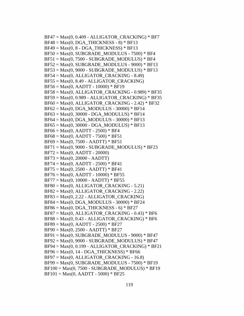
119
BF47 = Max(0, 0.409 - ALLIGATOR_CRACKING) * BF7 BF48 = Max(0, DGA_THICKNESS - 8) * BF13 BF49 = Max(0, 8 - DGA_THICKNESS) * BF13 BF50 = Max(0, SUBGRADE_MODULUS - 7500) * BF4 BF51 = Max(0, 7500 - SUBGRADE_MODULUS) * BF4 BF52 = Max(0, SUBGRADE_MODULUS - 9000) * BF13 BF53 = Max(0, 9000 - SUBGRADE_MODULUS) * BF13 BF54 = Max(0, ALLIGATOR_CRACKING - 8.49) BF55 = Max(0, 8.49 - ALLIGATOR_CRACKING) BF56 = Max(0, AADTT - 10000) * BF19 BF58 = Max(0, ALLIGATOR_CRACKING - 0.989) * BF35 BF59 = Max(0, 0.989 - ALLIGATOR_CRACKING) * BF35 BF60 = Max(0, ALLIGATOR_CRACKING - 2.42) * BF32 BF62 = Max(0, DGA_MODULUS - 30000) * BF14 BF63 = Max(0, 30000 - DGA_MODULUS) * BF14 BF64 = Max(0, DGA_MODULUS - 30000) * BF13 BF65 = Max(0, 30000 - DGA_MODULUS) * BF13 BF66 = Max(0, AADTT - 2500) * BF4 BF68 = Max(0, AADTT - 7500) * BF51 BF69 = Max(0, 7500 - AADTT) * BF51 BF71 = Max(0, 9000 - SUBGRADE_MODULUS) * BF23 BF72 = Max(0, AADTT - 20000) BF73 = Max(0, 20000 - AADTT) BF74 = Max(0, AADTT - 2500) * BF41 BF75 = Max(0, 2500 - AADTT) * BF41 BF76 = Max(0, AADTT - 10000) * BF55 BF77 = Max(0, 10000 - AADTT) * BF55 BF80 = Max(0, ALLIGATOR_CRACKING - 5.21) BF82 = Max(0, ALLIGATOR_CRACKING - 2.22) BF83 = Max(0, 2.22 - ALLIGATOR_CRACKING) BF84 = Max(0, DGA_MODULUS - 30000) * BF24 BF86 = Max(0, DGA_THICKNESS - 6) * BF27 BF87 = Max(0, ALLIGATOR_CRACKING - 0.43) * BF6 BF88 = Max(0, 0.43 - ALLIGATOR_CRACKING) * BF6 BF89 = Max(0, AADTT - 2500) * BF27 BF90 = Max(0, 2500 - AADTT) * BF27 BF91 = Max(0, SUBGRADE_MODULUS - 9000) * BF47 BF92 = Max(0, 9000 - SUBGRADE_MODULUS) * BF47 BF94 = Max(0, 0.199 - ALLIGATOR_CRACKING) * BF21 BF96 = Max(0, 14 - DGA_THICKNESS) * BF66 BF97 = Max(0, ALLIGATOR_CRACKING - 16.8) BF99 = Max(0, SUBGRADE_MODULUS - 7500) * BF19 BF100 = Max(0, 7500 - SUBGRADE_MODULUS) * BF19 BF101 = Max(0, AADTT - 5000) * BF25
120
BF102 = Max(0, 5000 - AADTT) * BF25 BF104 = Max(0, 0.723 - ALLIGATOR_CRACKING) * BF71 BF105 = Max(0, DGA_MODULUS - 30000) * BF102 BF107 = Max(0, SUBGRADE_MODULUS - 7500) * BF96 BF108 = Max(0, 7500 - SUBGRADE_MODULUS) * BF96 BF109 = Max(0, DGA_THICKNESS - 8) * BF83 BF110 = Max(0, 8 - DGA_THICKNESS) * BF83 BF111 = Max(0, SUBGRADE_MODULUS - 10500) * BF19 BF112 = Max(0, 10500 - SUBGRADE_MODULUS) * BF19 BF113 = Max(0, AADTT - 5000) * BF91 BF114 = Max(0, 5000 - AADTT) * BF91 BF116 = Max(0, 0.428 - ALLIGATOR_CRACKING) * BF25 BF118 = Max(0, 30000 - DGA_MODULUS) * BF35 BF120 = Max(0, 1.23 - ALLIGATOR_CRACKING) * BF73 BF121 = Max(0, AADTT - 2500) * BF83 BF122 = Max(0, 2500 - AADTT) * BF83 BF123 = Max(0, DGA_MODULUS - 20000) * BF52 BF124 = Max(0, DGA_THICKNESS - 14) * BF53 BF125 = Max(0, 14 - DGA_THICKNESS) * BF53 BF126 = Max(0, AADTT - 20000) * BF112 BF127 = Max(0, 20000 - AADTT) * BF112 BF128 = Max(0, AADTT - 2500) * BF10 BF129 = Max(0, 2500 - AADTT) * BF10 BF130 = Max(0, DGA_THICKNESS - 8) * BF7 BF132 = Max(0, DGA_MODULUS - 20000) * BF121 BF133 = Max(0, DGA_THICKNESS - 14) BF135 = Max(0, AADTT - 7500) * BF88 BF136 = Max(0, 7500 - AADTT) * BF88 BF137 = Max(0, AADTT - 2500) * BF5 BF138 = Max(0, 2500 - AADTT) * BF5 BF139 = Max(0, ALLIGATOR_CRACKING - 1.64) * BF34 BF141 = Max(0, ALLIGATOR_CRACKING - 3.95) BF143 = Max(0, ALLIGATOR_CRACKING - 6.43) * BF8 BF145 = Max(0, AADTT - 7500) * BF27 BF148 = Max(0, 1.23 - ALLIGATOR_CRACKING) * BF20 BF149 = Max(0, SUBGRADE_MODULUS - 7500) * BF39 BF150 = Max(0, 7500 - SUBGRADE_MODULUS) * BF39 allcrack_drain_0 = 13.1355 + 0.00113966 * BF1 - 0.00122041 * BF2 - 3.74709 * BF3 + 4.14962 * BF4 - 0.000068255 * BF5 + 0.000296141 * BF6 - 0.0000708209 * BF7 - 0.00138207 * BF8 - 0.0727677 * BF10 + 0.0781646 * BF11 - 0.00014892 * BF12 + 0.000151419 * BF13 + 2.18065 * BF14 - 0.000113179 * BF17 + 0.212216 * BF18 + 0.0000000047076 * BF20 - 0.00000000850912 * BF21 - 0.00000362552 * BF22 + 0.00000445556 * BF23 + 0.000005184 * BF24 - 0.0000207563 * BF25

121
- 0.000966547 * BF26 + 0.00160266 * BF27 + 0.00000781016 * BF28 + 0.000154065 * BF30 - 0.000182606 * BF32 - 0.0000510239 * BF34 - 0.00000662715 * BF36 + 0.0000136714 * BF37 - 0.00000000186975 * BF38 + 0.00000000599187 * BF39 - 0.00000448542 * BF40 + 0.0000103693 * BF41 - 0.000275742 * BF43 - 0.00000000323229 * BF44 + 0.0000000037792 * BF45 + 0.0000335673 * BF46 + 0.000141792 * BF47 - 0.00000029566 * BF48 + 0.000000644883 * BF49 - 0.0000324771 * BF50 + 0.0000638516 * BF51 - 0.000000000818329 * BF52 - 0.00000000104293 * BF53 + 0.104811 * BF54 + 0.00000285529 * BF56 + 0.0000179223 * BF58 + 0.0000260377 * BF59 + 0.0000104522 * BF60 - 0.0000334501 * BF62 + 0.000033906 * BF63 - 9.96897E-11 * BF64 + 0.00000000023986 * BF65 + 0.0000224086 * BF66 - 0.00000000669878 * BF68 - 0.0000000213097 * BF69 + 0.000000000253166 * BF71 - 0.0000215622 * BF72 + 0.0000000001621 * BF74 - 0.00000000221213 * BF75 - 0.00000295211 * BF76 - 0.00000582606 * BF77 + 0.0912604 * BF80 + 0.350733 * BF82 + 0.000000000237907 * F84 + 0.0000633759 * BF86 + 0.000955862 * BF87 + 0.000000261164 * BF89 - 0.000000134052 * BF90 - 0.0000000563975 * BF91 - 0.0000000508487 * BF92 + 0.00000023726 * BF94 + 0.00000320634 * BF96 + 0.0519829 * BF97 - 0.0000272267 * BF99 + 0.0000744313 * BF100 + 0.000000000817261 * BF101 + 0.00000000312414 * BF102 + 0.00000000131106 * BF104 + 7.0961E-13 * BF105 - 0.000000000693289 * BF107 - 0.00000000154212 * BF108 - 0.00486935 * BF109 + 0.00952931 * BF110 + 0.000030758 * BF111 + 1.07041E-11 * BF113 + 1.17895E-11 * BF114 - 0.000102005 * BF116 + 0.000000000240567 * BF118 + 0.0000237499 * BF120 - 0.00008349 * BF122 + 3.08638E-14 * BF123 - 0.00000000015773 * BF124 + 0.000000000200888 * BF125 + 0.000000000745265 * BF126 - 0.00000000148787 * BF127 - 0.000000239459 * BF128 + 0.00000402042 * BF129 + 0.00000147312 * BF130 - 0.000000000299643 * BF132 + 0.0145845 * BF133 + 0.000000103081 * BF135 - 0.00000003695 * BF136 - 0.000000000809332 * BF137 + 0.0000000104058 * BF138 - 0.0000208569 * BF139 + 0.0980544 * BF141 + 0.00000322751 * BF143 - 0.000000360997 * BF145 + 0.00000000991327 * BF148 - 1.16614E-12 * BF149 - 1.1454E-12 * BF150

122
MARS Model for HMA Thickness – IRI Model BF1 = Max(0, AADTT - 7500) BF2 = Max(0, 7500 - AADTT) BF3 = Max(0, IRI - 135.2) BF4 = Max(0, 135.2 - IRI) BF5 = Max(0, SUBGRADE_MODULUS - 7500) BF6 = Max(0, 7500 - SUBGRADE_MODULUS) BF7 = Max(0, AADTT - 2500) * BF4 BF8 = Max(0, 2500 - AADTT) * BF4 BF9 = Max(0, IRI - 124.5) * BF2 BF10 = Max(0, 124.5 - IRI) * BF2 BF12 = Max(0, 7500 - SUBGRADE_MODULUS) * BF1 BF13 = Max(0, DGA_MODULUS - 20000) BF14 = Max(0, AADTT - 5000) * BF4 BF15 = Max(0, 5000 - AADTT) * BF4 BF16 = Max(0, AADTT - 10000) BF17 = Max(0, 10000 - AADTT) BF19 = Max(0, 12000 - SUBGRADE_MODULUS) * BF15 BF20 = Max(0, IRI - 119.3) * BF17 BF21 = Max(0, 119.3 - IRI) * BF17 BF22 = Max(0, AADTT - 5000) * BF13 BF23 = Max(0, 5000 - AADTT) * BF13 BF24 = Max(0, IRI - 129.2) * BF12 BF25 = Max(0, 129.2 - IRI) * BF12 BF26 = Max(0, IRI - 152.4) * BF5 BF27 = Max(0, 152.4 - IRI) * BF5 BF28 = Max(0, DGA_THICKNESS - 6) * BF23 BF29 = Max(0, AADTT - 20000) BF30 = Max(0, 20000 - AADTT) BF31 = Max(0, IRI - 122.8) BF32 = Max(0, 122.8 - IRI) BF33 = Max(0, SUBGRADE_MODULUS - 7500) * BF14 BF34 = Max(0, 7500 - SUBGRADE_MODULUS) * BF14 BF35 = Max(0, SUBGRADE_MODULUS - 9000) * BF17 BF36 = Max(0, 9000 - SUBGRADE_MODULUS) * BF17 BF37 = Max(0, IRI - 132.4) * BF35 BF38 = Max(0, 132.4 - IRI) * BF35 BF39 = Max(0, AADTT - 5000) BF40 = Max(0, 5000 - AADTT) BF41 = Max(0, AADTT - 2500) * BF5 BF42 = Max(0, 2500 - AADTT) * BF5 BF43 = Max(0, IRI - 126.3) * BF6 BF44 = Max(0, 126.3 - IRI) * BF6

123
BF45 = Max(0, AADTT - 5000) * BF44 BF46 = Max(0, 5000 - AADTT) * BF44 BF47 = Max(0, AADTT - 5000) * BF6 BF48 = Max(0, 5000 - AADTT) * BF6 BF49 = Max(0, DGA_MODULUS - 20000) * BF25 BF50 = Max(0, DGA_THICKNESS - 6) * BF34 BF51 = Max(0, DGA_MODULUS - 30000) * BF45 BF52 = Max(0, 30000 - DGA_MODULUS) * BF45 BF53 = Max(0, AADTT - 10000) * BF6 BF54 = Max(0, 10000 - AADTT) * BF6 BF55 = Max(0, DGA_MODULUS - 30000) * BF31 BF56 = Max(0, 30000 - DGA_MODULUS) * BF31 BF57 = Max(0, SUBGRADE_MODULUS - 12000) * BF20 BF58 = Max(0, 12000 - SUBGRADE_MODULUS) * BF20 BF59 = Max(0, AADTT - 20000) * BF31 BF60 = Max(0, 20000 - AADTT) * BF31 BF61 = Max(0, DGA_THICKNESS - 6) * BF45 BF62 = Max(0, SUBGRADE_MODULUS - 10500) * BF39 BF63 = Max(0, 10500 - SUBGRADE_MODULUS) * BF39 BF64 = Max(0, IRI - 136.9) * BF41 BF65 = Max(0, 136.9 - IRI) * BF41 BF66 = Max(0, DGA_THICKNESS - 12) * BF27 BF67 = Max(0, 12 - DGA_THICKNESS) * BF27 BF68 = Max(0, DGA_THICKNESS - 6) * BF49 BF69 = Max(0, DGA_THICKNESS - 10) * BF30 BF70 = Max(0, 10 - DGA_THICKNESS) * BF30 BF71 = Max(0, IRI - 117.4) * BF23 BF72 = Max(0, 117.4 - IRI) * BF23 BF73 = Max(0, SUBGRADE_MODULUS - 10500) * BF60 BF74 = Max(0, 10500 - SUBGRADE_MODULUS) * BF60 BF75 = Max(0, AADTT - 15000) * BF27 BF77 = Max(0, IRI - 128.7) * BF42 BF78 = Max(0, 128.7 - IRI) * BF42 BF79 = Max(0, IRI - 126.8) * BF40 BF81 = Max(0, AADTT - 2500) * BF32 BF82 = Max(0, 2500 - AADTT) * BF32 BF83 = Max(0, DGA_THICKNESS - 12) * BF8 BF84 = Max(0, 12 - DGA_THICKNESS) * BF8 BF85 = Max(0, DGA_MODULUS - 30000) * BF69 BF86 = Max(0, 30000 - DGA_MODULUS) * BF69 BF87 = Max(0, IRI - 130.2) * BF23 BF89 = Max(0, DGA_THICKNESS - 6) * BF10 BF90 = Max(0, IRI - 125.5) * BF6 BF91 = Max(0, 125.5 - IRI) * BF6
124
BF92 = Max(0, AADTT - 5000) * BF91 BF94 = Max(0, DGA_MODULUS - 30000) * BF92 BF95 = Max(0, 30000 - DGA_MODULUS) * BF92 BF96 = Max(0, DGA_MODULUS - 30000) * BF61 BF97 = Max(0, 30000 - DGA_MODULUS) * BF61 BF98 = Max(0, DGA_MODULUS - 30000) * BF8 BF99 = Max(0, 30000 - DGA_MODULUS) * BF8 BF100 = Max(0, DGA_THICKNESS - 8) * BF3 BF101 = Max(0, 8 - DGA_THICKNESS) * BF3 BF102 = Max(0, SUBGRADE_MODULUS - 7500) * BF81 BF103 = Max(0, 7500 - SUBGRADE_MODULUS) * BF81 BF104 = Max(0, AADTT - 2500) * BF91 BF105 = Max(0, 2500 - AADTT) * BF91 BF106 = Max(0, SUBGRADE_MODULUS - 7500) * BF21 BF109 = Max(0, 7500 - SUBGRADE_MODULUS) * BF69 BF110 = Max(0, DGA_MODULUS - 30000) * BF2 BF111 = Max(0, 30000 - DGA_MODULUS) * BF2 BF112 = Max(0, SUBGRADE_MODULUS - 9000) * BF82 BF113 = Max(0, 9000 - SUBGRADE_MODULUS) * BF82 BF114 = Max(0, IRI - 138.4) * BF5 BF115 = Max(0, 138.4 - IRI) * BF5 BF116 = Max(0, SUBGRADE_MODULUS - 10500) * BF23 BF117 = Max(0, 10500 - SUBGRADE_MODULUS) * BF23 BF118 = Max(0, IRI - 122.6) * BF54 BF119 = Max(0, 122.6 - IRI) * BF54 BF120 = Max(0, IRI - 123.7) * BF54 BF122 = Max(0, DGA_MODULUS - 20000) * BF70 BF125 = Max(0, IRI - 137.7) * BF22 BF126 = Max(0, 137.7 - IRI) * BF22 BF127 = Max(0, AADTT - 2500) * BF67 BF128 = Max(0, 2500 - AADTT) * BF67 BF129 = Max(0, AADTT - 15000) * BF13 BF131 = Max(0, DGA_THICKNESS - 6) * BF9 BF132 = Max(0, IRI - 129) * BF2 BF134 = Max(0, IRI - 117.5) * BF69 BF135 = Max(0, 117.5 - IRI) * BF69 BF136 = Max(0, AADTT - 15000) * BF100 BF138 = Max(0, IRI - 122.8) * BF54 BF140 = Max(0, SUBGRADE_MODULUS - 9000) BF141 = Max(0, 9000 - SUBGRADE_MODULUS) BF142 = Max(0, AADTT - 15000) * BF141 BF143 = Max(0, 15000 - AADTT) * BF141 BF144 = Max(0, SUBGRADE_MODULUS - 10500) * BF30 BF145 = Max(0, 10500 - SUBGRADE_MODULUS) * BF30

125
BF146 = Max(0, DGA_THICKNESS - 14) * BF141 BF147 = Max(0, 14 - DGA_THICKNESS) * BF141 BF148 = Max(0, IRI - 157.7) * BF140 BF149 = Max(0, 157.7 - IRI) * BF140 BF150 = Max(0, AADTT - 500) * BF115 IRI_Draini_0 = 10.2431 + 0.000956761 * BF1 - 0.00121258 * BF2 - 0.329257 * BF3 + 0.37384 * BF4 - 0.00187586 * BF5 + 0.00110821 * BF6 - 0.00000585863 * BF7 - 0.000131539 * BF8 + 0.00000367024 * BF9 + 0.00000129877 * BF12 - 0.00000508463 * BF13 - 0.000230611 * BF16 + 0.000000000640121 * BF19 + 0.0000181612 * BF20 + 0.0000400117 * BF21 + 0.00000000186738 * BF22 + 0.000000000805772 * BF24 - 0.0000680218 * BF26 + 0.0000904455 * BF27 - 0.000000000459619 * BF28 - 0.000139161 * BF29 + 0.125606 * BF31 - 0.00000000325205 * BF33 - 0.00000010445 * BF35 + 0.000000164859 * BF36 + 0.00000000684486 * BF37 - 0.00000000359774 * BF38 - 0.000429299 * BF39 + 0.000000123827 * BF42 + 0.00046961 * BF43 + 0.000569872 * BF44 - 0.0000000483349 * BF45 - 0.000000415091 * BF46 - 0.000000686603 * BF47 + 0.0000000854554 * BF48 - 5.70313E-13 * BF49 - 7.73792E-11 * BF50 - 4.91131E-12 * BF51 + 1.17614E-11 * BF52 - 0.000000590413 * BF53 - 0.00000135468 * BF55 + 0.00000157488 * BF56 + 0.00000000746813 * BF57 - 0.00000000692815 * BF58 + 0.00000404208 * BF59 - 0.00000102236 * BF60 - 0.0000000080072 * BF61 + 0.0000000398633 * BF62 - 0.0000000368262 * BF63 - 0.00000000231371 * BF64 - 0.00000000248158 * BF65 + 0.000000159309 * BF66 - 0.000000107885 * BF67 - 1.28336E-13 * BF68 - 0.00000092758 * BF69 - 8.32453E-11 * BF71 + 0.00000000190864 * BF72 + 0.000000000857133 * BF73 - 0.000000000708659 * BF74 - 0.00000000213034 * BF75 - 0.000000028809 * BF77 + 0.00000000441369 * BF78 + 0.0000293637 * BF79 - 0.0000637828 * BF81 - 0.0000198705 * BF82 - 0.0000016848 * BF83 + 0.00000247618 * BF84 - 2.73409E-11 * BF85 + 9.80311E-11 * BF86 + 0.00000000219391 * BF87 + 0.000000860885 * BF89 - 0.000471098 * BF90 + 0.00000107695 * BF92 + 2.27258E-12 * BF94 - 0.0000000000118 * BF95 - 2.80104E-13 * BF96 + 6.89492E-13 * BF97 - 0.000000000607294 * BF98 + 0.000000000499643 * BF99 - 0.000890849 * BF100 + 0.002564 * BF101 + 0.0000000108428 * BF102 + 0.000000190378 * BF103 - 0.00000050842 * BF104 + 0.000000429713 * BF105 - 0.00000000830773 * BF106 - 0.000000000277217 * BF109 - 0.00000000163059 * BF110 + 0.00000000311248 * BF111 - 0.0000000107599 * BF112 + 0.0000000385213 * BF113 + 0.000120361 * BF114 - 2.73344E-13 * BF116 + 4.19601E-13 * BF117- 0.0000000879177 * BF118 + 0.0000000371198 * BF119 + 0.000000194454 * BF120 + 8.36832E-11 * BF122 + 3.33084E-11 * BF125 - 0.000000000108579 * BF126 - 1.33202E-11 * BF127 - 6.71344E-11 * BF128 - 0.00000000138799 * BF129 - 0.000000902901 * BF131 + 0.0000193757 * BF132 + 0.0000000742015 * BF134 + 0.000000637464 * BF135 + 0.000000129692 * BF136 - 0.0000000982426 * BF138 + 0.0000603609 * BF140

126
- 0.00000000748308 * BF142 - 0.0000000222126 * BF143 - 0.0000000126426 * BF144 + 0.0000000158054 * BF145 - 0.00000642383 * BF146 + 0.00000194495 * BF147 + 0.0000074903 * BF148 + 0.00000220845 * BF149 - 0.00000000421066 * BF150

127
MARS Model for HMA Thickness – Total Rutting Model BF1 = Max(0, AADTT - 7500) BF2 = Max(0, 7500 - AADTT) BF3 = Max(0, total_rutting - 0.579) BF4 = Max(0, 0.579 - total_rutting) BF5 = Max(0, SUBGRADE_MODULUS - 7500) BF6 = Max(0, 7500 - SUBGRADE_MODULUS) BF7 = Max(0, AADTT - 2500) BF8 = Max(0, 2500 - AADTT) BF9 = Max(0, SUBGRADE_MODULUS - 9000) * BF7 BF10 = Max(0, 9000 - SUBGRADE_MODULUS) * BF7 BF11 = Max(0, AADTT - 10000) * BF3 BF12 = Max(0, 10000 - AADTT) * BF3 BF13 = Max(0, AADTT - 5000) BF14 = Max(0, 5000 - AADTT) BF15 = Max(0, DGA_MODULUS - 30000) * BF2 BF16 = Max(0, 30000 - DGA_MODULUS) * BF2 BF17 = Max(0, total_rutting - 0.634) * BF5 BF18 = Max(0, 0.634 - total_rutting) * BF5 BF19 = Max(0, total_rutting - 0.552) * BF8 BF20 = Max(0, 0.552 - total_rutting) * BF8 BF21 = Max(0, AADTT - 20000) * BF5 BF22 = Max(0, 20000 - AADTT) * BF5 BF23 = Max(0, total_rutting - 0.703) * BF14 BF24 = Max(0, 0.703 - total_rutting) * BF14 BF25 = Max(0, DGA_THICKNESS - 6) * BF17 BF26 = Max(0, total_rutting - 0.774) * BF10 BF27 = Max(0, 0.774 - total_rutting) * BF10 BF29 = Max(0, 9000 - SUBGRADE_MODULUS) * BF14 BF30 = Max(0, total_rutting - 0.692) * BF2 BF31 = Max(0, 0.692 - total_rutting) * BF2 BF32 = Max(0, DGA_THICKNESS - 6) * BF15 BF33 = Max(0, AADTT - 15000) BF34 = Max(0, 15000 - AADTT) BF35 = Max(0, total_rutting - 0.822) BF36 = Max(0, 0.822 - total_rutting) BF37 = Max(0, SUBGRADE_MODULUS - 9000) * BF36 BF38 = Max(0, 9000 - SUBGRADE_MODULUS) * BF36 BF40 = Max(0, 2500 - AADTT) * BF37 BF41 = Max(0, DGA_MODULUS - 20000) * BF27 BF42 = Max(0, total_rutting - 0.719) * BF10 BF43 = Max(0, 0.719 - total_rutting) * BF10 BF44 = Max(0, AADTT - 7500) * BF38 BF45 = Max(0, 7500 - AADTT) * BF38

128
BF46 = Max(0, AADTT - 10000) * BF6 BF47 = Max(0, 10000 - AADTT) * BF6 BF48 = Max(0, SUBGRADE_MODULUS - 7500) * BF34 BF49 = Max(0, 7500 - SUBGRADE_MODULUS) * BF34 BF50 = Max(0, DGA_THICKNESS - 6) * BF38 BF53 = Max(0, total_rutting - 1.062) BF55 = Max(0, SUBGRADE_MODULUS - 10500) * BF12 BF56 = Max(0, 10500 - SUBGRADE_MODULUS) * BF12 BF57 = Max(0, AADTT - 5000) * BF6 BF60 = Max(0, 20000 - AADTT) * BF35 BF61 = Max(0, DGA_MODULUS - 30000) * BF44 BF62 = Max(0, 30000 - DGA_MODULUS) * BF44 BF63 = Max(0, total_rutting - 0.576) * BF29 BF64 = Max(0, 0.576 - total_rutting) * BF29 BF65 = Max(0, SUBGRADE_MODULUS - 9000) * BF2 BF66 = Max(0, 9000 - SUBGRADE_MODULUS) * BF2 BF67 = Max(0, total_rutting - 0.728) * BF49 BF69 = Max(0, total_rutting - 0.689) * BF6 BF70 = Max(0, 0.689 - total_rutting) * BF6 BF71 = Max(0, DGA_THICKNESS - 6) * BF41 BF73 = Max(0, 10500 - SUBGRADE_MODULUS) * BF30 BF74 = Max(0, DGA_THICKNESS - 6) BF75 = Max(0, AADTT - 2500) * BF74 BF76 = Max(0, 2500 - AADTT) * BF74 BF77 = Max(0, DGA_MODULUS - 30000) * BF76 BF78 = Max(0, 30000 - DGA_MODULUS) * BF76 BF79 = Max(0, total_rutting - 0.481) * BF74 BF80 = Max(0, 0.481 - total_rutting) * BF74 BF81 = Max(0, SUBGRADE_MODULUS - 12000) * BF74 BF82 = Max(0, 12000 - SUBGRADE_MODULUS) * BF74 BF83 = Max(0, AADTT - 10000) * BF38 BF85 = Max(0, DGA_MODULUS - 30000) * BF74 BF86 = Max(0, 30000 - DGA_MODULUS) * BF74 BF87 = Max(0, DGA_MODULUS - 30000) * BF43 BF88 = Max(0, 30000 - DGA_MODULUS) * BF43 BF89 = Max(0, total_rutting - 0.662) * BF6 BF91 = Max(0, total_rutting - 0.728) * BF47 BF92 = Max(0, 0.728 - total_rutting) * BF47 BF93 = Max(0, total_rutting - 0.678) * BF29 BF95 = Max(0, SUBGRADE_MODULUS - 12000) * BF24 BF96 = Max(0, 12000 - SUBGRADE_MODULUS) * BF24 BF97 = Max(0, AADTT - 5000) * BF85 BF98 = Max(0, 5000 - AADTT) * BF85 BF100 = Max(0, 1.253 - total_rutting) * BF86

129
BF101 = Max(0, total_rutting - 0.687) * BF32 BF103 = Max(0, total_rutting - 0.629) * BF22 BF104 = Max(0, 0.629 - total_rutting) * BF22 BF105 = Max(0, SUBGRADE_MODULUS - 9000) * BF11 BF106 = Max(0, 9000 - SUBGRADE_MODULUS) * BF11 BF107 = Max(0, SUBGRADE_MODULUS - 7500) * BF79 BF108 = Max(0, 7500 - SUBGRADE_MODULUS) * BF79 BF109 = Max(0, SUBGRADE_MODULUS - 12000) BF112 = Max(0, 12 - DGA_THICKNESS) * BF14 BF113 = Max(0, total_rutting - 0.497) * BF112 BF114 = Max(0, 0.497 - total_rutting) * BF112 BF116 = Max(0, 10500 - SUBGRADE_MODULUS) * BF16 BF117 = Max(0, DGA_THICKNESS - 10) * BF43 BF118 = Max(0, 10 - DGA_THICKNESS) * BF43 BF119 = Max(0, DGA_THICKNESS - 10) * BF27 BF121 = Max(0, total_rutting - 1.214) * BF7 BF124 = Max(0, 7500 - SUBGRADE_MODULUS) * BF86 BF125 = Max(0, AADTT - 7500) * BF50 BF126 = Max(0, 7500 - AADTT) * BF50 BF127 = Max(0, DGA_MODULUS - 30000) * BF17 BF128 = Max(0, 30000 - DGA_MODULUS) * BF17 BF129 = Max(0, AADTT - 7500) * BF124 BF130 = Max(0, 7500 - AADTT) * BF124 BF131 = Max(0, DGA_THICKNESS - 10) * BF18 BF132 = Max(0, 10 - DGA_THICKNESS) * BF18 BF133 = Max(0, SUBGRADE_MODULUS - 10500) * BF75 BF134 = Max(0, 10500 - SUBGRADE_MODULUS) * BF75 BF135 = Max(0, DGA_MODULUS - 20000) * BF8 BF137 = Max(0, 7500 - AADTT) * BF128 BF138 = Max(0, AADTT - 15000) * BF124 BF140 = Max(0, DGA_THICKNESS - 6) * BF88 BF142 = Max(0, 30000 - DGA_MODULUS) * BF14 BF143 = Max(0, DGA_MODULUS - 20000) * BF67 BF144 = Max(0, total_rutting - 0.703) BF146 = Max(0, SUBGRADE_MODULUS - 10500) BF148 = Max(0, total_rutting - 0.461) * BF135 BF149 = Max(0, 0.461 - total_rutting) * BF135 BF150 = Max(0, DGA_THICKNESS - 6) * BF87 totalrut_drain_0 = 28.1067 + 0.00329821 * BF1 - 0.00350442 * BF2 - 8.45495 * BF3 + 14.8171 * BF4 - 0.0029254 * BF5 - 0.00366096 * BF6 - 0.00215979 * BF7 + 0.000000163066 * BF9 - 0.000000496841 * BF10 + 0.000321779 * BF11 - 0.00103076 * BF12 - 0.000723493 * BF13 - 0.00000000191416 * BF15 - 0.000657002 * BF17 - 0.00140932 * BF18 + 0.00809587 * BF19 - 0.00273971 * BF20

130
- 0.000000174914 * BF21 + 0.000000145272 * BF22 + 0.00209759 * BF23 + 0.000435807 * BF24 + 0.000123695 * BF25 - 0.00000613233 * BF26 + 0.00000303238 * BF27 + 0.000000208601 * BF29 - 0.000707227 * BF30 + 0.000965066 * BF31 + 0.000000000628148 * BF32 - 0.000161857 * BF33 + 0.000360048 * BF37 - 0.00163343 * BF38 - 0.000000250937 * BF40 - 3.76474E-11 * BF41 + 0.00000616447 * BF42 + 0.00000147555 * BF44 - 0.00000227987 * BF45 - 0.000000722238 * BF46 - 0.000000110167 * BF47 + 0.00000000427238 * BF48 + 0.000000455174 * BF49 - 0.0000428305 * BF50 - 1.83169 * BF53 - 0.0000000670946 * BF55 + 0.000000135158 * BF56 + 0.000000894616 * BF57 - 0.000254134 * BF60 + 1.19295E-11 * BF61 - 1.18937E-11 * BF62 - 0.00000442253 * BF63 + 0.00000399545 * BF64 - 0.000000014337 * BF65 + 0.000000526511 * BF66 - 0.0000426377 * BF67 - 0.0198867 * BF69 + 0.0293042 * BF70 - 4.57047E-12 * BF71 - 0.000000343313 * BF73 + 0.0947603 * BF74 - 0.00000120411 * BF75 - 0.0000300161 * BF76 - 0.00000000038338 * BF77 + 0.00000000110166 * BF78 + 0.0689348 * BF79 + 1.11562 * BF80 + 0.0000219319 * BF81 - 0.0000237441 * BF82 - 0.00000253145 * BF83- 0.00000117232 * BF85 + 4.24832E-11 * BF87 - 3.52057E-11 * BF88 + 0.0204752 * BF89 + 0.0000756819 * BF91 - 0.00000331816 * BF92 - 0.00000559208 * BF93 - 0.000000245808 * BF95 + 0.000000360106 * BF96 + 4.55699E-11 * BF97 - 0.00000000141391 * BF98 + 0.00000322256 * BF100 - 0.00000000677274 * BF101 + 0.0000000473393 * BF103 + 0.0000000700681 * BF104 + 0.000000031683 * BF105 - 0.0000000730102 * BF106 - 0.00011908 * BF107 + 0.0000188122 * BF108 + 0.0000425199 * BF109 + 0.000039193 * BF113 + 0.000136233 * BF114 - 3.9875E-13 * BF116 + 0.000000143182 * BF117 - 0.0000000790285 * BF118 - 0.0000000615178 * BF119 - 0.000062567 * BF121 + 0.00000000318563 * BF124 + 0.0000000373987 * BF125 + 0.00000000898896 * BF126 + 0.00000000198051 * BF127 - 3.8653E-13 * BF129 - 3.84632E-13 * BF130 - 0.0000848086 * BF131 + 0.0000569042 * BF132 - 0.000000000250491 * BF133 + 0.000000000167906 * BF134 - 0.0000000024485 * BF135 + 6.46856E-12 * BF137 + 4.04418E-13 * BF138 - 6.34324E-12 * BF140 + 0.00000000585812 * BF142 - 6.79267E-11 * BF143 - 2.14065 * BF144 + 0.0000467373 * BF146 - 0.0000000213074 * BF148 + 0.000000132115 * BF149 + 3.86891E-12 * BF150

131
MARS Model for HMA Fatigue Cracking BF1 = Max(0, AC_THICKNESS - 6) BF2 = Max(0, 6 - AC_THICKNESS) BF3 = Max(0, AADTT - 5000) BF4 = Max(0, 5000 - AADTT) BF5 = Max(0, AC_THICKNESS - 10) * BF3 BF6 = Max(0, 10 - AC_THICKNESS) * BF3 BF7 = Max(0, DGA_MODULUS - 30000) BF8 = Max(0, 30000 - DGA_MODULUS) BF9 = Max(0, AC_THICKNESS - 12) * BF8 BF10 = Max(0, 12 - AC_THICKNESS) * BF8 BF11 = Max(0, AADTT - 2500) * BF8 BF12 = Max(0, 2500 - AADTT) * BF8 BF13 = Max(0, SUBGRADE_MODULUS - 6000) * BF1 BF14 = Max(0, DGA_THICKNESS - 10) * BF13 BF15 = Max(0, 10 - DGA_THICKNESS) * BF13 BF16 = Max(0, DGA_MODULUS - 30000) * BF6 BF17 = Max(0, 30000 - DGA_MODULUS) * BF6 BF18 = Max(0, DGA_THICKNESS - 10) * BF6 BF19 = Max(0, 10 - DGA_THICKNESS) * BF6 BF20 = Max(0, DGA_THICKNESS - 10) BF21 = Max(0, 10 - DGA_THICKNESS) BF22 = Max(0, AC_THICKNESS - 6) * BF12 BF23 = Max(0, 6 - AC_THICKNESS) * BF12 BF24 = Max(0, AC_THICKNESS - 12) BF25 = Max(0, 12 - AC_THICKNESS) BF26 = Max(0, AADTT - 2500) * BF25 BF27 = Max(0, 2500 - AADTT) * BF25 BF28 = Max(0, DGA_THICKNESS - 10) * BF26 BF29 = Max(0, 10 - DGA_THICKNESS) * BF26 BF30 = Max(0, AC_THICKNESS - 8) * BF21 BF31 = Max(0, 8 - AC_THICKNESS) * BF21 BF32 = Max(0, AADTT - 500) * BF31 BF33 = Max(0, DGA_MODULUS - 30000) * BF26 BF34 = Max(0, 30000 - DGA_MODULUS) * BF26 BF36 = Max(0, 6 - AC_THICKNESS) * BF7 BF37 = Max(0, AADTT - 5000) * BF13 BF38 = Max(0, 5000 - AADTT) * BF13 BF39 = Max(0, AADTT - 5000) * BF21 BF40 = Max(0, 5000 - AADTT) * BF21 BF41 = Max(0, SUBGRADE_MODULUS - 6000) * BF26 BF42 = Max(0, DGA_THICKNESS - 10) * BF1 BF43 = Max(0, 10 - DGA_THICKNESS) * BF1 BF44 = Max(0, AC_THICKNESS - 10) * BF20

132
BF45 = Max(0, 10 - AC_THICKNESS) * BF20 BF46 = Max(0, AADTT - 5000) * BF44 BF48 = Max(0, AC_THICKNESS - 10) * BF11 BF49 = Max(0, 10 - AC_THICKNESS) * BF11 BF50 = Max(0, AC_THICKNESS - 10) BF52 = Max(0, DGA_MODULUS - 30000) * BF50 BF53 = Max(0, 30000 - DGA_MODULUS) * BF50 BF54 = Max(0, AC_THICKNESS - 8) BF55 = Max(0, 8 - AC_THICKNESS) BF56 = Max(0, AADTT - 500) * BF55 BF57 = Max(0, DGA_MODULUS - 20000) * BF56 BF58 = Max(0, AADTT - 10000) * BF1 BF59 = Max(0, 10000 - AADTT) * BF1 BF60 = Max(0, AADTT - 2500) * BF7 BF61 = Max(0, 2500 - AADTT) * BF7 BF62 = Max(0, SUBGRADE_MODULUS - 10500) * BF11 BF63 = Max(0, 10500 - SUBGRADE_MODULUS) * BF11 BF64 = Max(0, AC_THICKNESS - 10) * BF4 BF65 = Max(0, 10 - AC_THICKNESS) * BF4 BF66 = Max(0, DGA_THICKNESS - 14) * BF41 BF67 = Max(0, 14 - DGA_THICKNESS) * BF41 BF68 = Max(0, DGA_THICKNESS - 8) * BF27 BF69 = Max(0, 8 - DGA_THICKNESS) * BF27 BF70 = Max(0, AADTT - 2500) * BF42 BF71 = Max(0, 2500 - AADTT) * BF42 BF72 = Max(0, SUBGRADE_MODULUS - 12000) * BF25 BF73 = Max(0, 12000 - SUBGRADE_MODULUS) * BF25 BF74 = Max(0, AADTT - 15000) * BF25 BF75 = Max(0, 15000 - AADTT) * BF25 BF76 = Max(0, DGA_MODULUS - 20000) * BF31 BF77 = Max(0, AC_THICKNESS - 14) * BF63 BF78 = Max(0, 14 - AC_THICKNESS) * BF63 BF79 = Max(0, SUBGRADE_MODULUS - 9000) * BF3 BF80 = Max(0, 9000 - SUBGRADE_MODULUS) * BF3 BF81 = Max(0, DGA_THICKNESS - 10) * BF80 BF82 = Max(0, 10 - DGA_THICKNESS) * BF80 BF83 = Max(0, AC_THICKNESS - 14) * BF82 BF84 = Max(0, 14 - AC_THICKNESS) * BF82 BF85 = Max(0, SUBGRADE_MODULUS - 12000) * BF7 BF86 = Max(0, 12000 - SUBGRADE_MODULUS) * BF7 BF87 = Max(0, AC_THICKNESS - 10) * BF60 BF88 = Max(0, 10 - AC_THICKNESS) * BF60 BF90 = Max(0, 30000 - DGA_MODULUS) * BF67 BF92 = Max(0, 12000 - SUBGRADE_MODULUS) * BF68

133
BF93 = Max(0, SUBGRADE_MODULUS - 6000) * BF19 BF94 = Max(0, DGA_MODULUS - 30000) * BF54 BF95 = Max(0, 30000 - DGA_MODULUS) * BF54 BF96 = Max(0, DGA_THICKNESS - 8) * BF25 BF97 = Max(0, 8 - DGA_THICKNESS) * BF25 BF98 = Max(0, DGA_THICKNESS - 6) * BF36 BF99 = Max(0, DGA_MODULUS - 20000) * BF74 BF100 = Max(0, AC_THICKNESS - 14) * BF80 BF101 = Max(0, 14 - AC_THICKNESS) * BF80 BF102 = Max(0, DGA_THICKNESS - 12) * BF65 BF103 = Max(0, 12 - DGA_THICKNESS) * BF65 BF104 = Max(0, SUBGRADE_MODULUS - 7500) * BF39 BF105 = Max(0, 7500 - SUBGRADE_MODULUS) * BF39 BF106 = Max(0, DGA_THICKNESS - 8) * BF33 BF107 = Max(0, 8 - DGA_THICKNESS) * BF33 BF108 = Max(0, SUBGRADE_MODULUS - 12000) * BF10 BF109 = Max(0, 12000 - SUBGRADE_MODULUS) * BF10 BF110 = Max(0, DGA_THICKNESS - 12) * BF54 BF111 = Max(0, 12 - DGA_THICKNESS) * BF54 BF112 = Max(0, SUBGRADE_MODULUS - 12000) * BF27 BF113 = Max(0, 12000 - SUBGRADE_MODULUS) * BF27 BF114 = Max(0, DGA_THICKNESS - 8) * BF50 BF115 = Max(0, 8 - DGA_THICKNESS) * BF50 BF116 = Max(0, SUBGRADE_MODULUS - 7500) * BF5 BF117 = Max(0, 7500 - SUBGRADE_MODULUS) * BF5 BF118 = Max(0, DGA_THICKNESS - 10) * BF10 BF119 = Max(0, 10 - DGA_THICKNESS) * BF10 BF120 = Max(0, DGA_THICKNESS - 10) * BF73 BF122 = Max(0, SUBGRADE_MODULUS - 6000) * BF2 BF123 = Max(0, DGA_THICKNESS - 10) * BF122 BF124 = Max(0, 10 - DGA_THICKNESS) * BF122 BF125 = Max(0, AC_THICKNESS - 8) * BF61 BF126 = Max(0, 8 - AC_THICKNESS) * BF61 BF128 = Max(0, 12000 - SUBGRADE_MODULUS) * BF69 BF129 = Max(0, DGA_MODULUS - 30000) * BF101 BF131 = Max(0, AADTT - 5000) * BF30 BF132 = Max(0, 5000 - AADTT) * BF30 BF133 = Max(0, SUBGRADE_MODULUS - 10500) * BF33 BF134 = Max(0, 10500 - SUBGRADE_MODULUS) * BF33 BF136 = Max(0, 15000 - AADTT) * BF72 BF138 = Max(0, 8 - DGA_THICKNESS) * BF3 BF139 = Max(0, DGA_THICKNESS - 6) * BF56 BF140 = Max(0, DGA_THICKNESS - 12) * BF26 BF143 = Max(0, 10 - DGA_THICKNESS) * BF49

134
BF144 = Max(0, DGA_THICKNESS - 6) * BF23 BF145 = Max(0, SUBGRADE_MODULUS - 10500) * BF21 BF146 = Max(0, 10500 - SUBGRADE_MODULUS) * BF21 BF147 = Max(0, AC_THICKNESS - 8) * BF146 BF148 = Max(0, 8 - AC_THICKNESS) * BF146 BF149 = Max(0, DGA_THICKNESS - 14) * BF75 BF150 = Max(0, 14 - DGA_THICKNESS) * BF75 all_cracking = 7.58414 - 2.86177 * BF1 + 4.01372 * BF2 + 0.000841954 * BF3 - 0.000991686 * BF4 + 0.000155313 * BF5 + 0.0000896338 * BF6 - 0.000059183 * BF7 - 0.000183277 * BF8 - 0.000064686 * BF9 + 0.0000726849 * BF10 + 0.00000000570558 * BF11 - 0.0000000789771 * BF12 - 0.00000688099 * BF13 + 0.000000609208 * BF14 + 0.00000490885 * BF15 + 0.00000000153644 * BF16 - 0.00000000427589 * BF17 - 0.00000877983 * BF18 + 0.00003163 * BF19 + 0.794289 * BF20 - 0.809407 * BF21 + 0.0000000168257 * BF22 + 0.0000000924546 * BF23 + 0.0983327 * BF24 + 0.000087442 * BF26 - 0.0000859762 * BF27 - 0.00000473212 * BF28 + 0.00000692308 * BF29 - 0.663782 * BF30 + 0.639015 * BF31 + 0.0000785336 * BF32 - 0.00000000261591 * BF33 + 0.0000000029167 * BF34 - 0.000125224 * BF36 + 0.0000000128166 * BF37 + 0.0000000014677 * BF38 + 0.0000160939 * BF39 - 0.0000331687 * BF40 - 0.0000000011726 * BF41 - 0.191951 * BF42 + 0.510994 * BF43 + 0.317169 * BF44 - 0.269829 * BF45 + 0.00000385687 * BF46 - 0.00000000110675 * BF48 + 0.0000000114408 * BF49 + 1.28372 * BF50 - 0.0000187924 * BF52 + 0.0000287851 * BF53 + 0.405599 * BF54 + 0.00146015 * BF56 - 0.0000000467663 * BF57 - 0.000206246 * BF58 + 0.000207061 * BF59 - 0.00000000323744 * BF60 + 0.0000000256638 * BF61 - 1.8311E-13 * BF62 + 2.28673E-13 * BF63 - 0.00020154 * BF64 + 0.000000000616384 * BF66 - 0.000000000356977 * BF67 + 0.00000375206 * BF68 - 0.00000201936 * BF70 + 0.00000188056 * BF71 + 0.0000206384 * BF72 + 0.000021143 * BF73 - 0.0000119448 * BF74 – 0.00000173277 * BF76 + 2.28354E-13 * BF77 + 1.19161E-13 * BF78 - 0.0000000597744 * BF79 + 0.0000000618699 * BF80 - 0.00000000110954 * BF81 - 0.000000002436 * BF82 + 0.00000000109748 * BF83 + 0.00000000118049 * BF84 + 0.00000000185971 * BF85 - 0.00000000162789 * BF86 + 0.000000000434161 * BF87 - 0.00000000633535 * BF88 - 1.6768E-14 * BF90 + 0.000000000521049 * BF92 - 0.00000000289952 * BF93 + 0.0000232062 * BF94 + 0.0000336154 * BF95 - 0.01122 * BF96 + 0.0387939 * BF97 + 0.00000486946 * BF98 + 0.000000000748092 * BF99 + 0.00000000889677 * BF100 + 0.00000000283069 * BF101 + 0.0000113573 * BF102 - 0.00000879874 * BF103 - 0.00000000138127 * BF104 + 0.00000000297632 * BF105 + 6.12558E-11 * BF106 + 0.0000000001468 * BF107 - 0.00000000171026 * BF108 + 0.000000000642018 * BF109 - 0.0256852 * BF110 + 0.0297266 * BF111 + 0.0000000125918 * BF112 - 0.000000007444 * BF113 - 0.0877621 * BF114 + 0.0886054 * BF115 - 0.0000000103199 * BF116 + 0.0000000120419 * BF117

135
- 0.000000436257 * BF118 - 0.000000387875 * BF119 - 0.00000185361 * BF120 - 0.0000961601 * BF122 + 0.0000120579 * BF123 - 0.0000270324 * BF124 - 0.00000000746811 * BF125 - 0.00000000955476 * BF126 - 0.00000000374786 * BF128 - 1.65103E-13 * BF129 - 0.00000123903 * BF131 + 0.00000685161 * BF132 + 1.75927E-13 * BF133 - 7.99126E-14 * BF134 - 0.00000000311151 * BF136 + 0.00000339838 * BF138 - 0.0000196353 * BF139 + 0.00000157342 * BF140 - 0.000000000290126 * BF143 - 0.00000000119097 * BF144 - 0.0000262169 * BF145 + 0.0000291184 * BF146 + 0.0000025628 * BF147 + 0.0000117145 * BF148 + 0.00000103814 * BF149 - 0.000000510708 * BF150

136
MARS Model for HMA IRI BF1 = Max(0, AADTT - 15000) BF2 = Max(0, 15000 - AADTT) BF3 = Max(0, AC_THICKNESS - 10) BF4 = Max(0, 10 - AC_THICKNESS) BF5 = Max(0, AC_THICKNESS - 6) * BF2 BF6 = Max(0, 6 - AC_THICKNESS) * BF2 BF7 = Max(0, SUBGRADE_MODULUS - 7500) * BF3 BF8 = Max(0, 7500 - SUBGRADE_MODULUS) * BF3 BF9 = Max(0, AADTT - 2500) * BF4 BF10 = Max(0, 2500 - AADTT) * BF4 BF11 = Max(0, SUBGRADE_MODULUS - 7500) BF12 = Max(0, 7500 - SUBGRADE_MODULUS) BF13 = Max(0, AADTT - 5000) BF14 = Max(0, 5000 - AADTT) BF15 = Max(0, AC_THICKNESS - 14) * BF13 BF16 = Max(0, 14 - AC_THICKNESS) * BF13 BF17 = Max(0, DGA_MODULUS - 30000) * BF4 BF18 = Max(0, 30000 - DGA_MODULUS) * BF4 BF19 = Max(0, AC_THICKNESS - 8) * BF2 BF20 = Max(0, 8 - AC_THICKNESS) * BF2 BF21 = Max(0, DGA_MODULUS - 30000) * BF16 BF22 = Max(0, 30000 - DGA_MODULUS) * BF16 BF23 = Max(0, SUBGRADE_MODULUS - 9000) * BF16 BF25 = Max(0, AADTT - 5000) * BF3 BF26 = Max(0, 5000 - AADTT) * BF3 BF28 = Max(0, 12 - DGA_THICKNESS) * BF4 BF29 = Max(0, AADTT - 2500) BF30 = Max(0, 2500 - AADTT) BF31 = Max(0, AADTT - 7500) BF32 = Max(0, 7500 - AADTT) BF33 = Max(0, AC_THICKNESS - 14) * BF31 BF34 = Max(0, 14 - AC_THICKNESS) * BF31 BF36 = Max(0, AC_THICKNESS - 12) BF37 = Max(0, 12 - AC_THICKNESS) BF38 = Max(0, SUBGRADE_MODULUS - 10500) BF39 = Max(0, 10500 - SUBGRADE_MODULUS) BF40 = Max(0, AC_THICKNESS - 8) * BF30 BF41 = Max(0, 8 - AC_THICKNESS) * BF30 BF42 = Max(0, DGA_MODULUS - 30000) * BF6 BF43 = Max(0, 30000 - DGA_MODULUS) * BF6 BF44 = Max(0, DGA_THICKNESS - 6) * BF39 BF45 = Max(0, DGA_THICKNESS - 8) * BF11 BF46 = Max(0, 8 - DGA_THICKNESS) * BF11
137
BF47 = Max(0, DGA_MODULUS - 30000) * BF10 BF49 = Max(0, DGA_MODULUS - 30000) * BF44 BF50 = Max(0, 30000 - DGA_MODULUS) * BF44 BF51 = Max(0, DGA_THICKNESS - 10) * BF6 BF52 = Max(0, 10 - DGA_THICKNESS) * BF6 BF55 = Max(0, 30000 - DGA_MODULUS) * BF34 BF56 = Max(0, AADTT - 10000) BF57 = Max(0, 10000 - AADTT) BF58 = Max(0, AADTT - 20000) BF59 = Max(0, 20000 - AADTT) BF60 = Max(0, DGA_THICKNESS - 12) * BF37 BF61 = Max(0, 12 - DGA_THICKNESS) * BF37 BF62 = Max(0, AADTT - 15000) * BF18 BF63 = Max(0, 15000 - AADTT) * BF18 BF64 = Max(0, DGA_MODULUS - 30000) * BF45 BF65 = Max(0, 30000 - DGA_MODULUS) * BF45 BF66 = Max(0, SUBGRADE_MODULUS - 9000) * BF29 BF67 = Max(0, 9000 - SUBGRADE_MODULUS) * BF29 BF68 = Max(0, SUBGRADE_MODULUS - 9000) * BF20 BF69 = Max(0, 9000 - SUBGRADE_MODULUS) * BF20 BF70 = Max(0, DGA_MODULUS - 30000) * BF20 BF71 = Max(0, 30000 - DGA_MODULUS) * BF20 BF72 = Max(0, DGA_MODULUS - 30000) * BF2 BF73 = Max(0, 30000 - DGA_MODULUS) * BF2 BF75 = Max(0, 10 - AC_THICKNESS) * BF72 BF76 = Max(0, DGA_THICKNESS - 8) * BF16 BF77 = Max(0, 8 - DGA_THICKNESS) * BF16 BF78 = Max(0, DGA_MODULUS - 20000) * BF67 BF79 = Max(0, AC_THICKNESS - 14) * BF78 BF81 = Max(0, DGA_MODULUS - 20000) * BF66 BF82 = Max(0, DGA_MODULUS - 20000) * BF59 BF83 = Max(0, SUBGRADE_MODULUS - 9000) * BF82 BF84 = Max(0, 9000 - SUBGRADE_MODULUS) * BF82 BF85 = Max(0, DGA_THICKNESS - 6) * BF73 BF86 = Max(0, AADTT - 2500) * BF45 BF87 = Max(0, 2500 - AADTT) * BF45 BF88 = Max(0, DGA_THICKNESS - 14) * BF20 BF89 = Max(0, 14 - DGA_THICKNESS) * BF20 BF90 = Max(0, DGA_THICKNESS - 12) * BF11 BF91 = Max(0, 12 - DGA_THICKNESS) * BF11 BF92 = Max(0, AC_THICKNESS - 12) * BF64 BF93 = Max(0, 12 - AC_THICKNESS) * BF64 BF94 = Max(0, DGA_THICKNESS - 6) * BF12 BF95 = Max(0, AC_THICKNESS - 12) * BF57

138
BF96 = Max(0, 12 - AC_THICKNESS) * BF57 BF97 = Max(0, DGA_MODULUS - 30000) * BF36 BF98 = Max(0, 30000 - DGA_MODULUS) * BF36 BF99 = Max(0, AC_THICKNESS - 8) * BF91 BF100 = Max(0, 8 - AC_THICKNESS) * BF91 BF102 = Max(0, SUBGRADE_MODULUS - 9000) * BF2 BF103 = Max(0, 9000 - SUBGRADE_MODULUS) * BF2 BF104 = Max(0, SUBGRADE_MODULUS - 12000) BF106 = Max(0, AADTT - 7500) * BF60 BF108 = Max(0, AC_THICKNESS - 10) * BF104 BF111 = Max(0, 10 - AC_THICKNESS) * BF84 BF112 = Max(0, DGA_THICKNESS - 8) * BF7 BF113 = Max(0, 8 - DGA_THICKNESS) * BF7 BF115 = Max(0, DGA_MODULUS - 30000) * BF41 BF116 = Max(0, 30000 - DGA_MODULUS) * BF41 BF117 = Max(0, SUBGRADE_MODULUS - 9000) BF119 = Max(0, AC_THICKNESS - 12) * BF82 BF120 = Max(0, 12 - AC_THICKNESS) * BF82 BF122 = Max(0, 2500 - AADTT) * BF38 BF123 = Max(0, AADTT - 20000) * BF61 BF124 = Max(0, 20000 - AADTT) * BF61 BF125 = Max(0, AC_THICKNESS - 14) * BF44 BF126 = Max(0, 14 - AC_THICKNESS) * BF44 BF127 = Max(0, AC_THICKNESS - 8) * BF46 BF128 = Max(0, 8 - AC_THICKNESS) * BF46 BF129 = Max(0, DGA_MODULUS - 20000) * BF58 BF131 = Max(0, 12 - DGA_THICKNESS) * BF102 BF132 = Max(0, SUBGRADE_MODULUS - 10500) * BF4 BF134 = Max(0, DGA_THICKNESS - 10) * BF41 BF135 = Max(0, 10 - DGA_THICKNESS) * BF41 BF136 = Max(0, DGA_THICKNESS - 8) * BF72 BF137 = Max(0, 8 - DGA_THICKNESS) * BF72 BF138 = Max(0, DGA_THICKNESS - 10) * BF9 BF139 = Max(0, 10 - DGA_THICKNESS) * BF9 BF140 = Max(0, DGA_THICKNESS - 8) * BF66 BF141 = Max(0, 8 - DGA_THICKNESS) * BF66 BF142 = Max(0, AADTT - 5000) * BF18 BF144 = Max(0, DGA_THICKNESS - 10) * BF37 BF146 = Max(0, DGA_MODULUS - 20000) * BF14 BF147 = Max(0, SUBGRADE_MODULUS - 7500) * BF32 BF148 = Max(0, 7500 - SUBGRADE_MODULUS) * BF32 BF149 = Max(0, SUBGRADE_MODULUS - 10500) * BF85 BF150 = Max(0, 10500 - SUBGRADE_MODULUS) * BF85

139
IRI = 167.92 + 0.00318975 * BF1 - 0.00326001 * BF2 - 3.04757 * BF3 + 2.6349 * BF4 - 0.0000995931 * BF5 + 0.000303357 * BF6 + 0.0000633734 * BF7 - 0.0000594471 * BF8 + 0.000263281 * BF9 - 0.00114668 * BF10 - 0.00126243 * BF11 + 0.00173072 * BF12 - 0.000605576 * BF13 + 0.00125569 * BF15 - 0.0000187738 * BF16 - 0.0000554149 * BF17 + 0.000124241 * BF18 + 0.000123854 * BF19 - 0.0000000011571 * BF21 + 0.00000000222086 * BF22 - 0.00000000120985 * BF23 - 0.000183444 * BF25 + 0.000194943 * BF26 + 0.0334299 * BF28 - 0.000823443 * BF29 - 0.000208294 * BF31 - 0.00100293 * BF33 - 0.0000433229 * BF34 - 0.794358 * BF36 + 0.000236463 * BF38 - 0.000848937 * BF40 - 0.00000000634465 * BF42 + 0.000000012001 * BF43 - 0.0000119686 * BF44 + 0.0000342688 * BF45 - 0.0000535999 * BF46 + 0.00000000227107 * BF47 - 0.000000000356712 * BF49 + 0.00000000103476 * BF50 - 0.00000420569 * BF51 + 0.000019823 * BF52 - 0.00000000059273 * BF55 - 0.000228032 * BF56 - 0.000113145 * BF58 - 0.0321721 * BF60 + 0.070453 * BF61 + 0.00000000962645 * BF62 - 0.00000000844376 * BF63 + 0.000000000499757 * BF65 - 0.00000000241618 * BF66 + 0.0000000113066 * BF67 - 0.00000000263112 * BF68 + 0.00000000698865 * BF69 - 0.00000000440911 * BF70 + 0.00000000801796 * BF71 + 0.00000000371189 * BF75 + 0.000000403143 * BF76 + 0.0000020047 * BF77 - 1.33776E-13 * BF78 + 4.95601E-13 * BF79 + 2.22805E-13 * BF81 - 0.00000000170021 * BF82 + 1.25586E-13 * BF83 - 1.03163E-13 * BF84 + 0.000000000357681 * BF85 + 0.000000000790155 * BF86 + 0.00000000430319 * BF87 - 0.00000428208 * BF88 + 0.00000745558 * BF89 - 0.0000190466 * BF90 - 0.000000000454191 * BF92 + 3.37283E-11 * BF93 - 0.0000250752 * BF94 + 0.0000379875 * BF95 - 0.0000170496 * BF96 - 0.0000193259 * BF97 + 0.0000203723 * BF98 + 0.00000188031 * BF99 - 0.00000863028 * BF100 - 0.00000000413088 * BF103 + 0.000145673 * BF104 - 0.000001045 * BF106 - 0.0000171234 * BF108 - 7.42003E-14 * BF111 - 0.00000569062 * BF112 - 0.0000288513 * BF113 + 0.0000000199823 * BF115 - 0.0000000403002 * BF116 + 0.000245274 * BF117 + 0.00000000147481 * BF119 - 0.000000000408728 * BF120 + 0.000000104308 * BF122 + 0.00000165709 * BF123 - 0.00000177448 * BF124 + 0.00000414266 * BF125 + 0.00000201176 * BF126 + 0.0000214783 * BF127 + 0.0000144876 * BF128 + 0.00000000183795 * BF129 + 0.00000000113768 * BF131 - 0.000069977 * BF132 + 0.0000220092 * BF134 - 0.0000733769 * BF135 - 0.000000000142925 * BF136 + 0.000000000353512 * BF137 - 0.00000278462 * BF138 + 0.00000992394 * BF139 - 0.00000000101723 * BF140 - 0.000000000997736 * BF141 - 0.00000000360298 * BF142 + 0.0173436 * BF144 + 0.00000000434306 * BF146 + 0.0000000175126 * BF147 - 0.0000000267495 * BF148 - 5.23507E-14 * BF149 - 5.65979E-14 * BF150

140
MARS Model for HMA Total Rutting BF1 = Max(0, AADTT - 15000) BF2 = Max(0, 15000 - AADTT) BF3 = Max(0, AC_THICKNESS - 10) BF4 = Max(0, 10 - AC_THICKNESS) BF5 = Max(0, AC_THICKNESS - 14) * BF10 BF6 = Max(0, 14 - AC_THICKNESS) * BF2 BF7 = Max(0, AADTT - 2500) BF8 = Max(0, 2500 - AADTT) BF9 = Max(0, SUBGRADE_MODULUS - 7500) BF10 = Max(0, 7500 - SUBGRADE_MODULUS) BF11 = Max(0, AADTT - 7500) BF12 = Max(0, 7500 - AADTT) BF13 = Max(0, AC_THICKNESS - 12) * BF11 BF14 = Max(0, 12 - AC_THICKNESS) * BF11 BF15 = Max(0, AC_THICKNESS - 6) * BF12 BF16 = Max(0, 6 - AC_THICKNESS) * BF12 BF17 = Max(0, DGA_MODULUS - 30000) * BF6 BF18 = Max(0, 30000 - DGA_MODULUS) * BF6 BF19 = Max(0, AC_THICKNESS - 12) BF21 = Max(0, AC_THICKNESS - 14) * BF10 BF23 = Max(0, DGA_THICKNESS - 6) * BF14 BF24 = Max(0, AADTT - 5000) * BF3 BF26 = Max(0, SUBGRADE_MODULUS - 10500) * BF7 BF27 = Max(0, 10500 - SUBGRADE_MODULUS) * BF7 BF28 = Max(0, DGA_MODULUS - 20000) * BF3 BF29 = Max(0, DGA_THICKNESS - 14) * BF7 BF30 = Max(0, 14 - DGA_THICKNESS) * BF7 BF31 = Max(0, AC_THICKNESS - 10) * BF30 BF32 = Max(0, 10 - AC_THICKNESS) * BF30 BF33 = Max(0, DGA_MODULUS - 20000) * BF16 BF34 = Max(0, SUBGRADE_MODULUS - 10500) * BF2 BF35 = Max(0, 10500 - SUBGRADE_MODULUS) * BF2 BF36 = Max(0, AADTT - 5000) BF38 = Max(0, DGA_THICKNESS - 12) * BF8 BF39 = Max(0, 12 - DGA_THICKNESS) * BF8 BF40 = Max(0, AADTT - 10000) BF42 = Max(0, AADTT - 20000) BF44 = Max(0, DGA_THICKNESS - 14) * BF10 BF45 = Max(0, 14 - DGA_THICKNESS) * BF10 BF46 = Max(0, SUBGRADE_MODULUS - 9000) BF48 = Max(0, DGA_THICKNESS - 8) * BF9 BF49 = Max(0, 8 - DGA_THICKNESS) * BF9 BF50 = Max(0, DGA_THICKNESS - 6) * BF17

141
total_rutting = 2.31418 + 0.000130447 * BF1 - 0.000133777 * BF2 - 0.070995 * BF3 + 0.0674614 * BF4 - 0.00000307676 * BF5 - 0.000000741493 * BF6 - 0.0000657549 * BF7 - 0.0000226296 * BF9 + 0.0000284758 * BF10 - 0.0000221393 * BF11 - 0.00000238974 * BF13 + 0.00000133248 * BF14 + 0.00000260109 * BF15 + 0.00000251958 * BF16 + 0.000000000023435 * BF18 - 0.0229874 * BF19 + 0.0000708025 * BF21 - 0.0000000220797 * BF23 - 0.000000937015 * BF24 + 0.000000000121649 * BF26 + 0.000000000292982 * BF27 - 0.000000204456 * BF28 + 0.0000000610959 * BF29 - 0.000000211616 * BF30 + 0.0000000524737 * BF31 - 0.0000000297929 * BF32 - 0.000000000172514 * BF33 + 0.000000000152028 * BF34 + 0.000000000184548 * BF35 - 0.0000154411 * BF36 - 0.000000584107 * BF38 + 0.00000101095 * BF39 - 0.00000531626 * BF40 - 0.00000279347 * BF42 - 0.00000123436 * BF44 + 0.000000531415 * BF45 + 0.00000588928 * BF46 + 0.000000323835 * BF48 - 0.000000140343 * BF49 - 2.42051E-12 * BF50

142
MARS Model for PCC Thickness – Cracked Slabs Model BF1 = Max(0, DOWEL_DIAMETER - 1.5) BF2 = Max(0, 1.5 - DOWEL_DIAMETER) BF4 = Max(0, 10.4 - slabs_cracked) * BF2 BF5 = Max(0, AADTT - 2500) * BF2 BF6 = Max(0, 2500 - AADTT) * BF2 BF7 = Max(0, AADTT - 2500) * BF4 BF8 = Max(0, 2500 - AADTT) * BF4 BF10 = Max(0, 42 - slabs_cracked) * BF6 BF11 = Max(0, dga_modulus - 30000) * BF10 BF12 = Max(0, 30000 - dga_modulus) * BF10 BF13 = Max(0, Subgrade_modulus - 9000) * BF10 BF14 = Max(0, 9000 - Subgrade_modulus) * BF10 BF15 = Max(0, DGA_Thickness - 8) * BF10 BF16 = Max(0, 8 - DGA_Thickness) * BF10 BF17 = Max(0, Subgrade_modulus - 12000) * BF16 BF18 = Max(0, 12000 - Subgrade_modulus) * BF16 BF21 = Max(0, dga_modulus - 35000) * BF8 BF22 = Max(0, 35000 - dga_modulus) * BF8 BF23 = Max(0, DGA_Thickness - 14) * BF8 BF24 = Max(0, 14 - DGA_Thickness) * BF8 BF25 = Max(0, Subgrade_modulus - 7500) * BF8 BF26 = Max(0, 7500 - Subgrade_modulus) * BF8 BF27 = Max(0, dga_modulus - 30000) * BF13 BF28 = Max(0, 30000 - dga_modulus) * BF13 BF32 = Max(0, 25000 - dga_modulus) * BF23 BF33 = Max(0, Subgrade_modulus - 9000) * BF23 BF35 = Max(0, DGA_Thickness - 14) * BF10 BF38 = Max(0, 10500 - Subgrade_modulus) * BF35 BF42 = Max(0, 35000 - dga_modulus) * BF25 BF46 = Max(0, 25000 - dga_modulus) * BF33 BF47 = Max(0, DGA_Thickness - 14) * BF25 BF48 = Max(0, 14 - DGA_Thickness) * BF25 BF50 = Max(0, 25000 - dga_modulus) * BF47 BF52 = Max(0, 8 - DGA_Thickness) * BF28 BF54 = Max(0, 25000 - dga_modulus) * BF38 BF55 = Max(0, dga_modulus - 25000) * BF16 BF57 = Max(0, Subgrade_modulus - 9000) * BF55 BF63 = Max(0, DGA_Thickness - 8) * BF22 BF64 = Max(0, 8 - DGA_Thickness) * BF22 BF66 = Max(0, 9000 - Subgrade_modulus) * BF64 BF67 = Max(0, Subgrade_modulus - 6000) * BF32 BF70 = Max(0, DGA_Thickness - 6) * BF12 BF74 = Max(0, dga_modulus - 35000) * BF15

143
BF76 = Max(0, dga_modulus - 30000) * BF15 BF77 = Max(0, 30000 - dga_modulus) * BF15 BF78 = Max(0, dga_modulus - 35000) * BF26 BF79 = Max(0, 35000 - dga_modulus) * BF26 BF81 = Max(0, DGA_Thickness - 6) * BF21 BF82 = Max(0, dga_modulus - 35000) * BF2 BF84 = Max(0, slabs_cracked - 0.8) * BF82 BF85 = Max(0, 0.8 - slabs_cracked) * BF82 BF87 = Max(0, 2500 - AADTT) * BF85 BF88 = Max(0, DGA_Thickness - 8) * BF87 BF89 = Max(0, 8 - DGA_Thickness) * BF87 BF90 = Max(0, Subgrade_modulus - 6000) * BF87 BF92 = Max(0, 14 - DGA_Thickness) * BF90 BF93 = Max(0, dga_modulus - 35000) * BF5 BF94 = Max(0, 35000 - dga_modulus) * BF5 BF98 = Max(0, dga_modulus - 35000) * BF16 BF102 = Max(0, Subgrade_modulus - 6000) * BF7 BF104 = Max(0, 8 - DGA_Thickness) * BF102 BF105 = Max(0, DGA_Thickness - 8) * BF25 BF106 = Max(0, 8 - DGA_Thickness) * BF25 BF108 = Max(0, 12000 - Subgrade_modulus) * BF12 BF110 = Max(0, 8 - DGA_Thickness) * BF108 BF111 = Max(0, dga_modulus - 30000) * BF106 BF112 = Max(0, 30000 - dga_modulus) * BF106 BF113 = Max(0, Subgrade_modulus - 12000) * BF64 BF116 = Max(0, 8 - DGA_Thickness) * BF14 BF118 = Max(0, 8 - DGA_Thickness) * BF26 BF119 = Max(0, dga_modulus - 35000) * BF116 BF121 = Max(0, dga_modulus - 30000) * BF116 BF125 = Max(0, dga_modulus - 20000) * BF14 PCC_Thickness_cracked_slabs_model = 12 + 8 * BF1 - 16.0084 * BF2 + 0.777706 * BF4 + 0.000561436 * BF5 - 0.00399322 * BF6 - 0.0000517686 * BF7 + 0.00975634 * BF8 - 0.00179237 * BF10 - 0.0000000236489 * BF11 - 0.0000000150961 * BF12 - 0.0000000742646 * BF13 + 0.0000000695627 * BF14 - 0.0000529468 * BF15 + 0.000313783 * BF16 + 0.000000050279 * BF17 - 0.0000000514886 * BF18 + 0.000000723337 * BF21 - 0.0000000877283 * BF22 - 0.000362733 * BF24 + 0.00000148834 * BF25 - 0.000000311256 * BF26 - 0.000000000000415257 * BF27 + 0.000000000000883794 * BF28 + 0.0000000735999 * BF32 + 0.0000878104 * BF35- 0.00000000000301694 * BF42 + 0.0000000000335331 * BF46 + 0.000000195558 * BF47 - 0.000000195475 * BF48 - 0.0000000000178492 * BF50 + 0.00000000000351746 * BF52 - 0.00000000000401942 * BF54 - 0.000000000000914363 * BF57

144
- 0.0000000292792 * BF63 + 0.00000000462425 * BF64 - 0.0000000000194076 * BF66 - 0.0000000000157642 * BF67 + 0.0000000192396 * BF70 + 0.0000000835255 * BF74 - 0.00000000707161 * BF76 - 0.0000000121252 * BF77 - 0.00000000000510014 * BF78 + 0.00000000000210593 * BF79 - 0.00000032558 * BF81 - 0.0000883434 * BF82 + 0.00000162644 * BF84 + 0.00011289 * BF85 + 0.000000308624 * BF87 + 0.000000215213 * BF88 - 0.000000462981 * BF89 + 0.00000000000348936 * BF92 + 0.0000000104462 * BF93 + 0.00000000203336 * BF94 - 0.0000000744051 * BF98 + 0.000000000816965 * BF102 + 0.000000000335712 * BF104 - 0.000000195126 * BF105 + 0.00000000000537115 * BF110 + 0.00000000000407579 * BF111 + 0.00000000000522829 * BF112 - 0.0000000000134177 * BF113 + 0.0000000296485 * BF116 + 0.000000172384 * BF118 + 0.00000000000456128 * BF119 - 0.00000000000394567 * BF121 + 0.000000000000674217 * BF125

145
MARS Model for PCC Thickness – Faulting Model BF1 = Max(0, DOWEL_DIAMETER - 1.5) BF2 = Max(0, 1.5 - DOWEL_DIAMETER) BF3 = Max(0, faulting - 0.012) * BF2 BF4 = Max(0, 0.012 - faulting) * BF2 BF5 = Max(0, Subgrade_modulus - 9000) * BF4 BF6 = Max(0, 9000 - Subgrade_modulus) * BF4 BF8 = Max(0, 2500 - AADTT) * BF2 BF9 = Max(0, DGA_Thickness - 6) * BF2 BF10 = Max(0, faulting - 0.06) * BF2 BF12 = Max(0, faulting - 0.01) * BF8 BF15 = Max(0, DGA_Thickness - 6) * BF10 BF17 = Max(0, 7500 - AADTT) * BF9 BF18 = Max(0, Subgrade_modulus - 6000) * BF17 BF19 = Max(0, faulting - 0.013) * BF17 BF21 = Max(0, dga_modulus - 20000) * BF17 BF22 = Max(0, faulting - 0.088) * BF9 BF24 = Max(0, faulting - 0.063) * BF2 BF25 = Max(0, 0.063 - faulting) * BF2 BF28 = Max(0, faulting - 0.052) * BF21 BF32 = Max(0, faulting - 0.058) * BF18 BF33 = Max(0, 0.058 - faulting) * BF18 BF34 = Max(0, faulting - 0.061) * BF17 BF37 = Max(0, 5000 - AADTT) * BF3 BF38 = Max(0, Subgrade_modulus - 6000) * BF37 BF39 = Max(0, DGA_Thickness - 10) * BF2 BF40 = Max(0, 10 - DGA_Thickness) * BF2 BF41 = Max(0, dga_modulus - 25000) * BF38 BF43 = Max(0, Subgrade_modulus - 9000) * BF25 BF44 = Max(0, 9000 - Subgrade_modulus) * BF25 BF45 = Max(0, AADTT - 499.999) * BF44 BF46 = Max(0, faulting - 0.013) * BF8 BF48 = Max(0, Subgrade_modulus - 6000) * BF19 BF50 = Max(0, 9000 - Subgrade_modulus) * BF37 BF51 = Max(0, DGA_Thickness - 10) * BF50 BF53 = Max(0, DGA_Thickness - 10) * BF41 BF54 = Max(0, 10 - DGA_Thickness) * BF41 BF55 = Max(0, faulting - 0.057) * BF17 BF57 = Max(0, faulting - 0.014) * BF8 BF58 = Max(0, 0.014 - faulting) * BF8 BF59 = Max(0, faulting - 0.088) * BF2 BF60 = Max(0, 0.088 - faulting) * BF2 BF61 = Max(0, AADTT - 499.999) * BF43 BF63 = Max(0, 9000 - Subgrade_modulus) * BF58
146
BF64 = Max(0, DGA_Thickness - 6) * BF58 BF65 = Max(0, dga_modulus - 20000) * BF33 BF66 = Max(0, AADTT - 2500) * BF60 BF69 = Max(0, 7500 - Subgrade_modulus) * BF46 BF70 = Max(0, dga_modulus - 20000) * BF69 BF71 = Max(0, dga_modulus - 20000) * BF50 BF72 = Max(0, faulting - 0.015) * BF40 BF74 = Max(0, DGA_Thickness - 8) * BF71 BF75 = Max(0, 8 - DGA_Thickness) * BF71 BF76 = Max(0, DGA_Thickness - 12) * BF50 BF78 = Max(0, DGA_Thickness - 14) * BF60 BF79 = Max(0, 14 - DGA_Thickness) * BF60 BF80 = Max(0, Subgrade_modulus - 10500) * BF37 BF81 = Max(0, 10500 - Subgrade_modulus) * BF37 BF83 = Max(0, 8 - DGA_Thickness) * BF81 BF84 = Max(0, faulting - 0.009) * BF21 BF86 = Max(0, faulting - 0.011) * BF8 BF88 = Max(0, dga_modulus - 20000) * BF78 BF89 = Max(0, Subgrade_modulus - 7500) * BF78 BF92 = Max(0, Subgrade_modulus - 7500) * BF79 BF97 = Max(0, Subgrade_modulus - 6000) * BF55 BF98 = Max(0, Subgrade_modulus - 7500) * BF37 BF99 = Max(0, 7500 - Subgrade_modulus) * BF37 BF100 = Max(0, DGA_Thickness - 8) * BF99 BF101 = Max(0, 8 - DGA_Thickness) * BF99 BF102 = Max(0, DGA_Thickness - 10) * BF99 BF106 = Max(0, dga_modulus - 30000) * BF51 BF108 = Max(0, Subgrade_modulus - 10500) * BF88 BF109 = Max(0, 10500 - Subgrade_modulus) * BF88 BF110 = Max(0, DGA_Thickness - 6) * BF4 BF111 = Max(0, Subgrade_modulus - 6000) * BF110 BF112 = Max(0, Subgrade_modulus - 10500) * BF79 BF116 = Max(0, dga_modulus - 20000) * BF111 BF117 = Max(0, dga_modulus - 20000) * BF112 BF118 = Max(0, dga_modulus - 20000) * BF37 BF120 = Max(0, 8 - DGA_Thickness) * BF118 BF122 = Max(0, 10500 - Subgrade_modulus) * BF120 BF123 = Max(0, DGA_Thickness - 12) * BF43 BF125 = Max(0, dga_modulus - 20000) * BF44 PCC_Thickness_faulting_model = 12 + 8.00001 * BF1 - 139.097 * BF2 + 4187.13 * BF3 + 1157.47 * BF4 - 0.156667 * BF5 + 0.730625 * BF6 + 0.0531114 * BF8 + 3.67628 * BF9 + 1914.55 * BF10 + 1.89596 * BF12 - 141.805 * BF15 - 0.000651119 * BF17 + 0.0000000500829 * BF18 + 0.00652995 * BF19

147
+ 140.192 * BF22 - 9589.61 * BF24 - 0.000000612097 * BF28 + 0.00000645222 * BF32 - 0.0469388 * BF34 - 0.697294 * BF37 - 0.0000413693 * BF38 + 0.343742 * BF39 - 0.0331922 * BF43 + 0.0547768 * BF44 - 0.000232973 * BF45 - 3.47866 * BF46 - 0.00000116864 * BF48 - 0.000000000110622 * BF53 + 0.0000000000486958 * BF54 + 0.0454641 * BF55 - 3.15212 * BF57 + 3500.17 * BF59 + 0.0000640875 * BF61 - 0.000235981 * BF63 + 0.199483 * BF64 + 0.00000000000813698 * BF65 - 2.04324 * BF66 - 0.0000000218102 * BF70 - 0.000000000456387 * BF71 - 3.30835 * BF72 + 0.000000000189128 * BF74 + 0.00000000144799 * BF75 + 0.00000247006 * BF76 - 0.00000877569 * BF80 + 0.0000184677 * BF83 + 0.000000294459 * BF84 + 1.19997 * BF86 - 0.00318687 * BF89 + 0.00326807 * BF92 - 0.00000502213 * BF97 + 0.0000529829 * BF98 - 0.0000341075 * BF100 - 0.0000245216 * BF101 + 0.0000332208 * BF102 - 0.000000000167578 * BF106 + 0.000000295593 * BF108 + 0.000000195436 * BF109 - 584.217 * BF110 + 0.0116692 * BF111 - 0.000000469721 * BF116 + 0.0000000431949 * BF117 - 0.000000000889326 * BF122 - 0.00252853 * BF123 - 0.000000343101 * BF125

148
MARS Model for PCC Thickness –IRI Model BF1 = Max(0, DOWEL_DIAMETER - 1.5) BF2 = Max(0, 1.5 - DOWEL_DIAMETER) BF4 = Max(0, 5000 - AADTT) * BF2 BF5 = Max(0, IRI - 120) * BF2 BF6 = Max(0, 120 - IRI) * BF2 BF7 = Max(0, IRI - 78) * BF4 BF8 = Max(0, 78 - IRI) * BF4 BF9 = Max(0, Subgrade_modulus - 9000) * BF8 BF10 = Max(0, 9000 - Subgrade_modulus) * BF8 BF11 = Max(0, DGA_Thickness - 8) * BF8 BF12 = Max(0, 8 - DGA_Thickness) * BF8 BF13 = Max(0, DGA_Thickness - 8) * BF9 BF14 = Max(0, 8 - DGA_Thickness) * BF9 BF15 = Max(0, AADTT - 2500) * BF6 BF16 = Max(0, 2500 - AADTT) * BF6 BF17 = Max(0, IRI - 109.4) * BF2 BF18 = Max(0, 109.4 - IRI) * BF2 BF19 = Max(0, IRI - 102.5) * BF2 BF20 = Max(0, 102.5 - IRI) * BF2 BF21 = Max(0, dga_modulus - 30000) * BF14 BF22 = Max(0, 30000 - dga_modulus) * BF14 BF23 = Max(0, DGA_Thickness - 8) * BF6 BF24 = Max(0, 8 - DGA_Thickness) * BF6 BF25 = Max(0, Subgrade_modulus - 10500) * BF6 BF26 = Max(0, 10500 - Subgrade_modulus) * BF6 BF27 = Max(0, IRI - 105.8) * BF2 BF28 = Max(0, 105.8 - IRI) * BF2 BF29 = Max(0, dga_modulus - 25000) * BF28 BF30 = Max(0, 25000 - dga_modulus) * BF28 BF31 = Max(0, dga_modulus - 25000) * BF11 BF32 = Max(0, 25000 - dga_modulus) * BF11 BF33 = Max(0, Subgrade_modulus - 9000) * BF32 BF34 = Max(0, 9000 - Subgrade_modulus) * BF32 BF35 = Max(0, Subgrade_modulus - 10500) * BF32 BF37 = Max(0, DGA_Thickness - 6) * BF30 BF38 = Max(0, AADTT - 499.999) * BF20 BF39 = Max(0, Subgrade_modulus - 9000) * BF24 BF40 = Max(0, 9000 - Subgrade_modulus) * BF24 BF41 = Max(0, Subgrade_modulus - 9000) * BF16 BF42 = Max(0, 9000 - Subgrade_modulus) * BF16 BF43 = Max(0, DGA_Thickness - 8) * BF41 BF44 = Max(0, 8 - DGA_Thickness) * BF41 BF45 = Max(0, Subgrade_modulus - 9000) * BF37

149
BF47 = Max(0, dga_modulus - 30000) * BF44 BF48 = Max(0, 30000 - dga_modulus) * BF44 BF49 = Max(0, DGA_Thickness - 12) * BF29 BF50 = Max(0, 12 - DGA_Thickness) * BF29 BF51 = Max(0, Subgrade_modulus - 10500) * BF29 BF52 = Max(0, 10500 - Subgrade_modulus) * BF29 BF53 = Max(0, DGA_Thickness - 8) * BF28 BF54 = Max(0, 8 - DGA_Thickness) * BF28 BF55 = Max(0, dga_modulus - 25000) * BF38 BF57 = Max(0, Subgrade_modulus - 12000) * BF12 BF58 = Max(0, 12000 - Subgrade_modulus) * BF12 BF59 = Max(0, Subgrade_modulus - 12000) * BF54 BF61 = Max(0, DGA_Thickness - 8) * BF52 BF62 = Max(0, 8 - DGA_Thickness) * BF52 BF63 = Max(0, dga_modulus - 35000) * BF4 BF65 = Max(0, DGA_Thickness - 14) * BF16 BF66 = Max(0, 14 - DGA_Thickness) * BF16 BF67 = Max(0, dga_modulus - 20000) * BF23 BF68 = Max(0, Subgrade_modulus - 9000) * BF38 BF69 = Max(0, 9000 - Subgrade_modulus) * BF38 BF70 = Max(0, Subgrade_modulus - 7500) * BF20 BF76 = Max(0, dga_modulus - 35000) * BF14 BF78 = Max(0, Subgrade_modulus - 9000) * BF28 BF79 = Max(0, 9000 - Subgrade_modulus) * BF28 BF81 = Max(0, dga_modulus - 35000) * BF44 BF83 = Max(0, DGA_Thickness - 6) * BF55 BF85 = Max(0, 2500 - AADTT) * BF17 BF86 = Max(0, Subgrade_modulus - 10500) * BF31 BF88 = Max(0, DGA_Thickness - 10) * BF51 BF89 = Max(0, 10 - DGA_Thickness) * BF51 BF90 = Max(0, AADTT - 499.999) * BF88 BF92 = Max(0, 12 - DGA_Thickness) * BF10 BF93 = Max(0, Subgrade_modulus - 9000) * BF66 BF94 = Max(0, 9000 - Subgrade_modulus) * BF66 BF95 = Max(0, DGA_Thickness - 8) * BF18 BF97 = Max(0, dga_modulus - 25000) * BF9 BF98 = Max(0, 25000 - dga_modulus) * BF9 BF99 = Max(0, DGA_Thickness - 14) * BF98 BF100 = Max(0, 14 - DGA_Thickness) * BF98 BF102 = Max(0, 25000 - dga_modulus) * BF53 BF103 = Max(0, dga_modulus - 25000) * BF78 BF104 = Max(0, 25000 - dga_modulus) * BF78 BF105 = Max(0, Subgrade_modulus - 10500) * BF102 BF106 = Max(0, 10500 - Subgrade_modulus) * BF102

150
BF107 = Max(0, Subgrade_modulus - 7500) * BF54 BF109 = Max(0, DGA_Thickness - 14) * BF8 BF110 = Max(0, 14 - DGA_Thickness) * BF8 BF112 = Max(0, 25000 - dga_modulus) * BF109 BF113 = Max(0, Subgrade_modulus - 7500) * BF110 BF114 = Max(0, 7500 - Subgrade_modulus) * BF110 BF115 = Max(0, Subgrade_modulus - 6000) * BF112 BF116 = Max(0, Subgrade_modulus - 9000) * BF102 BF118 = Max(0, DGA_Thickness - 12) * BF42 BF120 = Max(0, Subgrade_modulus - 7500) * BF53 BF121 = Max(0, 7500 - Subgrade_modulus) * BF53 BF123 = Max(0, 25000 - dga_modulus) * BF65 BF124 = Max(0, Subgrade_modulus - 6000) * BF123 BF125 = Max(0, dga_modulus - 20000) * BF114 PCC_Thickness_IRI_model = 12 + 8 * BF1 - 2.40469 * BF2 - 0.00439067 * BF4 - 0.116775 * BF5 + 0.208497 * BF6 + 0.0000266714 * BF7 + 0.00145557 * BF8 - 0.000000157493 * BF10 + 0.0000683124 * BF11 - 0.000251866 * BF12 + 0.0000000366777 * BF13 - 0.000000269348 * BF14 - 0.0000224896 * BF15 + 0.759073 * BF17 - 1.37644 * BF19 + 0.0000000000511822 * BF21 + 0.0000000000510271 * BF22 + 0.030521 * BF24 - 0.00000697739 * BF25 + 0.00000657316 * BF26 + 0.734871 * BF27 - 0.00000948029 * BF29 + 0.0000000084211 * BF31 - 0.0000000301595 * BF32 - 0.0000000000166428 * BF33 + 0.0000000000152295 * BF34 - 0.0000000000275004 * BF35 + 0.000709413 * BF38 - 0.00000487643 * BF39 + 0.00000598955 * BF40 + 0.0000000183886 * BF41 - 0.0000000312566 * BF42 - 0.00000000304888 * BF43 + 0.0000000146612 * BF44 - 0.0000000035493 * BF45 - 0.00000000000213056 * BF47 - 0.0000000000018318 * BF48- 0.00000362812 * BF49 + 0.00000154333 * BF50 - 0.00000000280686 * BF51 + 0.000000000703195 * BF52 + 0.0585659 * BF53 - 0.04907 * BF54 - 0.000000247202 * BF57 + 0.0000000708143 * BF58 + 0.0000203911 * BF59 + 0.000000000192606 * BF61 - 0.00000000031992 * BF62 - 0.00000000461991 * BF63 - 0.00000440599 * BF66 - 0.000000402643 * BF67 + 0.0000000950378 * BF68 - 0.000000191137 * BF69 - 0.0000335145 * BF70 - 0.0000000000540143 * BF76 + 0.0000978433 * BF79 + 0.0000000000020334 * BF81 + 0.00000000261049 * BF83 - 0.0000600196 * BF85 + 0.00000000000328632 * BF86 - 0.00000000152508 * BF88 + 0.0000000007801 * BF89 + 0.00000000000103828 * BF90 + 0.0000000922468 * BF92 - 0.00000000412573 * BF93 - 0.00000000115396 * BF94 - 0.0788597 * BF95 + 0.00000000000851431 * BF97 + 0.00000000024263 * BF98 + 0.0000000000797173 * BF99 - 0.0000000000438361 * BF100 + 0.00000943053 * BF102 - 0.000000000954044 * BF103 + 0.0000000121601 * BF104 + 0.0000000063697 * BF105 - 0.00000000258842 * BF106 + 0.0000193924 * BF107 - 0.0000000495256 * BF112 + 0.0000000293391 * BF113 + 0.0000000698539 * BF114 - 0.0000000000289423 * BF115 - 0.00000000329574 * BF116

151
- 0.00000000230475 * BF118 - 0.00000611177 * BF120 + 0.0000105614 * BF121 + 0.00000000347368 * BF123 + 0.000000000000943868 * BF124 – 0.00000000000210976 * BF125

152
MARS Model for PCC Slab Cracking BF1 = Max(0, pcc_thickness_for_cracking - 8) BF2 = Max(0, 8 - pcc_thickness_for_cracking) BF3 = Max(0, Subgrade_modulus - 9000) * BF2 BF4 = Max(0, 9000 - Subgrade_modulus) * BF2 BF5 = Max(0, DOWEL_DIAMETER - 1.5) * BF1 BF6 = Max(0, 1.5 - DOWEL_DIAMETER) * BF1 BF7 = Max(0, dga_modulus - 20000) * BF2 BF8 = Max(0, DGA_Thickness - 8) * BF2 BF9 = Max(0, 8 - DGA_Thickness) * BF2 BF10 = Max(0, AADTT - 2500) BF11 = Max(0, 2500 - AADTT) BF13 = Max(0, 10 - pcc_thickness_for_cracking) * BF11 BF14 = Max(0, Subgrade_modulus - 12000) * BF9 BF15 = Max(0, 12000 - Subgrade_modulus) * BF9 BF16 = Max(0, dga_modulus - 30000) * BF9 BF17 = Max(0, 30000 - dga_modulus) * BF9 BF18 = Max(0, Subgrade_modulus - 6000) * BF17 BF19 = Max(0, Subgrade_modulus - 6000) * BF16 BF20 = Max(0, dga_modulus - 25000) * BF8 BF21 = Max(0, 25000 - dga_modulus) * BF8 BF22 = Max(0, Subgrade_modulus - 10500) * BF21 BF23 = Max(0, 10500 - Subgrade_modulus) * BF21 BF24 = Max(0, pcc_thickness_for_cracking - 12) * BF10 BF25 = Max(0, 12 - pcc_thickness_for_cracking) * BF10 BF26 = Max(0, dga_modulus - 25000) * BF4 BF27 = Max(0, 25000 - dga_modulus) * BF4 BF28 = Max(0, DGA_Thickness - 6) * BF27 BF29 = Max(0, dga_modulus - 35000) * BF9 BF30 = Max(0, 35000 - dga_modulus) * BF9 BF31 = Max(0, Subgrade_modulus - 6000) * BF30 BF32 = Max(0, DGA_Thickness - 14) * BF2 BF33 = Max(0, 14 - DGA_Thickness) * BF2 BF34 = Max(0, Subgrade_modulus - 9000) * BF32 BF35 = Max(0, 9000 - Subgrade_modulus) * BF32 BF36 = Max(0, dga_modulus - 25000) * BF33 BF37 = Max(0, 25000 - dga_modulus) * BF33 BF38 = Max(0, DGA_Thickness - 14) * BF26 BF39 = Max(0, 14 - DGA_Thickness) * BF26 BF40 = Max(0, dga_modulus - 25000) * BF2 BF41 = Max(0, 25000 - dga_modulus) * BF2 BF43 = Max(0, 10500 - Subgrade_modulus) * BF37 BF44 = Max(0, Subgrade_modulus - 7500) * BF8 BF45 = Max(0, 7500 - Subgrade_modulus) * BF8
153
BF46 = Max(0, dga_modulus - 25000) * BF44 BF47 = Max(0, 25000 - dga_modulus) * BF44 BF48 = Max(0, Subgrade_modulus - 10500) * BF41 BF49 = Max(0, 10500 - Subgrade_modulus) * BF41 BF50 = Max(0, DGA_Thickness - 6) * BF49 BF51 = Max(0, DGA_Thickness - 6) * BF48 BF52 = Max(0, dga_modulus - 20000) BF54 = Max(0, 10 - pcc_thickness_for_cracking) * BF52 BF55 = Max(0, AADTT - 499.999) * BF54 BF57 = Max(0, 8 - DGA_Thickness) * BF55 BF59 = Max(0, 9000 - Subgrade_modulus) * BF55 BF60 = Max(0, Subgrade_modulus - 6000) * BF25 BF61 = Max(0, Subgrade_modulus - 12000) * BF40 BF62 = Max(0, 12000 - Subgrade_modulus) * BF40 BF63 = Max(0, DGA_Thickness - 14) * BF62 BF64 = Max(0, 14 - DGA_Thickness) * BF62 BF65 = Max(0, Subgrade_modulus - 9000) * BF33 BF66 = Max(0, 9000 - Subgrade_modulus) * BF33 BF67 = Max(0, dga_modulus - 30000) * BF66 BF68 = Max(0, 30000 - dga_modulus) * BF66 BF69 = Max(0, dga_modulus - 30000) * BF65 BF70 = Max(0, 30000 - dga_modulus) * BF65 BF71 = Max(0, DGA_Thickness - 14) * BF40 BF75 = Max(0, dga_modulus - 30000) * BF2 BF76 = Max(0, 30000 - dga_modulus) * BF2 BF77 = Max(0, Subgrade_modulus - 12000) * BF75 BF78 = Max(0, 12000 - Subgrade_modulus) * BF75 BF79 = Max(0, DGA_Thickness - 8) * BF78 BF80 = Max(0, 8 - DGA_Thickness) * BF78 BF81 = Max(0, Subgrade_modulus - 12000) * BF20 BF83 = Max(0, DGA_Thickness - 14) * BF76 BF84 = Max(0, 14 - DGA_Thickness) * BF76 BF85 = Max(0, Subgrade_modulus - 12000) * BF84 BF87 = Max(0, Subgrade_modulus - 6000) * BF83 BF88 = Max(0, dga_modulus - 20000) * BF45 BF89 = Max(0, Subgrade_modulus - 7500) * BF76 BF91 = Max(0, DGA_Thickness - 14) * BF89 BF93 = Max(0, DGA_Thickness - 8) * BF59 BF94 = Max(0, 8 - DGA_Thickness) * BF59 BF95 = Max(0, dga_modulus - 20000) * BF25 BF96 = Max(0, dga_modulus - 35000) * BF33 BF97 = Max(0, 35000 - dga_modulus) * BF33 BF98 = Max(0, Subgrade_modulus - 12000) * BF97 BF99 = Max(0, 12000 - Subgrade_modulus) * BF97

154
BF103 = Max(0, 8 - DGA_Thickness) * BF25 BF104 = Max(0, dga_modulus - 30000) * BF44 BF107 = Max(0, 12000 - Subgrade_modulus) * BF2 BF109 = Max(0, 14 - DGA_Thickness) * BF107 BF110 = Max(0, AADTT - 5000) * BF6 BF111 = Max(0, 5000 - AADTT) * BF6 BF113 = Max(0, 8 - DGA_Thickness) BF115 = Max(0, 10 - pcc_thickness_for_cracking) * BF113 BF116 = Max(0, AADTT - 499.999) * BF115 BF117 = Max(0, Subgrade_modulus - 9000) * BF116 BF118 = Max(0, 9000 - Subgrade_modulus) * BF116 BF119 = Max(0, Subgrade_modulus - 6000) * BF10 BF120 = Max(0, Subgrade_modulus - 7500) BF121 = Max(0, 7500 - Subgrade_modulus) BF123 = Max(0, 10 - pcc_thickness_for_cracking) * BF121 BF124 = Max(0, AADTT - 499.999) * BF123 BF125 = Max(0, dga_modulus - 20000) * BF124 PCC_Cracked_Slabs = 14.6624 - 3.66713 * BF1 + 0.117253 * BF3 - 0.118028 * BF4 + 4.90679 * BF5 - 14.1614 * BF6 + 0.0018901 * BF7 + 34.5886 * BF8 + 55.9501 * BF9 + 0.00000799156 * BF10 - 0.00348731 * BF13 + 0.0125831 * BF14 - 0.0129853 * BF15 - 0.00915779 * BF16 - 0.00826792 * BF17 + 0.00000203817 * BF18 + 0.000000938835 * BF19 - 0.00551828 * BF20 + 0.00622824 * BF21 + 0.000000222653 * BF22 - 0.000000169427 * BF23 - 0.00000657782 * BF24 + 0.000000109247 * BF26 - 0.0000312328 * BF27 + 0.00000397559 * BF28 + 0.000659606 * BF29 - 0.000000319722 * BF31 - 4.47092 * BF32 + 0.020403 * BF34 - 0.0190629 * BF35 + 0.00267538 * BF36 - 0.000145568 * BF37 - 0.00000012066 * BF38 + 0.00000387636 * BF39 - 0.0135572 * BF40 - 0.00000219076 * BF43 - 0.0197147 * BF44 + 0.0290133 * BF45 + 0.00000163706 * BF46 - 0.00000194414 * BF47 - 0.00000465619 * BF48 + 0.0000222393 * BF49- 0.00000412209 * BF50 + 0.00000187371 * BF51 - 0.00000715928 * BF54 - 0.0000000637394 * BF55 + 0.0000000080685 * BF57 + 0.0000000000101627 * BF59 + 0.00000000854844 * BF60 + 0.000000733293 * BF61 + 0.00000989803 * BF62 + 0.0000017075 * BF63 - 0.00000180984 * BF64 - 0.019286 * BF65 - 0.00000375343 * BF67 + 0.00000378087 * BF68 - 0.000000138311 * BF69 + 0.000000108384 * BF70 - 0.00237743 * BF71 - 0.00285822 * BF75 - 0.000000648289 * BF77 + 0.0000000892147 * BF79 + 0.00000275656 * BF80 - 0.00000175746 * BF81 - 0.00101639 * BF83 + 0.000441566 * BF84 + 0.000000296903 * BF85 + 0.000000694885 * BF87 - 0.00000174488 * BF88 - 0.000000831263 * BF91 - 0.000000000000849999 * BF93 - 0.00000000000253515 * BF94 - 0.00000000208855 * BF95 + 0.000168074 * BF96 - 0.00000024466 * BF98 - 0.0000000436689 * BF99 + 0.0000134748 * BF103 + 0.000000109378 * BF104 + 0.00145558 * BF109 + 0.000335862 * BF110 - 0.000101392 * BF111 + 0.0488656 * BF115 + 0.000362671 * BF116

155
- 0.000000029367 * BF117 + 0.0000000644746 * BF118 + 0.00000000137711 * BF119 - 0.00000794118 * BF120 + 0.0000555708 * BF123 + 0.000000441691 * BF124 - 0.0000000000235488 * BF125

156
MARS Model for PCC Faulting BF1 = Max(0, AADTT - 5000) BF2 = Max(0, 5000 - AADTT) BF3 = Max(0, PCC_Thickness_for_Faulting - 10) BF4 = Max(0, 10 - PCC_Thickness_for_Faulting) BF5 = Max(0, PCC_Thickness_for_Faulting - 12) * BF2 BF6 = Max(0, 12 - PCC_Thickness_for_Faulting) * BF2 BF7 = Max(0, PCC_Thickness_for_Faulting - 12) * BF1 BF8 = Max(0, 12 - PCC_Thickness_for_Faulting) * BF1 BF9 = Max(0, DOWEL_DIAMETER - 1.25) * BF3 BF10 = Max(0, AADTT - 15000) * BF3 BF11 = Max(0, 15000 - AADTT) * BF3 BF12 = Max(0, AADTT - 15000) * BF9 BF14 = Max(0, DGA_Thickness - 6) * BF1 BF15 = Max(0, PCC_Thickness_for_Faulting - 12) * BF14 BF16 = Max(0, 12 - PCC_Thickness_for_Faulting) * BF14 BF17 = Max(0, Subgrade_modulus - 9000) * BF1 BF18 = Max(0, 9000 - Subgrade_modulus) * BF1 BF19 = Max(0, Subgrade_modulus - 6000) * BF4 BF20 = Max(0, AADTT - 2500) BF21 = Max(0, 2500 - AADTT) BF22 = Max(0, PCC_Thickness_for_Faulting - 12) * BF21 BF23 = Max(0, 12 - PCC_Thickness_for_Faulting) * BF21 BF24 = Max(0, DGA_Thickness - 6) BF25 = Max(0, AADTT - 7500) BF26 = Max(0, 7500 - AADTT) BF27 = Max(0, PCC_Thickness_for_Faulting - 8) * BF26 BF28 = Max(0, 8 - PCC_Thickness_for_Faulting) * BF26 BF30 = Max(0, AADTT - 10000) * BF24 BF31 = Max(0, 10000 - AADTT) * BF24 BF32 = Max(0, Subgrade_modulus - 7500) * BF3 BF33 = Max(0, 7500 - Subgrade_modulus) * BF3 BF34 = Max(0, PCC_Thickness_for_Faulting - 8) * BF24 BF35 = Max(0, 8 - PCC_Thickness_for_Faulting) * BF24 BF36 = Max(0, AADTT - 15000) * BF34 BF38 = Max(0, dga_modulus - 20000) * BF24 BF39 = Max(0, AADTT - 5000) * BF32 BF40 = Max(0, 5000 - AADTT) * BF32 BF42 = Max(0, 20000 - AADTT) * BF24 BF43 = Max(0, Subgrade_modulus - 7500) * BF9 BF44 = Max(0, 7500 - Subgrade_modulus) * BF9 BF45 = Max(0, DGA_Thickness - 6) * BF23 BF48 = Max(0, Subgrade_modulus - 9000) * BF25

157
BF49 = Max(0, 9000 - Subgrade_modulus) * BF25 BF50 = Max(0, PCC_Thickness_for_Faulting - 10) * BF38 BF51 = Max(0, 10 - PCC_Thickness_for_Faulting) * BF38 BF52 = Max(0, Subgrade_modulus - 10500) * BF26 BF53 = Max(0, 10500 - Subgrade_modulus) * BF26 BF55 = Max(0, 12 - DGA_Thickness) * BF25 BF57 = Max(0, 1.5 - DOWEL_DIAMETER) * BF53 BF59 = Max(0, 10500 - Subgrade_modulus) * BF23 BF60 = Max(0, AADTT - 2500) * BF38 BF61 = Max(0, 2500 - AADTT) * BF38 BF62 = Max(0, AADTT - 2500) * BF44 BF63 = Max(0, 2500 - AADTT) * BF44 BF65 = Max(0, 5000 - AADTT) * BF43 BF66 = Max(0, DOWEL_DIAMETER - 1.5) * BF31 BF67 = Max(0, 1.5 - DOWEL_DIAMETER) * BF31 BF68 = Max(0, AADTT - 10000) * BF3 BF69 = Max(0, 10000 - AADTT) * BF3 BF70 = Max(0, DOWEL_DIAMETER - 1.25) * BF69 BF71 = Max(0, AADTT - 20000) * BF3 BF73 = Max(0, AADTT - 20000) * BF9 BF75 = Max(0, DGA_Thickness - 14) * BF8 BF77 = Max(0, PCC_Thickness_for_Faulting - 8) * BF61 BF78 = Max(0, 8 - PCC_Thickness_for_Faulting) * BF61 BF79 = Max(0, Subgrade_modulus - 12000) * BF38 BF81 = Max(0, Subgrade_modulus - 6000) * BF35 BF84 = Max(0, Subgrade_modulus - 7500) * BF6 BF85 = Max(0, 7500 - Subgrade_modulus) * BF6 BF86 = Max(0, PCC_Thickness_for_Faulting - 12) * BF25 BF88 = Max(0, AADTT - 5000) * BF33 BF89 = Max(0, 5000 - AADTT) * BF33 BF90 = Max(0, DOWEL_DIAMETER - 1.25) * BF88 BF91 = Max(0, Subgrade_modulus - 6000) * BF24 BF92 = Max(0, PCC_Thickness_for_Faulting - 12) * BF38 BF94 = Max(0, Subgrade_modulus - 10500) * BF12 BF95 = Max(0, 10500 - Subgrade_modulus) * BF12 BF97 = Max(0, 30000 - dga_modulus) * BF4 BF98 = Max(0, dga_modulus - 25000) * BF1 BF99 = Max(0, 25000 - dga_modulus) * BF1 BF100 = Max(0, DOWEL_DIAMETER - 1.5) * BF24 BF101 = Max(0, 1.5 - DOWEL_DIAMETER) * BF24 BF103 = Max(0, 7500 - Subgrade_modulus) * BF101 BF104 = Max(0, DGA_Thickness - 10) * BF8 BF105 = Max(0, 10 - DGA_Thickness) * BF8 BF106 = Max(0, dga_modulus - 20000) * BF25

158
BF107 = Max(0, DGA_Thickness - 12) * BF57 BF108 = Max(0, 12 - DGA_Thickness) * BF57 BF109 = Max(0, Subgrade_modulus - 7500) * BF24 BF112 = Max(0, 5000 - AADTT) * BF109 BF114 = Max(0, 8 - PCC_Thickness_for_Faulting) * BF57 BF115 = Max(0, Subgrade_modulus - 9000) * BF42 BF118 = Max(0, 2500 - AADTT) * BF91 BF119 = Max(0, DOWEL_DIAMETER - 1.5) * BF118 BF120 = Max(0, 1.5 - DOWEL_DIAMETER) * BF118 BF122 = Max(0, 7500 - Subgrade_modulus) * BF105 BF123 = Max(0, Subgrade_modulus - 10500) * BF2 BF125 = Max(0, AADTT - 499.999) * BF97 PCC_Faulting = 0.0983638 + 0.0000262045 * BF1 - 0.000028124 * BF2 - 0.110532 * BF3 - 0.00893544 * BF4 - 0.0000074887 * BF5 + 0.0000053497 * BF6 + 0.0000080921 * BF7 - 0.00000719383 * BF8 + 0.0228004 * BF9 - 0.00000806521 * BF10 + 0.00000728087 * BF11 + 0.00000135794 * BF12 + 0.0000000285137 * BF14 - 0.00000000177984 * BF15 + 0.0000000387202 * BF16 - 0.0000000000269618 * BF17 + 0.000000000123853 * BF18 - 0.000000381604 * BF19 - 0.00000220038 * BF20 + 0.000000969738 * BF22 - 0.00000461909 * BF23 - 0.0011575 * BF24 - 0.00000396673 * BF25 + 0.000000716851 * BF27 - 0.00000124292 * BF28 - 0.0000000423733 * BF30 + 0.0000000625647 * BF31 - 0.000000203818 * BF32 + 0.000000565497 * BF33 + 0.000123208 * BF34 - 0.0001214 * BF35 + 0.00000000158978 * BF36 - 0.0000000104651 * BF38 - 0.00000000000869474 * BF39 + 0.00000000013477 * BF40 + 0.000000348852 * BF43 - 0.000000396989 * BF44 + 0.0000000492112 * BF45 + 0.0000000000442031 * BF48 - 0.000000000139407 * BF49 + 0.0000000030188 * BF50 - 0.00000000203447 * BF51 - 0.0000000000360348 * BF52 + 0.000000000081403 * BF53 - 0.00000000360377 * BF55 + 0.000000000190888 * BF57 - 0.0000000000434437 * BF59 - 0.000000000000137599 * BF60 + 0.00000000000536806 * BF61 - 0.000000000202033 * F62 + 0.000000000173662 * BF63 - 0.000000000189529 * BF65 - 0.0000000982528 * BF66 + 0.000000170595 * BF67 - 0.00000102789 * BF68 + 0.00000189733 * BF70 - 0.000000433917 * BF71 + 0.000000735276 * BF73 - 0.0000000223251 * BF75 - 0.000000000000803453 * BF77 + 0.00000000000149875 * BF78 + 0.000000000000635453 * BF79 + 0.00000000851328 * BF81 + 0.0000000000627669 * BF84 - 0.0000000000529592 * BF85 - 0.000000349767 * BF86 - 0.000000000145754 * BF89 + 0.000000000226749 * BF90 + 0.0000000214037 * BF91 - 0.00000000153384 * BF92 + 0.0000000000112727 * BF94 - 0.00000000000456597 * BF95 + 0.00000000927464 * BF97 - 0.00000000000441278 * BF98 + 0.00000000000553462 * BF99 + 0.000173139 * BF100 - 0.00155742 * BF101 + 0.000000175176 * BF103 - 0.000000014112 * BF104 + 0.00000000000479305 * BF106 - 0.000000000025096 * BF107

159
+ 0.0000000000110042 * BF108 - 0.0000000195429 * BF109 - 0.00000000000406104 * BF112 + 0.000000000129163 * BF114 + 0.000000000000408028 * BF115 + 0.00000000000794811 * BF118 - 0.0000000000211958 * BF119 - 0.0000000000311629 * F120 + 0.00000000000514744 * BF122 - 0.0000000000801253 * BF123 + 0.00000000000634202 * BF125

160
MARS Model for PCC IRI BF1 = Max(0, DOWEL_DIAMETER - 1.5) BF2 = Max(0, 1.5 - DOWEL_DIAMETER) BF3 = Max(0, AADTT - 7500) BF4 = Max(0, 7500 - AADTT) BF5 = Max(0, pcc_thickness_for_IRI - 8) * BF4 BF6 = Max(0, 8 - pcc_thickness_for_IRI) * BF4 BF7 = Max(0, pcc_thickness_for_IRI - 6) * BF2 BF8 = Max(0, AADTT - 2500) * BF2 BF9 = Max(0, 2500 - AADTT) * BF2 BF10 = Max(0, Subgrade_modulus - 9000) * BF6 BF11 = Max(0, 9000 - Subgrade_modulus) * BF6 BF13 = Max(0, 12 - pcc_thickness_for_IRI) * BF3 BF14 = Max(0, dga_modulus - 20000) * BF6 BF15 = Max(0, DGA_Thickness - 8) * BF2 BF16 = Max(0, 8 - DGA_Thickness) * BF2 BF17 = Max(0, AADTT - 5000) * BF7 BF18 = Max(0, 5000 - AADTT) * BF7 BF19 = Max(0, DGA_Thickness - 8) * BF6 BF20 = Max(0, 8 - DGA_Thickness) * BF6 BF21 = Max(0, DGA_Thickness - 6) * BF3 BF22 = Max(0, Subgrade_modulus - 9000) * BF3 BF23 = Max(0, 9000 - Subgrade_modulus) * BF3 BF24 = Max(0, Subgrade_modulus - 12000) * BF20 BF25 = Max(0, 12000 - Subgrade_modulus) * BF20 BF26 = Max(0, dga_modulus - 30000) * BF20 BF27 = Max(0, 30000 - dga_modulus) * BF20 BF28 = Max(0, dga_modulus - 30000) * BF25 BF29 = Max(0, 30000 - dga_modulus) * BF25 BF31 = Max(0, AADTT - 15000) * BF1 BF33 = Max(0, Subgrade_modulus - 6000) * BF27 BF34 = Max(0, Subgrade_modulus - 6000) * BF26 BF35 = Max(0, Subgrade_modulus - 9000) * BF19 BF36 = Max(0, 9000 - Subgrade_modulus) * BF19 BF37 = Max(0, dga_modulus - 20000) * BF7 BF38 = Max(0, DGA_Thickness - 14) * BF9 BF39 = Max(0, 14 - DGA_Thickness) * BF9 BF40 = Max(0, Subgrade_modulus - 9000) * BF18 BF41 = Max(0, 9000 - Subgrade_modulus) * BF18 BF43 = Max(0, 25000 - dga_modulus) * BF19 BF44 = Max(0, Subgrade_modulus - 9000) * BF43 BF45 = Max(0, 9000 - Subgrade_modulus) * BF43 BF46 = Max(0, Subgrade_modulus - 10500) * BF43 BF48 = Max(0, Subgrade_modulus - 7500) * BF1

161
BF49 = Max(0, 7500 - Subgrade_modulus) * BF1 BF51 = Max(0, pcc_thickness_for_IRI - 6) * BF16 BF52 = Max(0, dga_modulus - 35000) * BF20 BF53 = Max(0, 35000 - dga_modulus) * BF20 BF54 = Max(0, Subgrade_modulus - 6000) * BF53 BF55 = Max(0, dga_modulus - 20000) * BF15 BF56 = Max(0, pcc_thickness_for_IRI - 6) * BF55 BF57 = Max(0, dga_modulus - 25000) * BF38 BF58 = Max(0, 25000 - dga_modulus) * BF38 BF60 = Max(0, pcc_thickness_for_IRI - 6) * BF58 BF62 = Max(0, 9000 - Subgrade_modulus) * BF9 BF63 = Max(0, pcc_thickness_for_IRI - 6) * BF62 BF64 = Max(0, dga_modulus - 20000) * BF9 BF65 = Max(0, Subgrade_modulus - 7500) * BF19 BF68 = Max(0, 25000 - dga_modulus) * BF65 BF69 = Max(0, Subgrade_modulus - 10500) * BF58 BF70 = Max(0, 10500 - Subgrade_modulus) * BF58 BF71 = Max(0, AADTT - 7500) * BF48 BF72 = Max(0, 7500 - AADTT) * BF48 BF74 = Max(0, 2500 - AADTT) * BF15 BF77 = Max(0, dga_modulus - 20000) * BF21 BF78 = Max(0, AADTT - 2500) * BF1 BF80 = Max(0, DGA_Thickness - 6) * BF1 BF81 = Max(0, AADTT - 7500) * BF80 BF82 = Max(0, 7500 - AADTT) * BF80 BF83 = Max(0, DGA_Thickness - 14) * BF7 BF84 = Max(0, 14 - DGA_Thickness) * BF7 BF86 = Max(0, 25000 - dga_modulus) * BF39 BF87 = Max(0, dga_modulus - 25000) * BF18 BF88 = Max(0, 25000 - dga_modulus) * BF18 BF90 = Max(0, 2500 - AADTT) * BF51 BF91 = Max(0, pcc_thickness_for_IRI - 8) * BF86 BF92 = Max(0, 8 - pcc_thickness_for_IRI) * BF86 BF93 = Max(0, Subgrade_modulus - 9000) * BF92 BF94 = Max(0, 9000 - Subgrade_modulus) * BF92 BF96 = Max(0, 8 - pcc_thickness_for_IRI) * BF57 BF97 = Max(0, Subgrade_modulus - 10500) * BF6 BF99 = Max(0, dga_modulus - 25000) * BF6 BF100 = Max(0, 25000 - dga_modulus) * BF6 BF101 = Max(0, Subgrade_modulus - 9000) * BF100 BF102 = Max(0, 9000 - Subgrade_modulus) * BF100 BF103 = Max(0, DGA_Thickness - 6) * BF101 BF104 = Max(0, DGA_Thickness - 6) * BF102 BF105 = Max(0, Subgrade_modulus - 10500) * BF53

162
BF108 = Max(0, 25000 - dga_modulus) * BF97 BF109 = Max(0, DGA_Thickness - 6) * BF108 BF110 = Max(0, AADTT - 2500) * BF56 BF111 = Max(0, 2500 - AADTT) * BF56 BF112 = Max(0, AADTT - 20000) * BF1 BF115 = Max(0, 12 - pcc_thickness_for_IRI) * BF22 BF116 = Max(0, Subgrade_modulus - 7500) * BF6 BF118 = Max(0, DGA_Thickness - 6) * BF116 BF120 = Max(0, AADTT - 5000) * BF55 BF121 = Max(0, 5000 - AADTT) * BF55 BF122 = Max(0, DGA_Thickness - 6) * BF5 BF123 = Max(0, DGA_Thickness - 14) * BF6 BF125 = Max(0, dga_modulus - 20000) * BF123 PCC_IRI = 98.7657 - 56.0196 * BF1 + 268.308 * BF2 + 0.00159417 * BF3 - 0.00684471 * BF4 + 0.000791239 * BF5 + 0.00410576 * BF6 - 57.6408 * BF7 + 0.037209 * BF8 - 0.0272917 * BF9 - 0.000000309614 * BF10 + 0.000000299905 * BF11 + 0.00128095 * BF13 - 0.000000264094 * BF14 + 12.3761 * F16 - 0.0102506 * BF17 + 0.00745045 * BF18 + 0.00162737 * BF20 - 0.0000226431 * BF21 - 0.00000000930977 * BF22 + 0.0000000262083 * BF23 - 0.000000780545 * BF24 - 0.000000218695 * BF25 - 0.000000769585 * BF26 - 0.000000848214 * BF27 + 0.000000000123097 * BF28 + 0.000000000133666 * BF29 - 0.00102568 * BF31 + 0.000000000188719 * BF33 + 0.000000000104779 * BF34 + 0.0000000240228 * BF35 - 0.0000000160594 * BF36 - 0.0000242873 * BF37 + 0.00556472 * BF38 - 0.00535784 * BF39 - 0.0000000333755 * BF40 + 0.000000304164 * BF41 + 0.0000000000962618 * BF44 + 0.0000000000156609 * BF45 - 0.000000000168481 * BF46 - 0.000741002 * BF48 + 0.00117042 * BF49 - 2.9934 * BF51 + 0.000000080461 * BF52 - 0.0000000000403722 * BF54 - 0.000628922 * BF55 + 0.0000946168 * BF56 + 0.000000104017 * BF60 + 0.00000104098 * BF62 - 0.000000901846 * BF63 + 0.000000165887 * BF64 - 0.0000000964453 * BF65 - 0.000000000036719 * BF68 - 0.000000000205288 * BF69 - 0.000000000127716 * BF70 + 0.0000000368438 * BF71 + 0.000000112131 * BF72 - 0.00505372 * BF74 - 0.000000000266388 * BF77 - 0.00166077 * BF78 - 0.434641 * BF80 + 0.0000766845 * BF81 + 0.000140826 * BF82 - 0.455159 * BF83 + 0.35239 * BF84 - 0.0000000250685 * BF87 + 0.0000000459999 * BF88 + 0.00112296 * BF90 - 0.0000000333943 * BF91 - 0.000000390819 * BF92 + 0.00000000107705 * BF93 + 0.00000000152392 * BF94 - 0.000003087 * BF96 + 0.000000207465 * BF99 - 0.000000000629382 * BF101 - 0.000000000839356 * BF102 + 0.000000000053057 * BF103 + 0.0000000000818918 * BF104 + 0.000000000010105 * BF105 - 0.000000000143423 * BF108 + 0.000000000118653 * BF109 + 0.0000000226967 * BF110 - 0.000000028046 * BF111 - 0.000493513 * BF112 + 0.0000000289579 * BF115 + 0.000000075535 * BF118 - 0.0000000934255 * BF120 + 0.000000115346 * BF121 - 0.00000354646 * BF122 - 0.00113609 * BF123

163
+ 0.000000222569 * BF125

164
Appendix B – User Guide for Software

165
User’s Guide KYPDTTM Pavement Design Tool
University of Kentucky Copyright 2012
TM

166
Introduction A pavement is an engineered structure designed to transmit vehicle loads to the soil or
rock subgrade below. Pavements are typically a multilayer system with the relatively
weaker materials below and progressively stronger materials above. This type of
structure leads to an economical use of available materials. Flexible pavements typically
consist of several layers starting with an unbound base such as DGA (dense-graded-
aggregate), one or more courses of asphalt bound base (Hot Mix Asphalt – HMA)
following by an asphalt riding surface. Rigid pavements consist of two layers, the
concrete slab and the bound or unbound base layer. An idealized pavement structure is
given in Figure 57.
Figure 57. Idealized Pavement Structure
Each of these layers in a pavement structure has different properties which define
its strength and it response to changes in the environment and the passage of vehicle
loads along the roadway. For instance, Hot Mix Asphalt is very sensitive to changes in
temperature. This change may reduce the strength of the asphalt by as much as 60 – 70
percent during the summer months. While the subgrade materials may be influenced by
Subgrade Material Compacted Native Soil or
Modified Materials
Unbound Material (4” – 20” thick) Crushed Aggregates
Bound Material (3” – 15” thick) Hot Mix Asphalt or Portland Cement Concrete

167
the amount of moisture which may be present. Again fluctuations of more than 50
percent would not be uncommon as the rainfall changes throughout the year.
In its simplest form the design of a pavement deals with determining the thickness
of each of the pavement layers given in Figure 57, taking into consideration their
materials and their corresponding strength, along with the amount of traffic which the
roadway will carry. Design procedures typically fall into three categories:
• Mechanistic – analysis of the engineering response to the pavement based on the
load applied, or essentially a theoretical analysis of the pavement.
• Empirical – an analysis based on experience or a detailed experiment
• Mechanistic/Empirical – a procedure which is based on theory, then has been calibrated based on observed conditions or experimental testing.
The AASHTO Joint Task Force on Pavements recommended in the mid 1990’s that
the existing pavement design procedure needed to be revised. They recommended that
the design guide should be a mechanistic-empirical procedure which utilized pavement
design theory with real world pavement performance. The AASHTO Joint Task Force
initiated a research project through the National Cooperative Highway Research Program
(NCHRP) which functions under the Transportation Research Board (TRB) of the
National Academy of Sciences. This project, 1-37A was initiated in 2007 and completed
and released to the research community in July 2004. The goal of this research effort was
to utilize existing methodologies to address some of the shortcomings of the previous
pavement design guide.

168
The new mechanistic-empirical design procedure implements an integrated
analysis procedure for predicting pavement performance over time, accounting for the
interaction of traffic loadings, environmental factors and structural materials. The
designer must first consider the site conditions such as; traffic, climate, subgrade, and
existing pavement condition for rehabilitation and construction conditions. An idealized
flowchart of the process is given in Figure 58.
Figure 58 NCHRP MEPDG Design Process
The designer then proposes a trial design which is evaluated by the mechanistic-
empirical process to determine key performance indicators such as cracking and
smoothness. If the design does not meet the desired performance, it is revised and the
process is repeated as necessary.
InputsTraffic Climate Structure Design Life
Selection of Trial Design
Structural Responses (stress, strain, displacement)
Calibrated Damage-Distress ModelsDistresses Smoothness
Performance VerificationFailure criteria
Design Reliability
Design Requirements
Satisfied? No
Feasible DesignR
evis
e tri
al d
esig
n
Damage Accumulation with Time
Yes

169
The NCHRP process has numerous input variables for each of the input categories
illustrated above. A summary of the number of input variables considered by the
NCHRP MEPDG and by the KYPDT software is given in Table 23.
Table 23 Comparison of Design Inputs
Design Input KYPDT Number of Inputs Required NCHRP MEPDG
Climate None three Hot-Mix Asphalt Materials one per layer more than 20 per layer PCC Materials one per layer 1 more than 10 per layer Unbound Materials Granular and Subgrade one per layer eight per layer
Traffic 1 50 Thickness Predicted by Design one per layer
Performance Selected by User (cracking, rutting, roughness, faulting, and etc.)
Predicted by Design/Analysis Procedure
Run Time for Single Design Less than 1 min. 10 – 30 minutes
The NCHRP MEPDG procedure is an iterative process that the designer must
utilized to determine an acceptable design. This has the potential to take significant
amounts of time based on the fact that a single design may take up to thirty minutes to
complete.
The KYPDT process was developed to provide an estimation of a design
thickness based on a desired level of performance. This estimated performance could
then be used as an initial starting point for use of the NCHRP MEPDG procedure. This

170
streamlined procedure will allow a designer to very quickly determine a pavement
thickness and an estimate of the performance of that pavement design.
Development of Streamlined Model The KYPDT model was developed by utilizing the full NCHRP MEPDG design
process over a range of typical input variables, which were selected based on sensitivity
studies of the NCHRP guide and the evaluation of the designers ability to have access to
the information or have some control over the information included in the design. More
than 1,000 design runs were completed using the NCHRP process and then modeling
using the Multiple Adaptive Regression Spline (MARS) procedure.
The datasets used for the development of the streamlined model are based on the
MEPDG program that was developed during the NCHRP 1-37A project. These data sets
consist of multiple analysis runs over a range of values for selected design inputs.
Streamlined models have been developed for both flexible and rigid pavements.
A summary of the variables utilized in each of these designs is given in Table 24.
For the development of these models all required input values for climate, bound and
unbound materials, and traffic were held constant, information regarding these default
values may be found in previous research by the authors (Graves & Mahboub, 2006).

171
Table 24. Summary of Variables in the Streamlined Model
Flexible Pavement Rigid Pavements AADTT AADTT HMA Thickness PCC Thickness DGA Thickness DGA Thickness DGA Modulus DGA Modulus Subgrade Modulus Subgrade Modulus Dowel Diameter
To develop the streamlined models, a series of designs were developed and
processed through the NCHRP design software, these designs were randomly selected
from the input parameter set of possible design combinations. A summary of the input
variable combinations is given in Table 25and Table 26 for each type of pavement. If a
full factorial matrix were to be this would involve several thousands of different design
runs. Each of these design runs takes in excess of 30 minutes to complete. Therefore, a
random sampling was used to determine the final set of 1,500 different pavement designs
for each of the pavement types; these designs were utilized to develop the streamlined
models. With this large dataset of solutions, one could simply utilize some type of search
routine to determine the design which most closely fits the required performance
parameters for design. However, this may not provide the most efficient design since the
thickness increments are at least one inch apart

172
Table 25. Flexible Pavement Input Variables
AADTT (Average Annual Daily Truck Traffic)
500, 2,500, 5,000, 7,500, 10,000, 15,000, 20,000, 25,000
HMA Thickness (in) 4, 6, 8, 10, 12, 14
DGA Thickness (in) 6, 8, 10, 12, 14, 16
DGA Modulus (psi) 20,000, 25,000, 30,000, 35,000, 40,000
Subgrade Modulus (psi) 6,000, 7,500, 9,000, 10,500, 12,000, 13,500
Table 26. Rigid Pavement Input Variables
AADTT (Average Annual Daily Truck Traffic)
500, 2,500, 5,000, 7,500, 10,000, 15,000, 20,000, 25,000
PCC Thickness (in) 6, 8, 10, 12, 14
DGA Thickness (in) 6, 8, 10, 12, 14, 16
DGA Modulus (psi) 20,000, 25,000, 30,000, 35,000, 40,000
Subgrade Modulus (psi) 6,000, 7,500, 9,000, 10,500, 12,000, 13,500
Dowel Bar Diameter (in) 1.25, 1.5, 1.70
The streamlined model provides a means to go from a discrete set of solutions so
a continuous solution space which will allow the designer to determine the most efficient
design.

173
Software Usage Software Startup and Home Screen The software is a self-contained executable program which does not require
additional software or input files to run. Once the program is initiated, the splash screen
given in Figure 59 is displayed.
Figure 59. KYPDT opening screen
Once the user selects the “OK” button to proceed they are asked to agree with the license
agreement for the software as shown in Figure 60 before being permitted to proceed into
the program.
TM

174
The KYPDT software is designed to work with both U.S. Customary Units (US)
and System International (SI) units, this is selected by the user prior to selecting the type
of design be conducted. Once the type of units is selected, it must be used throughout the
remainder of the session, if the user would like to change the type of design they must
return to the initial “Home” screen and select the other type of design.
From the home screen, the user not only selects the units to be used for design,
but also the type of design to be completed. The user has three types of design to select
from; New Construction which includes both Flexible (Hot-Mix Asphalt) and Rigid
(Portland Cement Concrete) Pavements, Hot-Mix Asphalt Rehabilitation, and PCC
Rehabilitation. The options which are available on the home screen are given in Figure
61.
Figure 60. KYPDT license agreement
License Agreement This software was developed to arrive at reasonable first design estimation for flexible and rigid pavements. The results obtained from this software are not to be viewed as the “optimum” design solution. It is not intended to be a replacement for the National Cooperative Highway Research Program (NCHRP) Mechanistic-Empirical Pavement Design Guide (MEPDG) which was used to generate input designs for this process.
This software was based on multiple runs of the 2008 version of the NCHRP-MEPDG software. The authors of this software and the University of Kentucky do not accept any responsibility for any results generated by the KYPDT software. The software user assumes all responsibility and liability for any and all designs which may be developed based on this software.
All rights reserved. Federal copyright law prohibits unauthorized reproduction by any means.

175
Design for New Construction
The new construction section contains two input screens which must be
completed consecutively. The first “Design Input”. The first of these two screens outline
the basic pavement design inputs and the information used to calculate the cost estimate
for each design. The basic pavement design inputs are the same regardless of the type
of design (flexible or rigid) that is being completed. The required input variables and
acceptable ranges are given in Table 27.
Figure 61. KYPDT home screen options

176
Table 27. Range of Allowable Pavement Design Inputs
Input Parameter Maximum Minimum AADTT 500 25,000 Subgrade Modulus (psi) 6,000 20,000 DGA Modulus (psi) 20,000 50,000 DGA Thickness (in) 6 14 Stabilized Subgrade Yes/No
The screen may be broken down into two sections, the first deals with the design
inputs which were given in Table 27, the second deals with basic cost information for the
project. The cost information is provided by the designer in the form of dollars per ton
for hot-mix asphalt and granular base. For the Portland cement concrete layers, the
designer has two options, one being to input the cost in terms of dollars per cubic yard,
the other in terms of dollars per square yard per inch of thickness. This method is
included to assist different agencies who may calculate unit cost differently. An example
of a typical “Design Input screen is given in Figure 61.
Figure 62. KYPDT, design input screen

177
It may also be seen that the designer has the option to select a stabilized pavement
layer. The NCHRP MEPDG software includes the analysis of stabilized materials.
However this part of the design guide was never calibrated. Therefore an alternative
methodology was incorporated into the KYPDT software.
In the KYPDT software a thicker granular layer with a high modulus was utilized
to simulate the presence of the stabilized layer. This simulated stabilized layer consisted
of eight inches of granular base with a modulus of 50,000 psi. Based on research
conducted by Hopkins (Hopkins, Bechkham, & Sun, 2002) this estimate would be
somewhat conservative, this study determined that the long-term strength of stabilized
subgrades would range from 40,000 psi to more than 150,000 psi.
In the KYPDT software, when the stabilized layer is selected, the “simulated”
stabilized layer is added to the structure, any granular base thickness specified would be
in addition to the eight inch simulated stabilized layer. It is anticipated that once the
MEPDG’s stabilized models have been calibrated, new MARS models could be
developed and incorporated into the KYPDT software, to potentially provide better
analysis of pavement structures containing stabilized layers.
The second screen in the calculation of new construction pavements allows the
designer to establish the pavement performance thresholds for each pavement distress
and then determine the material thickness (hot-mix asphalt or Portland cement concrete)
necessary. There are four distinct areas (Design Inputs, HMA Thresholds, PCC
Thresholds, and Design Calculations and Cost) contained on the Design Thresholds as

178
identified in Figure 63. Each of these areas will be briefly discussed and highlighted in
subsequent figures.
Figure 63. KYPDT design thresholds screen
The Design Input area, Figure 64, provide the user with the option to modify any
of the basic design inputs, which are common to both pavement types, along with adding
information relating to the Dowel Bar diameter for rigid pavements. It should be noted
that the AADTT values utilized is the current year AADT. The models used in the
KYPDT software are based on a 20-year projection of this value. In each of these input
HMA Thresholds
PCC Thresholds
Design Inputs
Design Calculations and Cost

179
boxes there are limits established to keep the user from using values which are outside
the bounds of the model. In the event the user inputs a value outside this range a dialog
box will be displayed, Figure 65. The user is required to input values within the range to
continue further.
Figure 64. KYPDT, design inputs
Figure 65. Dialog box showing bounds of user input of AADT

180
The HMA thresholds section Figure 66 provides the designer the option of
selecting the desired level of performance for three different pavement distresses, Fatigue
Cracking, Rutting, and IRI. These should be the desired distress level which would be
anticipated at a 20 year design life. A required thickness for each of these distress levels
will be determined by the software. This would be the required thickness to carry the
current year AADTT for 20 years assuming a two percent traffic growth rate. The PCC
thresholds are illustrated in Figure 67.
Figure 66. HMA distress thresholds
Figure 67. PCC distress thresholds

181
Once all of the distress thresholds have been included the user will click the
“Calculate” button, which will initially be highlighted in red, once the design is
completed, the button will turn green and indicate “Finished”. If any of the input values,
or distress thresholds are changed, the button will return to red and indicate that
recalculation is necessary.
The results for the design are contained in the “Design Calculations and Cost”
section identified in Figure 63. This section contains the predicted pavement thicknesses
based on the various distress models for each pavement type, these results are displayed
in the area highlighted in red in Figure 68. These predicted thicknesses are then used to
with the original design information (AADTT, subgrade modulus, and etc.) to calculate
estimates of distress for each proposed design; this area is highlighted in yellow in Figure
68. The cost per lane mile for each of the proposed design thickness is also provided in
this section, this information is highlighted in green in Figure 68. It should be noted that
the construction cost calculated is based on the information provided on the cost of in-
place materials and does not include any cost for preparation of the subgrade materials,
excavation, or embankment.

182
Figure 68. Design results and cost estimates
Rehabilitation Design The rehabilitation design has been separated by pavement type. The rehabilitation
of flexible pavements is fundamentally different than that for rigid pavements.
Incremental asphalt layers as thin as one inch can be added to flexible pavements to
increase their performance. This type of procedure is not available for rigid pavements.
Therefore, for flexible pavements, an “Effective Thickness” of existing pavement
conditions will be determined along with an overlay thickness of HMA necessary to
achieve a desired level of future performance. For rigid pavements, an effective
thickness of existing pavement conditions and a future total pavement thickness for a
desired level of future performance will be determined. The means to achieve this future
performance will be determined by the designer based on typical construction practices
available.

183
To establish the effective thickness for both flexible and rigid pavements an
estimate of the initial traffic level when the pavement was first constructed was needed.
This traffic level is determined based on the current traffic level and the assumption that
this traffic has grown at two percent for 20 years. Therefore, the initial traffic level can
be backcalcualted. Another fundamental assumption to this process is that the majority
of the distress occurs based on the accumulation of traffic and not the amount of time that
has elapsed since the pavement was constructed.
This initial traffic in conjunction with the existing pavement conditions
(cracking, rutting, faulting, etc.) was used to calculate the “Effective Thickness” using the
MARS model’s previously discussed. This “Effective Thickness” represents the
thickness that would have been designed using the initial traffic calculated, material
properties (subgrade modulus, DGA modulus, DGA thickness), and had the existing
pavement conditions been used as target thresholds. This thickness can then be
compared to the design using the current year traffic, material properties (subgrade
modulus, DGA modulus, DGA thickness), and the desired future pavement conditions
(overlay thresholds).
The input screen for the HMA rehabilitation is given in Figure 69. The area
highlighted in red contains the current year AADTT, along with the calculated initial
AADT. In addition, it contains the basis material properties of subgrade modulus, DGA
modulus and DGA thickness. As was previously discussed the material information is
used in both the determination of the “Effective Thickness” and the required future
thickness. The area highlighted in green provides the information relating to the existing

184
pavement distress conditions, which are used to calculate the “Effective Thickness” of
the structure. The desired or “Overlay Thresholds” are highlighted in the yellow box.
These are the desired conditions that the designer would like the pavement to achieve
with an overlay. The summary of the existing conditions, and calculated overlay
thicknesses are given in the area highlighted in blue. The overlay thickness is calculated
by subtracting the “Effective Thickness” from the total new pavement thickness
calculated from the desired levels of distress. It may be seen that three overlay
thicknesses are determined, one each for the different thickness calculation models. The
predicted performance for each of the future thickness determined is also given. This
would be the anticipated performance that could be achieved by adding the calculated
overlay.

185
The input screen for the PCC rehabilitation is given in Figure 70. The rigid
pavement process follows the same general procedures as the flexible pavement process
with the exception that no overlay thickness is determined. One other assumption that is
made is that the dowel bar diameter will be the same in the new pavement structure as it
was in the existing pavement structure. Only the future thickness required is provided.
As was previously mentioned, the method used to achieve this future thickness is based
on the construction techniques available.
Design Inputs
Overlay Thresholds
Existing Pavement Condition
Overlay Calculations
Figure 69. HMA overlay design

186
Figure 70. PCC rehabilitation
Design Inputs
Future Thresholds
Existing Pavement Condition
Thickness Calculations

187
References AASHO. (1961). The AASHO Road Test, Highway Research Board Special Report 61A.
Washington, DC: Highway Research Board, National Academy of Sciences. AASHTO. (1993). Pavement Design Guide. Washington, DC: American Association of
State Highway and Transportation Officals. AASHTO. (2010). Guide for the Local Calibration of the Mechanistic-Emperical
pavemetn Design Guide. Washington, DC: American Association of State Highway and Transportation Officals.
AASHTO. (2011). DARWinME Mechanistic Empirical Pavemnet Desiogn. Washington, DC: Ameriacan Association of State Highway and Transportation Officials.
Abraham, A., & Steinberg, D. (2004). Is Neural Network a Reliable Forecaster on Earth? A MARS Query! Bio-Inspired Applications of Connectioinism, Lecure Notes in Computer Science, 2085, pp. 679 - 686.
Automation Anywhere. (2006). Automation Anywhere Standard -- Version 4.0. San Jose, CA.
Baker, R. F., & Drake, W. B. (1949). Investigation of Field and Laboratory Methods for Evaluating Subgrade Support in the Design of Highway Flexible Pavements, Bulletiin No. 1, Vol 4 . Lexington, Ky: Engineering Experiment Station, University of Kentucky.
Bracher, M. T., & Papagiannakis, T. (2004, December). Sensitivity of the 2002 Pavement Design Guide to Traffic Data Inpu. Thesis. Washington State University.
Cogger, K. (2001). Modern Regression Methods: A Comparative Discussion. Conifer, CO: Peak Consulting Inc.
Darter, M. (2007). Reliability Analysis of Cracking an Faulting Prediction Included in the New Mehanistic-Emperical Pavement Design Guide. Presentation to AASHTO. Retrieved October 4, 2012, from http://design.transportation.org/Documents/Reliabilityinrigidpavementanalysis(Darter)(1-2007).pdf
Darter, M., Khazanovich, L., Yu, T., & Mallela, J. (2005). Reliability Analysis of Cracking an Faulting Prediction Included in the New Mehanistic-Emperical Pavement Design Guide. Transportation Research Record, pp. 150 - 160.
De Veauz, R. D., Pischogios, D. C., & Ungar, L. H. (1993). A Comparison of Two Nonparametric Estimation Schemes: MARS and Neural Networks. An International Journal of Computer Applications in Chemical Engineering, 17(8), 819-837.
El_Basyouny, M., & Witczak, M. (2004, May). Calibration of the Fatigue Cracking Model for the 2002 Design Guide. Dissertation. University of Arizona.
FHWA. (1999). Product Brief: LTPPBind: A New Tool for Selecting Cost-Effective Superpave Asphatl Binder Performance. Federal Highway Administration, United States Department of Transportation.
Francis, L. (2003). Martian Chronicles: Is MARS Better than Neural Networks? Paper Presentation, Ratemaking Seminar. San Antonio, TX: Casualty Actuary Society.

188
Friedman, J. H. (1991). Multivariate Adaptive Regression Splines. Annals of Statistics, 19, 1-141.
GAO. (1997). Transportation Infrastructure Highway Pavement Design Guide is Outdated (GA0/RCED-98-9). Washington, DC: United States General Accounting Office.
Graves, R. C., & Mahboub, K. C. (2006). Flexible Pavement Design: Sensitivity of the NCHRP 1-37A Pavement Design Guide, a Global Approach. Airfield and Highway Pavement: Meeting Today's Challenges with Emerging Technologies (pp. 224-235). American Society of Civil Engineers.
Graves, R. C., & Mahboub, K. C. (2006). Flexible Pavements: Pilot Study in Sampling Analysis of NCHRP Design Guide for Flexible Pavements. Transportation Research Record, 123-135.
Graves, R. C., & Mahboub, K. C. (2011). Sampling-Based Flexible Pavement Design Reliability: An Evaluation of. 8th International Conference on Managing Pavement Assets. Santiago, Chili.
Graves, R. C., & Mahboub, K. C. (2012). Streamlining the use of the NCHRP Mechanistic Empirical Pavement Design Guide (MEPDG). Transportation Research Record (publication Pending).
Haleem, K., Abdel-Aty, M., & Santos, J. (2010). Multiple Applications of Multivariate Adaptive Regression Splines Technique to Predict Rear-End Crashes at Unsignalized Intersections. Transportation Research Record, 33-41.
Hastie, Tibshirani, & Friedman. (2001). The Elements of Statistical Learning, Data Mmining, Inference, and Prediction. Springer.
Havens, J. H., Deen, R. C., & Southgate, H. F. (1981). Design Guide for Bituminous Concrete Pavement Structures. Kentucky Transportation Research Program, University of Kentucky.
Helton, J. C. (2004). Sampling-Based Methods for Uncertainty and Sensitivity Analysis. Fourth International Conference on Sensitivity Analysis of Modeling Output (SAMO 2004). Santa Fe, NM: Las Alamos National Laboratory.
Helton, J. C., & Davis, F. J. (2000). Sampling-Based Methods for Unvertainty and Sensitivity Analysis (SAND99-2240). Sandia National Laboratories.
Hopkins, Bechkham, & Sun. (2002). Long-Term Benefits of Stabilizingsoil Subgrades. Lexington, KY: Kentucky Transportation Center, University of Kentucky .
Huang, Y. H. (2004). Pavement Design and Analysis. Upper Saddle River, NJ: Pearson. Iman, R. L., & Helton, J. C. (1995). A Comparison of Uncertainty and Sensitivity
Analysis Techniques for Computer Models (NUREG CR-3904, SAND84-1461). Washington, DC: U.S. Nuclear Regulartory Commission.
KYTC. (2008). Kentucky Transportation Cabinet, Standard Specifications for Road and Bridge Construction .
KYTC. (2009). Kentucky Department of Highways Warrants for Selecting Asphatl Mixtures and Compaction Options. Department of Highways, Kentucky Transportation Cabinet.
Lee, M. C., & Hall, K. (2004, December). Mechanistic-Empeirical Pavement Design Guide: Devlation of Flexible Pavement Inputs. Thesis. University of Arkansas.

189
Masad, S. A., & Little, D. N. (2004). Sensitivity Analysis of Flexible Pavement Response and AASHTO 2002 Design Guide to. Austin, TX: International Center for Aggregates Research.
Mrawira, M. D. (1996). Streamlining the World Bank's Highway Design and Maintenance Standars Model (HDM-III) for Network Level Application. Thesis. Univeristy of Waterloo.
NCHRP. (2003). Guide for Mechanistic-Empirical Design of New and Rehabilited Pavement Structures -- Appendix BB: Design Reliability. Washington, DC: National cooperative Highway Research Program, Transportation Research Board, National Research Council.
NCHRP. (2004). Guide for Mechanistic-Empirical Design of New and Rehabilitated Pavement Structures -- Part 1 Introduction. Washington, DC: National cooperative Highway Research Program, Transportation Research Board, National Research Council.
NCHRP. (2006). Research Results Digest 308 -- Changes to the Mechanistic-Empirical Pavement Design Guide Software Through Version 9.0. National cooperative Highway Research Program, Transportation Research Board, National Research Council.
NCHRP. (2011). A performance-Related Specification for Hot-Mix Asphalt NCHRP Report 204. Washington, DC: National Cooperative Highway Research Program.
NCHRP. (March 2004). Guide for Mechanistic-Empirical Design of New and Rehabilitated Pavement Structures --Part 3 Design Analysis. Washington, DC: National cooperative Highway Research Program, Transportation Research Board, National Research Council.
Ovik, J. M., Birgisson, B., & Newcomb, D. E. (2000). Characterizing Seasonal Variations in Pavement Material Properties for use in a Mechanistici-Empericial Design Procedure. Minneapolis, MN: University of Minnesota -- Dept. of Civil Engineering.
Park, H. M. (2012). Testing the Normality in SAS, STATA, and SPSS. Retrieved October 1, 2012, from www.indiana.edu/~statmath/stat/all/normality/normality.pdf
Pierce, L. (2007). Reliability in the MEPDG -- One States Perspective. Workshop Presentation 86th Transportation Research Board Annual Meeting. Washington, DC: Transportation Research Board of the National Academies.
Salford Systems. (2009). Salford Predictive Modeler Software Suite -- MARS . San Diego, CA.
Saltelli, A., Chan, K., & Scott, E. M. (2000). Sensitivity Analysis. West Sussex, England: John Wiley & Sons.
Saltelli, A., Tarantola, S., & Ratto, M. (2004). Sensitivity Analysis in Practice A guide to Assessing Scientific Models. West Sussex, England: John Wiley & Sons.
SAS. (2006). SAS Annotated Output Proc Univariate. Retrieved July 31, 2006, from http://www.ats.ucla.edu/stat/sas/output/univ.htm

190
Smith, K. L. (1993). Volume3: Treatment of Cracks in Asphalt Concrete-Surfaced Pavements (SHRP-H-354). Washington, DC: Strategic Highway Research Program.
Southgate, H. F., Deen, R. C., & Havens, J. H. (1968). Rational Analysis of Kentucky Flexible Pavement Design Criterian, Research Report 270. Lexington, Ky: Division of Research, Kentucky Department of Highways.
Stubstad, R., Tayabji, S., & Lukanen, E. (2002). LTPP Data Analysis: Variations in Pavement Design Inuts NCHRP Web Document 48. Washington, DC: National cooperative Highway Research Program, Transportation Research Board, National Research Council.

191
Vita
R. Clark Graves II, P.E., P.G. Born in Ashland, KY May 24, 1965 CURRENT POSITION: Program Manager for Pavements, Materials and Geotech Kentucky Transportation Center PROFESSIONAL REGISTRATION: Professional Engineer, Kentucky: 17179 Professional Geologist, Kentucky: 2113 EDUCATION: B.S. in Civil Engineering, University of Kentucky, December, 1987 M.S. in Civil Engineering, University of Kentucky, August, 1989 PROFESSIONAL EMPLOYMENT: 4/07 – Present Program Manager for Pavements, Materials, and Geotech Kentucky Transportation Center, University of Kentucky, Lexington, KY 8/03 – 04/07 Associate Program Manager for Pavements and Materials, Kentucky Transportation Center, University of Kentucky, Lexington, KY 8/89 – 8/03 Transportation Research Engineer Kentucky Transportation Center, University of Kentucky, Lexington, KY 5/89 - 8/89 Research Engineer (temporary), Kentucky Transportation Center, University of Kentucky, Lexington, KY 8/87 - 5/89 Research Assistant, Kentucky Transportation Center, University of Kentucky, Lexington, KY 8/96 - Present: Assistant Instructor, Department of Civil Engineering, University of Kentucky, Lexington, KY

192
AREAS OF RESEARCH SPECIALIZATION Nondestructive Evaluation of Pavement Structures using Falling Weight Deflectometer and Ground Penetrating Radar Pavement Management Systems Pavement Structural Design and Rehabilitation Design Life-Cycle-Cost Analysis of Pavement Rehabilitation Alternatives Pavement Materials Characterization and Evaluation of Pavement Construction Techniques Evaluation of Pavement Maintenance Treatments Analysis of Traffic Characteristics, Traffic Growth Trends, Truck Weight Distributions, Pavement Damage Analysis, Construction Delay Analysis, and user Cost Analysis Evaluation of Highway Drainage Systems, Including Culvert Systems and Subsurface Drainage Systems. Field Instrumentation of In-Situ Pavements and Bridges Pavement Type Selection Policy Evaluation of Alternate Bidding Procedures, A+B+C CURRENT RESEARCH ACTIVITIES Development of a Strategic Plan for Implementation of the Mechanistic Empirical Pavement Design Guide (MEPDG) for Kentucky Forensic Evaluation of PCC Distress Cost Effectiveness of Pavement Treatments Evaluation of Automated Pavement Distress Identification Evaluation of Subgrade Stabilization Evaluation of Non-Nuclear Methods for Compaction Quality Control Evaluation of the Effectiveness of Internal Drainage Layers Used in Pavement Structures

193
Identification of Factors that Influence Pavement Performance Improved Asphalt Longitudinal Joint Construction Evaluation of Warm-Mix Asphalt TEACHING AND TECHNOLOGY EXCHANGE Assistant Instructor of CE 381: Fall 1996, spring 1997, Fall 1997, Spring 1998 Assistant Instructor of CE 471G: Fall 2001, Spring 2002 Instructor of CE 381, Spring 2009 – present Workshop Instructor, Kentucky Transportation Center Technology Exchange 1990 – present Provide technical assistant to numerous State, County, and Local government agencies along with many consulting engineering companies regarding pavement and highway construction related issues. SELECTED PROFESSIONAL ACTIVITIES Current Member of the Board of Directors for the American Road and Transportation Builders Association (ARTBA) – Research and Education Division Current Vice President of the ARTBA Research and Education Division Transportation Research Board Member of ASF60 – Subsurface Drainage Committee Friend of AFD60 – Flexible Pavement Design Committee Friend of AFD50 – Rigid Pavement Design Committee Member of the FHWA Lead States Group for Implementation of the MEPDG Member of the Southeastern States MEPDG Technical Working Group Member of FHWA Pooled Fund Study Advisory Group for PrepME Software (software to prepare input for MEPDG design guide) Graduate of the ARTBA Young Executive Development Program Past Member of NCHRP Panel 20-50 LTPP Data Analysis: Feasibility of Using FWD Deflection Data to Characterize Pavement Construction Quality Participant in National Workshops for Life-Cycle-Cost Analysis of Pavements, Demonstration Project 115.

194
Past Member of the SHRP National Technical Working Group (TWG) for SHRP Falling Weight Deflectometer Quality Assurance Software. Past Member of the Technical Advisor Group (TAG) for FHWA Project Entitled “Well and Poor Performing Pavements.” Past Member of the Policy Oversight Group of the National Governors Council, which monitored the progress of the FHWA Comprehensive Truck Size and Weight Study? SELECTED REPORTS/PUBLICATIONS/PRESENTATIONS Graves, R. C., "Evaluation of US 31W, Hardin KY Project F-31-1(3)," Kentucky Transportation Center, KTC-89-34, April 1989. Graves, R. C., "Pavement Failures: I-71 Oldham-Henry Counties, EACIR 71-1(64)22," Kentucky Transportation Center, KTC-89-35, April 1989 Sharpe, G. W. and Graves, R. C., "Pavement Evaluation Elkhorn Drive," Kentucky Transportation Center, KTC-89-37, June 1989. Graves, R. C., "Pavement Deflection Determination Using Velocity Transducers," Master of Science Thesis, University of Kentucky, August 1989. Allen, D.L. and Graves, R. C., "Pavement Inspection -- Derbyshire Estates," Kentucky Transportation Center, KTC-89-44, September, 1989. Graves, R. C., "Pavement Base Evaluation -- KY 55 Taylor County," Kentucky Transportation Center, KTC-89-48, October 1989. Hunsucker, D. Q. and Graves, R. C., "Preliminary Engineering, Monitoring of Construction, and Initial Performance Evaluation; Use of Ponded Fly Ash in Highway Road Base," Kentucky Transportation Center, November, 1989. Fleckenstein, J. L., Allen, D. L, and Graves, R. C., "Investigation of Premature Cracking on the National Turnpike, Jefferson County,” Kentucky Transportation Center, KTC-90-5, March 1990. Drnevich, V .P., Hossain, M. M., Wang, J., and Graves, R. C., "Determination of Layer Moduli in Pavement systems by Non-Destructive Testing,", Transportation Research Record 1278, 1990.

195
Graves, R. C. and Allen, D. L. "Road Rater Correlation," Kentucky Transportation Center, KTC-90-22, September 1990. Hunsucker, D. Q. and Graves, R. C. "Performance Evaluations of Crushed Sandstone Aggregates in Bituminous Bases", Kentucky Transportation Center, KTC 90-26, December 1990. Graves, R. C., and Drnevich, V.P., "Calculating Pavement Deflections with Velocity Transducers", Transportation Research Board Annual Meeting, January, 1991. Graves, R. C., and Allen, D. L., "Pavement Deflection Evaluations," Kentucky Transportation Center, KTC-92-1, January 1992. Allen, D.L., Graves, R. C., and Fleckenstein, L. J., "Laboratory and Field Evaluations and Correlations of Properties of Pavement Components," Kentucky Transportation Center, KTC-92-10, July 1992. Graves, R. C. and Hunsucker, D. Q., “Atmospheric Fluidized Bed Combustion Residue in Highway Base and Subbase Construction,” Kentucky Transportation Center, KTC-92-17, October 1992 Graves, R. C., Allen, D.L., and Sharpe, G. W., "Breaking and Seating of Concrete Pavements Kentucky's Experience,” Transportation Research Board Annual Meeting, January 1993. Graves, R. C., Hopkins, T. C., and Hunsucker, D. Q., “Construction and Performance of Highway Soil Subgrades Modified with Atmospheric Fluidized Bed Combustion and Multicone Kiln Dust,” Kentucky Transportation Center, KTC-93-4, January 1993. Allen, D. A., Fleckenstein, L. J., and Graves, R. C., “Field Performance Evaluation of Precast Concrete Box Culverts, Aluminum Culverts, and Galvanized Metal Arches and Pipe Arches,” Kentucky Transportation Center, KTC-93-9, March 1993 Allen, D. L, Gary, M. J., Graves, R. C., Guo, M., Harik, I. E., Harrison, J., Street, R. L., “Seismic Analysis of the Brent-Spence Bridge,” Kentucky Transportation Center, KTC-93-15, June 1993 Graves, R. C., and Hunsucker, D. Q., “Performance of Experimental Highway Base and Subbase Layers Containing By-Product Materials, From Coal-Fired Power Plants: KT Route 3074 and Bleich Road,” Kentucky Transportation Center, KTC-93-16, June 1993

196
Graves, R. C., and Allen, D. A., "FHWA Special Project 202, Break and Seat of Jointed Reinforced Concrete Pavement," Kentucky Transportation Center, KTC-93-19, July 1993. Harik. I. E., Allen, D.L., Street, R. L., Graves, R. C., and et. al. "Seismic Analysis of the Brent-Spence Bridge," Kentucky Transportation Center, KTC-93-15, August 1993. Deacon, J. A., Allen, D. A., Crabtree, J. D., Agent, K. R., Pigman, J. G., and Graves, R.. C., "Proposal for Development of a Resource and Commodity Highway System,” Kentucky Transportation Center, KTC-94-5, January 1994 . Allen, D. A., Graves, R. C., “Variability In Measurement of In-Situ Material Properties”, Fourth International Conference on the Bearing Capacity of Roads and Airfields, Minneapolis, MN, July 1994. Allen, D.A., Graves, R. C., Southgate, Yokota, H.,A Dynamic Analysis of Pavement Evaluation by Road Rater and FWD”, Fourth International Conference on the Bearing Capacity of Roads and Airfields, Minneapolis, MN, July 1994. Allen, D.A., Graves, R. C. “Pavement Evaluation Nandino Boulevard”, July 1995. Allen, D.A., Graves, R. C. “Pavement Evaluation, Oldham County”, July 1995. Graves, R. C., Stamatiadis, N., Schmidt, J.,”Best Practices for Commercial Vehicle Monitoring Facilities Design”, FHWA Report FHWA-SA-96-001, September 1995 Agent, K., Crabtree, J., Deacon, J. A., Graves, R. C., and Pigman, J. G., “Impacts of Extended Weight Coal Haul Road System,” Kentucky Transportation Center, KTC-95-25, December 1995 Graves, R. C., Stamatiadis, N., Schmidt, J.,”Considerations for Designing Commercial Vehicle Monitoring Facilities”, 1996 Transportation Research Board Annual Meeting, Washington, DC, January 1996. Allen, D. A., Graves, R. C. “Pavement Evaluation Kroger, Nicholasville, Kentucky”, March 1996. Allen, D. A., Graves, R. C. “Pavement Evaluation, Commonwealth Stadium, University of Kentucky, May 1996. Allen, D. A., Graves, R. C. “Pavement Evaluation, Canebrake Drive”, October 1996.

197
Allen, D. A., Fleckenstein, L. J., Graves, R. C., and Shull, M., “Performance Evaluation of Recycled PCC Pavement Used as a Dense Graded Aggregate,” Kentucky Transportation Center, KTC-97-3, February 1997. Allen, D. A., Graves, R. C. “Pavement Evaluation, Timber Creek Subdivision”, June 1997 Allen, D.A., Graves, R. C. “Pavement Evaluation, Man O’ War Boulevard”, July 1997. Graves, R. C., and Stamatiadis, N., “Considerations for Designing Commercial Vehicle Monitoring Facilities,” International Large Truck Safety Symposium, Knoxville, TN, October 1997. Graves, R. C., Pigman, J. G., and Weber, J., “Evaluation of Road Weather Information System: Interim Report,” Kentucky Transportation Center, KTC-97-26, December 1997. Graves, R. C., Allen, D. A. “Probabilistic Life Cycle Cost Analysis, FHWA Demonstration Project DP 115,” Kentucky Transportation Center, KTC-98-24, December 1998 Graves, R. C., Allen, D. A. “Pavement Design Guide A Short Course,” Kentucky Transportation Center, KTC-99-6, April 1999. Graves, R.C., Allen, D.A., “Pavement Design Evaluations I-275 Boone and Kenton Counties MP 1.05 - 7.15", Kentucky Transportation Center, KTC-00-2, January 2000. Graves, R.C., Allen, D.A., “I-275 Warranted Pavement, Boone and Kenton Counties, Kentucky”, Kentucky Transportation Center, KTC-00-6, May 2001. Scully, T.C., Graves, R.C., and Allen, D.A. “Construction Monitoring and Procedures for I-275 Warranty Project Kenton/Boone Counties”, Kentucky Transportation Center, KTC-01-29/FR107-01-11, December 2001 Rister, B., and Graves, R.C. “The Cost of Construction Delays and Traffic Control for Life-Cycle Cost Analysis of Pavements”, Kentucky Transportation Center, KTC-02-07/SPR 197-99&218-00-1F, January 2002 Barrett, M., Graves, R.C., and et. al “Analysis of Traffic Growth Rates”, Kentucky Transportation Center, KTC-01-15/SPR213-00-1F, August 2002 Graves, R.C. and Allen, D. L. “Pavement Evaluation, I-64 Franklin Country”, Kentucky Transportation Center, Publication Pending.

198
Graves, R. C., and Rister, B. W. “Pavement Evaluation, I-265 Jefferson Country”, Kentucky Transportation Center, KTC-03-22/FR-122-03-1f November 2003. Graves, R. C., “Development of Interstate Traffic Volume Index Stations”, Kentucky Transportation Center, Publication Pending. Graves, R. C., and Hunsucker, D., “Assessment of Data Collection for ESAL Determinations for the Kentucky Transportation Cabinet, Division of Planning”, Kentucky Transportation Center, August 2004 Scully, T.S, Graves, R.C., and Allen, D.A. “Identification of Pavement Distress in Kentucky”, Kentucky Transportation Center KTC-05-29/SPR267-02-1F, September 2005 Graves, R. C. and Allen, D.A. “Evaluation of the Current State-of-the-Art in Pavement Profiling for Use in Roadway Design”, Kentucky Transportation Center, KTC-05-30/SPR-266-02-1F, September 2005 Graves, R.C. and Pigman, J.P. “Utilization of Index Stations for Prediction of Interstate Traffic Volumes”, Kentucky Transportation Center, KTC-05-31/SPR/232-01-1F, September 2005 Graves, R.C., and Rister, B. “Pavement/Sub-grade Condition Assessment I-65, Approximate Milepost 97.5 to 102.5, (Transition from Asphalt to Concrete) To (KY 313 Overpass)", KTC-05-13/FRT 141-04-1F July 2005 Graves, R.C., and Rister, B. “Cumberland Gap Tunnel Evaluation” ", KTC-05-35 /KH50-05-1F, September 2005 Graves, R.C., and K.C. Mahboub. “Part 2: Flexible Pavements: Pilot Study in Sampling-Based Sensitivity Analysis of NCHRP Design Guide for Flexible Pavements,” Transportation Research Record 1947, Transportation Research Board, National Research Council, Washington, DC, 2006; pp. 123—135. Graves, R.C., and K.C. Mahboub. “Flexible Pavement Design: Sensitivity of the NCHRP 1-37A Pavement Design Guide, a Global Approach” ASCE Conference Proceedings -- Airfield and Highway Pavement: Meeting Today’s Challenges with Emerging Technologies pp. 224-235 2006 Rister, B. and Graves, R.C. “Rideability Issues for Asphalt and Concrete Specification Modifications”, KTC-07-30/SPR 304-05-1F, December 2007 Rister, B., Graves. R.C. and Creech, J “Investigation of the Extended Use of Ground Penetrating Radar (GPR) for Measuring In-situ Material Quality Characteristics”, KTC-08-31/SPR 307-05-1F, June 2008

199
Graves, R.C, Pigman, J.G., Rister, B., Cain, D.H., and Tollner, N. “Annual Update of Data for Estimating ESALS”, KTC_08-32/PL13-08-1F December 2008 Graves, R.C. and Fisher, J. “Durability Issues of Asphalt Pavement (Polymer Modifiers) KTC-10-04/SPR298-05-1F, April 2010 Rister, B. and Graves, R.C. “Pavement Settlement Issues and Hydro-Geochemical Water Testing Results for the Cumberland Gap Tunnel” KTC-10-03/KH58-07-1F, March 2010 Graves, R.C. and Allen, D.A. “Maintenance Customer Survey” KTC-11-03/UI56-09-1F, December 2010 Graves, R. C. and Mahboub, K.C. “Sampling Based Flexible Pavement Design Reliability Evaluation of the NCHRP Mechanistic Empirical Pavement Design Guide (MEPDG)” 9th International Conference on Managing Pavement Assets, Santiago, Chili, November 15 – 19, 2011 Graves, R. C. and Maboub, K.C. “Streamlining the use of the NCHRP Mechanistic Empirical Pavement Design Guide (MEPDG)”, Transportation Research Board Annual Meeting, Washington, DC, January 22 – 26, 2012, Publication Pending. Graves, R.C., Cohn, L. “Evaluation of Quiet Pavement Alternatives for the Louisville Southern Indiana Bridges Project”, Kentucky Transportation Center publication pending.