Embed Size (px)
Citation preview
1
An Information-Theoretic Approach to Modeling Binary Choices: Estimating Willingness to Pay for Recreation Site Attributes
Miguel Henry-Osorio Ron C. Mittelhammer Virginia Commonwealth University Washington State University Dept. of Healthcare Policy and Research School of Economic Sciences [email protected] [email protected]
Selected Paper prepared for the Agricultural & Applied Economics Association’s 2012 AAEA Annual Meeting, Seattle, Washington, August 12-14, 2012
Copyright 2012 by Miguel Henry-Osorio and Ron C. Mittelhammer. All rights reserved. Readers
may make verbatim copies of this document for non-commercial purposes by any means, provided that this copyright notice appears on all such copies.
2
An Information-Theoretic Approach to Modeling Binary Choices: Estimating Willingness to Pay for Recreation Site Attributes
Miguel Henry-Osorio and Ron C. Mittelhammer1
ABSTRACT
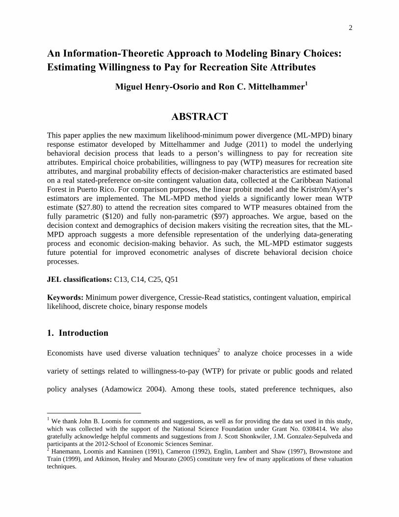
This paper applies the new maximum likelihood-minimum power divergence (ML-MPD) binary response estimator developed by Mittelhammer and Judge (2011) to model the underlying behavioral decision process that leads to a person’s willingness to pay for recreation site attributes. Empirical choice probabilities, willingness to pay (WTP) measures for recreation site attributes, and marginal probability effects of decision-maker characteristics are estimated based on a real stated-preference on-site contingent valuation data, collected at the Caribbean National Forest in Puerto Rico. For comparison purposes, the linear probit model and the Kriström/Ayer’s estimators are implemented. The ML-MPD method yields a significantly lower mean WTP estimate ($27.80) to attend the recreation sites compared to WTP measures obtained from the fully parametric ($120) and fully non-parametric ($97) approaches. We argue, based on the decision context and demographics of decision makers visiting the recreation sites, that the ML-MPD approach suggests a more defensible representation of the underlying data-generating process and economic decision-making behavior. As such, the ML-MPD estimator suggests future potential for improved econometric analyses of discrete behavioral decision choice processes. JEL classifications: C13, C14, C25, Q51 Keywords: Minimum power divergence, Cressie-Read statistics, contingent valuation, empirical likelihood, discrete choice, binary response models
1. Introduction
Economists have used diverse valuation techniques2 to analyze choice processes in a wide
variety of settings related to willingness-to-pay (WTP) for private or public goods and related
policy analyses (Adamowicz 2004). Among these tools, stated preference techniques, also
1 We thank John B. Loomis for comments and suggestions, as well as for providing the data set used in this study, which was collected with the support of the National Science Foundation under Grant No. 0308414. We also gratefully acknowledge helpful comments and suggestions from J. Scott Shonkwiler, J.M. Gonzalez-Sepulveda and participants at the 2012-School of Economic Sciences Seminar. 2 Hanemann, Loomis and Kanninen (1991), Cameron (1992), Englin, Lambert and Shaw (1997), Brownstone and Train (1999), and Atkinson, Healey and Mourato (2005) constitute very few of many applications of these valuation techniques.
3
known as direct or contingent valuation (CV) methods, stand out because of their frequent
application and complexity compared with revealed preference methods (Adamowicz and
Deshazo 2006).3
Behavioral models have become the dominant framework in the theoretical and empirical
choice literature for understanding the underlying decision processes that lead to a person’s
WTP. These models are also useful for estimating welfare measures based on stated preference
data. As Louviere, Hensher and Swait (2000) point out, these choice models and their underlying
assumptions, stemming from McFadden’s seminal work on random utility maximization theory,
form the theoretical context for discrete choice models, including binary response models
(BRMs).
Since the late 1980s, the large majority of practitioners who have applied discrete choice
models empirically have chosen parametric statistical procedures on the basis of precedent and
readily available softwares. Typical methods of analysis require a full parametric functional
specification of the relationship between the regressors and the response variable, and more
importantly, a full specification of a parametric distribution of the disturbances (e.g., the probit
(normal) or logit cumulative distribution functions [CDFs]). Although some distributional
assumptions can be benign, especially if the parameterization is flexible enough to describe
behavior adequately (McFadden 1994; McFadden and Train 2000), the implementation of an
incorrect parametric functional form can lead to spurious statistical inferences due to biased and
inconsistent estimates. Moreover, underlying economic theory provides little guidance for these
functional specifications, so there is insufficient information regarding the appropriate
distribution to adopt in practice (Mittelhammer, Judge and Miller 2000; Crooker and Herriges
3 For a more comprehensive review of the CV instrument, see Hausman (1993), Diamond and Hausman (1994), Hanemann (1994), and Venkatachalam (2004).
4
2004). Thus, any (parametric) functional specification for either the stochastic error or the utility
differences used in these methods is in general uncertain and questionable (Creel and Loomis
1997).
This study applies the new ML-MPD binary response estimator, developed by Mittelhammer
and Judge (2011), in which the parametric functional form of the conditional expectation as well
as the parametric family of probability distributions underlying binary responses are not
specified a priori. The ML-MPD estimator begins in a nonparametric context regarding model
specification. Then, information theoretic methods are applied to orthogonality relationships in
the form of sample moments that lead to a parametric family of probability distributions, a
conditional expectation function for the BRM, and estimators for the unknowns of the model.
Unlike most nonparametric methods, the ML-MPD does not employ the usual kernel density
estimation methodology with the attendant implementation choices relating to bandwidth, kernel
function, and other tuning issues. The ML-MPD approach effectively avoids using model
specification information that the econometrician generally does not really have, and thereby
reduces the potential for specification errors. The ML-MPD estimator is ultimately based on a
large varied family of CDFs, relies only on a minimal set of orthogonality conditions, and is free
of user specified tuning parameters.
Several distribution-free estimators for estimating BRMs have already been proposed in the
literature to overcome model misspecification issues (e.g., Manski 1975; Turnbull 1976; Cosslett
1983; Horowitz 1992; Matzkin 1992; Klein and Spady 1993; Li 1996; Chen and Randall 1997;
Creel and Loomis 1997; Huang, Nychka and Smith 2008). However, none of these estimators
have found widespread application in the empirical discrete choice literature for a number of
reasons that may include: 1) users’ lack of understanding regarding the estimation and inference
5
gains of the approach in empirical applications; 2) difficulty in interpreting results of the
analysis; 3) nonidentification of model parameters (e.g., the Klein and Spady (1993) estimator4
[KS]); and 4) ambiguity and/or uncertainty regarding the appropriate choices for tuning
parameters and other estimator implementation-computational issues.
Creel and Loomis (1997) underscore that the required scale and local normalizations for the
identification of KS parameter estimates are questionable because they go beyond restrictions
implied by demand theory. Moreover, it has been found that other suggested semiparametric
methods do not achieve root-n consistency (e.g., the Manski [1985] and Horowitz [1992]
estimators), and their finite sample behavior is in question (e.g., the Cosslett [1983], KS and
Ichimura [1993] estimators).5 And while fully non-parametric estimation techniques tend to be
more robust to incorrect functional specifications of conditional expectation functions as well as
probability distributions, they involve various choices of tuning parameters, kernels, and other
implementation choices. Sampling behavior in smaller-sized samples is also problematic.
Crooker and Herriges (2004) state that the gains and losses from using non-parametric and semi-
parametric estimators to recover WTP measures relative to the standard parametric approaches
are still unknown. There remains a continuing need to seek robust and efficient methods for
analyzing discrete choice behavior.
The empirical application in this paper relates to a stated-preference CV on-site dataset
collected at the Caribbean National Forest (CNF) in Puerto Rico (other researchers who have
used this data include Gonzalez, Loomis and Gonzalez-Caban (2008) and Santiago and Loomis
(2009)). In order to compare the new ML-MPD estimator to other leading methods for analyzing
BRMs, we implemented two prominent alternative estimation methods, including a fully
4 The KS estimator is considered a “best” semiparametric estimator because its asymptotic covariance matrix has been shown to achieve the semiparametric efficiency bound. 5 See Chen and Khan (2003) for more details.
6
parametric and a fully nonparametric estimator that have been employed in the CV literature, in
particular, the linear index probit model and the Kriström (1990)/Ayer et al. (1955) approach.
In the next section, we describe and characterize the dataset utilized in this study. Section 3
presents the implementation of the ML-MPD estimator in detail. In section 4, we discuss the
estimation results, and we provide concluding remarks in section 5.
2. Data
The dataset is comprised of 718 in-person interviews acquired at ten different recreation sites
along the Mameyes and Espiritu Santo rivers at the CNF in Puerto Rico during the summers of
2004 and 2005. The data was collected through dichotomous-response CV surveys, employing
the single-bounded6 bidding approach as the elicitation protocol, which is also referred to in the
literature as the “closed-ended” CV approach or the “take-it-or-leave-it” approach. Additional
details of the survey and its design are given in Gonzalez-Sepulveda (2008).
The survey asked each recreation user the following CV question: “Taking into consideration
that there are other rivers as well as beaches nearby where you could go visit, if the cost of this
visit to this river was $____more than what you have already spent, would you still have come
today?___Yes___No”. The hypothetical cost of the visit was randomly drawn from a pool of 18
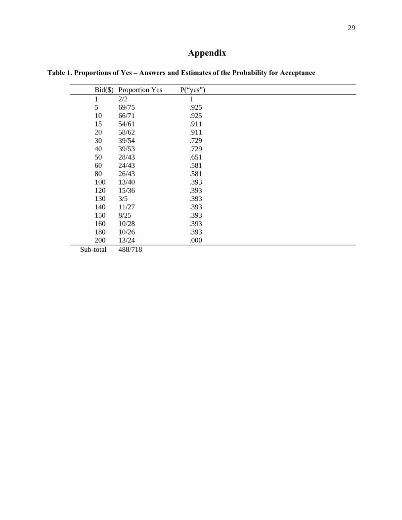
bid thresholds for each respondent, and ranged from $1 to $200 (see Table 1). Information on
site attributes (road quality, volume and speed of water in the pools, and size of rocks around the
pools), the recreation user’s income, and trip information (travel cost and travel time) were also
collected. Previous work demonstrated that when including trip information in the models, the
signs of the estimated coefficients for “travel cost” and “travel time” were not consistent with
6 This approach has the potential to be less efficient than the double-bounded protocol, however, McFadden (1994) and Cooper, Hanemann and Signorello (2001) have documented that the single-bounded CV question eliminates the response inconsistency and its associated bias.

7
theoretical expectations. By including travel time information as an indicator (= 1 if the travel
time to the CNF is more than 30 minutes and equal to 0 otherwise), as Cameron and James
(1987) propose, we obtain theoretically consistent results. Tables 2 and 3 summarize the
variables included in the estimated model, along with selected descriptive statistics.
The socio-demographic information in Table 3, indicate that lower income, moderately
educated, middle-aged male visitors dominated the sample outcomes.
3. Model and Estimation Framework
We present the ML-MPD estimation procedure in this section. The linear probit model and the
nonparametric7 estimators are well documented in the literature and are not reviewed here. All of
the statistical approaches used in this study allow one to model the underlying decision-makers’
choices made from a single, finite and exhaustive choice set with mutually exclusive alternatives.
We calculated a compensated WTP measure as an aggregate net estimate of WTP for the probit
ML and ML-MPD models based on a grand constant term (see Hanemann, 1984, 1989).
Regarding the Kriström/Ayer’s approach, we estimated the mean WTP through numerical
integration of the estimated survivor function (i.e., WTP probability distribution), excluding the
possibility of negative bids. The median WTP, in turn, is derived by finding the amount whose
acceptance probability equals 0.5.
This study makes the usual assumption that the observable discrete responses are the
outcomes of utility-maximizing choices made by decision-makers. The behavioral decision
process is assumed to be based on a linear and additive utility index, . * *i iY x β εi , also known
7 Boman, Bosted and Kriström (1999) show how Kriström/Ayer’s approach can be reinterpreted as an approximation of Dupuit’s consumer surplus. This describes what consumers would be willing to pay for obtaining some units of a good.

8
as a latent index model or a discrete choice behavioral-Random Utility Maximization model, so
that recreators choose the alternative that generates the greatest indirect utility.
3.1 Minimum Power Divergence Distributions
To motivate the ML-MPD estimator, note that the n -dimensional vector of unknown Bernoulli
probabilities corresponding to the BRM,
. * .1 | 1 , 1,..., x β x βi i i i iP y x p F F i n , (1)
is associated with an unknown link or transformation function F of factors affecting the
decision environment and that in practice is expressed in terms of an index function8 that is often
linear. However, more generally, one can always characterize the Bernoulli random variables
T n1 2, ,..., nY Y Y as being defined by ,i i iY p i , with zero-mean error, 0iE .
Without knowledge of the particular distributional specification of the link function, the
traditional ML approach is not available. One might then consider a Quasi-ML approach, but this
method does not assure the full set of attractive ML sampling properties (Mittelhammer, Judge
and Miller 2000), and moreover, it is difficult to characterize the actual sampling properties in
any given application. Alternatively, one might consider the two-stage Generalized Method of
Moment (GMM) estimator; however, the approach is not appealing for the current application
due to the ill-posed, underdetermined nature of the estimating equations of the problem (see
equation (2) ahead).
We pursue an empirical likelihood type estimator of β instead. Unlike classical estimation
procedures, these estimators rely on Kullback’s (1959) information theoretic minimum
8 This index is usually a function of the covariates xand a vector of β unknown parameters, which is estimated
along with the link function. Although non-linear specifications and the linear Box-Cox utility function are also
possible, the commonly used linear index representation . 0 1x xβi , with 1β being a vector of parameters, is
considered in this study.
9
discrimination information principle9 as well as on data-moment constraints, as defined in
Mittelhammer and Judge (2011). The basic estimation principle is to jointly estimate the
unknown parameters of the model along with the empirical sampling distributions that exhibit
minimum discrepancy relative to a reference distribution. The ML-MPD approach is robust in
terms of the uncountably infinite number of candidate distributions (such as symmetric, skewed,
uniform) that are members of the distribution class. It also maintains the full set of familiar ML
estimation and inference sampling behavior under familiar regularity conditions, and has been
shown to be potentially mean square error (MSE) superior to probit and logit estimators.
Moreover, the ML-MPD approach has been shown to be MSE superior to the best
semiparametric (KS) estimator under certain sampling conditions. All of the aforementioned
properties make this estimation procedure an appealing alternative relative to currently known
parametric and semiparametric alternative estimating procedures.
The application of the ML-MPD procedure can be conceptualized in two stages, although
implementation of the estimation methodology can be performed in one computational step. One
begins with an ill-posed inverse problem consisting of the nonparametric moment model
i i iY p ε noted above, along with generally applicable orthogonality conditions between
explanatory variables and model noise of the general form '( )E 0g X Y p . A minimum
power divergence solution for the probabilities is found that identifies a complete set of
probability distributions (i.e., the MPD solution) for the BRM. In a second stage, based on the
MPD class of probability distributions, ML estimation is used to estimate the unknowns that
9 An alternative to this principle is the maximum entropy principle, also known as the Shannon’s (1948) entropy measure or the generalized maximum entropy approach. Although there are some recent theoretical and empirical contributions in the econometric literature using the latter approach (e.g., Golan, Judge and Perloff, 1996; Crooker and Herriges, 2004; Marsh and Mittelhammer, 2004) a user of the method is also confronted with a notable number of “tuning parameter” type of decisions to make, for which the performance consequences are not well known currently.

10
occur in the class of probability distributions. The results of ML estimation produce estimates of
the effects of explanatory variables on the conditional Bernoulli probabilities, and also identify a
link function for those probabilities. In effect, the method estimates the form of the probability
model along with estimates of the unknowns in the model.
Regarding the first stage of the method, the Cressie-Read (CR)10 power-divergence family of
statistics (see Read and Cressie 1988; Imbens, Spady and Johnson 1998) measures the
discrepancy between probabilities to be estimated and a reference distribution for those
probabilities. Including sample moment constraints based on zero-mean theoretical population
conditions, the minimum power divergence extremum problem is specified as:
1
1, , 1,...,
Min CR , ,
s.t. '( )
0
pp q
g x y p 0
ip i i n
n (2)
where CR , ,p q is a member of the CR family, T
1 21
, ,..., 0,1n
ni
q q q
q is an n -
dimensional vector of reference Bernoulli probabilities, and , is the scalar power
parameter of the divergence measure. The sample moment constraint vector equation
1 '( )n 0g x y p
is of dimension 1m where : k mg is a real-valued measurable
function. The inequality constraints on the probability values are non-negativity constraints and
10 This goodness-of-fit measure contains the empirical likelihood statistic as a special case when 0 and
encompasses in its basic form the maximum entropy, the Kullback-Leibler statistic 1 and the Pearson’s2 statistic 1 , among others. As ranges from to the CR divergence measure leads to different
information theoretic estimators (see Mittelhammer, Judge and Miller 2000, Chapter 13.4; Lee, Chao and Judge 2010).
11
T
1 21
, ,..., 0,1n
ni
p p p p
represents an n -dimensional vector of updated conditional-on-x
Bernoulli probabilities (estimated empirical/sample distribution) underlying the binary decisions.
Mittelhammer et al. (2004) point out that some potential candidates for specifying g x are
the n k matrix x of explanatory variables as well as powers and cross products of the same
matrix. If one or more explanatory variables are determined simultaneously with the dependent
variable or some regressors are statistically dependent with the unobservable stochastic noise
component (i.e.
1 ' 0 x εE n ), then instrumental variables whose elements are uncorrelated
with the noise component but correlated with the endogenous entries in x should be included in
the specification of the orthogonality conditions (Mittelhammer and Judge 2009). In the current
application, the explanatory variables are exogenous and the function xg x was utilized.
The estimation objective function in (2) relies on the information theoretic CR power-
divergence criterion, which in the binary case takes the following form (Mittelhammer and Judge
2011):
1
11 1 1
1
1CR , ,
p q
ni i
i ii i i
p pp p
q q (3)
The discrepancy measure is always positive valued unless i ip q , no matter the choice of ,
becomes larger the more divergent are ip and iq , is convex in the 'ip s , and is second order
continuously differentiable. On the basis of the constrained minimization problem specified in
(2) and (3), the MPD family of CDFs solution for this extremum problem is given by:
12
1; , arg when < 0
1
arg when = 0 1
1
0
0i
i i
i ii
i i
p
i ii
i i
i p
p pp w q w
q q
p pLn Ln w
q q
1
1 1
1
(4)
1
1 arg when 0 and 1 ,
1
10
0
i
i i
i i i ii
i i
i
p
qp p
w w q qq q
q
where . x λi iw , and represents the 1m vector of Lagrange multipliers of the moment
constraints when the problem is expressed in Lagrange form. The definition in (4) characterizes
an uncountably infinite number of distributions, with argument iw , indexed by the values of
and iq . For example, when 0 and 0.5iq , the standard logit model is subsumed by the
family of distributions. It is clear that the inverse cumulative distribution function of the MPD
family always exists in closed form, but except for a measure zero set of possibilities for
and iq , the probabilities themselves must be solved for numerically. Fortunately, strict
monotonicity properties of the terms involving the 'ip s in (4) make for a relatively
straightforward numerical solution procedure that is guaranteed to solve for the appropriate ip
for any admissible argument, iw , of the CDF. Further discussion of the MPD family of
distributions, including their myriad different shapes and characteristics, can be found in
Mittelhammer and Judge (2011).
13
3.2 The ML-MPD estimator
The family of probability distributions in (4) was used as a basis for specifying the likelihood
function associated with the data outcomes in the usual way, leading to a log-likelihood function
of the general form . .1
; , ; ,1, , ln 1 ln
x xqi i
n
i i i ii
p q p qL y y , where we
define .11 In the implementation of the distribution family, we specify iq q i , which is
tantamount to assuming that the same basic probability distributional form is used across the
observations in forming the conditional Bernoulli probabilities. In this context, it is the 'i sx , and
thus the arguments of the distributions, that change the probabilities across decisions makers.
The likelihood function was maximized using the non-gradient based Nelder-Mead simplex
minimization algorithm proposed by Nelder and Mead (1965) (the negative of the likelihood
function was minimized to obtain the maximum).12 This optimization method belongs to the
general class of “direct search methods” and has become one of the most widely used techniques
for non-linear unconstrained optimization. It does not rely on gradients or Hessians, so it tends to
be faster between iterations than search methods that depend on derivatives of the objective
function (e.g., Newton-Raphson). The Nelder-Mead approach is also immune to numerical
problems caused by highly nonlinear and sometimes unstable gradient and/or Hessian
calculations from iteration to iteration.
In order to promote both stability and accuracy in the search for the ML optimimum, while
guarding against converging to local optima, we first implemented a recursive grid search
approach in the direction with increments of 0.2 . In particular, we set the global values of
11 A formal argument of equating the Lagrange multiplier vector λ and the unknown parameter vector β is given in
Judge and Mittelhammer (2012), Chapter 10. 12 A detailed explanation of this algorithm and its implementation can be found in Nelder and Mead (1965) and Jacoby, Kowalik and Pizzo (1972).
14
external to the rest of the optimization problem, and sequentially updated the starting values
based on the lagged recursive solutions for the previous value of , beginning with the standard
logit solution ( 0, .5q in the MPD family of distributions). The recursive method does not
guarantee a global optimum but reduces the possibility of not searching in the neighborhood of
the global optimum. We also embedded a search for the optimal q along the grid from 0.01 to
0.99, in .01 increments. The likelihood function was ultimately maximized at the values
*ˆ 4.4 and *ˆ .88q (see section 4.3).
Upon identifying the ML solution, the variance-covariance matrix of β was estimated by
substituting the optimized ML estimates *̂ and *q̂ , and the optimized ML-MPD parameter
estimates *β̂ into the definition of the MPD distribution in (4) 13. The resulting expression is the
value of a profile likelihood function for the parameter vector , which can be used to calculate
the asymptotic covariance matrix of the ML estimates, and for conducting inference. Since ip is
implicit in (4), the variance-covariance matrix is derived using implicit differentiation and the
'ip s are solve for numerically. The variance-covariance matrix was estimated using the “outer-
product-of-gradients” approach, based on the computation of the inverse of
L L
,
where
L
is the n k matrix of derivatives of the log of the profile likelihood function
contributions, , 1,...,iL i n with respect to β .
For implementing all of the preceding procedures relating to the MPD estimator, as well as
the implementation of the probit maximum likelihood estimator (MLE), we used Aptech
13 Notice that if the optimized gamma is > 0, the resulting MPD CDF will be a model with finite bounded support, whereas for < 0, as is the case here, the MPD CDF has infinite support in both the positive and negative directions.

15
Systems’ GAUSSTM 11. The Kriström/Ayer estimator was implemented using the software
environment for statistical computing and graphics R (R Development Core Team 2009).
4. Results and discussion
All of the models discussed in this section utilize the seven explanatory factors that are defined
in Table 2.
4.1 Parametric Model Results
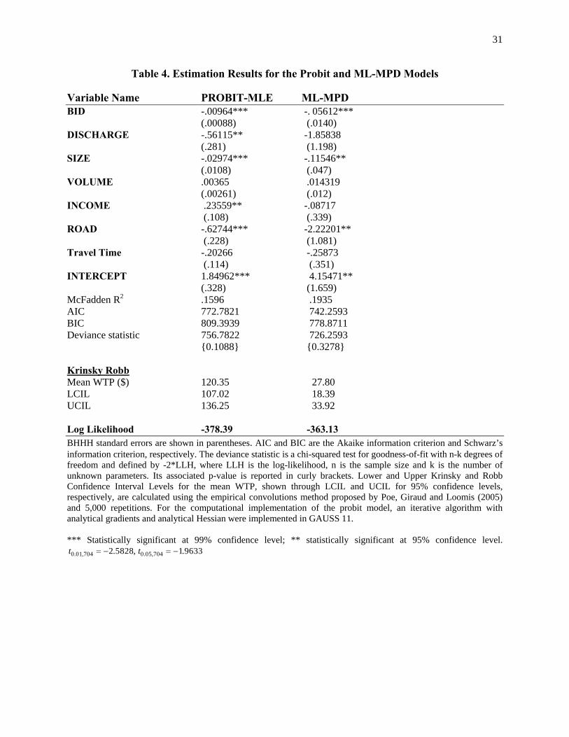
Using the conventional parametric structure of the probit model, we adopted the Berndt-Hall-
Hall-Hausman (BHHH) estimator (Berndt et al. 1974) to find the maximum likelihood estimator
of the linear probit model, and the results are displayed in Table 4. The “bid” variable is highly
significant and its sign is aligned with economic theory, indicating that the higher the visit price
to the park, the less willing respondents are to pay. According to the CV literature (see e.g.
Hanemann 1984; Haab and McConnell 2002; Gonzalez, Loomis and Gonzalez-Caban 2008),
income has typically, but not necessarily, been dropped in these types of studies due mainly to
the lack of statistical significance. However, based on the dichotomous indicator, the "income"
variable was found to be significantly different from zero in the parametric approach. The
variables “bid”, “size” (size of the rocks around the pool) and “road” (non-paved roads)
contribute to the explanation of the dependent variable at the 0.01 level of type I error. “Income”
and “volume” are both positively related to the probability of paying the bid amount, whereas the
variables “discharge”, “road”, “size” and “non-residents” are negatively associated.
Table 4 also reports the mean economic value of a visit to the rivers at the CNF as well as its
corresponding confidence intervals (CIs). Employing the parametric and non-symmetric CI
16
Krinsky and Robb (1986)14 simulation method for the mean WTP and Hanneman's approach for
estimating the mean WTP (see section 3), the mean WTP measure is $120 and the 95% CI
ranges from $107 to $136.25. We note that either of these levels of WTP for the types of
recreators surveyed, as well as the type of recreation experience obtained by a visit to the
Caribbean National Forest, appears to be unrealistically high.
4.2 Nonparametric Model Results
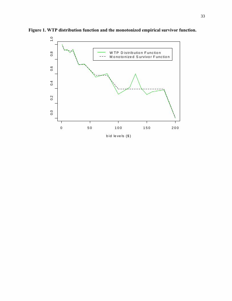
Relating to the non-parametric estimation approach, Figure 1 illustrates both the proportion of
individual WTPs for each ordered bid class (a so-called empirical survivor function or Ayer
function) and the monotonized empirical survivor function F(p) using the non-parametric
technique.15 Both curves were derived by setting the probability of a “yes” response equal to one
at $0 and the maximum bid amount as the truncation upper limit point (T = $200 ; see
frequencies of “yes” responses for each bid level and the distribution-free Maximum Likelihood
estimates of the probability for acceptance in Table 1). The monotonized function represents a
set of ML estimates (or maximizing set) of desired probabilities, which provides a continuous
linear smoothed function with a non-constant slope. In the context of the current study, each ML
estimate symbolizes the survival probability of WTP given a specific bid level. As the sample
size becomes infinite, the estimated proportions will converge in probability to the true
14 Under this simulation procedure, draws of coefficient estimates are taken from their asymptotic distribution (i.e.,
ˆ ~ ,VCOV , 5,000 r N r ), after calculating the Cholesky decomposition (p) of the VCOV matrix,
calculating a vector of parameter estimates such that 'ˆ ˆ ˆ* r p , and computing the WTP of interest. Park,
Loomis, and Creel (1991) constitute an application of this simulation technique in CV studies. 15 This distribution-free estimator has desirable ML properties, represents a closed-form solution to the Non-Parametric ML problem for single-bounded discrete choice data, and yields a monotonically non-increasing sequence of likelihoods of accepting the bid (i.e., , p bidF p P WTP bid ). If the sequence is not monotonic
in some regions for some bids, then the pool-adjacent-violators (PAVA) algorithm is applied. This smoothing procedure is repeated until a monotonic sequence of aggregated proportions emerges at each bid level. For more details on this technique, see Robertson, Wright and Dykstra (1988).
17
probability of success and the new sequence will provide a distribution-free nonparametric
maximum likelihood estimator of the probability of success (Ayer et al. 1955).
Several findings can be derived from Figure 1. First, to obtain the monotonic survivor
function, constraining WTP to be non-negative upon assuming that 1 and 0 when the bid is
$0 and $200, respectively, appears to be a reasonable approximation of behavior between the
known points (“bids”). That is, if the bid is zero, then the probability of accepting the payment is
unity and if the price is $200 the probability is zero since it is understood to be too high and,
therefore, no one will be willing to accept the offered price. Second, the plot indicates that as the
bid increases, the probability of WTP decreases.
Although the selection of the truncation point is an empirical problem in the non-parametric
literature (see Duffield and Patterson 1991) and its sensitivity must be noted, we integrated the
smoothed survivor function up to the maximum bid level to obtain the mean WTP, following the
approach of Creel and Loomis (1997). Using numerical integration
200
01
TE WTP F p dp and bootstrap pair resampling, the unconditional truncated
mean compensated variation (WTP) is $97 and the 95% bootstrap CI ranges from $66.5 to $124.
Note that the mean fully nonparametric WTP estimate does not fall within the 95% confidence
interval for the mean WTP ($107, $136.25), constructed for the fully parametric estimator, and
that while the level of mean WTP is lower than that of the parametric approach, the
nonparametric WTP value still seems unrealistically high for the types of recreators surveyed
and the type of recreation experience obtained.
18
4.3 ML-MPD Model Results
The value of the ML estimate, ˆβML MPD , of the vector corresponding to the ML estimates of
*ˆ 4.4 and *ˆ .88q , is presented in Table 4. Substituting these point estimates into the MPD
definition in (4) for 0 yields the estimated WTP probability distribution:
4.4 4.4
* *. .
1ˆˆ; , arg 4.4
0.88 1 0.88
x x 0i p i
p pp w q w (5)
where . .ˆ
x x βi i ML MPDw , and .ix denotes a 1 k row vector contained within the n k matrix x
of covariates, or any other vector value of interest relating to the explanatory variables.
There is no closed form solution for the probabilities in (5). Accordingly, the derivatives of
* *ˆˆ; ,p w q with respect to β needed to form the asymptotics covariance matrix are derived via
implicit differentiation. The resulting n k matrix of derivatives is given by
4.4 5.45.4 4.4
1
0.88 1 (1 0.88)
p xβ p p
(6)
where denotes the Hadamard (elementwise) product operator, all the division operations are
Hadamard (elementwise) division, and p is the 1n vector of estimated probabilities. As
indicated in section 3, the outer product of the gradient method is then used to define the k k
variance covariance matrix as
L L
1
β β
β β.
The empirical probabilities in (5) were recovered numerically using the interval bisection
method. Interested readers are referred to Mittelhammer and Judge (2011) for additional detail
on the computational methodology. Table 4 summarizes estimated coefficients and their
19
corresponding asymptotic standard errors as well as willingness to pay results for the MPD-ML
estimator.
A number of interesting findings can be deduced from the results reported in Table 4. First of
all, based on the goodness-of-fit measures reported (pseudo R2, AIC, BIC, and deviance
statistics) the ML-MPD model performs better than the probit model despite the fact that both
models do not exhibit misspecification problems according to the outcome of the deviance
goodness-of-fit test. Second, the parameter estimates in these two models have the same signs,
except for the "income" variable. As mentioned previously, this dichotomous income indicator is
positively related to the probability of paying the bid amount based on the probit model, but
when using the ML-MPD approach, a negative effect of income is estimated, although the effect
is not statistically significant. Third, there are sizeable differences in the magnitudes of the
coefficients, where most of the ML-MPD estimates tend to be larger compared to the probit point
estimates, although this by itself is not remarkable, given the notably different probability
distribution functions for which the explanatory factors are arguments. Fourth, the MPD
approach does not produce uniformly smaller estimated standard errors relative to probit. Under
the fully parametric model the variables that are statistically significantly at the .01 level are the
“bid”, "size", and “road” regressors. However, under the ML-MPD approach, only “bid” is
significant at that level, although “size” and “road” are significant at the .05 level. The outcome
of having just "bid" statistically significant at the .01 level is consistent with Gonzalez-Sepulveda
(2008)'s findings. The "discharge" variable is insignificant at conventional levels in the ML-
MPD case, but is nearly significant at the 0.10 level, suggesting its effect should not necessarily
be ignored.

20
4.4 Comparison of Marginal Effects and WTPs
Using the estimating parameters derived from the probit and ML-MPD models, marginal
effects16 of changes in the explanatory variables on mean WTP were calculated from Table 4. It
should be mentioned that marginal effects from the Kriström (1990)/Ayer et al. (1955) approach
were not computed, considering the fact that the essence of this empirical method consists only
to serve as a mean or median WTP estimation technique given by the area under the empirical
survivor function.
Based on the probit results, visitors were willing to pay -$58 and -$65 for increasing in-
stream flows and non-paved roads, respectively, as well as -$3 for increasing size of rocks or
sand around the pools. This indicates that increased stream flows, non-paved roads, and larger
rock/sand sizes provide disutility to recreation users. The volume of water in the pools positively
influences the WTP of recreation users, being the marginal effect $0.37. These marginal effects
on WTP across site attributes become larger when employing the ML-MPD approach. For
instance, visitors are willing to pay -$33 and -$40 for increasing in-stream flows and non-paved
roads, respectively. The amount relating to the size of rocks or sand becomes -$2, whereas the
marginal effect associated to the volume of water in the pools is $0.25.
We also calculated marginal effects on the mean probabilities of acceptance of bids as a
function of one unit changes in the levels of explanatory factors from the probit and ML-MPD
16 Marginal effect values are obtained for the probit and ML-MPD cases using the mean marginal effect approach. In the estimation procedure, there is potentially a different marginal effect at every observation if the observations evaluate different probabilities. For the probit model, the marginal effect representation is given by
1.ˆ ˆ , i=1,...,n, j=2,...,k and x βi ji
n is the standard Normal probability density function, while in the case of
ML-MPD the marginal effects are represented by
ˆ ˆ* *ˆ ˆ* 1 * 1
1
* *
ˆ
ˆ ˆ1 1
ML MPD j
i
i i
np q p q
for 0 , where
j=2,...,k, * * ˆˆ ˆ, q , and ML MPD are the optimized ML point estimates reported above, pi are the empirical probabilities,
and i=1,...,n.
21
models (see Table 5). These marginal effect outcomes were not calculated for the fully
nonparametric approach, following the same argument previously mentioned. It is evident from
table 5 that the effects on probabilities of one-unit changes in explanatory variables is notably
different in magnitude for the probit and ML-MPD approaches, albeit except for income, the
directional effects are the same. For income, the mean marginal effects contrast both in sign and
magnitude. The impact of a one-unit change in travel time (i.e., indicating that travel time to the
CNF takes over 30 minutes) is -0.06 for probit and -0.02 for ML-MPD. For every additional
millimeter of grain size, the probability of bid acceptance decreases by 0.088 and 0.070 for the
probit and ML-MPD methods, respectively. The probability of visiting recreational sites
decreases substantially for non-paved roads and for increased water discharge based on both
estimation approaches, although relatively speaking, the effects for the probit model, -.1662 and
-.1858 respectively, are much higher than for the ML-MPD approach, being -.1125 and -.1345.
As for mean WTP for a visit to the CNF, the ML-MPD WTP of $27.80 is substantially lower
than the results of the probit ($120) and nonparametric ($97.00) approaches, respectively. We
note that a 95% CI under ML-MPD as well as the mean WTP measure were computed in a
similar manner, as we described previously in section 4.1. It is apparent from the fact that the
CI’s are non-overlapping that the mean WTPs are estimated to be statistically different via the
two approaches (this is true at any typical level of confidence (including 99%). To formally test
whether there is a difference in WTP distributions for the probit and ML-MPD (i.e. Ho: WTPprobit
= WTPML-MPD), we implemented the nonparametric complete combinatorial convolution
approach of Poe, Giraud and Loomis (2005). A two-tailed p-value equal to 0.00082 rejects the
null hypothesis convincingly, and it can be concluded that the two empirical WTP distributions
are statistically different. In terms of providing information on mean WTP, the ML-MPD is more

22
informative and precise than the probit and fully nonparametric approach. For a 95% nominal
coverage, the average CI length for the ML-MPD approach is $15.53, whereas for probit and
Kriström/Ayer’s estimators this interval is wider at $29.23 and $57.52, respectively.
5. Implications and Conclusions
A major finding of this study is that the ML-MPD approach yields a substantially lower
estimate of the mean WTP ($27.80) for visiting the recreation sites compared to WTPs obtained
from the fully parametric ($120) and fully non-parametric approaches ($97). We argue, based on
the decision context and demographics of decision makers, that the lower WTP value is a much
more reasonable and defensible estimate of the WTP for visiting the recreation sites. Gonzalez-
Sepulveda (2008; Chapter three), using the same dataset and compensated WTP measures, but
only a smaller subsample of the data, arrived at a related insight with regard to the level of WTP
when comparing the Travel Cost Model (TCM) with the parametric logit model (CV method).
Sampling issues affecting TCM and CV estimates are potentially part of the explanation for the
difference in the WTP estimates obtained from these two approaches, including spatial
truncation of TCM recreation markets and endogenous stratification of CV respondents in the
sample. Estimates from the ML-MPD approach suggest yet another reason for the difference in
WTP values -- relaxing the rigid distributional assumptions of the conventional parametric
methods produce substantially lower WTP estimates.
Another implication worthy of note is that income, expressed in terms of an income indicator
of a $20,000 threshold, was statistically significant under the parametric approach, but
insignificant, and nominally estimated to have a negative effect, based on the ML-MPD
methodology. Income effects are often disregarded in CV studies, mainly due to insignificance
23
of the model parameter. Carson and Hanemann (2005) identify several sources of measurement
errors that have contributed to biasing estimated income effects downward. While treating the
effect of income as an indicator variable is not a common practice in CV, Aiew, Nayga and
Woodward (2004) recognized how attractive an exploration of this type of specification might
be, especially when understanding that the WTP distribution across income groups might be
important from a policy perspective. Champ et al. (2002) conducted one of very few CV
published studies that included income as an indicator variable. A negative effect of an income
threshold over $20,000 is suggestive of wealthier Puerto Ricans not preferring visiting water
pools, but possibly preferring other types of recreation (e.g., boating to nearby islands, visiting
resorts ). While the negative effect is not statistically significant, the ML-MPD result seems more
plausible than the result obtained with the probit model, especially when considering that more
than half of the respondents who report that visiting the water pools was the main purpose of the
trip had an annual income of less than $15,000. The negative income effect is also consistent
with the mean ML-MPD WTP value of $27.80 compared to the substantially higher WTP values
obtained using the other two approaches, which appear patently unrealistic relative to the
demographics of the individuals who visit the water pools.
In contrast to many alternative estimators, the ML-MPD procedure is free of subjective
choices relating to various tuning parameters, has the flexibility to fit a wide range of varied
distributional shapes to conform to the choices observed, and proceeds by imposing minimal
assumptions on the information contained in the data. In addition, sampling experiments
conducted by Judge and Mittelhammer (2012) to investigate the small sample properties of a
range of MPD-based estimators and parametric methods (e.g. the probit model) indicate that the
former ones compare more favorably in terms of MSE relative to parametric methods.

24
As such, the new ML-MPD approach to estimation of BRMs appears to have potential for
providing a more defensible representation of the underlying data-generating process and
economic decision-making behavior, and improved econometric analyses of discrete choice
processes compared to the commonly used parametric methods.
25
References
Adamowicz,W.L. 2004. What’s it worth? An Examination of historical trends and future directions in environmental valuation. The Australian Journal of Agricultural and Resource Economics. 48:3, pp. 419 – 443.
Adamowicz,W.L. and J.R. Deshazo. 2006. Frontiers in States Preference Methods: AN Introduction. Environmental & Resource Economics. 34: 1 - 6.
Aiew,W., Nayga,R.M. and R.T.Woodward. 2004. The treatment of income variable in willingness to pay studies. Applied Economics Letters. 11: 581 - 585.
Atkinson,G., Healey,A. and S.Mourato. 2005. Valuing the costs of violent crime: a stated preference approach. Oxford Economic. Paper 57, 559 – 585.
Ayer,M., Brunk,H.D., Ewing,G.M., Reid,W.D. and E.Silverman. 1955. An Empirical Distribution for sampling with Incomplete Information. The Annals of Mathematical Statistics, Vol. 26, No.4, December, pp. 641 – 647.
Berndt,E.K., Hall,B.H., Hall,R.E. and J.A.Hausman. 1974. Estimation and inference in nonlinear structural models. Annals of Economic and Social Measurement. 3(4): 653 – 665.
Boman,M., Bosted,G. and B. Kriström,B. 1999. Obtaining Welfare Bounds in Discrete-Response Valuation Studies: A Non-Pametric Approach. Land Economics. 75(2): 284 – 294.
Brownstone,D. and K.Train. 1999. Forecasting new product penetration with flexible substitution patterns. Journal of Econometrics. 89(1-2): 109 – 129.
Cameron,T.A. 1992. Combining Contingent Valuation and Travel Cost Data for Valuation of Non-market Goods. Land Economics. 68: 302 – 317.
Cameron,T.A. and M.D.James. 1987. Estimating Willingness to Pay from Survey Data: An Alternative Pre - Test – Market Evaluation Procedure. Journal of Marketing Research, Vol.24, No.4, November, pp 389 – 395.
Carson,R.T and W.M.Hanemann. 2005. Contingent Valuation. In: Handbook of Environmental Economics. Volume 2. Edited by K.G.Maler and J.R.Vincent.
Champ,P.A., Flores,N.E., Brown,T.C. and J.Chivers. 2002. Contingent Valuation and Incentives. Land Economics. 78(4): 591 - 604.
Chen,H.Z. and A.Randall. 1997. Semi-nonparametric estimation of binary response models with an application to natural resource valuation. Journal of Econometrics. 76(1-2): 323 – 340.
Chen,S. and S.Khan. 2003. Rates of convergence for estimating regression coefficients in heteroskedastic discrete response models. Journal of Econometrics. 117: 245 – 278.
Cooper,J.C., Hanemann,W.M. and G.Signorello. 2001. One-and-one-half-bound dichotomous choice contingent valuation. CUDARE working paper No. 921. University of California, Berkeley.
Cosslett,S. 1983. Distribution-Free Maximum Likelihood Estimation of the Binary Choice Model. Econometrica. 51: 765 – 782.
Creel,M. and J.Loomis. 1997. Semi-nonparametric Distribution-Free Dichotomous Choice Contingent Valuation. Journal of Environmental Economics and Management. 32: 341 – 358.
Diamond,P. and J.Hausman. 1994. Contingent Valuation: Is Some Number Better Than No Number? Journal of Economic Perspectives. 8(4): 45 – 64.
Duffield,J.W. and D.A.Patterson. 1991. Inference and Optimal Design for a Welfare Measure in Dichotomous Choice Contingent Valuation. Land Economics. 67(2): 225 – 239.
26
Crooker,J.R. and J.A.Herriges. 2004. Parametric and Semi-Nonparametric Estimation of Willingness-to-Pay in the Dichotomous Choice Contingent Valuation Framework. Environmental and Resource Economics. 27: 451 – 480.
Englin,J., Lambert,D. and W.D.Shaw. 1997. A Structural Equations Approach to Modeling Consumptive Recreation Demand. Journal of Environmental Economics and Management, 33: 33-43.
Golan,A., Judge,G. and J.Perloff. 1996. A Maximum Entropy Approach to Recovering Information from Multinomial Response Data. Journal of the American Statistical Association. 91: 841 – 853.
Gonzalez-Sepulveda,J.M. 2008. Challenges and Solutions in Combining RP and SP Data to Value Recreation. Doctoral Dissertation. Colorado State University. Department of Agricultural and Resource Economics.
Gonzalez,J.M., Loomis,J.B. and A.Gonzalez-Caban. 2008. A Joint Estimation Method to Combine Dichotomous Choice CVM Models with Count Data TCM Models Corrected for Truncation and Endogenous Stratification. Journal of Agricultural and Applied Economics. 40(2): 681 – 695.
Gonzalez-Sepulveda,J.M. and J.B.Loomis. 2010. Do CVM Welfare Estimates Suffer from On-Site Sampling Bias? A Comparison of On-Site and Household Visitor Surveys. Agricultural and Resource Economics Review. 39(3): 561 - 570.
Haab,T. and K.McConnell. 2002. Valuing environmental and natural resources: the econometrics of non-market valuation. Northampton, MA: Edward Elgar.
Hanemann,W.M. 1984. Welfare evaluations in Contingent valuation Experiments with Discrete Responses. American Journal of Agricultural Economics. 66(3): 332 – 341.
______________. 1994. Valuing the Environment Through Contingent Valuation. The Journal of Economic Perspectives. 8(4): 19 – 43.
Hanemann,M., Loomis,J. and B.Kanninen. 1991. Statistical Efficiency of Double-Bounded Dichotomous Choice Contingent Valuation. American Agricultural Economics Association. 1255 – 1263.
Hausman,J. 1993. Contingent Valuation: A Critical Assessment. North-Holland, New York. Horowitz,J.L. 1992. A Smoothed Maximum Score Estimator for the BRM. Econometrica. 60:
505 – 531. Huang,J., Nychka,D.W. and V.K.Smith. 2008. Semi-parametric discrete choice measures of
willingness to pay. Economics Letters. 101: 91 – 94. Ichimura,H. 1993. Semiparametric least squares (SLS) and weighted SLS estimation of single-
index-models. Journal of Econometrics. 58: 71 – 120. Imbens,G.W., Spady,R.H. and P.Johnson. 1998. Information Theoretic Approaches to Inference
in Moment Condition Models. Econometrica. 66(2): 333 – 357. Jacoby,S.L.S., Kowalik,J.S. and J.T.Pizzo. 1972. Iterative Methods for Nonlinear Optimization
Problems. Englewood Cliffs, NJ: Prentice Hall. Judge,G. and R.C.Mittelhammer. 2012. An Information Theoretic Approach to Econometrics.
Cambridge University Press, 248 pages. Klein,R.W. and R.H.Spady. 1993. An Efficient Semiparametric Estimator for Binary Response
Models. Econometrica. 61(2): 387 – 421. Krinsky,I. and A.Robb. 1986. On Approximating the Statistical Properties of Elasticities. Review
of Economics and Statistics. 68: 715 - 719.
27
Kriström,B. 1990. A Non-Parametric Approach to the Estimation of Welfare Measures in Discrete Response valuation Studies. Land Economics, Vol.66, No.2. pp. 135 – 139.
Kullback,S. 1959. Information Theory and Statistics. John Wiley and Sons. NY. Lee,J., Tan Chao,W.K. and G.G.Judge. 2010. Stigler’s approach to recovering the distribution of
first significant digits in natural data sets. Statistics and Probability Letters. 80(2): 82 – 88. Li,C. 1996. Semiparametric Estimation of the Binary Choice Model for Contingent Valuation.
Land Economics. 72 (4): 462 – 473. Louviere,J.J., Hensher,D.A. and J.D.Swait. 2000. Stated Choice Methods: Analysis and
Application. Cambridge University Press. Manski,C.F. 1975. The Maximum Score Estimation of the Stochastic Utility Model of Choice.
Journal of Econometrics. 3: 205 – 228. Marsh, T.L. and R.C.Mittelhammer. 2004. Generalized Maximum Entropy Estimation of a First
Order Spatial Autoregressive Model. Spatial and Spatiotemporal Econometrics. Advances in Econometrics, Volume 18, 199–234.
Matzkin,R. 1992. Non-Parametric and Distribution-Free Estimation of the Binary Threshold Crossing and the Binary Choice Models. Econometrica. 60: 239 – 270.
McFadden,D.. 1994. Contingent Valuation and Social Choice. American Journal Agricultural Economics. 76: 689 – 708.
McFadden,D. and K.Train. 2000. Mixed MNL Models for Discrete Response. Journal of Applied Econometrics. 15: 447 – 470.
Mittelhammer,R.C., Judge,G.G. and D.J.Miller. 2000. Econometric Foundations. Cambridge. Mittelhammer,R.C., Judge,G., Miller,D. and N.S.Cardell. 2004. Minimum Divergence Moment
Based Binary Response Models: Estimation and Inference. Working Paper. Mittelhammer,R.C. and G.G.Judge. 2009. Robust Moment Based Estimation and Inference: The
Generalized Cressie-Read Estimator. Statistical inference, econometric analysis and matrix algebra. Vol. IV. 163 – 177.
____________________________. 2011. A Family of Empirical Likelihood Functions and Estimators for the Binary Response Model. Journal of Econometrics. 164(2): 207 - 217.
Nelder,J.A. and R.Mead. 1965. A simplex method for function minimization. The Computer Journal. 7(4): 308 – 313.
Park, T., Loomis, J.B. and M.Creel. 1991. Confidence Intervals for Evaluating Benefits Estimates from Dichotomous Choice Contingent Valuation Studies. Land Economics. 67(1): 64 - 73.
Poe,G.L., Giraud,K.L. and J.B.Loomis. 2005. Computational Methods For Measuring The Difference of empirical Distributions. American Journal Agricultural Economics. 87(2): 353 - 365.
R Development Core Team (2009) R: A language and environment for statistical computing. R foundation for statistical computing. Vienna, Austria. http://www.R-project.org, ISBN 3-900051-07-0
Read,T.R. and N.A.Cressie. 1988. Goodness of Fit Statistics for Discrete Multivariate Data. Springer Verlag. NY.
Robertson,T., Wright,F. and R.Dykstra. 1988. Order Restricted Statistical Inference. New York: Wiley & Sons.
Santiago,L.E. and J.Loomis. 2009. Recreation benefits of natural area characteristics at the El Yunque National Forest. Journal of Environmental Planning and Management. 52(4): 535 – 547.

28
Shannon,C.E. 1948. A Mathematical Theory of Communication. Bell System Technical Journal. 27: 379 – 423.
Turnbull,B. 1976. The empirical distribution function with arbitrarily grouped, censored and truncated data. Journal of the Royal Statistical Society. Series B. 38: 290 – 295.
Venkatachalam,L. 2004. The contingent valuation method: a review. Environmental Impact Assessment Review. 24: 89 – 124.
29
Appendix
Table 1. Proportions of Yes – Answers and Estimates of the Probability for Acceptance
Bid($) Proportion Yes P(“yes”) 1 2/2 1 5 69/75 .925 10 66/71 .925 15 54/61 .911 20 58/62 .911 30 39/54 .729 40 39/53 .729 50 28/43 .651 60 24/43 .581 80 26/43 .581 100 13/40 .393 120 15/36 .393 130 3/5 .393 140 11/27 .393 150 8/25 .393 160 10/28 .393 180 10/26 .393 200 13/24 .000
Sub-total 488/718

30
Table 2. Variables Used in the Analyses
Variable Name Description
Choice = 1 if willing to pay the visit price = 0 otherwise
Bid Offered U.S. dollar amount (threshold) Road = 1 if non-paved road; = 0 otherwise Discharge Mean annual speed of water in the pool (cubic feet) Size Median grain size (millimeters) around the pools Volume Volume of the pool (cubic feet) Income = 1 if family annual income (U.S. dollars) is greater than $20,000
= 0 otherwise Travel Time = 1 if travel time (TT) exceed 30 minutes; = 0 otherwise Note: The variables volume, size, and income were scaled by 100, 10 and 1000, respectively, in estimation to support numerical stability and accuracy in calculations, and allow similar orders of magnitude for parameter estimates.
Table 3. Descriptive statistics for selected unscaled quantitative variables Variable Name Obs Mean Std.Dev. Minimum Maximum
Bid 718 63.53 58.27 1 200 Discharge 718 0.83 0.5711 0.11 1.67 Size 718 509.22 628.17 102 2337 Volume 718 446.74 414.00 42 1868.4 Income 718 28652 21893.50 5000 75000
Travel Time 718 63.52 59.62 1 990
31
Table 4. Estimation Results for the Probit and ML-MPD Models
Variable Name PROBIT-MLE ML-MPD BID -.00964*** -. 05612***
(.00088) (.0140) DISCHARGE -.56115** -1.85838
(.281) (1.198) SIZE -.02974*** -.11546**
(.0108) (.047) VOLUME .00365 .014319
(.00261) (.012) INCOME .23559** -.08717 (.108) (.339) ROAD -.62744*** -2.22201** (.228) (1.081) Travel Time -.20266 -.25873 (.114) (.351) INTERCEPT 1.84962 *** 4.15471** (.328) (1.659) McFadden R2 .1596 .1935 AIC 772.7821 742.2593 BIC 809.3939 778.8711 Deviance statistic 756.7822 726.2593 {0.1088} {0.3278} Krinsky Robb Mean WTP ($) 120.35 27.80 LCIL 107.02 18.39 UCIL 136.25 33.92 Log Likelihood -378.39 -363.13 BHHH standard errors are shown in parentheses. AIC and BIC are the Akaike information criterion and Schwarz’s information criterion, respectively. The deviance statistic is a chi-squared test for goodness-of-fit with n-k degrees of freedom and defined by -2*LLH, where LLH is the log-likelihood, n is the sample size and k is the number of unknown parameters. Its associated p-value is reported in curly brackets. Lower and Upper Krinsky and Robb Confidence Interval Levels for the mean WTP, shown through LCIL and UCIL for 95% confidence levels, respectively, are calculated using the empirical convolutions method proposed by Poe, Giraud and Loomis (2005) and 5,000 repetitions. For the computational implementation of the probit model, an iterative algorithm with analytical gradients and analytical Hessian were implemented in GAUSS 11. *** Statistically significant at 99% confidence level; ** statistically significant at 95% confidence level.
0.01,704 0.05,7042.5828, 1.9633t t
32
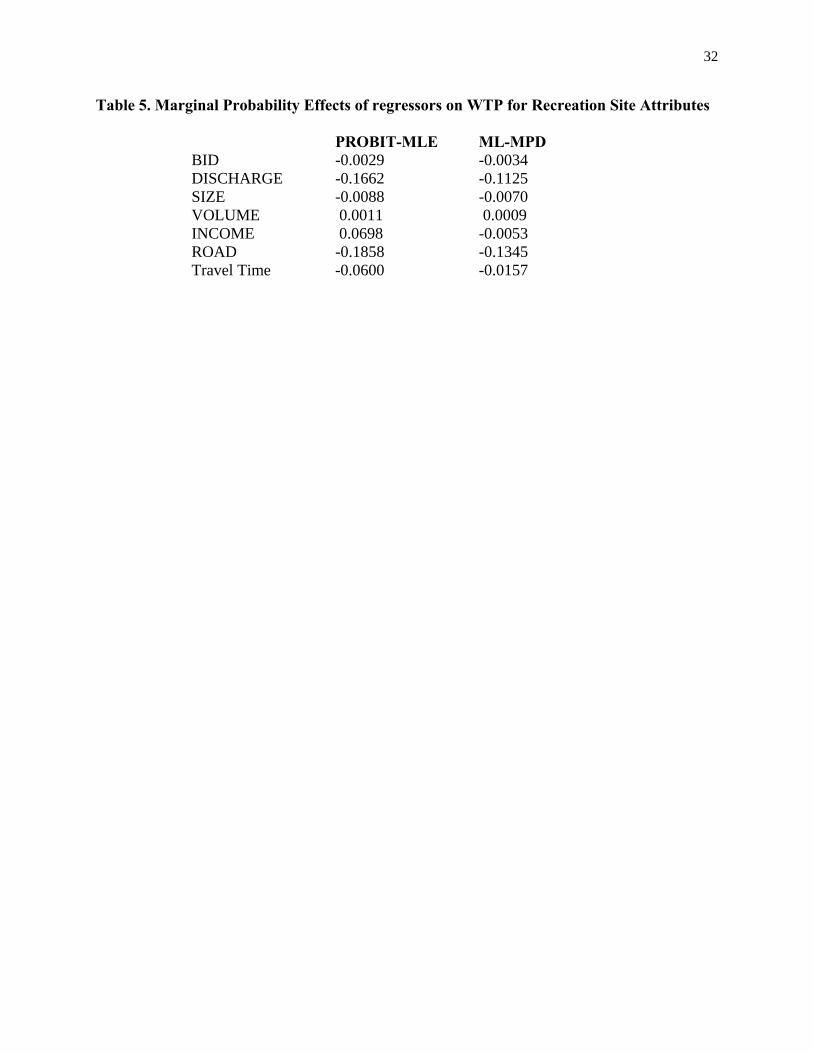
Table 5. Marginal Probability Effects of regressors on WTP for Recreation Site Attributes
PROBIT-MLE ML-MPD BID -0.0029 -0.0034 DISCHARGE -0.1662 -0.1125 SIZE -0.0088 -0.0070 VOLUME 0.0011 0.0009 INCOME 0.0698 -0.0053 ROAD -0.1858 -0.1345 Travel Time -0.0600 -0.0157
33
Figure 1. WTP distribution function and the monotonized empirical survivor function.
0 5 0 1 0 0 1 5 0 2 0 0
0.0
0.2
0.4
0.6
0.8
1.0
b id le ve ls ($ )
W T P D is tr ib utio n F unc tio nM o no to nize d S urvivo r F unc tio n