An Information System for a Bauxite Mine - Informing …proceedings.informingscience.org/InSITE2007/IISITv4p091-104Ever278.pdf · built by “chevron” stacking back and forth, and

An Information System for a Bauxite Mine J. E. Everett

Faculty of Economics and Commerce, University of Western Australia, Crawley, Australia

[email protected]

Abstract Bauxite is mined and transported by conveyor to a processing plant, screened and washed, then placed into blended stockpiles to feed the alumina refinery. While being stacked to the stockpile, the ore is sampled. Completed stockpiles must be acceptably close to target grade (composition), not only in alumina, but also in residual silica, carbon and sodium carbonate.

The mine is an open-cut pit. Each day the choice of ore to mine, from multiple locations in the pit, is based upon estimates of grade. Estimated grade, from exploration drilling of the area before mining, has both systematic and random error.

This paper describes an information system to guide the daily choice of ore to mine. Continually updating the comparison between forecasts and sampled product, the system provides adjusted forecasts. Ore is selected to bring the exponentially smoothed grade to target, in each of the con-trol minerals.

Keywords: MIS, DSS, Mining, Quality Control, Continuous Stockpile Management System, Ex-ponential Smoothing

Introduction Bauxite is the raw material for alumina and aluminium production. In 2004, 56.6 million tonnes of bauxite were mined in Australia, the world’s largest producer. The Australian aluminium in-dustry directly employs over 16,000 people. (Australian Bureau of Statistics, 2006). The International Aluminium Institute, (2000) provides a summary description of the bauxite mining and refining processes.

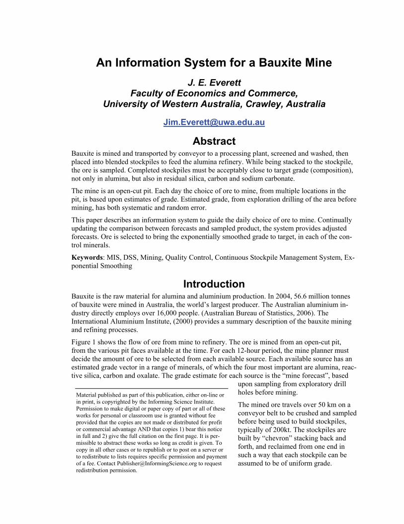
Figure 1 shows the flow of ore from mine to refinery. The ore is mined from an open-cut pit, from the various pit faces available at the time. For each 12-hour period, the mine planner must decide the amount of ore to be selected from each available source. Each available source has an estimated grade vector in a range of minerals, of which the four most important are alumina, reac-tive silica, carbon and oxalate. The grade estimate for each source is the “mine forecast”, based

upon sampling from exploratory drill holes before mining.

The mined ore travels over 50 km on a conveyor belt to be crushed and sampled before being used to build stockpiles, typically of 200kt. The stockpiles are built by “chevron” stacking back and forth, and reclaimed from one end in such a way that each stockpile can be assumed to be of uniform grade.

Material published as part of this publication, either on-line or in print, is copyrighted by the Informing Science Institute. Permission to make digital or paper copy of part or all of these works for personal or classroom use is granted without fee provided that the copies are not made or distributed for profit or commercial advantage AND that copies 1) bear this notice in full and 2) give the full citation on the first page. It is per-missible to abstract these works so long as credit is given. To copy in all other cases or to republish or to post on a server or to redistribute to lists requires specific permission and payment of a fee. Contact [email protected] to request redistribution permission.

Information System for a Bauxite Mine

92

The refinery uses the Bayer process (Habashi, 2005) to convert the bauxite ore to pure alumina. Efficient operation of the refinery depends upon the bauxite feed having consistent grade. It is therefore important that the stockpiles from which the refinery feed is drawn each have grade within a tight range of target, in each of the four minerals.

To achieve the required stockpile grade, the ore selected each day must be chosen appropriately. This is a difficult task, because the ore grade is not known accurately until the ore has been mined, crushed, sampled and assayed. Before mining, the grade of each available source must be forecast from the assays of samples previously taken from quite widely spaced exploration drill holes. An adjusted forecast is calculated, by comparing the recent forecasts with corresponding production sample assays.

Selecting ore to bring each individual stockpile to target requires very tight operational coupling between the mining operation and the building of stockpiles, to ensure that material designed for a particular stockpile goes to that stockpile. The improved system to be described here is opera-tionally decoupled by instead selecting ore each shift so as to bring the exponentially smoothed grade back to target. The Continuous Stockpile Management System (CSMS) being applied was originally developed for iron ore production (Everett, 1996, 2001; Kamperman, Howard & Everett, 2002).

The CSMS achieves operational decoupling but tight information coupling between mining and stockpile building.

In selecting ore to be mined, it is chosen to have adjusted forecast grade such that the exponen-tially smoothed continuous stockpile is as close as possible to target grade. As the ore is mined, the smoothed stockpile grade is updated to incorporate the adjusted forecast grade of the newly mined ore. When that ore is sampled and assayed, the exponentially smoothed continuous stock-pile grade is revised accordingly.

The continuous stockpile grade, and the forecast adjustments are both calculated using exponen-tial smoothing, a widely used forecasting technique (Hanke & Reitsch, 1998). However, the two applications of exponential smoothing differ from each other, and from the usual published appli-cations, as will be described below.

The Continuous Stockpile Discussion with the operating staff confirmed that previous practice had been to attempt to build each individual stockpile to target grade. This led to cyclic behaviour, with weak attention being paid to grade at the start of a stockpile, and strong attention near its completion. Since the build-ing of stockpiles was remote from the mining operation, this required an unachievable tight operational coupling between mining and stockpiling.

Figure 1: The flow of ore from mine to refinery

Conveyor

Stockpiles

RefinerySampling

FeedAvailable Sources

Mine

Everett

93

The next step was to consider a moving average over the stockpile size. For example, since stockpiles are built to 200kt, then the goal is to keep the grade of the most recent 200kt close to target.

Let Pn be the production grade for shift n. Sn is the stockpile grade at shift n, calculated as the moving average over the past k+1 shifts, up to and including shift N. W[n] is the kilotonne pro-duction in shift n. Pn and Sn are vectors, because we are concerned with the grade of the four minerals {bauxite, reactive silica, carbon and oxalate}.

Sn = N-k∑NPn/ N-k∑NW[n], where N-k∑NW[n] = 200 for a 200kt stockpile. (1)

However, a moving average has undesirable informational qualities. Information is treated as equally important until it is suddenly given no further weight. This means that a sudden anomaly generates an appropriate effect when it enters the moving average, but also generates a spurious equal and opposite effect when it leaves the moving average.

A further improvement is to use an exponentially smoothed average. For this, all past information is included, with exponentially declining influence. Let Pń be the exponentially smoothed mean up to and including shift n, smoothed at the exponential rate α1 per kilotonne.

Pń = αnPn + (1-αn)Pń-1 = αnPn + (1-αn)(αn-1Pn-1 +(1-αn-1)(αn-2Pn-2 + …. (2)

In textbook applications of exponential smoothing (e.g. Hanke & Reitsch, 1998) the time (or weight) intervals are generally all the same, so all αn values are identical (and expressed as a). But in the situation being considered here, the tonnage W[n] being mined will vary between shifts, so αn must be adjusted accordingly. It can be shown that the appropriate αn is given by:

αn = 1 – (1- α1)W[n] (3)

For a moving average across a stockpile size of Q kilotonnes, the average “age” of the ore is Q/2 kilotonnes. For an exponentially smoothed stockpile, the average “age” of the ore is 1/a1 kiloton-nes. So to emulate a stockpile size of T kilotonnes we should use a smoothing constant a1 per kilotonne, where:

α1 = 2/Q (4)

Thus, for a CSMS to be equivalent to a stockpile size of 200 kilotonne, α1 should be 0.01 per kilotonne.

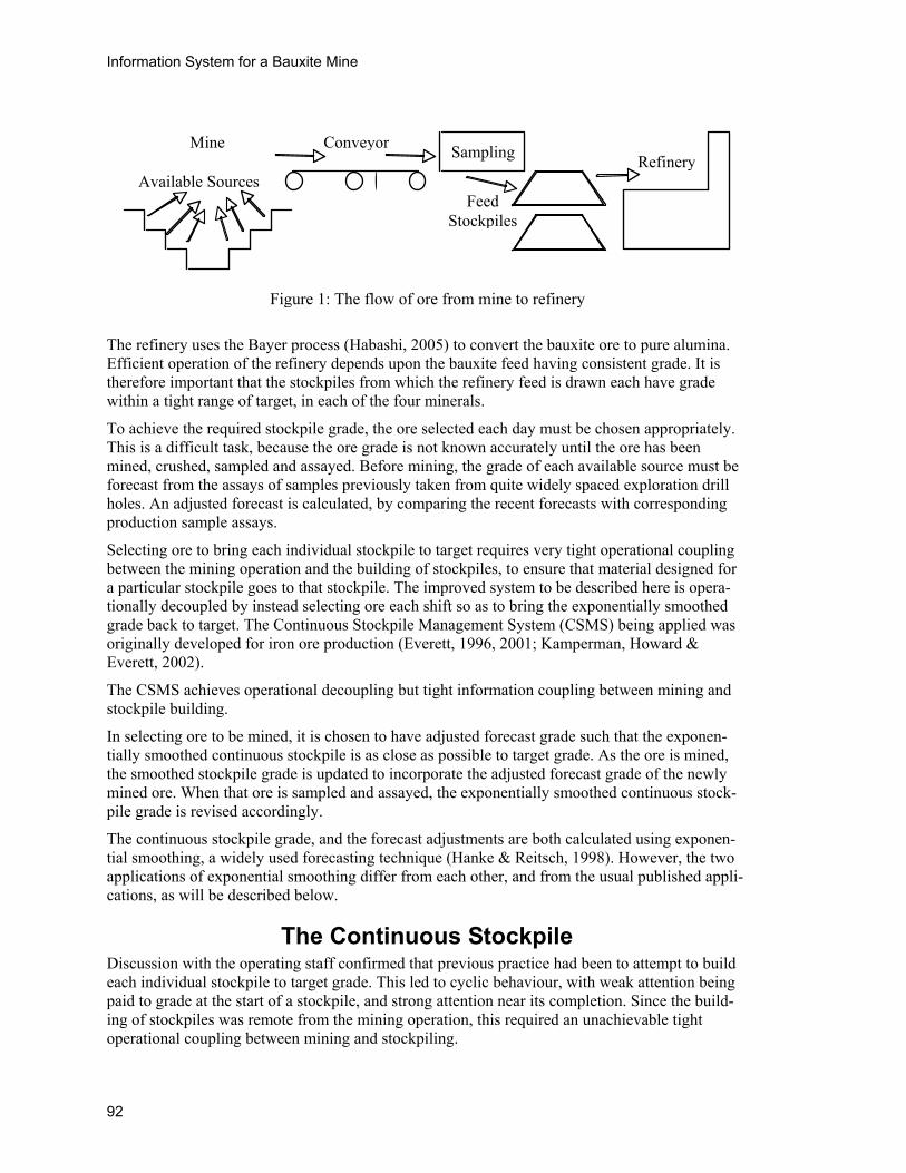
Figure 2 compares moving average and exponential smoothing in the “time” (or tonnage) domain. The effective coefficient applied to a kilotonne of ore is graphed against the tonnage of elapsed ore. The moving average coefficient per kilotonne stays constant until it discontinuously col-lapses to zero, but the exponential smoothing coefficient declines exponentially without discontinuity.

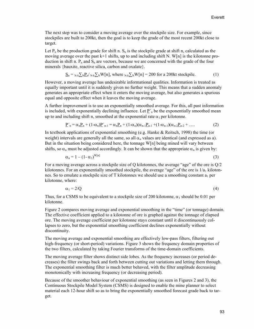
The moving average and exponential smoothing are effectively low-pass filters, filtering out high-frequency (or short-period) variations. Figure 3 shows the frequency domain properties of the two filters, calculated by taking Fourier transforms of the time-domain coefficients.

The moving average filter shows distinct side lobes. As the frequency increases (or period de-creases) the filter swings back and forth between cutting out variations and letting them through. The exponential smoothing filter is much better behaved, with the filter amplitude decreasing monotonically with increasing frequency (or decreasing period).

Because of the smoother behaviour of exponential smoothing (as seen in Figures 2 and 3), the Continuous Stockpile Model System (CSMS) is designed to enable the mine planner to select material each 12-hour shift so as to bring the exponentially smoothed forecast grade back to tar-get.


94

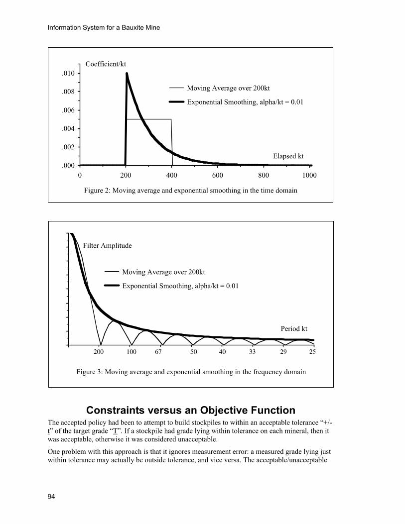
Constraints versus an Objective Function The accepted policy had been to attempt to build stockpiles to within an acceptable tolerance “+/-t” of the target grade “T”. If a stockpile had grade lying within tolerance on each mineral, then it was acceptable, otherwise it was considered unacceptable.

One problem with this approach is that it ignores measurement error: a measured grade lying just within tolerance may actually be outside tolerance, and vice versa. The acceptable/unacceptable

Figure 2: Moving average and exponential smoothing in the time domain

.000

.002

.004

.006

.008

.010

0 200 400 600 800 1000

Moving Average over 200kt

Exponential Smoothing, alpha/kt = 0.01

Coefficient/kt

Elapsed kt

Figure 3: Moving average and exponential smoothing in the frequency domain

Moving Average over 200kt

Exponential Smoothing, alpha/kt = 0.01

Filter Amplitude

Period kt

200 100 67 50 40 33 29 25

Everett

95

discontinuity also makes for a jerky control system, and does not allow for trade-off between the four important mineral components.

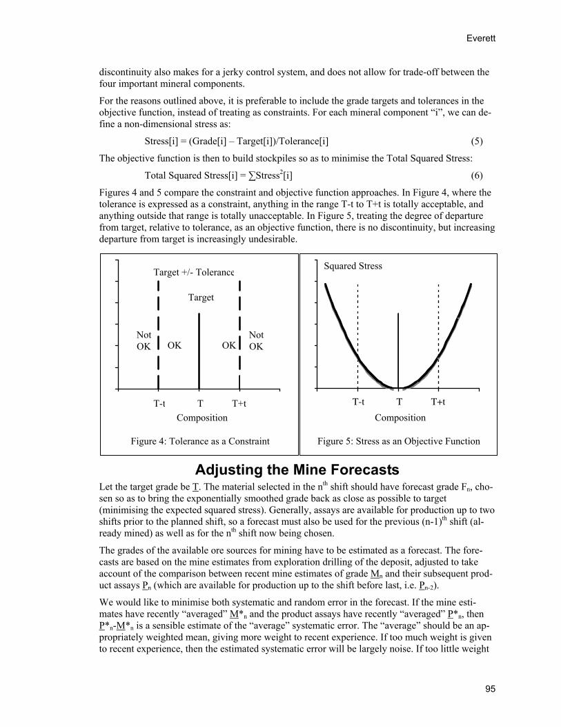
For the reasons outlined above, it is preferable to include the grade targets and tolerances in the objective function, instead of treating as constraints. For each mineral component “i”, we can de-fine a non-dimensional stress as:

Stress[i] = (Grade[i] – Target[i])/Tolerance[i] (5)

The objective function is then to build stockpiles so as to minimise the Total Squared Stress:

Total Squared Stress[i] = ∑Stress2[i] (6)

Figures 4 and 5 compare the constraint and objective function approaches. In Figure 4, where the tolerance is expressed as a constraint, anything in the range T-t to T+t is totally acceptable, and anything outside that range is totally unacceptable. In Figure 5, treating the degree of departure from target, relative to tolerance, as an objective function, there is no discontinuity, but increasing departure from target is increasingly undesirable.

Adjusting the Mine Forecasts Let the target grade be T. The material selected in the nth shift should have forecast grade Fn, cho-sen so as to bring the exponentially smoothed grade back as close as possible to target (minimising the expected squared stress). Generally, assays are available for production up to two shifts prior to the planned shift, so a forecast must also be used for the previous (n-1)th shift (al-ready mined) as well as for the nth shift now being chosen.

The grades of the available ore sources for mining have to be estimated as a forecast. The fore-casts are based on the mine estimates from exploration drilling of the deposit, adjusted to take account of the comparison between recent mine estimates of grade Mn and their subsequent prod-uct assays Pn (which are available for production up to the shift before last, i.e. Pn-2).

We would like to minimise both systematic and random error in the forecast. If the mine esti-mates have recently “averaged” M*n and the product assays have recently “averaged” P*n, then P*n-M*n is a sensible estimate of the “average” systematic error. The “average” should be an ap-propriately weighted mean, giving more weight to recent experience. If too much weight is given to recent experience, then the estimated systematic error will be largely noise. If too little weight

Figure 4: Tolerance as a Constraint

T

OK

T+tT-t

NotOK OK

NotOK

Target

Target +/- Tolerance

Composition

Figure 5: Stress as an Objective Function

T T+tT-t

Composition

Squared Stress


96

is given to recent experience, then the estimated systematic error will be too slow in responding to real changes. Exponential smoothing provides an appropriate method for constructing a weighted history of the systematic error. There is no reason why the appropriate smoothing con-stant (which we shall call β1/kt) should be the same as that for emulating stockpiles (α1/kt). Consequently, we shall use the notation P*n to denote exponential smoothing by β1/kt, whereas Pń denoted exponential smoothing by α1/kt.

For shift n, we are considering selecting ore with mine estimate composition Mn. Product assays are available up to shift n-2. Correcting for systematic error, the adjusted forecast An would be estimated as:

An = Mn + P*n-2 – M*n-2 = P*n-2 + (Mn – M*n-2) (7)

Equation (7) allows for systematic error, but not for random error. If Mn is above average, then Pn is likely to be above average, but by less than is Mn. If Mn is below average, the Pn is likely to be below average, but by less than is Mn. This is a classic regression situation, and equation (7) can be modified to:

An = P*n-2 + r(Mn – M*n-2), where 0 < r < 1 (8)

Equation (8) requires two parameters, the regression coefficient “r”, and the smoothing constant b1/kt. The values of the two parameters are chosen so as to maximise the reduction in error vari-ance:

Error Variance Reduction = 1 – E[(An–Pn)2]/ E[(Mn–Pn)2] (9)

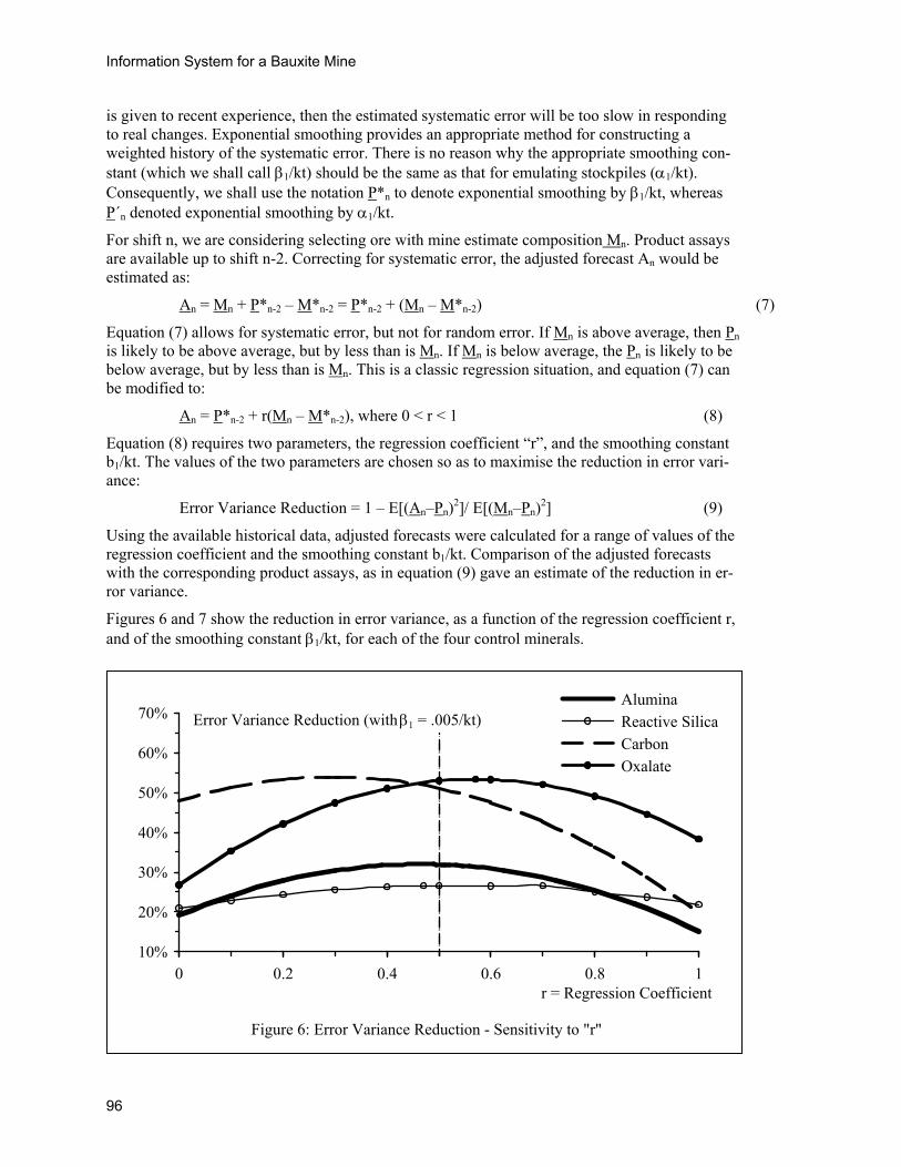
Using the available historical data, adjusted forecasts were calculated for a range of values of the regression coefficient and the smoothing constant b1/kt. Comparison of the adjusted forecasts with the corresponding product assays, as in equation (9) gave an estimate of the reduction in er-ror variance.

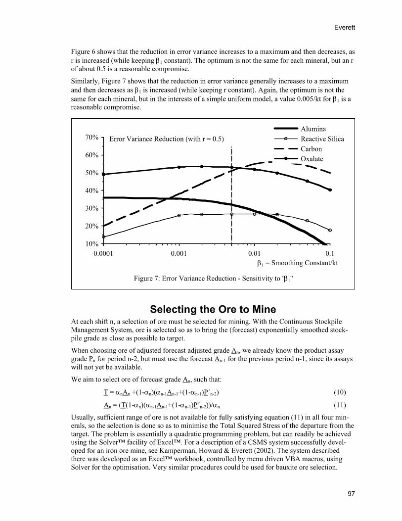
Figures 6 and 7 show the reduction in error variance, as a function of the regression coefficient r, and of the smoothing constant β1/kt, for each of the four control minerals.

Figure 6: Error Variance Reduction - Sensitivity to "r"

10%

20%

30%

40%

50%

60%

70%

0 0.2 0.4 0.6 0.8 1

Alumina Reactive Silica Carbon Oxalate

r = Regression Coefficient

Error Variance Reduction (with β1 = .005/kt)

Everett

97

Figure 6 shows that the reduction in error variance increases to a maximum and then decreases, as r is increased (while keeping β1 constant). The optimum is not the same for each mineral, but an r of about 0.5 is a reasonable compromise.

Similarly, Figure 7 shows that the reduction in error variance generally increases to a maximum and then decreases as β1 is increased (while keeping r constant). Again, the optimum is not the same for each mineral, but in the interests of a simple uniform model, a value 0.005/kt for β1 is a reasonable compromise.

Selecting the Ore to Mine At each shift n, a selection of ore must be selected for mining. With the Continuous Stockpile Management System, ore is selected so as to bring the (forecast) exponentially smoothed stock-pile grade as close as possible to target.

When choosing ore of adjusted forecast adjusted grade An, we already know the product assay grade Pn for period n-2, but must use the forecast An-1 for the previous period n-1, since its assays will not yet be available.

We aim to select ore of forecast grade An, such that:

T = αnAn +(1-αn)(αn-1An-1+(1-αn-1)Pń-2) (10)

An = (T(1-αn)(αn-1An-1+(1-αn-1)Pń-2))/αn (11)

Usually, sufficient range of ore is not available for fully satisfying equation (11) in all four min-erals, so the selection is done so as to minimise the Total Squared Stress of the departure from the target. The problem is essentially a quadratic programming problem, but can readily be achieved using the Solver™ facility of Excel™. For a description of a CSMS system successfully devel-oped for an iron ore mine, see Kamperman, Howard & Everett (2002). The system described there was developed as an Excel™ workbook, controlled by menu driven VBA macros, using Solver for the optimisation. Very similar procedures could be used for bauxite ore selection.

Figure 7: Error Variance Reduction - Sensitivity to "β1"

10%

20%

30%

40%

50%

60%

70%

0.0001 0.001 0.01 0.1

Alumina Reactive Silica Carbon Oxalate

β1 = Smoothing Constant/kt

Error Variance Reduction (with r = 0.5)


98

Simulated Results Data from fifteen months mining operation were analysed. The tonnage mined, mine estimate grades (from exploration drilling) and the final product grades were available for each 12-hour shift. Using the method described above, the adjusted forecasts for each 12-hour production were calculated.

Simulating Actual Production The actual production experience for building 200kt stockpiles was simulated by taking the mov-ing average of the production grade across 200kt of mined ore. This was done by taking a moving average across eleven 12-hour shifts.

Production in each 12-hour shift averaged 18.21kt. So the moving average across eleven 12-hour shifts corresponded to 200.3kt, with a standard deviation of 23.4kt.

Selection of Ore with a CSMS Using Mine Forecasts For the CSMS simulations, it is assumed that ore is selected for each 12-hour shift so as to bring the forecast smoothed composition back to target, as in equations (10) and (11).

Using the original mine forecasts (based upon exploration drilling), the simulation selected ore for each shift to bring the exponentially smoothed grade back to target. This forecast would of course turn out to have an error: the product assay grade was assumed to differ from the mine estimate by the same amount as the actual product grade for that shift differed from the actual mine estimate.

Again, 200kt stockpiles were simulated, by taking the moving average of the simulated product grade, over eleven 12-hour shifts.

Selection of Ore with a CSMS Using Adjusted Forecasts For this CSMS simulation, adjusted forecasts were used to select the ore to be mined each shift. The forecast adjustment was as shown in equation (8), using r = 0.5 and β1 = 0.005/kt.

The forecast error was assumed to be the same as the difference between the product grade and the adjusted forecast grade for the same actual shift.

Again, 200kt stockpiles were simulated, by taking the moving average of the simulated product grade, over eleven 12-hour shifts.

The results of the three sets of simulations are graphed below, for alumina, residual silica, carbon and oxalate.

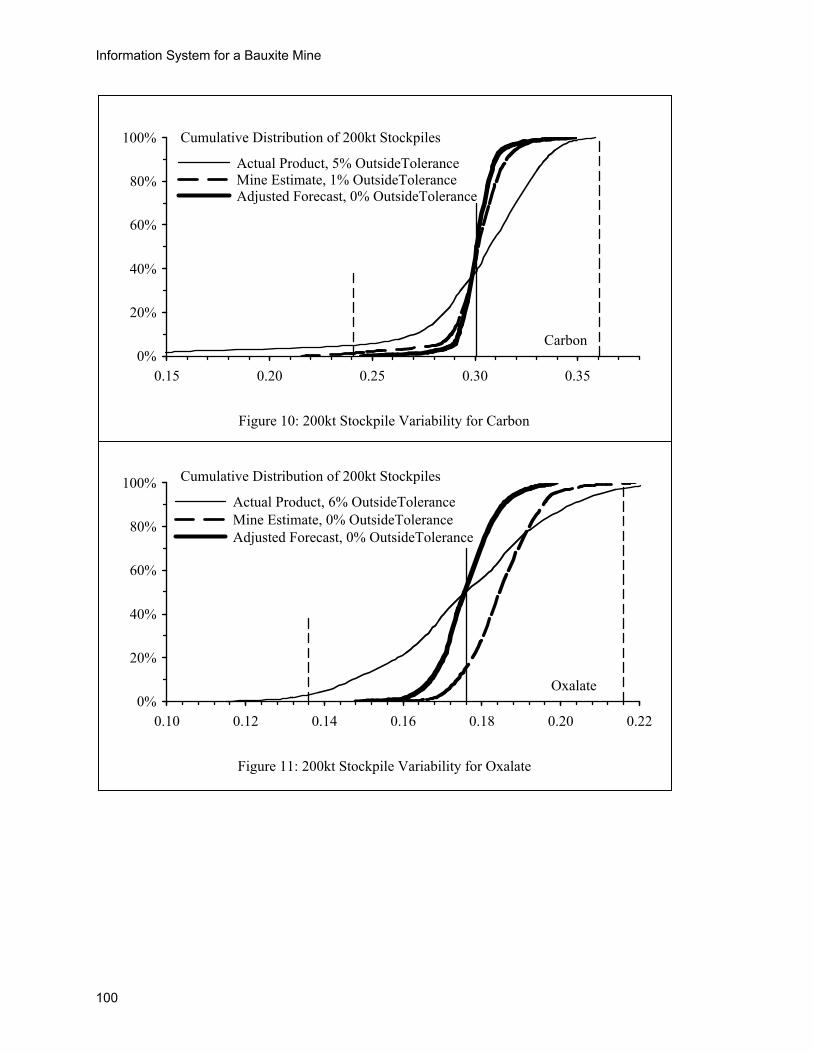
Comparing the Three Simulations Figures 8 to 11 show comparisons of the three simulations for each of the four minerals of inter-est.

In Figure 8, the thin line shows the cumulative distribution of the alumina grade of actual stock-piles, built under the previous grade control procedures. About 18% of the completed stockpiles were below the tolerance, and a similar proportion above the tolerance limit, giving a total of 31% of completed stockpiles outside the tolerance range in alumina. If the Continuous Stockpile Man-agement System (CSMS) had been adopted, using the mine estimates to select ore for mining, so as to restore the continuous stockpile grade to target, then only 24% of stockpiles would have been outside tolerance in the alumina grade, as shown by the thick broken line. If the CSMS had

Everett

99

been used, with adjusted forecasts to guide ore selection, then the proportion of completed stock-piles outside tolerance would have been further reduced to only 10%.

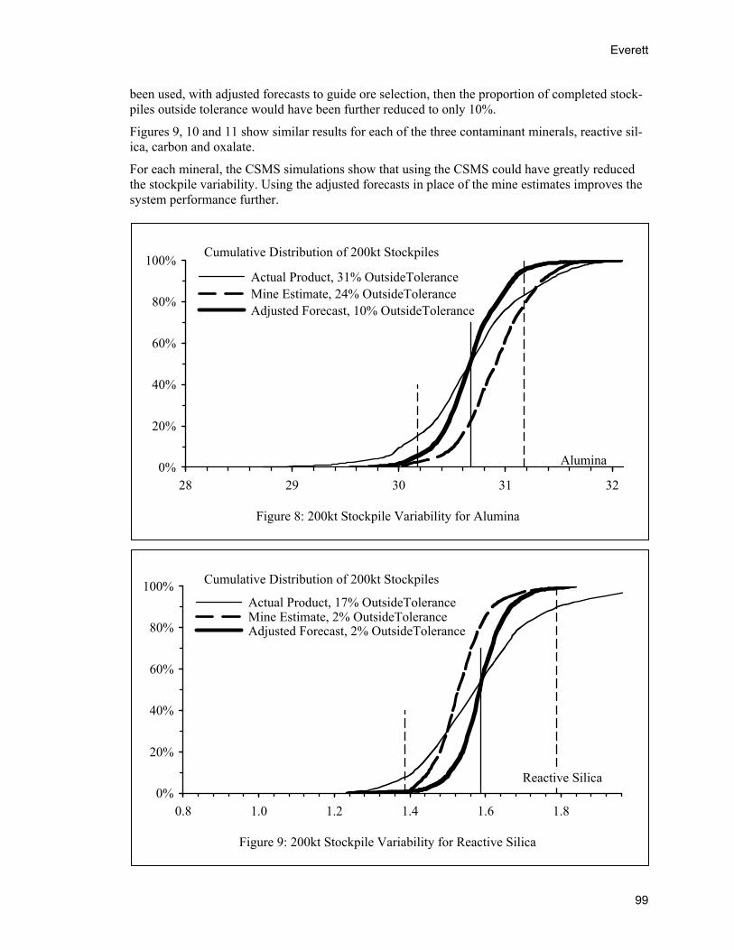
Figures 9, 10 and 11 show similar results for each of the three contaminant minerals, reactive sil-ica, carbon and oxalate.

For each mineral, the CSMS simulations show that using the CSMS could have greatly reduced the stockpile variability. Using the adjusted forecasts in place of the mine estimates improves the system performance further.

Figure 9: 200kt Stockpile Variability for Reactive Silica

0%

20%

40%

60%

80%

100%

0.8 1.0 1.2 1.4 1.6 1.8

Actual Product, 17% OutsideTolerance Mine Estimate, 2% OutsideTolerance Adjusted Forecast, 2% OutsideTolerance

Cumulative Distribution of 200kt Stockpiles

Reactive Silica

Figure 8: 200kt Stockpile Variability for Alumina

0%

20%

40%

60%

80%

100%

28 29 30 31 32



Alumina


100

Figure 10: 200kt Stockpile Variability for Carbon

0%

20%

40%

60%

80%

100%

0.15 0.20 0.25 0.30 0.35



Carbon

Figure 11: 200kt Stockpile Variability for Oxalate

0%

20%

40%

60%

80%

100%

0.10 0.12 0.14 0.16 0.18 0.20 0.22



Oxalate

Everett

101

Effect of Stockpile Size Increasing the stockpile size will decrease the stockpile grade variability. If the ore grade had no serial correlation, then the decrease in stockpile variability would be proportional to the square root of the stockpile size, so quadrupling stockpile size would halve the stockpile grade standard deviation. However, ore grades have a positive serial correlation (high grades tend to be followed by high grades in the short term, and vice versa) so the decrease with stockpile size is actually slower.

Larger stockpile sizes were simulated, by taking moving averages over more than eleven shifts. Each shift averages 18.21 kt, so a stockpile size of 255 kt can be simulated by taking moving av-erages across fourteen shifts, a stockpile size of 310 kt by moving averages across 17 shifts, and so on.

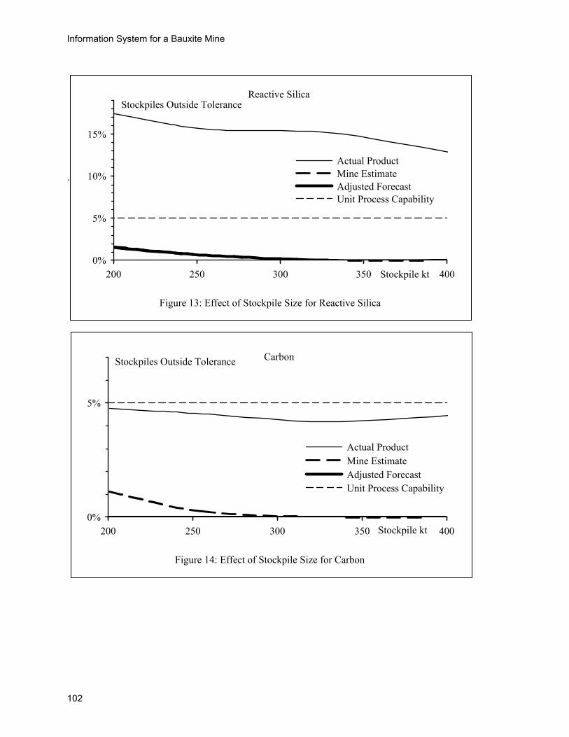
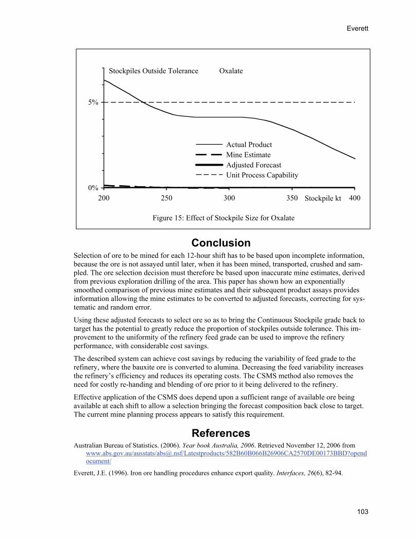
Figures 12 to 15 plot the proportion of stockpiles against stockpile size. For the purposes of this paper, “Process capability” is defined as the tolerance range divided by the 95% confidence limit. With unit process capability, 5% of stockpiles lie outside tolerance, a reasonable operational goal.

In the Figures 12 to 15, simulations for the actual product are shown as thin solid lines. Simula-tions of the CSMS, with ore selection guided by mine estimates and by adjusted forecasts are shown by broken and by solid thick lines respectively.

Figures 12 and 13 show that increasing the stockpile size would not achieve unit process capabil-ity for alumina or for reactive silica, using the actual product generated by the previous ore selection procedure. For a CSMS with ore selected using adjusted forecasts, unit process capabil-ity for alumina could be achieved with a stockpile size of 250kt. For the three contaminating minerals, (reactive silica, carbon and oxalate, shown in Figures 13, 14 and 15 respectively) the CSMS would yield better than unit process capability even for the current 200kt stockpile size.

Figure 12: Effect of Stockpile Size for Alumina

0%

5%

10%

15%

20%

25%

30%

200 250 300 350 400

Actual Product Mine Estimate Adjusted Forecast Unit Process Capability

Stockpile kt

Stockpiles Outside Tolerance Alumina


102

.

Figure 13: Effect of Stockpile Size for Reactive Silica

0%

5%

10%

15%

200 250 300 350 400


Stockpile kt

Stockpiles Outside ToleranceReactive Silica

Figure 14: Effect of Stockpile Size for Carbon

0%

5%

200 250 300 350 400


Stockpile kt

Stockpiles Outside Tolerance Carbon

Everett

103

Conclusion Selection of ore to be mined for each 12-hour shift has to be based upon incomplete information, because the ore is not assayed until later, when it has been mined, transported, crushed and sam-pled. The ore selection decision must therefore be based upon inaccurate mine estimates, derived from previous exploration drilling of the area. This paper has shown how an exponentially smoothed comparison of previous mine estimates and their subsequent product assays provides information allowing the mine estimates to be converted to adjusted forecasts, correcting for sys-tematic and random error.

Using these adjusted forecasts to select ore so as to bring the Continuous Stockpile grade back to target has the potential to greatly reduce the proportion of stockpiles outside tolerance. This im-provement to the uniformity of the refinery feed grade can be used to improve the refinery performance, with considerable cost savings.

The described system can achieve cost savings by reducing the variability of feed grade to the refinery, where the bauxite ore is converted to alumina. Decreasing the feed variability increases the refinery’s efficiency and reduces its operating costs. The CSMS method also removes the need for costly re-handing and blending of ore prior to it being delivered to the refinery.

Effective application of the CSMS does depend upon a sufficient range of available ore being available at each shift to allow a selection bringing the forecast composition back close to target. The current mine planning process appears to satisfy this requirement.

References Australian Bureau of Statistics. (2006). Year book Australia, 2006. Retrieved November 12, 2006 from

www.abs.gov.au/ausstats/[email protected]/Latestproducts/582B60B066B26906CA2570DE00173BBD?opendocument/

Everett, J.E. (1996). Iron ore handling procedures enhance export quality. Interfaces, 26(6), 82-94.

Figure 15: Effect of Stockpile Size for Oxalate

0%

5%

200 250 300 350 400


Stockpile kt

Stockpiles Outside Tolerance Oxalate


104

Everett, J.E. (2001). Iron ore production scheduling to improve product quality. European Journal of Op-erational Research, 129, 355-361.

Habashi, F. (2005). A short history of hydrometallurgy. Hydrometallurgy, 79, 15-22.

Hanke, J.E. & Reitsch, A.G. (1998). Business forecasting (6th ed.). Englewood Cliffs: Prentice-Hall.

International Aluminium Institute. (2000). World-Aluminium.Org. Retrieved November 12, 2006 from www.world-aluminium.org/production/mining/index.html

Kamperman, M., Howard, T. & Everett, J.E. (2002). Controlling product quality at high production rates. In R. Holmes (Ed.), Proceedings of the Iron Ore 2002 Conference, Perth, Western Australia, 9-11 September 2002. Carlton, Victoria: Australasian Inst. of Mining and Metallurgy. ISBN 1 875776 94 X, 255-260.

Biography Jim Everett began as a research geophysicist at Cambridge and the Australian National University. His family always said “what are you going to do when you grow up”, so he joined industry, as a petroleum exploration geophysicist. With a computer background, he was put onto project evaluations. Losing arguments with accountants, he did a couple of Economics and Commerce degrees at the University of Western Australia (and found that the accountants were usually right). The university was then starting its MBA course and wanted people with industry experience to teach on it. With a young family, fieldwork was no longer so attractive, so Jim jumped at the chance of returning to academia. Thirty years on, he has now retired as Emeritus Professor of

Information Management, and divides his time between research and consulting to Western Aus-tralia’s booming mining industry.

Documents

An Information System for a Bauxite Mine - Informing …proceedings.informingscience.org/InSITE2007/IISITv4p091-104Ever278.pdf · built by “chevron” stacking back and forth, and