Embed Size (px)
Citation preview

Chalmers University of Technology
University of Gothenburg
Department of Computer Science and Engineering
Göteborg, Sweden, June 2010
An Improved Static-Priority Scheduling Algorithm
for Multi-Processor Real-Time Systems
Master of Science Thesis in Secure and Dependable Computer System
CHAO XU
YING DING

The Authors grant to Chalmers University of Technology and University of Gothenburg
the non-exclusive right to publish the Work electronically and in a non-commercial
purpose make it accessible on the Internet.
The Authors warrant that they are the authors to the Work, and warrants that the Work
does not contain text, pictures or other material that violates copyright law.
The Authors shall, when transferring the rights of the Work to a third party (for example a
publisher or a company), acknowledge the third party about this agreement. If the Authors
have signed a copyright agreement with a third party regarding the Work, the Authors
warrant hereby that they have obtained any necessary permission from this third party to
let Chalmers University of Technology and University of Gothenburg store the Work
electronically and make it accessible on the Internet.
An Improved Static-Priority Scheduling Algorithm for Multi-Processor Real-Time
Systems
Chao Xu
Ying Ding
© Chao Xu, June 2010.
© Ying Ding, June 2010.
Examiner: Jan Jonsson
Chalmers University of Technology
University of Gothenburg
Department of Computer Science and Engineering
SE-412 96 Göteborg
Sweden
Telephone + 46 (0)31-772 1000
Cover: The picture is generated by using www.wordle.net
Department of Computer Science and Engineering
Göteborg, Sweden June 2010

An Improved Static-Priority Scheduling Algorithm for
Multi-Processor Real-time Systems
Chao Xu, Ying Ding
Department Computer Science Engineering
Chalmers University of Technology
Abstract
This thesis deals with the problem of designing a new real-time scheduling algorithm
for independent periodic tasks with static priority on multi-processor platforms called
IBSP-TS (Interval Based Semi-Partitioned Task Splitting). The widely implemented
priority policy Rate-Monotonic is applied in the algorithm. IBSP-TS combines
interval-based semi-partition technique and another multi-processor scheduling
algorithm SPA2 to achieve the highest possible worst-case utilization bound to ln2
while meeting the deadlines.
The assignment of IBSP is divided into two parts. In the first part, tasks are
categorized into several interval groups. Each group has its own assignment policy
except for the last interval. In most cases, there are some tasks residual after applying
all the policies. All the residual tasks are handled along with the tasks from last
interval in the second part of the algorithm. The schedulability can be ensured by
feasibility tests.
The simulation experiment shows IBSP-TS has some good properties compared to the
best static-priority multi-processor scheduling algorithm at this moment. It generally
has higher success ratio, less sorted tasks and also less task migrations. In the best
case, it can achieve the break-down utilization point to 76% in simulation.
Additionally, this algorithm can let system designer to choose the number of intervals
in the algorithm. The more intervals, the less number of sorted tasks there are.
Keywords: Real-Time Scheduling, Utilization Bound, Multi-Processor, Static-Priority,
Rate-Monotonic, Periodic, Preemptive, Semi-Partitioned, Task Splitting


Acknowledgement
First of all, we would like to thank our thesis examiner Docent Jan Jonsson. It is
because of his excellent teaching in real-time system and his deep and wide
knowledge in this field which leaded us into the research of this thesis.
Equivalently, we owe our greatest gratitude to Mr. Risat Mahmud Pathan for his
cordial help. Without him, this thesis would not have been possible. He had made
available his support in number of ways, such as his invaluable ideas, his timely
feedback and his guidance. All these not only provide us inspirations, but also give us
confidence in our research.
Additionally, it is a pleasure to thank all the friends around us who had inspired us
and gave us suggestions.
Finally, we would like to show our gratitude to our parents for their encouragement
and understanding.
Chao Xu, Ying Ding


Content
I Introduction ............................................................................................................................... 1
1.1 Contributions ................................................................................................................. 2
1.2 Thesis Outline ............................................................................................................... 2
II Related Background .................................................................................................................. 5
2.1 Real-Time Tasks ............................................................................................................ 5
2.1.1 Task Parameters ................................................................................................ 6
2.1.2 Task Priorities .................................................................................................... 7
2.2 Utilization Bound .......................................................................................................... 7
2.3 Scheduling Feasibility Analysis .................................................................................... 8
2.4 Scheduling Features ...................................................................................................... 9
2.4.1 Preemptive vs. Non-Preemptive ........................................................................ 9
2.4.2 Static vs. Dynamic ............................................................................................ 9
2.4.3 Uniprocessor vs. Multi-Processor ................................................................... 10
2.5 Multi-Processor Scheduling ........................................................................................ 11
2.5.1 Global Scheduling ........................................................................................... 11
2.5.2 Partitioned Scheduling .................................................................................... 12
2.5.3 Semi-Partitioned Scheduling ........................................................................... 13
III Models and Assumptions ................................................................................................ 17
3.1 System Model ............................................................................................................. 17
3.2 Task Model .................................................................................................................. 17
IV IBSP-TS Algorithm ......................................................................................................... 19
4.1 Overview ..................................................................................................................... 19
4.2 Phase One .................................................................................................................... 19
4.2.1 Intervals and Policies ...................................................................................... 19
4.2.2 Non-Parallel Execution ................................................................................... 30
4.3 Phase Two ................................................................................................................... 35
4.3.1 Assignment Procedure .................................................................................... 35
4.3.2 Non-Parallel Execution ................................................................................... 36

Content
4.4 Utilization Bound ........................................................................................................ 37
4.5 Pseudo Code ................................................................................................................ 37
4.6 Assignment Example .................................................................................................. 39
V Evaluation ............................................................................................................................... 43
5.1 Simulation Setup ......................................................................................................... 43
5.2 Simulation Result ........................................................................................................ 45
VI Conclusion ...................................................................................................................... 59
Bibliography ................................................................................................................................... 61
Appendix ......................................................................................................................................... 65

1
I
Introduction
It has already become the truth that people’s life relies more and more on computers.
Computers systems are ubiquitous. It can range from the smallest PDA device to
super-computer. Some of them need high performance; some of them may require
fault tolerance; and some of them have strong timing constraints. For a computer
system with strong timing constraints, it is called real-time systems. The chief design
goal of real-time system is not high throughput, but rather a guarantee of the
consistency concerning the amount of time its applications take. Therefore, the
correctness of a real-time system is not only logical and functional, but also temporal.
In real world, there are always some critical issues that have to be processed within a
fixed amount of time whenever invoked. For example, mechanical systems on
production lines, breaking systems in vehicles, flying systems in aircrafts and space
shuttles, E-commerce systems in stock exchanges and consoles in nuclear power
plants, all these need real-time system to ensure the temporal correctness.
All the real-time system can be categorized into two groups, hard real-time systems
and soft real-time systems. In hard real-time systems, the consequences of not
fulfilling a time constraint may be catastrophic, such as medical systems. Hence,
predictability is paramount among all concerns. On the other hand, for soft real-time
systems, single failures of not fulfilling a time constraint is acceptable, examples of
soft real-time systems are multimedia systems and communication systems.
Moore’s Law mentioned that the number of transistors per area unit on a integrate
circuit doubles approximately every two years. It is certain that, with faster processors,
system designers can use the increased capacity to deliver better services.
Nevertheless, a fast computer is not enough to ensure real-time properties. Therefore,
utilizing the resource as much as possible and ensuring real-time processing lead to a
research of real-time scheduling. For the time being, real-time scheduling for

2 Introduction
uniprocessor is quite mature. Meanwhile, the development for multi-core processor is
impressive these years. In 2009, even a processor with 100-core was released [1].
However, those well-developed scheduling algorithms for uniprocessor perform
poorly in multi-processor systems in the term of worst-case utilization bound. It is
proved that only 50% can be achieved [2]. Therefore, developing new algorithms for
multi-processor received considerable attention these years.
Recently, there is a static-priority scheduling algorithm for multi-processor systems –
IBPS [3] has been proposed. Tasks with the range (0, 1] are categorized into seven
intervals to achieve a worst-case utilization bound as 55.2%.Later, another scheduling
algorithm for multi-processor systems called the SPA2 [4], has theoretically proved
that the worst-case utilization bound for static-priority multi-processor scheduling can
achieve to ln2, which is the highest possible value. However, the SPA2 algorithm has
to sort all the tasks in a task set which is not applicable for online scheduling.
Additionally, SPA2 suffers from the number of subtasks from an individual task,
which can bring considerable context switch in a system.
In this paper, a new static-priority scheduling algorithm for multi-processor systems
scheduling called IBSP-TS is proposed, which is an interval based semi-partitioned
scheduling algorithm. It tries to assign as many tasks as possible to a single processor.
However, if a task cannot be fully assigned to a single processor, it will be split into
one or more subtasks. IBSP-TS combinations the ideas from IBPS algorithm and
SPA2 algorithm to reach the same worst-case schedulable utilization bound as ln2.
Meanwhile, it reduces the number of preemptions and migrations for practical use and
holds a higher schedulable rate than SPA2.
1.1 Contributions
The main contributions of this thesis are as follows:
1. IBSP-TS achieve the highest possible worst-case utilization bound of a
static-priority multi-processor scheduling to ln2.
2. Online scheduling is possible with IBSP-TS
3. There are less overhead for IBSP compared to SPA2 algorithm.
4. For mixed tasks and heavy utilization tasks, IBSP-TS has better schedulability
than SPA2.
5. It is possible for the system designer to choose the number of intervals in
IBSP-TS. The more intervals, the less sorted tasks are.
1.2 Thesis Outline
The rest of this thesis is organized as follows:
Introduction 3
Chapter II describes the related background of real-time scheduling.
Chapter III presents the necessary assumption and models of tasks and the system
be used in new algorithm IBSP-TS.
The design details of IBSP-TS algorithm are shown in Chapter IV.
In Chapter V, the performance of IBSP-TS is estimated by comparing with
another algorithm SPA2.
Finally, Chapter VI concludes this thesis with a discussion on the applicability
and extendibility of IBSP-TS algorithm.

4 Introduction

5
II
Related Background
In this section, the related background of real-time scheduling is presented, such as
what are real-time tasks, including its parameters and priorities; how is utilization
bound defined; what is scheduling feasibility test; what is the difference between
different scheduling schemes; and various multi-processor scheduling algorithms.
2.1 Real-Time Tasks
A task is unit of work such as a program or code-block that when executed provides
some service of an application. It can be either dependent or independent. For a
dependent task, its execution may require an exclusive access to a shared resource
(e.g., a file, a data structure in shared memory or an external device other than
processor time) or it has some precedence constraints. If a resource is shared among
multiple tasks, then some tasks may be blocked from being executed until the shared
resource is free. Similarly, if tasks have precedence constraints, then one task may
need to wait until another task finishes its execution. A region of code with such a
requirement is called a critical section. Tasks are said to be independent when they
have no critical sections. In this thesis, each task is assumed to be independent in the
sense that it does not interact in any manner (accessing shared data, exchanging
messages, etc.) with other tasks. The only resource the tasks share is the processor
platform.
A real-time task is a task running in real-time system. In general, a real-time task may
require a specific amount of particular resource during a specific period of time. A
real-time task system can be classified in as periodic task, aperiodic tasks or sporadic
tasks.
A periodic task is a task that arrives with a continuous and deterministic pattern of

6 Related Background
time interval. That is, it continuously requests resources at time values. In addition to
this requirement, a real-time periodic task must complete processing by a specified
deadline relative to the time that it acquires the processor.
An aperiodic task is a stream of jobs arriving irregularly. There may either be no
bound or only a statistical bound on the arrival period. It requests a resource during
non-deterministic request periods. Each task job is also associated with a specified
deadline, which represents the time necessary for it to complete its execution.
A sporadic task is an aperiodic task with a hard deadline and a minimum inter-arrival
time.
In this thesis, it is assumed that only periodic tasks are considered.
2.1.1 Task Parameters
A task set is a set of n independent periodic tasks denoted as .
An independent periodic task can be fully characterized by the following
parameters.
Period ( ): Each task in periodic task system has an inter-arrival time of
occurrence, called the period of the task. In each period, a job of the task, which
is the recurrent copy of the task, is released.
Offset ( ): A task is ready to execute at the beginning of each period, called the
released time, of the task. The first job of a task may arrive at any time-instant; an
offset defines the release time of the first job. If the relative deadline of each task
in a task set is less than or equal to its period, then the task set is called a
constrained deadline periodic task system. If the relative deadline of each task in
a constrained deadline task set is exactly equal to its period, then the task set is
called an implicit deadline periodic task system. If a periodic task system is
neither constrained nor implicit, then it is called an arbitrary deadline periodic
task system. In this thesis, scheduling of implicit deadline periodic task system is
considered.
Deadline ( ): Each job of a task has a relative deadline that that defines the time
window in which the job has to be executed since its release time. The relative
deadlines of all the jobs of a particular periodic task are same. The absolute
deadline of a job is the time instant equal to released time plus the relative
deadline.
WCET (worst-case execution time) ( ): Each periodic task has a WCET that is
the maximum execution time that each job of the task requires.

Related Background 7
Utilization ( ): The utilization of a task is actually the utilization of processor for
a task, which is the ratio of the execution time of a task to its period.
2.1.2 Task Priorities
In a periodic task system, all that are released but have not complete their individual
execution by the time t are called active tasks. When two or more active tasks
compete for a same processor, some rules must be applied to for the scheduling
dispatcher to allocate the use of the processor. It assigns priorities to all tasks that are
eligible for execution and then selects the highest priority one on a processor. The
priority of a task can be static or dynamic.
For static-priority scheduling, priorities never change once they are assigned. Hence,
each job of a task inherits its initial priority. Static-priority scheduling dispatchers are
inherently memoryless in that the prioritization of tasks is independent of previous
scheduling decisions. Rate-monotonic (RM) scheduling [5] is an example of such a
policy for periodic and sporadic tasks. Under the RM prioritization, tasks with shorter
periods are given higher priority.
Under dynamic-priority discipline, the priority order of an active task may be changed
during its execution. For different jobs of a task may have different priorities relative
to other tasks in the system. Earliest-deadline-first (EDF) scheduling [5] is a
dynamic-priority policy often considered for scheduling periodic and sporadic tasks.
It gives jobs with earlier absolute deadlines with higher priority.
When a task is released at time t, its execution may be delayed due to other higher
priority tasks running in the system. In RM scheduling, a task with smaller period has
higher priority. In case, two tasks have exactly the same period, they have equal
priority, which means the scheduling dispatcher can randomly pick either of them.
In this thesis, the RM scheduling priority is adopted.
2.2 Utilization Bound
A processor is said to be fully utilized when an increase in the computation time of
any of the tasks in a task set will make the task set unschedulable. The least upper
bound of the total utilization is the minimum of all total utilizations over all sets of
tasks that fully utilize the processor. This least upper bound of a scheduling algorithm
is called the worst-case utilization bound (minimum achievable utilization bound) or
simply utilization bound of the scheduling algorithm. A scheduling algorithm can
feasibly schedule any set of tasks on a processor if the total utilization of the tasks is
less than or equal to the utilization bound of the scheduling algorithm. For example, in
uniprocessor scheduling, the utilization bound of RM is 69% and the utilization bound

8 Related Background
of EDF is 100% [5].
2.3 Scheduling Feasibility Analysis
To predict the temporal behavior and to determine whether the timing constraints of
an application tasks will be met during runtime, feasibility analysis of scheduling
algorithm is conducted. A schedule is said to be feasible if it fulfills all application
constraints for a given set of tasks. A set of tasks is said to be schedulable if there
exists at least one scheduling algorithm that can generate a feasible schedule. A
scheduling algorithm is said to be optimal with respect to schedulability if it can
always find a feasible schedule whenever any other scheduling algorithm can do so.
Feasibility analysis of a hard real-time system refers to the process of determining
offline whether the specified system will meet all deadlines at runtime. A feasibility
test is introduced by doing feasibility analysis. It uses one or several conditions to
determine whether a task set is feasible for a given scheduling algorithm. The
feasibility test can be necessary and sufficient or only sufficient.
For a sufficient feasibility test, a task set pass the test shows that it is definitely
schedulable. However, if a task set does not pass the sufficient feasibility test, it may
still be schedulable. While, for a necessary and sufficient feasibility test, if and only if
a task set pass test, its tasks can meet their individual deadlines.
Processor utilization analysis is one of the techniques to perform the feasibility test. It
uses the sum of utilizations of all the tasks belong to the set, that is . While, in
multi-processor system, system utilization is often used which represent the utilization
of a task set on m processors.
In 1973, Liu and Layland derived a sufficient feasibility test for RM scheduling and
an exact test for EDF scheduling on uniprocessor.
A set of n tasks is schedulable by the RM algorithm if
.
For the EDF algorithm, a set of n periodic tasks is schedulable if and only if
.
In 2001, another test is presented which is called hyperbolic test [6] for
Rate-Monotonic scheduling. It dominates the bound of Liu & Layland for RM, but it

Related Background 9
has the same effect as Liu & Layland Test if there are infinite numbers of tasks on a
processor.
2.4 Scheduling Features
When the number of tasks does not exceed the number of processors, each task can
simply be assigned a dedicated processor. However, usually this is not the case. At
least one processor must be shared among multiple tasks. Therefore, the most
important part of real-time system design is to choose a good scheduling scheme
which can fulfill the application constraints. In the following part, various scheduling
schemes are presented. In this thesis, IBSP-TS are defined as a preemptive static
priority multi-processor scheduling algorithm.
2.4.1 Preemptive vs. Non-Preemptive
A scheduling algorithm is preemptive if the release of a new job of a higher priority
task can preempt the job of a currently running lower priority task. During runtime,
task scheduling is essentially determining the highest priority active tasks and
executing them in the free processor. For example, RM and EDF are examples of
preemptive scheduling algorithm.
On the contrary, in non-preemptive scheme, a currently executing task always
completes its execution before another active task starts execution. Therefore, in
non-preemptive scheduling a higher priority active task may need to wait in the ready
queue until the currently executing task (may be of lower priority) completes its
execution.
A preemptive scheduling algorithm can succeed in meeting deadlines where a
non-preemptive scheduling algorithm fails but a non-preemptive scheduling algorithm
has naturally the advantage of no run-time overhead caused by preemptions. In this
thesis, only preemptive scheduling is considered.
2.4.2 Static vs. Dynamic
The scheduling can be generated offline or online, which represent static (offline)
scheduling and dynamic (online) scheduling separately.
When the complete schedulability analysis of a task system can be done before the

10 Related Background
system is put in mission, the scheduling is considered as static scheduling. Scheduling
dispatcher holds a time table, which contains explicit start and completion times for
each task job that controls the order of execution at run-time. In order to predict
feasibility of a task set, static scheduling analysis requires the availability of all static
task parameters, like periods, execution time, and deadlines.
Dynamic scheduling makes scheduling decisions at each time-instant based upon the
characteristics of the task that have arrived so far. It has no knowledge of tasks that
may arrive in the future. Since a newly arriving task can interfere with the execution
of already existing tasks in the system, an admission controller is needed to determine
whether to accept a new task that arrives online. The feasibility test of a scheduling
algorithm can be used as the basis for designing an admission controller for dynamic
systems. However, evaluating the feasibility test when a new task arrives must not
take too long time. This is because using processing capacity to do the feasibility test
could detrimentally affect the timing constraints of the existing tasks in the system.
2.4.3 Uniprocessor vs. Multi-Processor
Real-time scheduling theorists have extensively studied for hard real-time scheduling
with uniprocessor. Uniprocessor scheduling algorithm executes tasks on a single
processor. The schedulability of a given set of tasks on uniprocessor platform can be
determined by using Liu and Layland Test. It is well known that RM and EDF are
optimal algorithms for uniprocessor scheduling.
At this point, it is worth to mention that the RM algorithm is widely used in industry
because of its simplicity, flexibility and its ease of implementation [7, 8]. It can be
used to satisfy the stringent timing constraints of tasks; while at the same time it can
also support execution of a-periodic tasks and meet the deadlines of the periodic tasks.
RM can be modified easily, for example, to implement priority inheritance protocol
for synchronization purpose [9]. The conclusion of the study in [7] is that “...the
Rate-Monotonic algorithm is a simple algorithm which is not only easy to implement
but also very versatile”.
Multi-core processors are quickly emerging as the dominant technology in the
microprocessor industry. Major chip manufacturers have already adopted multi-core
technologies due to the thermal problems that distress traditional single-core chip
designs in terms of processor performance and power consumption. In 2009, even a
100-core processor had been released [1]. Recently, many steps have been taken
towards obtaining a better understanding of hard real-time scheduling on
multi-processors.
As multi-processor systems have faster computational power and fault-tolerance
feature, use of multi-processor and distributed systems in real-time applications is
becoming popular. As compared to scheduling real-time tasks on a uniprocessor,

Related Background 11
scheduling tasks on multi-processor and distributed systems is a much more
challenging problem.
2.5 Multi-Processor Scheduling
Multi-processor scheduling algorithms are often categorized as global scheduling and
partitioned scheduling. However, it has been proved that neither global nor
partitioned static-priority multi-processor scheduling algorithm can achieve a
utilization bound greater than 50% [2]. Therefore, in order to achieve utilization
bound greater than 50%, another new category called semi-partitioned scheduling
comes out recently, which introduces the technique task splitting into the traditional
partitioned scheduling algorithm. In the following part, each of them is presented.
2.5.1 Global Scheduling
Global scheduling algorithms store tasks which have arrived but execution unfinished
in one queue that is shared by all processors. In other words, the highest priority task
is always selected to be executed whenever the scheduling dispatcher is invoked,
regardless of which processor is being scheduled. At every moment,the m highest
priority tasks among those are selected for execution on the m processors. In addition,
task preemptions and migrations are permitted, that is a task preempted on a particular
processor may resume execution on the same or on a different processor. Due to this,
global scheduling on average utilizes computing resource well.
Proportionate-fair (Pfair) scheduling [10, 11] is a global scheduling approach
proposed as a means for optimally scheduling periodic tasks on multi-processors.
Pfair scheduling uses a quantum-based model. In Pfair scheduling, although a task has
started executing, lower priority tasks receive a guaranteed time quantum per time
unit for execution, all tasks hence make some kind of progress per time unit. It is
known that PF [10], PD [11] and PD2 [12] are optimal Pfair algorithms which can
theoretically achieve 100% schedulable system utilization. The PD2 is known to be
the most efficient in the optimal Pfair algorithms. LLREF algorithm [13] which is
based on a different technique relying on the original notation called T-L Plane (Time
and Local Execution Time Domain Plane), can also achieve 100% schedulable system
utilization.
However, these algorithms will generate a number of task preemptions and migration
overhead and they are very complex to implement. There are some simple global
dynamic priority scheduling algorithms which perform fairly well with a small
number of task preemptions and migration overhead, such as EDF-US[1/2] [14, 15]
scheduling policy. It gives only a few high-utilization tasks top priority; all other tasks
are scheduled according to deadlines. EDZL (Earliest Deadline Zero Laxity) [16] is a
hybrid preemptive dynamic priority scheduling scheme in which tasks with zero
laxity are given highest priority and other tasks are ranked by deadline. Nevertheless,

12 Related Background
their utilization bounds for schedulable systems are down to 50%.
As applies to static priority scheduling, it is known that Rate-Monotonic priority
assignment scheme is not optimal for multi-processor systems, because global RM
can miss deadline even utilization approaches zero [17].
RM-US [m/(3m-2)] [18] algorithm (m is the number of processors) can guarantee
schedulability as long as the multiprocessor utilization is below 33%. Later, an
improved version RM-US [0.37482] [19] guarantees schedulability for all systems up
to 37.482% for the system utilization. These two algorithms categorize a task as
heavy or light. A task is said to be heavy if the utilization exceeds a certain threshold
number and a task is said to be light otherwise. Heavy tasks are assigned with higher
priority and the light tasks are assigned with lower priority. The relative priority order
among light tasks is given by RM.
Nowadays, the best known utilization bound of global static-priority scheduling is
38%, which is reached by SM-US [2/(3+√5)] (Slack Monotonic) [20]. It uses similar
priority scheduling scheme which categorizes tasks as heavy and light and assigns the
highest priority to heavy tasks. The relative priority order of light tasks is given by
SM, which means task is assigned higher priority than task if
.
Later, another global scheduling algorithm WM (Weight-Monotonic) [21] was
proposed and has been proved that the worst-case utilization bound is 50% [18].
However, the WM algorithm generates a large number of task preemptions due to the
characteristic of Pfair scheduling.
2.5.2 Partitioned Scheduling
The alternative to global scheduling is partitioned scheduling. It partition a task set
into groups beforehand. Each processor holds a separate ready queue such that each
task group which is assigned to a specific processor. In other words, during the run
time, tasks may not migrate from one processor to another. Thus, multi-processor
scheduling is equivalent to multiple uniprocessor systems.
The predominant approach of scheduling multi-processor hard real-time systems is
usually for partitioned scheduling, since it has the virtue of applying efficient
uniprocessor techniques on each processor. As no task migrations occur in partitioned
scheduling, it is superior to global in practice. Additionally, the schedulability of
partitioned scheduling can be verified by using well-understood uniprocessor analysis
techniques.
The most well known static priority scheduling algorithm is RM-FF [22], which use
First-fit bin-packing algorithm. For First-fit, it means that tasks are assigned into in
increasing index order visited processors. It has been proved by Oh & Baker that the

Related Background 13
utilization guarantee bound in RMFF for a system with m processors using the is
between and [23]. The lower bound shows
that the worst-case utilization bound is 41%. Another algorithm, RM-FFDU (First-Fit
Decreasing Utilization) [24], which conducts the FF heuristic after sorting the tasks in
decreasing utilization order; it usually performs better than RM-FF algorithm.
Thereafter, another static priority scheduling algorithm called R-BOUND-MP-NFR
(multi-processor next-fit-ring) [2] is presented with the best result of partitioned
static-priority scheduling reaching 50%. It introduces the NFR heuristic into the
R-BOUND-MP algorithm. Here, R-BOUND-MP is a previously known
multi-processor scheduling algorithm which combines R-BOUND [25] with First-fit
bin-packing algorithm and exploits R-BOUND.
Additionally, there are some simple dynamic-priority scheduling algorithms, such as
EDF-FF (Earliest Deadline First-Fit) [26] and EDF-BF (Earliest Deadline Best-Fit)
[26]. For best-fit, it means a task is assigned to a processor which verify the
schedulability test after assignment and which maximizes the remaining processor
capacity. The system utilization bounds of these algorithms are also 50%, but these
partitioned scheduling algorithms can reduce more preemptions and task migration
overhead than global scheduling algorithms.
2.5.3 Semi-Partitioned Scheduling
It has been proved that neither global nor partitioned static-priority multi-processor
scheduling algorithm can achieve a utilization bound greater than 50% [2]. Therefore,
nowadays a lot of work has been done on semi-partitioned scheduling in order to
achieve utilization bound higher than 50%. Semi-partitioned scheduling algorithms
introduce techniques such as task splitting into the traditional partitioned scheduling
algorithm. When the spare capacity of the individual processor is not enough to fully
accept the execution of a task, it split the task into two or more pieces. Each piece is
called a subtask and to a dedicated processor. In other words, this task execution is
allowed to migrate to different processors. Meanwhile, most tasks are statically
assigned to one fixed processor as in traditional partitioned scheduling. Here, the most
important condition is that no subtasks split from one task run in parallel. In such a
way that a task never returns to the same processor within the same period once it is
migrated from one processor to another processor.
RMDP (Rate-Monotonic Deferrable Portion) [27] is a static priority scheduling
algorithm based on the semi-portioned scheduling technique and reaches to the
worst-case utilization bound as 50%. In RMDP, tasks are sorted in increasing period
order and assigned to processors sequentially. If a task t makes the total utilization of
a processor P exceed its utilization bound, the task is split into two parts. The first part
is assigned to that processor P, and the second part is assigned to the next chosen
processor.

14 Related Background
DM-PM (Deadline Monotonic-Priority Migration), [28] an algorithm based on the
concept of semi-partitioned scheduling also achieves utilization bound higher than
50%. In DM-PM algorithm, each task is assigned to a particular processor by using
some kinds of bin-packing heuristics, upon which the schedulable condition for DM is
satisfied. If there are no such processors, DM-PM shares the task with more than one
processor. By doing this, an unfeasible task with classical partitioned approaches can
be scheduled.
a task is qualified to migrate only if it cannot be assigned to any individual processors.
Another static-priority scheduling algorithm – IBPS (Interval Based Partitioned
Scheduling) [3] has been proposed with system utilization bound 55.2%. In IBPS,
tasks are grouped into seven utilization intervals and then the tasks from these groups
are assigned to processors using different policies. As IBPS has only two subtasks, the
total number of migrations caused by split tasks is lower than of any other
task-splitting algorithm.
In a later work, a partitioned scheduling algorithm – PDMS-HPTS (Partitioned
Deadline Monotonic Scheduling - Highest Priority Task Splitting) [29] with task
splitting technique used on the highest priority task can lead to a utilization bound of
60%. A specific instance of this class, where tasks are allocated in the decreasing
order of sizes using PDMS-HPTS-DS [29] can achieves system utilization bound of
65% theoretically. The utilization bound of 69.3% is achieved when the utilization of
each individual task is restrictively less than 41.4%. Additionally, it has shown that
the utilization bound of PDMS-HPTS-DS in simulation can reach to 88% in practice
In term of worst-case utilization bound, the best algorithm for multi-processor with
static priority so far is SPA2 (Semi-Partitioned Algorithm 2), which has theoretically
shows the utilization bound of 69.3% in worst case [4]. In SPA2, tasks are categorized
into heavy tasks and light tasks. For heavy tasks, there is a pre-assigning mechanism.
For light tasks, the algorithm assigns tasks in decreasing period order, and always
selects the processor with the least workload assigned so far among all processors, to
assign the next task.
Task splitting technology can also be applied to dynamic-priority scheduling, for
example, the well known EKG (EDF with task splitting and K processors in a Group.)
[12] and Ehd2-SIP (EDF with Highest priority Deferrable portion-2 task-Sequential
assignment in Increasing Period) [30] which improves schedulability with a few
preemptions.
EKG assigns each task to a particular processor like conventional partitioned
scheduling algorithms. However, it can split a task into parts if necessary. It assigns
the first part to the current processor on which the assignment is going and the second
part to the next picked processor. The two parts of a split task are scheduled

Related Background 15
exclusively. The least upper bound of the schedulable system utilization for EKG
depends on the value of a parameter k which should be selected in the range of
where M is the number of processors in a system. A large k results in a
higher bound but more preemptions. The bound becomes 66% in the case of k=2 and
100% in the case of k=M. Namely EKG is an optimal algorithm in the case of k=M,
although there are more preemptions[30].
The Ehd2-SIP algorithm takes a similar approach to EKG in such a way that each task
is classified into a fixed task or a migratable task, and the approach is more simplified
for practical use. While EKG utilizes the full capacity of every processor on which a
migratable task is executed, Ehd2-SIP does not fully utilize the processor to reduce
the computation complexity. Thus, the scheduling of migratable tasks is more
straightforward than EKG. Although it can often successfully schedule a task set with
system utilization much higher than 50%, the utilization bound is 50%. From the
viewpoint of balance between schedulability and complexity, Ehd2-SIP and EKG with
small parameter k are attractive.
Another presented algorithm EDDP [31] integrates the notions of Ehd2-SIP and EKG.
In EDDP, the deadline of a split task is changed to a smaller deadline called “virtual
deadline”. EDDP succeeds the design simplicity of Ehd2-SIP for practical use; and at
the same time, it partially imitates the approach of EKG but with an improved system
utilization bound. The advantage of EDDP is that the implementation cost is not far
beyond the traditional partitioned scheduling algorithms, while the worst-case system
utilization bound is no less than 65%.
Moreover, an algorithm called EDHS (Earliest Deadline Highest priority Split) [32]
based on EDF also uses the task splitting techniques. The only difference between
EDHS and those previous splitting techniques is that the tasks are never split as long
as they can be partitioned. It has been proved that EDHS algorithm improves
schedulable multi-processor utilization by 10 to 30% over the traditional partitioning
approach.
In this thesis, the presented algorithm IBSP-TS combines the idea of IBPS [3] and
SPA2 [4]. It has the highest possible worst-case utilization bound as ln2 and
dominates all other static-priority multi-processor scheduling algorithms except for
the SPA algorithm which also achieved to ln2. Nevertheless, IBSP-TS has some other
advantages over SPA2, such as less task migrations, less number of sorted tasks.

16 Related Background
Figure 1: Design space of multi-processor real-time scheduling
Figure 1 shows all the multi-processor real-time scheduling algorithms in existing
literature. As it shows that multiprocessor real-time scheduling can be categorized into
global scheduling, partitioned scheduling and semi-partitioned scheduling. Each of
these categories can be divided into static priority scheduling algorithm and dynamic
priority scheduling algorithm. In global scheduling sub-group, there is a special
family called Pfair scheduling algorithm. The last layer of this figure shows that the
highest utilization bound of that category.

17
III
Models & Assumptions
In this section, the definition of the system and tasks used by IBSP-TS algorithm is
presented. All the assumptions and configuration in the system are critical for
designing a real-time scheduling algorithm. In this thesis, the scheduling problem is
referring to the assignment of n independent, periodically arrived real-time tasks on m
identical processors in Rate-Monotonic priory.
3.1 System Model
The system used in this thesis is a memory shared multi-processor system composed
of m processors, P1, P2, ... , Pm. Each processor within the multi-processor system is
identical. All code and data of tasks are shared among all processors. The overhead of
inter-processor is negligible, which means there is no task migration cost for the
schedulability test. Whereas, the number of context switches is counted as a metric of
algorithm performance.
3.2 Task Model
The system has a task set of n periodic tasks denoted as . All
these tasks are independent and preemptive. Moreover, there is no synchronization
among tasks. No jobs of a task or subtasks can be executed on two or more processors
simultaneously, and a processor cannot execute two or more tasks simultaneously.
Jobs of the same task must be executed sequentially which means that every job of
is not allowed to run before the preceding job of completes.

18 Models & Assumptions
Each task from this task set is characterized by a pair of parameters .
represents the period of the task and is the WCET . For periodic tasks, its
relative deadlines are equals to its period. Every time a task arrives, a job of the
task is created to denote the k-th copy of the task. A task is released and ready for
execution at every time . The task utilization , is the ration of its execution time to
its period,
.
Furthermore, a task can be split into two or more subtasks ,
,…, which
means a task execution can be migrated to more than one processors. The sum of the
execution time of all those subtasks split from one task is exactly equals to the ’s
execution time, that is
. The period of a subtask inherits from its
original task. Thus, the utilization of a subtask becomes
The total utilization of a task set (system utilization) which is defined as the sum of
utilizations of all the tasks belong to the set (in a system), that is . All these
parameters of a task are not allowed to modify except for subtasks, which split the
execution time to several parts.

19
IV
IBSP-TS Algorithm
In this section, assignment approach and task splitting in IBSP-TS algorithm are
presented in detail. Moreover, non-parallel execution of subtasks is shown step by
step with mathematic proof. Additionally, pseudo-code and a task assignment example
are listed in order to give a more clear understanding of the algorithm.
4.1 Overview
The task assignment is divided into two phases so as to reach the best possible
worst-case utilization bound as ln2. Task utilization set (0, 1] is divided into i disjoint
subsets called utilization intervals . Tasks from each interval are
assigned to some processors using a particular policy for . By doing this, not only
the utilization bound can be achieved to ln2 in each processor, but also the number of
tasks left unassigned after applying these policies can be reduced. Any task
unassigned in and tasks from the last interval are assigned to processors in
by using SPA2 [4]. The more intervals, the less left unassigned tasks left for sorting
which is good for online scheduling. Therefore, it is a trade-off between the number
of intervals and the number of sorting tasks.
In this thesis, 27 disjoint utilization intervals . The unassigned task in intervals
and tasks from the last interval are assigned by using SPA2.
4.2 Phase One
4.2.1 Intervals and Policies
Lemma 1: In Phase One, each processor has the worst-case utilization strictly

20 IBSP-TS Algorithm
greater than ln2 and all the tasks on the processor can meet their deadlines.
Proof: The utilization range (0, 1] is divided into twenty-seven disjoint utilization
intervals , which is described in the following Table 1. Each interval defined by
( ], which means when a task belongs to this interval, its utilization is less or
equal to and strictly greater than
Table 1: 27 disjoint utilization intervals -
Furthermore, twenty-seven different policies applied in intervals . The upper
bound of an interval equals to the lower bound of latest previous interval. According
to Hyperbolic Test for RM scheduling , if

IBSP-TS Algorithm 21
all n tasks on a processor can meet their deadlines. The details of policies are defined
are as follow.
1. All tasks with utilization greater than ln2 are assigned to one processor exclusively.
Thus, . Therefore, each task is assigned to one
dedicated processor and no more tasks left from this interval.
2. Exactly five tasks
are assigned to four processors. Among
these five tasks, the highest priority one is selected and split it into four subtasks.
Each task set {
} is assigned to one processor.
All the tasks assigned by this policy meet their deadlines according to Hyperbolic
Bound Test:
All the processors used in this policy maintain utilization bound greater than ln2:
Thus, there may be 0 4 tasks left in this interval after Phase One.
3. Exactly three tasks
are assigned to two processors.
Among these three tasks, the highest priority one is selected and split it into two
subtasks. Each task set {
} is assigned to one processor.
All the tasks assigned by this policy meet their deadlines according to Hyperbolic
Bound Test:
All the processors used in this policy maintain utilization bound greater than ln2:
Thus, there may be 0 2 tasks left in this interval after Phase One.
4. Exactly five tasks
are assigned to three processors. Two
tasks out of these five which has higher priority are split into two subtasks, one is
and the other is
. Task sets {
}, {
} and {
} are
assigned to a single processor separately.
All the tasks assigned by this policy meet their deadlines according to Hyperbolic
Bound Test:

22 IBSP-TS Algorithm
Since, it has a set
in a processor. Thus, another test is needed to ensure
the schedulability.
All the processors used in this policy maintain utilization bound greater than ln2:
Thus, there may be 0 4 tasks left in this interval after Phase One.
5. Exactly seven tasks
are assigned to four processors.
Three tasks out of these seven which has higher priority are split into two subtasks,
one is
and the other is
. Task sets {
}, {
}, {
} and
{
} are assigned to a single processor separately.
All the tasks assigned by this policy meet their deadlines according to Hyperbolic
Bound Test:
Since
, it has a set
in a processor. Thus, another test is needed.
All the processors used in this policy maintain utilization bound greater than ln2:
Thus, there may be 0 6 tasks left in this interval after Phase One.
6. Exactly two tasks
are assigned to one processor.
All the tasks assigned by this policy meet their deadlines according to Hyperbolic
Bound Test:
All the processors used in this policy maintain utilization bound greater than ln2:

IBSP-TS Algorithm 23
Thus, there may be 0 1 tasks left in this interval after Phase One.
7. Exactly nine tasks
are assigned to four processors.
Among these nine tasks, the highest priority one is selected and split it into four
subtasks. Each task set {
} is assigned to one processor.
All the tasks assigned by this policy meet their deadlines according to Hyperbolic
Bound Test:
All the processors used in this policy maintain utilization bound greater than ln2:
Thus, there may be 0~8 tasks left in this interval after Phase One.
8. Exactly five tasks
are assigned to two processors.
Among these five tasks, the highest priority one is selected and split it into two
subtasks. Each task set {
} is assigned to one processor.
All the tasks assigned by this policy meet their deadlines according to Hyperbolic
Bound Test:
All the processors used in this policy maintain utilization bound greater than ln2:
Thus, there may be 0 4 tasks left in this interval after Phase One.
9. Exactly eleven tasks
are assigned to four processors.
Three tasks out of these eleven which has higher priority are split into two
subtasks, one is
and the other is
. Task sets {
}, {
},
{
} and {
} are assigned to a single processor
separately.
All the tasks assigned by this policy meet their deadlines according to Hyperbolic
Bound Test:
Since
, it has a set
in a processor. Thus, another test is needed.

24 IBSP-TS Algorithm
All the processors used in this policy maintain utilization bound greater than ln2:
Thus, there may be 0 10 tasks left in this interval after Phase One.
10. Exactly three tasks
are assigned to one processor.
All the tasks assigned by this policy meet their deadlines according to Hyperbolic
Bound Test:
All the processors used in this policy maintain utilization bound greater than ln2:
Thus, there may be 0 2 tasks left in this interval after Phase One.
11. Exactly thirteen tasks
are assigned to four processors.
Among these thirteen tasks, the highest priority one is selected and split it into
four subtasks. Each task set {
} is assigned to one processor.
All the tasks assigned by this policy meet their deadlines according to Hyperbolic
Bound Test:
All the processors used in this policy maintain utilization bound greater than ln2:
Thus, there may be 0 12 tasks left in this interval after Phase One.
12. Exactly seven tasks
are assigned to two processors.
Among these seven tasks, the highest priority one is selected and split it into two
subtasks. Each task set {
} is assigned to one processor.
All the tasks assigned by this policy meet their deadlines according to Hyperbolic
Bound Test:
All the processors used in this policy maintain utilization bound greater than ln2:

IBSP-TS Algorithm 25
Thus, there may be 0 6 tasks left in this interval after Phase One.
13. Exactly eleven tasks
are assigned to three processors.
Two tasks out of these five which has higher priority are split into two subtasks,
one is
and the other is
. Task sets {
}, {
} and
{
} are assigned to a single processor separately.
All the tasks assigned by this policy meet their deadlines according to Hyperbolic
Bound Test:
Since
, it has a set
in a processor. Thus, another test is needed.
All the processors used in this policy maintain utilization bound greater than ln2:
Thus, there may be 0 10 tasks left in this interval after Phase One.
14. Exactly four tasks
are assigned to one processor.
All the tasks assigned by this policy meet their deadlines according to Hyperbolic
Bound Test:
All the processors used in this policy maintain utilization bound greater than ln2:
Thus, there may be 0 tasks left in this interval after Phase One.
15. Exactly seventeen tasks
are assigned to four
processors. Among these seventeen tasks, the highest priority one is selected and
split it into four subtasks. Each task set {
} is assigned to one
processor.
All the tasks assigned by this policy meet their deadlines according to Hyperbolic
Bound Test:

26 IBSP-TS Algorithm
All the processors used in this policy maintain utilization bound greater than ln2:
Thus, there may be 0 16 tasks left in this interval after Phase One.
16. Exactly nine tasks
are assigned to two processors.
Among these nine tasks, the highest priority one is selected and split it into two
subtasks. Each task set {
} is assigned to one processor.
All the tasks assigned by this policy meet their deadlines according to Hyperbolic
Bound Test:
All the processors used in this policy maintain utilization bound greater than ln2:
Thus, there may be 0 8 tasks left in this interval after Phase One.
17. Exactly fourteen tasks
are assigned to three processors.
Two tasks out of these fourteen which has higher priority are split into two
subtasks, one is
and the other is
. Task sets {
},
{
} and {
} are assigned to a single
processor separately.
All the tasks assigned by this policy meet their deadlines according to Hyperbolic
Bound Test:
Since
, it has a set
in a processor. Thus, another test is needed.
All the processors used in this policy maintain utilization bound greater than ln2:
Thus, there may be 0 13 tasks left in this interval after Phase One.

IBSP-TS Algorithm 27
18. Exactly five tasks
are assigned to one processor.
All the tasks assigned by this policy meet their deadlines according to Hyperbolic
Bound Test:
All the processors used in this policy maintain utilization bound greater than ln2:
Thus, there may be 0 4 tasks left in this interval after Phase One.
19. Exactly twenty one tasks
are assigned to four
processors. Among these twenty one tasks, the highest priority one is selected and
split it into four subtasks. Each task set {
} is assigned to one
processor.
All the tasks assigned by this policy meet their deadlines according to Hyperbolic
Bound Test:
All the processors used in this policy maintain utilization bound greater than ln2:
Thus, there may be 0 20 tasks left in this interval after Phase One.
20. Exactly eleven tasks
are assigned to two processors.
Among these eleven tasks, the highest priority one is selected and split it into two
subtasks. Each task set {
} is assigned to one processor.
All the tasks assigned by this policy meet their deadlines according to Hyperbolic
Bound Test:
All the processors used in this policy maintain utilization bound greater than ln2:
Thus, there may be 0 10 tasks left in this interval after Phase One.
21. Exactly seventeen tasks
are assigned to three
processors. Two tasks out of these five which has higher priority are split into two

28 IBSP-TS Algorithm
subtasks, one is
and the other is
. Task sets {
},
{
} and {
} are assigned to a
single processor.
All the tasks assigned by this policy meet their deadlines according to Hyperbolic
Bound Test:
Since
, it has a set
in a processor. Thus, another test is needed.
All the processors used in this policy maintain utilization bound greater than ln2:
Thus, there may be 0 16 tasks left in this interval after Phase One.
22. Exactly six tasks
are assigned to one processor.
All the tasks assigned by this policy meet their deadlines according to Hyperbolic
Bound Test:
All the processors used in this policy maintain utilization bound greater than ln2:
Thus, there may be 0 5 tasks left in this interval after Phase One.
23. Exactly twenty five tasks
are assigned to four
processors. Among these twenty five tasks, the highest priority one is selected and
split it into four subtasks. Each task set {
} is assigned to
one processor.
All the tasks assigned by this policy meet their deadlines according to Hyperbolic
Bound Test:
All the processors used in this policy maintain utilization bound greater than ln2:

IBSP-TS Algorithm 29
Thus, there may be 0 24 tasks left in this interval after Phase One.
24. Exactly thirteen tasks
are assigned to two processors.
Among these eleven tasks, the highest priority one is selected and split it into two
subtasks. Each task set {
} is assigned to one processor.
All the tasks assigned by this policy meet their deadlines according to Hyperbolic
Bound Test:
All the processors used in this policy maintain utilization bound greater than ln2:
Thus, there may be 0 12 tasks left in this interval after Phase One.
25. Exactly twenty tasks
are assigned to three processors.
Two tasks out of these five which has higher priority are split into two subtasks,
one is
and the other is
. Task sets {
},
{
} and {
} are assigned
to a single processor.
All the tasks assigned by this policy meet their deadlines according to Hyperbolic
Bound Test:
Since
, it has a set
in a processor. Thus, another test is needed.
All the processors used in this policy maintain utilization bound greater than ln2:
Thus, there may be 0 19 tasks left in this interval after Phase One.
26. Exactly seven tasks
are assigned to one processor.
All the tasks assigned by this policy meet their deadlines according to Hyperbolic
Bound Test:
All the processors used in this policy maintain utilization bound greater than ln2:
30 IBSP-TS Algorithm
Thus, there may be 0 6 tasks left in this interval after Phase One.
27. The left interval which is
. Assign tasks which have utilization less
than
along with all the unassigned tasks left which are called residual tasks
after Phase One in Phase Two by using SPA2.
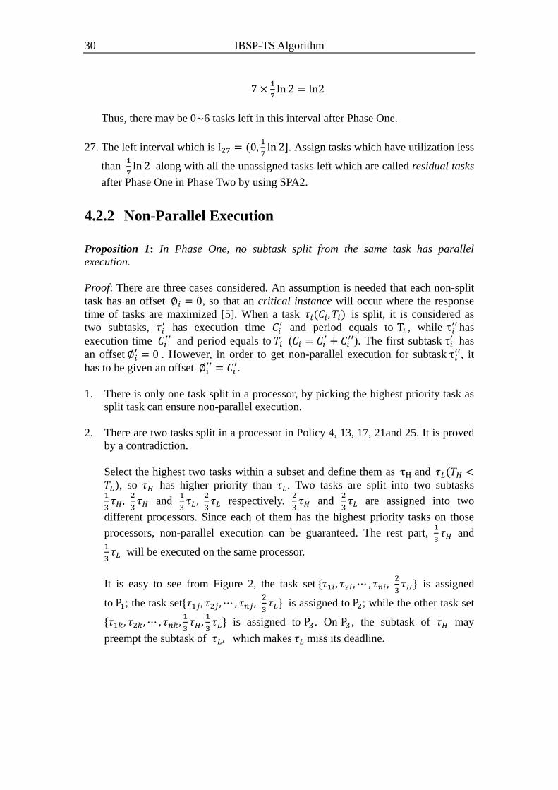
4.2.2 Non-Parallel Execution
Proposition 1: In Phase One, no subtask split from the same task has parallel
execution.
Proof: There are three cases considered. An assumption is needed that each non-split
task has an offset , so that an critical instance will occur where the response
time of tasks are maximized [5]. When a task is split, it is considered as
two subtasks, has execution time
and period equals to , while has
execution time and period equals to (
). The first subtask
has
an offset . However, in order to get non-parallel execution for subtask
, it
has to be given an offset
.
1. There is only one task split in a processor, by picking the highest priority task as
split task can ensure non-parallel execution.
2. There are two tasks split in a processor in Policy 4, 13, 17, 21and 25. It is proved
by a contradiction.
Select the highest two tasks within a subset and define them as and , so has higher priority than . Two tasks are split into two subtasks
and
respectively.
and
are assigned into two
different processors. Since each of them has the highest priority tasks on those
processors, non-parallel execution can be guaranteed. The rest part,
and
will be executed on the same processor.
It is easy to see from Figure 2, the task set
is assigned
to ; the task set
is assigned to ; while the other task set
is assigned to . On , the subtask of may
preempt the subtask of which makes miss its deadline.

IBSP-TS Algorithm 31
Figure 2: Example of scheduling two
and
on one processor
Assume that the subtask of misses its deadline, the execution time of these
two split tasks is respectively represented as and . The response time of
goes as follows
Intervals Conditions Testing Procedure
A contradiction is derived, so
will meet its deadline.

32 IBSP-TS Algorithm
A contradiction is derived, so
will meet its deadline.
A contradiction is derived, so
will meet its deadline.
A contradiction is derived, so
will meet its deadline.
A contradiction is derived, so
will meet its deadline.
Table 2: Non-parallel execution proof for two split tasks
Table 2 shows the contradictions in each different interval. It is clear that
3. There are three tasks split in a processor in Policy 5 and 9. It is proved by a
contradiction.
Take the highest three tasks in a subset and define them as , and . has the highest priority, has the second higher priority, and
has the lowest priority. Three tasks are split into three subtasks
,
and
respectively. Each
and
are assigned
to a dedicated processor. Since each of them has the highest priority on that
processor, no parallel running occurs.
and
will be executed on
the same processor.
In Figure 3, the task set
is assigned to ; the task set
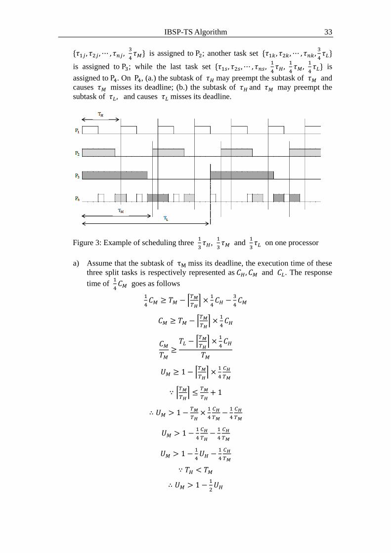
IBSP-TS Algorithm 33
is assigned to ; another task set
is assigned to ; while the last task set
is
assigned to . On , (a.) the subtask of may preempt the subtask of and
causes misses its deadline; (b.) the subtask of and may preempt the
subtask of and causes misses its deadline.
Figure 3: Example of scheduling three
,
and
on one processor
a) Assume that the subtask of miss its deadline, the execution time of these
three split tasks is respectively represented as and . The response
time of
goes as follows
34 IBSP-TS Algorithm
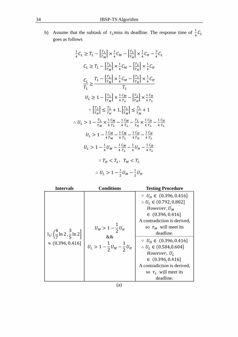
b) Assume that the subtask of miss its deadline. The response time of
goes as follows
,
Intervals Conditions Testing Procedure
&&
A contradiction is derived,
so will meet its
deadline.
A contradiction is derived,
so will meet its
deadline.
(a)

IBSP-TS Algorithm 35
Intervals Conditions Testing Procedure
&&
A contradiction is derived,
so will meet its
deadline.
A contradiction is derived,
so will meet its
deadline.
(b)
Table 3: Non-parallel execution proof for three split tasks
From Table 3, it is clear that
Thus, all the subtasks do not run simultaneously.
4.3 Phase Two
In Phase Two, all the residual tasks in along with those tasks from the last
interval constitute a task set called unassigned tasks. By using the idea of SPA2
algorithm, those unassigned tasks are assigned into the processors left after Phase
One.
4.3.1 Assignment Procedure
Lemma 2: A Unassigned task set with N tasks is schedulable on m processors
if [4].
The assignment procedure in SPA2 ensures the bound of ln2 in worst case. It contains
following steps:
1. Sort all the unassigned tasks in decreasing priority order.

36 IBSP-TS Algorithm
2. Define a task is a heavy task if its utilization
3. A heavy task is determined to be a pre-assigned to a single processor if the
following condition satisfies, is the number of unused processors left at
the time being.
These processors are called pre-assigned processors. All the rest processors are
called normal processors. The remaining tasks after pre-assignment step become
normal tasks.
4. Sort all the normal processors based on system utilization (the sum of utilization
of all the tasks have been assigned to a processor).
5. Assign a normal task to a normal processor whose utilization is minimal
among all normal processors.
6. If a normal task cannot be fully assigned to a normal processor Pnorm,
split and assign as much as possible to Pnorm. Now Pnorm is fully utilized which
means its utilization equals to . The rest split part of becomes a new
normal task and put back in the unassigned normal task queue.
7. Go to Step 4 until all normal processors are fully utilized.
8. Sort all the pre-assigned processors in increasing priority order.
9. Assign as many normal tasks as possible to a pre-assigned processor Ppre until it
is fully utilized. Then select next pre-assigned processor.
10. If a normal task cannot be fully assigned to Ppre, assign the split part to the next
selected pre-assigned processor.
4.3.2 Non-Parallel Execution
Proposition 2: No subtasks in Phase Two suffers from parallel execution problem.
SPA2 has already proved that their algorithm do not suffer the problem of subtasks
running in parallel. There are some facts they have shown.
1. Each pre-assigned task has the lowest priority on its host processor.
2. Each body subtask (all the subtasks split from a normal task excluding the last
split part) has the highest priority on its host processor.

IBSP-TS Algorithm 37
4.4 Utilization Bound
Theorem: If a task set has utilization , all the tasks can be scheduled
in m processors.
Proof: Let U1 be the utilization of the tasks which have been assigned in Phase One.
Denote m1 as the number of processors used in Phase One. By Lemma 1, it is certain
that
Let U2 be the utilization of the tasks which have been assigned in Phase Two. There
must exist some integer x such that
According to Lemma 2, all the unassigned tasks in Phase Two can be scheduled on
x+1 processors if .
4.5 Pseudo Code
There are some notifications for the algorithm shown in Figure 4:
is the utilization of a task and is the utilization of a processor.
represents the set of tasks belonging to different intervals
and is the assignment policy for .
means the set of residual tasks in after applying ;
and UnassignQ is the queue for unassigned tasks sorted in decreasing priority
order.

38 IBSP-TS Algorithm
is the count number of how many processors left after applying all the
policies.
and the sets represent processors contains pre-assigned tasks and
processors with no pre-assigned tasks respectively. is sorted in increasing
order of its pre-assigned tasks priority.
NormQ is the list of unassigned tasks after pre-assignment step, initial to be
empty.
1.
2.
3.
4.
5.
6.
7.
8.
9.
10.
11.
12.
13.
14.
15.
16.
17.
18.
19.
20.
21.
22.
23.
24.
25.
26.
27.
28.
29.
30.
31.
32.
33.
34.

IBSP-TS Algorithm 39
35.
36.
37.
38.
39.
40.
41.
42.
Figure 4: Pseudo code of IBSP-TS
1. Line 1~5: Assign a task to an interval list based on the utilization of the task.
2. Line 6~9: Apply tasks in each interval with a different policy. Put all the
unassigned first 26 intervals together with tasks in last interval into the
unassigned task queue.
3. Line 10: If the number of processors left after Phase One (all 26 policies) is less
or equal to 0, assignment failed.
4. Line 11: Sort all the tasks in the unassigned queue in decreasing priority order.
5. Line 12~20: Determine whether a unassigned task is a pre-assigned task or a
normal task. If the condition is satisfied, the task is a pre-assigned task. Assign
the task into a processor namely the pre-assigned processor. If the condition is not
satisfied, put the task into a queue called normal task queue. All the left
processors other than pre-assigned processors are called normal processors.
6. Line 21: Sort the index of pre-assigned processors in increasing priority order in
term of the pre-assigned tasks on those processors.
7. Line 22~42: If there is a normal task unassigned, try to assign it to a normal
processor first which has the minimal utilization among all normal processor. If it
cannot be fully assigned to a normal processor, split the task and assign a subtask
which can exactly make the normal processor fully utilized. If all normal
processors are fully utilized, assign the task to a pre-assigned processor which is
sorted in increasing priority order based on the pre-assigned task on that
processor. If the task is assigned and the pre-assigned processor is not fully
utilized, put the pre-assigned processor back to the list with its original index. If a
task cannot be fully assigned to a pre-assigned processor, split the task and assign
a subtask which can exactly make the pre-assigned processor fully utilized.
4.6 An Assignment Example
Here, an example of how a task is assigned by IBSP-TS is given in order to give a

40 IBSP-TS Algorithm
better understand of the algorithm.
12 tasks in a task set are going to be assigned on 8 processors
. The utilization range of these tasks is (0, 1] and the periods of the
tasks are randomly generated within 0 and 1000 time unit.
All the 12 tasks are listed as follows. Ui and Ti are the utilization, period of the task; In
is the interval which the task belongs to. Table 4 shows the 12 tasks in the task set.
I2 U1=0.652583 T1=550
I23 U2=0.113183 T2=528
I2 U3=0.578995 T3=508
I3 U4=0.485351 T4=89
I27 U5=0.038732 T5=235
I1 U6=0.976029 T6=720
I6 U7=0.372674 T7= 671
I1 U8=0.823314 T8=210
I7 U9=0.317253 T9=941
I3 U10=0.477383 T10=221
I1 U11=0.743396 T11=838
I3 U12=0.463743 T12=110
Table 4: Example of a task set
In Phase One, and are assigned to three dedicated processors, P1, P2 and
P3. According to Policy I3, the highest priority task in I3, is picked and equally split
into and
. along with are assigned to P4;
and together are
assigned to P5. Table 5 is the processors assigned in Phase One.
P1
P2
P3
(a)
P4
P5
(b)
Table 5: The assignment in Phase One
After Phase One, only three processor P6 , P7 and P8 are left. Since there are 6 tasks
left, . All the remaining unassigned tasks are sorted in decreasing
priority order. UnassignQ

IBSP-TS Algorithm 41
According to the condition, is a pre-assigned task if
,
Pre-assigned tasks are PreQ sorted in increasing priority order. Normal tasks
are NormQ .
Assign the first two pre-assign tasks and in two processors, P6 and P7.
Thereafter, normal tasks are assigned. Firstly, assign the to the left processor P8.
Since there is only one normal processor, the minimal utilization processor picked in
next assignment is still P8 until it becomes fully utilized. Therefore, and
are directly assigned to P8. However, the processor utilization do not allow to be
fully assigned to P8. It split into two parts, and
so that can be
assigned to P8 and make P8 precisely fully utilized. Next, the scheduling dispatcher
picks the first pre-assigned processor to assign the rest part of . It select P6 and try
to assign as much as possible, but still cannot be fully assigned into P6. Then,
is again split into two parts and
so that can be assigned to P6 and fully
utilize P6.Finally, the last part of , can be assigned to P7 and named as
.
Table 6 is the processors assigned in Phase Two.
P8
Ui 0.038732 0.113183 0.372674 0.210182
Uti of P8 0.038732 0.151916 0.524590 0.734772
(a)
P6
Ui 0.652583 0.082189
Uti of P6 0.652583 0.734772
(b)
P7
Ui 0.578995 0.024881
Uti of P7 0.578995 0.603877
(c)
Table 7: The assignment in Phase Two

42 IBSP-TS Algorithm

43
V
Evaluation
In this section, the simulation results are shown to evaluate the performance of
IBSP-TS, and compare it to the pure SPA2 algorithm. To the best of our knowledge,
SPA2 is the only one algorithm at this moment which has already proved the
utilization bound of 69.3% based on semi-partition fixed-priority scheduling. By
running the simulation, it shows that IBSP-TS performs much better than the SPA2
algorithms in most cases.
5.1 Simulation Setup
In all the simulations, there is a set of three parameters: Umin, Umax and m. The value m
means the number of processors in the system. The utilization of a randomly
generated task uniformly distributed within (Umin, Umax].
There are six sets of parameter m, the number of processors, in the simulation, which
are m=4, m=8, m=16, m=32, m=64 and m=128. This parameter m is used to estimate
the impact of increasing number of processors and the schedulability. For the
utilization range, (Umin, Umax], there are five sets, (0, 1], (0, 0.25], (0, 0.5], (0.25, 0.75]
and (0.5, 1] to represent mixed, extra light, normal light, medium and heavy task
utilization respectively. Thus, it is easy to observe whether there is any impact
because of different individual task utilization. Therefore, totally there are
different parameter sets for simulation experiments.
For each parameter set, 1,000,000 task sets are generated. Each task set contains a
number of randomly generated tasks. A task set is said to be schedulable if all the
tasks in a task set can be successfully assigned to no more than the number of
processors provided in the system which is m. The 1,000,000 task sets are generated

44 Evaluation
according to the following procedure:
1. Initially, m+1 tasks are generated in the first task set.
2. Calculate whether the task set is an infeasible task set
3. If it is an infeasible task set, reset the number of tasks in a task set to m+1.
4. Verify whether this task set can be scheduled by either IBSP-TS or SPA2.
5. If the task set is schedulable by either of those two algorithms, then calculate the
necessary metrics ( e.g. count the number of total split tasks, number of sorted
tasks and maximum number of subtasks in a task) to evaluate the performance of
the experiment.
6. Increase the number of tasks in next task set by 1.
To evaluate the performance of an algorithm, several measures are needed in the
simulation.
For each experiment, the schedulability of an algorithm can be estimated by the term
of success ratio, which is defined as follows.
The greater value of success ratio an algorithm has the better performance of
schedulability the algorithm is. In addition, 100 buckets (scales) are set to represent
the system utilization of a task set which is from 0 to 100%. In each bucket, an
individual success ratio (for example, the success ratio for task set with system
utilization 69%) is calculated. Since both algorithms has theoretically proved the
schedulability bound for task sets with ln2, all the individual success ratio should be
100% if the system utilization is below 69% (excluding 69%). Bucket 69% can
contain utilization 69.9% which is greater than Ln2. Moreover, it is good for an
algorithm to have a higher Break-down Point (the individual success ratio becomes no
more 100%), which can actually extend the utilization bound in real cases.
Meanwhile, since in real situation, task migration cost is not negligible, it is better for
an algorithm to have as smaller number of single task being split and subtasks (split
tasks from a single task) as possible. Thus, average number of split tasks (Avg. Split),
the average number of sorted tasks (Avg. Sort) and the maximum number of subtasks
split from a single task (Max Sub) are also important properties for an algorithm.

Evaluation 45
However, due to many factors, one algorithm may have worse Success Ration but it
perform better schedulability in some cases. Another measure is defined, which is
called Superiority. It means that a task set can be schedulable by one algorithm, but
not schedulable by the other one.
The simulation code is shown in Appendix.
5.2 Simulation Result
The results of the thirty experiments for both algorithms are grouped into six
categories which are based on different sets for parameters (Umin, Umax]. The statistics
for every five different m is shown in tables and figures.
Table 7 gives the results of simulation for mixed tasks within (0, 1]. The difference of
success ratio between IBSP-TS and SPA2 increases along with the increment of
number of processors. It starts from around 6% to more than 18%. Moreover, there
are some critical advantages for IBSP-TS. The maximum number of subtasks for
IBSP-TS is always less or equal to that of SPA2. In the worst case for SPA2, it even
makes a task migrate 116 times. Additionally, the less average number of sorted tasks
in IBSP-TS is a great property for online scheduling, and this property is always the
same in all five groups of simulations. The reason why IBSP-TS has these advantages
is Phase One in IBSP-TS, when the number of tasks in each task set increases, the
chance of more tasks can be handled in different first 26 intervals is becoming bigger
and bigger. However, this will make IBSP-TS has more split tasks if there are more
processors available (m>8). Furthermore, the superiority of SPA2 only happens when
m is small, for example, m=4 or m=8, but for IBSP-TS, it can have 26% in best case.
IBSP-TS SPA2
1
IBSP-TS SPA2
Success Ratio 62.5893% 56.1998% Success Ratio 63.2001% 54.3822%
Avg. Split 0.2850 0.4477 Avg. Split 0.5233 0.5968
Avg. Sort 4.3916 5.7735 Avg. Sort 7.5195 10.6983
Max. Sub 4 4 Max. Sub 7 8
Superiority 10.2334% 0.0274% Superiority 13.9526% 0.0003%
(a) m=4 (b) m=8
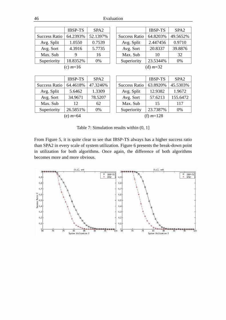
46 Evaluation
IBSP-TS SPA2
1
IBSP-TS SPA2
Success Ratio 64.2393% 52.1397% Success Ratio 64.8203% 49.5652%
Avg. Split 1.0550 0.7539 Avg. Split 2.447456 0.9710
Avg. Sort 4.3916 5.7735 Avg. Sort 20.8337 39.8876
Max. Sub 9 16 Max. Sub 10 32
Superiority 18.8352% 0% Superiority 23.5344% 0%
(c) m=16 (d) m=32
IBSP-TS SPA2
1
IBSP-TS SPA2
Success Ratio 64.4618% 47.3246% Success Ratio 63.8920% 45.5303%
Avg. Split 5.6462 1.3309 Avg. Split 12.9382 1.9672
Avg. Sort 34.9671 78.5207 Avg. Sort 57.6213 155.6472
Max. Sub 12 62 Max. Sub 15 117
Superiority 26.5851% 0% Superiority 23.7387% 0%
(e) m=64 (f) m=128
Table 7: Simulation results within (0, 1]
From Figure 5, it is quite clear to see that IBSP-TS always has a higher success ratio
than SPA2 in every scale of system utilization. Figure 6 presents the break-down point
in utilization for both algorithms. Once again, the difference of both algorithms
becomes more and more obvious.

Evaluation 47
Figure 5: Success ratio in simulations within (0, 1] with different m
Figure 6: Break-down point in simulations within (0, 1]
64
66
68
70
72
74
76
78
80
m=4 m=8 m=16 m=32 m=64 m=128
IBSP-TS
SPA2

48 Evaluation
Table 8 shows the results of simulation for extra light tasks within (0, 0.25]. The
difference of success ratio between two algorithms increases from 0.2% to 2% when
m increases. However, due to the light task (0, 0.25], there are less intervals used in
Phase One, which causes IBSP-TS becomes more or less as same as SPA2. Thus, the
Avg. Sort for IBSP-TS is quite close to that of SPA2. For Max. Sub, IBSP-TS may
suffer the same problem as SPA2 because of no pre-assigned tasks and the
assignments for last several very light tasks, but when m=128, IBSP-TS has 7 less
subtasks than SPA2. However, IBSP-TS still perform a bit better than SPA2 which is
listed by superiority, and even when m=4, the superiority of SPA2 is negligible.
IBSP-TS SPA2
1
IBSP-TS SPA2
Success Ratio 71.5340% 71.3367% Success Ratio 70.6056% 70.1482%
Avg. Split 0.1492 0.1701 Avg. Split 0.2696 0.3640
Avg. Sort 13.5280 13.786403 Avg. Sort 25.4879 26.8990
Max. Sub 4 4 Max. Sub 7 7
Superiority 0.2769% 0.0003% Superiority 0.6476% 0%
(a) m=4 (b) m=8
IBSP-TS SPA2
1
IBSP-TS SPA2
Success Ratio 69.9035% 69.0946% Success Ratio 69.6106% 68.2750%
Avg. Split 0.5105 0.7491 Avg. Split 1.2082 1.5135
Avg. Sort 47.5833 53.0866 Avg. Sort 86.0277 105.4322
Max. Sub 10 10 Max. Sub 11 15
Superiority 1.1572% 0% Superiority 1.9187% 0%
(c) m=16 (d) m=32
IBSP-TS SPA2
1
IBSP-TS SPA2
Success Ratio 69.3125% 67.5807% Success Ratio 68.9200% 66.8760%
Avg. Split 3.6731 3.0477 Avg. Split 10.4517 6.1051
Avg. Sort 148.6568 210.1630 Avg. Sort 252.4917 419.4665
Max. Sub 14 19 Max. Sub 13 22
Superiority 2.4985% 0% Superiority 2.9658% 0%
(e) m=64 (f) m=128
Table 8: Simulation results for tasks within (0, 0.25]
For extra light tasks, generally, both algorithms have more or less the same
performance. However, it is still the truth that IBSP-TS has higher success ratio and
break-down point as shown in Figure 7 and Figure 8.

Evaluation 49
Figure 7: Success ratio in simulations within (0, 0.25] with different m

50 Evaluation
Figure 8: Break-down point in simulations within (0, 0.25]
Table 9 shows the results of simulation for normal light tasks within (0, 0.5]. The
difference of success ratio between two algorithms rises from around 0.6% to 4% with
increment value m. Since it is still considered to be light tasks, in some cases, the
performance are similar for both algorithms. IBSP-TS is again better than SPA2 for
all the statistics. The superiority of SPA2 when m=4 is still too small to be noticed.
IBSP-TS SPA2
1
IBSP-TS SPA2
Success Ratio 67.9117% 67.3575% Success Ratio 67.0182% 65.9863%
Avg. Split 0.4683 0.5297 Avg. Split 0.9414 1.1221
Avg. Sort 7.8863 8.2655 Avg. Sort 14.4441 15.8448
Max. Sub 4 4 Max. Sub 8 8
Superiority 0.8180% 0.0002% Superiority 1.5397% 0%
(a) m=4 (b) m=8
IBSP-TS SPA2
1
IBSP-TS SPA2
Success Ratio 66.5590% 64.7012% Success Ratio 66.2644% 63.5591%
Avg. Split 1.8953 2.2901 Avg. Split 4.3302 4.5985
Avg. Sort 25.8697 30.9503 Avg. Sort 44.5071 61.1194
Max. Sub 10 12 Max. Sub 13 15
Superiority 2.7912% 0% Superiority 4.0826% 0%
(c) m=16 (d) m=32
64
66
68
70
72
74
76
78
80
m=4 m=8 m=16 m=32 m=64 m=128
IBSP-TS
SPA2

Evaluation 51
IBSP-TS SPA2
1
IBSP-TS SPA2
Success Ratio 66.0109% 62.5631% Success Ratio 65.7586% 61.8576%
Avg. Split 10.4161 9.2292 Avg. Split 25.2838 18.5089
Avg. Sort 72.9510 121.4573 Avg. Sort 166.2817 242.2193
Max. Sub 15 20 Max. Sub 19 27
Superiority 5.2231% 0% Superiority 5.9323% 0%
(e) m=64 (f) m=128
Table 9: Simulation results for tasks within (0, 0.5]
In Figure 9, the trend of success ratio is the same as previous observation for mixed
tasks and normal tasks. For the break-down point shown in Figure 10, IBSP-TS
dominates the other.

52 Evaluation
Figure 9: Success ratio in simulations within (0, 0.5] with different m
Figure 10: Break-down point in simulations within (0, 0.5]
Table 10 is the statistics of simulation for medium tasks within (0.25, 0.75]. The
difference of success ratio between two algorithms increases from around 3% to 17%.
Moreover, for superiority, IBSP-TS performs twice as good as SPA2 when m is
relatively big. This shows that IBSP-TS is better for higher utilization tasks. It is
because in IBSP-TS, the idea of a part of the algorithm is from SPA2, thus, it makes
IBSP suffer the same problem as SPA2 when all the tasks are light. The price of
higher success ratio and superiority is a more split tasks. However, considered the
great improvement of IBSP-TS, it is acceptable.
64
66
68
70
72
74
76
78
80
m=4 m=8 m=16 m=32 m=64 m=128
IBSP-TS
SPA2

Evaluation 53
IBSP-TS SPA2
1
IBSP-TS SPA2
Success Ratio 12.9744% 9.3209% Success Ratio 28.5884% 17.6567%
Avg. Split 1.0005 1.0000 Avg. Split 1.3275 1.0172
Avg. Sort 2.7858 5.0000 Avg. Sort 2.5347 9.0169
Max. Sub 4 4 Max. Sub 5 8
Superiority 28.3906% 0.3219% Superiority 38.2382% 0%
(a) m=4 (b) m=8
IBSP-TS SPA2
1
IBSP-TS SPA2
Success Ratio 33.2281% 17.7830% Success Ratio 35.5960% 18.0860%
Avg. Split 2.7815 1.4055 Avg. Split 5.9868 2.2608
Avg. Sort 2.8645 17.4052 Avg. Sort 2.9442 34.2604
Max. Sub 5 16 Max. Sub 5 30
Superiority 46.4820% 0% Superiority 49.1909% 0%
(c) m=16 (d) m=32
IBSP-TS SPA2
1
IBSP-TS SPA2
Success Ratio 36.7294% 18.2315% Success Ratio 37.3115% 18.2986%
Avg. Split 12.4927 3.9909 Avg. Split 25.5589 7.4895
Avg. Sort 2.9792 67.9989 Avg. Sort 2.9906 135.4894
Max. Sub 5 36 Max. Sub 5 37
Superiority 50.3627% 0% Superiority 50.9572% 0%
(e) m=64 (f) m=128
Table 10: Simulation results for tasks within (0.25, 0.75]
Figure 11 and Figure 12 are the graphs for success ratio and break-down point.

54 Evaluation
Figure 11: Success ratio in simulations within (0.25, 0.75] with different m
Figure 12: Break-down point in simulations within (0.25, 0.75]
64
66
68
70
72
74
76
78
80
m=4 m=8 m=16 m=32 m=64 m=128
IBSP-TS
SPA2

Evaluation 55
Table 11 presents the simulation results for heavy tasks within (5, 1]. Because of high
utilization of each individual tasks, the success ratio for both algorithms is quite low.
SPA2 can barely schedule the task sets, which leads the superiority of IBSP-TS to
more than 90% and even close to 100%. This fully shows the bad performance of
SPA2 when it deals with high utilization task sets. In both average sorted tasks and
maximum subtasks, IBSP-TS has huge advantage over SPA2 when m are relatively
large.
IBSP-TS SPA2
1
IBSP-TS SPA2
Success Ratio 2.5584% 0.9197% Success Ratio 10.9078% 0.9402%
Avg. Split 1.0001 1.0000 Avg. Split 1.0203 1.0257
Avg. Sort 2.1216 5.0000 Avg. Sort 2.5347 9.0169
Max. Sub 4 4 Max. Sub 5 8
Superiority 64.0896% 0.1054% Superiority 91.3805% 0%
(a) m=4 (b) m=8
IBSP-TS SPA2
1
IBSP-TS SPA2
Success Ratio 22.1257% 0.6156% Success Ratio 27.1188% 0.2832%
Avg. Split 1.3598 1.1556 Avg. Split 2.6948 1.5448
Avg. Sort 2.6832 17.0101 Avg. Sort 2.8902 33.0230
Max. Sub 5 16 Max. Sub 5 32
Superiority 97.2177% 0% Superiority 98.9557% 0%
(c) m=16 (d) m=32
IBSP-TS SPA2
1
IBSP-TS SPA2
Success Ratio 29.3367% 0.1099% Success Ratio 30.3594% 0.0395%
Avg. Split 5.6993 2.5960 Avg. Split 11.8472 5.1089
Avg. Sort 2.9517 65.0246 Avg. Sort 2.9788 129.0203
Max. Sub 5 62 Max. Sub 5 52
Superiority 99.6254% 0% Superiority 99.8699% 0%
(e) m=64 (f) m=128
Table 11: Simulation results for tasks within (0.25, 0.75]
Figure 13 and Figure 14 shows the success ratio and break-down point for both
algorithms.

56 Evaluation
Figure 13: Success ratio in simulations within (0.5, 1] with different m

Evaluation 57
Figure 14: Break-down point in simulations within (0.5, 1]
64
66
68
70
72
74
76
78
80
m=4 m=8 m=16 m=32 m=64 m=128
IBSP-TS
SPA2

58 Evaluation

59
VI
Conclusion
The research in this thesis is to design a static-priority scheduling algorithm in a
multi-processor real-time system which can assign a set of independent periodic tasks
to a number of processors in the system and ensure each task does not miss its
deadline. Therefore, the IBSP-TS (Interval Based Semi-Partitioned Task Splitting)
algorithm is derived. It combines the idea of the IBPS algorithm and the SPA
algorithm with semi-partition technique and RM priority policy to achieve the highest
possible worst-case utilization bound to ln2.
Note: there are some assumptions in IBSP-TS for systems and tasks. The
multi-processor system used for IBSP-TS assumes that all the processors are identical
and data-shareable; also there is no task migration do not have cost. Moreover, tasks
are independent and preemptive. There is no synchronization among tasks. No jobs of
a task or subtasks can be executed on two or more processors simultaneously, and a
processor cannot execute two or more tasks simultaneously
The schedulability test of IBSP is divided into two parts together with the assignment
procedure. In Phase One, by calculating the worst-case processor work load within
each interval, the Hyperbolic Bound test can guarantee the feasibility. In Phase Two,
the Liu & Layland test ensure the assignment procedure only schedule a feasible
number of tasks on a processor. Therefore, if ln2 which is 69.3% capacity of
processors in a system is used, all the tasks in the task set can meet their deadlines.
Although IBSP-TS has the same worst-case utilization bound of SPA, it has some
advantages over SPA2. First of all, there are less sorted tasks in the assignment, which
is suitable for online scheduling for multi-processor system. Certainly, the sorting
itself is also time consuming. Besides, IBSP-TS leaves the algorithm implementation
decision to the system designers. They can come up with their preferred choice by
selecting the number of intervals in the system implementation. The more intervals,

60 Conclusion
the less number of sorted tasks there are.
From simulation, IBSP-TS also shows its superiority to SPA2. In most cases, if a task
can be scheduled by SPA2, it can be scheduled by IBSP-TS as well. However, only
when the number of processors in the system is quite small, there may be few task
sets which are only schedulable by SPA2. Nevertheless, in terms of task sets success
ratio, average number of split tasks and maximum number of subtasks, IBSP-TS is
much better than SPA2 in general utilization tasks or heavy utilization tasks. The
lower number of task migrations, the less preemption cost there is. Additionally, the
break-down point in utilization for IBSP-TS can reach to 76% for general tasks; and
for heavy tasks, it can be 79%.
In summary, IBSP-TS provides a feasibility condition with the highest possible
worst-case utilization bound condition as ln2, less task migrations and higher success
ratio compared to the best static-priority multi-processor scheduling at this time being.
Moreover, IBSP-TS can adopt other priority polices as well, for example
deadline-monotonic. Additionally, it leaves the implementation decision in IBSP-TS
to system designers. All these properties make IBSP-TS more efficiently to schedule
tasks in multi-processor real-time systems compared to many other competing
scheduling algorithms.

61
Bibliography
[1] “Tilera Targets Intel, AMD With 100-core Processor” PCWorld. Oct 26 2009. May
20 2010.
<http://www.pcworld.com/article/174318/tilera_targets_intel_amd_with_100core_pr
ocessor.html>
[2] B. Andersson and J. Jonsson. The Utilization Bounds of Partitioned and Pfair
Static-Priority Scheduling on Multi-processors are 50%. In Proceedings of the
Euromicro Conference on Real-Time Systems, pages 33–40, 2003.
[3] R. M. Pathan and J. Jonsson. Load Regulating Algorithm for Static-Priority Task
Scheduling on Multiprocessors. In Proceedings of 24th IEEE International Parallel
and Distributed Processing Symposium, 2010.
[4] Nan Guan, Martin Stigge, Wang Yi and Ge Yu. Fixed-Priority Multiprocessor
Scheduling with Liu & Layland’s Utilization Bound.
[5] C. L. Liu and J.W. Layland. Scheduling Algorithms for Multiprogramming in a
Hard Real-Time Environment. Journal of the ACM, 20:46–61, 1973.
[6] Enrico Bini, Giorgio C. Buttazzo, Member, IEEE, and Giuseppe M. Buttazzo.
Rate Monotonic Analysis: The Hyperbolic Bound. IEEE Transactions on Computers,
VOL. 52, NO. 7, JULY 2003.
[7] L. Sha, J. P. Lehoczky, and R. Rajkumar. Solutions for Some Practical problems
in Prioritized Preemptive Scheduling. In Proceedings of the IEEE Real-Time Systems
Symposium, pages 181–191, 1986.
[8] J. Lehoczky, L. Sha, and Y. Ding. The rate monotonic scheduling algorithm: exact

62 Bibliography
characterization and average case behavior. In Proceedings of the IEEE Real-Time
Systems Symposium, pages 166–171, 1989.
[9] L. Sha, R. Rajkumar, and J.P. Lehoczky. Priority Inheritance Protocols: An
Approach to Real-Time Synchronization. IEEE Transactions on Computers,
39(9):1175–1185, 1990.
[10] S. Baruah, N. Cohen, C.G. Plaxton, and D. Varvel. Proportionate Progress: A
Notion of Fairness in Resource Allocation. Algorithmica, 15:600–625, 1996.
[11] S. Baruah, J. Gehrke, and C.G. Plaxton. Fast Scheduling of Periodic Tasks on
Multiple Resources. In Proceedings of the International Parallel Processing
Symposium, pages 280–288, 1995.
[12]B. Andersson and E. Tovar. Multiprocessor Scheduling with Few Preemptions. In
Proceedings of the IEEE International Conference on Embedded and Real-Time
Computing Systems and Applications, pages 322–334, 2006.
[13] H. Cho, B. Ravindran, and E. D. Jensen. An Optimal Real-Time Scheduling
Algorithm for Multiprocessors. In Proceedings of the IEEE Real-Time Systems
Symposium, pages 101–110, 2006.
[14] J. Goosens, S. Funk, and S. Baruah. Priority-Driven Scheduling of Periodic Task
Systems on Multiprocessors. Real-Time Systems, 25:187–205, 2003.
[15] T. P. Baker. An Analysis of EDF Schedulability on a Multiprocessor. IEEE Trans.
on Parallel and Distributed Systems, 16:760–768, 2005.
[16] M. Cirinei and T.P. Baker. EDZL Scheduling Analysis. In Proceedings of the
Euromicro Conference on Real-Time Systems, pages 9–18, 2007.
[17] S. Dhall and C. Liu: On a real-time scheduling problem. Operations Research,
vol. 6, pages 127-140, 1978.
[18] B. Andersson, S. Baruah, J.Jonsson. Static-Prioriy Scheduling on
Multiprocessors. In Proceedings of IEEE Real-Time Systems Symposium, London, UK,
2001.
[19] L. Lundberg. Analyzing Fixed-Priority Global Multiprocessor Scheduling. In
Proceedings of Eighth IEEE Real-Time and Embedded Technology and Applications
Symposium, 2002.
[20] B. Andersson. Global static priority preemptive multiprocessor scheduling with
utilization bound 38%. In OPODIS, 2008.
[21] S. Ramamurthy. Scheduling Periodic Hard Real-Time Tasks with Arbitrary
Deadlines on Multiprocessors. In Proceedings of the IEEE Real-Time systems
Symposium, pages 59-68, 2002.

Bibliography 63
[22] S. K. Dhall and C. L. Liu. On a Real-Time Scheduling Problem. Operations
Research, 26:127-140,1978.
[23] D.-I. Oh and T. P. Baker. Utilization Bounds for N-Processor Rate Monotone
Scheduling with Static Processor Assignment. Real-Time Systems, 15(2):183–192,
1998.
[24] Y. Oh and S. Son. Allocating Fixed-Priority Periodic Tasks on Multiprocessor
Systems. Real-Time Systems, 9:207-239, 1995.
[25] S. Lauzac, R. Melhem, and D. Moss e. An efficient RMS admission control and
its application to multiprocessor scheduling. In Proceedings of the IEEE International
Parallel Processing Symposium, pages 511–518, Orlando, Florida, March 1998.
[26] J. M. Lopez, J. L. Diaz, and D. F. Garcia. Utlization Bounds for EDF Scheduling
on Real-Time Multiprocessor Systems. Real-Time Systems, 28:39–68, 2004.
[27] S. Kato and N. Yamasaki. Portioned static-priority scheduling on multiprocessors.
In Proceedings of IEEE International Parallel and Distributed Processing Symposium.
IPDPS, 2008, pages 1 – 12.
[28] S. Kato and N. Yamasaki. Semi-partitioned fixed-priority scheduling on
multiprocessors. In Proceedings of 15th IEEE Real-Time and Embedded Technology
and Applications Symposium, 2009. RTAS 2009, pages 23 – 32.
[29] K. Lakshmanan, R. Rajkumar and J. Lehoczky. Partitioned Fixed-Priority
Preemptive Scheduling for Multi-core Processors. In Proceedings of the 21st
Euromicro Conference on Real-Time Systems, 2009, pages 239 – 248, 2009.
[30] S. Kato and N. Yamasaki. Real-Time Scheduling with Task Splitting on
Multiprocessors. In Proceedings of the 13th IEEE International Conference on
Embedded and Real-Time Computing Systems and Applications, pages 441-450, 2007.
[31] S. Kato and N. Yamasaki. Portioned EDF-based Scheduling on multiprocessors.
In Proceedings of the 8th ACM/IEEE International Conference on Embedded
Software, pages 139-148, 2008.
[32] S. Kato and N. Yamasaki. Semi-Partitioning Technique for Multiprocessor
Real-Time Scheduling. In the 29th IEEE Real-Time Systems Symposium, 2008.


65
Appendix
The simulation C code for the performance comparison between IBSP-TS and SPA is
attached as follows.
#include<stdio.h>
#include<stdlib.h>
#include<time.h>
#include<math.h>
#include<malloc.h>
#define SET 1000000
#define PROC 128
#define N 1
#define Ln logl(2)
typedef struct{
double uti;
int period;
} task;
int task_num=PROC+N;
double weight, theta;
task arr_task[PROC*10];
double tot_uti;
int chaox_split;
int chaox_sub;
int chaox_sort;
int neu_split;

66 Appendix
int neu_sub;
int neu_sort;
int chaox_return;
int neu_return;
double init()
{
int i;
double tmp;
tot_uti=0;
for(i=0;i<task_num;i++){
tmp=rand();
if(tmp==0)
tmp=rand();
arr_task[i].uti=tmp/(4.0*RAND_MAX);
tot_uti=tot_uti+arr_task[i].uti;
}
while(tot_uti>PROC){
task_num=PROC+N;
printf("Regenerate & task_num %d\n", task_num);
tot_uti=0;
for(i=0;i<task_num;i++){
tmp=rand();
if(tmp==0)
tmp=rand();
arr_task[i].uti=tmp/(4.0*RAND_MAX);
tot_uti=tot_uti+arr_task[i].uti;
}
}
for(i=0;i<task_num;i++){
arr_task[i].period=rand()%1000;
//printf("period %d\n", arr_task[i].period);
//printf("uti %f\n", arr_task[i].uti);
}
theta=(pow(2,(1.0/task_num))-1)*task_num;
weight=theta/(theta+1);
printf("task_num %d theta %f weight %f\n",task_num, theta, weight);
}
double chaox()
{
int i, j, x, m, n, p, k, t, flg, proc_num, count_x;
double x_uti, tmp, new_weight, new_theta, c;
int *subtask;

Appendix 67
double *uti, *pre_cpu, *norm_cpu;
int count_1, count_2, count_3, count_4, count_5, count_6, count_7, count_8,
count_9, count_10, count_11, count_12, count_13, count_14, count_15, count_16,
count_17, count_18, count_19, count_20, count_21, count_22, count_23, count_24,
count_25, count_26, count_27, count_pre, count_norm;
task *a2, *a3, *a4, *a5, *a6, *a7, *a8, *a9, *a10, *a11, *a12, *a13, *a14, *a15,
*a16, *a17, *a18, *a19, *a20, *a21, *a22, *a23, *a24, *a25, *a26, *ax, *pre, *norm;
int rem_2, rem_3, rem_4, rem_5, rem_6, rem_7, rem_8, rem_9, rem_10,
rem_11, rem_12, rem_13, rem_14, rem_15, rem_16, rem_17, rem_18, rem_19,
rem_20, rem_21, rem_22, rem_23, rem_24, rem_25, rem_26, rem_x;
count_1=0;
count_2=0;
count_3=0;
count_4=0;
count_5=0;
count_6=0;
count_7=0;
count_8=0;
count_9=0;
count_10=0;
count_11=0;
count_12=0;
count_13=0;
count_14=0;
count_15=0;
count_16=0;
count_17=0;
count_18=0;
count_19=0;
count_20=0;
count_21=0;
count_22=0;
count_23=0;
count_24=0;
count_25=0;
count_26=0;
count_27=0;
chaox_return=0;
for(i=0;i<task_num;i++){
if(arr_task[i].uti>Ln) count_1++;
else if(arr_task[i].uti<=Ln && arr_task[i].uti>(4.0/5*Ln)) count_2++;

68 Appendix
else if(arr_task[i].uti<=(4.0/5*Ln) && arr_task[i].uti>(2.0/3*Ln)) count_3++;
else if(arr_task[i].uti<=(2.0/3*Ln) && arr_task[i].uti>(3.0/5*Ln)) count_4++;
else if(arr_task[i].uti<=(3.0/5*Ln) && arr_task[i].uti>(4.0/7*Ln)) count_5++;
else if(arr_task[i].uti<=(4.0/7*Ln) && arr_task[i].uti>(1.0/2*Ln)) count_6++;
else if(arr_task[i].uti<=(1.0/2*Ln) && arr_task[i].uti>(4.0/9*Ln)) count_7++;
else if(arr_task[i].uti<=(4.0/9*Ln) && arr_task[i].uti>(2.0/5*Ln)) count_8++;
else if(arr_task[i].uti<=(2.0/5*Ln) && arr_task[i].uti>(4.0/11*Ln)) count_9++;
else if(arr_task[i].uti<=(4.0/11*Ln) && arr_task[i].uti>(1.0/3*Ln))
count_10++;
else if(arr_task[i].uti<=(1.0/3*Ln) && arr_task[i].uti>(4.0/13*Ln))
count_11++;
else if(arr_task[i].uti<=(4.0/13*Ln) && arr_task[i].uti>(2.0/7*Ln))
count_12++;
else if(arr_task[i].uti<=(2.0/7*Ln) && arr_task[i].uti>(3.0/11*Ln))
count_13++;
else if(arr_task[i].uti<=(3.0/11*Ln) && arr_task[i].uti>(1.0/4*Ln))
count_14++;
else if(arr_task[i].uti<=(1.0/4*Ln) && arr_task[i].uti>(4.0/17*Ln))
count_15++;
else if(arr_task[i].uti<=(4.0/17*Ln) && arr_task[i].uti>(2.0/9*Ln))
count_16++;
else if(arr_task[i].uti<=(2.0/9*Ln) && arr_task[i].uti>(3.0/14*Ln))
count_17++;
else if(arr_task[i].uti<=(3.0/14*Ln) && arr_task[i].uti>(1.0/5*Ln))
count_18++;
else if(arr_task[i].uti<=(1.0/5*Ln) && arr_task[i].uti>(4.0/21*Ln))
count_19++;
else if(arr_task[i].uti<=(4.0/21*Ln) && arr_task[i].uti>(2.0/11*Ln))
count_20++;
else if(arr_task[i].uti<=(2.0/11*Ln) && arr_task[i].uti>(3.0/17*Ln))
count_21++;
else if(arr_task[i].uti<=(3.0/17*Ln) && arr_task[i].uti>(1.0/6*Ln))
count_22++;
else if(arr_task[i].uti<=(1.0/6*Ln) && arr_task[i].uti>(4.0/25*Ln))
count_23++;
else if(arr_task[i].uti<=(4.0/25*Ln) && arr_task[i].uti>(2.0/13*Ln))
count_24++;
else if(arr_task[i].uti<=(2.0/13*Ln) && arr_task[i].uti>(3.0/20*Ln))
count_25++;
else if(arr_task[i].uti<=(3.0/20*Ln) && arr_task[i].uti>(1.0/7*Ln))
count_26++;
else count_27++;
}

Appendix 69
rem_2=count_2%5;
rem_3=count_3%3;
rem_4=count_4%5;
rem_5=count_5%7;
rem_6=count_6%2;
rem_7=count_7%9;
rem_8=count_8%5;
rem_9=count_9%11;
rem_10=count_10%3;
rem_11=count_11%13;
rem_12=count_12%7;
rem_13=count_13%11;
rem_14=count_14%4;
rem_15=count_15%17;
rem_16=count_16%9;
rem_17=count_17%14;
rem_18=count_18%5;
rem_19=count_19%21;
rem_20=count_20%11;
rem_21=count_21%17;
rem_22=count_22%6;
rem_23=count_23%25;
rem_24=count_24%13;
rem_25=count_25%20;
rem_26=count_26%7;
if(count_2 || count_5 || count_7 || count_9 || count_11 || count_15 ||
count_19 || count_23)
chaox_sub=4;
else if(count_4 || count_13 || count_17 || count_21 || count_25)
chaox_sub=3;
else if(count_3 || count_8 || count_12 || count_16 || count_20 || count_24)
chaox_sub=2;
else chaox_sub=0;
chaox_split=count_2/5+count_3/3+count_4/5*2+count_5/7*3+count_7/9+coun
t_8/5+count_9/11*3+count_11/13+count_12/7+count_13/11*2+count_15/17+coun
t_16/9+count_17/14*2+count_19/21+count_20/11+count_21/17*2+count_23/25+c
ount_24/13+count_25/20*2;
count_x=rem_2+rem_3+rem_4+rem_5+rem_6+rem_7+rem_8+rem_9+rem_10+
rem_11+rem_12+rem_13+rem_14+rem_15+rem_16+rem_17+rem_18+rem_19+rem
_20+rem_21+rem_22+rem_23+rem_24+rem_25+rem_26+count_27;
chaox_sort=count_x;

70 Appendix
x=count_x;
new_theta=(pow(2,(1.0/x))-1)*x;
new_weight=new_theta/(new_theta+1);
printf("new_theta %f new_weight %f\n", new_theta, new_weight);
proc_num=PROC-count_1-count_2/5*4-count_3/3*2-count_4/5*3-count_5/7*4
-count_6/2-count_7/9*4-count_8/5*2-count_9/11*4-count_10/3-count_11/13*4-co
unt_12/7*2-count_13/11*3-count_14/4-count_15/17*4-count_16/9*2-count_17/14
*3-count_18/5-count_19/21*4-count_20/11*2-count_21/17*3-count_22/6-count_2
3/25*4-count_24/13*2-count_25/20*3-count_26/7;
printf("proc_num %d\n", proc_num);
if(proc_num>0 && x>0){
a2=(task*)malloc(count_2*sizeof(task));
a3=(task*)malloc(count_3*sizeof(task));
a4=(task*)malloc(count_4*sizeof(task));
a5=(task*)malloc(count_5*sizeof(task));
a6=(task*)malloc(count_6*sizeof(task));
a7=(task*)malloc(count_7*sizeof(task));
a8=(task*)malloc(count_8*sizeof(task));
a9=(task*)malloc(count_9*sizeof(task));
a10=(task*)malloc(count_10*sizeof(task));
a11=(task*)malloc(count_11*sizeof(task));
a12=(task*)malloc(count_12*sizeof(task));
a13=(task*)malloc(count_13*sizeof(task));
a14=(task*)malloc(count_14*sizeof(task));
a15=(task*)malloc(count_15*sizeof(task));
a16=(task*)malloc(count_16*sizeof(task));
a17=(task*)malloc(count_17*sizeof(task));
a18=(task*)malloc(count_18*sizeof(task));
a19=(task*)malloc(count_19*sizeof(task));
a20=(task*)malloc(count_20*sizeof(task));
a21=(task*)malloc(count_21*sizeof(task));
a22=(task*)malloc(count_22*sizeof(task));
a23=(task*)malloc(count_23*sizeof(task));
a24=(task*)malloc(count_24*sizeof(task));
a25=(task*)malloc(count_25*sizeof(task));
a26=(task*)malloc(count_26*sizeof(task));
ax=(task*)malloc(count_x*sizeof(task));
for(i=0;i<task_num;i++){
if(arr_task[i].uti>Ln) continue;
else if(arr_task[i].uti<=Ln && arr_task[i].uti>(4.0/5*Ln)){
a2[count_2-1].uti=arr_task[i].uti;

Appendix 71
a2[count_2-1].period=arr_task[i].period;
//printf("a2 %f\n", a2[count_2-1]);
count_2--;
}
else if(arr_task[i].uti<=(4.0/5*Ln) && arr_task[i].uti>(2.0/3*Ln)){
a3[count_3-1].uti=arr_task[i].uti;
a3[count_3-1].period=arr_task[i].period;
//printf("a3 %f\n", a3[count_3-1]);
count_3--;
}
else if(arr_task[i].uti<=(2.0/3*Ln) && arr_task[i].uti>(3.0/5*Ln)){
a4[count_4-1].uti=arr_task[i].uti;
a4[count_4-1].period=arr_task[i].period;
//printf("a4 %f\n", a4[count_4-1]);
count_4--;
}
else if(arr_task[i].uti<=(3.0/5*Ln) && arr_task[i].uti>(4.0/7*Ln)){
a5[count_5-1].uti=arr_task[i].uti;
a5[count_5-1].period=arr_task[i].period;
//printf("a5 %f\n", a5[count_5-1]);
count_5--;
}
else if(arr_task[i].uti<=(4.0/7*Ln) && arr_task[i].uti>(1.0/2*Ln)){
a6[count_6-1].uti=arr_task[i].uti;
a6[count_6-1].period=arr_task[i].period;
//printf("a6 %f\n", a6[count_6-1]);
count_6--;
}
else if(arr_task[i].uti<=(1.0/2*Ln) && arr_task[i].uti>(4.0/9*Ln)){
a7[count_7-1].uti=arr_task[i].uti;
a7[count_7-1].period=arr_task[i].period;
//printf("a7 %f\n", a7[count_7-1]);
count_7--;
}
else if(arr_task[i].uti<=(4.0/9*Ln) && arr_task[i].uti>(2.0/5*Ln)){
a8[count_8-1].uti=arr_task[i].uti;
a8[count_8-1].period=arr_task[i].period;
//printf("a8 %f\n", a8[count_8-1]);
count_8--;
}
else if(arr_task[i].uti<=(2.0/5*Ln) && arr_task[i].uti>(4.0/11*Ln)){
a9[count_9-1].uti=arr_task[i].uti;
a9[count_9-1].period=arr_task[i].period;
//printf("a9 %f\n", a9[count_9-1]);

72 Appendix
count_9--;
}
else if(arr_task[i].uti<=(4.0/11*Ln) && arr_task[i].uti>(1.0/3*Ln)){
a10[count_10-1].uti=arr_task[i].uti;
a10[count_10-1].period=arr_task[i].period;
//printf("a10 %f\n", a10[count_10-1]);
count_10--;
}
else if(arr_task[i].uti<=(1.0/3*Ln) && arr_task[i].uti>(4.0/13*Ln)){
a11[count_11-1].uti=arr_task[i].uti;
a11[count_11-1].period=arr_task[i].period;
//printf("a11 %f\n", a11[count_11-1]);
count_11--;
}
else if(arr_task[i].uti<=(4.0/13*Ln) && arr_task[i].uti>(2.0/7*Ln)){
a12[count_12-1].uti=arr_task[i].uti;
a12[count_12-1].period=arr_task[i].period;
//printf("a12 %f\n", a12[count_12-1]);
count_12--;
}
else if(arr_task[i].uti<=(2.0/7*Ln) && arr_task[i].uti>(3.0/11*Ln)){
a13[count_13-1].uti=arr_task[i].uti;
a13[count_13-1].period=arr_task[i].period;
//printf("a13 %f\n", a13[count_13-1]);
count_13--;
}
else if(arr_task[i].uti<=(3.0/11*Ln) && arr_task[i].uti>(1.0/4*Ln)){
a14[count_14-1].uti=arr_task[i].uti;
a14[count_14-1].period=arr_task[i].period;
//printf("a14 %f\n", a14[count_14-1]);
count_14--;
}
else if(arr_task[i].uti<=(1.0/4*Ln) && arr_task[i].uti>(4.0/17*Ln)){
a15[count_15-1].uti=arr_task[i].uti;
a15[count_15-1].period=arr_task[i].period;
//printf("a15 %f\n", a15[count_15-1]);
count_15--;
}
else if(arr_task[i].uti<=(4.0/17*Ln) && arr_task[i].uti>(2.0/9*Ln)){
a16[count_16-1].uti=arr_task[i].uti;
a16[count_16-1].period=arr_task[i].period;
//printf("a16 %f\n", a16[count_16-1]);
count_16--;
}

Appendix 73
else if(arr_task[i].uti<=(2.0/9*Ln) && arr_task[i].uti>(3.0/14*Ln)){
a17[count_17-1].uti=arr_task[i].uti;
a17[count_17-1].period=arr_task[i].period;
//printf("a17 %f\n", a17[count_17-1]);
count_17--;
}
else if(arr_task[i].uti<=(3.0/14*Ln) && arr_task[i].uti>(1.0/5*Ln)){
a18[count_18-1].uti=arr_task[i].uti;
a18[count_18-1].period=arr_task[i].period;
//printf("a18 %f\n", a18[count_18-1]);
count_18--;
}
else if(arr_task[i].uti<=(1.0/5*Ln) && arr_task[i].uti>(4.0/21*Ln)){
a19[count_19-1].uti=arr_task[i].uti;
a19[count_19-1].period=arr_task[i].period;
//printf("a19 %f\n", a19[count_19-1]);
count_19--;
}
else if(arr_task[i].uti<=(4.0/21*Ln) && arr_task[i].uti>(2.0/11*Ln)){
a20[count_20-1].uti=arr_task[i].uti;
a20[count_20-1].period=arr_task[i].period;
//printf("a20 %f\n", a20[count_20-1]);
count_20--;
}
else if(arr_task[i].uti<=(2.0/11*Ln) && arr_task[i].uti>(3.0/17*Ln)){
a21[count_21-1].uti=arr_task[i].uti;
a21[count_21-1].period=arr_task[i].period;
//printf("a21 %f\n", a21[count_21-1]);
count_21--;
}
else if(arr_task[i].uti<=(3.0/17*Ln) && arr_task[i].uti>(1.0/6*Ln)){
a22[count_22-1].uti=arr_task[i].uti;
a22[count_22-1].period=arr_task[i].period;
//printf("a22 %f\n", a22[count_22-1]);
count_22--;
}
else if(arr_task[i].uti<=(1.0/6*Ln) && arr_task[i].uti>(4.0/25*Ln)){
a23[count_23-1].uti=arr_task[i].uti;
a23[count_23-1].period=arr_task[i].period;
//printf("a23 %f\n", a23[count_23-1]);
count_23--;
}
else if(arr_task[i].uti<=(4.0/25*Ln) && arr_task[i].uti>(2.0/13*Ln)){
a24[count_24-1].uti=arr_task[i].uti;
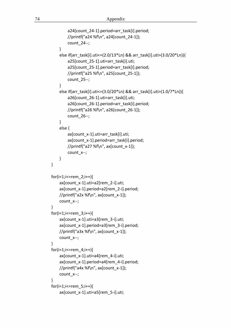
74 Appendix
a24[count_24-1].period=arr_task[i].period;
//printf("a24 %f\n", a24[count_24-1]);
count_24--;
}
else if(arr_task[i].uti<=(2.0/13*Ln) && arr_task[i].uti>(3.0/20*Ln)){
a25[count_25-1].uti=arr_task[i].uti;
a25[count_25-1].period=arr_task[i].period;
//printf("a25 %f\n", a25[count_25-1]);
count_25--;
}
else if(arr_task[i].uti<=(3.0/20*Ln) && arr_task[i].uti>(1.0/7*Ln)){
a26[count_26-1].uti=arr_task[i].uti;
a26[count_26-1].period=arr_task[i].period;
//printf("a26 %f\n", a26[count_26-1]);
count_26--;
}
else {
ax[count_x-1].uti=arr_task[i].uti;
ax[count_x-1].period=arr_task[i].period;
//printf("a27 %f\n", ax[count_x-1]);
count_x--;
}
}
for(i=1;i<=rem_2;i++){
ax[count_x-1].uti=a2[rem_2-i].uti;
ax[count_x-1].period=a2[rem_2-i].period;
//printf("a2x %f\n", ax[count_x-1]);
count_x--;
}
for(i=1;i<=rem_3;i++){
ax[count_x-1].uti=a3[rem_3-i].uti;
ax[count_x-1].period=a3[rem_3-i].period;
//printf("a3x %f\n", ax[count_x-1]);
count_x--;
}
for(i=1;i<=rem_4;i++){
ax[count_x-1].uti=a4[rem_4-i].uti;
ax[count_x-1].period=a4[rem_4-i].period;
//printf("a4x %f\n", ax[count_x-1]);
count_x--;
}
for(i=1;i<=rem_5;i++){
ax[count_x-1].uti=a5[rem_5-i].uti;

Appendix 75
ax[count_x-1].period=a5[rem_5-i].period;
//printf("a5x %f\n", ax[count_x-1]);
count_x--;
}
for(i=1;i<=rem_6;i++){
ax[count_x-1].uti=a6[rem_6-i].uti;
ax[count_x-1].period=a6[rem_6-i].period;
//printf("a6x %f\n", ax[count_x-1]);
count_x--;
}
for(i=1;i<=rem_7;i++){
ax[count_x-1].uti=a7[rem_7-i].uti;
ax[count_x-1].period=a7[rem_7-i].period;
//printf("a7x %f\n", ax[count_x-1]);
count_x--;
}
for(i=1;i<=rem_8;i++){
ax[count_x-1].uti=a8[rem_8-i].uti;
ax[count_x-1].period=a8[rem_8-i].period;
//printf("a8x %f\n", ax[count_x-1]);
count_x--;
}
for(i=1;i<=rem_9;i++){
ax[count_x-1].uti=a9[rem_9-i].uti;
ax[count_x-1].period=a9[rem_9-i].period;
//printf("a9x %f\n", ax[count_x-1]);
count_x--;
}
for(i=1;i<=rem_10;i++){
ax[count_x-1].uti=a10[rem_10-i].uti;
ax[count_x-1].period=a10[rem_10-i].period;
//printf("a10x %f\n", ax[count_x-1]);
count_x--;
}
for(i=1;i<=rem_11;i++){
ax[count_x-1].uti=a11[rem_11-i].uti;
ax[count_x-1].period=a11[rem_11-i].period;
//printf("a11x %f\n", ax[count_x-1]);
count_x--;
}
for(i=1;i<=rem_12;i++){
ax[count_x-1].uti=a12[rem_12-i].uti;
ax[count_x-1].period=a12[rem_12-i].period;
//printf("a12x %f\n", ax[count_x-1]);

76 Appendix
count_x--;
}
for(i=1;i<=rem_13;i++){
ax[count_x-1].uti=a13[rem_13-i].uti;
ax[count_x-1].period=a13[rem_13-i].period;
//printf("a13x %f\n", ax[count_x-1]);
count_x--;
}
for(i=1;i<=rem_14;i++){
ax[count_x-1].uti=a14[rem_14-i].uti;
ax[count_x-1].period=a14[rem_14-i].period;
//printf("a14x %f\n", ax[count_x-1]);
count_x--;
}
for(i=1;i<=rem_15;i++){
ax[count_x-1].uti=a15[rem_15-i].uti;
ax[count_x-1].period=a15[rem_15-i].period;
//printf("a15x %f\n", ax[count_x-1]);
count_x--;
}
for(i=1;i<=rem_16;i++){
ax[count_x-1].uti=a16[rem_16-i].uti;
ax[count_x-1].period=a16[rem_16-i].period;
//printf("a16x %f\n", ax[count_x-1]);
count_x--;
}
for(i=1;i<=rem_17;i++){
ax[count_x-1].uti=a17[rem_17-i].uti;
ax[count_x-1].period=a17[rem_17-i].period;
//printf("a17x %f\n", ax[count_x-1]);
count_x--;
}
for(i=1;i<=rem_18;i++){
ax[count_x-1].uti=a18[rem_18-i].uti;
ax[count_x-1].period=a18[rem_18-i].period;
//printf("a18x %f\n", ax[count_x-1]);
count_x--;
}
for(i=1;i<=rem_19;i++){
ax[count_x-1].uti=a19[rem_19-i].uti;
ax[count_x-1].period=a19[rem_19-i].period;
//printf("a19x %f\n", ax[count_x-1]);
count_x--;
}

Appendix 77
for(i=1;i<=rem_20;i++){
ax[count_x-1].uti=a20[rem_20-i].uti;
ax[count_x-1].period=a20[rem_20-i].period;
//printf("a20x %f\n", ax[count_x-1]);
count_x--;
}
for(i=1;i<=rem_21;i++){
ax[count_x-1].uti=a21[rem_21-i].uti;
ax[count_x-1].period=a21[rem_21-i].period;
//printf("a21x %f\n", ax[count_x-1]);
count_x--;
}
for(i=1;i<=rem_22;i++){
ax[count_x-1].uti=a22[rem_22-i].uti;
ax[count_x-1].period=a22[rem_22-i].period;
//printf("a22x %f\n", ax[count_x-1]);
count_x--;
}
for(i=1;i<=rem_23;i++){
ax[count_x-1].uti=a23[rem_23-i].uti;
ax[count_x-1].period=a23[rem_23-i].period;
//printf("a23x %f\n", ax[count_x-1]);
count_x--;
}
for(i=1;i<=rem_24;i++){
ax[count_x-1].uti=a24[rem_24-i].uti;
ax[count_x-1].period=a24[rem_24-i].period;
//printf("a24x %f\n", ax[count_x-1]);
count_x--;
}
for(i=1;i<=rem_25;i++){
ax[count_x-1].uti=a25[rem_25-i].uti;
ax[count_x-1].period=a25[rem_25-i].period;
//printf("a25x %f\n", ax[count_x-1]);
count_x--;
}
for(i=1;i<=rem_26;i++){
ax[count_x-1].uti=a26[rem_26-i].uti;
ax[count_x-1].period=a26[rem_26-i].period;
//printf("a26x %f\n", ax[count_x-1]);
count_x--;
}
free(a2);

78 Appendix
a2=NULL;
free(a3);
a3=NULL;
free(a4);
a4=NULL;
free(a5);
a5=NULL;
free(a6);
a6=NULL;
free(a7);
a7=NULL;
free(a8);
a8=NULL;
free(a9);
a9=NULL;
free(a10);
a10=NULL;
free(a11);
a11=NULL;
free(a12);
a12=NULL;
free(a13);
a13=NULL;
free(a14);
a14=NULL;
free(a15);
a15=NULL;
free(a16);
a16=NULL;
free(a17);
a17=NULL;
free(a18);
a18=NULL;
free(a19);
a19=NULL;
free(a20);
a20=NULL;
free(a21);
a21=NULL;
free(a22);
a22=NULL;
free(a23);
a23=NULL;
free(a24);

Appendix 79
a24=NULL;
free(a25);
a25=NULL;
free(a26);
a26=NULL;
x_uti=0;
for(i=0;i<x;i++) x_uti=x_uti+ax[i].uti;
//printf("x_uti %f\n",x_uti);
count_pre=0;
count_norm=0;
uti=(double*)malloc(x*sizeof(double));
pre=(task*)malloc(x*sizeof(task));
norm=(task*)malloc(x*sizeof(task));
for(i=0;i<x-1;i++){
for(j=i+1;j<x;j++){
if(ax[j].period<ax[i].period){
tmp=ax[i].period;
ax[i].period=ax[j].period;
ax[j].period=tmp;
tmp=ax[i].uti;
ax[i].uti=ax[j].uti;
ax[j].uti=tmp;
}
}
}
//for(i=0;i<x;i++) printf("ax %f\n",ax[i]);
tmp=0;
for(i=0;i<x;i++){
tmp=tmp+ax[i].uti;
uti[i]=x_uti-tmp;
//printf("uti[] %f\n", uti[i]);
//printf("proc_num %d\n", proc_num);
c=(proc_num-1)*new_theta;
//printf("c %f\n", c);
if(i!=x-1 && ax[i].uti>new_weight && uti[i]<=c){
pre[count_pre].uti=ax[i].uti;
//printf("ax[] %f pre[] %f\n", ax[i].uti, pre[count_pre].uti);
pre[count_pre].period=ax[i].period;
count_pre++;
80 Appendix
proc_num--;
}
else {
norm[count_norm].uti=ax[i].uti;
norm[count_norm].period=ax[i].period;
count_norm++;
}
}
free(uti);
uti=NULL;
free(ax);
ax=NULL;
for(i=0;i<count_pre-1;i++){
for(j=i+1;j<count_pre;j++){
if(pre[j].period>pre[i].period){
tmp=pre[i].period;
pre[i].period=pre[j].period;
pre[j].period=tmp;
tmp=pre[i].uti;
pre[i].uti=pre[j].uti;
pre[j].uti=tmp;
}
}
}
//for(i=0;i<count_pre;i++) printf("pre[] %f\n",pre[i].uti);
//for(i=0;i<count_norm;i++) printf("norm[] %f\n",norm[i].uti);
pre_cpu=(double*)malloc(count_pre*sizeof(double));
norm_cpu=(double*)malloc(proc_num*sizeof(double));
subtask=(int*)malloc(count_norm*sizeof(int));
for(i=0;i<count_pre;i++) pre_cpu[i]=pre[i].uti;
free(pre);
pre=NULL;
for(i=0;i<proc_num;i++) norm_cpu[i]=0;
for(i=0;i<count_norm;i++) subtask[i]=1;
n=proc_num;
m=count_pre;
p=count_norm;
i=0;

Appendix 81
t=0;
flg=0;
printf("CHAOX pre %d, norm %d, x %d, proc_num %d\n", m, p, x, n);
while(count_norm>0){
while(proc_num>0){
if((norm_cpu[0]+norm[i].uti)<=new_theta){
norm_cpu[0]=norm_cpu[0]+norm[i].uti;
//printf("norm[i].uti %f\n", norm[i].uti);
//printf("norm_cpu[0] %f\n",norm_cpu[0]);
count_norm--;
if(norm_cpu[0]==new_theta) {
proc_num--;
printf("Retard\n");
}
for(j=0;j<n-1;j++){
for(k=j+1;k<n;k++){
if(norm_cpu[k]<norm_cpu[j]){
tmp=norm_cpu[j];
norm_cpu[j]=norm_cpu[k];
norm_cpu[k]=tmp;
}
}
}
i++;
if(count_norm==0) break;
}
else {
//printf("~~1norm[i].uti %f\n", norm[i].uti);
norm[i].uti=norm[i].uti-(new_theta-norm_cpu[0]);
//printf("~~2norm[i].uti %f\n", norm[i].uti);
norm_cpu[0]=new_theta;
//printf("~~norm_cpu[0] %f\n",norm_cpu[0]);
proc_num--;
subtask[i]++;
for(j=0;j<n-1;j++){
for(k=j+1;k<n;k++){
if(norm_cpu[k]<norm_cpu[j]){
tmp=norm_cpu[j];
norm_cpu[j]=norm_cpu[k];
norm_cpu[k]=tmp;
}
}
}

82 Appendix
if(proc_num==0) break;
}
}
if(count_norm==0) break;
while(count_pre>0){
while(t<m){
if((pre_cpu[t]+norm[i].uti)<=new_theta){
//printf("i %d\n", i);
//printf("t %d\n", t);
pre_cpu[t]=pre_cpu[t]+norm[i].uti;
//printf("``norm[i].uti %f\n", norm[i].uti);
//printf("``pre_cpu[0] %f\n",pre_cpu[t]);
count_norm--;
i++;
if(pre_cpu[t]==new_theta){
t++;
count_pre--;
printf("Retard\n");
}
if(count_norm==0) break;
}
else {
//printf("^^1norm[i].uti %f\n", norm[i].uti);
norm[i].uti=norm[i].uti-(new_theta-pre_cpu[t]);
//printf("^^2norm[i].uti %f\n", norm[i].uti);
pre_cpu[t]=new_theta;
//printf("^^pre_cpu[0] %f\n",pre_cpu[t]);
t++;
//printf("t %d\n", t);
count_pre--;
subtask[i]++;
}
}
if(count_norm==0) break;
}
if(count_pre==0 && proc_num==0) {
printf("! CHAOX ASSIGNMENT FAILED 1\n");
flg=1;
chaox_return=1;
break;
}
}
free(norm);
norm=NULL;

Appendix 83
for(i=0;i<p-1;i++){
for(j=i+1;j<p;j++){
if(subtask[j]>subtask[i]){
tmp=subtask[i];
subtask[i]=subtask[j];
subtask[j]=tmp;
}
}
}
for(i=0;i<p;i++){
//printf("subtask[] %d\n", subtask[i]);
if(subtask[i]!=1) chaox_split++;
}
if(chaox_sub<subtask[0]) chaox_sub=subtask[0];
if(flg==1) {
chaox_split=0;
chaox_sort=0;
chaox_sub=0;
}
if(flg!=1){
double temp=0;
for(i=0;i<m;i++) temp=temp+pre_cpu[i];
for(i=0;i<n;i++) temp=temp+norm_cpu[i];
printf("CHAOX Uti CPU %f, Uti Tot %f\n",temp, x_uti);
}
free(pre_cpu);
pre_cpu=NULL;
free(norm_cpu);
norm_cpu=NULL;
free(subtask);
subtask=NULL;
}
else if(proc_num==0 && x>0){
printf("! CHAOX ASSIGNMENT FAILED 2\n");
chaox_return=1;
chaox_split=0;
chaox_sort=0;
chaox_sub=0;
}
else if(proc_num<0){
printf("! CHAOX ASSIGNMENT FAILED 3\n");

84 Appendix
chaox_return=1;
chaox_split=0;
chaox_sort=0;
chaox_sub=0;
}
}
double neu()
{
int i, j, k, t, m, n, p, flg, norm_num, count_pre, count_norm;
double tmp, tsk_uti, c;
task *tsk, *pre, *norm;
double *uti, *pre_cpu, *norm_cpu;
int *subtask;
neu_return=0;
neu_split=0;
neu_sort=task_num;
tsk=(task*)malloc(task_num*sizeof(task));
for(i=0;i<task_num;i++){
tsk[i].uti=arr_task[i].uti;
tsk[i].period=arr_task[i].period;
}
tsk_uti=0;
for(i=0;i<task_num;i++) tsk_uti=tsk_uti+tsk[i].uti;
count_pre=0;
count_norm=0;
norm_num=PROC;
pre=(task*)malloc(task_num*sizeof(task));
norm=(task*)malloc(task_num*sizeof(task));
uti=(double*)malloc(task_num*sizeof(double));
for(i=0;i<task_num-1;i++){
for(j=i+1;j<task_num;j++){
if(tsk[j].period<tsk[i].period){
tmp=tsk[i].period;
tsk[i].period=tsk[j].period;
tsk[j].period=tmp;
tmp=tsk[i].uti;
tsk[i].uti=tsk[j].uti;
tsk[j].uti=tmp;
}

Appendix 85
}
}
//for(i=0;i<task_num;i++) printf("tsk[] %f\n",tsk[i]);
tmp=0;
for(i=0;i<task_num;i++){
tmp=tmp+tsk[i].uti;
uti[i]=tsk_uti-tmp;
c=(norm_num-1)*theta;
if(i!=task_num-1 && tsk[i].uti>weight && uti[i]<=c){
pre[count_pre].uti=tsk[i].uti;
pre[count_pre].period=tsk[i].period;
//printf("pre %f\n",pre[count_pre]);
count_pre++;
norm_num--;
}
else {
norm[count_norm].uti=tsk[i].uti;
norm[count_norm].period=tsk[i].period;
//printf("norm %f\n",norm[count_norm]);
count_norm++;
}
}
for(i=0;i<count_pre-1;i++){
for(j=i+1;j<count_pre;j++){
if(pre[j].period>pre[i].period){
tmp=pre[i].period;
pre[i].period=pre[j].period;
pre[j].period=tmp;
tmp=pre[i].uti;
pre[i].uti=pre[j].uti;
pre[j].uti=tmp;
}
}
}
free(tsk);
tsk=NULL;
free(uti);
uti=NULL;
pre_cpu=(double*)malloc(count_pre*sizeof(double));
norm_cpu=(double*)malloc(norm_num*sizeof(double));

86 Appendix
for(i=0;i<count_pre;i++) pre_cpu[i]=pre[i].uti;
free(pre);
pre=NULL;
subtask=(int*)malloc(count_norm*sizeof(int));
for(i=0;i<norm_num;i++) norm_cpu[i]=0;
for(i=0;i<count_norm;i++) subtask[i]=1;
n=norm_num;
m=count_pre;
p=count_norm;
i=0;
t=0;
flg=0;
while(count_norm>0){
while(norm_num>0){
if((norm_cpu[0]+norm[i].uti)<=theta){
norm_cpu[0]=norm_cpu[0]+norm[i].uti;
//printf("norm[i].uti %f\n", norm[i].uti);
//printf("norm_cpu[0] %f\n",norm_cpu[0]);
count_norm--;
if(norm_cpu[0]==theta) norm_num--;
for(j=0;j<n-1;j++){
for(k=j+1;k<n;k++){
if(norm_cpu[k]<norm_cpu[j]){
tmp=norm_cpu[j];
norm_cpu[j]=norm_cpu[k];
norm_cpu[k]=tmp;
}
}
}
i++;
if(count_norm==0) break;
}
else {
//printf("~~1norm[i].uti %f\n", norm[i].uti);
norm[i].uti=norm[i].uti-(theta-norm_cpu[0]);
//printf("~~2norm[i].uti %f\n", norm[i].uti);
norm_cpu[0]=theta;
//printf("~~norm_cpu[0] %f\n",norm_cpu[0]);
norm_num--;
subtask[i]++;
for(j=0;j<n-1;j++){
for(k=j+1;k<n;k++){

Appendix 87
if(norm_cpu[k]<norm_cpu[j]){
tmp=norm_cpu[j];
norm_cpu[j]=norm_cpu[k];
norm_cpu[k]=tmp;
}
}
}
if(norm_num==0) break;
}
}
if(count_norm==0) break;
while(count_pre>0){
while(t<m){
if((pre_cpu[t]+norm[i].uti)<=theta){
//printf("i %d\n", i);
//printf("t %d\n", t);
pre_cpu[t]=pre_cpu[t]+norm[i].uti;
//printf("``norm[i].uti %f\n", norm[i].uti);
//printf("``pre_cpu[0] %f\n",pre_cpu[t]);
count_norm--;
i++;
if(pre_cpu[t]==theta){
t++;
count_pre--;
}
if(count_norm==0) break;
}
else {
//printf("^^1norm[i].uti %f\n", norm[i].uti);
norm[i].uti=norm[i].uti-(theta-pre_cpu[t]);
//printf("^^2norm[i].uti %f\n", norm[i].uti);
pre_cpu[t]=theta;
//printf("^^pre_cpu[0] %f\n",pre_cpu[t]);
t++;
//printf("t %d\n", t);
count_pre--;
subtask[i]++;
}
}
if(count_norm==0) break;
}
if(count_pre==0 && norm_num==0) {
printf("! NEU ASSIGNMENT FAILED\n");
flg=1;

88 Appendix
neu_return=1;
break;
}
}
free(norm);
pre=NULL;
if(flg==0){
for(i=0;i<p-1;i++){
for(j=i+1;j<p;j++){
if(subtask[j]>subtask[i]){
tmp=subtask[i];
subtask[i]=subtask[j];
subtask[j]=tmp;
}
}
}
for(i=0;i<p;i++){
//printf("subtask[] %d\n", subtask[i]);
if(subtask[i]!=1) neu_split++;
}
if(neu_sub<subtask[0]) neu_sub=subtask[0];
double temp=0;
for(i=0;i<m;i++) temp=temp+pre_cpu[i];
for(i=0;i<n;i++) temp=temp+norm_cpu[i];
printf("NEU Uti CPU %f, Uti Tot %f\n",temp, tsk_uti);
printf("NEU pre %d, norm %d\n", m, n);
}
else {
neu_split=0;
neu_sort=0;
neu_sub=0;
}
free(pre_cpu);
pre_cpu=NULL;
free(norm_cpu);
norm_cpu=NULL;
free(subtask);
subtask=NULL;
}

Appendix 89
main()
{
int i, j;
int chaox_tot_split=0;
int chaox_max_subtask=0;
int chaox_tot_sort=0;
double chaox_tot_task=0;
double chaox_ok=0;
int neu_tot_split=0;
int neu_max_subtask=0;
int neu_tot_sort=0;
double neu_ok=0;
double sys_uti, ratio;
int n=0;
int m=0;
typedef struct{
int succ;
int fail;
} bucket;
bucket chaox_bucket[100], neu_bucket[100];
double chaox_graph[100], neu_graph[100];
for(i=0;i<100;i++){
chaox_bucket[i].succ=0;
chaox_bucket[i].fail=0;
neu_bucket[i].succ=0;
neu_bucket[i].fail=0;
}
srand((unsigned)time(0));
for(i=0;i<SET;i++){
init();
sys_uti=(tot_uti/PROC)*100;
for(j=0;j<100;j++){
if(sys_uti<j+1) break;
}
//printf("j %d\n",j);
chaox();
chaox_tot_split=chaox_tot_split+chaox_split;
if(chaox_max_subtask<chaox_sub) chaox_max_subtask=chaox_sub;
chaox_tot_sort=chaox_tot_sort+chaox_sort;
neu();
neu_tot_split=neu_tot_split+neu_split;
neu_tot_sort=neu_tot_sort+neu_sort;
if(neu_max_subtask<neu_sub) neu_max_subtask=neu_sub;
90 Appendix
if(chaox_return==0) {
chaox_ok++;
chaox_bucket[j].succ++;
}
if(neu_return==0) {
neu_ok++;
neu_bucket[j].succ++;
}
if(chaox_return) chaox_bucket[j].fail++;
if(neu_return) neu_bucket[j].fail++;
printf("chx succ %d, chx fail %d\n", chaox_bucket[j].succ,
chaox_bucket[j].fail);
printf("neu succ %d, neu fail %d\n", neu_bucket[j].succ, neu_bucket[j].fail);
if(chaox_return==0 && neu_return) n++;
if(chaox_return && neu_return==0) m++;
//if(m>0) sleep(100000);
/*if(chaox_return && neu_return){
task_num=PROC+N;
i--;
printf("TASK RESET~~~~~~~~~~\n");
//sleep(1);
}
else*/
task_num++;
printf("CHAOX_OK %f NEU_OK %f\n", chaox_ok, neu_ok);
printf("No.SET %d TASK NUM %d\n", i+1, task_num);
printf("---------------------------------------------\n");
printf("---------------------------------------------\n");
//if(chaox_bucket[68].fail>0) sleep(100000);
}
for(i=0;i<100;i++){
chaox_graph[i]=((double)chaox_bucket[i].succ)/(chaox_bucket[i].succ+chaox_bu
cket[i].fail);
neu_graph[i]=((double)neu_bucket[i].succ)/(neu_bucket[i].succ+neu_bucket[i].f
ail);
printf("%d %f\n",i, chaox_graph[i]);
}
printf("+++++++++++++++++++++++++++++++++++++++++++++\n");
for(i=0;i<100;i++) printf("%d %f\n",i, neu_graph[i]);
printf("CHAOX\nOK %f\nTot Split %d\nAvg Split %f\nMax. Subtask %d\nTotal
Sorted %d\nAvg Sorted %f\nAverage Ratio %f\n", chaox_ok, chaox_tot_split,

Appendix 91
chaox_tot_split/chaox_ok, chaox_max_subtask, chaox_tot_sort,
chaox_tot_sort/chaox_ok, chaox_ok/SET);
printf("+++++++++++++++++++++++++++++++++++++++++++++\n");
printf("NEU\nOK %f\nTot Split %d\nAvg Split %f\nMax. Subtask %d\nTotal
Sorted %d\nAvg Sorted %f\nAverage Ratio %f\n", neu_ok, neu_tot_split,
neu_tot_split/neu_ok, neu_max_subtask, neu_tot_sort, neu_tot_sort/neu_ok,
neu_ok/SET);
printf("+++++++++++++++++++++++++++++++++++++++++++++\n");
printf("Dominant Value n %d m %d\n", n, m);
printf("+++++++++++++++++++++++++++++++++++++++++++++\n");
}