Embed Size (px)
Citation preview
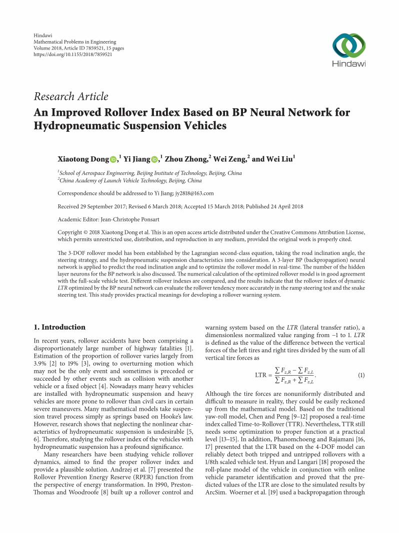
Research ArticleAn Improved Rollover Index Based on BP Neural Network forHydropneumatic Suspension Vehicles
Xiaotong Dong 1 Yi Jiang 1 Zhou Zhong2 Wei Zeng2 andWei Liu1
1School of Aerospace Engineering Beijing Institute of Technology Beijing China2China Academy of Launch Vehicle Technology Beijing China
Correspondence should be addressed to Yi Jiang jy2818163com
Received 29 September 2017 Revised 6 March 2018 Accepted 15 March 2018 Published 24 April 2018
Academic Editor Jean-Christophe Ponsart
Copyright copy 2018 Xiaotong Dong et alThis is an open access article distributed under the Creative Commons Attribution Licensewhich permits unrestricted use distribution and reproduction in any medium provided the original work is properly cited
The 3-DOF rollover model has been established by the Lagrangian second-class equation taking the road inclination angle thesteering strategy and the hydropneumatic suspension characteristics into consideration A 3-layer BP (backpropagation) neuralnetwork is applied to predict the road inclination angle and to optimize the rollover model in real-timeThe number of the hiddenlayer neurons for the BP network is also discussedThe numerical calculation of the optimized rollover model is in good agreementwith the full-scale vehicle test Different rollover indexes are compared and the results indicate that the rollover index of dynamicLTR optimized by the BP neural network can evaluate the rollover tendencymore accurately in the ramp steering test and the snakesteering test This study provides practical meanings for developing a rollover warning system
1 Introduction
In recent years rollover accidents have been comprising adisproportionately large number of highway fatalities [1]Estimation of the proportion of rollover varies largely from39 [2] to 19 [3] owing to overturning motion whichmay not be the only event and sometimes is preceded orsucceeded by other events such as collision with anothervehicle or a fixed object [4] Nowadays many heavy vehiclesare installed with hydropneumatic suspension and heavyvehicles are more prone to rollover than civil cars in certainsevere maneuvers Many mathematical models take suspen-sion travel process simply as springs based on Hookersquos lawHowever research shows that neglecting the nonlinear char-acteristics of hydropneumatic suspension is undesirable [56] Therefore studying the rollover index of the vehicles withhydropneumatic suspension has a profound significance
Many researchers have been studying vehicle rolloverdynamics aimed to find the proper rollover index andprovide a plausible solution Andrzej et al [7] presented theRollover Prevention Energy Reserve (RPER) function fromthe perspective of energy transformation In 1990 Preston-Thomas and Woodroofe [8] built up a rollover control and
warning system based on the LTR (lateral transfer ratio) adimensionless normalized value ranging from minus1 to 1 LTRis defined as the value of the difference between the verticalforces of the left tires and right tires divided by the sum of allvertical tire forces as
LTR = sum119865119911119877 minus sum119865119911119871sum119865119911119877 + sum119865119911119871 (1)
Although the tire forces are nonuniformly distributed anddifficult to measure in reality they could be easily reckonedup from the mathematical model Based on the traditionalyaw-roll model Chen and Peng [9ndash12] proposed a real-timeindex called Time-to-Rollover (TTR) Nevertheless TTR stillneeds some optimization to proper function at a practicallevel [13ndash15] In addition Phanomchoeng and Rajamani [1617] presented that the LTR based on the 4-DOF model canreliably detect both tripped and untripped rollovers with a18th scaled vehicle test Hyun and Langari [18] proposed theroll-plane model of the vehicle in conjunction with onlinevehicle parameter identification and proved that the pre-dicted values of the LTR are close to the simulated results byArcSim Woerner et al [19] used a backpropagation through
HindawiMathematical Problems in EngineeringVolume 2018 Article ID 7859521 15 pageshttpsdoiorg10115520187859521
2 Mathematical Problems in Engineering
yz
x
R
Drivingvelocity
(x0 y0)
(x1 y1)
i
Fxi
Fxi
Fyi
Fyi
ay0ay1
ℎ sin
Figure 1 Top view of rollover model in global coordinates
time algorithm to model and predict the rollover of a tanktruck carrying varying liquid volumes However the roadinclination angle has great influence on the rollover statuswhich has not been clearly addressed in the study of rolloverAs the road inclination angle is difficult to obtain directlyit is necessary to establish the relationship between the roadinclination angle and other vehicle dynamic parameters
As widely employed in the field of machine learning andcognitive science the artificial neural network is amathemat-ical computationalmodel network inspired by biological neu-ral networks used to demonstrate the complicated nonlinearrelationship [20] The backpropagation (BP) neural networkis a type of the most commonly used neural network withan error backpropagation algorithm that is one of the mostpopularized and efficient methods for network optimization[21] By means of the BP neural network the effect of theroad inclination angle could be reflexed in the vehicle rolloverdynamics
The structure of the paper is organized as follows inSection 2 based on the Lagrangian second-class equationa vehicle rollover model on the sloping road is establishedThe nonlinear hydropneumatic suspension characteristicsare discussed to deduce the vehicle equivalent stiffness anddamping coefficient An example of the model numerical
calculation is analyzed in detail In Section 3 a BP neuralnetwork using a hyperbolic tangent function as the transferfunction is applied to optimize the rollover model Rolloverindexes are presented based on the conception of LTRSection 4 begins with a brief introduction on the full-sizevehicle test Then the results of the numerical calculation arediscussed and several rollover indexes are put into compari-son Finally in Section 5 some conclusions are summarizedfor further studying
2 Modeling
In this section a 3-DOF rollover model considering the roadinclination angle has been established The basic assumptionis that sprung mass has only roll motion relative to theunsprung mass and the unsprung mass has no pitch motionor roll motion Notice that to clear the confusion of positivesign and negative sign all signs of the undeclared values arefollowing the specified coordinate system below
21 Rollover Model Based on Lagrangian Second-Class Equa-tion The global coordinates are defined as 119911-axis verticaldown to the ground and the yaw angle of the vehicle 120574 asshown in Figure 1
Mathematical Problems in Engineering 3
x y
z
O
(b)(a)
h
m1
C1
C0
ay1
m1gℎ1
ℎ0
m0
m0
m1
ay0
m0gFyL
FzLFzR
FyR
r 0
Mx
= r + 0
Figure 2 (a) Rear view of rollover model in the specified local coordinates (b) Internal force and position relationship between sprung massand unsprung mass
The positions of the sprung mass 1198981 and the unsprungmass1198980 are given as (1199091 1199101) and (1199090 1199100) With the influenceof external factors sprung mass 1198981 will slightly roll a smallangle 120579 and change the relative position between 1198981 and 1198980Given that the roll radius is ℎ then the displacement between1198981 and1198980 in 119909119910 plane is ℎ sin 120579 then there is
1199091 = 1199090 minus ℎ sin 120579 sin 1205741199101 = 1199100 + ℎ sin 120579 cos 120574 (2)
As 120579 is rather small there are sin 120579 asymp 120579 and cos 120579 asymp 1And respectively the lateral acceleration of1198980 and1198981 is
1198861199100 = minus0 sin 120574 + 1199100 cos 1205741198861199101 = minus1 sin 120574 + 1199101 cos 120574 = 1198861199100 + ℎ ( 120579 minus 120579 1205742) (3)
The specified local coordinates fixed on the vehicle aredefined as119909-axis pointing to the vehicle front119910-axis pointingright and 119911-axis following the right-hand law as shown inFigure 2 Figure 2(a) demonstrates the overall force situationfor the whole mass while Figure 2(b) shows the internal forceand position relationship between sprungmass and unsprungmass
When the road inclination (or other factors that mayinduce the unsprung mass to roll) exists as 120579119903 it could bereckoned as the ground counterbalancing most of the gravityand the vehicle bearing an extra acceleration 119892 sin 120579119903 in the 119910direction It can be seen that the original roll angle 120579 consistsof the road inclination angle 120579119903 and the relative roll angle1205790 Road inclination angle 120579119903 is unknown and by ignoring itschanging rate then there is
120579 = 120579119903 + 1205790120579 = 1205790 (4)
and the total kinetic energy of the system is119879 = 1198790 + 1198791
= 121198980 (20 + 11991020) + 121198981 (21 + 11991021) + 12119869119911 1205742+ 12 (1198691119909 + 1198981ℎ2) 1205792
(5)
where 119869119911 is the 119911 moment of inertia of the whole mass 1198690119911is the 119911 moment of inertia of the unsprung mass 1198691119911 is the 119911moment of inertia of the sprungmass 1198690119909 is the 119909moment ofinertia of the unsprung mass 1198691119909 is the 119909 moment of inertiaof the sprung mass 120574 is yaw angular velocity 120596119911 and 120574 is yawangular acceleration 119911
According to the Lagrangian second-class equationchoosing 1199090 1199100 120579 120574 as the generalized coordinates then inthe global coordinates there is
119898 cos 0 minus 1198981ℎ( 120579 sin 120574 + 120579 cos 120574 + 119889 (120579 120574)119889119905 cos 120574
minus 120579 120574 sin 120574) = sum119865119909 cos 120574 minus sum119865119910 sin 120574 minus 119898119892 sin 120579119903sdot sin 120574
119898 cos 1199100 minus 1198981ℎ(minus 120579 cos 120574 + 120579 sin 120574 + 119889 (120579 120574)119889119905 sin 120574
+ 120579 120574 cos 120574) = sum119865119909 sin 120574 + sum119865119910 cos 120574 + 119898119892 sin 120579119903sdot cos 120574
(1198691119909 + 21198981ℎ2) 120579 + 1198981ℎ (minus0 sin 120574 + 119910 cos 120574)minus 1198981ℎ2 1205742120579 = 1198981119892ℎ sin 120579 + 119872119909
(1198690119911 + 1198691119911) 120574 = sum119865119910119894 sdot 119897119894
(6)
4 Mathematical Problems in Engineering
Inside
Outside
N
Axle N Axle Nminus 1 Axle i
x
y Axle 1Axle 2Axle 3
Fy3 Fy2 Fy1
1
l12
Turningdirection
dGMM
dNOLH
l2l3
lNminus1
OC
lNNminus1
FyN FyNminus1
Figure 3 Ackerman steering for multiaxle vehicles
where119872119909 is the antiroll moment applied on sprungmass andits calculation will be discussed later in Section 22 119865119909 119865119910 arethe component forces of one tire in local coordinates 119897119894 is thedistance between axle 119894 and themass center with positive signif axle 119894 is ahead of the mass center or negative sign if it isbehind the mass center
In rollover model researchers are more interested in thevehicle lateral dynamics Take (3) and (4) into (6) and rewriteit as
1198981198861199100 + 1198981ℎ [ 1205790 minus (120579119903 + 1205790) 1205962119911] = sum119865119910 + 119898119892 sin 120579119903(1198691119909 + 21198981ℎ2) 1205790 + 1198981ℎ1198861199100 minus 1198981ℎ21205962119911 (120579119903 + 1205790)
= 1198981119892ℎ sin (120579119903 + 1205790) + 119872119909(1198690119911 + 1198691119911) 119911 = sum119865119910119894 sdot 119897119894
(7)
Equation (7) is the rollover model in the local coordinatesThe vehiclersquos lateral dynamics include circling motion andlateral skid motion and then there is
1198861199100 = 119910 + 120596119911119881119909 (8)
where 119881119910 is the lateral velocity of vehicle mass center and 119881119909is the forward velocity of vehicle mass center Therefore theslip angle of tire 119894 is
120572119894 = arctan119881119910 + 120596119911119897119894119881119909 minus 120596119911119861119894 minus 120575119894 (9)
where 119861119894 is half of the track width for left tires 119861119894 = 119861 andfor right tires 119861119894 = minus119861 120575119894 is the steering angle of tire 119894 andit is decided by the steering strategy which will be discussedsoon
As for 119865119910119894 there is119865119910119894 = 119865119910119894 sdot cos 120575119894 = 119896119905120572119894 sdot cos 120575119894
= 119896119905 sdot cos 120575119894 (arctan 119881119910 + 120596119911119897119894119881119909 minus 120596119911119861119894 minus 120575119894) 119896119905 lt 0 (10)
where 119865119910119894 is the lateral force of tire 119894 in tire local coordinatesand 119896119905 is the tire lateral stiffness
In order to keep the consistency in the numerical calcu-lation and the test according to the adopted steering anglemeasuring instrument for the test positive steering wheelangle 120575st indicates turning leftTherefore when in left turningscenario the signs of the steering wheel angle 120575st and the rollangle 120579 are positive and the signs of lateral acceleration 119886119910and yaw angular velocity 120596119911 are negative According to thatall variables are signed which makes the model calculationstandardized These agreements could clear the confusioncaused by different sign declarations
22 Ackerman Steering Strategy For multiaxle vehicleswhich have quite a long chassis and several steering axlesAckerman steering strategy is commonly applied [22] Ack-erman steering is very suitable for heavy-duty vehicles Oneof its principal benefits is to mitigate tire wear chassis stressand tire-road additional drag force The Ackerman steeringstrategy for multiaxle vehicles can be illustrated in Figure 3119873 is defined as the number of axles and 2119873 is the number oftires Notice that point 1198741015840 is the turning center of the vehicleand point 119862 is the vehicle mass center The turning center 1198741015840is used to calculate the yaw angular velocity 120596119911 These twopoints are equivalent when the slip angle ofmass center keepsat zero
Applying Ackerman steering strategy there is
1198971015840119894tan 120575119894 =
1198971015840119895tan 120575119895
cot 120575119894out minus cot 120575119894in = 21198611198971015840119894 (11)
where 1198971015840119894 is the difference of 119909 coordinate between axle 119894 andthe turning center1198741015840 120575119894 is the steering angle of tire 119894 and 120575119894inand 120575119894out are the steering angle of the inner tire and the outertire for axle 119894 respectively
Multiaxle vehicles usually have several steering axles inthe front and some in the rear probablyThe unsteering axlesdo not participate in steering whichmeans that their steeringangle is zero A new variable 119902119894 is given to indicate which axlesare the steering ones and which ones are not 119902119894 equals onewhen axle 119894 is a steering axle and equals zero when axle 119894 is
Mathematical Problems in Engineering 5
(a)
Liquid
Gas
Damping hole
Air accumulator
Check valve
Annulus areaEffective area
(b)
Figure 4 (a) Photo of hydropneumatic spring for vehicle suspension (b) Structure of one typical kind of hydropneumatic spring
notWhen the linear ratio between the steering angle and 1205751inis given as 1198621205751 then there is
1205751in = 1198621205751120575st1205751out = arccot(cot 1205751in + 211986111989710158401 ) 120575119894in = arctan( 119897101584011989411989710158401 tan 1205751in) sdot 119902119894
120575119894out = arctan( 119897101584011989411989710158401 tan 1205751out) sdot 119902119894
(12)
where 119902123 = 1 and 119902456 = 0 When the steering angle 120575119894of each tire is obtained the lateral force of each tire could becalculated according to (10) The main parameters of the testvehicle are given in Table 1
23 Hydropneumatic Suspension Hydropneumatic suspen-sions are different from the conventional suspension Thehighlight features are compactness easy installation andmost importantly extra heavy payload Difficultmanufactureand high maintenance demands are its major drawbacksFigure 4(a) demonstrates a common type of hydropneumaticspring for heavy-duty vehicle suspensions They utilize inertgas as the elastic medium and oil liquid as a support anddampingmediumwhich combines elastic energy storage anddamping energy storage into one function unit as seen inFigure 4(b)
It is assumed that the suspension forces on the sprungmass act parallel to the sprung mass 119911-axis The elastic forceof the hydropneumatic suspension is mainly generated by the
Table 1 Main parameters of the test vehicle (WS-2900)
Parameter Value Unit119873 6 -1198981 55000 kg1198980 15000 kg119869119909 606119890 + 04 kgsdotm2119869119911 766119890 + 05 kgsdotm2ℎ 12 m119861 14 m119867 192 m119892 98 kgsdotms2
k (constant) 30119890 + 06 Nrad119888 (constant) 20119890 + 04 Nsdotsrad119896119905 4720 Ndeg
piston pushing the liquid to compress the gas in the air accu-mulator therefore it shows obvious nonlinear characteristicsAccording to ideal gas state equation the change of the gasstate during the vehicle suspension vibration can be regardedas an adiabatic process where the gas polytropic exponent119903 = 14 Then the dynamic pressure is [23ndash25]
119875119904 = 119875119901119881119903119901(119881119901 + 119860119901Δ119911)119903 = 119875119901 (1 + Δ119911119911119901 )
minus119903 (13)
where 119875119901 is the balanced pressure 119881119901 is the balanced airvolume 119860119901 is the effective area of supporting effect 119911119901 isthe balanced deformation of the hydropneumatic spring Δ119911is the deformation of the hydropneumatic spring extensionscenario provides Δ119911 gt 0 and compression scenario providesΔ119911 lt 0
6 Mathematical Problems in Engineering
minus10
minus8
minus6
minus4
minus2Fk(N
)
minus150 minus100 minus50 0 50 100 150
Δz (mm)
times104
(a)
minus015 minus01 minus005 0 005 01 0150
2
4
6
8
10
Δz (mm)
times105
k(Δ
z)
(Nm
)
(b)
Figure 5 (a) Elastic force versus deformation of one hydropneumatic spring (b) Stiffness versus deformation of one hydropneumatic spring
Therefore according to the specified coordinates thesupport force applied on the spring on is written as
119865119896 = minus119875119904119860119901 = minus119875119901119860119901 (1 + Δ119911119911119901 )minus119903 (14)
It can be seen that the stiffness of hydropneumatic springbecomes larger if it is being compressed and vice versa asshown in Figure 5 This agrees with the compressibility lawof ideal gas
When the hydropneumatic spring is in the extensionscenario the damping force is generated only by the throttlingeffect of the damping hole when in the compression scenariothe damping force is generated by the damping hole andcheck valve together Therefore the damping force of onehydropneumatic spring could be written as [26]
119865119888 = sgn (Δ) 1205881198603119886Δ22 (119862119889119860119889 + 12119862119888119860119888
minus 12 sgn (Δ) 119862119888119860119888)minus2 (15)
where Δ is the velocity of the hydropneumatic spring defor-mation 120588 is the density of the oil liquid 119860119886 119862119888 119860119888 119862119889 and119860119889 are the dimensional parameters of the hydropneumaticspring And the sign function is defined as
sgn (Δ) = 1 extension (Δ gt 0)sgn (Δ) = minus1 compression (Δ lt 0) (16)
Figure 6 demonstrates the nonlinear damping characteristicsof one hydropneumatic spring As it can be seen the dampingforce increases rapidly in compression scenario but veryslowly in extension scenario It also shows that the dampingcoefficient is linearly related to the deformation velocity butit is obviously larger in the compression scenarioThis meansthat the damping influence of hydropneumatic spring mainlyfunctions in the extension scenario
When the roll movement of sprung mass agrees with theassumption in Figure 2(b) the deformations of one couple ofhydropneumatic springs installed left and right on the vehicleare equal Therefore the roll angle 1205790 can be derived as
1205790 = Δ119911119879 (17)
where 119879 is the distance between the supporting points ofhydropneumatic springs and the vehicle symmetry plane
After the relationship between the roll angle and thedeformation of hydropneumatic springs is built the 119909moment applied on sprung mass includes two parts one partcaused by suspension stiffness is
1198721205790 = 119873 sdot 119879 (119865119896119877 minus 119865119896119871)= 119873 sdot 119875119901119860119901119879[(1 + 1198791205790119911119901 )minus119903 minus (1 minus 1198791205790119911119901 )minus119903] (18)
the other part caused by damping is
119872 1205790 = 119873 sdot 119879 (119865119888119877 minus 119865119888119871)= minussgn ( 1205790)119873
sdot 1198791205881198603119886 (119879 1205790)22 ((119862119889119860119889 + 119862119888119860119888)minus2 + (119862119889119860119889)minus2) (19)
In summary the roll moment yielded by the suspension is
119872119909 = 1198721205790 + 119872 1205790 (20)
In the linear model there is
119872119909 = minus1198961205790 minus 119888 1205790 119896 119888 is constant (21)
Mathematical Problems in Engineering 7
minus150 minus100 minus50 500 100 150minus500
0
500
1000
1500
Fc(N
)
Δz (mms)
(a)
0
05
1
15
2
25
minus015 minus01 minus005 0 005 01 015Δz (ms)
times104
c(Δz)
(N(
ms
))
(b)
Figure 6 (a) Damping force versus deformation velocity of one hydropneumatic spring (b) Damping coefficient versus deformation velocityof one hydropneumatic spring
If comparing (20) with (21) we can also find out that 119896 and 119888are no longer constant and they are given as
119896 (1205790) = minus11987212057901198891205790 = 119873 sdot 1198751199011198601199011198792119911119901sdot 119903 [(1 + 1198791205790119911119901 )minus119903minus1 + (1 minus 1198791205790119911119901 )minus119903minus1]
119888 ( 1205790) = minus119872 1205790119889 1205790 = 1205790 sdot sign ( 1205790)sdot [11987312058811986031198861198793 ((119862119889119860119889 + 119862119888119860119888)minus2 + (119862119889119860119889)minus2)]
(22)
It can be seen in Figure 7 that the equivalent stiffness of thesuspension increases rapidly as the roll angle increases andthe equivalent damping of the suspension is linearly relatedto the roll angle changing rate
Figure 8 shows how the nonlinear stiffness and dampingaffect the dynamic response of the roll angle The stiffness 119896greatly affects the roll angle static value And the damping 119888affects the response time of the roll angle and also causes somesteady-state fluctuations This suggests that the influence ofsuspension characteristics on the dynamic response of the rollangle is critical The main parameters of the hydropneumaticsuspension are listed in Table 2
24 Model Numerical Calculation An Example Assumingthat driving speed is constant 6ms the steering wheel inputangle and the given road inclination are shown in Figure 9(a)The steering wheel angle is 0∘ before 119905 = 10 s then it rises to600∘ between 10 and 13 seconds then it remains constantAnd at 119905 = 25 s it begins to drops to 100∘ and remainsunchanged for the rest time As to the road inclination itbegins to grow at 119905 = 5 s and then stays at about 29∘ until
Table 2 Hydropneumatic suspension parameters
Parameter Value UnitN 6 -T 096 m120588 865 kgm2119911119901 0253 m119860119901 79119890 minus 03 m2
119860 119888 7854119890 minus 05 m2119860119889 1964119890 minus 05 m2119862119888 068 -119862119889 068 -119860119886 35119890 minus 03 m2
119905 = 20 s that it drops to minus14∘ and with some slight fluctuatesall the way
For the sake of comparing and analyzing the workingtime is divided into five time periods as shown below
(A) 119905 = 0sim5 s no steering angle no road inclination angle(B) 119905 = 5sim10 s no steering angle road inclination angle
increases(C) 119905 = 10sim20 s steering angle increasing then unchang-
ing road inclination angle staying top value (around29∘)
(D) 119905 = 20sim25 s steering angle unchanging then decreas-ing road inclination dropping to bottom value(around minus14∘)
(E) 119905 = 25sim40 s steering angle staying at 100∘ roadinclination angle oscillating very slightly
These five time periods could represent a typical ramp steer-ing case with the influence of road inclination To validate the
8 Mathematical Problems in Engineering
minus6 minus4 minus2 0 2 4 625
3
35
4
45
5
55
0 (deg)
k(
0)
(Nr
ad)
times106
(a)
minus6 minus4 minus2 0 2 4 60
2
4
6
8
10
12
c( 0)
(N(
rad
s))
0 (degs)
times104
(b)
Figure 7 (a) Equivalent stiffness of suspension (b) Equivalent damping of suspension
Time (s)
0
05
1
15
2
25
3
35
k c variablec constantk constant
k c constantTest
(d
eg)
0 2 4 6 8 10 12
Figure 8 Dynamic response of roll angle with different 119896 and 119888 ofsuspension
model the results need to be thoroughly discussed Analysisof the roll angle results shown in Figure 9(b) is given below
(A) As there is no steering angle and no road inclinationangle 1205790 and 120579 are both zero
(B) As road inclination angle increases with no steeringangle 1205790 goes along with 120579119903
(C) As road inclination angle stays unchanged and thesteering angle begins to increase 1205790 follows the flatroad ramp steering case whichmeans that 1205790 changeswith the steering angle If steering angle is positive 1205790gets bigger if it is negative 1205790 gets smaller In this case1205790 is about 35∘ at 119905 = 18 s
(D) At 119905 = 20 s 120579119903 drops to the bottom quickly whichmeans that 1205790 should drop tooHowever the droppingmagnitude of 1205790 should less than that of 120579119903 because thepositive steering angle is trying to keep 1205790 positive At119905 = 23 s 1205790 is about 26∘ and 120579 is 113∘ Apparently thesteering angle is dominating in this time period
(E) Finally the steering angle decreases to a small positivevalue with a negative road inclination value At 119905 =36 s 1205790 is around 008∘ and 120579 is aroundminus139∘ the roadinclination is dominating the roll angle now
In conclusion the roll angle is influenced by the couplingeffect between the steering angle and the road inclinationangle whichmeans that its value is dominated by the steeringangle when the steering angle is big enough otherwise itis dominated by the road inclination angle instead Whatis more this relationship is difficult to predict Thereforea neural network is applied to establish the relationshipbetween them
3 Neural Network Model
31 BP Neural Network Modeling The BP neural networkhas the characteristics of propagating the errors backwardthrough the network after the signal forward propagationby computing the gradient for each synaptic link and nodalbias using the chain rule which has the powerful capacityfor nonlinear mapping to reveal the internal law of theexperimental data A typical BP neural network structure isgiven in Figure 10
The forward propagation of the hidden layer and theoutput layer can be expressed as
119900119896119895 = 119891119895(sum119894
119908119894119895119900119896119894) (23)
Mathematical Problems in Engineering 9
0 5 10 15 20 25 30 35 40Time (s)
minus100
0
100
200
300
400
500
600
700
minus2
minus1
0
1
2
3
4
5St
eerin
g w
heel
angl
eMN
(deg
)
Road
incli
natio
n in
put
r(d
eg)
(a)
0 5 10 15 20 25 30 35 40Time (s)
minus2
0
2
4
6
8
Roll
angl
es (d
eg)
0r
(b)
Figure 9 (a) Input parameters of the model (b) Calculation result of roll angles
Input layer Hidden layer(s) Output layer
wijwmi
wjp
Figure 10 Typical BP neural network structure
where 119891119895 is the 119895th transfer function 119908119894119895 is the connectionweight which represents the weight for the neurons 119894 in theprevious layer relative to the neurons 119895 in the current layer 119900119896119895and 119900119896119894 are the outputs of the neurons 119894 in the previous layerand the neurons 119895 in the current layer for training sample 119896respectively
In this case the transfer function is the hyperbolic tangentfunction given in
119891 (119906) = tanh (119906) (24)
and with
1198911015840 (119906) = 1 minus 1198912 (119906) (25)
The training error gradient for the output layer is expressedas
120575119896119895 = (1 minus 1199002119896119895) (119889119896119895 minus 119900119896119895) (26)
where120575119896119895 and119889119896119895 are the training error gradient and the targetvalue for the neurons 119895 in the output layer for training sample119896 respectively
The training error gradient for the hidden layer isexpressed as
120575119896119895 = (1 minus 1199002119896119895)sum119898
120575119896119898119908119898119895 (27)
In the current iteration step n the weights are updatedaccording to
Δ119908119895119894 (119899) = 120578BP120575119896119895 (119899) 119900119896119895 (119899) + 120572BPΔ119908119895119894 (119899 minus 1) (28)
where 120578BP is the learning rate of BP network 120572BP is a momen-tum term which could adjust the amount of corrections andavoid the local minimum [27]
Therefore the new weights are updated as below
119908119895119894 (119899 + 1) = 119908119895119894 (119899) + Δ119908119895119894 (119899) (29)
The initial weights of BP network are regarding the solutionsand usually they are initialized to small values betweenminus1 and1
The traditional method of rollover model calculation isto take the driving velocity 119881119909 and the steering wheel angle120575st as the inputs regardless of the road inclination angle Theschematic of the cooperating process of the rollover modeland BP neural network is shown in Figure 11The BP networkin this case has one hidden layer The driving velocity V119909steering wheel angle 120575st and total roll angles 120579 are given asthe network 3 inputs and the road inclination angle 120579119903 is thetarget output Resorting to the trained neural network theroad inclination angle could be predicted and applied to therollover model in real-time And the rollover index LTRcould be updated according to the optimized results from theBP network
10 Mathematical Problems in Engineering
Neuralnetwork
Roll model
Traditional method
LTR
Test
Test Vx
Test MN
lowastr
Figure 11 Schematic of the cooperating process of the rollovermodel and BP neural network 8
0 200 400 600 800 1000 1200 1400Training samples
minus02
minus015
minus01
minus005
0
005
01
51015
2025Target
Figure 12 Iterations of BP NN of eight hidden neurons
32 Neural Network Training To train the BP neural net-work we need to obtain enough training samples and testsamples from the established rollover mathematical modelIn the design of the sample data try to keep the diversityof inputs and reduce the repetition And normalize all thetraining samples and keep the target output in the (minus1 1)interval which is due to the hyperbolic tangent functionchosen to be the transfer function
The total number of training samples is 6500 and thenumber of test samples is 1300 In training processingrandom sample selection is encouraged because it conducesto the weight space search with randomness and avoids thelocal minimum to a certain extent As it can be seen inFigure 12 when the number of hidden neurons is 8 and theBP neural network is iterated after 5 10 15 20 and 25 timesrespectively the neural network is approaching the targetoutput gradually whichmeets the convergence requirements
To select the number of hidden neurons several neuralnetworks of different hidden neurons are put into training
0 20 40 60 80 100Number of iterations
0
02
04
06
08
1
468
1012
EP
times10minus3
Figure 13 Iterations of the average value of error using differenthidden neuron numbers
the results are shown in Figure 13 When the number ofhidden neurons 119904 is less than or equal to 8 the average valueof error 119864av is still large after iteration 100 times When thenumber of hidden cells is bigger than 10 or more the averagevalue of error 119864av of the network can reach 1119890 minus 4 after 20iterations and basically meet the convergence requirementsTherefore we choose 10 as the final number of hiddenneurons for the BP network It is efficient and can meet theconvergence requirements fast
33 Rollover Indexes With the assumption that roll dynamicperformance of suspension can be ignored the static lateralLTR is given as [28]
LTR119904 = minus1198861199101119867119892119861 (30)
where119867 is the vehicle mass center heightThe dynamic LTR (normalized load transfer) is calculated
by [29ndash32]
LTR119889 = 119896 (1205790) 120579119898119892119861 (31)
According to the rollover model and the BP network built inthe previous section the two new rollover indexes optimizedby BP network can be written as
LTR119904 (NN) = minus119886lowast1199101119867119892119861 LTR119889 (NN) = 119896 (120579lowast0 ) 120579lowast119898119892119861
(32)
The sign ldquolowastrdquo stands for results from the BP network There-fore four rollover indexes including LTR119904 LTR119889 LTR119904(NN)and LTR119889(NN) would be put into the comparison
Mathematical Problems in Engineering 11
Driver
Laptop
Tester
CANcaseXL
GPSINS
DB9-CAN
Steering angle measuringinstrumentBatteries
C
Figure 14 Layout and staffing arrangement of the experiment
4 Results
41 Full-Size Vehicle Test The vehicle experiment took placein a broad area no winds affected the experiment andthe driver is experienced However there were some lim-its of experiment time and the evenness of road surfacecould not be guaranteed As we had some concerns aboutonly gyros and accelerometers are not accurate enough fordynamic measuring condition this experiment resorted toGPS (Global Positioning System)INS (Inertial NavigationSystem) devices Combining GNSS (Global Navigation Satel-lites System) receivers an inertial measurement unit aninternal storage and a real-time onboard processor all in oneintegrated unit the GPSINS devices can deliver positionvelocity and orientation measurements accurately The set-tlement of the measuring devices and staffing arrangement isillustrated in Figure 14
A steering angle measuring instrument was set on thesteering wheel and the driver was made sure to be com-fortable with it The data record CANcaseXL and batterieswere fixed on the car frame in behind the cab The GPSINSdevice was installed right above the mass center on the topof the payload and the centerline of vehicle symmetricalsurface The devices transmit data through CAN bus to datarecorder CANcaseXL then to the laptop finally The laptopalso received information from steering angle measuringinstrument the experimenter sitting next to the driver isresponsible formonitoring the devices and the collecting dataduring the experiment
In the practice for test purpose keeping the vehicle ata steady driving velocity was quite challenging In additionit was very confusing for the driver to balance between theexperiment requests and onersquos own judgements Thereforethe driver must take enough test drives before the driving teststarts
42 Test Results
421 Ramp Test In the ramp test the steering wheel anglegrows slowly until the time reaches 27 s and then it begins
to increase rapidly and finally stops when the time is 29 sthen finally it remains at 633∘ approximately The forwardvelocity oscillates around 51ms The results of 1198861199100 1198861199101 and120596119911 basically agree with test data as shown in Figure 15 butare slightly ahead of time relative to the test data It can alsobe seen that the test 120596119911 is smooth while the test 119886119910 has manyfluctuations Numerical calculation shows that the differencebetween 1198861199100 and 1198861199101 is rather small but the magnitude of 1198861199101varies more violently 1198861199100 than at some certain moments
As it can be seen in Figure 16 the test vehicle has alreadytilted to the right a little before the steering At 119905 = 20sim25 s 120579119903is 06∘ approximately 120579 without NN is still below zero at thisperiodAnd it is quite smaller than the test roll angle in overalltest As to 120579 with NN it is bigger than 120579 without NN becauseof the effect of road inclination angle 120579119903 which is predicted bythe BP neural network dynamicallyTherefore the optimized120579 with NN performs well in the ramp test in general
Four different LTR curves are shown in Figure 17 Thedifference between LTR119904 and LTR119904(NN) is very small butLTR119889(NN) differs from LTR119889 a lot When 20 s lt 119905 lt 25 sthe vehicle is tilting to right slightly and only LTR119889(NN) haspositive values around P1 Moreover only LTR119889(NN) is ableto indicate the most dangerous moment and at P2 acutely
422 Snake Test In snake test the steering angle changeswith time and themaximum value is about 300∘The forwardvelocity fluctuates from 97 to 101ms And there are obviousroad inclinations in the test field where the long test roadsurface is high in the middle and low on both sides fordrainage purpose As can be seen in Figure 18 the numericalcalculation results of 1198861199100 1198861199101 and 120596119911 are bigger than theresults of snake test especially when the steering wheel angleis small relatively But overall the curves coincidewith the testresults Similar to the ramp test both of them have the samechanging trend and the magnitude of 1198861199101 is slightly biggerthan 1198861199100
It can be seen that the test roll angle is strongly asymmet-rical in Figure 19 The max value is up to 48∘ at 119905 = 25 s andthe min value is only minus18∘ Similar to the ramp test 1205790 with
12 Mathematical Problems in Engineering
20 25 30 35 40 45 50Time (s)
minus15
minus10
minus5
0
5
TestModel
z
(deg
s)
(a)
20 25 30 35 40 45 50Time (s)
minus14
minus12
minus1
minus08
minus06
minus04
minus02
0
Test
a y(m
M2)
ay1ay0
(b)
Figure 15 Results of numerical calculation in ramp test
20 25 30 35 40 45 50Time (s)
minus05
0
05
1
15
2
25
3
35
4
Roll
angl
es (d
eg)
Test with NN0 with NN
without NNr
Figure 16 Comparison of different roll angles in ramp test
NN is bigger than 120579 without NN as a result of 120579119903 Comparedwith the test results 120579 with NN agrees with the test roll anglewell when the roll angle is positive but has some errors whenthe roll angle is negative In general 120579 with NN has a betterprecision more than 120579 without NN
Figure 20 represents the results of different LTRs andshows the consistency of their relationship in the ramp testTo analyze snake test in detail 3 most dangerous moments(P1P2P3) are selected to be discussed The related data arepresented in Table 3 In terms of test results the rollovertendency should be P1 lt P2 lt P3 The result of LTR119889(NN)
20 25 30 35 40 45 50Time (s)
minus002
0
002
004
006
008
01
012
014
LTR
P1
P2
42s(no NN)42d(no NN)
42s(NN)42d(NN)
Figure 17 Comparison of different rollover indexes in the ramp test
and LTR119904(NN) are right LTR119889 gives P3 lt P2 lt P1 andLTR119904 gives P1 = P3 lt P2 which are wrong MoreoverLTR119889(NN) shows bigger differences between these selectedmoments than LTR119904(NN)43 Discussion For the rollover model the results of thenumerical calculation are satisfying compared with the testdata in general The lateral acceleration of sprung mass isslightly more violent than that of the unsprung massThe rollangle with neural network optimization is obviously moreaccurate than that without optimization When the steeringwheel angle 120575st is small the errors of numerical calculation
Mathematical Problems in Engineering 13
0 10 20 30 40Time (s)
minus15
minus10
minus5
0
5
10
15
TestModel
z
(deg
s)
(a)
0 10 20 30 40Time (s)
minus2
minus15
minus1
minus05
0
05
1
15
2
Test
a y(m
M2)
ay1ay0
(b)
Figure 18 Results of numerical calculation in snake test
Table 3 Comparison of three peak values of different rollover indexes
Data Test 120579∘ Test 119886119910(ms2) Rollover status LTR119889(NN) LTR119889 LTR119904(NN) LTR119904P1 minus17 163 Least dangerous minus0173 minus0183 minus0204 minus0209P2 minus188 167 Medium dangerous minus0176 minus0189 minus0205 minus0214P3 468 minus165 Most dangerous 0196 0182 0208 0209
0 5 10 15 20 25 30 35 40Time (s)
minus4
minus3
minus2
minus1
0
1
2
3
4
5
Roll
angl
es (d
eg)
Test with NN0 with NN
without NNr
Figure 19 Comparison of different roll angles in snake test
become large There might be two possibilities one is thatthere are empty travels in the steering wheel that cannotbe excluded of the measurement instrument causing the
0 5 10 15 20 25 30 35 40Time (s)
minus025
minus02
minus015
minus01
minus005
0
005
01
015
02
025
LTR
P3
P2P1
42d(no NN)42s(no NN)
42d(NN)42s(NN)
Figure 20 Comparison of different rollover indexes in snake test
measured value to contain some effortless part the other oneis that the linear assumption for 120575st and 1205751in leads to someinaccuracy
14 Mathematical Problems in Engineering
The BP neural network demonstrates a new way toconsider the unknown road inclination angle influence onrollover Of all the four rollover indexes the performanceof LTR119889(NN) is the best to evaluate the impending rolloveron the slope road surface accurately This suggests that theroad inclination angle predicted by the BP network playsan important role in the rollover model In addition theimprovement brought by BP network of LTR119889 is quite greaterthan that of LTR119904
5 Conclusion
This paper proposed a new rollover index based on thedynamic form of LTR optimized by the BP neural networkBy comparing different rollover indexes with the test resultthe sensitivity and practicality of the new rollover indexare verified The conclusion of this paper is summarized asfollows
(1) The nonlinear characteristics of the hydropneumaticsuspension are studied and the formulas of thesuspension equivalent stiffness and equivalent damp-ing are given providing a practical way to describethe nonlinear characteristics of suspension for therollovermodel Based on the Lagrangian second-classequation and Ackerman steering strategy this paperpresents a generalized rollover model considering theroad inclination which has important meaning forstudying heavy-duty vehicles
(2) With the BP neural network the relationship betweenthe total roll angles and the road inclination is estab-lished efficiently It highly optimizes and improvesthe accuracy of the rollover model The improvedrollover index with BP network is able to evaluate theimpending rollover tendency more accurately
(3) The BP neural network is proved to be usefulfor improving the rollover index performance Totrain the BP network with efficiency some measure-ments including proper learning rate trying differenthidden neurons and random training samples areencouraged
Conflicts of Interest
The authors declare that they have no conflicts of interest
References
[1] D C Viano and C S Parenteau ldquoRollover crash sensing andsafety overviewrdquo SAE Technical Papers 2004
[2] K M Pollack N Yee M Canham-Chervak L Rossen K EBachynski and S P Baker ldquoNarrative text analysis to identifytechnologies to prevent motor vehicle crashes Examples frommilitary vehiclesrdquo Journal of Safety Research vol 44 no 1 pp45ndash49 2013
[3] R L LeFevre and R E Rasmussen ldquoManufactures overview ofrollover resistance technologyrdquo in Proceedings of the Proceeding13th International Technical Conference on Experimental SafetyVehicles 1991
[4] Road Fatality File Federal Office of Road Safety Department ofTransport and Communication Canberra Australia 1998
[5] T Shim and C Ghike ldquoUnderstanding the limitations ofdifferent vehicle models for roll dynamics studiesrdquo VehicleSystem Dynamics vol 45 no 3 pp 191ndash216 2007
[6] M P Czechowicz and G Mavros ldquoAnalysis of vehicle rolloverdynamics using a high-fidelity modelrdquo Vehicle System Dynam-ics vol 52 no 5 pp 608ndash636 2014
[7] G Andrzej N Lu Z K Ldentremont and S M AmpldquoAn investigation into dynamic measures of vehicle rolloverpropensityrdquo Drive System Technique 1993
[8] J Preston-Thomas and JHWoodrooffe F ldquoA feasibility study ofa rollover warning device for heavy trucksrdquo Transport CanadaPublication 1990
[9] B-C Chen and H Peng ldquoA real-time rollover threat index forsports utility vehiclesrdquo in Proceedings of the American ControlConference pp 1233ndash1237 June 1999
[10] B C Chen and H Peng ldquoRollover warning of articulatedvehicles based on a time-to-rollover metricrdquo in Proceedings ofthe ASME International Mechanical Engineering Conference andExhibition 1999
[11] B-C Chen ldquoHuman-in-the-loop optimization of vehicledynamics control with rollover preventionrdquo Vehicle SystemDynamics vol 41 pp 252ndash261 2004
[12] B-C Chen and H Peng ldquoDifferential-braking-based rolloverprevention for sport utility vehicles with human-in-the-loopevaluationsrdquo Vehicle System Dynamics vol 36 no 4-5 pp 359ndash389 2001
[13] J Cao L Jing K Guo and F Yu ldquoStudy on integrated controlof vehicle yaw and rollover stability using nonlinear predictionmodelrdquoMathematical Problems in Engineering vol 2013 ArticleID 643548 15 pages 2013
[14] Z Yanjun L Dequan and H Limei ldquoRollover warning forschool bus based on T-S fuzzy neural network optimized TTRrdquoMechanical Design vol 10 pp 44ndash49 2014
[15] J Zhao L T Guo B Zhu Q L Huang S C Li and XZhou ldquoRollover warning for light vehicles based on NN-TTRalgorithmrdquo Journal of Jilin University vol 42 no 5 pp 1083ndash1088 2012
[16] G Phanomchoeng and R Rajamani ldquoNew rollover indexfor the detection of tripped and untripped rolloversrdquo IEEETransactions on Industrial Electronics vol 60 no 10 pp 4726ndash4736 2013
[17] G Phanomchoeng and R Rajamani ldquoReal-time estimation ofrollover index for tripped rollovers with a novel unknown inputnonlinear observerrdquo IEEEASME Transactions on Mechatronicsvol 19 no 2 pp 743ndash754 2014
[18] D Hyun and R Langari ldquoModeling to predict rollover threat oftractor-semitrailersrdquoVehicle SystemDynamics vol 39 no 6 pp401ndash414 2003
[19] D R Woerner R Ranganathan and A C Butler ldquoDevelop-ing an artificial neural network for modeling heavy vehiclerolloverrdquo SAE Technical Papers 2000
[20] L V Fausett Fundamentals of Neural Networks ArchitecturesAlgorithms And Applications Pearson Schweiz Ag 1993
[21] D E Rumelhart G E Hinton and R J Williams ldquoLearningrepresentations by back-propagating errorsrdquo Nature vol 323no 6088 pp 533ndash536 1986
[22] G Meng ldquoAnalysis of turning characteristic and the principleof Ackerman turning for vehiclerdquoMechanical Research Applica-tion vol 20 no 4 pp 36ndash38 2007
Mathematical Problems in Engineering 15
[23] K Kucuk H K Yurt K B Arikan and H Imrek ldquoModellingand optimisation of an 8 times 8 heavy duty vehiclersquos hydro-pneumatic suspension systemrdquo International Journal of VehicleDesign vol 71 no 1 pp 122ndash138 2016
[24] K Guo Y Chen Y Yang Y Zhuang and Y Jia ldquoModelingand simulation of a hydro-pneumatic spring based on internalcharacteristicsrdquo in Proceedings of the 2011 2nd InternationalConference on Mechanic Automation and Control EngineeringMACE 2011 pp 5910ndash5915 China July 2011
[25] J-L Tong W Li and S-L Fu ldquoEffect analysis of mainparameters of hydro-pneumatic spring on suspension systemperformancesrdquo Journal of System Simulation vol 20 no 9 pp2271ndash2274 2008
[26] J Sun G Zhao and J Lv ldquoSimulation and Analysis onDamping Capacity of HPS with Isolated Single-chamber Basedon AMESimrdquo Hydraulics Pneumatics amp Seals vol 30 no 6 pp24ndash27 2010
[27] G Jun Artificial Neural NetworkTheory And Simulation Exam-ple Mechanical Industry Press 2007
[28] C Zong Z Yu Q Miao and B Zhang ldquoResearch on rolloverwarning algorithm of heavy commercial vehicle based onprediction modelrdquo in Proceedings of the 2010 InternationalConference on Computer Mechatronics Control and ElectronicEngineering CMCE 2010 pp 432ndash435 chn August 2010
[29] P Gaspar I Szaszi and J Bokor ldquoReconfigurable controlstructure to prevent the rollover of heavy vehiclesrdquo ControlEngineering Practice vol 13 no 6 pp 699ndash711 2005
[30] P Gaspar I Szaszi and J Bokor ldquoThe design of a combinedcontrol structure to prevent the rollover of heavy vehiclesrdquoEuropean Journal of Control vol 10 no 2 pp 148ndash162 2004
[31] D J M Sampson and D Cebon ldquoActive roll control of singleunit heavy road vehiclesrdquo Vehicle System Dynamics vol 40 no4 pp 229ndash270 2003
[32] A J P Miege and D Cebon ldquoOptimal roll control of an artic-ulated vehicle Theory and model validationrdquo Vehicle SystemDynamics vol 43 no 12 pp 867ndash884 2005
Hindawiwwwhindawicom Volume 2018
MathematicsJournal of
Hindawiwwwhindawicom Volume 2018
Mathematical Problems in Engineering
Applied MathematicsJournal of
Hindawiwwwhindawicom Volume 2018
Probability and StatisticsHindawiwwwhindawicom Volume 2018
Journal of
Hindawiwwwhindawicom Volume 2018
Mathematical PhysicsAdvances in
Complex AnalysisJournal of
Hindawiwwwhindawicom Volume 2018
OptimizationJournal of
Hindawiwwwhindawicom Volume 2018
Hindawiwwwhindawicom Volume 2018
Engineering Mathematics
International Journal of
Hindawiwwwhindawicom Volume 2018
Operations ResearchAdvances in
Journal of
Hindawiwwwhindawicom Volume 2018
Function SpacesAbstract and Applied AnalysisHindawiwwwhindawicom Volume 2018
International Journal of Mathematics and Mathematical Sciences
Hindawiwwwhindawicom Volume 2018
Hindawi Publishing Corporation httpwwwhindawicom Volume 2013Hindawiwwwhindawicom
The Scientific World Journal
Volume 2018
Hindawiwwwhindawicom Volume 2018Volume 2018
Numerical AnalysisNumerical AnalysisNumerical AnalysisNumerical AnalysisNumerical AnalysisNumerical AnalysisNumerical AnalysisNumerical AnalysisNumerical AnalysisNumerical AnalysisNumerical AnalysisNumerical AnalysisAdvances inAdvances in Discrete Dynamics in
Nature and SocietyHindawiwwwhindawicom Volume 2018
Hindawiwwwhindawicom
Dierential EquationsInternational Journal of
Volume 2018
Hindawiwwwhindawicom Volume 2018
Decision SciencesAdvances in
Hindawiwwwhindawicom Volume 2018
AnalysisInternational Journal of
Hindawiwwwhindawicom Volume 2018
Stochastic AnalysisInternational Journal of
Submit your manuscripts atwwwhindawicom
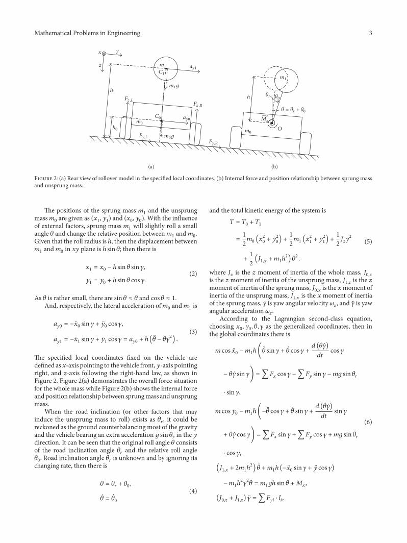
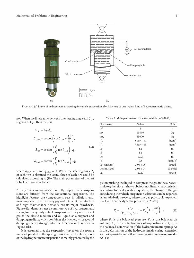

Hindawiwwwhindawicom Volume 2018
MathematicsJournal of
Hindawiwwwhindawicom Volume 2018
Mathematical Problems in Engineering
Applied MathematicsJournal of
Hindawiwwwhindawicom Volume 2018
Probability and StatisticsHindawiwwwhindawicom Volume 2018
Journal of
Hindawiwwwhindawicom Volume 2018
Mathematical PhysicsAdvances in
Complex AnalysisJournal of
Hindawiwwwhindawicom Volume 2018
OptimizationJournal of
Hindawiwwwhindawicom Volume 2018
Hindawiwwwhindawicom Volume 2018
Engineering Mathematics
International Journal of
Hindawiwwwhindawicom Volume 2018
Operations ResearchAdvances in
Journal of
Hindawiwwwhindawicom Volume 2018
Function SpacesAbstract and Applied AnalysisHindawiwwwhindawicom Volume 2018
International Journal of Mathematics and Mathematical Sciences
Hindawiwwwhindawicom Volume 2018
Hindawi Publishing Corporation httpwwwhindawicom Volume 2013Hindawiwwwhindawicom
The Scientific World Journal
Volume 2018
Hindawiwwwhindawicom Volume 2018Volume 2018
Numerical AnalysisNumerical AnalysisNumerical AnalysisNumerical AnalysisNumerical AnalysisNumerical AnalysisNumerical AnalysisNumerical AnalysisNumerical AnalysisNumerical AnalysisNumerical AnalysisNumerical AnalysisAdvances inAdvances in Discrete Dynamics in
Nature and SocietyHindawiwwwhindawicom Volume 2018
Hindawiwwwhindawicom
Dierential EquationsInternational Journal of
Volume 2018
Hindawiwwwhindawicom Volume 2018
Decision SciencesAdvances in
Hindawiwwwhindawicom Volume 2018
AnalysisInternational Journal of
Hindawiwwwhindawicom Volume 2018
Stochastic AnalysisInternational Journal of
Submit your manuscripts atwwwhindawicom