An improved-Rhie-Chow interpolation scheme for the ... · Yi, W., Corbett, D., & Yuan, X-F. (2016). An improved-Rhie-Chow interpolation scheme for the smoothed-interface An improved-Rhie-Chow

The University of Manchester Research

An improved-Rhie-Chow interpolation scheme for thesmoothed-interface immersed boundary methodDOI:10.1002/fld.4240

Document VersionAccepted author manuscript

Link to publication record in Manchester Research Explorer

Citation for published version (APA):Yi, W., Corbett, D., & Yuan, X-F. (2016). An improved-Rhie-Chow interpolation scheme for the smoothed-interfaceimmersed boundary method. International Journal for Numerical Methods in Fluids. https://doi.org/10.1002/fld.4240

Published in:International Journal for Numerical Methods in Fluids

Citing this paperPlease note that where the full-text provided on Manchester Research Explorer is the Author Accepted Manuscriptor Proof version this may differ from the final Published version. If citing, it is advised that you check and use thepublisher's definitive version.

General rightsCopyright and moral rights for the publications made accessible in the Research Explorer are retained by theauthors and/or other copyright owners and it is a condition of accessing publications that users recognise andabide by the legal requirements associated with these rights.

Takedown policyIf you believe that this document breaches copyright please refer to the University of Manchester’s TakedownProcedures [http://man.ac.uk/04Y6Bo] or contact [email protected] providingrelevant details, so we can investigate your claim.

Download date:11. Jan. 2020

https://doi.org/10.1002/fld.4240

https://www.research.manchester.ac.uk/portal/en/publications/an-improvedrhiechow-interpolation-scheme-for-the-smoothedinterface-immersed-boundary-method(7575586c-d30b-424d-95df-f59863546da1).html



https://doi.org/10.1002/fld.4240

Acc

epte

dA

rtic

leAn improved-Rhie-Chow interpolation scheme for the

smoothed-interface immersed boundary method

Wei Yi∗1,2, Daniel Corbett1, Xue-Feng Yuan1,3

1Manchester Institute of Biotechnology, The School of Chemical Engineering and Analytical Science,The University of Manchester, Manchester, United Kingdom

2State key Laboratory of High Performance Computing, The School of Computer,National University of Defense Technology, Changsha, P. R. China

3National Supercomputer Centre in Guangzhou, Research Institute on Application of High Performance Computing,Sun Yat-Sen University, Guangzhou, P. R. China

SUMMARY

Rhie-Chow interpolation is a commonly used method in CFD calculations on a co-located mesh in orderto suppress non-physical pressure oscillations arising from chequer-board effects. A fully parallelisedsmoothed-interface immersed boundary method on a co-located grid is described in this paper. We discussthe necessity of modifications proposed by Choi [1] to the original Rhie-Chow interpolation in order to dealwith a locally refined mesh. Numerical simulation with the modified scheme of Choi shows that numericaldissipation due to Rhie-Chow interpolation introduces significant errors at the immersed boundary. Toaddress this issue we develop an improved-Rhie-Chow interpolation scheme which is shown to increasethe accuracy in resolving the flow near the immersed boundary. We compare our improved scheme with themodified scheme of Choi by parallel simulations of benchmark flows i/ flow past a stationary cylinder, ii/flow past an oscillating cylinder and iii/ flow past a stationary elliptical cylinder, where Reynolds numbers aretested in the range 10 - 200. Our improved scheme is significantly more accurate and compares favourablywith a staggered grid algorithm. We also develop a scheme to compute the boundary force for the direct-forcing immersed boundary method efficiently. Copyright c© 2016 John Wiley & Sons, Ltd.

Received . . .

KEY WORDS: Rhie-Chow interpolation; immersed boundary method; OpenFOAM; finite volumemethod

∗Correspondence to: State key Laboratory of High Performance Computing, The School of Computer, NationalUniversity of Defense Technology, Changsha, P. R. China, Tel: +86-13564101298 Email:[email protected]

This article has been accepted for publication and undergone full peer review but has notbeen through the copyediting, typesetting, pagination and proofreading process, whichmay lead to differences between this version and the Version of Record. Please cite thisarticle as doi: 10.1002/fld.4240

This article is protected by copyright. All rights reserved.

Acc

epte

dA

rtic

le2 W. YI, D. CORBETT AND X.-F. YUAN

1. INTRODUCTION

For the simulation of fluid flow with moving objects of complex geometry, a conventional methodis to dynamically update the mesh according to the new positions of the moving objects, which isreferred as remeshing. The dynamic mesh method has the advantage of a well-controlled accuracy inenforcing the boundary condition on the surfaces of moving objects at an expensive computationalcost. An alternative method without such expensive remeshing procedure is the immersed boundarymethod, where moving objects are tracked by a moving Lagrangian grid while the fluid flow issolved on a stationary Cartesian grid. It is especially favorable for simulating fluid flow with multiplemoving objects and in parallel computing.

The immersed boundary method can be categorized as smoothed-interface immersed boundarymethod, where the boundary is smeared out, or the sharp-interface immersed boundary method.The former is usually first-order accurate in space for flow near a sharp boundary while the lattercan be second-order or higher. The original immersed boundary method belongs to the smoothedcategory. It was proposed by Peskin [2] for simulating blood flow around heart valves. Exchanginginformation between the Lagrangian and Eulerian grids is through a smoothed delta function so theflow field is smeared out in the vicinity of the immersed boundary. Smoothed delta functions [3]should follow fundamental principles, such as momentum conservation, torque conservation etc.An immersed boundary is accomplished by imposing a boundary force, which is introduced intothe momentum equation in a way similar to a body force. The boundary force on Lagrangian pointscan be obtained by solving a constitutive model (Hookean spring [2]), a feedback force model[4] or using the direct forcing method [5]. The direct forcing method has recently gained morepopularity [6, 7, 8, 9] because it requires no additional parameters and is suitable for problems withrigid immersed objects. However, due to the use of a smoothed delta function, the flow at a sharpinterface is difficult to resolve. The sharp-interface immersed boundary method is favored whenboundary layer effects are significant to the entire flow domain, especially for turbulent flow. Thismethod usually involves a local reconstruction of velocity and pressure at the grid near the immersedboundary. It has been widely used in simulating flow with relatively high Reynolds number[10, 11, 12, 13, 14]. Second-order accuracy has been achieved at the fluid-solid interface. Howeverthere are also problems which restrict its application. The local reconstruction performed by linear,bi-linear or quadratic interpolation [10, 11] cannot guarantee mass conservation. Additionally, witha moving boundary on top of a Cartesian grid, physical variables in a Cartesian cell can suddenlytransit between the solid phase and the fluid phase, leading to serious spurious oscillations [15, 16]in the pressure field. These spurious oscillations can be attenuated by a field extension strategywith some ghost cells inside the immersed object [12] and the mass conservation can be improvedby using a more delicate mesh to resolve the geometry of the boundary with cut-cell techniques[17, 18]. In comparison, the oscillation is much less significant with a smoothed-interface immersedboundary method for the simulation of moving boundary problems [6, 19].

Reviewing previous implementations of immersed boundary methods, we find that staggeredgrids has been chosen in most cases. The co-located grid method is widely-known to be vulnerableto the chequer-board effect where nonphysical pressure oscillations appear. Udaykumar et al. [17]proposed a co-located sharp-interface immersed boundary method with an improved Rhie-Chowinterpolation. Mittal et al. [13] also implemented a sharp-interface immersed boundary method on


Acc

epte

dA

rtic

le A CO-LOCATED SMOOTHED-INTERFACE IMMERSED BOUNDARY METHOD 3

a co-located grid. The Mittal group calculated the surface flux by directly taking into account thepressure gradient on cell-faces. Their method can be regarded as a simplified version of the originalRhie-Chow interpolation [20] considering only the diagonal coefficients from the temporal termbut without the implicit viscous term in the momentum equation. Therefore nonphysical pressureoscillation could still appear when the viscous implicit terms dominate. The investigation of asmoothed-interface immersed boundary method on a co-located mesh was not found in literatures.With the original Rhie-Chow interpolation, Choi found that the steady state solution was dependenton the time step, Yu et al. [21] suggested that the chequer-board effect would still appear if a smalltime step is used. A modification was proposed to address this issue by considering a separatetreatment of the temporal term in the interpolation [1, 21]. A general summary of the Rhie-Chowinterpolation can be found in [22].

In this paper we will discuss several issues related to the implementation of a co-locatedsmoothed-interface immersed boundary solver. Major contributions of this paper include:

(i) We develop a numerical method for a smoothed-interface immersed boundary method with animproved-Rhie-Chow interpolation scheme. To our knowledge, this is the first of such schemewhich uses a co-located grid.

(ii) The accuracy of enforcing the no-slip boundary condition at the immersed boundary istypically increased by either using more forcing iterations or decreasing the time step (orboth) [8, 23]. We develop a more cost-effective scheme by adopting an initial estimate forthe boundary force based on its value in the previous time step. We validate our new schemeagainst benchmark flows.

(iii) We have analysed the error introduced by the original Rhie-Chow interpolation and themodified Rhie-Chow interpolation [1]. The latter is necessary when dealing with locallyrefined meshes. Various types of Rhie-Chow interpolation is found to produce significantnumerical dissipation near an immersed boundary where the pressure is discontinuous[24, 25]. We develop an improved-Rhie-Chow algorithm which significantly reducesthe dissipation close to the immersed boundary. We compare our improved-Rhie-Chowinterpolation with Choi’s modified version in two benchmark simulations and demonstrateour method is able to resolve flows near the immersed boundary at higher accuracy.

(iv) Our algorithms are developed in OpenFOAM, an open-source finite volume method (FVM)solver written in C++. OpenFOAM provides many data-structures particularly suited for CFDcalculations (vectors, 2nd rank tensors...) and also makes parallelisation of algorithms simpleand efficient.

2. NUMERICAL METHOD

2.1. Momentum equation discretization

The motion of an incompressible fluid flow is governed by the momentum equation and thecontinuity equation, written as

∂tu+ u · ∇u = −∇p+η

ρf∇2u+ f (1)


Acc

epte

dA

rtic


∇ · u = 0 (2)

where η is the dynamic viscosity of the fluid, ρf is the density of the fluid, p is the kinematicpressure, ∂t indicates a partial derivative with respect to time, f is the boundary force (per unitmass) in the vicinity of the immersed boundary. The force density f is described in section 2.3.

The convection term is discretized with the second-order Adam-Bashforth scheme. The diffusionterm and the boundary force term are discretized with the second-order Crank-Nicholson scheme.Thus the overall accuracy of the numerical scheme is second-order in time.

un+1 − un

∆t= −3

2C[un] +

1

2C[un−1] +

η

2ρf(∇2un +∇2un+1)−∇pn+ 1

2 +1

2(fn + fn+1) (3)

where C is the convection operator and the superscript indicates the time step.The momentum equation is solved with a co-located finite volume method. The integral of the

momentum equation in a control volume involves the computation of several face-centre quantitiesfrom cell-centre variables, including face-centre velocity, flux, face-centre gradient and face-centregradient along the normal direction. The face-centre velocity is obtained by mid-point interpolationfrom the cell-centre velocity. The face-centre gradient is computed with a second-order centraldifference scheme. Rhie-Chow interpolation is used for computing the flux in order to avoid thewell-known chequer-board effect (see section 2.4). In the presence of a local refined mesh, anover-relaxed non-orthogonal correction [26] is chosen to correct the error in gradient at interfacesbetween the coarse and the refined mesh grid, where the connection between cell centres are notaligned with the face normal.

The discretized momentum equation can be reformulated as follows:

aPun+1P = HP − (∇p)P +

unP∆t

(4)

where aP is the diagonal coefficient of the linear equations, unP /∆t is the explicit part of the timederivative term ∂tuP , HP is a combination of implicit off-diagonal terms, other explicit terms andsource terms of the momentum equation.

2.2. Immersed boundary method

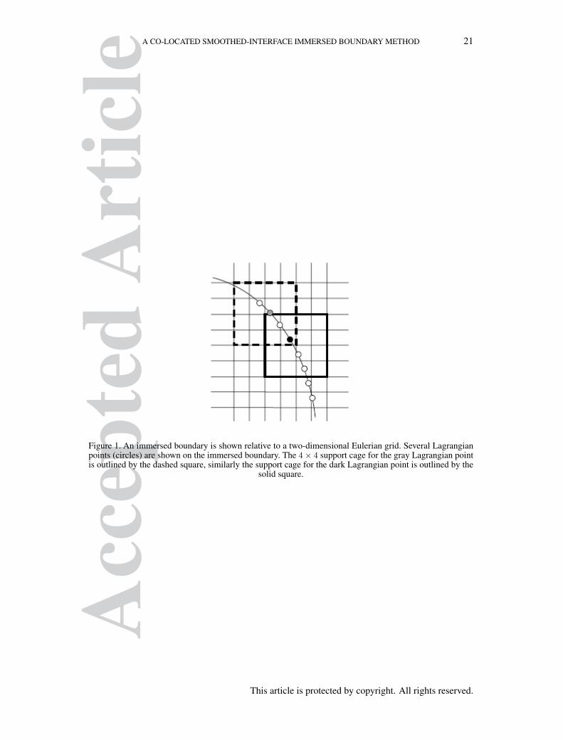
The immersed boundary method uses a separate Lagrangian mesh to track the surface of immersedobjects. Figure 1 shows an immersed boundary (circle points) on a uniform Eulerian grid. Theboundary condition can be enforced by boundary forces on Lagrangian points. The Lagrangianforce is spread to nearby Eulerian grid inside a support cage (e.g. the 4× 4 dashed square in Figure 1for the gray circular Lagrangian point). The Navier-Stokes equation is solved on the Eulerian gridwith the finite volume method. Information exchange between the Eulerian and Lagrangian gridgenerally consists of two steps: one step is to calculate the velocity of the Lagrangian points by aninterpolation from the velocity of the Eulerian points; the other step is to spread the aforementionedforce from Lagrangian points to the Eulerian points in their support cages. For clarity, the variablesfor Lagrangian points are denoted by capital letters, e.g. the boundary force F and the Lagrangianvelocity U . The boundary force (per unit mass) on Eulerian points (achieved by spreading) isintroduced to the momentum equation as a source term f , as shown in eqns. 1 and 3. The size


Acc

epte

dA

rtic


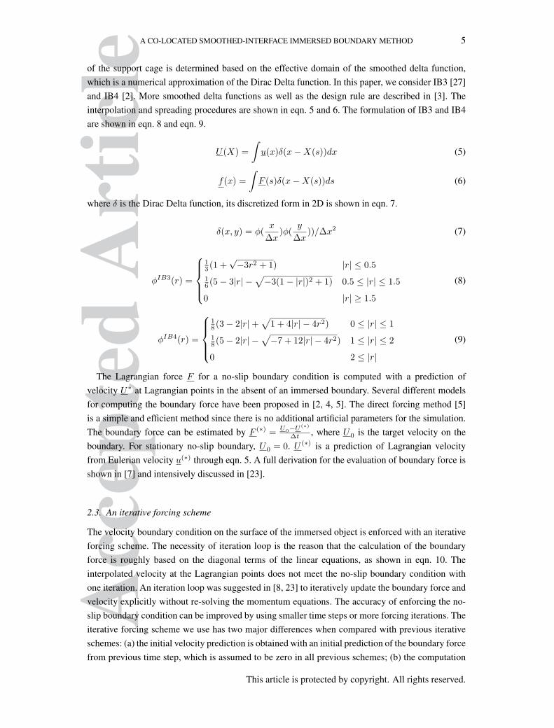
of the support cage is determined based on the effective domain of the smoothed delta function,which is a numerical approximation of the Dirac Delta function. In this paper, we consider IB3 [27]and IB4 [2]. More smoothed delta functions as well as the design rule are described in [3]. Theinterpolation and spreading procedures are shown in eqn. 5 and 6. The formulation of IB3 and IB4are shown in eqn. 8 and eqn. 9.

U(X) =

∫u(x)δ(x−X(s))dx (5)

f(x) =

∫F (s)δ(x−X(s))ds (6)

where δ is the Dirac Delta function, its discretized form in 2D is shown in eqn. 7.

δ(x, y) = φ(x

∆x)φ(

y

∆x))/∆x2 (7)

φIB3(r) =

13 (1 +

√−3r2 + 1) |r| ≤ 0.5

16 (5− 3|r| −

√−3(1− |r|)2 + 1) 0.5 ≤ |r| ≤ 1.5

0 |r| ≥ 1.5

(8)

φIB4(r) =

18 (3− 2|r|+

√1 + 4|r| − 4r2) 0 ≤ |r| ≤ 1

18 (5− 2|r| −

√−7 + 12|r| − 4r2) 1 ≤ |r| ≤ 2

0 2 ≤ |r|

(9)

The Lagrangian force F for a no-slip boundary condition is computed with a prediction ofvelocity U∗ at Lagrangian points in the absent of an immersed boundary. Several different modelsfor computing the boundary force have been proposed in [2, 4, 5]. The direct forcing method [5]is a simple and efficient method since there is no additional artificial parameters for the simulation.The boundary force can be estimated by F (∗) =

U0−U(∗)

∆t , where U0 is the target velocity on theboundary. For stationary no-slip boundary, U0 = 0. U (∗) is a prediction of Lagrangian velocityfrom Eulerian velocity u(∗) through eqn. 5. A full derivation for the evaluation of boundary force isshown in [7] and intensively discussed in [23].

2.3. An iterative forcing scheme

The velocity boundary condition on the surface of the immersed object is enforced with an iterativeforcing scheme. The necessity of iteration loop is the reason that the calculation of the boundaryforce is roughly based on the diagonal terms of the linear equations, as shown in eqn. 10. Theinterpolated velocity at the Lagrangian points does not meet the no-slip boundary condition withone iteration. An iteration loop was suggested in [8, 23] to iteratively update the boundary force andvelocity explicitly without re-solving the momentum equations. The accuracy of enforcing the no-slip boundary condition can be improved by using smaller time steps or more forcing iterations. Theiterative forcing scheme we use has two major differences when compared with previous iterativeschemes: (a) the initial velocity prediction is obtained with an initial prediction of the boundary forcefrom previous time step, which is assumed to be zero in all previous schemes; (b) the computation


Acc

epte

dA

rtic


of boundary force on the Lagrangian points is done according to eqn. 11 based on the diagonalcoefficient of the linear equations (eqn. 4). The difference from the treatment of forcing with eqn. 10and 11 vanishes as the time step reduces. No significant difference is shown when simulation resultsfrom the two formulations are compared.

At the beginning of each time iteration, the velocity is predicted by solving the momentumequation with a fully-explicit scheme, shown in eqn. 12.

F ′ =U0 − U

∗

∆t(10)

F ′ = ap(U0 − U∗) (11)

where ap is the diagonal coefficient of the linear equations.

un+1 − un

∆t= −3

2C[un] +

1

2C[un−1] +

η

ρf∇2un −∇pn + fn (12)

The algorithm for the iterative forcing procedure is summarized in the following six steps:step 0: nIter = 0;step 1: use the force on Lagrangian points from the previous time step with F ∗ = Fn, and spread

F ∗ to Eulerian grid f∗ according to eqn. 6;step 2: solve the momentum equation explicitly with eqn. 12 to get a prediction of the velocity

field u∗;step 3: interpolate the velocity from the Eulerian grid u∗ to the Lagrangian grid U∗ with eqn. 5;step 4: evaluate the boundary force correction F ′ with eqn. 11 and update the boundary force

F ∗ = F ∗ + F ′;step 5: solve the momentum equation implicitly with eqn. 3;step 6: nIter = nIter + 1, if nIter < forceIter return to step 3.It is worth mentioning that although the pressure correction procedure after solving the

momentum equation makes changes to the velocity field and therefore affects the accuracy forenforcing the no-slip boundary condition. The changes associated with the pressure correctionprocedure are insignificant and negligible.

2.4. Rhie-Chow interpolation

2.4.1. original scheme Consider the discretization of the momentum equation onto a uniform gridin the form of eqn. 4 for the cell P and its east neighbour E with face e between them,

aPun+1P = HP − (∇p)P +

unP∆t

(13)

aEun+1E = HE − (∇p)E +

unE∆t

(14)

The Rhie-Chow interpolation proposed by Rhie and Chow [20] computes the face-centre velocityas follows,

aeun+1e = (HE +HP )/2− (∇p)e +

(unP + unE)

2∆t(15)


Acc

epte

dA

rtic


where ae = aP = aE for a uniform grid and (∇p)e = (pE − pP )/∆x, notice (∇p)e 6=12 [(∇p)P + (∇p)E ].

Consider the 1D case,∇p is replaced by ∂p∂x . We can obtain the following equation from eqns. 13,

14 and 15,

un+1e =

1

2(un+1P + un+1

E )− 1

ae

[(∂p

∂x

)e

− 1

2

(∂p

∂x

)P

− 1

2

(∂p

∂x

)E

](16)

According to the Taylor series expansions, the Rhie-Chow interpolation introduces a third-orderderivative term of the pressure in space to the velocity as follows,(

∂p

∂x

)e

− 1

2

(∂p

∂x

)P

− 1

2

(∂p

∂x

)E

= −∆x2

8

(∂3p

∂x3

)e

+O(∆x4) (17)

When the viscous term in the momentum equation is discretised explicitly, ae = ρ/∆t. As a result,eqn. 16 becomes,

un+1e =

1

2(un+1P + un+1

E ) +∆x2

8

∆t

ρ

(∂3p

∂x3

)e

(18)

In our numerical implementation, we calculate the flux based in the absence of the pressurecontribution as follows,

aeu∗e = (HE +HP )/2 +

(unP + unE)

2∆t(19)

The pressure field can then be solved with the following equation,

1

aP∇2p = ∇ · u∗ (20)

The cell-centre velocity field is then updated with the pressure field according to,

un+1 = u∗ − ∇paP

(21)

It can be proved that solving the pressure with eqns. 19 and 20 is equivalent to the original Rhie-Chow interpolation where a correction of pressure is solved together with eqn. 15.

We summarise the pressure correction algorithm in the following,step 0: nIter=0;step 1: calculate the flux with eqn. 19, note the operator H involving implicit terms from

neighbouring cells is also updated;step 2: solve the pressure with eqn. 20 and update the velocity field un+1 with eqn. 21;step 3: nIter = nIter + 1, if nIter < pressureIter return to step 1.

2.4.2. modified-Rhie-Chow interpolation scheme A modified-Rhie-Chow scheme was suggestedin [1, 21] because the original scheme was found to have some weak points: (a) the steady statesolution depends on the time step length [1], (b) chequer-board effects still appear if a small timestep is used [21]. A remedy was introduced considering a separate treatment of the temporal termin the interpolation [1, 21] shown below,


Acc

epte

dA

rtic


aeun+1e = (HE +HP )/2− (∇p)e +

une∆t

(22)

where une is the face-centre velocity calculated in previous time step. In practice, the flux at old timestep is stored rather than the face-centre velocity for the convenience of implementation.

We again analyse error terms using the 1D case. From eqns. 13, 14 and 25, the modified-Rhie-Chow interpolation can be described by,

un+1e =

1

2(un+1P + un+1

E )− 1

ae

[(∂p

∂x

)e

− 1

2

(∂p

∂x

)P

− 1

2

(∂p

∂x

)E

]+une∆t− (unP + unE)

2∆t(23)

Sinceune∆t− (unP + unE)

2∆t= −∆x2

8∆t

(∂2u

∂x2

)e

+O(∆x4/∆t) (24)

The modified Rhie-Chow interpolation introduces an additional second-order derivative term of thevelocity in space to the velocity as follows,

un+1e =

1

2(unP + unE) +

∆x2

8

∆t

ρ

(∂3p

∂x3

)e

+∆x2

8∆t

(∂2u

∂x2

)e

+O(∆x4) (25)

E1 and E2 are used to represent the two dissipation terms,

E1 =∆x2

8

∆t

ρ

(∂3p

∂x3

)e

(26)

E2 =∆x2

8∆t

(∂2u

∂x2

)e

(27)

With a small time step, E1 vanishes while E2 becomes significant. E1 and E2 could introducelarge errors when the flow field is discontinuous. In addition, the modified Rhie-Chow interpolationintroduces a fourth-order derivative term of pressure and third-order derivative term term of velocityinto the continuity equation.

2.4.3. improved-Rhie-Chow interpolation scheme at the immersed boundary In the conventionalcomputing with a body-fitted mesh, Rhie-Chow interpolation is not applied for computing the fluxat boundaries because the flux can be achieved based on the boundary conditions. With an immersedboundary method, the internal part of the immersed boundary also participate in solving theNavier-Stokes equations. Due to the enforcing of the no-slip boundary condition with a smoothedboundary force, the pressure field in the vicinity of the immersed surface becomes nonphysicaland a discontinuity in the pressure is present even with a staggered grid method (Figure 5 in [7]).Therefore, the discontinuity in pressure should also be maintained for a co-located grid method.However, the numerical dissipation in eqn. 18 involves a third-order derivative of pressure in space.Due to the discontinuity in pressure, the numerical dissipation is large and would have a much moresignificant impact on the face-centre velocity in comparison to a smooth pressure field. The Rhie-Chow interpolation tends to smooth the pressure profile near the immersed boundary. It is interestingto investigate the effect of Rhie-Chow interpolation in the vicinity of an immersed boundary wherea boundary force is present. We developed a numerical solver avoiding Rhie-Chow interpolation at


Acc

epte

dA

rtic


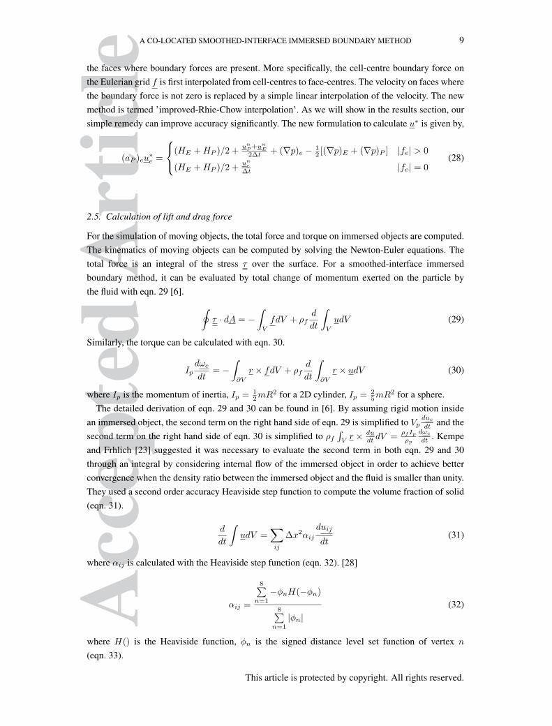
the faces where boundary forces are present. More specifically, the cell-centre boundary force onthe Eulerian grid f is first interpolated from cell-centres to face-centres. The velocity on faces wherethe boundary force is not zero is replaced by a simple linear interpolation of the velocity. The newmethod is termed ’improved-Rhie-Chow interpolation’. As we will show in the results section, oursimple remedy can improve accuracy significantly. The new formulation to calculate u∗ is given by,

(aP )eu∗e =

(HE +HP )/2 +unP +un

E

2∆t + (∇p)e − 12 [(∇p)E + (∇p)P ] |fe| > 0

(HE +HP )/2 +une

∆t |fe| = 0(28)

2.5. Calculation of lift and drag force

For the simulation of moving objects, the total force and torque on immersed objects are computed.The kinematics of moving objects can be computed by solving the Newton-Euler equations. Thetotal force is an integral of the stress τ over the surface. For a smoothed-interface immersedboundary method, it can be evaluated by total change of momentum exerted on the particle bythe fluid with eqn. 29 [6]. ∮

τ · dA = −∫V

fdV + ρfd

dt

∫V

udV (29)

Similarly, the torque can be calculated with eqn. 30.

Ipdωc

dt= −

∫∂V

r × fdV + ρfd

dt

∫∂V

r × udV (30)

where Ip is the momentum of inertia, Ip = 12mR

2 for a 2D cylinder, Ip = 25mR

2 for a sphere.The detailed derivation of eqn. 29 and 30 can be found in [6]. By assuming rigid motion inside

an immersed object, the second term on the right hand side of eqn. 29 is simplified to Vpduc

dt and thesecond term on the right hand side of eqn. 30 is simplified to ρf

∫Vr × du

dt dV =ρf Ipρp

dωc

dt . Kempeand Frhlich [23] suggested it was necessary to evaluate the second term in both eqn. 29 and 30through an integral by considering internal flow of the immersed object in order to achieve betterconvergence when the density ratio between the immersed object and the fluid is smaller than unity.They used a second order accuracy Heaviside step function to compute the volume fraction of solid(eqn. 31).

d

dt

∫udV =

∑ij

∆x2αijduij

dt(31)

where αij is calculated with the Heaviside step function (eqn. 32). [28]

αij =

8∑n=1

−φnH(−φn)

8∑n=1

|φn|(32)

where H() is the Heaviside function, φn is the signed distance level set function of vertex n

(eqn. 33).


Acc

epte

dA

rtic


φn = |xijn − xc| −R (33)

where xijn is the position vector of the nth vertex of the grid cell, and xc is the position vector ofthe mass centre, R is the radius.

2.6. Boundary conditions

2.6.1. Dirichlet boundary condition When a Dirichlet boundary condition is applied on a boundary,evaluation of surface gradient (snGrad) along the normal direction is discretized by a one-sided scheme (OpenFOAM 2.3.1), as is shown in eqn. 34. snGrad is required for finite-volumediscretization of the viscous term in the momentum equation.

u′ =ue − uP∆x/2

(34)

This scheme is first-order accurate for the evaluation of the gradient.

ue = uP +∆x

2u′P +

∆x2

4

1

2u′′P +

∆x3

8

1

6u′′′P +O(∆x4) (35)

uW = uP −∆xu′P +1

2∆x2u′′P −

1

6∆x3u′′′P +O(∆x4) (36)

[2× ( 35) + (36)]/∆x2

2(ue − uP )/∆x− (uP − uW )/∆x

∆x=

3

4u′′P −

1

8∆xu′′′P +O(∆x2) (37)

[ 83 × ( 35)− 4

3 × (36)]/∆x2

83ue − 4uP + 4

3uW

∆x2= u′′P −

1

6∆xu′′′P +O(∆x2) (38)

u′e =83ue − 3uP + 1

3uW

∆x+O(∆x2) (39)

The Taylor expansion shows the error for Laplacian term in original scheme for handling Dirichletboundary is O(1) (eqn. 37). However, the scheme can be easily improved by a correction coefficient(eqn. 38). The corresponding equation for evaluation of snGrad at the Dirichlet boundary is shownin eqn. 39 with a second-order accuracy in space.

2.6.2. Neumann boundary condition A Neumann boundary condition specifies the gradient alongthe normal direction. The evaluation of variables on face centres is necessary for the finite-volumediscretization of the convection term in the momentum equation. In OpenFOAM 2.3.1, it is alsoimplemented by a one-sided scheme (eqn. 40).

ue ≈ uP +∆x

2u′e (40)


Acc

epte

dA

rtic


ue = uP +∆x

2u′e −

∆x2

8u′′e +O(∆x3) (41)

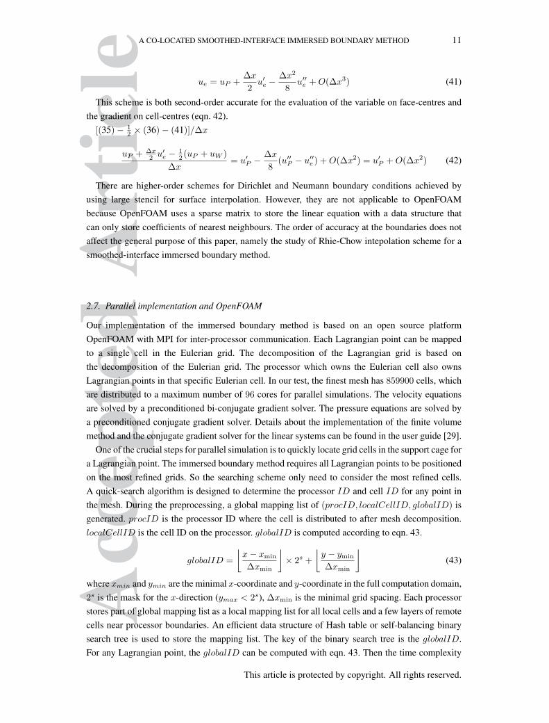
This scheme is both second-order accurate for the evaluation of the variable on face-centres andthe gradient on cell-centres (eqn. 42).

[(35)− 12 × (36)− (41)]/∆x

uP + ∆x2 u′e − 1

2 (uP + uW )

∆x= u′P −

∆x

8(u′′P − u′′e ) +O(∆x2) = u′P +O(∆x2) (42)

There are higher-order schemes for Dirichlet and Neumann boundary conditions achieved byusing large stencil for surface interpolation. However, they are not applicable to OpenFOAMbecause OpenFOAM uses a sparse matrix to store the linear equation with a data structure thatcan only store coefficients of nearest neighbours. The order of accuracy at the boundaries does notaffect the general purpose of this paper, namely the study of Rhie-Chow intepolation scheme for asmoothed-interface immersed boundary method.

2.7. Parallel implementation and OpenFOAM

Our implementation of the immersed boundary method is based on an open source platformOpenFOAM with MPI for inter-processor communication. Each Lagrangian point can be mappedto a single cell in the Eulerian grid. The decomposition of the Lagrangian grid is based onthe decomposition of the Eulerian grid. The processor which owns the Eulerian cell also ownsLagrangian points in that specific Eulerian cell. In our test, the finest mesh has 859900 cells, whichare distributed to a maximum number of 96 cores for parallel simulations. The velocity equationsare solved by a preconditioned bi-conjugate gradient solver. The pressure equations are solved bya preconditioned conjugate gradient solver. Details about the implementation of the finite volumemethod and the conjugate gradient solver for the linear systems can be found in the user guide [29].

One of the crucial steps for parallel simulation is to quickly locate grid cells in the support cage fora Lagrangian point. The immersed boundary method requires all Lagrangian points to be positionedon the most refined grids. So the searching scheme only need to consider the most refined cells.A quick-search algorithm is designed to determine the processor ID and cell ID for any point inthe mesh. During the preprocessing, a global mapping list of (procID, localCellID, globalID) isgenerated. procID is the processor ID where the cell is distributed to after mesh decomposition.localCellID is the cell ID on the processor. globalID is computed according to eqn. 43.

globalID =

⌊x− xmin

∆xmin

⌋× 2s +

⌊y − ymin

∆xmin

⌋(43)

where xmin and ymin are the minimal x-coordinate and y-coordinate in the full computation domain,2s is the mask for the x-direction (ymax < 2s), ∆xmin is the minimal grid spacing. Each processorstores part of global mapping list as a local mapping list for all local cells and a few layers of remotecells near processor boundaries. An efficient data structure of Hash table or self-balancing binarysearch tree is used to store the mapping list. The key of the binary search tree is the globalID.For any Lagrangian point, the globalID can be computed with eqn. 43. Then the time complexity


Acc

epte

dA

rtic


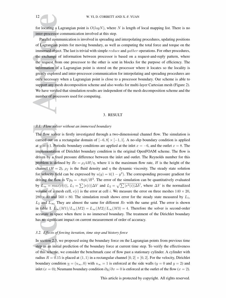
for locating a Lagrangian point is O(logN), where N is length of local mapping list. There is nointer-processor communication involved at this step.

Parallel communication is involved in spreading and interpolating procedures, updating positionsof Lagrangian points for moving boundary, as well as computing the total force and torque on theimmersed object. The last is trivial with simple reduce and gather operations. For other procedures,the exchange of information between processor is based on a request-and-reply pattern, wherethe request from one processor to the other is sent in blocks for the purpose of efficiency. Theinformation of a Lagrangian point is stored on the processor where it locates so the locality isgreatly explored and inter-processor communication for interpolating and spreading procedures areonly necessary when a Lagrangian point is close to a processor boundary. Our scheme is able tosupport any mesh decomposition scheme and also works for multi-layer Cartesian mesh (Figure 2).We have verified that simulation results are independent of the mesh decomposition scheme and thenumber of processors used for computing.

3. RESULT

3.1. Flow solver without an immersed boundary

The flow solver is firstly investigated through a two-dimensional channel flow. The simulation iscarried out on a rectangular domain of [−6, 8]× [−1, 1]. A no-slip boundary condition is appliedat y = ±1. Periodic boundary conditions are applied at the inlet x = −6, and the outlet x = 8. Theimplementation of Dirichlet boundary condition is the original OpenFOAM scheme. The flow isdriven by a fixed pressure difference between the inlet and outlet. The Reynolds number for thisproblem is defined by Re = ρfuH/η, where u is the maximum flow rate, H is the height of thechannel (H = 2), ρf is the fluid density and η the dynamic viscosity. The steady state solutionfor velocity field can be expressed by u(y) = u(1− y2). The corresponding pressure gradient fordriving the flow is ∇p0 = −8ηu/H2. The error of the simulation can be quantitatively evaluatedby L∞ = max|e(i)|, L1 =

∑|e(i)|∆V and L2 =

√∑|e2(i)|∆V , where ∆V is the normalized

volume of a mesh cell, e(i) is the error at cell i. We measure the error on three meshes 140× 20,280× 40 and 560× 80. The simulation result shows error for the steady state measured by L1,L2 and L∞. They are almost the same for different Re with the same grid. The error is shownin table I. L∞(M1)/L∞(M2) = L∞(M2)/L∞(M3) = 4. Therefore the solver is second-orderaccurate in space when there is no immersed boundary. The treatment of the Dirichlet boundaryhas no significant impact on current measurement of order of accuracy.

3.2. Effects of forcing iteration, time step and history force

In section 2.3, we proposed using the boundary force on the Lagrangian points from previous timestep as an initial prediction of the boundary force at current time step. To verify the effectivenessof this scheme, we consider the benchmark case of flow past a stationary cylinder. A cylinder withradius R = 0.15 is placed at (1, 1) in a rectangular channel [0, 2]× [0, 2]. For the velocity, Dirichletboundary condition u = (u∞, 0) with u∞ = 1 is enforced at the side walls (y = 0 and y = 2) andinlet (x = 0); Neumann boundary condition ∂u/∂x = 0 is enforced at the outlet of the flow (x = 2).


Acc

epte

dA

rtic


For the pressure, Neumann boundary condition ∂p/∂n = 0 is enforced at the side walls and inlet;Dirichlet boundary condition p = 0 is set at the outlet. The Reynolds number for this case is definedas Re = ρfuD/η, where D is the diameter of the cylinder. The improved-Rhie-Chow interpolationscheme is used for calculating the flux on the surface.

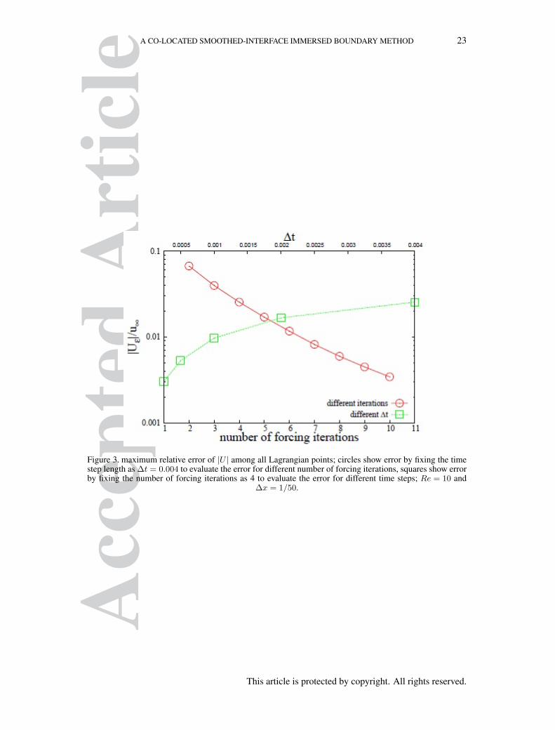
Since the expected velocity on Lagrangian points is zero for a no-slip boundary, the velocity atLagrangian points represents the numerical error. We calculate the velocity at Lagrangian pointswith the smoothed delta function when steady state is reached. For a specific mesh, it is well-understood that this error can be attenuated by increasing the number of forcing iterations or bydecreasing the time step [23]. A uniform grid with grid spacing of 1/50 is used. The Lagrangianpoints are evenly distributed on the surface of the cylinder with ∆s ≈ ∆x, where ∆s is the arclength between two neighbour Lagrangian points, ∆x is the grid spacing. Figure 3 shows the errorof enforcing the no-slip boundary condition. For the study of forcing iteration effect, the time stepis fixed as ∆t = 0.004, with a Courant number at around 0.4; for the study of time step effect, thenumber of forcing iterations is fixed at 4. The number of pressure correction iterations is fixed to 2

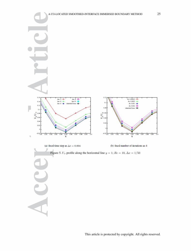
in all simulations in this paper. When the initial prediction of the boundary force is inherited fromforces on Lagrangian points at the previous time step, the error is 10−7 even with 2 forcing iterationsand ∆t = 0.004. Therefore, we think that the prediction from an inherited force can achieve muchhigher accuracy at low computational expense. Figure 4 shows the overall profile of x-componentvelocity, Ux along the centreline when inherited forces are used. Figure 5(a) and 5(b) shows amagnified view of the x-component of velocity near the front of the cylinder without inheritedforces. This figure shows the raw cell-centred data sampled according to the nearest-cell rule. Asthe number of forcing iterations increases or the time step decreases, the velocity profile along thecentre-line approaches the velocity profile predicted with inherited forces. The velocity at the cellsclose to the Lagrangian point appears to be negative. The error at the cells close to the immersedboundary can be further reduced by grid refinement.

3.3. Effect of temporal term in the Rhie-Chow interpolation

The original Rhie-Chow interpolation is able to substantially suppress pressure oscillations dueto the chequer-board effect. As pointed out by Choi [1], for time-dependent simulations, theoriginal Rhie-Chow interpolation results in a steady-state solution that is dependent on the time-step. Additionally, the chequer-board effect still appears if the time step is relative small, i.e. whenthe Courant number is small. The original Rhie-Chow interpolation is likely to cause problemsin simulations with a gradient mesh or a locally refined mesh because the maximum time step islimited by the minimal grid spacing, and local Courant number at the less refined region could bevery small. Local mesh refinement is widely applied in simulation with immersed boundary methoddue to the inherently lower order of accuracy for resolving flow near the boundary. Therefore, thetemporal term (the second term on the r.h.s of eqn. 25) suggested by Choi [1] becomes crucialfor a co-located immersed boundary method. An effective solution is to handle the temporal termseparately in the interpolation (see section 2.4.2). We demonstrate the importance of this temporalterm through a benchmark case running on a local refined mesh.

The benchmark case of flow past a stationary cylinder is again considered to verify the importanceof the temporal correction term in computing face fluxes. The geometry and boundary conditionsare the same as in section 3.2 but in a larger computational domain [0, 16]× [0, 16]. The wall effect


Acc

epte

dA

rtic


on the flow near the cylinder is weak. The cylinder is initially placed at [6.85, 8]. A 4-layer meshis generated as shown in Figure 2. The minimal grid spacing for this test is D/60. The Reynoldsnumber is 40. Nonphysical pressure oscillation is observed to be significant in the coarse meshregion. Figure 6 samples the pressure along the centreline in the range between x = 14 and x = 16.The oscillation of pressure becomes more severe when a smaller time step is used. The effect ofadding a temporal correction term to the original Rhie-Chow interpolation is clearly shown.

3.4. Mesh convergence study of the immersed boundary solver

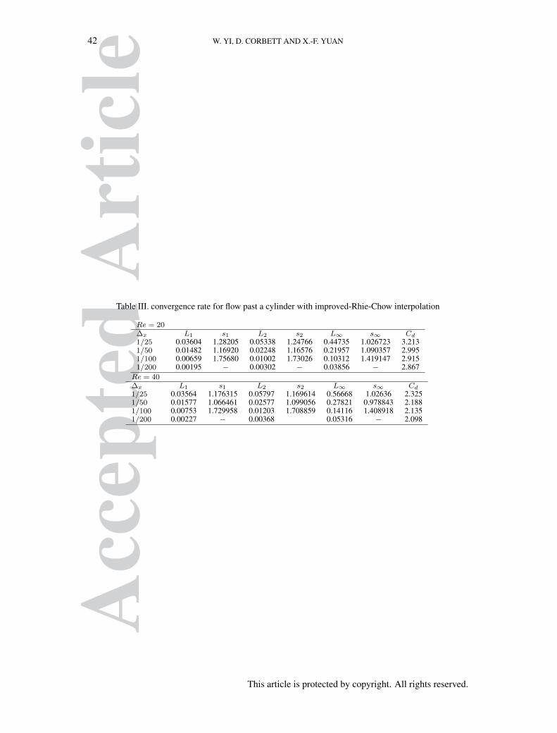
Since there is no analytical solution for the flow, the mesh convergence study uses the simulationresult with a very refined mesh (800× 800) as the reference solution for calculating errors. Theorder of convergence is estimated by s = ln(e(2h)/e(h))/ln2, where e(h) and e(2h) are the errorassociated with meshes of grid spacing h and 2h. The Courant number is kept around 0.4 in allsimulations. Table II and III list the order of convergence in space evaluated on four meshes of size50× 50, 100× 100, 200× 200 and 400× 400. Our measurement of convergence rate is similar tothe simulation carried out in [13, 23]. The reference solution on mesh 800× 800 is interpolatedto coarse meshes with a second-order scheme. The difference between the coarse mesh solutionand the reference solution is calculated and its magnitude represents the error. L1 and L2 areindicators of global accuracy while L∞ demonstrates the error at the immersed boundary. The onlydifference in the solver between the modified- Rhie-Chow interpolation and the improved-Rhie-Chow interpolation is that the latter avoids Rhie-Chow interpolation in the vicinity of the immersedboundary. With the modified-Rhie-Chow interpolation, the order of accuracy is about 1.3 accordingto L1 and L2, but only first-order according to L∞; with the improved-Rhie-Chow interpolation,the order of accuracy is close to first-order according to L∞, L1 and L2. The difference in theorder of convergence between the two solvers reveals that the global error is dominant by the errorintroduced at the immersed boundary. Figure 7(a) and 7(b) show the magnitude of difference inx-direction velocity with mesh 400× 400 and 800× 800 for Re = 40. The improved-Rhie-Chowinterpolation has a better resolution of the flow at the boundary especially less penetration at thefront of the cylinder.

3.5. Flow past a stationary cylinder

To further validate the correctness of our code, we investigate the drag and lift force on a cylinder fordifferent Reynolds number. We use a 4-layer mesh with a computation domain of [0, 16]× [0, 16],the same as in section 3.3. Two different meshes with minimal grid spacing ofD/∆x = 60 (meshA)and D/∆x = 120 (meshB) are considered; the number of Lagrangian points around the cylinderare 192 and 384 respectively. Table IV compares the drag coefficient for Re = 20 and Re = 40.The results show a good consistency with other publications. For larger Re, a Karman vortexstreet is generated at the rear of the cylinder when a small perturbation in the flow is present. Theprediction of the drag and lift coefficients with the improved-Rhie-Chow interpolation shows a betteraccuracy with the same mesh for larger Re even though both methods are likely to converge to asimilar solution if a more refined mesh is used. Figure 9 shows the z-direction vorticity contour forRe = 100 and Re = 200 from simulation with meshB. Figure 8 shows the streamline for different


Acc

epte

dA

rtic


Reynolds numbers. Similar vorticity profiles and streamlines are observed with the modified-Rhie-Chow solver. The corresponding lift and drag coefficient are shown in table V. The drag and liftcoefficients are defined as Cd = Fx/(ρu

2∞R); Cl = Fy/(ρu

2∞R), where Fx and Fy are the drag and

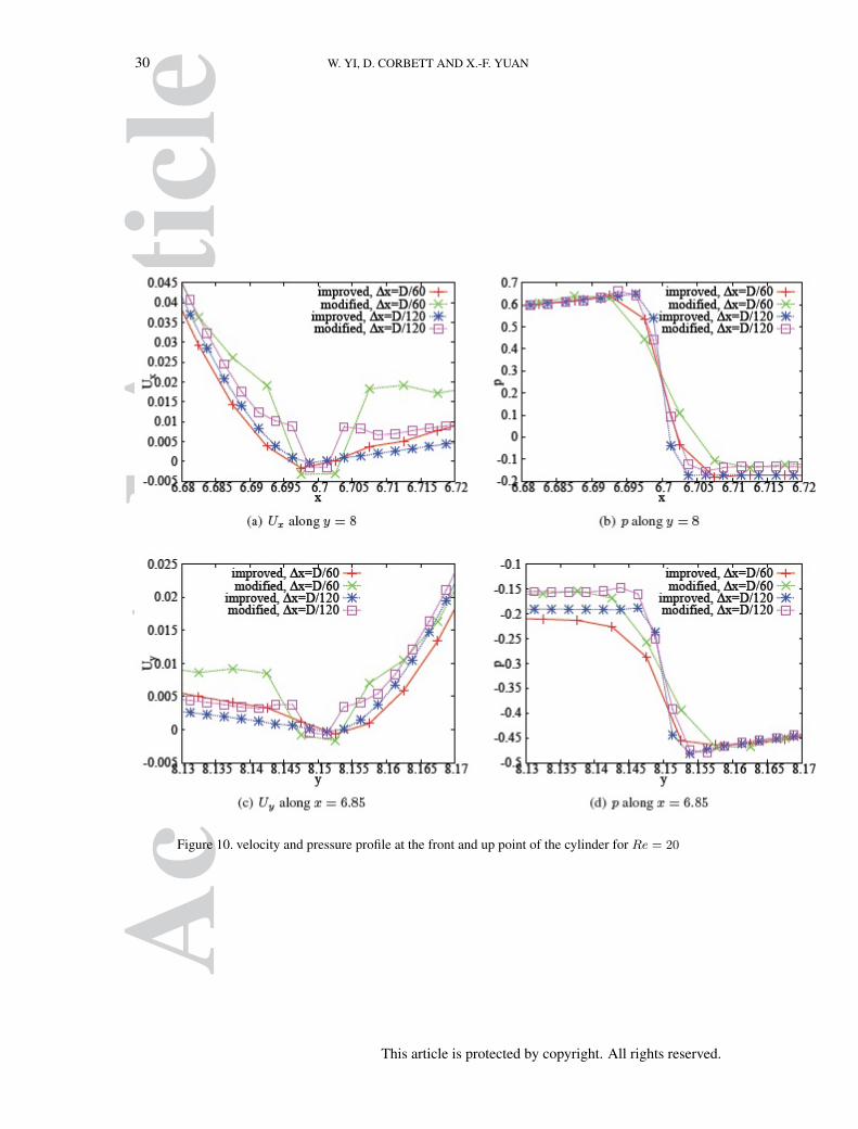
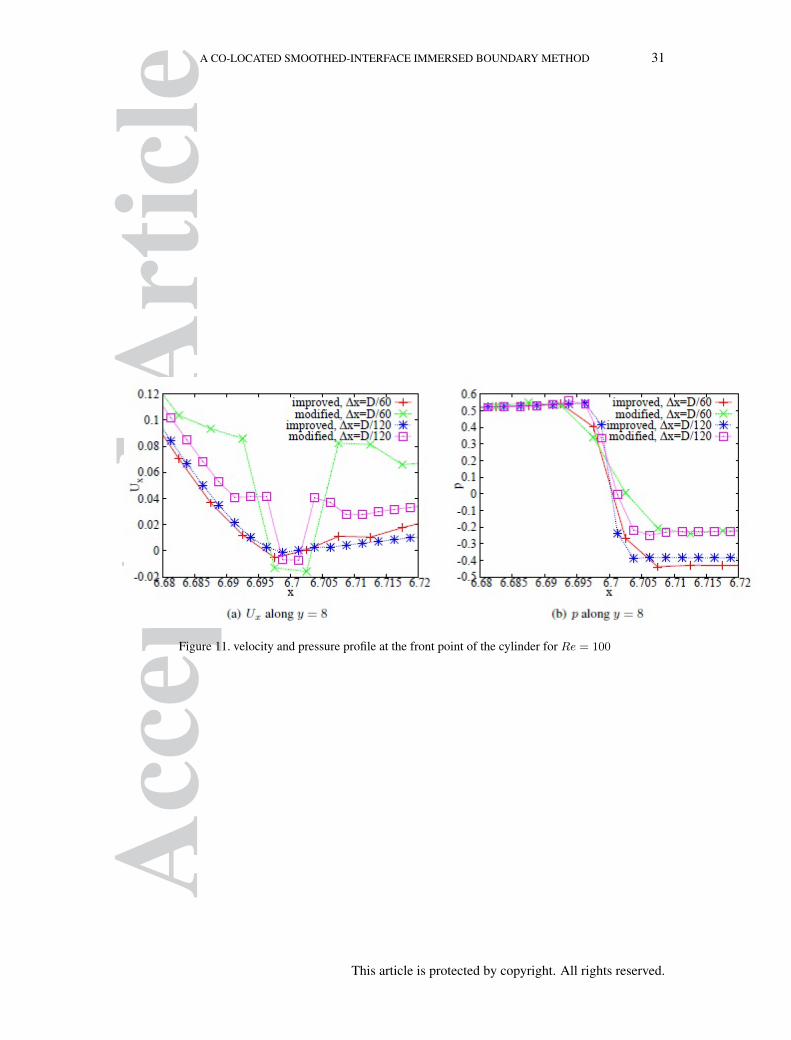
lift force on the cylinder. The Strouhal number is defined as St = fsD/u∞, where fs is the sheddingfrequency of the Karman vortex. Figure 10 compares the velocity and pressure profile at the frontand up point of the cylinder for Re = 20. The velocity from the improved-Rhie-Chow solver issmoother than the modified-Rhie-Chow solver. On the other hand, the pressure from the improved-Rhie-Chow solver is steeper than the modified-Rhie-Chow solver. We also compare velocity andpressure profiles at the front point forRe = 100 (Figure 11). The above results demonstrate superiorpredictions when using the improved-Rhie-Chow interpolation scheme.

3.6. Flow past an oscillatory cylinder

In this part, a benchmark test with a moving boundary is considered. A cylinder in the free streamis moving with a specified periodic oscillation in the direction perpendicular to the cross flow:

y(t) = y0 +A sin(2πfet) (44)

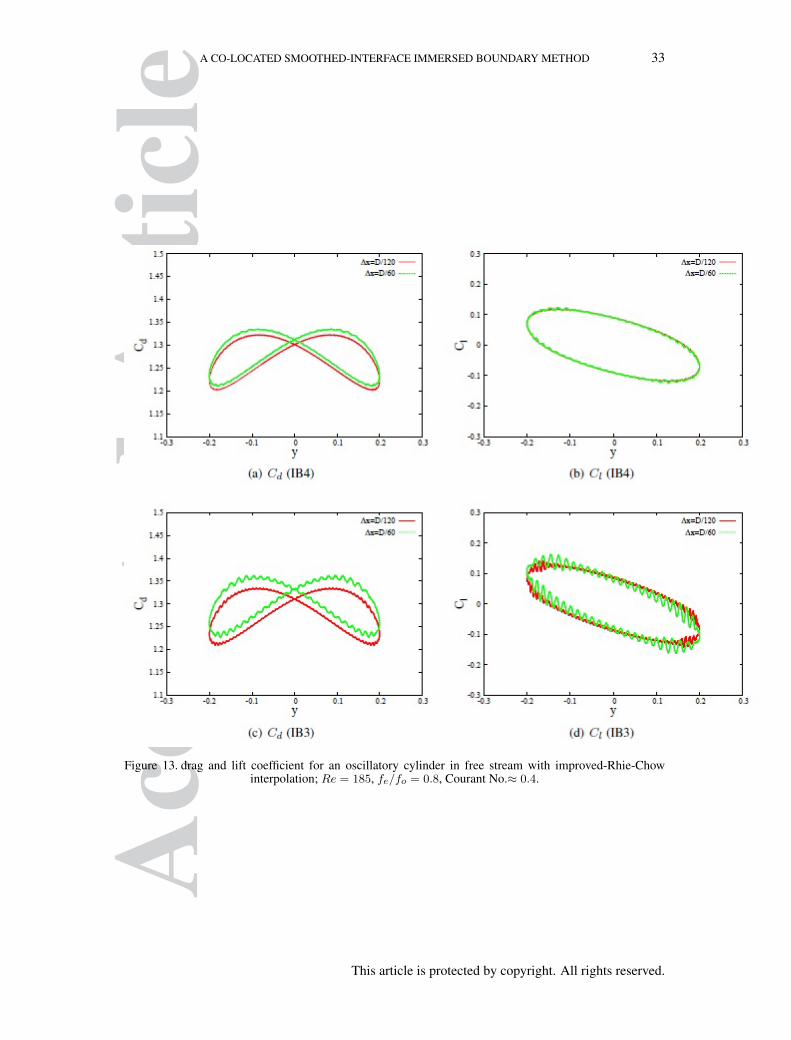
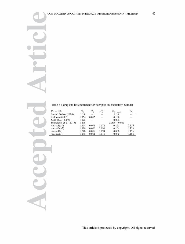
where y(t) is the y-coordinate of the cylinder centre, y0 is the initial y-coordinate,A is the amplitude,fe is the oscillation frequency, A = 0.2D and fe = 0.52. We choose the same Reynolds numberRe = 185 as in [6]. fe is 0.8 times the natural shedding frequency fo at Re = 185. The Courantnumber for all simulations is kept constant at around 0.4. Other configurations are the same as thestationary cylinder case in section 3.5. Table VI shows the simulation result when a pseudo-steadystate is reached. Our improved-Rhie-Chow solver shows similar predictions compared with thatfrom the smoothed-interface immersed boundary method with a staggered grid [19, 36]. MeshA hasa minimal grid spacing of D/60, which is comparable to the grid spacing D/50 used by Yang et al.[19]. The resultant mean drag coefficient and root-mean-square (rms) lift coefficient agree well.In comparison to our improved-Rhie-Chow solver, the modified-Rhie-Chow solver has an over-estimation of drag of 9.5% and 5%, and an over-estimation of the rms lift coefficient of 45.8% and26.8% for meshA and meshB. Figure 12 shows the periodic evolution of the drag and lift coefficientas a function of the y-coordinate with the modified-Rhie-Chow solver. The comparison on twomeshes with grid spacing of D/60 and D/120 shows the prediction of the drag and lift coefficientsare still relatively mesh-dependent. Figure 13 shows the corresponding results with the improved-Rhie-Chow interpolation scheme, the mesh-dependent variation is much smaller. We also carriedout the same simulation with a more compact support cage of 3× 3 grid cells. The selection ofsupport cage has a stronger influence on the modified-Rhie-Chow solver. Figure 12 shows a largererror for the prediction of lift and drag with IB3 than that with IB4. It suggests that the dissipationintroduced by Rhie-Chow interpolation is increased when the pressure profile is less smooth withIB3. Simulation with IB3 with the improved-Rhie-Chow solver does not show a significant changeint the prediction of drag and lift coefficients (Figure 13). The time evolution of Cd and Cl withIB4 is smoother than those with IB3. Comparison between the modified-Rhie-Chow solver andthe improved-Rhie-Chow solver in Figure 12 and Figure 13 show that the improved-Rhie-Chowscheme does not cause stronger oscillations in the drag and lift coefficients. Our improved-Rhie-Chow solver avoids interpolation at surfaces which have a boundary force and we thus conclude


Acc

epte

dA

rtic


that smoothing are not necessary. However, smoothing can easily be incorporated into the solver atan interface where the boundary force is discontinuous across the boundary.

3.7. Flow past a stationary elliptical cylinder

We then consider the case flow past a stationary elliptical cylinder. The equation of an ellipticalcylinder that orients along the flow is given by,

(x− x0)2

a2+

(y − y0)2

b2= 1 (45)

where a and b are the major axis and minor axis. The Lagrangian points are uniformly distributedon the circumference of the cylinder with the same length of arc between neighbouring Lagrangianpoints. The aspect ratio of the eclipse (a/b) is set as 2. The same meshes for the simulation of flowpast a stationary/oscillating cylinder are used, with minimal grid spacings of a/30 and a/60. Themaximum Courant number is kept around 0.3 for all simulations. The Reynolds number for theflow is defined with the major axis of the elliptical cylinder, Re = ρU∞a/ηs. Flow past a stationaryelliptical cylinder with the attack angle of α = 0, π/6, π/3, π/2 are simulated. Figure 14 illustratesstreamlines around the eclipse with different attack angles when Re = 40. When the eclipse orientsalong the flow, the flow is stable with a pair of symmetric vortexes at the rear of the cylinder. As theattack angle increases, flow asymmetry develops and vortexes are generated periodically at the rearof the cylinder. Figure 15 and 16 show the time evolution of drag coefficients when Re = 40 andRe = 100 with different meshes and different interpolation schemes. when the time step decreases,change in the drag profiles is found to be insignificant. The drag coefficient of the elliptical cylinderis defined as Cd = Fd/ρu

2∞a. When the attack angle is π/6 or π/3, the drag profile in a periodic

cycle shows an asymmetric pattern. We can see that the results from the improved-Rhie-Chowinterpolation exhibit a weaker mesh dependency in the drag coefficients, in comparison with thatfrom the modified-Rhie-Chow interpolation. The detailed drag coefficient and the Strouhal numberare described in Table VII and VIII. The Strouhal number is defined as St = 2fsa/u∞, where fs isthe vortex shedding frequency. There is no significant difference for the prediction of the Strouhalnumber between the two schemes (≤ %1). The solver with the improved-Rhie-Chow interpolationis found to give a better prediction for the drag coefficients.

3.8. Sedimentation of a pair of cylinders

The benchmark cases in section 3.5, 3.6 and 3.7 consider either a stationary boundary or a movingboundary with pre-determined motions. In this section, sedimentation of a pair of 2D cylinders issimulated. The translational and angular velocities are solved with the Newton-Euler equations. Thetrailing cylinder accelerates faster due to the drag reduction in the wake area of the leading cylinder,thus approaches the leading cylinder quickly, resulting in a draft-kissing-tumbling pattern. Uhlmann[6] studied the problem with a direct-forcing immersed boundary method on a staggered grid.Simulations of this case with other configurations can be found in [37, 38, 39]. Our study considersthe same parameters as in [6] (table IX). The computational geometry is shown in Figure 17.

To avoid the particle collision due to insufficient grid resolution and to resolve the flow field atthe gap between the particles, an artificial potential force is enforced when the separation between


Acc

epte

dA

rtic


the two cylinders falls below a threshold value [40]. The potential force is given by,

FPi,j =

0 di,j > 2R+ ξP

1εP

(Ci − Cj)(2R+ ξP − di,j) di,j ≤ 2R+ ξP(46)

where Ci and Cj are the position vector of the cylinder centre, di,j is the distance between cylindercentres, ξP is the threshold separation, εp is stiffness. In this test, εp = 5× 10−7 and ξp = 3∆x.

The simulation considers the same grid spacing and time step length used in Uhlmann [6], ∆x =

D/64 and ∆t = 0.0001. The time-evolution of the displacement and the velocity are monitored.The results with the improved-Rhie-Chow interpolation are shown in Figure 18. The x-directiondisplacement and velocity, agree closely with those predicted by Uhlmann [6], up to the stageof “kissing”. In the tumbling stage, the velocity is strongly affected by the parameters set in thecollision model, making it hard to have a qualitatively comparison. In addition, the x-directionvelocity with the modified-Rhie-Chow and the improved-Rhie-Chow interpolations are compared.The predicted x-direction velocity of the leading-cylinder shows a considerable difference with themodified-Rhie-Chow and the improved-Rhie-Chow interpolations even during the drafting periodin the absent of the artificial collision force. Such difference still exists when using a finer mesh,smaller time steps, or more iterations. The x-direction velocity with the improved-Rhie-Chowinterpolation is found to agree with that reported in [6] (Figure 18(b)).

4. CONCLUSION

In this paper we have presented a smoothed-interface immersed boundary method on a co-locatedgrid. Rhie-Chow interpolation is often used for calculating surface fluxes in order to avoid chequer-board effects. However, discontinuities in the pressure field at the immersed boundary result in alarge dissipation from a standard Rhie-Chow interpolation. This dissipation term is the dominatesource of error, and becomes more significant as the Reynolds number increases. We verifiedthis quantitatively by simulating flow past a cylinder. The dissipation could be reduced by meshrefinement at an expensive computational cost. The immersed boundary method with Rhie-Chowinterpolation is far less accurate than a staggered grid method using the same mesh. We thereforehave developed an improved Rhie-Chow interpolation algorithm which uses standard Rhie-Chowinterpolation at surfaces with no boundary force, and avoids interpolation at surfaces with aboundary force. Using this improved Rhie-Chow interpolation with a co-located grid we are able toobtain accuracy matching a staggered grid.

Previous direct forcing immersed boundary methods require a large number of force iterations toaccurately enforce the no-slip boundary condition at the immersed boundary. In this paper we haveused the boundary force from the previous time step as the initial guess for the boundary force at thecurrent time step. Our subsequent simulations confirm that far fewer force iterations are needed toenforce the no-slip boundary condition with this scheme, even if a large time step is used. Finally,our implementation on OpenFOAM provides a readily scalable platform for 3D simulations. Infuture work we intend to apply this method to 3D simulations of hard sphere suspensions.


Acc

epte

dA

rtic


ACKNOWLEDGEMENT

Wei Yi’s PhD studentship is funded by the University of Manchester and the Chinese ScholarshipCouncil. Wei Yi thanks to N8 HPC facility in Leeds and the National supercomputer centre inGuangzhou for providing computing resources. Wei Yi also thanks to the OpenFOAM team inNational University of Defense Technology for helpful discussions.

REFERENCES

[1] Seok Ki Choi. Note on the use of momentum interpolation method for unsteady flows.Numerical Heat Transfer: Part A: Applications, 36(5):545–550, 1999.

[2] Charles S. Peskin. Flow patterns around heart valves: A numerical method. Journal ofComputational Physics, 10(2):252–271, 1972.

[3] Charles S. Peskin. The immersed boundary method. Acta Numerica, 11:479–517, 2002.

[4] D. Goldstein, R. Handler, and L. Sirovich. Modeling a no-slip flow boundary with an externalforce-field. Journal of Computational Physics, 105(2):354–366, 1993. Ku501 Times Cited:269Cited References Count:34.

[5] J. Mohd-Yusof. Combined immersed-boundary/b-spline methods for simulations of flow incomplex geometries. Center for Turbulence Research Annual Research Briefs, pages 317–327, 1997.

[6] Markus Uhlmann. An immersed boundary method with direct forcing for the simulation ofparticulate flows. Journal of Computational Physics, 209(2):448–476, 2005.

[7] A. Pinelli, I. Z. Naqavi, U. Piomelli, and J. Favier. Immersed-boundary methods for generalfinite-difference and finite-volume navierstokes solvers. Journal of Computational Physics,229(24):9073–9091, 2010.

[8] W. P. Breugem. A second-order accurate immersed boundary method for fully resolvedsimulations of particle-laden flows. Journal of Computational Physics, 231(13):4469–4498,2012. 935JU Times Cited:0 Cited References Count:38.

[9] C. Ji, A. Munjiza, and J. J. R. Williams. A novel iterative direct-forcing immersed boundarymethod and its finite volume applications. Journal of Computational Physics, 231(4):1797–1821, 2012.

[10] Yu-Heng Tseng and Joel H. Ferziger. A ghost-cell immersed boundary method for flow incomplex geometry. Journal of Computational Physics, 192(2):593–623, 2003.

[11] Elias Balaras. Modeling complex boundaries using an external force field on fixed cartesiangrids in large-eddy simulations. Computers & Fluids, 33(3):375–404, 2004.


Acc

epte

dA

rtic


[12] Jianming Yang and Elias Balaras. An embedded-boundary formulation for large-eddysimulation of turbulent flows interacting with moving boundaries. Journal of ComputationalPhysics, 215(1):12–40, 2006.

[13] R. Mittal, H. Dong, M. Bozkurttas, F. M. Najjar, A. Vargas, and A. von Loebbecke. Aversatile sharp interface immersed boundary method for incompressible flows with complexboundaries. Journal of Computational Physics, 227(10):4825–4852, 2008.

[14] Jianming Yang and Frederick Stern. A simple and efficient direct forcing immersed boundaryframework for fluidstructure interactions. Journal of Computational Physics, 231(15):5029–5061, 2012.

[15] Jongho Lee, Jungwoo Kim, Haecheon Choi, and Kyung-Soo Yang. Sources of spuriousforce oscillations from an immersed boundary method for moving-body problems. Journalof Computational Physics, 230(7):2677–2695, 2011.

[16] Jung Hee Seo and Rajat Mittal. A sharp-interface immersed boundary method with improvedmass conservation and reduced spurious pressure oscillations. Journal of ComputationalPhysics, 230(19):7347–7363, 2011.

[17] H. S. Udaykumar, Heng-Chuan Kan, Wei Shyy, and Roger Tran-Son-Tay. Multiphasedynamics in arbitrary geometries on fixed cartesian grids. Journal of Computational Physics,137(2):366–405, 1997.

[18] T. Ye, R. Mittal, H. S. Udaykumar, and W. Shyy. An accurate cartesian grid method for viscousincompressible flows with complex immersed boundaries. Journal of Computational Physics,156(2):209–240, 1999.

[19] Xiaolei Yang, Xing Zhang, Zhilin Li, and Guo-Wei He. A smoothing technique fordiscrete delta functions with application to immersed boundary method in moving boundarysimulations. Journal of Computational Physics, 228(20):7821–7836, 2009.

[20] CM Rhie and WL Chow. Numerical study of the turbulent flow past an airfoil with trailingedge separation. AIAA Journal, 21(11):1525–1532, 1983.

[21] Bo Yu, Yasuo Kawaguchi, Wen-Quan Tao, and Hiroyuki Ozoe. Checkerboard pressurepredictions due to the underrelaxation factor and time step size for a nonstaggered grid withmomentum interpolation method. Numerical Heat Transfer: Part B: Fundamentals, 41(1):85–94, 2002.

[22] Sijun Zhang, Xiang Zhao, and Sami Bayyuk. Generalized formulations for the rhiechowinterpolation. Journal of Computational Physics, 258(0):880–914, 2014.

[23] Tobias Kempe and Jochen Frhlich. An improved immersed boundary method with directforcing for the simulation of particle laden flows. Journal of Computational Physics, 231(9):3663–3684, 2012.

[24] S Venkateswaran and CL Merkle. Evaluation of artificial dissipation models and theirrelationship to the accuracy of euler and navier-stokes computations. In Sixteenth InternationalConference on Numerical Methods in Fluid Dynamics, pages 427–432. Springer, 1998.


Acc

epte

dA

rtic


[25] F Ham and G Iaccarino. Energy conservation in collocated discretization schemes onunstructured meshes. Annual Research Briefs, 2004:3–14, 2004.

[26] Hrvoje Jasak. Error analysis and estimation for the finite volume method with applications tofluid flows. PhD thesis, 1996.

[27] Alexandre M. Roma, Charles S. Peskin, and Marsha J. Berger. An adaptive version of theimmersed boundary method. Journal of Computational Physics, 153(2):509–534, 1999.

[28] Tobias Kempe, Stephan Schwarz, and Jochen Frhlich. Modelling of spheroidal particles inviscous flows. In Proceedings of the Academy Colloquium Immersed Boundary Methods:Current Status and Future Research Directions, 2009.

[29] ESI. Openfoam user guide. http://www.openfoam.com/, 2014.

[30] Mark N. Linnick and Hermann F. Fasel. A high-order immersed interface method forsimulating unsteady incompressible flows on irregular domains. Journal of ComputationalPhysics, 204(1):157–192, 2005.

[31] Kunihiko Taira and Tim Colonius. The immersed boundary method: A projection approach.Journal of Computational Physics, 225(2):2118–2137, 2007.

[32] Jung-Il Choi, Roshan C. Oberoi, Jack R. Edwards, and Jacky A. Rosati. An immersedboundary method for complex incompressible flows. Journal of Computational Physics, 224(2):757–784, 2007.

[33] C. Liu, X. Zheng, and C. H. Sung. Preconditioned multigrid methods for unsteadyincompressible flows. Journal of Computational Physics, 139(1):35–57, 1998.

[34] X. Y. Lu and C. Dalton. Calculation of the timing of vortex formation from an oscillatingcylinder. Journal of Fluids and Structures, 10(5):527–541, 1996.

[35] E. Guilmineau and P. Queutey. A numerical simulation of vortex shedding from an oscillatingcircular cylinder. Journal of Fluids and Structures, 16(6):773–794, 2002.

[36] Lennart Schneiders, Daniel Hartmann, Matthias Meinke, and Wolfgang Schrder. An accuratemoving boundary formulation in cut-cell methods. Journal of Computational Physics, 235(0):786–809, 2013.

[37] HowardH Hu, DanielD Joseph, and MarcelJ Crochet. Direct simulation of fluid particlemotions. Theoretical and Computational Fluid Dynamics, 3(5):285–306, 1992.

[38] Z Zhang and A Prosperetti. A method for particle simulation. Journal of applied mechanics,70(1):64–74, 2003.

[39] Saeed Jafari, Ryoichi Yamamoto, and Mohamad Rahnama. Lattice-boltzmann methodcombined with smoothed-profile method for particulate suspensions. Physical Review E, 83(2):026702, 2011.

[40] R. Glowinski, T. W. Pan, T. I. Hesla, and D. D. Joseph. A distributed lagrangemultiplier/fictitious domain method for particulate flows. International Journal of MultiphaseFlow, 25(5):755–794, 1999.


Acc

epte

dA

rtic


Figure 1. An immersed boundary is shown relative to a two-dimensional Eulerian grid. Several Lagrangianpoints (circles) are shown on the immersed boundary. The 4× 4 support cage for the gray Lagrangian pointis outlined by the dashed square, similarly the support cage for the dark Lagrangian point is outlined by the

solid square.


Acc

epte

dA

rtic


Figure 2. Decomposition of a local refined mesh on four processors


Acc

epte

dA

rtic


Figure 3. maximum relative error of |U | among all Lagrangian points; circles show error by fixing the timestep length as ∆t = 0.004 to evaluate the error for different number of forcing iterations, squares show errorby fixing the number of forcing iterations as 4 to evaluate the error for different time steps; Re = 10 and

∆x = 1/50.


Acc

epte

dA

rtic


Figure 4. Ux profile along the horizontal line y = 1; simulation is with two forcing steps and the initialprediction of boundary forces on Lagrangian points are from values of last time step; Re = 10, ∆x = 1/50

and ∆t = 0.004.


Acc

epte

dA

rtic


Figure 5. Ux profile along the horizontal line y = 1; Re = 10, ∆x = 1/50


Acc

epte

dA

rtic


Figure 6. pressure profile along the horizonal line y = 8; simulation results on a local refined grid fromthe modified-Rhie-Chow interpolation is compared with the original Rhie-Chow interpolation; Re = 40,

∆xmin = 1/200


Acc

epte

dA

rtic


Figure 7. Ux difference between simulation result with mesh 800× 800 and 400× 400; Courant No.≈ 0.4,Re = 40.


Acc

epte

dA

rtic


Figure 8. Streamline of flow past a cylinder for different Reynolds number with improved-Rhie-Chow solver;∆xmin = D/120, t = 50.


Acc

epte

dA

rtic


Figure 9. z-direction vorticity with improved-Rhie-Chow solver; ∆xmin = 1/400, t = 50.


Acc

epte

dA

rtic


Figure 10. velocity and pressure profile at the front and up point of the cylinder for Re = 20


Acc

epte

dA

rtic


Figure 11. velocity and pressure profile at the front point of the cylinder for Re = 100


Acc

epte

dA

rtic


Figure 12. drag and lift coefficient for an oscillatory cylinder in free stream with modified-Rhie-Chowinterpolation; Re = 185, fe/fo = 0.8, Courant No.≈ 0.4.


Acc

epte

dA

rtic


Figure 13. drag and lift coefficient for an oscillatory cylinder in free stream with improved-Rhie-Chowinterpolation; Re = 185, fe/fo = 0.8, Courant No.≈ 0.4.


Acc

epte

dA

rtic


Figure 14. Streamlines of flow past a stationary elliptical cylinder with different attack angles at T = 200swhen Re = 40.


Acc

epte

dA

rtic


Figure 15. Drag coefficients on an elliptical cylinder for different angles of attack when Re = 40.


Acc

epte

dA

rtic


Figure 16. Drag coefficients on an elliptical cylinder for different angles of attack when Re = 100.


Acc

epte

dA

rtic


Figure 17. Computational geometry for sedimentation of a pair of cylinders in 2D.


Acc

epte

dA

rtic


Figure 18. Displacement and velocity of a pair of cylinders in sedimentation with the improved-Rhie-Chowinterpolation. Results are compared with that in [6] using the same time step (∆t = 0.0001) and grid spacing(∆x = D/64). The gray scale lines are extracted from Figure 6 and Figure 7 in [6], where the solid lines anddots represent profiles of the trailing and leading cylinder respectively by Uhlmann [6], while the dash-dotlines and the dashed lines represent profiles of the trailing and the leading cylinders respectively by Pan [6].


Acc

epte

dA

rtic


Figure 19. Comparison of velocity profiles of two sedimenting cylinders between the modified-Rhie-Chowand the improved-Rhie-Chow interpolation.


Acc

epte

dA

rtic


Table I. Relative error for the simulation of a channel flow

H/∆x 10 20 40e/u 2.5 × 10−3 6.25 × 10−4 1.56 × 10−4


Acc

epte

dA

rtic


Table II. convergence rate for flow past a cylinder with modified-Rhie-Chow interpolation

Re = 20∆x L1 s1 L2 s2 L∞ s∞ Cd

1/25 0.03954 1.38114 0.05737 1.29009 0.45478 1.01262 3.3121/50 0.01518 1.31057 0.02346 1.27563 0.22541 1.15905 3.0201/100 0.00612 1.64268 0.00969 0.62114 0.10094 1.54758 2.9181/200 0.00196 − 0.00315 − 0.03453 − 2.872Re = 40∆x L1 s1 L2 s2 L∞ s∞ Cd

1/25 0.05252 1.38782 0.07766 1.28815 0.59543 1.01508 2.5771/50 0.02007 1.25830 0.03180 1.23500 0.29462 1.09408 2.2631/100 0.00839 1.58840 0.01351 1.58603 0.13801 1.53423 2.1621/200 0.00279 − 0.00450 − 0.04765 − 2.115


Acc

epte

dA

rtic


Table III. convergence rate for flow past a cylinder with improved-Rhie-Chow interpolation

Re = 20∆x L1 s1 L2 s2 L∞ s∞ Cd

1/25 0.03604 1.28205 0.05338 1.24766 0.44735 1.026723 3.2131/50 0.01482 1.16920 0.02248 1.16576 0.21957 1.090357 2.9951/100 0.00659 1.75680 0.01002 1.73026 0.10312 1.419147 2.9151/200 0.00195 − 0.00302 − 0.03856 − 2.867Re = 40∆x L1 s1 L2 s2 L∞ s∞ Cd

1/25 0.03564 1.176315 0.05797 1.169614 0.56668 1.02636 2.3251/50 0.01577 1.066461 0.02577 1.099056 0.27821 0.978843 2.1881/100 0.00753 1.729958 0.01203 1.708859 0.14116 1.408918 2.1351/200 0.00227 − 0.00368 0.05316 − 2.098


Acc

epte

dA

rtic


Table IV. drag coefficient for flow past a stationary cylinder

Re Linnick and Fasel (2005) Taira and Colonius (2007) Choi et al. (2007)20 2.06 2.06 2.0240 1.54 1.54 1.52

meshA(M) meshB(M) meshA(I) meshB(I)20 2.078 2.067 2.076 2.06640 1.557 1.546 1.549 1.542


Acc

epte

dA

rtic


Table V. drag and lift coefficients for flow past a stationary cylinder

Re = 100 Cd C′d C′l Cl(rms) StLiu et al. (1998) 1.35 ±0.012 ±0.339 − 0.165Uhlmann (2005) 1.453 ±0.011 ±0.339 − 0.169Choi et al. (2007) 1.34 ±0.011 ±0.315 − 0.164Yang et al. (2009) 1.393 − ±0.335 − 0.165meshA(M) 1.415 ±0.011 ±0.342 0.242 0.165meshB(M) 1.380 ±0.010 ±0.336 0.238 0.165meshA(I) 1.366 ±0.010 ±0.346 0.245 0.164meshB(I) 1.354 ±0.010 ±0.336 0.238 0.165Re = 185Lu and Dalton (1996) 1.30 − − 0.422 0.192Guilmineau and Queutey (2002) 1.287 − − 0.443 0.195Yang and Balaras (2006) 1.366 − − 0.461 0.197Pinelli et al. (2010) 1.430 − − 0.423 0.196meshA(M) 1.488 ±0.044 ±0.626 0.442 0.194meshB(M) 1.425 ±0.043 ±0.650 0.459 0.194meshA(I) 1.362 ±0.041 ±0.660 0.466 0.192meshB(I) 1.352 ±0.041 ±0.652 0.461 0.193Re = 200Liu et al. (1998) 1.31 ±0.049 ±0.69 − 0.192Taira and Colonius (2007) 1.35 ±0.048 ±0.68 − 0.196Choi et al. (2007) 1.36 ±0.048 ±0.64 − 0.191meshA(M) 1.505 ±0.050 ±0.657 0.463 0.198meshB(M) 1.439 ±0.050 ±0.692 0.489 0.198meshA(I) 1.367 ±0.047 ±0.706 0.499 0.196meshB(I) 1.358 ±0.047 ±0.698 0.493 0.196


Acc

epte

dA

rtic


Table VI. drag and lift coefficient for flow past an oscillatory cylinder

Re = 185 Cd C′d C′l Cl(rms) StLu and Dalton (1996) 1.25 − − 0.18 −Uhlmann (2005) 1.354 0.065 − 0.166 −Yang et al. (2009) 1.273 − − 0.083 −Schneiders et al. (2013) 1.279 − − 0.082 ∼ 0.086 −meshA(M) 1.394 0.071 0.174 0.121 0.155meshB(M) 1.328 0.066 0.151 0.104 0.156meshA(I) 1.273 0.062 0.124 0.083 0.156meshB(I) 1.263 0.061 0.119 0.082 0.156


Acc

epte

dA

rtic


Table VII. Mean drag coefficients (Cd) and the Strouhal number (St) for flow past a stationary ellipticalcylinder when Re = 40.

Cd St

α = 0 α = 30 α = 60 α = 90 α = 0 α = 30 α = 60 α = 90meshA(M) 0.768 0.926 1.452 1.749 − 0.180 0.172 0.167meshB(M) 0.759 0.909 1.440 1.749 − 0.181 0.174 0.169meshA(I) 0.758 0.905 1.444 1.749 − 0.179 0.173 0.169meshB(I) 0.754 0.899 1.435 1.749 − 0.180 0.174 0.170


Acc

epte

dA

rtic


Table VIII. Mean drag coefficients (Cd) and the Strouhal number (St) for flow past a stationary ellipticalcylinder when Re = 100.

Cd St

α = 0 α = 30 α = 60 α = 90 α = 0 α = 30 α = 60 α = 90meshA(M) 0.574 0.879 1.576 1.870 0.285 0.255 0.214 0.394meshB(M) 0.552 0.837 1.561 1.880 0.288 0.257 0.215 0.392meshA(I) 0.528 0.797 1.553 1.882 0.285 0.256 0.214 0.384meshB(I) 0.529 0.796 1.548 1.895 0.289 0.258 0.215 0.387


Acc

epte

dA

rtic


Table IX. Physical properties and geometric settings for disks

Domain R(m) C0 C1 ρs/ρf ν (m2s−1) g (ms−2)[0, 6] × [−1, 1] 0.125 (1, 0.001) (1.5,−0.001) 1.5 0.01 981


Documents

An improved-Rhie-Chow interpolation scheme for the ... · Yi, W., Corbett, D., & Yuan, X-F. (2016). An improved-Rhie-Chow interpolation scheme for the smoothed-interface An improved-Rhie-Chow