Embed Size (px)
Citation preview

An Improved Model of Semantic Similarity Based on LexicalCo-Occurrence
Douglas L. T. RohdeMassachusetts Institute of Technology, Department of Brain and Cognitive Sciences
Laura M. GonnermanLehigh University, Department of Psychology
David C. PlautCarnegie Mellon University, Department of Psychology,
and the Center for the Neural Basis of Cognition
November 7, 2005
Abstract
The lexical semantic system is an important compo-nent of human language and cognitive processing. Oneapproach to modeling semantic knowledge makes useof hand-constructed networks or trees of interconnectedword senses (Miller, Beckwith, Fellbaum, Gross, &Miller, 1990; Jarmasz & Szpakowicz, 2003). An al-ternative approach seeks to model word meanings ashigh-dimensional vectors, which are derived from the co-occurrence of words in unlabeled text corpora (Landauer& Dumais, 1997; Burgess & Lund, 1997a). This pa-per introduces a new vector-space method for derivingword-meanings from large corpora that was inspired bythe HAL and LSA models, but which achieves betterand more consistent results in predicting human similarityjudgments. We explain the new model, known as COALS,and how it relates to prior methods, and then evaluate thevarious models on a range of tasks, including a novel setof semantic similarity ratings involving both semanticallyand morphologically related terms.
1 Introduction
The study of lexical semantics remains a principal topic ofinterest in cognitive science. Lexical semantic models aretypically evaluated on their ability to predict human judg-ments about the similarity of word pairs, expressed eitheras explicit synonymy ratings (Rubenstein & Goodenough,1965; Miller & Charles, 1991) or implicitly through suchmeasures as priming (Plaut & Booth, 2000; McDonald &Lowe, 1998). One well-known approach to modeling hu-man lexical semantic knowledge is WordNet—a large net-work of word forms, their associated senses, and various
links that express the relationships between those senses(Miller et al., 1990). WordNet itself does not provide aword-pair similarity metric, but various metrics based onits structure have been developed (Rada, Mili, Bicknell,& Blettner, 1989; Budanitsky & Hirst, 2001; Patwardhan,Banerjee, & Pedersen, 2003). Metrics have also been builtupon other lexical databases, such as Roget’s Thesaurus(Jarmasz & Szpakowicz, 2003).
Another common approach to modeling lexical seman-tics is the derivation of high-dimensional vectors, repre-senting word meanings, from the patterns of word co-occurrence in large corpora. Latent Semantic Analysis(LSA; Deerwester, Dumais, Furnas, Landauer, & Harsh-man, 1990) derives its vectors from collections of seg-mented documents, while the Hyperspace Analogue toLanguage method (HAL; Lund & Burgess, 1996) makesuse of unsegmented text corpora. These vector-space ap-proaches are limited in that they do not model individ-ual word senses, but they do have certain practical advan-tages over WordNet or thesaurus-based approaches. Thevector-based methods do not rely on hand-designed data-sets and the representations in which they encode seman-tic knowledge are quite flexible and easily employed invarious tasks. Vector representations are also attractivefrom a cognitive modeling standpoint because they bearan obvious similarity to patterns of activation over collec-tions of neurons.
Although one goal of research in this area is to directlymodel and understand human lexical semantics, anotherimportant goal is the development of semantic represen-tations that are useful in studying other cognitive tasksthat are thought to be dependent on lexical semantics,such as word reading (Plaut, Seidenberg, McClelland,& Patterson, 1996), lexical decision (Plaut, 1997), past

Rohde, Gonnerman, Plaut Modeling Word Meaning Using Lexical Co-Occurrence
tense formation (Ramscar, 2001), and sentence processing(Rohde, 2002a). The HAL methodology has been usedfor such diverse applications as modeling contextual con-straints in the parsing of ambiguous sentences (Burgess& Lund, 1997a), distinguishing semantic and associativeword priming (Lund, Burgess, & Atchley, 1995; Lund,Burgess, & Audet, 1996), and modeling dissociations inthe priming of abstract and emotion words (Burgess &Lund, 1997b), while LSA has been used in modelingcategorization (Laham, 1971), textual coherence (Foltz,Kintsch, & Landauer, 1998), and metaphor comprehen-sion (Kintsch, 2000).
In this paper, we introduce a new vector-spacemethod—the Correlated Occurrence Analogue to Lexi-cal Semantic, or COALS—which is based on HAL, butwhich achieves considerably better performance throughimprovements in normalization and other algorithmic de-tails. A variant of the method, like LSA, uses the singu-lar value decomposition to reduce the dimensionality ofthe resulting vectors and can also produce binary vectors,which are particularly useful as input or output represen-tations in training neural networks.
In Section 2, we briefly review the methods used in the11 other models against which COALS will be evaluatedand then describe the model itself. In Section 3, we testthe models on a variety of tasks involving semantic simi-larity rating and synonym matching. In doing so, we in-troduce a new empirical benchmark of human ratings of400 word pairs, which makes use of a diverse set of lex-ical relationships. We also analyze the vectors producedby COALS using multidimensional scaling, hierarchicalclustering, and studies of nearest-neighbor terms. Sec-tion 4 introduces some variations on the COALS methodto investigate the effects of alternative normalization tech-niques and parameter choices and to better understand thedifferences between HAL and COALS.
2 Lexical semantic models
In this section we review the methods used in a varietyof popular semantic models, including HAL, LSA, andseveral lexicon-based techniques. We then introduce theCOALS model and some of its variants.
2.1 The HAL model
The HAL method for modeling semantic memory (Lund& Burgess, 1996; Burgess & Lund, 1997a) involves con-structing a high-dimensional vector for each word suchthat, it is hoped, the pairwise distances between the pointsrepresented by these vectors reflect the similarity in mean-ing of the words. These semantic vectors are derived fromthe statistics of word co-occurrence in a large corpus of
Table 1A sample text corpus.
How much wood would a woodchuck chuck ,if a woodchuck could chuck wood ?As much wood as a woodchuck would ,if a woodchuck could chuck wood .
text.For the purpose of illustration, we will explain the
model using the simple text corpus shown in Table 1. TheHAL method begins by producing a co-occurrence ma-trix. For each word, a, we count the number of timesevery other word, b, occurs in close proximity to a. Thecounting is actually done using weighted co-occurrences.If b occurs adjacent to a, it receives a weighting of 10. If bis separated from a by one word, it receives a weighting of9, and so forth on down to a weighting of 1 for distance-10 neighbors. We call this a ramped window of size 10.The cell wa,b of the co-occurrence matrix (row a, columnb) contains the weighted sum of all occurrences of b inproximity to a.
HAL actually uses two separate columns for eachneighboring word, b: one for occurrences of b to the left ofa and one for occurrences to the right of a. Table 2 depictsthe weighted co-occurrence table for the Woodchuck ex-ample. Along the would row, the first woodchuck columnhas a value of 10 because woodchuck appears immediatelybefore would once. The second woodchuck column has avalue of 20 because woodchuck occurs two words afterthe first would (9 points), 7 words after it (4 points), and 4words after the second would (7 points).
The HAL model, as reported in the literature, hastypically been trained on either a 160-million-word ora 300-million-word corpus of English text drawn fromthe Usenet discussion group service. The co-occurrencematrix uses 140,000 columns representing the leftwardand rightward occurrences of 70,000 different words.The rows in the HAL co-occurrence table form 140,000-element semantic vectors that represent the meanings ofthe corresponding words. The more similar in mean-ing two words are, the more similar their vectors shouldbe. In the HAL methodology, the vectors are normal-ized to a constant length (see Table 4) and then the dis-tance between two words’ vectors is computed with anyMinkowski metric. Normally, Minkowski-2, or Euclideandistance, is used.
Vectors of size 140,000 are rather large and cumber-some, and Burgess suggests that their dimensionality canbe reduced by eliminating all but the k columns with thehighest variance. In this way, it is hoped, the most infor-mative columns are retained. However, as the magnitudeof a set of values is scaled up, the variance of that setincreases with the square of the magnitude. Thus, it hap-
2

Rohde, Gonnerman, Plaut Modeling Word Meaning Using Lexical Co-Occurrence
Table 2Sample co-occurrence table used in the HAL method, prior to row length normalization.
a as chuc
k
coul
d
how
if muc
h
woo
d
woo
dch.
wou
ld, . ? a as ch
uck
coul
d
how
if muc
h
woo
d
woo
dch.
wou
ld, . ?
a 13 24 12 3 9 20 22 31 16 23 18 0 7 13 7 31 26 0 14 4 21 50 9 16 7 7as 7 8 15 11 0 5 9 25 10 0 3 0 17 24 8 2 3 0 9 10 10 20 13 11 0 0
chuck 31 2 5 20 5 14 6 9 36 15 12 0 0 12 15 5 6 0 9 8 30 10 2 11 9 12could 26 3 6 0 0 16 2 4 30 9 14 0 0 3 11 20 0 0 0 6 23 2 1 0 8 8
how 0 0 0 0 0 0 0 0 0 0 0 0 0 9 0 5 0 0 3 10 9 7 8 4 0 0if 14 9 9 0 3 0 8 11 16 15 20 0 2 20 5 14 16 0 0 3 14 18 0 0 5 5
much 4 10 8 6 10 3 0 8 5 0 2 0 9 22 9 6 2 0 8 0 20 18 15 10 0 0wood 21 10 30 23 9 14 20 7 26 5 11 0 8 31 25 9 4 0 11 8 7 26 20 14 10 10
woodch. 50 20 10 2 7 18 18 26 13 20 16 0 5 16 10 36 30 0 16 5 26 13 10 18 9 9would 9 13 2 1 8 0 15 20 10 0 0 0 4 23 0 15 9 0 15 0 5 20 0 17 3 0
, 16 11 11 0 4 0 10 14 18 17 0 0 3 18 3 12 14 0 20 2 11 16 0 0 4 4. 7 0 9 8 0 5 0 10 9 3 4 0 0 0 0 0 0 0 0 0 0 0 0 0 0 0? 7 0 12 8 0 5 0 10 9 0 4 0 0 7 17 0 0 0 2 9 8 5 4 3 0 0
Table 3Several possible vector similarity measures.
Inv. Sq. City-block: S(a,b) = 1(∑i|ai−bi|)2+1
Inv. Sq. Euclidean: S(a,b) = 1∑i(ai−bi)2+1
Cosine: S(a,b) = ∑aibi(∑a2
i ∑b2i )1/2
Correlation: S(a,b) = ∑(ai−a)(bi−b)(∑(ai−a)2 ∑(bi−b)2)1/2
pens to be the case that the most variant columns tend tocorrespond to the most common words and selecting thek columns with largest variance is similar in effect to se-lecting the k columns with largest mean value, or whosecorresponding words are most frequent. It is also the casethat these columns tend to dominate in the computationof the Euclidean distance between two vectors. For thisreason, eliminating all but the few thousand columns withthe largest or most variant values has little effect on therelative distance between HAL vectors.
When using the Euclidean distance function, HAL pro-duces values that decrease with greater semantic simi-larity. In order to convert these distances into a posi-tive measure of semantic relatedness, they must be in-verted. One effective method for doing this is to use theInverse Squared Euclidean distance function given in Ta-ble 3. Due to the +1 in the denominator, this function isbounded between 0 and 1, where perfect synonyms wouldscore a 1 and unrelated words a value close to 0. In prac-tice, it actually matters little whether the Euclidean dis-tances used with HAL are squared or the +1 is used.
The HAL models tested here were trained on the same1.2 billion word Usenet corpus used for COALS (see Sec-tion 2.7). In the HAL-14K version of the model, the vec-
Table 4Several vector normalization procedures.
Row: w′a,b = wa,b
∑ j wa, j
Column: w′a,b = wa,b
∑i wi,b
Length: w′a,b = wa,b
(∑ j wa, j2)1/2
Correlation: w′a,b = Twa,b−∑ j wa, j ·∑i wi,b
(∑ j wa, j ·(T−∑ j wa, j)·∑i wi,b·(T−∑i wi,b))1/2
T = ∑i∑ j wi, j
Entropy: w′a,b = log(wa,b + 1)/Ha
Ha = −∑ jwa,b
∑ j wa, jlog
(wa,b
∑ j wa, j
)
tors were composed from the 14,000 columns with high-est variance. In the HAL-400 model, only the top 400columns were retained, which is closer to the 200 dimen-sions commonly used with this model.
2.2 The LSA model
LSA (Deerwester et al., 1990; Landauer, Foltz, & Laham,1998) is based not on an undifferentiated corpus of textbut on a collection of discrete documents. It too beginsby constructing a co-occurrence matrix in which the rowvectors represent words, but in this case the columns donot correspond to neighboring words but to documents.Matrix component wa,d initially indicates the number ofoccurrences of word a in document d. The rows of thismatrix are then normalized. An entropy-based normaliza-tion, such as the one given in Table 4 or a slight variationthereof, is often used with LSA. It involves taking loga-rithms of the raw counts and then dividing by Ha, the en-
3

Rohde, Gonnerman, Plaut Modeling Word Meaning Using Lexical Co-Occurrence
r
= nn
r
r
X U S
SS
S
S.
2
3
1
r
U UU1 2 3
Vm m
VV
1
2
3. . ...
. ..
=n
X U S
m
VT
VT
UUU1 2 3
Sk
0
0
0
0
Vm
VV
1
2
3..
.
SS
S2
3
1
...
kk
kn
r
k
Figure 1: The singular value decomposition of matrix X .X is the best rank k approximation to X , in terms of leastsquares.
tropy of the document distribution of row vector a. Wordsthat are evenly distributed over documents will have highentropy and thus a low weighting, reflecting the intuitionthat such words are less interesting.
The critical step of the LSA algorithm is to computethe singular value decomposition (SVD) of the normal-ized co-occurrence matrix. An SVD is similar to an eigen-value decomposition, but can be computed for rectangu-lar matrices. As shown in Figure 1, the SVD is a prod-uct of three matrices, the first, U , containing orthonormalcolumns known as the left singular vectors, and the last,V T containing orthonormal rows known as the right sin-gular vectors, while the middle, S, is a diagonal matrixcontaining the singular values. The left and right singu-lar vectors are akin to eigenvectors and the singular valuesare akin to eigenvalues and rate the importance of the vec-tors.1 The singular vectors reflect principal components,or axes of greatest variance in the data.
If the matrices comprising the SVD are permuted suchthat the singular values are in decreasing order, they canbe truncated to a much lower rank, k. It can be shown thatthe product of these reduced matrices is the best rank k ap-proximation, in terms of sum squared error, to the originalmatrix X . The vector representing word a in the reduced-rank space is Ua, the ath row of U , while the vector repre-senting document b is Vb, the bth row of V . If a new word,c, or a new document, d, is added after the computationof the SVD, their reduced-dimensionality vectors can becomputed as follows:
Uc = XcV S−1
Vd = XTd US−1
The similarity of two words or two documents in LSAis usually computed using the cosine of their reduced-dimensionality vectors, the formula for which is given in
1In fact, if the matrix is symmetric and positive semidefinite, the leftand right singular vectors will be identical and equivalent to its eigen-vectors and the singular values will be its eigenvalues.
Table 3. It is unclear whether the vectors are first scaledby the singular values, S, before computing the cosine,as implied in Deerwester, Dumais, Furnas, Landauer, andHarshman (1990).
Computing the SVD itself is not trivial. For a densematrix with dimensions n < m, the SVD computationrequires time proportional to n2m. This is impracticalfor matrices with more than a few thousand dimensions.However, LSA co-occurrence matrices tend to be quitesparse and the SVD computation is much faster for sparsematrices, allowing the model to handle hundreds of thou-sands of words and documents. The LSA similarity rat-ings tested here were generated using the term-to-termpairwise comparison interface available on the LSA website (http://lsa.colorado.edu).2 The model was trained onthe Touchstone Applied Science Associates (TASA) “gen-eral reading up to first year college” data set, with the top300 dimensions retained.
2.3 WordNet-based models
WordNet is a network consisting of synonym sets, repre-senting lexical concepts, linked together with various rela-tions, such as synonym, hypernym, and hyponym (Milleret al., 1990). There have been several efforts to base ameasure of semantic similarity on the WordNet database,some of which are reviewed in Budanitsky and Hirst(2001), Patwardhan, Banerjee, and Pedersen (2003), andJarmasz and Szpakowicz (2003). Here we briefly sum-marize each of these methods. The similarity ratings re-ported in Section 3 were generated using version 0.06 ofTed Pedersen’s WordNet::Similarity module, along withWordNet version 2.0.
The WordNet methods have an advantage over HAL,LSA, and COALS in that they distinguish between mul-tiple word senses. This raises the question, when judg-ing the similarity of a pair of polysemous words, ofwhich senses to use in the comparison. When given thepair thick–stout, most human subjects will judge them tobe quite similar because stout means strong and sturdy,which may imply that something is thick. But the pairlager–stout is also likely to be considered similar becausethey denote types of beer. In this case, the rater may noteven be consciously aware of the adjective sense of stout.Consider also hammer–saw versus smelled–saw. Whetheror not we are aware of it, we tend to rate the similarity ofa polysemous word pair on the basis of the senses that aremost similar to one another. Therefore, the same was donewith the WordNet models.
2The document-to-document LSA mode was also tested but the term-to-term method proved slightly better.
4
Rohde, Gonnerman, Plaut Modeling Word Meaning Using Lexical Co-Occurrence
WN-EDGE: The Edge method
The simplest WordNet measure is edge counting (Radaet al., 1989), which involves counting the number of is-aedges (hypernym, hyponym, or troponym) in the short-est path between nodes. The edge count is actually in-cremented by one so it really measures the number ofnodes found along the path. In order to turn this distance,d(a,b), into a similarity measure, it must be inverted. TheWordNet::Similarity package by default uses the multi-plicative inverse, but somewhat better results were ob-tained with this additive inverse function:
S(a,b) = max(21−d(a,b),0)
WN-HSO: The Hirst and St-Onge method
The Hirst and St-Onge (1998) method uses all of the se-mantic relationships in WordNet and classifies those rela-tionships as upwards, downwards, or horizontal. It thentakes into account both path length, d(a,b), and the num-ber of changes in direction, c(a,b), of the path:
S(a,b) = 8−d(a,b)− c(a,b)
Unrelated senses score a 0 and words that share the samesense score a 16.
WN-LCH: The Leacock and Chodorow method
The Leacock and Chodorow (1998) algorithm uses onlyis-a links, but scales the shortest path length by the overalldepth of the hierarchy, D = 16, and adds a log transform:
S(a,b) = − logd(a,b)
2D
WN-RES: The Resnik method
Resnick’s (1995) measure assumes that the similarity oftwo concepts is related to the information content, or rar-ity, of their lowest common superordinate, lso(a,b). It isdefined as:
S(a,b) = − log p(lso(a,b))
where p() is a concept’s lexical frequency ratio. Iflso(a,b) does not exist or has 0 probability, S(a,b) = 0.
WN-JCN: The Jiang and Conrath method
The Jiang and Conrath (1997) measure also uses the fre-quency of the lso(a,b), but computes a distance measureby scaling it by the probabilities of the individual words:
d(a,b) = logp(lso(a,b))2
p(a)p(b)
The standard method for converting this into a similaritymetric is the multiplicative inverse. However, this createsproblems for words that share the same concept, and thushave d(a,b) = 0. As with WN-EDGE, we have obtainedbetter performance with the additive inverse:
S(a,b) = max(24−d(a,b),0)
WN-LIN: The Lin method
The Lin (1997) measure is very similar to that of Jiang andConrath (1997) but combines the same terms in a differentway:
S(a,b) =log p(lso(a,b))2
log(p(a)p(b))
WN-WUP: The Wu and Palmer method
Wu and Palmer (1994) also make use of the lowest com-mon superordinate of the two concepts, but their similarityformula takes the ratio of the depth of this node from thetop of the tree, d(lso(a,b)), to the average depth of theconcept nodes:
S(a,b) =2 d(lso(a,b))d(a)+d(b)
WN-LESK: The Adapted Lesk method
The Adapted Lesk method (Banerjee & Pedersen, 2002) isa modified version of the Lesk algorithm (Lesk, 1986), foruse with WordNet. Each concept in WordNet has a gloss,or brief definition, and the Lesk algorithm scores the sim-ilarity of two concepts by the number of term overlaps intheir glosses. The adapted Lesk algorithm expands theseglosses to include those for all concepts linked to by theoriginal concepts, using most but not all of the link types.It also gives a greater weighting to multi-word sequencesshared between glosses, by scoring each sequence accord-ing to the square of its length. WN-LESK differs from theother WordNet methods in that it does not make primaryuse of the network’s link structure.
2.4 The Roget’s Thesaurus model
Jarmasz and Szpakowicz (2003) have developed a seman-tic similarity measure that is akin to the edge-countingWordNet models, but which instead makes use of the1987 edition of Penguin’s Roget’s Thesaurus of EnglishWords and Phrases. Unlike WordNet, the organization ofRoget’s Thesaurus is more properly a taxonomy. At thehighest taxonomic level are 8 classes, followed by 39 sec-tions, 79 sub-sections, 596 head groups, and 990 heads.Each head is then divided into parts of speech, these intoparagraphs, and paragraphs into semicolon groups. The
5

Rohde, Gonnerman, Plaut Modeling Word Meaning Using Lexical Co-Occurrence
similarity between two concepts is simply determined bythe level of the lowest common subtree that contains bothconcepts. Concepts that share a semicolon group havesimilarity 16. Those that share a paragraph have similar-ity 14, 12 for a common part of speech, 10 for a commonhead, on down to 2 for a common class and 0 otherwise.As in the WordNet models, polysemous words are judgedon the basis of their most similar sense pair.
2.5 The COALS model
The main problem with HAL, as we’ll see, is that thehigh frequency, or high variance, columns contribute dis-proportionately to the distance measure, relative to theamount of information they convey. In particular, theclosed class or function words tend to be very frequentas neighbors, but they convey primarily syntactic, ratherthan semantic, information. In our corpus of written En-glish (see Section 2.7), the frequency of the most com-mon word, the, is 34 times that of the 100th most com-mon word, well, and 411 times that of the 1000th mostcommon word, cross. Under the HAL model, a mod-erate difference in the frequency with which two wordsco-occur with the will have a large effect on their inter-vector distance, while a large difference in their tendencyto co-occur with cross may have a relatively tiny effect ontheir distance. In order to reduce the undue influence ofhigh frequency neighbors, the COALS method employs anormalization strategy that largely factors out lexical fre-quency.
The process begins by compiling a co-occurrence tablein much the same way as in HAL, except that we ignorethe left/right distinction so there is just a single columnfor each word. We also prefer to use a narrower windowin computing the weighted co-occurrences. Rather thana ramped, 10-word window, a ramped 4-word window isusually employed, although a flat 4-word window worksequally well. Neighbor b receives a weighting of 4 if itis adjacent to a, 3 if it is two words from a, and so forth.Table 5 shows the initial co-occurrence table computed onthe Woodchuck corpus using a size 4 window. Note thatthe table is symmetric. In actuality, we normally computethe table using 100,000 columns, representing the 100,000most frequent words, and 1 million rows, also ordered byfrequency. This large, sparse matrix is filled using dy-namic hash tables to avoid excess memory usage.
As Burgess and Lund found, it is possible to elimi-nate the majority of these columns with little degrada-tion in performance, and often some improvement. Butrather than discarding columns on the basis of variance,we have found it simpler and more effective to discardcolumns on the basis of word frequency. Columns rep-resenting low-frequency words tend to be noisier becausethey involve fewer samples. As we will see in Section 4,
roughly equivalent performance is obtained by using any-where from 14,000 to 100,000 columns. Performance de-clines slowly as we reduce the vectors to 6,000 columnsand then more noticeably with just a few thousand. Un-less otherwise noted, the results reported in Section 3 arebased on vectors employing 14,000 columns.
Of primary interest in the co-occurrence data is not theraw rate of word-pair co-occurrence, but the conditionalrate. That is, does word b occur more or less often in thevicinity of word a than it does in general? One way toexpress this tendency to co-occur is by computing Pear-son’s correlation between the occurrence of words a andb. Imagine that we were to make a series of observations,in which each observation involves choosing one word atrandom from the corpus and then choosing a second wordfrom the weighted distribution over the first word’s neigh-bors. Let xa be a binary random variable that has value1 whenever a is the first word chosen and let yb be a bi-nary random variable that has value 1 whenever b is thesecond word chosen. If wa,b records the number of co-occurrences of xa and yb, then the coefficient of correla-tion, or just correlation for short, between these variablescan be computed using the formula given in Table 4.
When using this correlation normalization, the new cellvalues, w′a,b, will range from -1 to 1. A correlation of 0means that xa and yb are uncorrelated and word b is nomore or less likely to occur in the neighborhood of a thanit is to occur in the neighborhood of a random word. Apositive correlation means that b is more likely to occur inthe presence of a than it would otherwise. Table 6 showsthe raw co-occurrence counts from Table 5 transformedinto correlation values. Given a large corpus, the correla-tions thus computed tend to be quite small. It is rare fora correlation coefficient to be greater in magnitude than0.01. Furthermore, the majority of correlations, 81.8%,are negative, but the positive values tend to be larger inmagnitude (averaging 1.3e−4) than the negative ones (av-eraging −2.8e−5).
It turns out that the negative correlation values actuallycarry very little information. This makes some sense if wethink about the distribution of words in natural texts. Al-though some words are used quite broadly, most contentwords tend to occur in a limited set of topics. The occur-rence of such a word will be strongly correlated, relativelyspeaking, with the occurrence of other words associatedwith its topics. But the majority of words are not associ-ated with one of these topics and will tend to be mildlyanti-correlated with the word in question. Knowing theidentity of those words is not as helpful as knowing theidentity of the positively correlated ones. To illustrate thispoint another way, imagine that we were to ask you toguess a word. Would you rather be told 10 words asso-ciated with the mystery word (cat, bone, paw, collar...),or 100 words that have nothing to do with the mystery
6

Rohde, Gonnerman, Plaut Modeling Word Meaning Using Lexical Co-Occurrence
Table 5Step 1 of the COALS method: The initial co-occurrence table with a ramped, 4-word window.
a as chuc
k
coul
d
how
if muc
h
woo
d
woo
dch.
wou
ld
, . ?
a 0 5 9 6 1 10 4 8 18 9 10 0 0as 5 4 2 1 0 0 7 10 3 2 1 0 5
chuck 9 2 0 8 0 5 1 9 11 2 4 3 3could 6 1 8 0 0 4 0 6 8 0 2 2 2
how 1 0 0 0 0 0 4 3 0 2 0 0 0if 10 0 5 4 0 0 0 0 10 3 8 0 0
much 4 7 1 0 4 0 0 10 2 3 0 0 3wood 8 10 9 6 3 0 10 2 8 5 0 4 6
woodch. 18 3 11 8 0 10 2 8 0 8 10 1 1would 9 2 2 0 2 3 3 5 8 0 5 0 0
, 10 1 4 2 0 8 0 0 10 5 0 0 0. 0 0 3 2 0 0 0 4 1 0 0 0 0? 0 5 3 2 0 0 3 6 1 0 0 0 0
Table 6Step 2 of the COALS method: Raw counts are converted to correlations.
a as chuc
k
coul
d
how
if muc
h
woo
d
woo
dch.
wou
ld
, . ?
a -0.167 -0.014 0.014 0.009 -0.017 0.085 -0.018 -0.033 0.096 0.069 0.085 -0.055 -0.079as -0.014 0.031 -0.048 -0.049 -0.037 -0.077 0.133 0.103 -0.054 -0.021 -0.050 -0.037 0.133
chuck 0.014 -0.048 -0.113 0.094 -0.045 0.021 -0.061 0.031 0.048 -0.046 -0.002 0.088 0.031could 0.009 -0.049 0.094 -0.075 -0.037 0.033 -0.070 0.022 0.049 -0.075 -0.021 0.069 0.023
how -0.017 -0.037 -0.045 -0.037 -0.018 -0.037 0.192 0.070 -0.055 0.069 -0.037 -0.018 -0.026if 0.085 -0.077 0.021 0.033 -0.037 -0.077 -0.071 -0.106 0.085 0.006 0.138 -0.037 -0.053
much -0.018 0.133 -0.061 -0.070 0.192 -0.071 -0.065 0.128 -0.061 0.019 -0.071 -0.034 0.072wood -0.033 0.103 0.031 0.022 0.070 -0.106 0.128 -0.113 -0.033 0.001 -0.106 0.111 0.100
woodch. 0.096 -0.054 0.048 0.049 -0.055 0.085 -0.061 -0.033 -0.167 0.049 0.085 -0.017 -0.051would 0.069 -0.021 -0.046 -0.075 0.069 0.006 0.019 0.001 0.049 -0.075 0.060 -0.037 -0.053
, 0.085 -0.050 -0.002 -0.021 -0.037 0.138 -0.071 -0.106 0.085 0.060 -0.077 -0.037 -0.053. -0.055 -0.037 0.088 0.069 -0.018 -0.037 -0.034 0.111 -0.017 -0.037 -0.037 -0.018 -0.026? -0.079 0.133 0.031 0.023 -0.026 -0.053 0.072 0.100 -0.051 -0.053 -0.053 -0.026 -0.037
Table 7Step 3 of the COALS method: Negative values discarded and the positive values square rooted.
a as chuc
k
coul
d
how
if muc
h
woo
d
woo
dch.
wou
ld
, . ?
a 0 0 0.120 0.093 0 0.291 0 0 0.310 0.262 0.291 0 0as 0 0.175 0 0 0 0 0.364 0.320 0 0 0 0 0.365
chuck 0.120 0 0 0.306 0 0.146 0 0.177 0.220 0 0 0.297 0.175could 0.093 0 0.306 0 0 0.182 0 0.149 0.221 0 0 0.263 0.151
how 0 0 0 0 0 0 0.438 0.265 0 0.263 0 0 0if 0.291 0 0.146 0.182 0 0 0 0 0.291 0.076 0.372 0 0
much 0 0.364 0 0 0.438 0 0 0.358 0 0.136 0 0 0.268wood 0 0.320 0.177 0.149 0.265 0 0.358 0 0 0.034 0 0.333 0.317
woodch. 0.310 0 0.220 0.221 0 0.291 0 0 0 0.221 0.291 0 0would 0.262 0 0 0 0.263 0.076 0.136 0.034 0.221 0 0.246 0 0
, 0.291 0 0 0 0 0.372 0 0 0.291 0.246 0 0 0. 0 0 0.297 0.263 0 0 0 0.333 0 0 0 0 0? 0 0.365 0.175 0.151 0 0 0.268 0.317 0 0 0 0 0
7

Rohde, Gonnerman, Plaut Modeling Word Meaning Using Lexical Co-Occurrence
word (whilst, missile, suitable, cloud...)? Odds are, the 10positively correlated words would be much more helpful.
Another problem with negative correlation values thatare large in magnitude is that they are based on a smallnumber of observations, or, more appropriately, on a smallnumber of non-observations. The presence or absence ofa single word-pair observation may be the difference be-tween a strongly negative correlation and a slightly nega-tive correlation. Therefore, strongly negative correlationsare generally less reliable than strongly positive ones. Ifwe simply eliminate all of the negative correlations, set-ting them to 0, the performance of the model actually im-proves somewhat. This also has the effect of making thenormalized co-occurrence matrix sparser than the matri-ces produced by the other normalization strategies, whichwill be a useful property when we wish to compute theSVD.
The next problem is that most of the positive correlationvalues are quite small. The interesting variation is occur-ring in the 1e−5 to 1e−3 range. Therefore, rather thanusing the straight positive correlation values, their squareroots are used. This is not a terribly principled manuever,but it has the beneficial effect of magnifying the impor-tance of the many small values relative to the few largeones. Figure 7 shows the example table once the negativevalues have been set to 0 and the positive values have beensquare rooted.
If one is interested in obtaining vectors that best reflectlexical semantics, it may be necessary to reduce the in-fluence of information related to other factors, such assyntax. As we’ll see, when human subjects perform se-mantic similarity judgment tasks, they rely only moder-ately on syntactic properties such as word class. One keysource of syntactic information in the co-occurrence ta-ble is carried by the columns associated with the functionwords, including punctuation. The pattern with whicha word co-occurs with these closed class words mainlyreflects syntactic type, rather than “purely semantic” in-formation. If one were interested in classifying wordsby their roles, a reasonable approach would be to focusspecifically on these columns. But by eliminating theclosed class columns, a slightly better match to human se-mantic similarity judgments is obtained. The closed classlist that we use contains 157 words, including some punc-tuation and special symbols. Therefore, we actually makeuse of the top 14,000 open-class columns.
In order to produce similarity ratings between pairs ofword vectors, the HAL method uses Euclidean or some-times city-block distance (see Table 3), but these measuresdo not translate well into similarities, even under a varietyof non-linear transformations. LSA, on the other hand,uses vector cosines, which are naturally bounded in therange [−1,1], with high values indicating similar vectors.For COALS, we have found the correlation measure to
be somewhat better. Correlation is identical to cosine ex-cept that the mean value is subtracted from each vectorcomponent. In cases such as this where the vectors areconfined to the positive hyperquadrant, correlations tendto be more sensitive than cosines. Therefore, the COALSmethod makes use of correlation both for normalizationand for measuring vector similarity.
Summary of the COALS method
1. Gather co-occurrence counts, typically ignoringclosed-class neighbors and using a ramped, size 4window:
1 2 3 4 0 4 3 2 1
2. Discard all but the m (14,000, in this case) columnsreflecting the most common open-class words.
3. Convert counts to word pair correlations, set negativevalues to 0, and take square roots of positive ones.
4. The semantic similarity between two words is givenby the correlation of their vectors.
2.6 COALS-SVD: Reduced-dimensionalityand binary vectors
For many applications, word vectors with more than a fewhundred dimensions are impractical. In some cases, suchas the training of certain neural networks, binary-valuedvectors are needed. Therefore, COALS has been extendedto produce relatively low-dimensional real-valued and bi-nary vectors.
Rohde (2002b) designed and analyzed several methodsfor binary multi-dimensional scaling and found the mosteffective methods to be those based on gradient descentand on bit flipping. The one method that proved leasteffective made use of the singular value decomposition,which is the basis for LSA. However, the current tasksrequire that we be able to scale the vectors of several hun-dred thousand words and the problem is therefore con-siderably larger than those tested in Rohde (2002b). Therunning time of the gradient descent and bit flipping al-gorithms is at least quadratic in the number of words, andusing them on a problem of this size would be impracti-cal. Therefore, like LSA, we rely on the SVD to generatereduced-dimensionality real-valued and binary vectors. 3
Ideally, the SVD would be computed using the fullmatrix of COALS word vectors. However, this is com-putationally difficult and isn’t necessary. Good resultscan be obtained using several thousand of the most fre-quent words. In the results reported here, we use 15,000
3To compute the SVD of large, sparse matrices, we use theSVDLIBC programming library, which was adapted by the first authorfrom the SVDPACKC library (Berry, Do, O’Brien, Krishna, & Varad-han, 1996).
8

Rohde, Gonnerman, Plaut Modeling Word Meaning Using Lexical Co-Occurrence
word vectors, or rows, with 14,000 (open-class) columnsin each vector.
Once the SVD has been computed, a k-dimensionalityvector for word c is generated by computing XcV S−1,where Xc is the COALS vector for word c (see Figure 1).The S−1 term removes the influence of the singular val-ues from the resulting vector and failing to include itplaces too much weight on the first few components. Al-though we are not certain, it is possible that LSA doesnot include this term. Our method for producing reduced-dimensionality vectors in this way will be referred to asCOALS-SVD.
Although LSA measures similarity using the cosinefunction, we again prefer correlation (see Table 3). Inthis case, it actually makes only a small difference be-cause the vector components tend to be fairly evenly dis-tributed around 0. This fact also makes possible a simplemethod for producing binary-valued vectors. To convert areal-valued k-dimensional vector to a bit vector, negativecomponents are converted to 0 and positive components to1. This binary variant will be labeled the COALS-SVDBmodel. The effect of dimensionality in COALS-SVD andCOALS-SVDB is explored in Section 4.3.
2.7 Preparing the corpus
COALS could be applied to virtually any text corpus.However, for the purpose of these experiments it seemedmost appropriate to train the model on a large and di-verse corpus of everyday English. Following Burgessand Lund (1997a), we chose to construct the corpus bysampling from the online newsgroup service known asUsenet. This service carries discussions on a wide rangeof topics with many different authors. Although Usenettopics are skewed towards computer issues (mice are morelikely to be hardware than rodents) and are not necessarilyrepresentative of the full range of topics people encounteron a daily basis, it is certainly better in this respect thanmost other corpora.
Unfortunately, the data available on Usenet, althoughcopious, requires some filtering, starting with the choiceof which newsgroups to include. We tried to include asmany groups as possible, although certain ones were elim-inated if their names indicated they were likely to con-tain primarily binaries, were sex related, dealt with purelytechnical computer issues, or were not in English. Ap-proximately one month’s worth of Usenet data was col-lected from several public servers. The text was thencleaned up in the following sequence of steps:
1. Removing images, non-ascii codes, and HTML tags.
2. Removing all non-standard punctuation and separat-ing other punctuation from adjacent words.
3. Removing words over 20 characters in length.
4. Splitting words joined by certain punctuation marksand removing other punctuation from within words.
5. Converting to upper case.
6. Converting $5 to 5 DOLLARS.
7. Replacing URLs, email addresses, IP addresses,numbers greater than 9, and emoticons with specialword markers, such as <URL>.
8. Discarding articles with fewer than 80% real words,based on a large English word list. This has the effectof filtering out foreign text and articles that primarilycontain computer code.
9. Discarding duplicate articles. This was done by com-puting a 128-bit hash of the contents of each article.Articles with identical hash values were assumed tobe duplicates.
10. Performing automatic spelling correction.
11. Splitting the hyphenated or concatenated words thatdo not have their own entries in a large dictionary butwhose components do.
The automatic spelling correction itself is a somewhatinvolved procedure. The process begins by feeding in alarge list of valid English words. Then, for each mis-spelled word in the corpus, the strongest candidate re-placement is determined based on the probability thatthe intended word would have been misspelled to pro-duce the actual word. Computing this probability in-volves a dynamic programming algorithm in which var-ious mistakes—dropping or inserting a letter, replacingone letter with another, or transposing letters—are eachestimated to occur with a particular probability, which isa function of their phonological similarity and proximityon the keyboard. The candidate replacement word is sug-gested along with the computed probability of making thegiven error, the ratio of this probability to the sum of theprobabilities from all candidate replacements—a measureof the certainty that this is the correct replacement—andthe candidate word’s frequency.
Of course, not all candidate replacements are correct.In fact, the majority are not because the Usenet text con-tains a large number of proper names, acronyms, and otherobscure words. Therefore, we must decide when it is ap-propriate to replace an unfamiliar word and when it shouldbe left alone. This was done by means of a neural networkwhich was trained to discriminate between good and badreplacements on the basis of the three statistics computedwhen the candidate word was generated. One thousandcandidate replacements were hand coded as good or badreplacements to serve as training data for this network.Only when the trained network judged a candidate to begood enough was a word actually corrected. In the fu-ture, this spelling correction method could probably be
9

Rohde, Gonnerman, Plaut Modeling Word Meaning Using Lexical Co-Occurrence
improved with the addition of a language model or theuse of something like COALS itself.
At the end of the cleanup process, the resulting corpuscontains 9 million articles and a total of 1.2 billion wordtokens, representing 2.1 million different word types. Ofthese, 995,000 occurred more than once and 325,000 oc-curred 10 or more times. The 100,000th word occurred 98times.
3 Evaluation of the methods
In this section, we evaluate the performance of COALS,alongside the other models described in Section 2, on sev-eral tasks. Section 3.1 compares the models’ ratings tothose of humans on four word-pair similarity tasks. Sec-tion 3.2 evaluates the models on multiple-choice synonymmatching vocabulary tests. Then, to provide a better un-derstanding of some of the properties of COALS, Sec-tion 3.4 presents visualizations of word similarities em-ploying multi-dimensional scaling and hierarchical clus-tering and Section 3.5 examines the nearest neighbors ofsome selected words.
3.1 Word-pair similarity ratings
One measure of the ability of these methods to modelhuman lexical semantic knowledge is a comparison of amethod’s similarity ratings with those of humans on a setof word pairs. Of particular interest is the relative similar-ity humans and the models will find between word pairsexhibiting various semantic, morphological, and syntacticdifferences. In this section, we test the models on fourword-pair similarity tasks: the well-known Rubensteinand Goodenough (1965) and Miller and Charles (1991)lists, the WordSimilarity-353 Test Collection (Finkelsteinet al., 2002), and a new survey we have conducted in-volving 400 word pairs exhibiting 20 types of semantic ormorphological pairings.
On each of these sets, a model’s ratings will be scoredon the basis of their correlation with the average humanratings of the same items. However, different models orraters may apportion their scales differently. Even if twomodels agree on the rank order of word pairs, one maybe more sensitive at the high end, predicting greater dif-ferences between nearly synonymous pairs than betweennearly unrelated pairs, and others more sensitive at thelow end. Therefore, because humans are also likely toapportion their ratings scale differently given its resolu-tion or the average similarity of the experimental items, itisn’t clear what the proper scaling should be and a straightcorrelation could unfairly bias the results against certainmodels. One solution is to test them using rank-order cor-relation, which relies only on the relative ordering of the
pairs. However, this requirement seems a bit too loose, asmodels are much more useful and informative if they areable to produce an exact numerical estimate of the simi-larity of a given word pair.
Therefore, the models were measured using the best-fitexponential scaling of their similarity scores.4 Any scoresless than 0 were set to 0,5 while positive scores were re-placed by S(a,b)t , where S(a,b) is the model’s predictedsimilarity of words a and b and t is the exponent that max-imizes the model’s correlation with the human ratings,subject to the bounds t ∈ [1/16,16]. If t = 1, this is theidentity function. If t > 1, this increases the sensitivity atthe high end of the ratings scale and if t < 1 it increasesthe sensitivity at the low end. COALS typically uses t val-ues between 1/2 (square root) and 1/3 (cube root), whileLSA uses t values between 1/1.5 and 1/2.5. HAL, on theother hand, typically prefers t values between 4 and 8.Scaling preferences for the WordNet-based models rangefrom strongly positive for WN-EDGE, to moderately neg-ative for WN-LESK, with most in positive territory. Foreasier comparison with other scores, the correlation co-efficients throughout this paper will be expressed as per-centages (multiplied by 100).
In cases in which a word was not recognized by amodel, any ratings involving that word were assigned themean rating given by the model to all other word pairs.We will note how often this was necessary for each modeland task.
Table 8 gives the scores of all of the models on theword similarity tasks discussed here and the vocabu-lary tasks discussed in Section 3.2. COALS-14K is theCOALS model using 14,000 dimensions per vector, whileCOALS-SVD-800 is the COALS-SVD model with 800dimensions per vector. We will explain each of the tasksin turn. The overall score, given in the right-most column,is a weighted average of the scores on all of the tasks.These weightings, given in the top row of Table 8, arebased on the relative sizes of the tasks and our own inter-est in them. Although these weightings are subjective, theweighted scores may be a convenient reference given thelarge number of models and tasks.
WS-RG: The Rubenstein and Goodenough ratings
One of the most popular word similarity benchmarks isthe Rubenstein and Goodenough (1965) set, in which 65noun pairs were scored on a 0 to 4 scale by 51 humanraters. The words used in this task are moderately com-
4Correlations based on the best-fit exponential or on rank order actu-ally agree quite well. If rank order were used instead, the overall scoresgiven in Table 8 would decrease by less than 2 points for all of the mod-els except WN-EDGE, WN-LCH, WN-RES, WN-JCN, WN-WUD, andWN-LIN, whose scores all decrease by 5–7 points.
5Only COALS and LSA can produce negative similarity scores andthese are relatively rare.
10

Rohde, Gonnerman, Plaut Modeling Word Meaning Using Lexical Co-Occurrence
Table 8Performance of various models on lexical-semantic tasks. WS- tasks involve word similarity rating and scores rep-resent exponential best-fit percent correlation with human ratings. VT- tasks are multiple-choice synonym-matchingvocabulary tests and scores indicate percent correct. The Overall column is a weighted average of the other scores.
Model WS-
RG
WS-
RG
-ND
WS-
MC
WS-
MC
-ND
WS-
353
WS-
400
WS-
400-
NV
WS-
400-
ND
WS-
400-
PT
VT-
TO
EF
L
VT-
TO
EF
L-N
V
VT-
ESL
VT-
ESL
-NV
VT-
RD
WP
VT-
RD
WP
-NV
VT-
AL
L
VT-
AL
L-N
V
Ove
rall
Task Weightings 8% 3% 8% 3% 12% 10% 5% 5% 10% 6% 4% 6% 4% 10% 6% – – =100%COALS-14K 68.2 79.1 67.1 85.2 62.6 62.4 60.9 71.2 88.0 86.2 81.6 52.0 52.5 65.5 67.4 67.8 67.2 69.2COALS-SVD-800 67.3 77.9 72.7 82.5 65.7 68.4 67.5 74.2 91.6 88.8 86.8 68.0 67.5 66.8 69.2 70.8 71.3 73.4COALS-SVD-200 64.7 76.6 68.0 82.7 65.3 64.9 65.0 73.8 88.4 86.2 84.2 58.0 55.0 60.8 60.3 65.0 62.7 69.4HAL-14K 14.6 23.1 25.6 35.6 28.2 13.6 11.4 21.5 24.8 56.2 47.4 26.0 27.5 37.9 37.5 39.7 37.4 27.8HAL-400 15.3 25.7 31.9 41.9 31.1 8.8 7.1 15.2 14.0 53.8 47.4 26.0 27.5 35.7 35.0 37.7 35.6 26.4LSA 65.6 70.7 73.1 79.5 59.9 66.0 66.7 71.1 90.9 53.4 48.7 43.0 47.4 40.6 42.1 43.2 43.9 61.6WN-EDGE 86.4 86.1 82.8 80.9 39.0 38.4 47.9 41.3 55.1 44.9 68.6 66.5 78.2 53.8 66.0 53.6 68.1 58.9WN-HSO 80.4 78.6 74.9 72.2 34.6 46.0 46.8 48.7 72.5 67.8 63.2 67.7 73.9 57.6 56.6 60.6 60.0 60.5WN-LCH 85.2 84.5 81.6 79.5 37.9 38.2 46.6 41.1 55.2 45.5 68.6 66.5 78.2 54.2 66.5 54.0 68.4 58.5WN-RES 81.3 80.8 78.4 73.6 37.7 34.0 42.1 37.5 52.6 43.0 64.7 58.5 68.0 47.8 57.5 48.2 59.6 54.2WN-JCN 76.6 76.6 77.1 78.4 35.1 38.7 48.1 42.2 57.2 42.0 63.8 63.5 76.9 39.5 45.7 42.8 52.4 53.9WN-LIN 76.7 76.4 76.4 76.8 37.1 38.3 47.6 42.0 57.5 41.1 62.1 63.5 76.9 38.2 44.2 41.7 51.1 53.7WN-WUP 83.7 84.0 80.5 78.6 37.6 33.0 41.9 39.2 48.6 43.0 63.4 52.2 59.8 50.6 61.1 49.4 61.3 54.1WN-LESK 70.1 70.2 74.2 75.5 36.6 40.6 44.1 43.9 65.5 79.7 71.0 58.0 64.1 68.0 68.7 69.0 68.5 59.9ROGET 84.6 86.2 80.3 83.1 51.0 57.0 58.9 57.0 76.6 74.6 76.1 78.7 82.5 69.7 68.9 71.6 71.6 70.2
mon, with a geometric mean (GM) frequency of 9.75 permillion in our Usenet corpus. According to the expo-nential best-fit correlation measure, COALS-14K scores amoderately strong 68.2% on this task. The COALS-SVDmodels are somewhat worse, as is the LSA model. How-ever, the HAL models score very poorly, at just 14.6%and 15.3%. The WordNet and Roget’s models all performvery well on these pairs, with the simple WN-EDGE ac-tually achieving the best score of 86.4%. These results areshown in graphical form in Figure 2.
A potential source of confusion for COALS and theother vector-based models is the existence of multiplesenses, and even multiple syntactic categories, for manyorthographically-defined words. As language users, weare generally untroubled by—and often unaware of—theexistence of multiple possible meanings of the words weuse because we are able to rely on context to properly dis-ambiguate a word’s meaning without necessarily callingto mind the competing senses. The lexicon-based mod-els have the advantage of starting with knowledge aboutdistinct word senses and they can compare words by pair-ing their most similar senses, as people seem to do. Incontrast, a vector produced by COALS, HAL, and LSAnecessarily reflects an averaging of all of a word’s senses.It turns out, as we will discuss later, that this is generallynot a significant problem if the desired sense is dominantor even if the frequency of the various senses is balanced.But when the correct sense is much less frequent than an
incorrect sense, the models’ performance is likely to drop.We tested this by identifying and removing five words
(and the 13 pairs involving them) from the WS-RG set,producing the 52-pair WS-RG-ND set. Words were re-moved whose dominant sense in the Usenet corpus (givenhere in parentheses) is not the sense most likely employedin the synonmy judgments, including: jewel (the singer),crane (a machine, rather than a bird), oracle (the com-pany), madhouse (connoting general mayhem, rather thanan asylum), and cock (not a rooster). As expected, thisresulted in little change in performance for the WordNetand Roget’s methods, but significant improvements for thevector-based methods. On this reduced set, COALS-14Koutperforms four of the eight WordNet models.
WS-MC: The Miller and Charles ratings
Another commonly used similarity benchmark is that ofMiller and Charles (1991), who selected 30 of the wordpairs from the Rubenstein and Goodenough (1965) set andcollected ratings from 38 subjects. The words in this sub-set are somewhat higher in frequency than the full WS-RGset, with a GM frequency of 11.88 per million.
As we might expect, the results with this set largelyparallel those for the WS-RG task. The performance ofmost of the vector-based models as well as that of ROGETimproves somewhat, while that of the WordNet modelsdeclines, although WN-EDGE is still the best. The WS-
11

Rohde, Gonnerman, Plaut Modeling Word Meaning Using Lexical Co-Occurrence
0% 10% 20% 30% 40% 50% 60% 70% 80% 90% 100%
COALS-14KCOALS-SVD-800COALS-SVD-200HAL-14KHAL-400LSAWN-EDGEWN-HSOWN-LCHWN-RESWN-JCNWN-LINWN-WUPWN-LESKROGET
Figure 2: Performance of the models on the Rubenstein and Goodenough (WS-RG) task.
MC-ND set was produced by eliminating the six pairs in-volving the same five problematic words dominated by anincorrect sense. Again, the performance of the lexicon-based models remains about the same, but the vector-based models all improve considerably. On this sub-task, COALS-14K actually achieves the highest score,followed by ROGET and then the two COALS-SVD mod-els. HAL, although better than on the full WS-MC task,still lags well behind the others.
WS-353: The Finkelstein et al. ratings
The WordSimilarity-353 Test Collection (Finkelsteinet al., 2002) is a set of 353 pairs, including the 30 WS-MC pairs, rated by either 13 or 16 subjects on a 0 to 10scale. This collection includes some proper names andcultural references, such as Arafat–terror, and also someword associates that are not necessarily synonymous, suchas tennis–racket. Although most of the words are nouns,there are some adjectives and a few gerunds. The words inthe WS-353 set tend to be more common than the Ruben-stein and Goodenough words, with a GM frequency of25.69 per million. A word was unfamiliar in seven of theWS-353 pairs for LSA, in one for the WordNet models,and in 22 for the Roget’s model. In each of these cases,missing data was replaced with a model’s average rating.
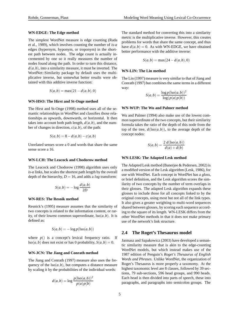
The models’ results on the WS-353 task are shown inFigure 3 and listed in Table 8. The COALS and LSAmodels all perform quite well on this task, with the high-est score of 65.7% achieved by COALS-SVD-800. How-ever, the WordNet and Roget’s models perform muchworse on the WS-353 set than they did on the previoustasks, with scores in the 34% to 39% range, although RO-GET is well ahead of the others. The WordNet modelstend to underestimate human judgments of the seman-tic similarity of associated or domain-related word-pairs,such as psychology–Freud, closet–clothes, and computer–software.
WS-400: Morphological and semantic word-pairclasses
The three word similarity tasks that we have just discussedwere limited mainly to noun-noun pairs of varying syn-onymy. However, we were also interested in the degreeto which human and model similarity judgments are af-fected by other factors, including syntactic role, morphol-ogy, and phonology.
Therefore, a survey was developed to determine thesemantic similarity of 400 pairs of words representinga range of lexical relationships (as shown in Table 9).Twenty different types of relationship were included, with20 pairs of words for each type. Some pairs were morpho-logically related (e.g., teacher-teach), some were mem-bers of the same taxonomic category (apple-pear), somewere synonyms (dog-hound), some shared only phono-logical similarity (catalog-cat), and others were dissimilarboth in meaning and in sound (steering-cotton).
The word pairs were divided into 10 lists with 40 wordson each list, 2 from each category of lexical relationship.The 10 lists were administered to 333 Carnegie Mellonundergraduates, such that each word pair was rated byan average of 33 participants. Participants were askedto rate the word pairs on a scale from 1 (very dissimilar)to 9 (very similar) and were encouraged to use the entirescale. The instructions included examples of highly simi-lar, moderately similar, and dissimilar pairs, and remindedparticipants that some words sound alike but neverthelesshave quite different meanings (e.g., ponder-pond). Ta-ble 9 shows the mean similarity ratings and frequency foreach type of word pair (Kucera & Francis, 1967).
The WS-400 words tend to be relatively common, witha GM frequency of 18.46 per million, just under twice thatof the Rubenstein and Goodenough (1965) words. Thescores of the models using all 400 of these pairs are givenin Figure 4 and Table 8. The outcome is similar to thatof the WS-353 task. COALS and LSA perform the best,
12
Rohde, Gonnerman, Plaut Modeling Word Meaning Using Lexical Co-Occurrence
0% 10% 20% 30% 40% 50% 60% 70% 80% 90% 100%
COALS-14KCOALS-SVD-800COALS-SVD-200HAL-14KHAL-400LSAWN-EDGEWN-HSOWN-LCHWN-RESWN-JCNWN-LINWN-WUPWN-LESKROGET
Figure 3: Performance of the models on the Finkelstein et al. (WS-353) task.
Table 9The 20 WS-400 word pair types for which human similarity ratings were obtained.
Type Example Description Mean Mean SimilarityFrequency Rating (std. dev.)
A. similarity–talented unrelated filler pair 61.8 1.54 (1.04)B. fasten–fast orthographically similar but unrelated foil 49.8 1.63 (0.99)C. fish–monkey distantly related coordinate nouns 23.2 3.08 (1.61)D. smoke–eat distantly related coordinate verbs 47.0 3.64 (1.72)E. lion–mane object and one of its parts 68.3 4.66 (1.81)F. cow–goat closely related coordinate nouns 39.1 5.19 (2.36)G. mailman–mail noun ending in -man and related noun or verb 40.2 5.34 (1.86)H. fly–drive closely related coordinate verbs 41.2 5.43 (1.75)I. entertain–sing superordinate-subordinate verb pair 64.3 5.48 (1.63)J. scientist–science noun or verb ending in -ist and related noun or verb 43.5 5.54 (1.74)K. stove–heat instrument and its associated action 45.4 5.91 (1.77)L. musician–play noun ending in -ian and related noun or verb 58.5 6.22 (1.73)M. weapon–knife superordinate-subordinate noun pair 47.6 6.30 (1.48)N. doctor–treat human agent and associated action 49.1 6.45 (1.65)O. famous–fame adjective and its related noun 50.2 6.73 (1.56)P. cry–weep synonymous verbs 48.9 6.88 (1.55)Q. rough–uneven synonymous adjectives 60.6 7.13 (1.66)R. farm–ranch synonymous nouns 74.6 7.37 (1.34)S. speak–spoken irregular noun or verb inflection 60.0 7.52 (1.55)T. monster–monsters regular noun or verb inflection 48.6 7.71 (1.42)
13
Rohde, Gonnerman, Plaut Modeling Word Meaning Using Lexical Co-Occurrence
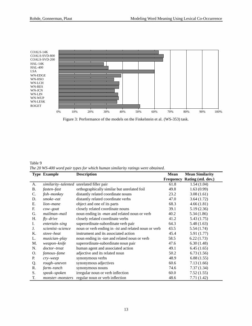
with COALS-SVD-800 scoring 68.4%, followed by RO-GET and then the WordNet models. WN-HSO performssomewhat better than the other WordNet methods on thistask. The HAL model performs very poorly on the WS-400 task.
This test is a bit unfair for the WordNet models becausethey were unable to handle 45 of the word pairs, mainlythose containing adjectives. ROGET was unable to han-dle 12 and the LSA model two. To verify that the inclu-sion of adjectives was not responsible for the relativelylow scores of the WordNet models, the WS-400-NV sub-task was constructed, involving 338 of the 400 pairs usingonly nouns and verbs. All of these pairs were recognizedby the models with the exception of ROGET and LSA,which were each unfamiliar with two pairs. This changeincreased the performance of the WordNet models by 8to 10 points, with the exception of WN-HSO and WN-LESK. Nevertheless, none of the WordNet models scoredover 50% on the WS-400-NV set.
Some of the WS-400 pairs are more difficult for thevector-based models because they induce human raters tomake use of a non-dominant word sense. In order to iden-tify these pairs, three judges were provided with the list ofpairs along with a list of the ten nearest neighbors (mostsimilar words) of each word, according to COALS. Thejudges indicated if the word senses they would use in com-paring the two words differ substantially from the sensessuggested by the nearest neighbors list. On 90 of the pairs,two of the three judges agreed that a non-dominant sensewas involved. The resulting 310 pairs form the WS-400-ND set. Once again, as we might expect, the performanceof the vector-based models increases significantly, whilethat of the WordNet models increases by just a few points,with no change for ROGET.
These results would seem to suggest that the vectorbased methods are substantially hindered by their lack ofword sense distinctions. While that is true to some extent,the overall performance of the COALS and LSA modelsremains quite high despite this limitation. If these meth-ods were substantially hindered by the interference of in-appropriate word senses, we should expect them to per-form very poorly on the 90 pairs relying on non-dominantsenses that were eliminated in forming the WS-400-NDset. If we test the models on just these 90 pairs, the HALscores do indeed drop to about -10%, but the COALSand LSA models remain quite strong. COALS-SVD-800achieves a score of 42.5%, with LSA scoring 41.3% andCOALS-14K scoring 37.0%. In contrast, the WordNetmodels all score between 10.3% (WN-WUP) and 32.8%(WN-HSO). The only model to outperform COALS andLSA is ROGET, scoring 56.0%. Therefore, even on wordpairs invoking a non-dominant sense, COALS and LSAcontinue to perform reasonably well.
A principal motivation for collecting the WS-400 rat-
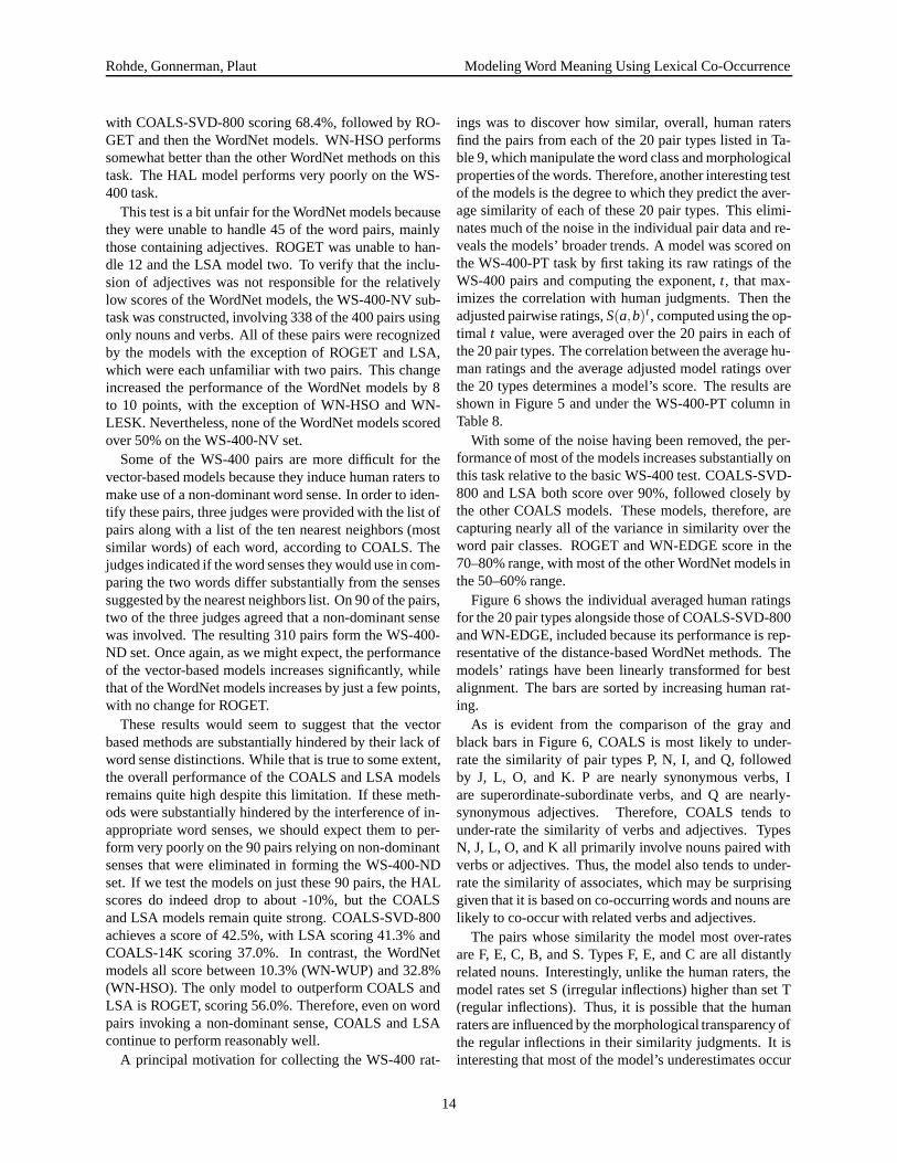
ings was to discover how similar, overall, human ratersfind the pairs from each of the 20 pair types listed in Ta-ble 9, which manipulate the word class and morphologicalproperties of the words. Therefore, another interesting testof the models is the degree to which they predict the aver-age similarity of each of these 20 pair types. This elimi-nates much of the noise in the individual pair data and re-veals the models’ broader trends. A model was scored onthe WS-400-PT task by first taking its raw ratings of theWS-400 pairs and computing the exponent, t, that max-imizes the correlation with human judgments. Then theadjusted pairwise ratings, S(a,b)t , computed using the op-timal t value, were averaged over the 20 pairs in each ofthe 20 pair types. The correlation between the average hu-man ratings and the average adjusted model ratings overthe 20 types determines a model’s score. The results areshown in Figure 5 and under the WS-400-PT column inTable 8.
With some of the noise having been removed, the per-formance of most of the models increases substantially onthis task relative to the basic WS-400 test. COALS-SVD-800 and LSA both score over 90%, followed closely bythe other COALS models. These models, therefore, arecapturing nearly all of the variance in similarity over theword pair classes. ROGET and WN-EDGE score in the70–80% range, with most of the other WordNet models inthe 50–60% range.
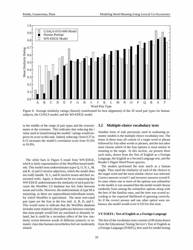
Figure 6 shows the individual averaged human ratingsfor the 20 pair types alongside those of COALS-SVD-800and WN-EDGE, included because its performance is rep-resentative of the distance-based WordNet methods. Themodels’ ratings have been linearly transformed for bestalignment. The bars are sorted by increasing human rat-ing.
As is evident from the comparison of the gray andblack bars in Figure 6, COALS is most likely to under-rate the similarity of pair types P, N, I, and Q, followedby J, L, O, and K. P are nearly synonymous verbs, Iare superordinate-subordinate verbs, and Q are nearly-synonymous adjectives. Therefore, COALS tends tounder-rate the similarity of verbs and adjectives. TypesN, J, L, O, and K all primarily involve nouns paired withverbs or adjectives. Thus, the model also tends to under-rate the similarity of associates, which may be surprisinggiven that it is based on co-occurring words and nouns arelikely to co-occur with related verbs and adjectives.
The pairs whose similarity the model most over-ratesare F, E, C, B, and S. Types F, E, and C are all distantlyrelated nouns. Interestingly, unlike the human raters, themodel rates set S (irregular inflections) higher than set T(regular inflections). Thus, it is possible that the humanraters are influenced by the morphological transparency ofthe regular inflections in their similarity judgments. It isinteresting that most of the model’s underestimates occur
14

Rohde, Gonnerman, Plaut Modeling Word Meaning Using Lexical Co-Occurrence
0% 10% 20% 30% 40% 50% 60% 70% 80% 90% 100%
COALS-14KCOALS-SVD-800COALS-SVD-200HAL-14KHAL-400LSAWN-EDGEWN-HSOWN-LCHWN-RESWN-JCNWN-LINWN-WUPWN-LESKROGET
Figure 4: Performance of the models across all word pairs on the WS-400 task.
0% 10% 20% 30% 40% 50% 60% 70% 80% 90% 100%
COALS-14KCOALS-SVD-800COALS-SVD-200HAL-14KHAL-400LSAWN-EDGEWN-HSOWN-LCHWN-RESWN-JCNWN-LINWN-WUPWN-LESKROGET
Figure 5: Performance of the models with the ratings averaged over each of the 20 word pair types on the WS-400task.
15
Rohde, Gonnerman, Plaut Modeling Word Meaning Using Lexical Co-Occurrence
A B C D E F G H I J K L M N O P Q R S TWord Pair Type
0.0
0.1
0.2
0.3
0.4
0.5
0.6
0.7
0.8
0.9
1.0M
ean
Sim
ilari
ty R
atin
g
COALS-SVD-800 ModelHuman RatingsWN-EDGE Model
Figure 6: Average similarity ratings (linearly transformed for best alignment) of the 20 word pair types for humansubjects, the COALS model, and the WS-EDGE model.
in the middle of the range of pair types and the overesti-mates at the extremes. This indicates that reducing the tvalue used in transforming the models’ ratings would im-prove its score in this task. Indeed, reducing t from 0.37 to0.15 increases the model’s correlation score from 91.6%to 93.9%.
The white bars in Figure 6 result from WN-EDGE,which is fairly representative of the WordNet-based meth-ods. This model most underestimates types Q, O, N, L, M,and K. Q and O involve adjectives, which the model doesnot really handle. N, L, and K involve nouns and their as-sociated verbs. Again, it should not be too surprising thatWN-EDGE underestimates the similarity of such pairs be-cause the WordNet 2.0 database has few links betweennouns and verbs. However, the underestimate of type M issurprising, as these are superordinate/subordinate nouns,for which WordNet is specialized. The most over-ratedpair types are the four at the low end: A, B, D, and C.This would seem to indicate that the WordNet databaseincludes some relatively short pathways between conceptsthat most people would feel are unrelated or distantly re-lated, but it could be a secondary effect of the low sim-ilarity scores between words of different syntactic or se-mantic class that humans nevertheless feel are moderatelyrelated.
3.2 Multiple-choice vocabulary tests
Another form of task previously used in evaluating se-mantic models is the multiple choice vocabulary test. Theitems in these tests all consist of a target word or phrasefollowed by four other words or phrases, and the test takermust choose which of the four options is most similar inmeaning to the target. In this section, we present threesuch tasks, drawn from the Test of English as a ForeignLanguage, the English as a Second Language test, and theReader’s Digest Word Power quizzes.
The models performed the tests much as a humanmight. They rated the similarity of each of the choices tothe target word and the most similar choice was selected.Correct answers scored 1 and incorrect answers scored 0.In cases where one or more of the options was unfamiliarto the model, it was assumed that the model would chooserandomly from among the unfamiliar options along withthe best of the familiar ones, and the item was scored ac-cording to the expected likelihood of guessing correctly.So if the correct answer and one other option were un-known, the model would score 0.333 for that item.
VT-TOEFL: Test of English as a Foreign Language
The first of the vocabulary tests consists of 80 items drawnfrom the Educational Testing Service’s Test of English asa Foreign Language (TOEFL), first used for model testing
16

Rohde, Gonnerman, Plaut Modeling Word Meaning Using Lexical Co-Occurrence
by Landauer and Dumais (1997). The items in this test allconsisted of single-word targets and options, such as con-cisely, prolific, or hue, with a fairly low GM frequencyof 6.94 per million. According to Landauer and Dumais(1997), a large sample of foreign college applicants tak-ing this or similar tests scored an average of 64.5% of theitems correct.
Table 8 shows the models’ results on the VT-TOEFLtask. The COALS models achieved the highest scores,with 88.8% for COALS-SVD-800, and 86.2% for the oth-ers. WN-LESK and ROGET also did well, with 79.7%and 74.6%, respectively, followed by WN-HSO at 67.8%.The HAL and LSA models scored in the mid 50–60%range and the other WordNet models scored in the low tomid 40’s. Landauer and Dumais (1997) reported a scoreof 64.4% for their model, higher than the 53.4% that wefound. The difference may be due to changes in the train-ing corpus, algorithm, or number of dimensions used.
The VT-TOEFL task is not quite fair to the Word-Net methods because it includes items involving adjec-tives and adverbs that are not well-represented in Word-Net. Therefore we also tested the VT-TOEFL-NV sub-set, consisting of just the 38 noun and verb items. In us-ing this subset, the performance of the vector-based mod-els declines slightly, although COALS-SVD-800 is stillthe best. As expected, the performance of the WordNetmodels, with the exception of WN-LESK, increases sig-nificantly. But they remain well behind ROGET and theCOALS models.
VT-ESL: English as a Second Language tests
The second vocabulary test consists of 50 items drawnfrom the English as a Second Language (ESL) test (Tur-ney, 2001). The ESL words tend to be shorter and higherin frequency (GM frequency 14.17 per million), but thetest relies on more subtle discriminations of meaning,such as the fact that passage is more similar to hallwaythan to entrance or that stem is more similar to stalk thanto trunk. In the actual ESL questions, the target wordswere placed in a sentence context, which often helps dis-ambiguate its meaning, but these contexts were not madeavailable to the models. Therefore, some items were dif-ficult or impossible, such as one in which the correct syn-onym for mass was lump, rather than service or worship.
The vector-based models did not perform as well onthe VT-ESL task as they did on VT-TOEFL. This may bebecause the ESL items often play on the distinction be-tween different senses of a word. The best performancewas achieved by ROGET followed by some of the Word-Net models and COALS-SVD-800. LSA was at 43.0%and the HAL models were at chance. Once again, a re-duced set of the 40 items using only nouns and verbs wasalso tested. This resulted in improved performance for the
WordNet models and a smaller improvement for ROGET,which again earned the highest score.
VT-RDWP: Reader’s Digest Word Power tests
The final vocabulary test consists of 300 items taken fromthe Reader’s Digest Word Power (RDWP) quizzes (Jar-masz & Szpakowicz, 2003). The GM frequency of thewords in these quizzes, 6.28 per million, is relatively lowand, unlike the other tests, the RDWP targets and op-tions are often multi-word phrases. The function wordswere removed from the phrases for our tests. Thesephrases were handled differently in the various models.The COALS and HAL models computed a vector for eachphrase by averaging the vectors of its words. For the LSAmodel, each phrase was treated as a text and the term-by-term similarity of the texts was computed. The WordNetand ROGET models do not have a natural way of dealingwith phrases. Therefore, the similarity between phraseswas taken to be that of the most similar pair of wordsspanning them.
The VT-RDWP task proved harder for the models thandid the VT-TOEFL and VT-ESL tasks. The best modelwas again ROGET, followed by WN-LESK and thenCOALS-SVD-800 and the other COALS models. Theother WordNet models and the HAL and LSA modelsall fared quite poorly. On the subset of 213 items usingonly nouns and verbs, VT-RDWP-NV, the performance ofmost of the WordNet models as well as the better COALSmodels improved. In this case, COALS-SVD-800 had thehighest score.
Overall Vocabulary Test Results
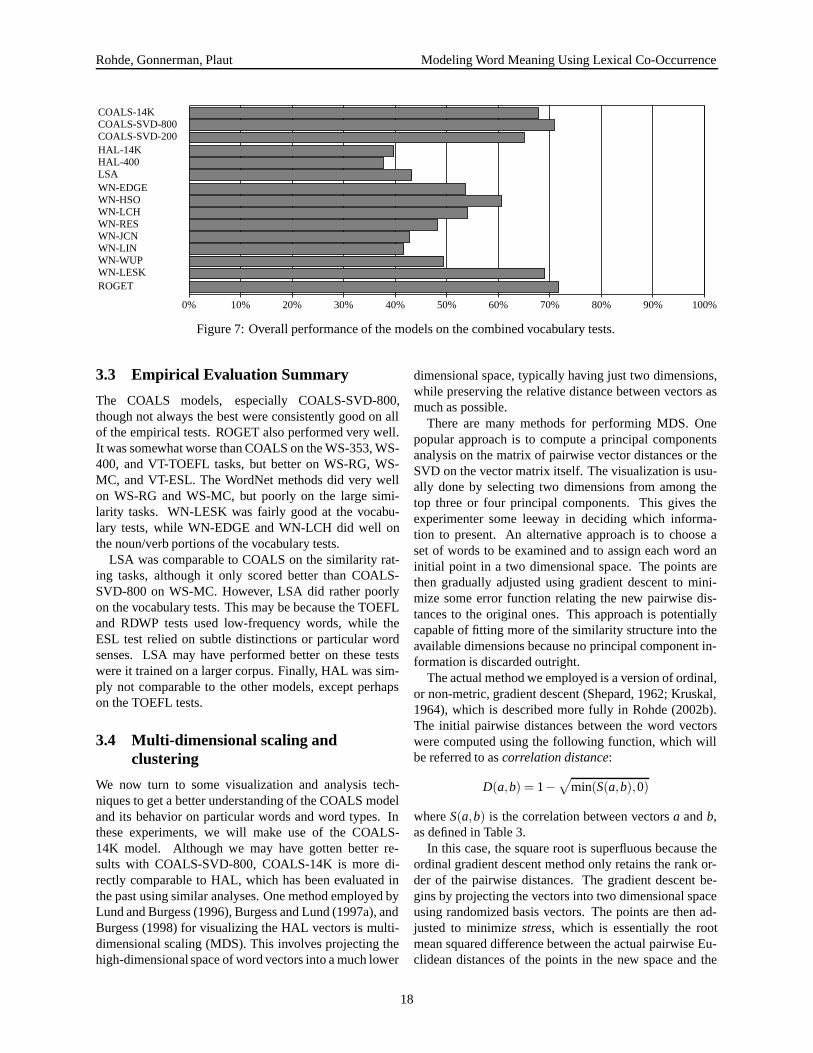
Figure 7 and Table 8 show the overall results on a com-bination of the 430 items in the three vocabulary tests.ROGET had the best score, followed closely by COALS-SVD-800 and WN-LESK. WN-HSO proved better thanthe other link-based WordNet methods, possibly becauseit makes use of a larger subset of the available links. TheWordNet models were the only ones sensitive to the pres-ence of adjectives and adverbs in the vocabulary tests.With the exception of WN-HSO and WN-LESK, theirperformance was 9% to 15% higher on the noun/verbitems.
The VT-ALL-NV column in Table 8 lists the overall re-sults on the 291 items using only nouns or verbs from thethree vocabulary tests. The performance of most of themodels on this subset is similar to their performance onthe full set of items. Most of the WordNet models im-prove, but the best of them—WN-EDGE, WN-LCH, andWN-LESK—remain somewhat worse than ROGET andCOALS-SVD-800.
17
Rohde, Gonnerman, Plaut Modeling Word Meaning Using Lexical Co-Occurrence
0% 10% 20% 30% 40% 50% 60% 70% 80% 90% 100%
COALS-14KCOALS-SVD-800COALS-SVD-200HAL-14KHAL-400LSAWN-EDGEWN-HSOWN-LCHWN-RESWN-JCNWN-LINWN-WUPWN-LESKROGET
Figure 7: Overall performance of the models on the combined vocabulary tests.
3.3 Empirical Evaluation Summary
The COALS models, especially COALS-SVD-800,though not always the best were consistently good on allof the empirical tests. ROGET also performed very well.It was somewhat worse than COALS on the WS-353, WS-400, and VT-TOEFL tasks, but better on WS-RG, WS-MC, and VT-ESL. The WordNet methods did very wellon WS-RG and WS-MC, but poorly on the large simi-larity tasks. WN-LESK was fairly good at the vocabu-lary tests, while WN-EDGE and WN-LCH did well onthe noun/verb portions of the vocabulary tests.
LSA was comparable to COALS on the similarity rat-ing tasks, although it only scored better than COALS-SVD-800 on WS-MC. However, LSA did rather poorlyon the vocabulary tests. This may be because the TOEFLand RDWP tests used low-frequency words, while theESL test relied on subtle distinctions or particular wordsenses. LSA may have performed better on these testswere it trained on a larger corpus. Finally, HAL was sim-ply not comparable to the other models, except perhapson the TOEFL tests.
3.4 Multi-dimensional scaling andclustering
We now turn to some visualization and analysis tech-niques to get a better understanding of the COALS modeland its behavior on particular words and word types. Inthese experiments, we will make use of the COALS-14K model. Although we may have gotten better re-sults with COALS-SVD-800, COALS-14K is more di-rectly comparable to HAL, which has been evaluated inthe past using similar analyses. One method employed byLund and Burgess (1996), Burgess and Lund (1997a), andBurgess (1998) for visualizing the HAL vectors is multi-dimensional scaling (MDS). This involves projecting thehigh-dimensional space of word vectors into a much lower
dimensional space, typically having just two dimensions,while preserving the relative distance between vectors asmuch as possible.
There are many methods for performing MDS. Onepopular approach is to compute a principal componentsanalysis on the matrix of pairwise vector distances or theSVD on the vector matrix itself. The visualization is usu-ally done by selecting two dimensions from among thetop three or four principal components. This gives theexperimenter some leeway in deciding which informa-tion to present. An alternative approach is to choose aset of words to be examined and to assign each word aninitial point in a two dimensional space. The points arethen gradually adjusted using gradient descent to mini-mize some error function relating the new pairwise dis-tances to the original ones. This approach is potentiallycapable of fitting more of the similarity structure into theavailable dimensions because no principal component in-formation is discarded outright.
The actual method we employed is a version of ordinal,or non-metric, gradient descent (Shepard, 1962; Kruskal,1964), which is described more fully in Rohde (2002b).The initial pairwise distances between the word vectorswere computed using the following function, which willbe referred to as correlation distance:
D(a,b) = 1−√
min(S(a,b),0)
where S(a,b) is the correlation between vectors a and b,as defined in Table 3.
In this case, the square root is superfluous because theordinal gradient descent method only retains the rank or-der of the pairwise distances. The gradient descent be-gins by projecting the vectors into two dimensional spaceusing randomized basis vectors. The points are then ad-justed to minimize stress, which is essentially the rootmean squared difference between the actual pairwise Eu-clidean distances of the points in the new space and the
18

Rohde, Gonnerman, Plaut Modeling Word Meaning Using Lexical Co-Occurrence
closest possible set of Euclidean distances that are con-strained to share the rank order of the pairwise correlationdistances of the original vectors. An automatic learningrate adjustment procedure is used to control the gradientdescent. Because this technique does not always find theglobally optimum possible arrangement, six trials wereperformed for each scaling problem and the solution withminimal stress was chosen. Typically, two or three of thetrials achieved similar minimal stress values.
Noun types
In this experiment, COALS vectors were obtained for 40nouns selected from three main classes: animals, bodyparts, and geographical locations. The MDS of thesewords is shown in Figure 8. Results for the HAL methodusing many of these same words are displayed in Fig-ure 2 of Lund and Burgess (1996), Figure 2 of Burgessand Lund (1997a), and Figure 2 of Burgess (1998). Vi-sual comparison with these figures should indicate that thecurrent method obtains a much tighter clustering of thesenoun categories.
Body parts are all clustered in the upper left and ani-mals in the lower left. It is likely that mouse separatesfrom the other animals due to its computer sense, oysterbecause it is primarily a food, and bull because of its vul-gar sense. Interestingly, the places are also separated intotwo or three clusters. The countries and continents are inthe upper right and the cities and states are below. It ap-pears that the North American cities have been separatedfrom the other places. One could speculate that Moscowhas grouped closer to the countries because it is a capitalcity and is therefore often referred to in much the sameterms as a country, as in, “. . . easing the way for Moscowto export more to Western Europe.”
An alternative way to visualize the similarity struc-ture of a set of items is hierarchical clustering (Johnson,1967). This general technique also has many variants. Inthe version used here, pairwise distances are again com-puted using the correlation distance function. Initially,each point forms its own cluster. The two closest clus-ters are merged and their centroid computed to form thenew location of the cluster (average-link clustering). Thisprocess repeats until only one cluster remains. Figure 9shows the hierarchical clustering of the 40 nouns. Eachvertical line represents a cluster. The length of a hori-zontal line represents the correlation distance between thecentroid of a cluster and the centroid of its parent cluster.Note that, according to the correlation distance function,two points are not necessarily equidistant from their cen-troid.
The primary division that the clustering algorithm findsis between the places and the other nouns. Within theplaces, there is a distinction between the cities and the
states, countries and continents (plus Moscow). Withinthe set of body parts there is little structure. Wrist andankle are the closest pair, but the other body parts do nothave much substructure, as indicated by the series of in-creasingly longer horizontal lines merging the words ontothe main cluster one by one. Within the animals there isa cluster of domestic and farm animals. But these do notgroup with the other animals. Turtle and oyster are quiteclose, perhaps because they are foods.
It is notable that the multidimensional scaling and clus-tering techniques do not entirely agree. Both involve aconsiderable reduction, and therefore possible loss, of in-formation. Turtle is close to cow and lion in the MDSplot, but that is not apparent in the clustering. On theother hand, the clustering distinguishes the (non-capital)cities from the other places whereas the MDS plot placesHawaii close to Tokyo. Although France appeared togroup with China and Russia in the MDS plot, it doesn’tin the hierarchical clustering. MDS has the potentialto map quite different points onto nearby locations andclustering has the potential to display apparent structurewhere there is none or fail to find structure when it istoo complex. Therefore, visualization techniques such asthese should not be overly relied upon as indicators ofprecise pairwise similarity, but they can prove very use-ful for understanding general patterns in complex, high-dimensional data.
An alternative technique for quantitatively evaluatingthe quality of a set of predefined clusters is to comparethe average distance between points in different clustersto the average distance between points that share a cluster.By computing these distances using correlation distancein the original space, rather than in a reduced dimension-ality space, we can avoid the possible biases introducedby the dimensionality reduction. And rather than com-paring average pairwise distances, we will actually usethe root mean square (r.m.s.) between- and within-clusterdistances, although this has little bearing on these results.An effective way to combine these distances into a clusterscore is to divide their difference by their sum. The result-ing ratio will fall in the [-1, 1] range, with random clus-terings having an expected score of 0. Because nearestneighbors in the COALS space typically have a correla-tion distance of about 0.25, the maximum possible clusterscore is roughly 0.6.
If we define the four clusters in the noun categoriza-tion task to be those indicated by the four different sym-bols used in Figure 8, the r.m.s. between cluster distanceis 0.91, while the r.m.s. within cluster distance is 0.55,resulting in a cluster score of 0.247. The fact that thisscore is positive indicates that the clusters are in somesense meaningful. However, the absolute magnitude ofthis score has little meaning and it is best understood rel-ative to other cluster scores. For example, if we instead
19
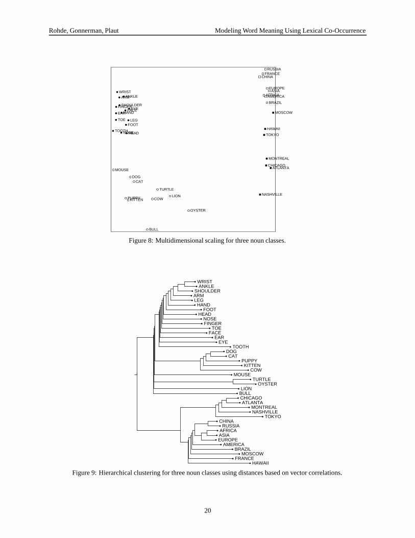
Rohde, Gonnerman, Plaut Modeling Word Meaning Using Lexical Co-Occurrence
HEAD
HANDFACE
DOG
AMERICA
CAT
EYE
EUROPE
FOOT
CHINAFRANCE
CHICAGO
ARM
FINGER
NOSE
LEG
RUSSIA
MOUSE
AFRICA
ATLANTA
EAR
SHOULDER
ASIA
COW
BULL
PUPPY LION
HAWAII
MONTREAL
TOKYO
TOE
MOSCOW
TOOTH
NASHVILLE
BRAZIL
WRIST
KITTEN
ANKLE
TURTLE
OYSTER
Figure 8: Multidimensional scaling for three noun classes.
WRISTANKLE
SHOULDERARMLEG
HANDFOOT
HEADNOSEFINGER
TOEFACE
EAREYE
TOOTHDOGCAT
PUPPYKITTEN
COWMOUSE
TURTLEOYSTER
LIONBULLCHICAGOATLANTA
MONTREALNASHVILLE
TOKYOCHINA
RUSSIAAFRICAASIAEUROPE
AMERICABRAZIL
MOSCOWFRANCE
HAWAII
Figure 9: Hierarchical clustering for three noun classes using distances based on vector correlations.
20

Rohde, Gonnerman, Plaut Modeling Word Meaning Using Lexical Co-Occurrence
define three clusters, with just one cluster containing allof the places, the cluster score falls to 0.222. The factthat placing small (cities and states) and large (countriesand continents) geographical areas in distinct clusters in-creases the cluster score provides further evidence that themodel is finding a substantive distinction between them.
Verb types
The next area we will look at are verb classes. Verbs are,arguably, more complex than nouns in that there are anumber of dimensions, both syntactic and semantic, onwhich they can vary. Verbs can be distinguished by tenseand aspect, argument structure, and on other syntactic lev-els, in addition to semantic differences. But there is oftena noticeable correlation between verb meaning and argu-ment structure (Levin, 1993). For example, verbs thatinvolve giving or sending generally take a dative object,while thought verbs (think, believe, know) can usuallytake a sentential complement. If the model assigns thoseverbs similar representations, is it due to their syntactic orsemantic similarity? Certainly, it will be some combina-tion of the two and one interesting question is the degreeto which COALS is sensitive to syntax versus semantics.
We begin by looking at eight common verbs selectedfrom each of three semantic classes: violent action verbs,verbs of sensation, and verbs of communication. Asshown in Figure 10, the verbs of each class do group to-gether in the multidimensional scaling, but the clusters arenot as tight as for the noun classes. Action verbs are in thelower right of the plot, communication in the lower leftand sensation in the upper half. The points are not evenlydistributed in the space because detected and cut are out-liers that fall at the extremes of their classes. According tothis plot, the model does not seem to be particularly sen-sitive to argument structure, as there is not a clear distinc-tion between the communication verbs that are frequentlyditransitive (told, asked) and those that usually take a sin-gle object (explained, questioned) or no object (shouted).However, the model does seem to be reasonably sensitiveto the semantic distinctions between the verbs. The over-all cluster score for this set of verbs is 0.078, which isconsiderably lower than the score on the noun clusteringtask.
To further investigate the model’s bias towards seman-tic over syntactic distinctions, the next MDS experimentinvolved eight verb roots in each of four forms: presenttense, past tense, progressive (-ing), and past participle.As shown in Figure 11, the verbs are tightly clustered onthe basis of verb root, rather than on syntactic form. Whendivided according to root, the cluster score is a very strong0.375. This suggests that the model may be purely drivenby semantics, with no consistent contribution from syn-tax.
However, an additional experiment, shown in Fig-ure 12, leads to a seemingly contradictory outcome. Inthis case, we have selected 12 verb roots, including theeight from Figure 11, and performed a multidimensionalscaling using just their past tense and past participleforms, which are all unambiguous. Although the cluster-ing is not particularly tight, with a score of 0.078, there isa clear and consistent effect of syntactic form. All of thepast tenses align on the bottom and the past participles ontop.
The MDS analyses in Figures 11 and 12 would appearto be contradictory. In the first case, verb root dominates,while in the second case verb type appears to be the dom-inant factor. Further analysis using the cluster score in-dicates that COALS itself is behaving in a relatively con-sistent manner. On the first task, shown in Figure 11, thescore when clustering on the basis of verb root was 0.375.However, if we instead categorize the verbs on the basis ofsyntactic form, the clustering score is 0.061. While sub-stantially lower, this score is still highly significant and themean correlations within and across the clusters are sta-tistically different (F(1,494)=17.32, p < 0.0001). There-fore, although the model’s vectors primarily reflect prop-erties of verb roots, there is also a consistent syntactic, orverb form, component. The same is true for the verb pairsshown in Figure 12. The clustering score computed onthe basis of syntactic form was, in this case, 0.078, whichis only a bit stronger than the 0.061 on the previous ex-periment. But if the clustering score is computed on thebasis of verb root, it is 0.240. Therefore, in both cases themodel’s representations of the verbs primarily reflectedverb root, while syntactic form plays a noticeable, thoughweaker, role.
How can two MDS analyses lead to such apparentlycontradictory results, such as those in Figures 11 and 12?The answer lies in the potentially misleading effect of in-formation loss resulting from MDS. Vectors in a high-dimensional space can have a complex similarity struc-ture. The vector representing some concept might, forexample, be composed of features reflecting a variety ofproperties, such as its size, its shape, its appearance, itsuse, where it comes from, whether it is dangerous, and soforth. Thus, a stuffed bear and a toy car might be similarbecause they are both small toys that children play with.And a toy car and a real car are similar at different levels:in appearance and, metaphorically, in use. But a stuffedbear and a real car don’t have all that much in common.When a set of vectors that differ on a variety of levels arerearranged in a two-dimensional space, there are simplynot enough degrees of freedom to capture the full com-plexity the similarity structure. The best low-dimensionalrepresentation can be obtained by allowing the most con-sistently relevant components to dominate.
In Figure 11, the semantic distinctions between verb
21
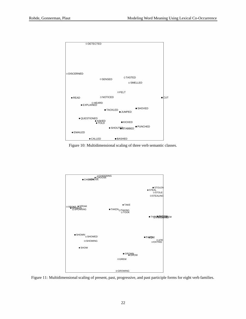
Rohde, Gonnerman, Plaut Modeling Word Meaning Using Lexical Co-Occurrence
READ
CALLED
TOLD
HEARD
ASKED
CUT
FELT
NOTICED
EXPLAINED
KICKED
JUMPED
DETECTED
EMAILED
QUESTIONED
SHOUTED
TASTED
PUNCHED
SHOVED
STABBED
SMELLEDSENSED
BASHED
TACKLED
DISCERNED
Figure 10: Multidimensional scaling of three verb semantic classes.
TAKE
SHOW
TOOKTAKINGTAKEN
SPEAK
EAT
CHOOSE
SPEAKING
GROW
GROWING
THROW
SHOWN
SHOWING
SHOWED
EATING
CHOSEN
SPOKE
CHOSE
GROWN
GREW
SPOKEN
THROWNTHROWING
STEAL
ATE
THREW
STOLEN
STEALING
CHOOSING
STOLE
EATEN
Figure 11: Multidimensional scaling of present, past, progressive, and past participle forms for eight verb families.
22

Rohde, Gonnerman, Plaut Modeling Word Meaning Using Lexical Co-Occurrence
WROTE
TOOK
KNOWN
TAKEN
KNEW
WRITTEN SHOWN
SHOWED
CHOSEN
SPOKE
CHOSE
DRIVEN
GROWN
DREW
GREW
SPOKEN
THROWN
DRAWN
ATETHREW
DROVE
STOLEN
STOLE
EATEN
Figure 12: Multidimensional scaling of unambiguous past tense and past participle verb forms.
roots dominate and mask the weaker effects of syntacticsimilarity. With four different verb forms, there wouldbe no way, in this constrained space, to place verb formsfrom the same root close together and also place verbswith the same syntactic form closer to one another than tothe other verbs. On the other hand, in Figure 12, wherethere is a single syntactic contrast, the consistent effectof this component across all pairs balances the semanticcomponents and draws the past tenses to one side and thepast participles to the other. In this case, the stronger se-mantic similarity structure is not as apparent, though itis not completely lost. Although multidimensional scal-ing and hierarchical clustering, which suffers from a sim-ilar problem, are useful tools for visualization of complexdata, they can be misleading and are best used in conjunc-tion with other methods, such as the clustering score.
Noun/verb associates
This final study asks the question, “How much teach isin a teacher?” That is, how similar are the COALS rep-resentations for an agentive noun and its associated ac-tion, relative to the similarity between different agentivenouns. Eight word pairs were selected, each including anoun denoting a common human occupation or role and averb denoting a typical action in which that person mightengage. The MDS results for this data set are shown inFigure 13. The nouns occupy the upper right of the spaceand the verbs the lower left. However, the noun vs. verbclustering is not particularly tight, with a score of 0.065.
It is also apparent that nouns and their associated verbsare correlated in their position along the line separatingnouns from verbs, with driver/drive in the upper left andpriest/pray and bride/marry (as well as priest/marry) inthe lower right. If each of the associated nouns and verbsare paired, the clustering score increases to 0.134. The av-erage correlation distance between nouns and their associ-ated verbs is 0.64, compared to a distance of 0.77 betweennouns and 0.90 between nouns and non-associated verbs.Therefore, according to the model, semantic domain has astronger effect than word class, so teacher includes some-what more teach than it does –er.
3.5 Nearest neighbors
Another way to gain a visceral sense for what the COALSvectors are encoding is to look at the nearest neighbors,in semantic space, of various words. Table 10 shows the10 nearest neighbors, out of the 100,000 most commonwords, for some representative nouns. As a point of com-parison, similar lists based on HAL can be found for someof these words in Table 2 of Lund and Burgess (1996).
For unambiguous nouns with many near synonyms orsubtypes, such as gun, the model is quite effective at find-ing those synonyms. Singular and plural noun forms tendto have very similar representations. For a word like card-board, the model mainly identifies correlates, meaningother types of material. For Leningrad, it finds placesin Russia, or words associated with it, rather than othercities of the world. But the similarity of these neighbors
23

Rohde, Gonnerman, Plaut Modeling Word Meaning Using Lexical Co-Occurrence
DRIVE
LEARN
DOCTOR
CLEAN
DRIVER
STUDENT
TEACH
TEACHER
TREAT PRAY
PRIEST
MARRY
SWIMBRIDE
JANITORSWIMMER
Figure 13: Multidimensional scaling for nouns and their associated verbs.
Table 10The 10 nearest neighbors and their percent correlation similarities for a set of nouns, under the COALS-14K model.
gun point mind monopoly cardboard lipstick leningrad feet1) 46.4 handgun 32.4 points 33.5 minds 39.9 monopolies 47.4 plastic 42.9 shimmery 24.0 moscow 59.5 inches2) 41.1 firearms 29.2 argument 24.9 consciousness 27.8 monopolistic 37.2 foam 40.8 eyeliner 22.7 sevastopol 57.7 foot3) 41.0 firearm 25.4 question 23.2 thoughts 26.5 corporations 36.7 plywood 38.8 clinique 22.7 petersburg 52.0 metres4) 35.3 handguns 22.3 arguments 22.4 senses 25.0 government 35.6 paper 38.4 mascara 20.7 novosibirsk 45.7 legs5) 35.0 guns 21.5 idea 22.2 subconscious 23.2 ownership 34.8 corrugated 37.2 revlon 20.3 russia 45.4 centimeters6) 32.7 pistol 20.1 assertion 20.8 thinking 22.2 property 32.3 boxes 35.4 lipsticks 19.6 oblast 44.4 meters7) 26.3 weapon 19.5 premise 20.6 perception 22.2 capitalism 31.3 wooden 35.3 gloss 19.5 minsk 40.2 inch8) 24.4 rifles 19.3 moot 20.4 emotions 21.8 capitalist 31.0 glass 34.1 shimmer 19.2 stalingrad 38.4 shoulders9) 24.2 shotgun 18.9 distinction 20.1 brain 21.6 authority 30.7 fabric 33.6 blush 19.1 ussr 37.8 knees
10) 23.6 weapons 18.7 statement 19.9 psyche 21.3 subsidies 30.5 aluminum 33.5 nars 19.0 soviet 36.9 toes
Table 11The 10 nearest neighbors for a set of verbs, according to the COALS-14K model.
need buy play change send understand explain create1) 50.4 want 53.5 buying 63.5 playing 56.9 changing 55.0 sending 56.3 comprehend 53.0 understand 58.2 creating2) 50.2 needed 52.5 sell 55.5 played 55.3 changes 42.0 email 53.0 explain 46.3 describe 50.6 creates3) 42.1 needing 49.1 bought 47.6 plays 48.9 changed 40.2 e-mail 49.5 understood 40.0 explaining 45.1 develop4) 41.2 needs 41.8 purchase 37.2 players 32.2 adjust 39.8 unsubscribe 44.8 realize 39.8 comprehend 43.3 created5) 41.1 can 40.3 purchased 35.4 player 30.2 affect 37.3 mail 40.9 grasp 39.7 explained 42.6 generate6) 39.5 able 39.7 selling 33.8 game 29.5 modify 35.7 please 39.1 know 39.0 prove 37.8 build7) 36.3 try 38.2 sells 32.3 games 28.3 different 33.3 subscribe 38.8 believe 38.2 clarify 36.4 maintain8) 35.4 should 36.3 buys 29.0 listen 27.1 alter 33.1 receive 38.5 recognize 37.1 argue 36.4 produce9) 35.3 do 34.0 sale 26.8 playable 25.6 shift 32.7 submit 38.0 misunderstand 37.0 refute 35.4 integrate
10) 34.7 necessary 31.5 cheap 25.0 beat 25.1 altering 31.5 address 37.9 understands 35.9 tell 35.2 implement
Table 12The 10 nearest neighbors for a set of adjectives, according to the COALS-14K model.
high frightened red correct similar fast evil christian1) 57.5 low 45.6 scared 53.7 blue 59.0 incorrect 44.9 similiar 43.1 faster 24.3 sinful 48.5 catholic2) 51.9 higher 37.2 terrified 47.8 yellow 37.7 accurate 43.2 different 41.2 slow 23.4 wicked 48.1 protestant3) 43.4 lower 33.7 confused 45.1 purple 37.5 proper 40.8 same 37.8 slower 23.2 vile 47.9 christians4) 43.2 highest 33.3 frustrated 44.9 green 36.3 wrong 40.6 such 28.2 rapidly 22.5 demons 47.2 orthodox5) 35.9 lowest 32.6 worried 43.2 white 34.1 precise 37.7 specific 27.3 quicker 22.3 satan 47.1 religious6) 31.5 increases 32.4 embarrassed 42.8 black 32.9 exact 35.6 identical 26.8 quick 22.3 god 46.4 christianity7) 30.7 increase 32.3 angry 36.8 colored 30.7 erroneous 34.6 these 25.9 speeds 22.3 sinister 43.8 fundamentalist8) 29.2 increasing 31.6 afraid 35.6 orange 30.6 valid 34.4 unusual 25.8 quickly 22.0 immoral 43.5 jewish9) 28.7 increased 30.4 upset 33.5 grey 30.6 inaccurate 34.1 certain 25.5 speed 21.5 hateful 43.2 evangelical
10) 28.3 lowering 30.3 annoyed 32.4 reddish 29.8 acceptable 32.7 various 24.3 easy 21.3 sadistic 41.2 mormon
24

Rohde, Gonnerman, Plaut Modeling Word Meaning Using Lexical Co-Occurrence
Table 13The 10 nearest neighbors for a set of closed class words, according to the COALS-14K model.
he could where after three although into ?1) 81.1 she 75.3 can 29.8 outside 49.6 before 79.0 two 56.2 though 42.9 onto 56.7 <EMO>2) 51.6 he’d 60.2 would 28.3 somewhere 46.1 during 74.9 four 53.1 however 37.1 back 56.2 ...3) 49.6 they 58.0 can’t 27.9 nearby 41.7 later 71.7 five 52.8 but 36.7 down 53.9 lol4) 48.5 him 56.6 might 26.7 in 41.0 last 65.6 six 35.6 quite 35.4 inside 49.1 eh5) 48.0 who 56.5 couldn’t 26.7 near 38.3 ago 64.9 eight 34.6 that 34.8 slowly 48.6 huh6) 47.8 mulder 56.3 able 25.6 what 37.3 ended 60.9 seven 34.6 because 32.9 out 47.3 btw7) 47.8 she’d 50.7 will 24.5 how 37.0 until 59.6 several 33.9 certainly 31.9 away 47.0 yeah8) 47.3 someone 50.6 cannot 24.1 anywhere 36.7 afterwards 56.2 couple 32.3 seem 31.7 through 46.9 !9) 46.7 it 49.1 didn’t 23.4 there 36.2 since 54.8 few 31.6 also 31.1 around 45.2 hey
10) 46.6 nobody 48.4 you 23.2 secluded 35.7 started 48.8 nine 31.3 even 30.5 then 43.9 anyway
Table 14The 3 nearest neighbors for a set of misspelled words, according to the COALS-14K model.
paly carribean thanx dont thier refering definatly wierd1) 24.5 play 51.7 caribbean 74.9 thanks 78.6 don’t 59.1 their 38.5 referring 30.9 definitely 52.0 weird2) 18.8 playing 29.8 bahamas 49.9 tia (thanks in advance) 57.8 didn’t 36.7 own 22.5 talking 20.6 probably 36.7 strange3) 17.0 played 27.5 mediterranean 47.5 cheers 53.0 wouldn’t 35.0 our 22.3 refers 18.6 really 35.1 odd
is relatively weak. The nearest neighbors for lipstick aresomething of a mixed bag, with some correlates (eyeliner,mascara, gloss, blush), some companies that manufactureit (Clinique, Revlon, NARS), and some properties associ-ated with it (shimmery, shimmer).
In the case where one word sense is much more fre-quent than the others, the weaker senses will be over-whelmed. Consider the words point and mind. Point couldmean the sharp end of a pin, or it could mean a propo-sition. As seen in Table 10, the latter definition clearlydominates in our corpus. Likewise, mind could either bea noun or a verb (“Do you mind?”), but the noun senseappears to be dominant. Some words, on the other hand,have two roughly balanced senses, so the vector represent-ing the word will be close to the average of the vectors thatwould reflect the distinct senses. Is this a serious problemfor the model?
Consider generating two random vectors, x and y, in a1000-dimensional space and averaging them to produce z.Vectors x and y will be uncorrelated, but they each willhave a correlation with z of about 70%, which is quitestrong, stronger than the typical similarity between a pairof close synonyms. Therefore, if a word has two evenlybalanced senses, the vector average of those two mean-ings won’t be nonsense, but will remain highly correlatedwith each of the two senses, and thus with synonyms ofthose senses (Kawamoto, 1993; Hinton & Shallice, 1991).The word feet is a good illustration of this. Its two mainmeanings, the things you walk on and a unit of measure,are roughly evenly balanced in frequency and the nearestneighbors to feet, according to the model, reflect one orthe other of the two senses. Five of the ten neighbors areother units of measure, four are other body parts, and footis ambiguous.
Eight verbs and their nearest neighbors are listed in Ta-ble 11. The verb neighbors seem to contain fewer asso-
ciates and more synonyms or near synonyms, althoughsale and cheap are neighbors of buy, and different is aneighbor of change. Other forms of the same verb arealso generally high on the list. Obviously, the verb sendis biased in our corpus towards an email or newsgroupcontext. It isn’t clear if email is so high on its list be-cause the noun form of email is associated with sendingor because the verb form is somewhat synonymous. It isinteresting that game and games appear as neighbors ofplay. One might view these as associates; that is, wordsthat frequently appear together but are unrelated in mean-ing. However, they are not pure associates as they do seemto share some aspect of meaning—we might call it theirplayfulness. Overall, the verbs are more similar to theirnearest neighbors than the nouns are to theirs.
Table 12 displays the nearest neighbors for some adjec-tives. In this case, the neighbors are mainly a mixtureof synonyms, antonyms, and comparative forms (high,higher, highest). The color words are all deemed highlysimilar to one another. The word evil is ambiguous be-tween the adjective and noun forms, and appears to havesome associates as neighbors, such as demons and satan,although all of its neighbors are relatively weak.
Table 13 shows the nearest neighbors for some closedclass words. Many of the nearest neighbors for the func-tion words are of the same class as the target word, be it apronoun, modal, preposition, conjunction, or punctuation.But there do appear to be some associated words on thelist. He and she have a very high correlation similarity.Who is probably merely associated with he and Mulderis hard to explain, except that it and Scully, both charac-ters in the popular X-Files television show, happen to havebeen very frequent in our corpus. The nearest neighborsof after are not all prepositions, but they are all tempo-ral words. Interestingly, three was found to be similar notonly to other numbers but to the quantifiers several, cou-
25

Rohde, Gonnerman, Plaut Modeling Word Meaning Using Lexical Co-Occurrence
ple, and few. Presumably one is not as similar to threeas the other digits are because it is less often used as aquantifier and more often to mean someone. The near-est neighbors of the question mark tend to be other sym-bols and interjections that newsgroup writers use to end orbridge their sentences, such as emoticons (<EMO>) andthe abbreviations lol (laughing out loud) and btw (by theway).
It seems evident, on the basis of these nearest neigh-bor lists, that the COALS method produces quite reason-able responses on the whole. The nearest neighbors to aword are usually strongly semantically related, either syn-onyms, antonyms, coordinates, subordinates, or superor-dinates. But there is still some tendency for pure asso-ciates, such as could–you or buy–cheap, to be assignedsimilar representations. It may be inevitable that a modelbased on word co-occurrence will reflect pure associationto some degree, but this tendency is minimized in COALSby the use of a narrow neighborhood window and correla-tion normalization.
In one final example, we chose eight common mis-spellings that were missed by our automatic spellingcorrection procedure and found their nearest neighbors,shown in Table 14. Although COALS makes no use oforthography and doesn’t weight its nearest neighbors byfrequency, the semantic nearest neighbor for each of thesemisspellings is the correct spelling of the word. There-fore, it is likely that COALS could be used in conjunc-tion with some simple orthographic matching proceduresto create an effective spelling correction system for com-mon mistakes. It remains to be seen how well it wouldwork on unique or infrequent mistakes for which little co-occurrence data is available.
4 Variations on the COALS method
In this section, we explore the components of the COALSmodel that distinguish it from other vector-based modelsand contribute to its success. In particular, we examinealternative matrix normalization methods, the differencesbetween HAL and COALS, the effects of vector dimen-sionality on the performance of COALS, COALS-SVD,and COALS-SVDB, and the interaction between corpussize and the co-occurrence window size.
4.1 Vector normalization methods
HAL, LSA, and COALS all involve constructing a co-occurrence matrix and normalizing the cells of that matrixto accentuate the useful information it contains. Somepossible normalization functions were given in Table 4.HAL normalizes the length of each row vector, and thusthe sum of the squared components, to 1. A similar form
of row normalization scales the sum of the components to1. Neither of these methods has any effect on the correla-tion or cosine similarity measures, except when averagingvectors to produce representations of phrases on the VT-RDWP task. Row normalizations do nothing to reduce theinfluence of columns representing high frequency wordsor large documents. An alternative method that does dothis is column normalization, which scales each columnto a sum of 1.
The entropy normalization often used with LSA is amodified form of row normalization. It replaces each en-try with its log, which reduces but does not eliminate theinfluence of high frequency columns. Each row is thendivided by its entropy, so that rows without much varia-tion within them are discounted. This second step againhas no bearing if the row-wise correlation or cosine is tobe computed immediately, but it does affect a subsequentSVD.
The normalization method used in COALS initially re-places each cell in the matrix with the temporal correlationof the row and column items. This is relatively insensitiveto the overall frequency of both the row and column itemsand is therefore something like a simultaneous row andcolumn normalization. Negative values are then discardedand the positive values are square rooted to reduce the in-fluence of large correlations. Along with improving theperformance, this step has the added benefit of decreas-ing the density of the resulting matrix. Although they arenot very sparse, COALS matrices usually have a densityof about 15–20%, roughly half that of matrices producedwith the other normalization procedures, making the com-putation of the SVD more efficient.
Table 15 shows the effects of these various normaliza-tion procedures when used in place of square root cor-relation on the COALS and COALS-SVD models. Withthe exception of the normalization procedure, the modelsin the top half of the table are all identical to COALS-14K and those in the bottom half are identical to COALS-SVD-800. Using no normalization (-NONE) and usingrow normalization (-ROW) results in relatively poor per-formance. Without the SVD, they are equivalent exceptthat row normalization gives a slight improvement on themulti-word RDWP phrases. Because the correlation sim-ilarity function ignores the row magnitude, column nor-malization (-COL) works nearly as well as correlation onthe COALS model. But if used in conjunction with theSVD, column normalization by itself is ineffective. Theopposite is true for entropy normalization (-ENTR). It re-sults in no improvement without the SVD, but with theSVD it is quite effective.
The -COR variants are similar to the COALS models inthat they compute the correlation and discard the negativevalues, but they do not take the square root of the pos-itive correlations. There is little difference between this
26

Rohde, Gonnerman, Plaut Modeling Word Meaning Using Lexical Co-Occurrence
Table 15Performance of the COALS and COALS-SVD models using various normalization procedures.
Model WS-
RG
WS-
RG
-ND
WS-
MC
WS-
MC
-ND
WS-
353
WS-
400
WS-
400-
NV
WS-
400-
ND
WS-
400-
PT
VT-
TO
EF
L
VT-
TO
EF
L-N
V
VT-
ESL
VT-
ESL
-NV
VT-
RD
WP
VT-
RD
WP
-NV
VT-
AL
L
VT-
AL
L-N
V
Ove
rall
COALS-NONE 45.9 54.1 50.5 63.6 37.3 42.6 44.2 52.6 82.6 66.2 65.8 32.0 37.5 46.8 48.1 48.7 49.0 50.7COALS-ROW 45.9 54.1 50.5 63.6 37.3 42.6 44.2 52.6 82.6 66.2 65.8 32.0 37.5 50.8 52.8 51.5 52.4 51.4COALS-COL 64.6 75.0 63.6 78.2 61.4 64.0 63.2 70.7 92.4 78.8 79.0 52.0 57.5 57.5 58.0 60.6 60.6 67.1COALS-ENTR 46.1 51.3 48.9 67.1 35.7 38.4 37.7 45.2 77.5 66.2 65.8 40.0 45.0 53.8 51.9 54.3 52.8 50.5COALS-COR 67.3 76.7 67.8 80.7 59.3 62.8 63.1 71.0 90.8 83.8 81.6 54.0 55.0 61.2 62.2 64.3 63.8 68.3COALS-14K 68.2 79.1 67.1 85.2 62.6 62.4 60.9 71.2 88.0 86.2 81.6 52.0 52.5 65.5 67.4 67.8 67.2 69.2COALS-SVD-NONE 60.6 67.1 82.8 85.4 43.1 47.8 48.9 58.3 81.6 75.0 65.8 42.0 42.5 45.8 47.2 51.0 49.0 58.3COALS-SVD-ROW 60.3 69.1 61.2 75.0 52.3 56.4 57.1 64.5 90.0 70.0 60.5 46.0 50.0 50.8 50.0 53.8 51.4 60.5COALS-SVD-COL 51.1 58.2 49.8 66.6 48.0 54.0 52.2 64.5 91.4 72.5 68.4 36.0 37.5 45.2 45.3 49.0 47.2 55.9COALS-SVD-ENTR 67.1 76.6 73.3 83.3 66.1 68.1 67.3 72.6 88.4 86.2 84.2 66.0 65.0 61.5 60.3 66.4 64.1 71.5COALS-SVD-COR 49.6 55.5 37.1 45.9 47.8 52.1 51.8 64.2 87.5 61.2 60.5 40.0 42.5 47.5 45.8 49.0 47.2 53.2COALS-SVD-800 67.3 77.9 72.7 82.5 65.7 68.4 67.5 74.2 91.6 88.8 86.8 68.0 67.5 66.8 69.2 70.8 71.3 73.4
and the COALS procedure without the SVD. But with theSVD, taking the square roots of the correlations is muchmore effective. Both with and without the use of the SVDfor dimensionality reduction, the COALS normalizationprocedure results in the best overall performance on ourtasks.
4.2 Differences between the HAL andCOALS methods
In this section we take a closer look at the differences be-tween the HAL and COALS procedures and the effectsthese differences have on performance. Table 16 showsthe major performance measures for 13 different mod-els, ranging from the HAL procedure in model A to theCOALS procedure in model M.
All of these models use vectors with 14,000 compo-nents. The models with Distinct L/R checked make adistinction between neighboring words that occur to theleft and right of the target word when counting the co-occurrences. In these models, the 14,000 columns arechosen on the basis of highest variance. The other modelsdo not distinguish between left and right neighbors andselect the top columns on the basis of overall frequency.Window Size is the radius of the window around the targetword within which neighbors are counted. Window Shapeindicates whether the window is ramped, with a higherweighting for closer neighbors, or flat. Closed Class in-dicates whether closed class columns are included amongthe 14,000. Vector Norm. is the procedure used to nor-malize the matrix. Length is the vector length normaliza-tion used in HAL, while correl. is the square root positivecorrelation used in COALS. Finally, the Distance Func. is
the function used to compute vector similarity. Euclid. isthe inverse squared Euclidean distance and correl. is thecorrelation distance defined in Table 3.
The typical HAL model (A) has distinct left- and right-neighbor columns, a size 10 window, uses closed classcolumns, length normalization, and some form of Eu-clidean distance or similarity. In contrast, COALS doesnot have distinct left- and right-neighbor columns, usesa size 4 window, ignores closed class columns, and usescorrelation normalization and similarity functions. Wewill explore the importance of each of these differences.
Simply switching to a size 4 window under the HALmethod (B) is counter-productive. Not enough informa-tion is being separated from the noise in the co-occurrencedata for this difference to matter. A major problem withthe HAL length normalization procedure is that the vec-tors are dominated by high-frequency columns. Thus,eliminating the closed class columns (C), which are highfrequency but carry relatively little semantic information,results in a significant improvement in the model. ModelD is identical to B except that the correlation distancefunction is used, which results in no change in perfor-mance. Simply using correlation similarity without theright normalization is not helpful.
Model E is like B but uses correlation normalization,resulting in a significant improvement. Adding the cor-relation similarity measure on top of this (F) now leadsto further improvement. Ignoring closed class columnsas well (H) is better still. In this case, using a size 10window (G) is now somewhat less effective than the size4 window. Model I is similar to F but it does not makethe distinction between left and right neighbors. This im-proves the overall performance by several points. Now,
27
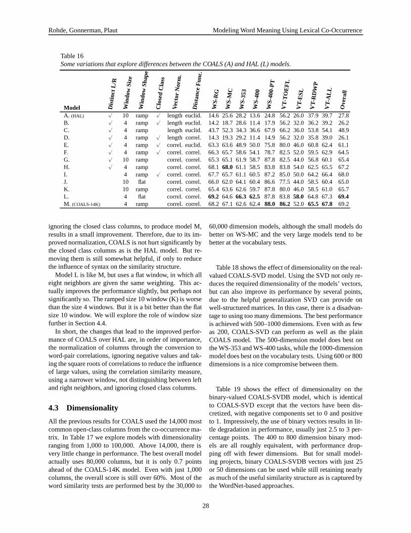
Rohde, Gonnerman, Plaut Modeling Word Meaning Using Lexical Co-Occurrence
Table 16Some variations that explore differences between the COALS (A) and HAL (L) models.
Model Dis
tinc
t L/R
Win
dow
Size
Win
dow
Shap
e
Clo
sed
Cla
ss
Vec
tor
Nor
m.
Dis
tanc
eF
unc.
WS-
RG
WS-
MC
WS-
353
WS-
400
WS-
400-
PT
VT-
TO
EF
L
VT-
ESL
VT-
RD
WP
VT-
AL
L
Ove
rall
A. (HAL)√
10 ramp√
length euclid. 14.6 25.6 28.2 13.6 24.8 56.2 26.0 37.9 39.7 27.8B.
√4 ramp
√length euclid. 14.2 18.7 28.6 11.4 17.9 56.2 32.0 36.2 39.2 26.2
C.√
4 ramp length euclid. 43.7 52.3 34.3 36.6 67.9 66.2 36.0 53.8 54.1 48.9D.
√4 ramp
√length correl. 14.3 19.3 29.2 11.4 14.9 56.2 32.0 35.8 39.0 26.1
E.√
4 ramp√
correl. euclid. 63.3 63.6 48.9 50.0 75.8 80.0 46.0 60.8 62.4 61.1F.
√4 ramp
√correl. correl. 66.3 65.7 58.6 54.1 78.7 82.5 52.0 59.5 62.9 64.5
G.√
10 ramp correl. correl. 65.3 65.1 61.9 58.7 87.8 82.5 44.0 56.8 60.1 65.4H.
√4 ramp correl. correl. 68.1 68.0 61.1 58.5 83.8 83.8 54.0 62.5 65.5 67.2
I. 4 ramp√
correl. correl. 67.7 65.7 61.1 60.5 87.2 85.0 50.0 64.2 66.4 68.0J. 10 flat correl. correl. 66.0 62.0 64.1 60.4 86.6 77.5 44.0 58.5 60.4 65.0K. 10 ramp correl. correl. 65.4 63.6 62.6 59.7 87.8 80.0 46.0 58.5 61.0 65.7L. 4 flat correl. correl. 69.2 64.6 66.3 62.5 87.8 83.8 58.0 64.8 67.3 69.4M. (COALS-14K) 4 ramp correl. correl. 68.2 67.1 62.6 62.4 88.0 86.2 52.0 65.5 67.8 69.2
ignoring the closed class columns, to produce model M,results in a small improvement. Therefore, due to its im-proved normalization, COALS is not hurt significantly bythe closed class columns as is the HAL model. But re-moving them is still somewhat helpful, if only to reducethe influence of syntax on the similarity structure.
Model L is like M, but uses a flat window, in which alleight neighbors are given the same weighting. This ac-tually improves the performance slightly, but perhaps notsignificantly so. The ramped size 10 window (K) is worsethan the size 4 windows. But it is a bit better than the flatsize 10 window. We will explore the role of window sizefurther in Section 4.4.
In short, the changes that lead to the improved perfor-mance of COALS over HAL are, in order of importance,the normalization of columns through the conversion toword-pair correlations, ignoring negative values and tak-ing the square roots of correlations to reduce the influenceof large values, using the correlation similarity measure,using a narrower window, not distinguishing between leftand right neighbors, and ignoring closed class columns.
4.3 Dimensionality
All the previous results for COALS used the 14,000 mostcommon open-class columns from the co-occurrence ma-trix. In Table 17 we explore models with dimensionalityranging from 1,000 to 100,000. Above 14,000, there isvery little change in performance. The best overall modelactually uses 80,000 columns, but it is only 0.7 pointsahead of the COALS-14K model. Even with just 1,000columns, the overall score is still over 60%. Most of theword similarity tests are performed best by the 30,000 to
60,000 dimension models, although the small models dobetter on WS-MC and the very large models tend to bebetter at the vocabulary tests.
Table 18 shows the effect of dimensionality on the real-valued COALS-SVD model. Using the SVD not only re-duces the required dimensionality of the models’ vectors,but can also improve its performance by several points,due to the helpful generalization SVD can provide onwell-structured matrices. In this case, there is a disadvan-tage to using too many dimensions. The best performanceis achieved with 500–1000 dimensions. Even with as fewas 200, COALS-SVD can perform as well as the plainCOALS model. The 500-dimension model does best onthe WS-353 and WS-400 tasks, while the 1000-dimensionmodel does best on the vocabulary tests. Using 600 or 800dimensions is a nice compromise between them.
Table 19 shows the effect of dimensionality on thebinary-valued COALS-SVDB model, which is identicalto COALS-SVD except that the vectors have been dis-cretized, with negative components set to 0 and positiveto 1. Impressively, the use of binary vectors results in lit-tle degradation in performance, usually just 2.5 to 3 per-centage points. The 400 to 800 dimension binary mod-els are all roughly equivalent, with performance drop-ping off with fewer dimensions. But for small model-ing projects, binary COALS-SVDB vectors with just 25or 50 dimensions can be used while still retaining nearlyas much of the useful similarity structure as is captured bythe WordNet-based approaches.
28
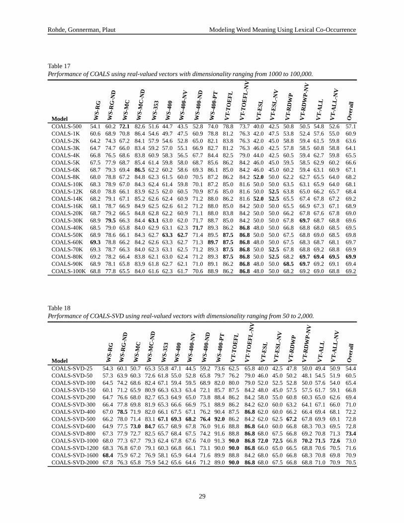
Rohde, Gonnerman, Plaut Modeling Word Meaning Using Lexical Co-Occurrence
Table 17Performance of COALS using real-valued vectors with dimensionality ranging from 1000 to 100,000.
Model WS-
RG
WS-
RG
-ND
WS-
MC
WS-
MC
-ND
WS-
353
WS-
400
WS-
400-
NV
WS-
400-
ND
WS-
400-
PT
VT-
TO
EF
L
VT-
TO
EF
L-N
V
VT-
ESL
VT-
ESL
-NV
VT-
RD
WP
VT-
RD
WP
-NV
VT-
AL
L
VT-
AL
L-N
V
Ove
rall
COALS-500 54.1 60.2 72.1 82.6 51.6 44.7 43.5 52.8 74.0 78.8 73.7 40.0 42.5 50.8 50.5 54.8 52.6 57.1COALS-1K 60.6 68.9 70.8 86.4 54.6 49.7 47.5 60.9 78.8 81.2 76.3 42.0 47.5 53.8 52.4 57.6 55.0 60.9COALS-2K 64.2 74.3 67.2 84.1 57.9 54.6 52.8 65.0 82.1 83.8 76.3 42.0 45.0 58.8 59.4 61.5 59.8 63.6COALS-3K 64.7 74.7 66.0 83.4 59.2 57.0 55.1 66.9 82.7 81.2 76.3 46.0 42.5 57.8 58.5 60.8 58.8 64.1COALS-4K 66.8 76.5 68.6 83.8 60.9 58.3 56.5 67.7 84.4 82.5 79.0 44.0 42.5 60.5 59.4 62.7 59.8 65.5COALS-5K 67.5 77.9 68.7 85.4 61.4 59.8 58.0 68.7 85.6 86.2 84.2 46.0 45.0 59.5 58.5 62.9 60.2 66.6COALS-6K 68.7 79.3 69.4 86.5 62.2 60.2 58.6 69.3 86.1 85.0 84.2 46.0 45.0 60.2 59.4 63.1 60.9 67.1COALS-8K 68.0 78.8 67.2 84.8 62.3 61.5 60.0 70.5 87.2 86.2 84.2 52.0 50.0 62.2 62.7 65.5 64.0 68.2COALS-10K 68.3 78.9 67.0 84.3 62.4 61.4 59.8 70.1 87.2 85.0 81.6 50.0 50.0 63.5 63.1 65.9 64.0 68.1COALS-12K 68.0 78.8 66.1 83.9 62.5 62.0 60.5 70.9 87.6 85.0 81.6 50.0 52.5 63.8 65.0 66.2 65.7 68.4COALS-14K 68.2 79.1 67.1 85.2 62.6 62.4 60.9 71.2 88.0 86.2 81.6 52.0 52.5 65.5 67.4 67.8 67.2 69.2COALS-16K 68.1 78.7 66.9 84.9 62.5 62.6 61.2 71.2 88.0 85.0 84.2 50.0 50.0 65.5 66.9 67.3 67.1 68.9COALS-20K 68.7 79.2 66.5 84.8 62.8 62.2 60.9 71.1 88.0 83.8 84.2 50.0 50.0 66.2 67.8 67.6 67.8 69.0COALS-30K 68.9 79.5 66.3 84.4 63.1 63.0 62.0 71.7 88.7 85.0 84.2 50.0 50.0 67.8 69.7 68.7 68.8 69.6COALS-40K 68.5 79.0 65.8 84.0 62.9 63.1 62.3 71.7 89.3 86.2 86.8 48.0 50.0 66.8 68.8 68.0 68.5 69.5COALS-50K 68.9 78.6 66.1 84.3 62.7 63.3 62.7 71.4 89.5 87.5 86.8 50.0 50.0 67.5 68.8 69.0 68.5 69.8COALS-60K 69.3 78.8 66.2 84.2 62.6 63.3 62.7 71.3 89.7 87.5 86.8 48.0 50.0 67.5 68.3 68.7 68.1 69.7COALS-70K 69.3 78.7 66.3 84.0 62.3 63.1 62.5 71.2 89.3 87.5 86.8 50.0 52.5 67.8 68.8 69.2 68.8 69.9COALS-80K 69.2 78.2 66.4 83.8 62.1 63.0 62.4 71.2 89.3 87.5 86.8 50.0 52.5 68.2 69.7 69.4 69.5 69.9COALS-90K 68.9 78.1 65.8 83.9 61.8 62.7 62.1 71.0 89.1 86.2 86.8 48.0 50.0 68.5 69.7 69.2 69.1 69.4COALS-100K 68.8 77.8 65.5 84.0 61.6 62.3 61.7 70.6 88.9 86.2 86.8 48.0 50.0 68.2 69.2 69.0 68.8 69.2
Table 18Performance of COALS-SVD using real-valued vectors with dimensionality ranging from 50 to 2,000.
Model WS-
RG
WS-
RG
-ND
WS-
MC
WS-
MC
-ND
WS-
353
WS-
400
WS-
400-
NV
WS-
400-
ND
WS-
400-
PT
VT-
TO
EF
L
VT-
TO
EF
L-N
V
VT-
ESL
VT-
ESL
-NV
VT-
RD
WP
VT-
RD
WP
-NV
VT-
AL
L
VT-
AL
L-N
V
Ove
rall
COALS-SVD-25 54.3 60.1 50.7 65.3 55.8 47.1 44.5 59.2 73.6 62.5 65.8 40.0 42.5 47.8 50.0 49.4 50.9 54.4COALS-SVD-50 57.3 63.9 60.3 72.6 61.8 55.0 52.8 65.8 79.7 76.2 79.0 46.0 45.0 50.2 48.1 54.5 51.9 60.5COALS-SVD-100 64.5 74.2 68.6 82.4 67.1 59.4 59.5 68.9 82.0 80.0 79.0 52.0 52.5 52.8 50.0 57.6 54.0 65.4COALS-SVD-150 60.1 71.2 65.9 80.9 66.3 63.3 63.4 72.1 85.7 87.5 84.2 48.0 45.0 57.5 57.5 61.7 59.1 66.8COALS-SVD-200 64.7 76.6 68.0 82.7 65.3 64.9 65.0 73.8 88.4 86.2 84.2 58.0 55.0 60.8 60.3 65.0 62.6 69.4COALS-SVD-300 66.4 77.8 69.8 81.9 65.3 66.6 66.9 75.1 88.9 86.2 84.2 62.0 60.0 63.2 64.1 67.1 66.0 71.0COALS-SVD-400 67.0 78.5 71.9 82.0 66.1 67.5 67.1 76.2 90.4 87.5 86.8 62.0 60.0 66.2 66.4 69.4 68.1 72.2COALS-SVD-500 66.2 78.0 71.4 83.1 67.1 69.3 68.2 76.4 92.0 86.2 84.2 62.0 62.5 67.2 67.8 69.9 69.1 72.8COALS-SVD-600 64.9 77.5 73.0 84.7 65.7 68.9 67.8 76.0 91.6 88.8 86.8 64.0 60.0 66.8 68.3 70.3 69.5 72.8COALS-SVD-800 67.3 77.9 72.7 82.5 65.7 68.4 67.5 74.2 91.6 88.8 86.8 68.0 67.5 66.8 69.2 70.8 71.3 73.4COALS-SVD-1000 68.0 77.3 67.7 79.3 62.4 67.8 67.6 74.0 91.3 90.0 86.8 72.0 72.5 66.8 70.2 71.5 72.6 73.0COALS-SVD-1200 68.3 76.8 67.0 79.1 60.3 66.8 66.1 73.1 90.0 90.0 86.8 66.0 65.0 66.5 68.8 70.6 70.5 71.6COALS-SVD-1600 68.4 75.9 67.2 76.9 58.1 65.9 64.4 71.6 89.9 88.8 84.2 68.0 65.0 66.8 68.3 70.8 69.8 70.9COALS-SVD-2000 67.8 76.3 65.8 75.9 54.2 65.6 64.6 71.2 89.0 90.0 86.8 68.0 67.5 66.8 68.8 71.0 70.9 70.5
29

Rohde, Gonnerman, Plaut Modeling Word Meaning Using Lexical Co-Occurrence
Table 19Performance of COALS-SVDB using binary vectors with dimensionality ranging from 50 to 2,000.
Model WS-
RG
WS-
RG
-ND
WS-
MC
WS-
MC
-ND
WS-
353
WS-
400
WS-
400-
NV
WS-
400-
ND
WS-
400-
PT
VT-
TO
EF
L
VT-
TO
EF
L-N
V
VT-
ESL
VT-
ESL
-NV
VT-
RD
WP
VT-
RD
WP
-NV
VT-
AL
L
VT-
AL
L-N
V
Ove
rall
COALS-SVDB-25 62.4 67.0 50.9 63.7 48.1 42.2 39.6 52.6 71.0 58.8 56.6 28.0 30.0 40.8 40.3 42.4 40.8 49.9COALS-SVDB-50 57.9 63.9 63.2 72.9 53.2 49.4 46.4 60.0 78.3 60.0 57.9 38.0 40.0 46.7 46.5 48.1 47.2 55.5COALS-SVDB-100 63.9 70.1 68.2 79.1 61.6 56.4 55.5 65.0 82.0 78.1 72.4 38.0 40.0 52.3 50.7 55.5 52.2 62.0COALS-SVDB-150 59.8 68.5 67.5 78.7 61.0 58.9 59.0 69.0 85.3 85.0 84.2 50.0 50.0 54.0 53.0 59.3 56.9 64.8COALS-SVDB-200 62.1 72.0 66.6 79.7 59.7 60.4 59.8 69.7 87.0 85.0 84.2 54.0 55.0 56.7 55.6 61.4 59.1 66.1COALS-SVDB-300 63.7 75.0 68.4 78.8 61.0 63.3 63.6 73.0 88.1 86.2 86.8 58.0 60.0 61.8 61.3 65.7 64.3 68.8COALS-SVDB-400 66.6 78.2 75.1 84.2 60.9 64.4 64.4 73.2 89.4 88.8 89.5 60.0 60.0 62.3 63.9 66.7 66.5 70.8COALS-SVDB-500 66.7 76.8 74.6 82.3 61.4 65.2 64.8 73.5 89.6 91.2 92.1 56.0 52.5 64.2 66.0 68.0 67.4 70.8COALS-SVDB-600 64.9 76.4 74.9 82.6 60.0 64.6 65.1 73.3 87.8 88.8 86.8 62.0 57.5 64.2 66.4 68.3 67.8 70.5COALS-SVDB-800 67.2 77.0 73.9 80.2 59.3 64.4 64.6 71.5 87.2 86.2 86.8 70.0 67.5 63.2 64.1 68.0 67.4 70.8COALS-SVDB-1000 66.6 76.6 68.5 79.7 57.7 63.9 64.2 70.5 86.0 86.2 89.5 62.0 62.5 63.2 64.5 67.3 67.8 69.3COALS-SVDB-1200 68.2 76.5 71.9 80.6 54.8 63.4 64.0 69.5 86.7 86.2 89.5 70.0 70.0 65.2 66.4 69.7 70.2 70.4COALS-SVDB-1600 65.0 72.8 71.9 77.7 51.9 61.0 61.1 66.2 84.6 87.5 89.5 68.0 65.0 64.5 65.5 69.2 68.8 68.5COALS-SVDB-2000 65.8 73.0 71.1 77.6 47.4 59.3 59.0 64.7 83.0 88.8 92.1 68.0 70.0 63.5 64.5 68.5 68.8 67.7
12 120 1200Corpus Size (millions of words)
46
48
50
52
54
56
58
60
62
64
66
68
70
Ove
rall
Scor
e
Window Size: 2Window Size: 4Window Size: 7Window Size: 10
Figure 14: Effects of corpus size and ramped window size on the overall weighted score of the COALS-14K model.
30

Rohde, Gonnerman, Plaut Modeling Word Meaning Using Lexical Co-Occurrence
4.4 Corpus and window size
HAL has typically been trained on smaller corpora butwith larger windows than we have used here. In this sec-tion we examine the interaction between corpus size andwindow size on the performance of COALS-14K. Fig-ure 14 shows the overall performance of the model withramped windows ranging from radius 2 to radius 10. Themodels were trained on either our full Usenet corpus or ona random sampling of 10% or 1% of the articles, whichhave approximately 120 million and 12 million words, re-spectively.
Larger windows capture more meaningful co-occurrences, but they also capture more noise. On thesmallest corpus, the best performance is achieved bythe size 10 window because it is able to collect more ofthe precious data. However, with the 120 million-wordcorpus, the signal-to-noise ratio of the largest windowdeclines and the size 7 and size 4 windows performbetter. On the full corpus, the size 4 window is the best,followed by the size 2 window and the largest window isactually the worst. Therefore, there is a clear tradeoff toconsider in choosing an appropriate window for use withthe HAL or COALS methods. Smaller corpora demandlarger windows and larger corpora demand smaller ones.
5 Discussion
We have introduced a new method for deriving wordmeanings, in the form of high-dimensional vectors, fromlarge, unlabeled text corpora. Our method, COALS, andespecially its lower-dimensional variant, COALS-SVD,performed well in comparison to 11 other models on a va-riety of empirical tests. It was particularly effective in pre-dicting human similarity judgments on our WS-400 task,which included a greater diversity of word-pair types thandid previous experiments.
The only other model to perform as well as COALS wasthat based on Roget’s Thesaurus (Jarmasz & Szpakowicz,2003). However, ROGET, like the WordNet models, suf-fers from several drawbacks. Principal among these is thefact that these models rely on structured lexicons result-ing from years of expert human labor, and cannot there-fore easily be extended to larger vocabularies or other lan-guages. The HAL, LSA, and COALS models, on the otherhand, can be applied to any language for which sufficienttext is available. Also, the WordNet and Roget modelsdo not produce semantic representations that can easilybe used in a cognitive model (although see Powell, Za-jicek, and Duce (2000) for one attempt at this). A princi-pal advantage of the WordNet and Roget’s models is thatthey distinguish word senses. More work needs to be donein automatic word-sense clustering and disambiguation toallow the vector-based methods to do this.
Our model originated as a replication of HAL (Lund& Burgess, 1996), and it continues to be similar to HALboth in its applicability and in the basic premise that hu-man knowledge of lexical semantics can, to a certain ex-tent, be represented as high-dimensional vectors learnedthrough exposure to language alone. Although COALS-SVD achieves better results using fewer dimensions, wehave reported several analyses of the plain COALS modelbecause of its analogy to HAL. As we have shown, the im-proved normalization function used in our method, alongwith the other less significant changes, results in a muchmore effective methodology.
In our tests, LSA also performed much better thanHAL, although not quite as well as COALS, particularlyon the vocabulary tests. COALS-SVD and LSA bothmake use of the singular value decomposition. One differ-ence between the two models is their normalization pro-cedures, but a more fundamental difference is the form ofthe co-occurrence matrix they construct. LSA assumesthat the input is a discrete set of (usually small) docu-ments. COALS, on the other hand, like HAL, makes useof an undifferentiated text corpus, using a moving windowto define the collocation of words. As a result, the modelswill scale up differently with more data. The number ofcolumns in the LSA matrix is proportional to the numberof documents. Although the SVD can be computed onmatrices with millions of rows and columns, that is onlypossible with special machinery and with very sparse ma-trices. Therefore, it may not be possible to run LSA onvery large document collections without discarding all buta small excerpt from each document.
On the other hand, the size of the matrix used inCOALS-SVD is essentially fixed. In this work, we used amatrix with 15,000 rows and 14,000 columns. If the sizeof the training corpus were increased by several orders ofmagnitude, the size of this matrix need not change. Itsdensity would increase and a slightly larger matrix mightbe preferable with additional data, but it should still bepossible to implement the COALS-SVD method on a sin-gle personal computer. Therefore, COALS-SVD shouldscale up more easily than LSA to corpora much larger thaneven our 1.2 billion-word text.
Real-valued and binary COALS-SVD vectors can beaccessed on the web at:
http://tedlab.mit.edu/∼dr/COALS/
ReferencesBanerjee, S., & Pedersen, T. (2002). An adapted lesk algorithm
for word sense disambiguation using WordNet. In Pro-ceedings of the third international conference on intelli-gent text processing and computational linguistics. Mex-ico City.
Berry, M., Do, T., O’Brien, G., Krishna, V., & Varadhan, S.
31

Rohde, Gonnerman, Plaut Modeling Word Meaning Using Lexical Co-Occurrence
(1996). Svdpackc (version 1.0) user’s guide (Tech. Rep.No. Tech. Report CS-93-194). Univ. of Tennessee.
Budanitsky, A., & Hirst, G. (2001). Semantic distance in word-net: An experimental, application-oriented evaluation offive measures. In Workshop on wordnet and other lex-ical resources, in the north american chapter of the as-sociation for computational linguistics. Pittsburgh, PA:NAACL-2000.
Burgess, C. (1998). From simple associations to the buildingblock of language: Modeling meaning in memory withthe HAL model. Behavior Research Methods, Instru-ments, and Computers, 30, 188-198.
Burgess, C., & Lund, K. (1997a). Modelling parsing con-straints with high-dimensional context space. Languageand Cognitive Processes, 12(2/3), 177–210.
Burgess, C., & Lund, K. (1997b). Representing abstract wordsand emotional connotation in a high-dimensional mem-ory space. In Proceedings of the 19th annual conferenceof the Cognitive Science Society (pp. 61–66). Mahwah,NJ: Lawrence Erlbaum Associates.
Deerwester, S. C., Dumais, S. T., Furnas, G. W., Landauer, T. K.,& Harshman, R. A. (1990). Indexing by latent semanticanalysis. Journal of the American Society of InformationScience, 41, 391–407.
Finkelstein, L., Gabrilovich, E., Matias, Y., Rivlin, E., Solan,Z., Wolfman, G., & Ruppin, E. (2002). Placing searchin context: The concept revisited. ACM Transactions onInformation Systems, 20(1), 116–131.
Foltz, P. W., Kintsch, W., & Landauer, T. K. (1998). Themeasurement of textual coherence with Latent SemanticAnalysis. Discourse Processes, 25, 285–307.
Hinton, G. E., & Shallice, T. (1991). Lesioning an attractor net-work: Investigations of acquired dyslexia. PsychologicalReview, 98, 74–95.
Hirst, G., & St-Onge, D. (1998). Lexical chains as repre-sentations of context for the detection and correction ofmalapropisms. In C. Fellbaum (Ed.), Wordnet: An elec-tronic lexical database (pp. 305–332). Cambridge, MA:The MIT Press.
Jarmasz, M., & Szpakowicz, S. (2003). Roget’s Thesaurus andsemantic similarity. In Proceedings of the conference onrecent advances in natural language processing (ranlp2003) (pp. 212–219). Borovets, Bulgaria.
Jiang, J. J., & Conrath, D. W. (1997). Semantic similarity basedon corpus statistics and lexical taxonomy. In Proceedingsof the 10th international conference on research in com-putational linguistics (rocling x) (pp. 19–33). Taiwan:Academica Sinica.
Johnson, S. (1967). Hierarchical clustering schemes. Psychome-trika, 2, 241–254.
Kawamoto, A. H. (1993). Nonlinear dynamics in the resolutionof lexical ambiguity: A parallel distributed processing ac-count. Journal of Memory and Language, 32, 474–516.
Kintsch, W. (2000). Metaphor comprehension: A computationaltheory. Psychonomic Bulletin and Review, 7, 257–266.
Kruskal, J. B. (1964). Multidimensional scaling by optimizinggoodness of fit to a nonmetric hypothesis. Psychometrika,29, 1–27.
Kucera, H., & Francis, W. N. (1967). Computational analysisof present-day American English. Providence, RI: BrownUniversity Press.
Laham, D. (1971). Latent semantic analysis approaches to cate-gorization. In Proceedings of the 19th annual conferenceof the Cognitive Science Society (p. 979). Mahwah, NJ:Lawrence Erlbaum Associates.
Landauer, T. K., & Dumais, S. T. (1997). A solution to plato’sproblem: The Latent Semantic Analysis theory of acqui-sition, induction, and representation of knowledge. Psy-chological Review, 104, 211–240.
Landauer, T. K., Foltz, P. W., & Laham, D. (1998). An introduc-tion to Latent Semantic Analysis. Discourse Processes,25, 259–284.
Leacock, C., & Chodorow, M. (1998). Combining local con-text and wordnet similarity for word sense identifica-tion. In C. Fellbaum (Ed.), Wordnet: An electronic lexi-cal database (pp. 265–283). Cambridge, MA: The MITPress.
Lesk, M. (1986). Automatic sense disambiguation usingmachine-readable dictionaries: How to tell a pine conefrom an ice cream cone. In Proceedings of sigdoc ’86(pp. 24–26). Toronto.
Levin, B. (1993). English verb classes and alternations: Apreliminary investigation. Chicago, IL: The Universityof Chicago Press.
Lin, D. (1997). Using syntactic dependency as a local contextto resolve word sense ambiguity. In Proceedings of the35th annual meeting of the association for computationallinguists (pp. 64–71). Madrid.
Lund, K., & Burgess, C. (1996). Producing high-dimensionalsemantic spaces from lexical co-occurrence. Behav-ior Research Methods, Instruments, and Computers, 28,203–208.
Lund, K., Burgess, C., & Atchley, R. A. (1995). Seman-tic and associative priming in high-dimensional semanticspace. In Proceedings of the 17th annual conference ofthe Cognitive Science Society (pp. 660–665). Mahwah,NJ: Lawrence Erlbaum Associates.
Lund, K., Burgess, C., & Audet, C. (1996). Dissociatingsemantic and associative word relationships using high-dimensional semantic space. In Proceedings of the 18thannual conference of the Cognitive Science Society (pp.603–608). Mahwah, NJ: Lawrence Erlbaum Associates.
McDonald, S., & Lowe, W. (1998). Modelling functional prim-ing and the associative boost. In Proceedings of the 20thannual conference of the Cognitive Science Society (pp.675–680). Mahwah, NJ: Lawrence Erlbaum Associates.
Miller, G., Beckwith, R., Fellbaum, C., Gross, D., & Miller,K. (1990). Introduction to wordnet: an online lexicaldatabase. International Journal of Lexicography, 3(4),235–244.
32

Rohde, Gonnerman, Plaut Modeling Word Meaning Using Lexical Co-Occurrence
Miller, G. A., & Charles, W. G. (1991). Contextual correlates ofsemantic similarity. Language and Cognitive Processes,6(1), 1–28.
Patwardhan, S., Banerjee, S., & Pedersen, T. (2003). Usingmeasures of semantic relatedness for word sense disam-biguation. In Proceedings of the fourth international con-ference on intelligent text processing and computationallinguistics, february 17–21. Mexico City.
Plaut, D. C. (1997). Structure and function in the lexical sys-tem: Insights from distributed models of word readingand lexical decision. Language and Cognitive Processes,12, 767–808.
Plaut, D. C., & Booth, J. R. (2000). Individual and develop-mental differences in semantic priming: Empirical andcomputational support for a single-mechanism account oflexical processing. Psychological Review, 107, 786–823.
Plaut, D. C., Seidenberg, M. S., McClelland, J. L., & Patter-son, K. (1996). Understanding normal and impairedword reading: computational principles in quasi-regulardomains. Psychological Review, 103, 56–115.
Powell, C., Zajicek, M., & Duce, D. (2000). The generation ofword meanings from dictionaries. In Icslp 2000, vol. iii(pp. 482–485). Beijing.
Rada, R., Mili, H., Bicknell, E., & Blettner, M. (1989). Develop-ment and application of a metric on semantic nets. IEEETransactions on Systems, Man and Cybernetics, 19(1),17–30.
Ramscar, M. (2001). The influence of semantics on past-tenseinflection. In Proceedings of the 23rd annual conferenceof the Cognitive Science Society (pp. 809–814). Mahwah,NJ: Lawrence Erlbaum Associates.
Resnick, P. (1995). Using information content to evaluate se-mantic similarity. In Proceedings of the 14th interna-tional joint conference on artificial intelligence (pp. 448–453). Montreal.
Rohde, D. L. T. (2002a). A connectionist model of sentence com-prehension and production. Unpublished doctoral disser-tation, Carnegie Mellon University, Department of Com-puter Science, Pittsburgh, PA.
Rohde, D. L. T. (2002b). Methods for binary multidimensionalscaling. Neural Computation, 14, 1195–1232.
Rubenstein, H., & Goodenough, J. B. (1965). Contextual corre-lates of synonymy. Communications of the ACM, 8(10),627–633.
Shepard, R. N. (1962). The analysis of proximities: Multi-dimensional scaling with an unknown distance function.Psychometrika, 27, 125–139, 219–246.
Turney, P. D. (2001). Mining the web for synonyms: PMI-IR vsLSA on TOEFL. In Proceedings of the twelfth europeanconference on machine learning (ecml-2001) (pp. 491–502). Freiburg, Germany.
Wu, Z., & Palmer, M. (1994). Verb semantics and lexical selec-tion. In Proceedings of the 32nd annual meeting of theassociation for computational linguistics. Las Cruces,Mew Mexico.
33