Embed Size (px)
Citation preview
An Improved Long-Run Model for Multiple Warehouse LocationAuthor(s): Dennis J. Sweeney and Ronad L. TathamSource: Management Science, Vol. 22, No. 7 (Mar., 1976), pp. 748-758Published by: INFORMSStable URL: http://www.jstor.org/stable/2630159Accessed: 17/11/2009 14:26
Your use of the JSTOR archive indicates your acceptance of JSTOR's Terms and Conditions of Use, available athttp://www.jstor.org/page/info/about/policies/terms.jsp. JSTOR's Terms and Conditions of Use provides, in part, that unlessyou have obtained prior permission, you may not download an entire issue of a journal or multiple copies of articles, and youmay use content in the JSTOR archive only for your personal, non-commercial use.
Please contact the publisher regarding any further use of this work. Publisher contact information may be obtained athttp://www.jstor.org/action/showPublisher?publisherCode=informs.
Each copy of any part of a JSTOR transmission must contain the same copyright notice that appears on the screen or printedpage of such transmission.
JSTOR is a not-for-profit service that helps scholars, researchers, and students discover, use, and build upon a wide range ofcontent in a trusted digital archive. We use information technology and tools to increase productivity and facilitate new formsof scholarship. For more information about JSTOR, please contact [email protected].
INFORMS is collaborating with JSTOR to digitize, preserve and extend access to Management Science.
http://www.jstor.org
MANAGEMENT SCIENCE Vol. 22, No. 7, March, 1976
Printed in USA.
AN IMPROVED LONG-RUN MODEL FOR MULTIPLE WAREHOUSE LOCATION*
DENNIS J. SWEENEY AND RONAD L. TATHAMt
University of Cincinnati
This paper proposes an improved model for solving the long-run multiple warehouse location problem. The approach used provides a synthesis of a mixed integer programming formulation for the single-period warehouse location model with a dynamic programming procedure for finding the optimal sequence of configurations over multiple periods. We show that only the Rt best rank order solutions in any single period need be considered as candidates for inclusion in the optimal multi-period solution. Thus the computational feasibility of the dynamic programming procedure is enhanced by restricting the state space to these Rt best solutions. Computational results on the ranking procedure are presented, and a problem involving two plants, five warehouses, 15 customer zones, and five periods is solved to illustrate the application of the method.
1. Introduction
A problem commonly faced in the management of distribution systems is that of determining a set of geographical warehouse locations such that demand is satisfied and a satisfactory level of customer service is maintained with a minimum total distribution cost over a relatively long planning period with varying levels of demand over the period. Various criteria have been suggested for a satisfactory solution procedure to the problem posed [9].
Apparently a good solution procedure for locating warehouses should meet these objectives:
1. be capable of evaluating a reasonable number of possible warehouse configura- tions to determine how many there should be and where they should be located;
2. be capable of evaluating warehouse configurations over time and hence indicat- ing when it is desirable to change configurations in response to shifting demand patterns, supply costs, etc.;
3. allow for interdependence in costs among the warehouse sites during a single period and across multiple periods; i.e., the sites cannot be selected independently of one another nor of the sites chosen in other planning periods;
4. cope with nonlinearities due to both the fixed costs associated with alternative configurations and the variable costs associated with the system throughput;
5. be computationally feasible and efficient. Both static and dynamic procedures have been used to find solutions meeting some,
but not all, of the above criteria. Static warehouse location models deal with the single period problem of finding the optimal warehouse configuration at a particular point in time [3], [4], [8], [10], [14]. These models have experienced varying degrees of success in meeting objectives 1, 3, 4 and 5 above, but simply ignore 2. For this reason they may be suboptimal over a longer planning horizon. Even in the short run, these models ignore the interdependence with the previous planning period. It is implicitly assumed that the existing configuration can be immediately redesigned to implement the optimal solution. However, in many practical problems, by the time the static solution can be implemented it is no longer optimal.
* Processed by Professor Warren H. Hausman, Departmental Editor for Logistics; received September 1973; revised March 1974 and January 1975. This paper has been with the authors 7 months for revision.
t This research was supported by a grant from the George A. Ramlose Foundation, Inc.
748 Copyright C) 1976, The Institute of Management Sciences

IMPROVED LONG-RUN MODEL FOR MULTIPLE WAREHOUSE LOCATION 749
One approach to finding a solution that satisfies criteria 2 and 3 is a multiperiod model proposed by Ballou [2] which employs a heuristic solution procedure based on dynamic programming.' In this procedure, the number of alternative locations consid- ered in each period is equal to T, where T is the number of periods in the planning horizon. The T alternatives considered are the optimal solutions to the static warehouse location problem (SWLP) for each of the T periods. These T alternatives are generated by any of the static models referenced earlier, and are evaluated in each of the other periods providing T distinct alternative configurations for each period. One then chooses by dynamic programming that sequence from these T configura- tions which minimizes the total cost of operation and relocation. However, Ballou's approach is limited since it can only guarantee suboptimal solutions. This is because there is no guarantee that the long-run optimal solution will be composed of a sequence of configurations derived only from static optimal solutions. For example, a configuration which yielded the second best static solution in each planning period could quite possibly yield the long-run optimal location since no relocation costs would be necessary over the planning horizon.
Lodish has pointed out [12], for large practical problems, it is not computationally feasible to consider in a dynamic programming procedure all of the existing warehouse configurations in each period. Ballou's approach overcomes this computa- tional difficulty by the heuristic approach of limiting the number of configurations considered in each period to the optimal static solutions in each of the T periods. In the next section, we show how an optimal multiperiod solution can be obtained by limiting the number of alternatives considered in each period to the R, best rank order (ranked from lowest to highest) static configurations for that period. This preserves the computational feasibility of the dynamic programming approach without resorting to suboptimal solutions. In the following section we show how these R, best solutions can be found as an extension of the solution procedure for the static model.
2. The Multiperiod Model
In Table 1 each column represents a stage (period) in the process and the entries in these columns represent the values the state variable (the single-period warehouse configuration) may take on. The values of these static solutions in each period (column entries) are presented in rank order. Given that these entries are the only alternative solutions considered (we show shortly that it is not necessary to consider any others) the optimal long-run solution may be found by using dynamic program- ming to find the minimum cost path through the matrix, taking into consideration at each stage the costs of moving from one warehouse configuration to any other.
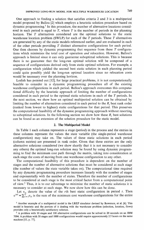
The computational feasibility of this procedure is dependent on the number of stages and the number of alternative solutions that must be considered at each stage (the number of values the state variable takes on). The computational time required by any dynamic programming procedure increases linearly with the number of stages and exponentially with the number of states. Therefore the number of configurations to be considered at each stage is the most critical factor from a computational point of view.2 Thus, it is to our advantage to minimize the number of static solutions it is necessary to consider at each stage. We now show how this can be done.
Let vtr denote the value of the rth best static configuration in period t. Then vinf = T_ v is the sum of the minimum cost warehouse configurations for the entire
l Another example of a multiperiod model is the LREP simulator devised by Bowersox, et al. [6]. This model is heuristic and the portion of it dealing with the warehouse problem (selection, location, flows) provides only a heuristically satisfactory solution.
2 A problem with 10 stages and 100 alternative configurations can be solved in 20 seconds on an IBM 7094. A problem with 50 stages and 1000 configurations would require approximately 2.5 hours on the same machine [13, p. 77].

750 DENNIS J. SWEENEY AND RONALD L. TATHAM
TABLE 1
R, Best Solutions to the Static Warehouse Location Problem by Planning Period
Rank Order Solutions Period (low to
high cost) 1 2 3 ... T
I Viil V21 V31 . .. VT
2 V 12 V22 V32
3 V13 * V33---. * * V34...
v2R2 .
VTRT
VIR,
R, V3R3
planning horizon. (v1l is the least cost static solution in period t). Since no relocation expenses are considered, vinf is a lower bound on the value of the optimal multiperiod solution. If the same configuration was optimal for each period, this would obviously be the optimal multiperiod solution.
Let v* be an upper bound corresponding to any feasible solution to the multiperiod problem. The following theorem can be used to determine how many static solutions it is necessary to rank in each period.
THEOREM. Let K= v* -v inf. Also let R, be such that vR v,- l K and Vt R +I -Vt I > K. In period t, no static solution with value vTr may become part of an optimal multiperiod solution if r > Rt.
PROOF. Suppose r > RT. The value of the best multiperiod solution containing the rth best configuration in year t is bounded below by Et 7, TvT + vTr. Now,
T v +V v + vm -
VT, > vinf + K= v*. t I t t= I
We see from the theorem that K is the maximum possible improvement that can be made over the solution corresponding to v*. Thus it is only necessary to consider the
R, best static solutions in each period for possible inclusion in an optimal multiperiod solution. This results in a state space reduction and makes dynamic programming a feasible solution procedure for practical sized problems.
The values of the R, best configurations for each period are the entries in Table 1. It is important to note that a particular static solution may be considered in one period, and not another, since in general a particular warehouse configuration will not have the same rank in any two periods and the same number of alternatives are not considered in each period; i.e., Ri is not necessarily equal to Rj.
Since the number of static solutions it is necessary to rank in each period depends upon K, it is desirable to have a good upper bound, v*, available. Any feasible solution, such as maintaining the current configuration over the entire planning period, can be used to determine an initial value for v*. Better upper bounds can be generated as the solution procedure progresses. We recommend the following approach. Using the initial value for v*, rank order the P1 best solutions in each period where F, S R,. This may be some preset number of solutions, say 50, or we

IMPROVED LONG-RUN MODEL FOR MULTIPLE WAREHOUSE LOCATION 751
may rank order solutions until v,, t - vt, 1 > constant. In the former case P, will be fixed across periods and in the latter P, will vary. A new (and hopefully better) upper bound can then be generated by using dynamic programming to find the multiperiod solution considering as alternatives in each period the P, best static solutions. This new upper bound is clearly a feasible solution and if it consists of a sequence of optimal static solutions it is the Ballou solution [2]. Using the new value for v* we can recompute K = v* -vinf. If now v - vt, > K for all periods we are finished, and v* is the value of the optimal multiperiod solution. If not, more solutions must be rank ordered in those periods where vt P - vt, I < K.
Ideally one would initially choose P, so that exactly the right number of static solutions was rank ordered the first time through. Unfortunately the right number, P, is data dependent and there is no way to predict this in advance. The most we can hope for is that knowledge of the firm's distribution system will allow a judicious choice. Since the maximum possible improvement from further ranking is given by I = max (K-Vt pt + vt 1, 0) t E ( 1, 2, . ., T}, one might choose to terminate if I was sufficiently small. The value of I is a measure of the maximum possible opportunity loss associated with implementing the solution associated with v*.
3. Finding the R, Best Solutions
Since our dynamic programming procedure depends critically on finding the R, best static solutions for the short-run problem, it is important that the static warehouse location model used be such that this information can easily be obtained. We show here how this information can be obtained when a mixed integer programming formulation of the static problem is employed. For notational convenience we restrict our attention here to a static model for a single commodity class. For an extension to multiple commodity classes we refer the reader to the excellent article by Geoffrion and Graves [8].
The static warehouse location problem may be formulated as the following mixed integer linear program.
I J M J
mi> n E (A + Bjm + C,)xqjm + E Fjz z-O, 1 i=1 =1 J1
I J
s Et EY xijm = Qm m j- 1, 25, ... ., M
(SWLP) 1=1 j=1
i= m XJ
where: xijm =the quantity of goods shipped from factory i (i = 1, ... , I) through
warehouse ] (j = 1, . . ., J) to customer m (m = 1, . .. , M),
Au = per unit cost of shipping from factory i to warehouse j, B;m = per unit cost of shipping from warehouse j to customer m,
Cj =per unit variable cost of storing and handling goods at warehouse j, Fj =fixed cost of operating warehouse j,
Qm = the demand for customer m, Si = the capacity at factory i, and
Wj = the capacity at warehouse j. z=0 if warehouse j closed
= 1 if warehouse j open.

752 DENNIS J. SWEENEY AND RONALD L. TATHAM
Here we have formulated the static warehouse location problem as one of minimiz- ing total distribution costs subject to the usual capacity restrictions on the warehouses and factories, and the constraint that demand must be satisfied. Note that in this model the nonlinearities due to the fixed costs have been included but that we have assumed that transportation and variable warehouse costs are linear. Also note as in [8] that additional linear configuration constraints involving the binary z variables may be included. In addition, the model may be expanded to consider alternative plant locations by introducing another binary variable hi. The second constraint then becomes
J M
I xim <_ Si hi i =- 1, 2. ... I j=I m=1
and an additional term must be added to the objective function to reflect the fixed costs of the various plant locations. Customer service constraints may also be incorporated by adding a constraint of the form
I J M
d amXu,,n/ Qm < D i=1j=1 m=1
where dam is the distance from warehouse j to customer m and D is the firm's desired bound on average delivery distance. The addition of these constraints requires a slight modification of the static solution procedure we are about to present (see [7], [11]).
Benders partitioning procedure [5], [7], [8], [11] has been applied to solve variations of the above mixed integer formulation. We have used the following specialized version of Benders partitioning procedure to obtain the best solution to problem (SWLP) and then applied a simple modification to obtain higher rank order solutions.
Step 0. (Iteration 0.) Pick an arbitrary feasible configuration zo (i.e., such that constraint (2) below is satisfied). Set the lower bound LB equal to - cc and go to step 2.
Step 1. (Iteration N.) Solve problem (IP) below for a (possibly) new configuration. min v
y; z=0, 1I
J I M
s.t. y> E (FQ- W)Vn)zj- Siu/- QmV n =O, ,...,N- 1 (1) (IP) i=l i-l m=1
WjZ > Qm (2) j=l m=l
Denote by (yN, ZN) the optimal solution. Set the lower bound, LB, equal to yN and go to step 2.
Step 2. Solve the primal linear program (LP) below obtained by fixing z at zN and record the values of all the dual variables tjN , Vm. These will be used to generate a new constraint of form (1) above for problem (IP). Assuming I = 1Si > Em= Qm, (LP) must be feasible because of constraint (2) on (IP).
I J M
mini 1E1 JE E1 (Ai + Bjm + Cj)XUm x =1 ]=1 In=
I J
s.t. E E x -Qm m = 1, 2, . ,M (LP) 1
l -l
E EY .. xijm < Si i = 1, 2,. ,I j=l m=lI
I M
'i EY' X;m ?W;Vz;N j-1, 2, ...,J. i= 1 rn=1I
IMPROVED LONG-RUN MODEL FOR MULTIPLE WAREHOUSE LOCATION 753
Denote by (xN} the optimal solution and r(xN) its value. Set the upper bound UB = r(xN) + EJ 1FizN and go to step 3.
Step 3. If UB - e < LB, stop. The optimal solution is given by (zN, x N). If not, set N= N + 1 and go to step 1.
Once the optimal static solution has been found using the above algorithm, the second best solution can be found by adding a constraint to (IP), resetting UB = 00 and continuing with step 1. The constraint added is one developed by Balas and Jeroslow [1] for making canonical cuts on the unit hypercube.
E z; - E z; < N(q)-1 (3) j (-O, j (-C,
where
01 = (j Zj = 1 in the best solution);
Cl = {j Zj=0 in the best solution);
N(01) = number of elements in 01.
This cut, see [1], will make infeasible the best solution but no others. The optimal solution after constraint (3) has been added is the second best solution. Another constraint of the form (3) is then added, and so on, until the R, best solutions have been obtained.
Once 'the optimal solution has been obtained successive solutions can be ranked in considerably less time. We have obtained computational results on an IBM 370/168 for sixteen years of data on problems involving two plants, five warehouse locations, and 15 customer zones. These results are summarized in Table 2. An average of 6.9
TABLE 2
Computational Results for Sixteen Years of Data for Two Plants, Five Warehouse Locations, and Fifteen Customer Zones
Optimal Solution Higher Ranked Solutions Average No.
No. of of Benders' Average CPU No. of Benders' CPU Seconds Solutions Iterations Seconds per
Year Iterations per Solution Ranked per solution Solution
1 15 34.5 19 1.5 3.4 2 17 39.6 19 1.2 2.8 3 6 12.0 12 1.8 3.7 4 5 10.1 12 1.8 3.7 5 4 16.7 12 1.8 7.6 6 5 18.3 12 1.6 3.7 7 7 11.7 12 2.0 3.3 8 3 5.1 12 2.3 3.8 9 8 16.1 12 1.9 3.9
10 8 12.5 12 2.1 3.3 1 1 3 4.2 12 2.4 3.4 12 7 12.7 1 1 2.2 4.3 13 5 10.7 12 1.8 3.9 14 7 15.4 12 1.6 3.7 15 3 7.2 19 1.9 4.5 16 7 16.1 19 1.8 4.2
Averages 6.9 15.2 1.9 3.9
754 DENNIS J. SWEENEY AND RONALD L. TATHAM
Benders iterations, each involving the solution of (IP) and (LP) once, were required to find the 16 optimal solutions. An average of 1.9 Benders iterations were required in going from the rth to the (r + 1) best solution for 219 rankings over the sixteen years of data. Approximately 28% of the computational work required to find an optimal solution was required to rank solutions. The amount of computer execution time needed is obviously a function of the efficiency of the subroutines used to solve (IP) and (LP). We do not consider our code to be efficient, but for the 16 years of data the average CPU time to find the optimal solution was 15.2 seconds. The average CPU time for ranking was 3.9 seconds per solution.
Geoffrion and Graves [8] have reported computer execution times ranging up to approximately three minutes on an IBM 360/91 for finding the optimal solution to a quite large multicommodity problem using Benders decomposition. Based on our results (approximately 28% computational effort), it would appear that a reasonable number of configurations can be ranked using our approach even for very large problems. We note also that the ability to rank order a reasonable number of alternatives is often of interest even when it is only desired to solve the static problem.
4. An Illustrative Application
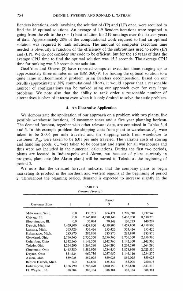
We demonstrate the application of our approach on a problem with two plants, five possible warehouse locations, 15 customer zones and a five year planning horizon. The demand forecast, together with other relevant data, are contained in Tables 3, 4 and 5. In this example problem the shipping costs from plant to warehouse, Aij, were taken to be 8.006 per mile traveled and the shipping costs from warehouse to customer, Bj,,?, were taken to be $.01 per mile traveled. The variable costs of storing and handling goods, Cj, were taken to be constant and equal for all warehouses and thus were not included in the numerical calculations. During the first two periods, plants are located in Indianapolis and Akron, but because of plans currently in progress, plant one (the Akron plant) will be moved to Toledo at the beginning of period 3.
We note that the demand forecast indicates that the company plans to begin marketing its product in the northern and western regions at the beginning of period 2. Throughout the planning period, demand is expected to increase slightly in the
TABLE 3
Demand Forecasts
Period
Customer Zone 1 2 3 4 5
Milwaukee, Wisc. 0.0 433,235 866,471 1,299,710 1,732,940
Chicago, Ill. 0.0 2,145,070 4,290,140 6,435,200 8,580,270
Bloomington, Ill. 0.0 35,074 70,148 105,223 140,297 Detroit, Mich. 4,459,800 4,459,800 4,459,800 4,459,800 4,459,800
Lansing, Mich. 353,426 353,426 353,426 353,426 353,426 Kalamazoo, Mich. 283,870 283,870 283,870 283,870 283,870 Cleveland, Ohio 2,756,360 2,756,360 2,756,360 2,756,360 2,756,360 Columbus, Ohio 1,142,360 1,142,360 1,142,360 1,142,360 1,142,360
Toledo, Ohio 1,264,290 1,264,290 1,264,290 1,264,290 1,264,290
Cincinnati, Ohio 1,445,380 1,589,920 1,734,450 1,878,990 2,023,530
Dayton, Ohio 881,624 969,786 1,057,950 1,146,110 1,234,270
Akron, Ohio 859,025 859,025 859,025 859,025 859,025 Benton Harbor, Mich. 0.0 62,668 125,337 188,005 250,673
Indianapolis, Ind. 1,166,790 1,283,470 1,400,150 1,156,830 1,633,510 Ft. Wayne, Ind. 388,384 388,384 388,384 388,384 388,384
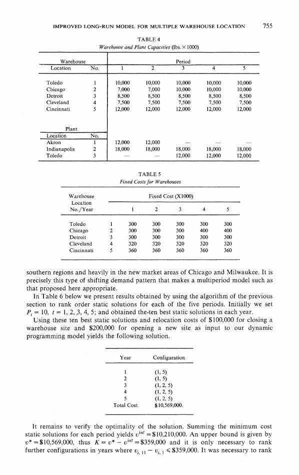
IMPROVED LONG-RUN MODEL FOR MULTIPLE WAREHOUSE LOCATION 755
TABLE 4
Warehouse and Plant Capacities (lbs. x 1000)
Warehouse Period Location No. 1 2 3 4 5
Toledo 1 10,000 10,000 10,000 10,000 10,000 Chicago 2 7,000 7,000 10,000 10,000 10,000 Detroit 3 8,500 8,500 8,500 8,500 8,500 Cleveland 4 7,500 7,500 7,500 7,500 7,500 Cincinnati 5 12,000 12,000 12,000 12,000 12,000
Plant Location No. Akron 1 12,000 12,000 Indianapolis 2 18,000 18,000 18,000 18,000 18,000 Toledo 3 - 12,000 12,000 12,000
TABLE 5 Fixed Costs for Warehouses
Warehouse Fixed Cost (X1000) Location
No./Year 1 2 3 4 5
Toledo 1 300 300 300 300 300 Chicago 2 300 300 300 400 400 Detroit 3 300 300 300 300 300 Cleveland 4 320 320 320 320 320 Cincinnati 5 360 360 360 360 360
southern regions and heavily in the new market areas of Chicago and Milwaukee. It is precisely this type of shifting demand pattern that makes a multiperiod model such as that proposed here appropriate.
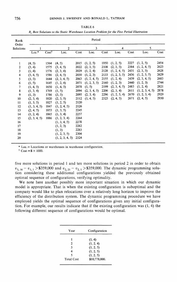
In Table 6 below we present results obtained by using the algorithm of the previous section to rank order static solutions for each of the five periods. Initially we set Pt = 10, t = 1, 2,,3, 4, 5; and obtained the-ten best static solutions in each year.
Using these ten best static solutions and relocation costs of $100,000 for closing a warehouse site and S200,000 for opening a new site as input to our dynamic programming model yields the following solution.
Year Configuration
1 (1,5) 2 (1, 5) 3 (1,2,5) 4 (1,2,5) 5 (1,2,5)
Total Cost $10,569,000.
It remains to verify the optimality of the solution. Summing the minimum cost static solutions for each period yields vinf = $10,210,000. An upper bound is given by v* = S10,569,000, thus K = v* - vinf=S359,000 and it is only necessary to rank further configurations in years where v1 1-Vt, l < $359,000. It was necessary to rank
756 DENNIS J. SWEENEY AND RONALD L. TATHAM
TABLE 6
Rt Best Solutions to the Static Warehouse Location Problem for the Five Period Illustration
Rank Period Order
Solutions 1 2 3 4 5 Loc.* Costt Loc. Cost Loc. Cost Loc. Cost Loc. Cost
1 (4, 5) 1564 (4, 5) 2015 (1, 2, 5) 1950 (1, 2, 5) 2227 (1, 2, 5) 2454 2 (3, 4) 1575 (3, 4, 5) 2022 (2, 3, 5) 2108 (2, 3, 5) 2384 (1, 2, 4, 5) 2623 3 (1, 4) 1576 (2,3, 4) 2029 (1, 2,4) 2128 (1, 2,4, 5) 2431 (2,3, 5) 2628 4 (3, 4, 5) 1586 (2, 4, 5) 2030 (1, 2, 3) 2133 (1, 2, 3, 5) 2436 (1, 2, 3, 5) 2629 5 (3, 5) 1644 (2, 3, 4, 5) 2063 (1, 2, 4, 5) 2155 (1, 2, 4) 2439 (2,;3, 4, 5) 2683 6 (1, 5) 1645 (1, 2, 4) 2071 (1, 2, 3, 5) 2160 (1, 2, 3) 2440 (1, 2, 3) 2744 7 (1, 4, 5) 1650 (1, 4, 5) 2078 (1, 5) 2199 (2, 3, 4, 5) 2483 (1, 2, 4) 2821 8 (1, 3, 4) 1769 (1, 5) 2094 (2, 3, 4, 5) 2206 (2, 3, 4) 2611 (1, 2, 3, 4, 5) 2878 9 (1, 3) 1786 (3, 5) 2095 (2, 3, 4) 2296 (1, 2, 3, 4) 2670 (1, 2, 3, 4) 2929
10 (2, 3, 4) 1820 (2, 3, 5) 2112 (1, 4, 5) 2323 (2, 4, 5) 2671 (2, 4, 5) 2930 11 (1,3,5) 1827 (1,2,5) 2120 12 (1, 3, 4, 5) 1847 (1, 2, 4, 5) 2126 13 (2, 4, 5) 1853 (1, 3, 5) 2245 14 (1, 2, 4) 1865 (1, 3, 4) 2257 15 (2, 3, 4, 5) 1886 (1, 2, 3, 4) 2264 16 (1, 3, 4, 5) 2278 17 (1, 2, 3) 2282 18 (1, 3) 2283 19 (1, 2, 3, 5) 2304 20 (1, 2, 3, 4, 5) 2324
* Loc.= Locations or warehouses in warehouse configuration. t Cost = $ x 1000.
five more solutions in period 1 and ten more solutions in period 2 in order to obtain 1- v1 > S359,000 and V221 - V2, > S359,000. The dynamic programming solu-
tion considering these additional configurations yielded the previously obtained optimal sequence of configurations, verifying optimality.
We note here another possibly more important situation in which our dynamic model is appropriate. That is when the existing configuration is suboptimal and the company would like to plan relocations over a relatively long horizon to improve the efficiency of the distribution system. The dynamic programming procedure we have employed yields the optimal sequence of configurations given any initial configura- tion. For example, our results indicate that if the existing configuration was (1, 4) the following different sequence of configurations would be optimal.
Year Configuration
1 (1,4) 2 (1,2,4) 3 (1,2,5) 4 (1,2,5) 5 (1,2,5)
Total Cost 810,778,000.

IMPROVED LONG-RUN MODEL FOR MULTIPLE WAREHOUSE LOCATION 757
5. Discussion
The solution procedure we have proposed provides a means for using the output of a static warehouse location model as input to a dynamic programming procedure for finding a long-run optimal multiple warehouse configuration. As we have shown, this long-run optimum will consist of some sequence of configurations selected from the R, best solutions to each of the single period static problems. When compared to the solution reached through Ballou's procedure, our solution is better by S 125,000. Ballou's procedure would result in the firm remaining in warehouse configuration (1, 2, 5) for all the five periods at a cost of S10,694,000. Our solution would cause the firm to place warehouses at locations 1 and 5 (a configuration that is not a static optimal solution in any period) for the first two periods and to add a warehouse at location 2 for the last three periods at a total cost of S10,569,000. If the firm were to employ the optimal static configuration for each period the cost would be higher than either Ballou's or our solution, i.e., S10,710,000.
The reader will note that the solution we obtained after ranking the 10 best static solutions in each period was optimal. However we had to rank an additional five solutions in period one and an additional ten in period two in order to prove optimality. When it is necessary to rank a large number of alternative solutions it may be wise to adopt the heuristic of ranking only a predetermined number of static solutions, P , in each period and if I = max{K - vt, p + vt, 1, 0} t E { 1, 2, ... , T} is not too large terminate calculations. The determination of "too large" must be made subjectively. Of course, one can always generate more rank order solutions and continue the calculations to prove optimality if desired.
Several assumptions were made to clarify the illustration but not all are necessary for the solution procedure. The static model formulated in this paper has been illustrated for a single product or a set of products with similar (if not equal) transportation and warehousing costs. In some situations (such as the case of a dominant product or a totally private transportation system) this assumption is not far from reality. However, our solution procedure can also be used in conjunction with multiple product models such as that demonstrated by Geoffrion and Graves [8].
Another assumption which is implicit in our model is that a forecast of the expense associated with moving from one warehouse configuration to another is available. Obviously, these costs significantly influence the sequence of configurations that our dynamic programming procedure will sele,ct as optimal for the multiperiod problem. One practical approach is to assume a constant cost per warehouse added or deleted. This was the approach used in our illustration. If this assumption is not palatable, then separate forecasts of the cost of opening and closing each warehouse in each period must be prepared.
6. Conclusions
The procedure presented in this paper provides a synthesis of the static and dynamic approaches to the warehouse location problem into a computationally efficient algorithm for finding an optimal solution to the multiperiod problem. The computational feasibility of the approach depends on limiting the number of static configurations it is necessary to consider in each period. We have shown how this can be done by presenting a procedure for rank ordering the R, best solutions in each period. These R, best static solutions will often be of interest to management for their own sake when criteria other than those incorporated in the static model must be considered in making the final decision on which solution to implement.

758 DENNIS J. SWEENEY AND RONALD L. TATHAM
References
1. BALAS, E., AND JEROSLOW, R., "Canonical Cuts on the Unit Hypercube," SIAM Journal of Applied Mathematics, 23, No. 1, 1972.
2. BALLOU, RONALD H., "Dynamic Warehouse Location Analysis," Journal of Marketing Research, 5, August 1968, pp. 271-276.
3. BALINSKI, M. L., AND MILLS, H., "A Warehouse Problem," prepared for Veterans Administration, Mathematica, Princeton, New Jersey, April 1960.
4. BAUMOL, W. J., AND WOLFE, P., "A Warehouse Location Problem," Operations Research, 6, March- April 1958, pp. 252-263.
5. BENDERS, J. F., "Partitioning Procedures for Solving Mixed-Variables Programming Problems," Numerische Mathematik, 4, 1962, pp. 238-252.
6. BOWERSOX, D. J., ET AL., Dynamic Simulation of Physical Distribution Systems, Michigan State University Business Studies, 1972.
7. GARFINKEL, ROBERT S., AND NEMHAUSER, GEORGE L., Integer Programming, John Wiley & Sons, 1972. 8. GEOFFRION, A. M., AND GRAVES, G. W., "Multicommodity Distribution System Design by Benders
Decomposition," Management Science, 20, January 1974, pp. 822-844. 9. GEOFFRION, A. M., " A Guide to Computer-Assisted Methods for Distribution Systems Planning,"
Sloan Management Review, 16, Winter 1975, pp. 17-41. 10. KUEHN, A. A., AND HAMBURGER, M. S., "A Heuristic Program for Locating Warehouses," Manage-
ment Science, 9, July 1963, pp. 643-666. 11. LASDON, LEON, Optimization Theory for Large Systems, The McMillan Company, 1970. 12. LODISH, LEONARD M., "Computational Limitations of Dynamic Programming for Warehouse Loca-
tion," Journal of Marketing Research, 7, May 1970, pp. 262-263. 13. NEMHAUSER, GEORGE L. Introduction to Dynamic Programming, John Wiley & Sons, Inc.,. 1966. 14. SHYCON, H. N., AND MAFFEI, R. B., "Simulation-A Tool of Better Distribution," Harvard Business
Review, 38, November-December 1960, pp. 65-75.