An Implementable Proximal Point AlgorithmicFramework for Nuclear Norm Minimization

Yong-Jin Liu∗, Defeng Sun†, and Kim-Chuan Toh‡

July 13, 2009

Abstract

The nuclear norm minimization problem is to find a matrix with the minimumnuclear norm subject to linear and second order cone constraints. Such a problemoften arises from the convex relaxation of a rank minimization problem with noisydata, and arises in many fields of engineering and science. In this paper, we studyinexact proximal point algorithms in the primal, dual and primal-dual forms forsolving the nuclear norm minimization with linear equality and second order coneconstraints. We design efficient implementations of these algorithms and presentcomprehensive convergence results. In particular, we investigate the performance ofour proposed algorithms in which the inner sub-problems are solved by the gradientprojection method or the accelerated proximal gradient method. Our numericalresults for solving randomly generated matrix completion problems and real matrixcompletion problems show that our algorithms perform favorably in comparison toseveral recently proposed state-of-the-art algorithms. Interestingly, our proposedalgorithms are connected with other algorithms that have been studied in the liter-ature.

Key words. Nuclear norm minimization, proximal point method, rank minimiza-tion, gradient projection method, accelerated proximal gradient method.

AMS subject classification. 46N10, 65K05, 90C22, 90C25.

∗Singapore-MIT Alliance, 4 Engineering Drive 3, Singapore 117576 (smaly@nus.edu.sg).†Department of Mathematics, National University of Singapore, 2 Science Drive 2, Singapore 117543

(matsundf@nus.edu.sg). This author’s research is supported in part by Academic Research Fund underGrant R-146-000-104-112.

‡Department of Mathematics, National University of Singapore, 2 Science Drive 2, Singapore 117543(mattohkc@nus.edu.sg); and Singapore-MIT Alliance, 4 Engineering Drive 3, Singapore 117576.

1

1 Introduction

Let <n1×n2 be the linear space of all n1×n2 real matrices equipped with the inner product〈X,Y 〉 = Tr(XT Y ) and its induced norm ‖ · ‖, i.e., the Frobenius norm. Let Sn ⊂ <n×n

be the space of n×n symmetric matrices. For any X ∈ <n1×n2 , the nuclear norm ‖X‖∗ ofX is defined as the sum of its singular values and the operator norm ‖X‖2 of X is definedas the largest singular value. Let Q := 0m1 ×Km2 , where the notation Km2 stands forthe second order cone (or ice-cream cone, or Lorentz cone) of dimension m2, defined by

Km2 := x = (x0; x) ∈ < × <m2−1 : ‖x‖ ≤ x0. (1)

In this paper, we are interested in the following nuclear norm minimization (NNM)problem with linear equality and second order cone constraints:

min f0(X) := ‖X‖∗s.t. X ∈ FP := X ∈ <n1×n2 : A(X) ∈ b +Q, (2)

where the linear operator A : <n1×n2 → <m and the vector b ∈ <m are given. Here,m = m1+m2. We note that the case of linear inequality constraints of the form A(X) ≥ bcan be handled in our framework by considering Q = <+ × · · · × <+.

The NNM problem (2) often arises from the convex relaxation of a rank minimizationproblem with noisy data, and arises in many fields of engineering and science, see, e.g.,[1, 2, 16, 17, 20, 27]. The rank minimization problem refers to finding a matrix X ∈ <n1×n2

to minimize rank(X) subject to linear constraints, i.e.,

min

rank(X) : A(X) = b, X ∈ <n1×n2

. (3)

Problem (3) is NP-hard in general and it is computationally hard to directly solve itin practice. Recent theoretical results (see, e.g., [2, 13, 38]), which were built uponrecent breakthroughs in the emerging field of compressed sensing or compressive samplingpioneered by Candes and Tao [10] and Donoho [14], showed that under certain conditions,the rank minimization problem (3) may be solved via its tightest convex approximation:

min‖X‖∗ : ‖b−A(X)‖ ≤ δ, X ∈ <n1×n2

, (4)

where δ > 0 estimates the uncertainty about the observation b if it is contaminated withnoise. Problem (4) is often preferred in situations when a reasonable estimation of δ maybe known. A frequent alternative to (4) is to consider solving the following nuclear normregularized linear least squares problem (see, e.g., [30, 43]):

min1

2‖A(X)− b‖2 + µ‖X‖∗ : X ∈ <n1×n2

, (5)

where µ > 0 is a given parameter. Problem (5) is more appropriate for the case when δis unknown. From standard optimization theory, we know that problems (4) and (5) are

2

equivalent when δ and µ satisfy some conditions but it is generally difficult to determine δa priori given µ or vice versa. Therefore, it is more natural to consider solving (4) directlyif δ is known, rather than solving (5). To the best of our knowledge, however, there hasbeen no work developing algorithms for directly solving (4) or (2) when δ is known. Thisis the main motivation of the paper to present the results concerning the proximal pointalgorithms for solving (4) or (2).

The NNM problem (2) can equivalently be reformulated as the following semidefiniteprogramming (SDP) problem (see, e.g., [28, 38]):

min

Tr(W1) + Tr(W2))/2 : A(X) ∈ b +Q,[W1, X; XT ,W2

] º 0

, (6)

whose dual is:

max

bT y : y ∈ Q∗,[In1 ,A∗(y);A∗(y)T , In2

] º 0

, (7)

where X ∈ <n1×n2 ,W1 ∈ Sn1 ,W2 ∈ Sn2 , Q∗(:= <m1×Km2) is the dual cone of Q, and A∗

denotes the adjoint of A. Here, the notation “º 0” means positive semidefiniteness. Thissuggests that one can use well developed SDP solvers based on interior point methods,such as SeDuMi [42] and SDPT3 [45], to solve (6) or (7) and therefore solve (2), see, e.g.,[13, 38] for this approach in solving (2) with only linear equality constraints. However,these SDP solvers usually cannot solve (6) or (7) when both n1 and n2 are much largerthan 100 or m is larger than 5, 000 since they need to solve large systems of linear equationsto compute Newton directions.

Due to the difficulties in solving the SDP reformulation (6) or (7), several methodshave been proposed to solve (2) directly with only linear equality constraints. In [38],Recht, Fazel and Parrilo considered the projected subgradient method. However, theconvergence of the projected subgradient method in [38] is not known since problem(2) is a nonsmooth problem. Recht, Fazel and Parrilo [38] also made use of the lowrank factorization technique introduced by Burer and Monteiro [7, 8] to solve (2) withonly linear equality constraints. The potential difficulty of this method is that the lowrank factorization formulation is no longer convex and the rank of the optimal matrix isgenerally unknown a priori. Recently, Cai, Candes and Shen [9] introduced the singularvalue thresholding (SVT) algorithm to solve a regularized version of (2), i.e.,

min

λ‖X‖∗ +1

2‖X‖2 : A(X) = b, X ∈ <n1×n2

, (8)

where λ > 0 is a given parameter. The SVT algorithm is actually a gradient methodapplied to the dual problem of (8).

In this paper, we develop three proximal point algorithms for solving (2) in the primal,dual and primal-dual forms, all of which are based on the classic ideas of the generalproximal point method studied in [40]. In addition, we show that some of the recentlyproposed fast methods for solving (2) are actually either truncated or special cases ofthese three algorithms.

3

The first algorithm for solving (2), namely, the primal proximal point algorithm (PPA),is the application of the general proximal point method to the primal problem (2). Givena sequence of parameters λk such that

0 < λk ↑ λ∞ ≤ +∞, (9)

and an initial point X0 ∈ <n1×n2 , the primal PPA for solving (2) generates a sequenceXk by the following scheme:

Xk+1 ≈ arg minX∈FP

f0(X) +

1

2λk

‖X −Xk‖2

. (10)

The second algorithm, namely, the dual PPA, is the application of the general proximalpoint method to the dual problem of (2), which, as a by-product, yields an optimal solutionto problem (2). The dual problem associated with (2) is as follows:

maxy∈Q∗

g0(y), (11)

where g0 is the concave function defined by

g0(y) = inf

f0(X) + 〈y, b−A(X)〉 : X ∈ <n1×n2

.

Given a sequence λk satisfying (9) and an initial point y0 ∈ Q∗, the sequence yk ⊂ Q∗

generated by the dual PPA is as follows:

yk+1 ≈ argmaxy∈Q∗

g0(y)− 1

2λk

‖y − yk‖2

. (12)

The third algorithm, namely, the primal-dual PPA, is the application of the generalproximal point method to the monotone operator corresponding to the convex-concaveLagrangian function, which generates a sequence (Xk, yk) by taking (Xk+1, yk+1) to bean approximate solution to the following problem:

minX∈<n1×n2

maxy∈Q∗

f0(X) + 〈y, b−A(X)〉+

1

2λk

‖X −Xk‖2 − 1

2λk

‖y − yk‖2

, (13)

where a sequence λk satisfying (9) and an initial point (X0, y0) ∈ <n1×n2×Q∗ are given.A key issue in the PPAs mentioned above for solving (2) is how to solve the regularized

problems (10), (12) and (13) efficiently. Based on the duality theory for convex program-ming, we develop the Moreau-Yosida regularization of the functions in (10) and (12) (seeSection 2), which is important for the realizations of the general proximal point methodfor maximal monotone operators. It turns out that these algorithms require solving aninner sub-problem per iteration, which is a nonsmooth unconstrained convex optimizationproblem or a smooth convex optimization problem with simple constraints (see Section3). Another aspect of the PPAs for solving (2) is how to formulate an implementable

4

stopping criterion for approximately solving the inner sub-problems that still guaranteesthe global convergence and the rate of local convergence of these algorithms. In [40],Rockafellar introduced two criteria for inclusion problems with maximal monotone op-erators (see (39a) and (39b)). We will put these criteria in concrete and implementableforms in the context of problem (2) (see Remarks 3.1 and 3.4), and present comprehensiveconvergence results.

Besides the theoretic results on the PPAs for solving (2), we also investigate theperformance of the aforementioned algorithms in which the inner sub-problems are solvedby either the gradient projection method or the accelerated proximal gradient method.We design efficient implementations for these algorithms and present numerical results forsolving randomly generated matrix completion problems and matrix completion problemsarising from real applications. Our numerical results show that our algorithms performfavorably in comparison to recently proposed state-of-the-art algorithms in the literatureincluding the SVT algorithm [9], the fixed point algorithm and the Bregman iterativealgorithm [30], and an accelerated proximal gradient algorithm [43].

Our contribution in this paper is three fold. First, we provide a proximal point al-gorithmic framework for the NNM problem with complete convergence analysis. Ouralgorithms are the applications of the general proximal point method to the primal, dualand primal-dual forms, respectively. We establish the connections between our algorithmsand other algorithms that have been studied in the literature recently. In particular, theSVT algorithm [9] is just one gradient step of the primal PPA for solving the NNMproblem with linear equality constraints only (see Remark 3.2), and the Bregman iter-ative algorithm [30] is a special case of the dual PPA with a fixed parameter at eachiteration for solving the NNM problem without second order cone constraints (see Re-mark 3.5). Second, we introduce checkable stopping criteria applied to our algorithmsfor solving (2). An important feature of the proposed stopping criteria is that they canbe efficiently implemented in practice. These stopping criteria are extendable to moregeneral cases. Third, our algorithms are proposed to solve the NNM problem with secondorder cone constraints, which are more applicable to practical problems with noisy data.Consequently, our algorithms are often able to obtain a more accurate solution when thepractical problem is contaminated with noise.

The rest of this paper is organized as follows. In Section 2, we review and developsome results related to the Moreau-Yosida regularization for subsequent discussions. InSection 3, we propose inexact PPAs for solving (2) in the primal, dual, and primal-dualforms and present comprehensive convergence results for our proposed algorithms. InSection 4, we discuss implementation issues of the PPAs, including the first-order methodsapplied to the inner sub-problems of the PPAs and the efficient computation of singularvalue decompositions. Numerical results for large matrix completion problems includingthe randomly generated examples and the real data from the Netflix Prize Contest arereported in Section 5. We make final conclusions and list possible directions for futureresearch in Section 6.

5

2 The Moreau-Yosida regularization

For the sake of subsequent analysis, in this section we review and develop some resultsrelated to the Moreau-Yosida regularization.

Assume that X is a finite-dimensional real Hilbert space. Let φ : X → (−∞, +∞] bea proper, lower semicontinuous, convex function (cf. [39]). We wish to solve the following(possibly nondifferentiable) convex program:

minx∈X

φ(x) . (14)

For a given parameter λ > 0, we denote by Φλ the Moreau [31]-Yosida [46] regularizationof φ associated with λ, which is defined by

Φλ(x) = minz∈X

φ(z) +

1

2λ‖z − x‖2

, x ∈ X . (15)

Let pλ(x) be the unique minimizer to (15), i.e.,

pλ(x) = arg minz∈X

φ(z) +

1

2λ‖z − x‖2

. (16)

The pλ is called the proximal point mapping associated with φ.We summarize below some well-known properties (see, e.g., [22]) of Φλ and pλ without

proofs. For additional properties, see, e.g., [22, 25].

Proposition 2.1. Let Φλ and pλ be defined as in (15) and (16), respectively. Then, thefollowing properties hold for any λ > 0:

(1). Φλ is a continuously differentiable convex function defined on X with its gradientbeing given by

∇Φλ(x) =1

λ(x− pλ(x)) ∈ ∂φ(pλ(x)), (17)

where ∂φ is the subdifferential mapping of φ (cf. [39]). Moreover, ∇Φλ(·) is globallyLipschitz continuous with modulus 1/λ.

(2). For any x, x′ ∈ X , one has

〈pλ(x)− pλ(x′), x− x′〉 ≥ ‖pλ(x)− pλ(x

′)‖2.

It follows that pλ(·) is globally Lipschitz continuous with modulus 1.

(3). The set of minimizers of (14) is exactly the set of minimizers of

minx∈X

Φλ(x),

and x∗ minimizes φ if and only if ∇Φλ(x∗) = 0 or equivalently pλ(x

∗) = x∗.

6

The following two examples on the Moreau-Yosida regularization are very useful forour subsequent development.

Example 2.1. (The metric projection onto closed convex sets) Let C ⊆ X be aclosed convex set. Then, the metric projection of x ∈ X onto C, denoted by ΠC(x), is theunique minimizer of the following convex program in the variable u ∈ X :

minu∈X

χC(u) +

1

2‖u− x‖2

,

where χC is the indicator function over C. Note that ΠC(·) is exactly the proximal pointmapping associated with χC(·). In particular, ΠKm2 (·) is the metric projector onto thesecond order cone Km2. For any x = (x0; x) ∈ <×<m2−1, by a direct calculation we have(cf. [15])

ΠKm2 (x) =

1

2

(1 +

x0

‖x‖)(‖x‖; x) if |x0| < ‖x‖,

(x0; x) if ‖x‖ ≤ x0,

0 if ‖x‖ ≤ −x0.

Example 2.2. (The proximal mapping of the nuclear norm function) Let Pλ(·)be the proximal point mapping associated with f0(·). That is, for any X, Pλ(X) is theunique minimizer to

Sλ(X) := minY ∈<n1×n2

f0(Y ) +

1

2λ‖Y −X‖2

. (18)

Then, by Proposition 2.1, we know that Sλ(X) is continuously differentiable with

∇Sλ(X) =1

λ(X − Pλ(X))

and〈Pλ(X)− Pλ(X

′), X −X ′〉 ≥ ‖Pλ(X)− Pλ(X′)‖2, ∀X, X ′ ∈ <n1×n2 ,

and thus Pλ(·) is globally Lispchitz continuous with modulus 1.For any given X ∈ <n1×n2, Pλ(X) admits an analytical solution. In fact, assume that

X is of rank r and has the following singular value decomposition (SVD):

X = UΣV T , Σ = diag(σiri=1), (19)

where U ∈ <n1×r and V ∈ <n2×r have orthonormal columns, respectively, and the positivesingular values σi are arranged in descending order. Then, from (18), one can easilyderive (see, e.g., [9, 30]) 1 that

Pλ(X) = Udiag(maxσi − λ, 0)V T , (20)

1Donald Goldfarb first reported the formula (20) at the “Foundations of Computational MathematicsConference’08” held at the City University of Hong Kong, Hong Kong, China, June 2008.

7

and hence

Sλ(X) =1

2λ

(‖X‖2 − ‖Pλ(X)‖2

). (21)

In order to develop the PPAs for solving (2), we need the following related concepts.Let l : <n1×n2 ×<m → < be the ordinary Lagrangian function for (2) in the extended

form:

l(X, y) :=

f0(X) + 〈y, b−A(X)〉 if y ∈ Q∗,

−∞ if y /∈ Q∗.(22)

The essential objective function in (2) is

f(X) := supy∈<m

l(X, y) =

f0(X) if X ∈ FP ,

+∞ if X /∈ FP ,(23)

while the essential objective function in (11) is

g(y) := infX∈<n1×n2

l(X, y) =

infXf0(X) + 〈y, b−A(X)〉 if y ∈ Q∗,

−∞ if y /∈ Q∗.(24)

In the following, we calculate the Moreau-Yosida regularizations of f and g, which playan important role in the analysis of the PPAs for solving (2).

We first calculate the Moreau-Yosida regularization of f . Let Fλ be the Moreau-Yosidaregularization of f in (23) associated with λ, i.e.,

Fλ(X) = minY ∈<n1×n2

f(Y ) +

1

2λ‖Y −X‖2

. (25)

Then, from (23), we obtain that

Fλ(X) = minY ∈<n1×n2

supy∈<m

l(Y, y) +

1

2λ‖Y −X‖2

= supy∈<m

minY ∈<n1×n2

l(Y, y) +

1

2λ‖Y −X‖2

= supy∈Q∗

minY ∈<n1×n2

‖Y ‖∗ + 〈y, b−A(Y )〉+

1

2λ‖Y −X‖2

, (26)

where the interchange of minY and supy follows from the growth properties in Y [39,Theorem 37.3] and the third equality holds from (22). Note that

Θλ(y; X) := minY ∈<n1×n2

‖Y ‖∗ + 〈y, b−A(Y )〉+

1

2λ‖Y −X‖2

= 〈b, y〉+1

2λ‖X‖2 − 1

2λ‖X + λA∗(y))‖2 + min

Y

‖Y ‖∗ +

1

2λ‖Y − (X + λA∗(y))‖2

= 〈b, y〉+1

2λ‖X‖2 − 1

2λ‖Pλ[X + λA∗(y)]‖2. (27)

8

Thus

Fλ(X) = supy∈Q∗

Θλ(y; X). (28)

By the Saddle Point Theorem (see, e.g., [39, Theorem 28.3]), combining (26) with Example2.2, we know that Pλ[X + λA∗(yλ(X))] is the unique solution to (25) for any yλ(X) suchthat

yλ(X) ∈ arg supy∈Q∗

Θλ(y; X), (29)

where Θλ(y; X) is defined as in (27). Consequently, we have that

Fλ(X) = Θλ(yλ(X); X) (30)

and

∇Fλ(X) =1

λ

(X − Pλ[X + λA∗(yλ(X))]

). (31)

Next, we turn to the Moreau-Yosida regularization of g. Let Gλ be the Moreau-Yosidaregularization of g associated with λ, i.e.,

Gλ(y) = maxz∈<m

g(z)− 1

2λ‖z − y‖2

. (32)

Then, from (24), we obtain that

Gλ(y) = maxz∈Q∗

infX∈<n1×n2

‖X‖∗ + 〈z, b−A(X)〉 − 1

2λ‖z − y‖2

= infX∈<n1×n2

maxz∈Q∗

‖X‖∗ + 〈z, b−A(X)〉 − 1

2λ‖z − y‖2

= infX∈<n1×n2

‖X‖∗ +

1

2λ

(‖ΠQ∗ [y + λ(b−A(X))]‖2 − ‖y‖2)

, (33)

where the interchange of maxz and infX again follows from the growth properties in z[39, Theorem 37.3] and the third equality is due to Example 2.1. By the Saddle PointTheorem again, we also know that ΠQ∗ [y+λ(b−A(Xλ(y)))] is the unique optimal solutionto (32) for any Xλ(y) satisfying

Xλ(y) ∈ arg infX∈<n1×n2

‖X‖∗ + Ψλ(X; y)

, (34)

where Ψλ(X; y) is defined by

Ψλ(X; y) :=1

2λ

(‖ΠQ∗ [y + λ(b−A(X))]‖2 − ‖y‖2). (35)

Consequently, we have that

Gλ(y) = ‖Xλ(y)‖∗ + Ψλ(Xλ(y); y) (36)

and

∇Gλ(y) =1

λ

(ΠQ∗

[y + λ(b−A(Xλ(y)))

]− y), (37)

where Xλ(y) satisfies (34).

9

3 The proximal point algorithm in three forms

In this section, we present the proximal point algorithm for solving (2) in the primal, dualand primal-dual forms.

Our approach is based on the classic idea of the proximal point method for solvinginclusion problems with maximal monotone operators [40, 41]. We briefly review it below.Let X be a finite-dimensional real Hilbert space with inner product 〈·, ·〉 and T : X → Xbe a, possibly multi-valued, maximal monotone operator. Given x0 ∈ X , the idea of theproximal point method for solving the inclusion problem 0 ∈ T (x) is to solve iterativelya sequence of regularized inclusion problems:

xk+1 approximately solves 0 ∈ T (x) + λ−1k (x− xk) ,

or equivalently,xk+1 ≈ pλk

(xk) := (I + λkT )−1(xk), (38)

where the given sequence λk satisfies (9). Two convergence criteria for (38) introducedby Rockafellar [40] are as follows:

‖xk+1 − pλk(xk)‖ ≤ εk, εk > 0,

∞∑

k=0

εk < ∞, (39a)

‖xk+1 − pλk(xk)‖ ≤ δk‖xk+1 − xk‖, δk > 0,

∞∑

k=0

δk < ∞. (39b)

In [40], Rockafellar showed that under mild assumptions, condition (39a) ensures theglobal convergence of xk, i.e., the sequence xk converges to a particular solution x to0 ∈ T (x), and if in addition (39b) holds and T −1 is Lipschitz continuous at the origin,then the sequence xk locally converges at a linear rate whose ratio tends to zero asλk → +∞. For details on the convergence of the general proximal point method, see [40,Theorem 1 & 2].

The proximal point algorithm in three different forms studied in this paper correspondsrespectively to the one applied to the maximal monotone operators Tf , Tg and Tl, whichcan be defined as in Rockafellar [41] by:

Tf (X) = Y ∈ <n1×n2 : Y ∈ ∂f(X), X ∈ <n1×n2 ,

Tg(y) = z ∈ <m : −z ∈ ∂g(y), y ∈ <m,

Tl(X, y) = (Y, z) ∈ <n1×n2 ×<m : (Y,−z) ∈ ∂l(X, y), (X, y) ∈ <n1×n2 ×<m.

From the definition of Tf , we can easily see that for any Y ∈ <n1×n2 ,

T −1f (Y ) = arg min

X∈<n1×n2

f(X)− 〈Y, X〉

.

10

Similarly, we have that for any z ∈ <m,

T −1g (z) = arg max

y∈<m

g(y) + 〈z, y〉

and for any (Y, z) ∈ <n1×n2 ×<m,

T −1l (Y, z) = arg min

X∈<n1×n2

maxy∈<m

l(X, y)− 〈Y, X〉+ 〈z, y〉

.

3.1 The primal form

In this subsection, we shall present the proximal point algorithm applied to the primalform of the NNM problem (2).

Given X0 ∈ <n1×n2 , the exact primal PPA can be described as

Xk+1 = pλk(Xk), (40)

where pλk(Xk) is defined by

pλk(Xk) := (I + λkTf )

−1(Xk) = arg minX∈<n1×n2

f(X) +

1

2λk

‖X −Xk‖2

(41)

and the sequence λk satisfying (9) is given. It can be seen easily from (40), (41), and(17) that

Xk+1 = Xk − λk∇Fλk(Xk) . (42)

From the computational point of view, the cost of computing the exact solutionpλk

(Xk) could be prohibitive. This motivates to consider an inexact primal PPA. Com-bining (31) with (29), we can introduce an inexact primal PPA to solve (2), which hasthe following template:

The Primal PPA. Given a tolerance ε > 0. Input X0 ∈ <n1×n2 and λ0 > 0. Set k := 0.Iterate:

Step 1. Find an approximate maximizer

Q∗ 3 yk+1 ≈ arg supy∈<m

θk(y) := Θλk

(y; Xk)− χQ∗(y)

, (43)

where Θλk(y; Xk) is defined as in (27).

Step 2. ComputeXk+1 = Pλk

[Xk + λkA∗(yk+1)].

Step 3. If ‖(Xk −Xk+1)/λk‖ ≤ ε; stop; else; update λk such that (9) holds; end.

11

In the primal PPA stated above, we introduce the following stopping criteria to ter-minate (43):

sup θk − θk(yk+1) ≤ ε2

k

2λk

, εk > 0,∞∑

k=0

εk < ∞, (44a)

sup θk − θk(yk+1) ≤ δ2

k

2λk

‖Xk+1 −Xk‖2, δk > 0,∞∑

k=0

δk < ∞, (44b)

dist(0, ∂θk(yk+1)) ≤ δ′k‖Xk+1 −Xk‖, 0 ≤ δ′k → 0. (45)

It should be noted that one has

Fλk(Xk) = sup θk, θk(y

k+1) = Θλk(yk+1; Xk).

Remark 3.1. Note that in the stopping criteria (44a) and (44b), the unknown valuesup θk can be replaced by any of its upper bounds converging to it. One particular choiceis to let θk := ‖Xk+1‖∗ + (1/2λk)‖Xk+1 − Xk‖2, where Xk+1 := ΠFP

(Xk+1). It followsfrom (25) and (26) that

θk = ‖Xk+1‖∗ + (1/2λk)‖Xk+1 −Xk‖2 ≥ Fλk(Xk) = sup θk.

Consequently, the stopping criteria (44a) and (44b) can be replaced by the following im-plementable conditions:

θk − θk(yk+1) ≤ ε2

k

2λk

, εk > 0,∞∑

k=0

εk < ∞, (46a)

θk − θk(yk+1) ≤ δ2

k

2λk

‖Xk+1 −Xk‖2, δk > 0,∞∑

k=0

δk < ∞. (46b)

We emphasize that for the matrix completion problem (see (80)), it is easy to computethe projection ΠFP

(·) onto the feasible set.

The following result establishes the relation between the estimates (44)-(45) and (39),which plays a key role in order to apply the convergence results in [40, Theorem 1] and[40, Theorem 2] for the general proximal point method to the primal PPA. Our proofclosely follows the idea used in [41, Proposition 6].

Proposition 3.1. Let pλkbe given as in (41), Θλk

be given as in (27), and Xk+1 =Pλk

[Xk + λkA∗(yk+1)]. Then, one has

‖Xk+1 − pλk(Xk)‖2/(2λk) ≤ Fλk

(Xk)− θk(yk+1). (47)

12

Proof. Since∇XΘλk

(yk+1; Xk) = λ−1k (Xk −Xk+1), (48)

we obtain from the convexity of Θλ(y; X) in X that the following inequality is valid forany Y ∈ <n1×n2 :

Θλk(yk+1; Xk) + 〈λ−1

k (Xk −Xk+1), Y −Xk〉

≤ Θλk(yk+1; Y ) ≤ sup

y∈Q∗

Θλk

(y; Y )

= supy∈<m

minX∈<n1×n2

l(X, y) +

1

2λk

‖X − Y ‖2

= minX∈<n1×n2

supy∈<m

l(X, y) +

1

2λk

‖X − Y ‖2

= minX∈<n1×n2

f(X) +

1

2λk

‖X − Y ‖2≤ f(pλk

(Xk)) +1

2λk

‖pλk(Xk)− Y ‖2. (49)

It follows from (30) and (25) that

supy∈Q∗

Θλk

(y; Xk)

= Fλk(Xk) = min

X∈<n1×n2

f(X) +

1

2λk

‖X −Xk‖2

= f(pλk(Xk)) +

1

2λk

‖pλk(Xk)−Xk‖2,

which, together with (49) and the fact that θk(yk+1) = Θλk

(yk+1; Xk), implies that

Fλk(Xk)− θk(y

k+1)

≥ [‖pλk(Xk)−Xk‖2 − ‖pλk

(Xk)− Y ‖2 − 2〈Xk+1 −Xk, Y −Xk〉]/(2λk)

=[2〈pλk

(Xk)−Xk+1, Y −Xk〉 − ‖Y −Xk‖2]/(2λk). (50)

Since this holds for all Y ∈ <n1×n2 , and

‖Xk+1 − pλk(Xk)‖2 = max

Y ∈<n1×n2

2〈pλk

(Xk)−Xk+1, Y −Xk〉 − ‖Y −Xk‖2

,

we can obtain the estimate (47) by taking the maximum of (50). This completes theproof.

For convergence analysis, we need the following the following condition for the NNMproblem (2):

Aim1

i=1 are linearly independent and ∃ X ∈ <n1×n2 such that

Ai(X) = bi, i = 1, . . . , m1 and (Ai(X)− bi)mi=m1+1 ∈ int(Km2),

(51)

where “ int(Km2)” denotes the interior of Km2 .We now state the global convergence and local linear convergence of the primal PPA

for solving problem (2).

13

Theorem 3.1. (Global Convergence) Assume FP 6= ∅. Let the primal PPA be executedwith stopping criterion (44a). Then the generated sequence Xk is bounded and Xk → X,where X is some optimal solution to problem (2), and yk is asymptotically minimizingfor problem (11).

If problem (2) satisfies condition (51), then the sequence yk is also bounded, andany of its accumulation points is an optimal solution to problem (2).

Proof. Since the nuclear norm function is coercive, together with FP 6= ∅ due to ourhypothesis, we conclude that there exists at least an optimal solution to problem (2).Moreover, Proposition 3.1 shows that (44a) implies the more general criterion (39a) forTf . It follows from [40, Theorem 1] that the sequence Xk is bounded and convergesto a solution X to 0 ∈ Tf (X), i.e., a particular optimal solution to problem (2). Theremainder of the conclusions follows from the proof of [41, Theorem 4] without difficulty.We omit it here.

Theorem 3.2. (Local Convergence) Assume FP 6= ∅. Let the primal PPA be executedwith stopping criteria (44a) and (44b). If T −1

f is Lipschitz continuous at the origin with

modulus af , then Xk → X, where X is the unique optimal solution to problem (2), and

‖Xk+1 −X‖ ≤ ηk‖Xk −X‖, for all k sufficiently large,

whereηk = [af (a

2f + λ2

k)−1/2 + δk](1− δk)

−1 → η∞ = af (a2f + λ2

∞)−1/2 < 1.

Moreover, the conclusions of Theorem 3.1 about yk are valid.If in addition to (44b) and the condition on T −1

f , one has (45) and T −1l is Lipschitz

continuous at the origin with modulus al (≥ af), then Xk → X, where X is the uniqueoptimal solution to problem (2), and one has

‖yk+1 − y‖ ≤ η′k‖Xk+1 −Xk‖, for all k sufficiently large,

where η′k = al(1 + δ′k)/λk → η′∞ = al/λ∞.

Proof. The proof can be obtained by following the ideas used in the proof of [41, Theorem5] combining with Proposition 3.1. We omit it here.

Remark 3.2. From the exact primal PPA, we can see that if X0 = 0 and λ0 > 0, thenX1 is actually the solution to the following regularized problem of (2):

min‖X‖∗ +

1

2λ0

‖X −X0‖2 : A(X) ∈ b +Q, X ∈ <n1×n2

. (52)

That is, X1 is the result obtained for one step of the exact primal PPA.For a special case of (2) without the second order cone constraints, if X0 = 0 and

λ0 = λ−1 > 0, then (52) reduces to the following regularized problem:

min

λ‖X‖∗ +1

2‖X‖2 : A(X) = b, X ∈ <n1×n2

. (53)

14

The SVT algorithm considered in [9] solves (53) by applying the gradient method to itsdual problem (43) and thus it is just one gradient step of the exact primal PPA, i.e., k = 0in (42).

3.2 The dual form

In this subsection, we shall discuss the proximal point algorithm applied to the dualproblem (11). This algorithm solves the dual problem (11).

Given y0 ∈ <m, the exact dual PPA can be described as

yk+1 = pλk(yk), (54)

where pλk(yk) is defined by

pλk(yk) = (I + λkTg)

−1(yk) = arg maxy∈<m

g(y)− 1

2λk

‖y − yk‖2

, (55)

and the sequence λk satisfying (9) is given. It follows from (54), (55), and (17) that

yk+1 = yk + λk∇Gλk(yk) .

Just like the primal PPA, it is impractical to solve (55) exactly. So we consider aninexact dual PPA in which (55) is solved approximately. In view of (37) and (34), we canstate the following inexact dual PPA to solve (11):

The Dual PPA. Given a tolerance ε > 0. Input y0 ∈ <m and λ0 > 0. Set k := 0.Iterate:

Step 1. Find an approximate minimizer

Xk+1 ≈ arg infX∈<n1×n2

ψk(X) := ‖X‖∗ + Ψλk

(X; yk)

, (56)

where Ψλk(X; yk) is defined as in (35).

Step 2. Computeyk+1 = ΠQ∗

[yk + λk(b−A(Xk+1))

].

Step 3. If ‖(yk − yk+1)/λk‖ ≤ ε; stop; else; update λk such that (9) holds; end.

In the dual PPA, we shall consider the following stopping criteria introduced by Rock-afellar [40, 41] to terminate (56):

ψk(Xk+1)− inf ψk ≤ ε2

k

2λk

, εk > 0,∞∑

k=0

εk < ∞, (57a)

ψk(Xk+1)− inf ψk ≤ δ2

k

2λk

‖yk+1 − yk‖2, δk > 0,∞∑

k=0

δk < ∞, (57b)

15

dist(0, ∂ψk(Xk+1)) ≤ δ′k‖yk+1 − yk‖, 0 ≤ δ′k → 0. (58)

It follows from (26) and (56) that

Gλk(yk) = inf ψk, ψk(X

k+1) = ‖Xk+1‖∗ + Ψλk(Xk+1; yk).

Remark 3.3. Note that the dual PPA stated above actually corresponds to the method ofmultipliers considered in [41, Section 4] applied to problem (2).

Remark 3.4. The unknown value inf ψk used in stopping criteria (57a) and (57b) canbe replaced by any of its lower bounds converging to it. For example, one can chooseψk := 〈b, yk+1〉−(1/2λk)‖yk+1−yk‖2, where yk+1 := yk+1 if ‖A∗(yk+1)‖2 ≤ 1 and otherwiseyk+1 := yk+1/‖A∗(yk+1)‖2. Then, by using the fact that yk+1 is feasible to the dual problem(11), one can obtain from (24), (32), and (33) that

ψk = 〈b, yk+1〉 − 1

2λk

‖yk+1 − yk‖2 = g(yk+1)− 1

2λk

‖yk+1 − yk‖2 ≤ Gλk(yk) = inf ψk.

Therefore, the stopping criteria (57a) and (57b) can be replaced by the following imple-mentable conditions:

ψk(Xk+1)− ψk ≤ ε2

k

2λk

, εk > 0,∞∑

k=0

εk < ∞, (59a)

ψk(Xk+1)− ψk ≤ δ2

k

2λk

‖yk+1 − yk‖2, δk > 0,∞∑

k=0

δk < ∞. (59b)

We are ready to state the global convergence and local linear convergence of the dualPPA for solving problem (2).

Theorem 3.3. (Global Convergence) Let the dual PPA be executed with stoppingcriterion (57a). If condition (51) holds for problem (2), then the sequence yk ⊂ Q∗

generated by the dual PPA is bounded and yk → y, where y is some optimal solution toproblem (11). Moreover, the sequence Xk is also bounded, and any of its accumulationpoints is an optimal solution to problem (2).

Proof. This corresponds to [41, Theorem 4].

Theorem 3.4. (Local Convergence) Let the dual PPA be executed with stopping cri-terion (57a) and (57b). Assume that condition (51) holds for problem (2). If T −1

g isLipschitz continuous at the origin with modulus ag, then yk → y, where y is the uniqueoptimal solution to problem (11), and

‖yk+1 − y‖ ≤ ηk‖yk − y‖, for all k sufficiently large,

whereηk = [ag(a

2g + λ2

k)−1/2 + δk](1− δk)

−1 → η∞ = ag(a2g + λ2

∞)−1/2 < 1.

16

Moreover, the conclusions of Theorem 3.3 about Xk are valid.If in addition to (57b) and the condition on T −1

g , one has (58) and T −1l is Lipschitz

continuous at the origin with modulus al (≥ ag), then yk → y, where y is the uniqueoptimal solution to problem (11), and one has

‖Xk+1 −X‖ ≤ η′k‖yk+1 − yk‖, for all k sufficiently large,

where η′k = al(1 + δ′k)/λk → η′∞ = al/λ∞.

Proof. The conclusions can be obtained by applying the results of [41, Theorem 5] toproblem (2).

Remark 3.5. From the dual PPA, we observe that if y0 = 0, then

y1 = λ0ΠQ∗ [b−A(X1)],

where X1 (approximately) solves the following penalized problem of (2):

min1

2‖ΠQ∗ [b−A(X)]‖2 + λ0

−1‖X‖∗ : X ∈ <n1×n2

. (60)

For the special case of (2) with equality constraints only, then with y0 = 0,

y1 = λ0(b−A(X1)),

where X1 (approximately) solves the following penalized problem:

min1

2‖A(X)− b‖2 + λ−1

0 ‖X‖∗ : X ∈ <n1×n2

. (61)

Again, this says that y1 is the result for one outer gradient iteration of the dual PPA. Theproblem (61) corresponds to the nuclear norm regularized linear least squares problemsconsidered in [30, 43].

The Bregman iterative method considered in [30] for solving problem (2) with equalityconstraints only can be described as:

bk+1 = bk + (b−A(Xk))

Xk+1 = arg minX∈<n1×n2

1

2‖A(X)− bk+1‖2 + µ‖X‖∗

(62)

for some fixed µ > 0. By noting that bk+1 = µyk+1 with µ = λk−1, we know that in this

case the Bregman iterative method [30] is actually a special case of the exact dual PPAwith λk ≡ µ−1.

17

3.3 The primal-dual form

In this subsection, we shall discuss the proximal point algorithm applied to compute asaddle point of the Lagrangian function l.

Given (X0, y0) ∈ <n1×n2 ×<m, the exact primal-dual PPA can be described as

(Xk+1, yk+1) = pλk(Xk, yk), (63)

where pλk(Xk, yk) is defined by

pλk(Xk, yk) = (I + λkTl)

−1(Xk, yk)

= arg minX∈<n1×n2

maxy∈<m

l(X, y) +

1

2λk

‖X −Xk‖2 − 1

2λk

‖y − yk‖2

, (64)

and the sequence λk satisfying (9) is given.We see that in the k-th step of the primal-dual PPAs, one needs to obtain the saddle

point of lk(X, y), where lk(X, y) is defined by

lk(X, y) := l(X, y) +1

2λk

‖X −Xk‖2 − 1

2λk

‖y − yk‖2.

By the Saddle Point Theorem, it can be easily verified that in order that (Xk+1, yk+1)is the saddle point of lk(X, y), it is sufficient and necessary that one of the followingstatements is valid:

(i). Xk+1 = Pλk[X + λkA∗(yk+1)], where yk+1 satisfies

yk+1 = arg maxy∈Q∗

Θλk

(y; Xk)− 1

2λk

‖y − yk‖2

.

(ii). yk+1 = ΠQ∗ [yk + λk(b−A(Xk+1))], where Xk+1 satisfies

Xk+1 = arg minX∈<n1×n2

‖X‖∗ + Ψλk

(X; yk) +1

2λk

‖X −Xk‖2

.

The above results lead to two versions of the inexact primal-dual PPA. The first ver-sion of the inexact primal-dual PPA based on part (i) can be stated as follows :

The Primal-Dual PPA-I. Given a tolerance ε > 0. Input X0 ∈ <n1×n2 , y0 ∈ <m, andλ0 > 0. Set k := 0. Iterate:

Step 1. Approximately find the unique maximizer

Q∗ 3 yk+1 ≈ arg maxy∈<m

θk(y) := Θλk

(y; Xk)− χQ∗(y)− 1

2λk

‖y − yk‖2

. (65)

Step 2. ComputeXk+1 = Pλk

[Xk + λkA∗(yk+1)].

Step 3. If ‖(Xk −Xk+1)/λk‖ ≤ ε; stop; else; update λk such that (9); end.

18

In the primal-dual PPA-I stated above, one does not need to solve problem (65) exactly.Two stopping criteria to terminate them are treated as follows:

dist(0, ∂θk(yk+1)) ≤ εk

λk

, εk > 0,∞∑

k=0

εk < ∞, (66a)

dist(0, ∂θk(yk+1)) ≤ δk

λk

‖(Xk+1, yk+1)− (Xk, yk)‖, δk > 0,∞∑

k=0

δk < ∞. (66b)

We next apply the general convergence results [40] to the primal-dual PPA-I. Thefollowing proposition is crucial for this purpose.

Proposition 3.2. Let pλkbe given by (64) and Xk+1 = Pλk

[Xk + λkA∗(yk+1)]. Then,one has

‖(Xk+1, yk+1)− pλk(Xk, yk)‖ ≤ λkdist(0, ∂θk(y

k+1)). (67)

Proof. We first note that

∂θk(yk+1) = ∂φk(y

k+1)− λ−1k (yk+1 − yk),

where φk(y) = Θλk(y; Xk) − χQ∗(y). Therefore, for any w ∈ ∂θk(y

k+1), one has w +λ−1

k (yk+1−yk) ∈ ∂φk(yk+1), and hence w+λ−1

k (yk+1−yk) ∈ ∂yl(Xk+1, yk+1). On the other

hand, from (23) and (31), we have that λ−1k (Xk−Xk+1) ∈ ∂X l(Xk+1, yk+1). Consequently,

we obtain that

(λ−1k (Xk −Xk+1),−w + λ−1

k (yk − yk+1)) ∈ Tl(Xk+1, yk+1),

or equivalently, (Xk,−λkw+yk) ∈ (I+λkTl)(Xk+1, yk+1), which implies that (Xk+1, yk+1) =

pλk(Xk,−λkw + yk). Since pλk

is nonexpansive [40], we have

‖(Xk+1, yk+1)− pλk(Xk, yk)‖ ≤ ‖(Xk,−λkw + yk)− (Xk, yk)‖ ≤ λk‖w‖.

Since this holds for any w ∈ ∂θk(yk+1), we obtain the estimate (67). This completes the

proof.

We are ready to state the convergence results for the primal-dual PPA-I.

Theorem 3.5. (Global Convergence) Assume that FP 6= ∅ and condition (51) holds forproblem (2). Let the primal-dual PPA-I be executed with stopping criterion (66a). Then,the generated sequence (Xk, yk) ⊂ <n1×n2 × Q∗ is bounded, and (Xk, yk) → (X, y),where X is an optimal solution to problem (2) and y is an optimal solution to problem(11).

Proof. Combining Proposition 3.2 with [40, Theorem 1], we know that (Xk, yk) convergesto some (X, y) such that (0, 0) ∈ Tl(X, y), which means that (X, y) is a saddle point ofthe Lagrangian function l and hence X is an optimal solution to problem (2) and y is anoptimal solution to problem (11). This completes the proof.

19

Theorem 3.6. (Local Convergence) Assume that FP 6= ∅ and condition (51) holdsfor problem (2). Let the primal-dual PPA-I be executed with stopping criterion (66a) and(66b). If T −1

l is Lipschitz continuous at the origin with modulus al > 0, then (Xk, yk)is bounded and (Xk, yk) → (X, y), where X is the unique optimal solution to problem (2)and y is the unique optimal solution to problem (11). Furthermore, one has

‖(Xk+1 − yk+1)− (X, y)‖ ≤ ηk‖(Xk, yk)− (X, y)‖, for all k sufficiently large,

whereηk = [al(a

2l + λ2

k)−1/2 + δk](1− δk)

−1 → η∞ = al(a2l + λ2

∞)−1/2 < 1.

Proof. By using Proposition 3.2, we get the conclusions from [40, Theorem 2].

The second version of the inexact primal-dual PPA based on part (ii) takes the fol-lowing form:

The Primal-Dual PPA-II. Given a tolerance ε > 0. Input X0 ∈ <n1×n2 , y0 ∈ <m, andλ0 > 0. Set k := 0. Iterate:

Step 1. Approximately find the unique minimizer

Xk+1 ≈ arg minX∈<n1×n2

ψk(X) := ‖X‖∗ + Ψλk

(X; yk) +1

2λk

‖X −Xk‖2

. (68)

Step 2. Computeyk+1 = ΠQ∗ [yk + λk(b−A(Xk+1))].

Step 3. If ‖(yk − yk+1)/λk‖ ≤ ε; stop; else; update λk such that (9); end.

From the computational point of view, in the primal-dual PPA-II, one only needs toapproximately solve (68). Two implementable stopping criteria to terminate them aresuggested here:

ψk(Xk+1)− ψk ≤ ε2

k

4λk

, εk > 0,∞∑

k=0

εk < ∞, (69a)

ψk(Xk+1)− ψk ≤ δ2

k

4λk

‖(Xk+1, yk+1)− (Xk, yk)‖, δk > 0,∞∑

k=0

δk < ∞, (69b)

where ψk := Θλk(yk+1; Xk)− (1/2λk)‖yk+1 − yk‖2. Note that

ψk ≤ maxy∈Q∗

Θλk

(y; Xk)− 1

2λk

‖y − yk‖2

= inf ψk. (70)

20

Remark 3.6. Note that the primal-dual PPA-II is actually the proximal method of mul-tipliers developed in [41, Section 5] applied to problem (2).

Before applying the general convergence results of the proximal point method [40] tothe primal-dual PPA-II, we need the following property.

Proposition 3.3. Let pλkbe given as in (64) and yk+1 = ΠQ∗ [yk + λk(b − A(Xk+1))].

Then, one has

‖(Xk+1, yk+1)− pλk(Xk, yk)‖2/(4λk) ≤ ψk(X

k+1)− inf ψk. (71)

Proof. Let us denote pλk(Xk, yk) by (X

k+1, yk+1). Then, the same argument as in [41,

Proposition 6] or in Proposition 3.1 implies that

‖yk+1 − yk+1‖2/(2λk) ≤ ψk(Xk+1)− inf ψk. (72)

Since ψk is strongly convex in X with modulus 1/λk, we know (see, e.g., [40, Proposition6]) that

‖Xk+1 −Xk+1‖2/(2λk) ≤ ψk(X

k+1)− inf ψk,

which, together with (72), yields (71). This completes the proof.

Theorem 3.7. (Global Convergence) Assume that FP 6= ∅ and condition (51) holdsfor (2). Let the primal-dual PPA-II be executed with stopping criterion (69a). Then, thegenerated sequence (Xk, yk) ⊂ <n1×n2 × <m is bounded, and (Xk, yk) → (X, y), whereX is an optimal solution to problem (2) and y is an optimal solution to problem (11).

Proof. Combining Proposition 3.3 with [40, Theorem 1], we know that (Xk, yk) convergesto some (X, y) such that (0, 0) ∈ Tl(X, y), which means that (X, y) is a saddle point ofthe Lagrangian function l and hence X is an optimal solution to problem (2) and y is anoptimal solution to problem (11). This completes the proof.

Theorem 3.8. (Local Convergence) Assume that FP 6= ∅ and condition (51) holds forproblem (2). Let the primal-dual PPA-II be executed with stopping criterion (69a) and(69b). If T −1

l is Lipschitz continuous at the origin with modulus al > 0, then (Xk, yk)is bounded and (Xk, yk) → (X, y), where X is the unique optimal solution to problem (2)and y is the unique optimal solution to problem (11). Furthermore, one has

‖(Xk+1 − yk+1)− (X, y)‖ ≤ ηk‖(Xk, yk)− (X, y)‖, for all k sufficiently large,

whereηk = [al(a

2l + λ2

k)−1/2 + δk](1− δk)

−1 → η∞ = al(a2l + λ2

∞)−1/2 < 1.

Proof. By virtue of (69a) and (69b), from Proposition 3.3, we can easily obtain the conclu-sions by applying the convergence rate of the general proximal point method [40, Theorem2] to the case of Tl.

21

4 Implementation issues

For the PPAs to be practical, we need to be able to solve the inner sub-problems andevaluate the proximal mapping Pλ(·) efficiently. Here we describe our implementations toachieve these goals.

4.1 First-order methods for the inner sub-problems

In this subsection, we describe the application of first-order methods to solve the innersub-problems in the PPAs. In particular, we propose to solve the inner sub-problemsof the primal PPA and the primal-dual PPA-I by the gradient projection method, andthe inner sub-problems of the dual PPA and the primal-dual PPA-II by an acceleratedproximal gradient method.

First, we consider the gradient projection method to solve the inner sub-problems ofthe primal PPA and the primal-dual PPA-I. For some fixed X ∈ <n1×n2 , z ∈ <m, andλ > 0, the inner sub-problems in these PPAs have the following form:

min

h(y) : y ∈ Q∗

, (73)

where h is continuously differentiable and its gradient is Lipshitz continuous with modulusL > 0. Actually, from (43) and (65), we know that for the primal PPA, h(y) = −Θλ(y; X)and ∇h(y) = APλ[X + λA∗(y)]− b; and for the primal-dual PPA-I, h(y) = −Θλ(y; X) +‖y − z‖2/(2λ) and ∇h(y) = APλ[X + λA∗(y)]− b + (y − z)/λ.

One of the simplest methods for solving (73) is the following gradient projection (GP)method:

yk+1 = ΠQ∗ [yk − αk∇h(yk)], (74)

where y0 ∈ Q∗ is given, and αk > 0 is the steplength which can be determined by variousrules, e.g., the Armijo line search rule. In particular, if yk −αk∇h(yk) is feasible, the GPiteration reduces to the standard steepest descent iteration. Let s > 0, ρ ∈ (0, 1), andγ ∈ (0, 1) be given. The Armijo line search rule is to choose αk = sρik , where ik is thesmallest nonnegative integer i such that

h(ΠQ∗ [yk − sρi∇h(yk)])− h(yk) ≤ γ〈∇h(yk), ΠQ∗ [yk − sρi∇h(yk)]− yk〉. (75)

Alternatively, since ∇h is Lipschitz continuous with modulus L, one can choose the con-stant steplength rule

αk = s with s ∈ (0, 2/L), (76)

which was first proposed by Goldstein [21] and Levitin and Poljak [26]. The constantsteplength choice is, however, too conservative and the convergence is typically slow. Inour implementation, we use the Armijo line search rule, which is shown to be betterthan the constant steplength rule (see Subsection 5.1). The global convergence of the GPmethod with the Armijo line search rule (75) was originally shown by Bertsekas [5] for

22

(73) in which h is continuously differentiable and Q∗ is replaced by bound constraints. In1984, Gafni and Bertsekas [19] proved the global convergence of the GP method with theArmijo line search rule (75) for a general closed convex set. The following theorem givesthe results on the complexity iteration of O(L/ε) of the GP method with the constantsteplength rule. For the details, see, e.g., [34, Theorem 2.2.14].

Theorem 4.1. Let yk be generated by the GP method with the steplength αk chosen bythe constant steplength rule (76). Then, for every k ≥ 1, one has

h(yk)− inf h ≤ O(L/k),

and hence O(L/ε) iterations suffice to achieve within ε > 0 of the optimal value.

For a comprehensive study on the GP methods in general, we refer to Bertsekas [6,Chapter 2] and references therein.

Remark 4.1. In our implementation of the primal PPA and the primal-dual PPA-I wherethe inner sub-problems are solved by the GP method with Armijo line search, the initialsteplength estimate s in (75) at the k iteration is chosen as follows:

s =

1.11 αk−1 if ik−1 = 0,

αk−1 otherwise.

In our numerical experiments of the primal PPA and the primal-dual PPA-I on NNMproblems arising from random matrix completion problems, such an initial estimate istypically accepted as the steplength αk.

Next, we turn to consider an accelerated proximal gradient method to solve the innersub-problems of the dual PPA and the primal-dual PPA-II. For some fixed Z ∈ <n1×n2 ,y ∈ <m, and λ > 0, in the dual PPA and the primal-dual PPA-II, the inner sub-problemshave the following form:

min

H(X) := ‖X‖∗ + h(X) : X ∈ <n1×n2

. (77)

It is readily seen from (56) and (65) that h is proper, convex, continuously differentiableon <n1×n2 , and ∇h is globally Lipschitz continuous with (different) modulus L > 0. Infact, for the dual PPA, h(X) = Ψλ(X; y) and ∇h(X) = −A∗ΠQ∗ [y+λ(b−A(X))]; and forthe primal-dual PPA-II, h(X) = Ψλ(X; y) + ‖X − Z‖2/(2λ) and ∇h(X) = −A∗ΠQ∗ [y +λ(b−A(X))] + (X − Z)/λ.

Recently, Toh and Yun [43] proposed an accelerated proximal gradient (APG) algo-rithm for solving a more general form of (77) and reported good performances of theAPG algorithm on large scale matrix completion problems. (The APG algorithm is inthe class of accelerated first-order methods studied by Nesterov, Nemirovski, and others;see [32, 33, 34, 35, 36, 44] and references therein.) A few recent papers have also reported

23

promising numerical results using improved variants of the APG method for some largescale convex optimization problems, see, e.g., [23, 4, 43] and related works. This motivatesus to consider APG methods for solving (77).

For given τ0 = τ−1 = 1 and X0 = X−1 ∈ <n1×n2 , the APG algorithm applied tosolving (77) can be expressed as:

Y k = Xk + τ−1k (τk−1 − 1)(Xk −Xk−1),

Xk+1 = PL−1 [Y k − L−1∇h(Y k)],

τk+1 = (√

1 + 4τ 2k + 1)/2,

(78)

where L is the Lipschitz modulus of ∇h.The following theorem shows that the APG algorithm given in (78) has an attractive

iteration complexity of O(√

L/ε) for achieving ε-optimality for any ε > 0. For the moregeneral discussions, see, e.g., [44, Corollary 2].

Theorem 4.2. Let Y k, Xk, τk be generated by the APG algorithm (78). Then, forany X ∈ <n1×n2 such that H(X) ≤ infX∈<n1×n2H(X)+ ε, we have

mini=0,1,...,k+1

H(X i) ≤ H(X) + ε whenever k ≥√

4L‖X −X0‖2

ε− 2.

Remark 4.2. Notice that L−1 in the second step of (78) plays the role of the steplength,and the default steplength of L−1 could be too conservative. The APG method in (78)can generally be accelerated by using a smaller L. As explained in [44], one chooses aninitial under estimate of L and increasing the estimate by a pre-specified constant factorand repeating the iteration whenever the following condition is violated:

h(Xk+1) ≤ h(Y k) + 〈∇h(Y k), Xk+1 − Y k〉+L

2‖Xk+1 − Y k‖2. (79)

We use the linesearch-like scheme stated above in our implementation, which has beenshown in [43] to greatly accelerate the convergence of the APG algorithm.

Remark 4.3. We should mention that the APG method (see, e.g., [44, Algorithm 2])applied to the inner sub-problems of the primal PPA and the primal-dual PPA-I requirestwo SVDs per iteration if the linesearch-like strategy in (79) is employed. One is usedto compute ∇h at some point, and another is used to evaluate the function value of h atanother point. As the main cost in each iteration of the APG method is in computing theSVD, two SVDs per iteration are too expensive in practice. That is why we use the GPmethod instead of the APG method to solve the inner sub-problems of the primal PPAand the primal-dual PPA-I since the former only needs slightly more than one SVD periteration on the average.

24

4.2 Evaluation of singular value decompositions

The main computational cost at each iteration of the GP method and the APG algorithmis to compute a partial SVD (see (19) and (20)) so as to compute Pλ[X + λA∗(y)] orPL−1 [Y k − L−1∇h(Y k)]. In particular, in the k-th iteration of the GP method, for givenX and λ, we need to know those singular values of X + λA∗(yk) exceeding λ and theircorresponding singular vectors; and in the k-th iteration of the APG algorithm, for giveny and λ, we need to know those singular values of Y k − L−1∇h(Y k) exceeding L−1 andtheir corresponding singular vectors.

As in [9, 43], we use the PROPACK package (see [24]) based on the Lanczos bidiag-onalization algorithm with partial reorthogonalization to compute a partial SVD. Notethat PROPACK cannot automatically compute only those singular values of a matrixgreater than a given constant but it can compute a specified number sv of the largest orsmallest singular values and their corresponding singular vectors. Hence, we must specifythe number svk of the largest singular values to compute beforehand at the k-th iteration.We use the following procedure given in [43] to update svk. Input sv0 = 5, for k = 0, 1, . . .,update svk+1 by

svk+1 =

svpk + 1 if svpk < svk,

svpk + 5 if svpk = svk,

where svpk is the rank of Xk. In our experiments, the above procedure appears to workwell.

In addition, we use the truncation technique introduced in [43] in the implementationof the GP method and the APG algorithm. For the details on the description of thetruncation technique, see [43, Section 3.4]. The benefit of using the truncation techniqueis that the rank of the iterate Xk is kept as low as possible without severely affecting theconvergence of the algorithms. The main motivation for keeping the rank of Xk low isto reduce the cost of computing the partial SVD of Xk + λA∗(yk) or Y k − L−1∇h(Y k),where Y k is linear combination of Xk and Xk−1.

5 Numerical experiments

In this section, we report some numerical results on the application of the PPAs to NNMproblems arising minimum rank matrix completion problems.

In the matrix completion problem, the goal is to recover an unknown matrix from asampling of its entries by solving the following problem:

min

rank(X) : Xij = Mij, (i, j) ∈ Ω

, (80)

where X is the decision variable, M is the unknown matrix with m available sampledentries, and Ω is the set of indices of the observed entries. This is a special case of the

25

rank minimization problem (3) for which one has

A(X) = XΩ, (81)

where XΩ ∈ <|Ω| is the vector consisting of elements selected from X whose indices arein Ω.

We have implemented the primal PPA, the dual PPA and the primal-dual PPA-I (-II)in MATLAB, using PROPACK package to evaluate partial SVDs. All runs are performedon an Intel Xeon 3.20GHz PC with 4GB memory, running Linux and MATLAB (Version7.6). In our experiments, the initial point for the primal PPA, the dual PPA and theprimal-dual PPA-I (-II) is set to be X0 = 0, y0 = 0, (X0, y0) = (0, 0), respectively.

We first consider random matrix completion problems, which are generated as in [13].For each triple (n, r,m), where n (we set n1 = n2 = n) is the dimension of matrix, ris the predetermined rank, and m is the number of sampled entries, we first generateM = MLMT

R , where ML and MR are n× r matrices with i.i.d. standard Gaussian entries.Then we select a subset Ω uniformly at random among all sets of cardinality m. Notethat from (81), we have b = A(M).

We also consider random matrix completion problems with noisy sampled entries. Forthe random matrix completion problem with noisy data, the matrix M is contaminatedwith a noisy matrix Ξ, and

b = A(M + ωΞ),

where Ξ is a matrix with i.i.d. standard Gaussian random entries and ω is set to be

ω = κ‖A(M)‖‖A(Ξ)‖ ,

and κ is a given noise factor.In our experiments, the primal PPA or the primal-dual PPA-I is stopped when any of

the following conditions is satisfied:

(i)‖b−A(Xk)‖max1, ‖b‖ < Tol,

(ii)

∣∣∣∣‖b−A(Xk)‖‖b−A(Xk−1)‖ − 1

∣∣∣∣ < 10−2 and‖Xk −Xk−1‖max1, ‖Xk‖ < 10−1.

where Tol is a given tolerance. The dual PPA or the primal-dual PPA-II is stopped whenthe following condition is satisfied:

1

λk

‖yk − yk−1‖ < Tol.

Unless otherwise specified, in our experiments, Tol is set to be 10−4. In addition, theaccuracy of the recovery solution Xsol of the PPAs is measured by the relative error

26

defined by:

error :=‖Xsol −M‖

‖M‖ , (82)

where M is the pre-generated low-rank matrix.

5.1 Sensitivity of the primal PPA to the parameter λ

Here we investigate the benefits of the primal PPA for solving (2) as opposed to the SVTalgorithm in [9] applied to the regularized problem (53). For simplicity, we only considerthe case without second order cone constraints, i.e., Q = 0m1 .

In this experiment, we use the stopping criterion in the SVT algorithm (downloadedfrom [11] in April 2009) for the primal PPA, i.e.,

‖b−A(Xk)‖max1, ‖b‖ < 10−4.

Table 1 reports the number of iterations for one random instance without noise andgives the ratio (m/dr) between the number of sampled entries (m) and the degrees of free-dom (dr := r(2n−r)) of an n×n rank-r matrix. Table 1 also presents the results on the per-formance of the SVT algorithm with different constant steplengths δ = 1.0/p, 1.2/p, 1.5/p,where p := m/n2 is the proportion of observed entries. From Table 1, we can see thatwhen λ is set to n/2 or n, the primal PPA recovers the matrix M , whereas the SVTalgorithm fails to recover it. In addition, the number of iterations of the SVT algorithmvaries greatly with the constant steplength δ. This behavior is consistent with the factthat the SVT algorithm used a heuristic choice of constant steplength which may beoverly optimistic and it has no known convergence guarantee, whereas the primal PPAincorporated the Armijo line search rule to guarantee convergence by ensuring sufficientdescent in the objective function at each iteration.

Table 1: Numerical results for the primal PPA versus the SVTalgorithm.

n/r/(m/dr) method λ = n/2 λ = n λ = 5n λ = 10n

1000/50/4 PPA 64 60 88 169SVT (δ = 1.0/p) fail fail 135 250SVT (δ = 1.2/p) fail fail 112 208SVT (δ = 1.5/p) fail fail 89 165

5000/50/5 PPA 70 72 86 141SVT (δ = 1.0/p) fail fail 129 239SVT (δ = 1.2/p) fail fail 108 199SVT (δ = 1.5/p) fail fail 86 159

27

5.2 Performance of PPAs on random matrix completion prob-lems

In this section, we report the performance of the PPAs for solving randomly generatedmatrix completion problems without and with noise.

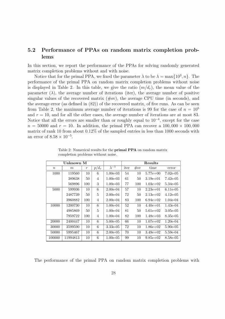
Notice that for the primal PPA, we fixed the parameter λ to be λ = max103, n. Theperformance of the primal PPA on random matrix completion problems without noiseis displayed in Table 2. In this table, we give the ratio (m/dr), the mean value of theparameter (λ), the average number of iterations (iter), the average number of positivesingular values of the recovered matrix (#sv), the average CPU time (in seconds), andthe average error (as defined in (82)) of the recovered matrix, of five runs. As can be seenfrom Table 2, the maximum average number of iterations is 99 for the case of n = 105

and r = 10, and for all the other cases, the average number of iterations are at most 83.Notice that all the errors are smaller than or roughly equal to 10−4, except for the casen = 50000 and r = 10. In addition, the primal PPA can recover a 100, 000 × 100, 000matrix of rank 10 from about 0.12% of the sampled entries in less than 1000 seconds withan error of 8.58× 10−5.

Table 2: Numerical results for the primal PPA on random matrixcompletion problems without noise.

Unknown M Resultsn m r p/dr λ−1 iter #sv time error1000 119560 10 6 1.00e-03 54 10 5.77e+00 7.02e-05

389638 50 4 1.00e-03 61 50 3.19e+01 7.42e-05569896 100 3 1.00e-03 77 100 1.03e+02 5.34e-05

5000 599936 10 6 2.00e-04 57 10 2.23e+01 6.11e-052487739 50 5 2.00e-04 72 50 2.13e+02 4.12e-053960882 100 4 2.00e-04 83 100 6.94e+02 1.04e-04

10000 1200730 10 6 1.00e-04 52 10 4.40e+01 1.43e-044985869 50 5 1.00e-04 81 50 5.61e+02 3.05e-057959722 100 4 1.00e-04 82 100 1.48e+03 8.35e-05

20000 2400447 10 6 5.00e-05 66 10 1.07e+02 1.20e-0430000 3599590 10 6 3.33e-05 72 10 1.86e+02 5.90e-0550000 5995467 10 6 2.00e-05 70 10 3.49e+02 5.59e-04

100000 11994813 10 6 1.00e-05 99 10 9.85e+02 8.58e-05

The performance of the primal PPA on random matrix completion problems with

28

noise is displayed in Table 3. We report the same results as in Table 2. As can be seenfrom Table 3, the primal PPA takes at most 67 iterations on the average to recover theunknown matrices. More importantly, the relative errors are all smaller than 7.94× 10−2,which is smaller than the given noise level of κ = 0.1.

Table 3: Numerical results for the primal PPA on random matrixcompletion problems with noise. The noise factor κ is set to 0.1.

Unknown M Resultsn /κ m r p/dr λ−1 iter #sv time error

1000 /0.10 119560 10 6 1.00e-03 38 10 5.10e+00 5.62e-02389638 50 4 1.00e-03 47 51 3.16e+01 7.74e-02569896 100 3 1.00e-03 45 100 5.80e+01 7.94e-02

5000 /0.10 599936 10 6 2.00e-04 45 10 2.38e+01 5.02e-022487739 50 5 2.00e-04 53 50 2.23e+02 5.93e-023960882 100 4 2.00e-04 47 100 4.93e+02 7.72e-02

10000 /0.10 1200730 10 6 1.00e-04 45 10 5.59e+01 4.89e-024985869 50 5 1.00e-04 36 50 3.62e+02 5.84e-027959722 100 4 1.00e-04 57 100 1.24e+03 6.82e-02

20000 /0.10 2400447 10 6 5.00e-05 47 10 9.32e+01 5.60e-0230000 /0.10 3599590 10 6 3.33e-05 53 10 1.69e+02 4.80e-0250000 /0.10 5995467 10 6 2.00e-05 58 10 3.33e+02 5.24e-02

100000 /0.10 11994813 10 6 1.00e-05 67 10 7.53e+02 5.42e-02

In Table 4 and Table 5, we report the performance of the dual PPA on random matrixcompletion problems without and with noise, respectively. Note that for the dual PPA,we fixed λ to be λ = 104/‖A∗(b)‖2. As shown in the tables, we can see that the dual PPAworks well with relatively small values of λ.

Comparing the performance of the primal PPA and the dual PPA on random matrixcompletion problems without/with noise, we observe that the dual PPA outperforms theprimal PPA2. For the case n = 105 and r = 10 without noise, the dual PPA solvesthe problem in 519 seconds whereas the primal PPA takes 985 seconds. There are twopossible reasons to explain this difference. First, the inner sub-problems of the dual PPAare solved by an APG method, while those of the primal PPA are solved by a gradientprojection method. Second, the former works well with relatively small values of λ, whilethe latter requires larger values of λ. However, a larger value of λ often leads to a slowerrate of convergence for the outer iteration in the PPA.

2Here our conclusion is based on using the gradient-type methods to solve the corresponding sub-problems.

29

Table 4: Numerical results for the dual PPA on random matrixcompletion problems without noise.

Unknown M Resultsn m r p/dr λ−1 iter #sv time error1000 119560 10 6 1.44e-02 35 10 3.90e+00 1.05e-04

389638 50 4 5.37e-02 51 50 2.95e+01 6.21e-05569896 100 3 8.66e-02 56 100 7.78e+01 2.41e-05

5000 599936 10 6 1.38e-02 42 10 1.71e+01 7.34e-052487739 50 5 6.08e-02 50 50 1.47e+02 6.50e-053960882 100 4 1.02e-01 56 100 4.32e+02 9.68e-05

10000 1200730 10 6 1.37e-02 40 10 2.96e+01 1.40e-044985869 50 5 5.93e-02 51 50 3.19e+02 6.54e-057959722 100 4 9.88e-02 56 100 9.05e+02 1.04e-04

20000 2400447 10 6 1.35e-02 45 10 6.72e+01 1.50e-0430000 3599590 10 6 1.35e-02 54 10 1.21e+02 1.41e-0450000 5995467 10 6 1.34e-02 58 10 2.46e+02 4.83e-05

100000 11994813 10 6 1.34e-02 55 10 5.19e+02 1.04e-04

Table 5: Numerical results for the dual PPA on random matrixcompletion problems with noise. The noise factor is set to 0.1.

Unknown M Resultsn m r p/dr λ−1 iter #sv time error

1000 /0.10 119560 10 6 1.44e-02 29 10 3.95e+00 4.49e-02389638 50 4 5.37e-02 31 50 1.52e+01 5.49e-02569896 100 3 8.67e-02 39 100 4.36e+01 6.39e-02

5000 /0.10 599936 10 6 1.38e-02 39 10 2.20e+01 4.51e-022487739 50 5 6.08e-02 39 50 1.09e+02 4.96e-023960882 100 4 1.02e-01 41 100 2.71e+02 5.67e-02

10000 /0.10 1200730 10 6 1.37e-02 44 10 4.73e+01 4.53e-024985869 50 5 5.93e-02 39 50 2.26e+02 4.99e-027959722 100 4 9.89e-02 47 100 6.92e+02 5.73e-02

20000 /0.10 2400447 10 6 1.35e-02 44 10 9.65e+01 4.52e-0230000 /0.10 3599590 10 6 1.35e-02 45 10 1.45e+02 4.53e-0250000 /0.10 5995467 10 6 1.34e-02 47 10 2.70e+02 4.53e-02

100000 /0.10 11994813 10 6 1.34e-02 43 10 5.42e+02 4.53e-02

Remark 5.1. Here we do not report the numerical results for the primal-dual PPA-I andPPA-II for the sake of saving some space. Indeed, in our experiments, we observe that

30

the performance of the primal-dual PPA-I is similar to that of the primal PPA, and theperformance of the primal-dual PPA-II is similar to that of the dual PPA.

5.3 Performance of the dual PPA on real matrix completionproblems

Now we consider the well-known matrix completion problem in the Netflix Prize Contest[37]. Three data sets are provided in the Contest.

1. training set: consists of about 100 million ratings from 480189 randomly chosenusers on 17770 movie titles. The ratings are integers on a scale from 1 to 5.

2. qualifying set: contains over 2.8 million user/movie pairs but with the ratingswithheld. The qualifying set is further randomly divided into two disjoint subsetscalled quiz and test subsets.

3. probe set: this is a subset of the training set consisting of about 1.4 millionuser/movie pairs with known ratings. This subset is constructed to have similarproperties as the qualifying set.

For convenience, we assume that the users are enumerated from 1 to 480189, and themovies are enumerated from 1 to 17770. We define

Ωt =(i, j) : user i has rated movie j in the training set

,

Ωq =(i, j) : user i has rated movie j in the qualifying set

,

Ωp =(i, j) : user i has rated movie j in the probe set

.

The Netflix Prize Contest solicits algorithms that can make predictions for all thewithheld ratings for the user/movie pairs in the qualifying set. The quality of thepredictions is measured by the root mean squared error:

RMSE =

1

|Ωq|∑

(k,j)∈Ωq

(xpredkj − xtrue

kj )2

1/2

,

where xpredkj , xtrue

kj are the predicted and actual ratings for the k-th user on the j-th movie.For any predictions submitted to the Contest, the RMSE for the quiz subset will bereported publicly on [37] whereas the RMSE for the test subset is withheld but willbe employed for the purpose of selecting the winner in the Contest. At the start of theContest, the RMSE of Netflix’s proprietary Cinematch algorithm on the quiz and test

subsets, based on the training data set alone, were 0.9514 and 0.9525, respectively. TheRMSE obtained by the Cinematch algorithm on the probe set is 0.9474.

31

Due to memory constraint, in our numerical experiment, we divide the training set

and probe set respectively into 5 disjoint subsets according to the users’ id as follows:

training-k =(i, j) ∈ Ωt\Ωp : (k − 1)100, 000 < i ≤ (k + 1)100, 000

,

probe-k =(i, j) ∈ Ωp : (k − 1)100, 000 < i ≤ (k + 1)100, 000

, k = 1, . . . , 5.

Note that we removed the data in the probe set from the training set in the experi-ments.

We apply the dual PPA to (4) for all the 5 subsets to predict the ratings of all theusers on all the movies. As the noise level δ for these problems are not known, weestimate δ dynamically from (outer) iteration to iteration. That is, for the k-th outeriteration in the dual PPA, we set δ = 0.5‖b − A(Xk)‖. In addition, as the optimalsolutions of these problems are not necessarily low-rank, we truncate the rank of Xj+1 =PL−1 [Y j − L−1∇h(Y j)] in the APG algorithm (78) to 10 in each iteration of the APGalgorithm. We have tested truncating the rank to 50, but the results were slightly worse.

For each of the subsets training-k, we compute the RMSE for the correspondingprobe subsets probe-k. Table 6 shows the results we obtained. We should note thatin our experiment, we do not preprocess the data sets via any statistical means, exceptto center the partially observed matrix Mk corresponding to training-k such that themodified matrix Mk has all its rows and columns each having zero sum. That is,

Mkij = Mk

ij − di − fj, ∀ i, j

and di, fj are determined so that∑

j Mkij = 0 and

∑i M

kij = 0 for all i and j.

Table 6: Numerical results for the dual PPA on matrix completionproblems arising from Netflix Contest. The number of movies is17770.

Unknown M Results

n m λ−1 iter #sv timetrainingRMSE

probeRMSE

training-1 100000 2.08e+07 2.92e+00 35 10 3.9e+02 0.8148 0.9309

training-2 100000 2.08e+07 2.93e+00 35 10 4.0e+02 0.8126 0.9292

training-3 100000 2.09e+07 2.93e+00 35 10 4.0e+02 0.8131 0.9278

training-4 100000 2.07e+07 2.94e+00 35 10 3.9e+02 0.8152 0.9331

training-5 80189 1.66e+07 2.64e+00 35 10 2.9e+02 0.8136 0.9366

training\probe 160378 9.98e+07 1.9e+03 0.8139 0.9313

32

As we can observe from Table 6, the training set (with probe set removed) RMSEis much lower than the probe set RMSE, and this reflects that the dual PPA on (4) overtrains the data. Despite that, the probe set RMSE of 0.9313 we obtained is betterthan that obtained by Netflix’s Cinematch algorithm. The computed RMSE for the quizsubset is 0.9416.

6 Conclusions and discussions

In this paper, we have proposed implementable proximal point algorithms in the primal,dual and primal-dual forms for solving the nuclear norm minimization problem with linearequality and second order cone constraints, and presented comprehensive convergence re-sults. These algorithms are efficient and competitive to state-of-the-art alternatives whenthe inner sub-problems of these algorithms are solved by either the gradient projectionmethod or the accelerated proximal point method.

Before closing this paper, we would like to discuss future research directions related tothis work. Firstly, our algorithms achieve linear rate of convergence under the conditionthat T −1

f or T −1g or T −1

l is Lipschitz continuous at the origin. It is then interesting toknow whether one can characterize these conditions as in [47]. Secondly, it would be worthexploring the performance of these algorithms in which the inner sub-problems are solvedby second-order methods such as semismooth Newton and smoothing Newton methods,where applicable. Finally, we plan to study how the general framework presented in thispaper can help solve more general nuclear norm optimization problems.

References

[1] Alfakih, A.Y., Khandani, A. and Wolkowicz, H., Solving Euclidean distance matrixcompletion problems via semidefinite programming, Comp. Optim. Appl. 12 (1999),13–30.

[2] Ames, B.P.W. and Vavasis, S.A., Nuclear norm minimization for the planted cliqueand biclique problems, preprint, 2009.

[3] Barvinok, A., Problems of distance geometry and convex properties of quadratic maps,Discrete Computational Geometry, 13 (1995), 189–202.

[4] Beck, A. and Teboulle, M., A fast iterative shrinkage-thresholding algorithm for linearinverse problems, SIAM J. Imaging Sciences 1 (2009), 183–202.

[5] Bertsekas, D.P., On the Goldstein-Levitin-Polyak gradient projection method, IEEETrans. Automatic Control 21 (1976), 174–184.

[6] Bertsekas, D.P., Nonlinear Programming, 2nd edition, Athena Scientific, Belmont,1999.

33

[7] Burer, S. and Monteiro, R.D.C., A nonlinear programming algorithm for solvingsemidefinite programs via low-rank factorization, Math. Program. 95 (2003), 329–357.

[8] Burer, S. and Monteiro, R.D.C., Local minima and convergence in low-rank semidef-inite programs, Math. Program. 103 (2005), 427–444.

[9] Cai, J.-F., Candes, E.J. and Shen, Z.W., A singular value thresholding algorithm formatrix completion, preprint available at http://arxiv.org/abs/0810.3286.

[10] Candes, E.J., Compressive sampling, In International Congress of Mathematicians.Vol. III, Eur. Math. Soc., Zourich, 1433–1452, 2006.

[11] Candes, E.J. and Becker, S., Singular value thresholding – codes for the SVT algo-rithm to minimize the nuclear norm of a matrix, subject to linear constraints, April2009. Available at http://svt.caltech.edu/code.html.

[12] Candes, E.J. and Tao, T., Nearly optimal signal recovery from random projections:Universal encoding strategies, IEEE Trans. Info. Theory 52 (2006), 5406–5425.

[13] Candes, E.J. and Recht, B., Exact matrix completion via convex optimization,preprint, 2008.

[14] Donoho, D., Compressed sensing, IEEE Trans. Info. Theory 52 (2006), 1289–1306.

[15] Faraut, U. and Koranyi, A., Analysis on Symmetric Cones, Oxford MathematicalMonographs, Oxford University Press, New York, 1994.

[16] Fazel, M., Matrix rank minimization with applications, Ph.D. thesis, Stanford Uni-versity, 2002.

[17] Fazel, M., Hindi, H. and Boyd, S., A rank minimization heuristic with applicationto minimum order system approximation, In Proceedings of the American ControlConference, 2001.

[18] Fazel, M., Hindi, H. and Boyd, S., Log-det heuristic for matrix rank minimizationwith applications to Hankel and Euclidean distance matrices, In Proceedings of theAmerican Control Conference, 2003.

[19] Gafni, E.H. and Bertsekas, D.P., Two-metric projection methods for constrained op-timization, SIAM J. Control Optim. 22 (1984), 936–964.

[20] Ghaoui, L.E. and Gahinet, P., Rank minimiztion under LMI constraints: A frame-work for output feedback problems, In Proceedings of the European Control Confer-ence, 1993.

34

[21] Goldstein, A.A., Convex programming in Hilbert space, Bull. Amer. Math. Soc. 70(1964), 709–710.

[22] Hiriart-Urruty, J.-B. and Lemarechal, C., Convex Analysis and Minimization Algo-rithms, Vols. 1 and 2, Springer-Verlag, Berlin, Heidelberg, New York, 1993.

[23] Lan, G., Lu, Z. and Monteiro, R.D.C., Primal-dual first-order methods with O(1/ε)iteration-complexity for cone programming, to appear in Mathematical Programming.

[24] Larsen, R.M., PROPACK–Software for large and sparse SVD calculations, Availablefrom http://sun.stanfor.edu/∼rmunk/PROPACK/.

[25] Lemarechal, C. and Sagastizabal, C., Practical aspects of the Moreau-Yosida regular-ization I: theoretical preliminaries, SIAM J. Optim. 7 (1997), 367–385.

[26] Levitin, E.S. and Polyak, B.T., Constrained minimization problems, USSR Compu-tational Mathematics and Mathematical Physics 6 (1966), 1–50.

[27] Linial, N., London, E. and Rabinovich, Y., The geometry of graphs and some of itsalgorithmic applications, Combinatorica 15 (1995), 215–245.

[28] Liu, Z. and Vandenberghe, L., Interior-point method for nuclear norm approximationwith application to system identification, preprint, 2008.

[29] Lu, F., Keles, S., Wright, S.J. and Wahba, G., A framework for kernel regulariza-tion with application to protein clustering, Proceedings of the National Academy ofSciences, 102 (2005), 12332–12337.

[30] Ma, S.Q., Goldfarb, D. and Chen, L.F., Fixed point and Bregman iterative methodsfor matrix rank minimization, preprint, 2008.

[31] Moreau, J.J., Proximite et dualite dans un espace hilbertien, Bulletin de la SocieteMathematique de France, 93 (1965), 273–299.

[32] Nemirovski, A., Prox-method with rate of convergence O(1/t) for variational inequali-ties with Lipschitz continuous monotone operators and smooth convex-concave saddlepoint problems, SIAM J. Optim. 15 (2005), 229–251.

[33] Nesterov, Y.E., A method for unconstrained convex minimization problem with therate of convergence O(1/k2), Doklady AN SSSR, 269 (1983), 543–547.

[34] Nesterov, Y.E., Introductory Lectures on Convex Optimization: A Basic Course,Kluwer Academic Publishers, Dordrecht, The Netherlands, 2004.

[35] Nesterov, Y.E., Smooth minimization of nonsmooth functions, Math. Program. 103(2005), 127–152.

35

[36] Nesterov, Y.E., Gradient methods for minimizing composite objective function, Re-port, CORE, Catholic University of Louvain, Louvain-la-Neuve, Belgium, September,2007.

[37] Netflix Prize: http://www.netflixprize.com/.

[38] Recht, B., Fazel, M. and Parrilo, P.A., Guaranteed minimum-rank solutionsof linear matrix equations via nuclear norm minimization, preprint available athttp://arxiv.org/abs/0706.4138.

[39] Rockafellar, R.T., Convex Analysis, Princeton University Press, Princeton, 1970.

[40] Rockafellar, R.T., Monotone operators and the proximal point algorithm, SIAM J.Control Optim. 14 (1976), 877–898.

[41] Rockafellar, R.T., Augmented Lagrangians and applications of the proximal pointalgorithm in convex programming, Math. Oper. Res. 1 (1976), 97–116.

[42] Sturm, J.F., Using SeDuMi 1.02, a Matlab toolbox for optimization over symmetriccones, Optim. Methods Softw. 11-12 (1999), 625–653.

[43] Toh, K.C. and Yun, S.W., An accelerated proximal gradient algorithm for nuclearnorm regularized least squares problems, preprint, National University of Singapore,2009.

[44] Tseng, P., On accelerated proximal gradient method for convex-concave optimization,preprint, University of Washington, 2008.

[45] Tutuncu, R.H., Toh, K.C. and Todd, M.J., Solving semidefinite-quadratic-linear pro-grams using SDPT3, Math. Program. 95 (2003), 189–217.

[46] Yosida, K., Functional Analysis, Springer Verlag, Berlin, 1964.

[47] Zhao, X.Y., Sun, D.F. and Toh, K.C., A Newton-CG augmented Lagrangian methodfor semidefinite programming, preprint, National University of Singapore, March2008.

36