An Illustrated Guide to Low-cost, Side Scan Sonar Habitat Mapping

An Illustrated Guide to Low-cost, Side Scan Sonar Habitat Mapping

Adam J. Kaeser, Ph.D. Aquatic Ecologist U.S. Fish and Wildlife Service 1601 Balboa Avenue Panama City, Florida 32405 [email protected] (850) 769-0552, ext. 244

Thom L. Litts, MSc GIS GIS Specialist Georgia Department of Natural Resources Social Circle, Georgia [email protected] (706) 557-3236

by Adam J. Kaeser and Thom L. Litts March 2013

The Authors

1

mailto:[email protected]

Preface

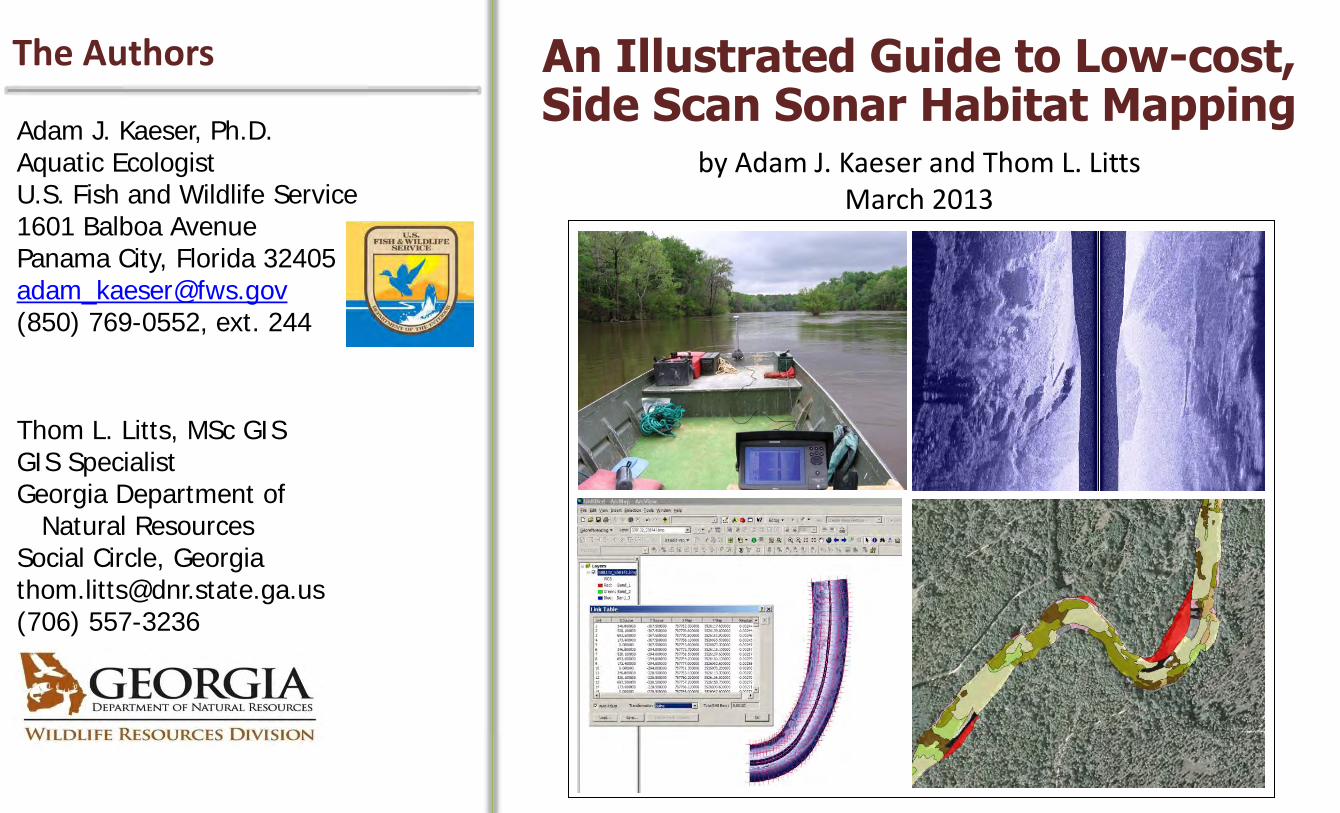
This guidebook represents the fully annotated version of a Continuing Education workshop prepared by Kaeser and Litts to train natural resource professionals interested in low-cost, side scan sonar mapping in navigable, aquatic systems. This workshop was first presented at an early 2008 meeting of the Southern Division of the American Fisheries Society in Wheeling, West Virginia, and has since been presented over a dozen times nationwide. Over this time the program has been substantially revised and improved. In the spirit of widespread access and outreach, we have prepared this guidebook to provide the information electronically to anyone interested in the pursuit of sonar habitat mapping. The program is divided into several sessions that successively build upon one another with the ultimate goal of establishing a foundation for the method we call low-cost sonar habitat mapping. This foundation includes understanding, planning, and executing a sonar mapping survey, geoprocessing the collected sonar data, preparing classified habitat layers by visual interpretation of transformed sonar imagery, evaluating elements of map accuracy, and exploring applications. The live workshop incorporates a virtual demonstration of the geoprocessing approach and tools developed by Litts for creation of the sonar image map layers. The technical details of this process are tackled with the aid of the Sonar Imagery Geoprocessing Workbook and a demonstration data set that accompanies this Guide.

Sonar Mapping Workshop

TXAFS- San Marcos, TX, February 2011 2

SDAFS Reservoir Committee

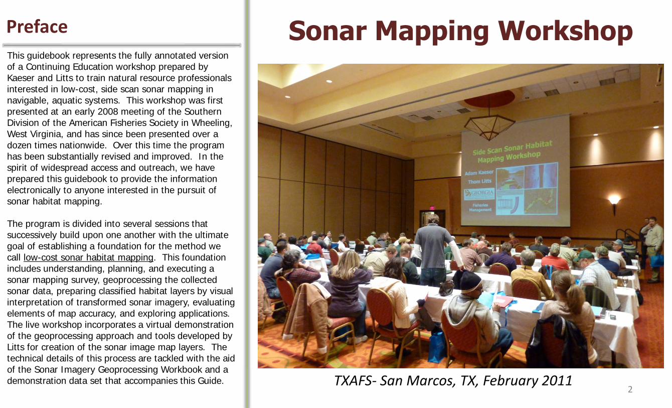
We gratefully acknowledge support for this work provided by:

University of Georgia

3

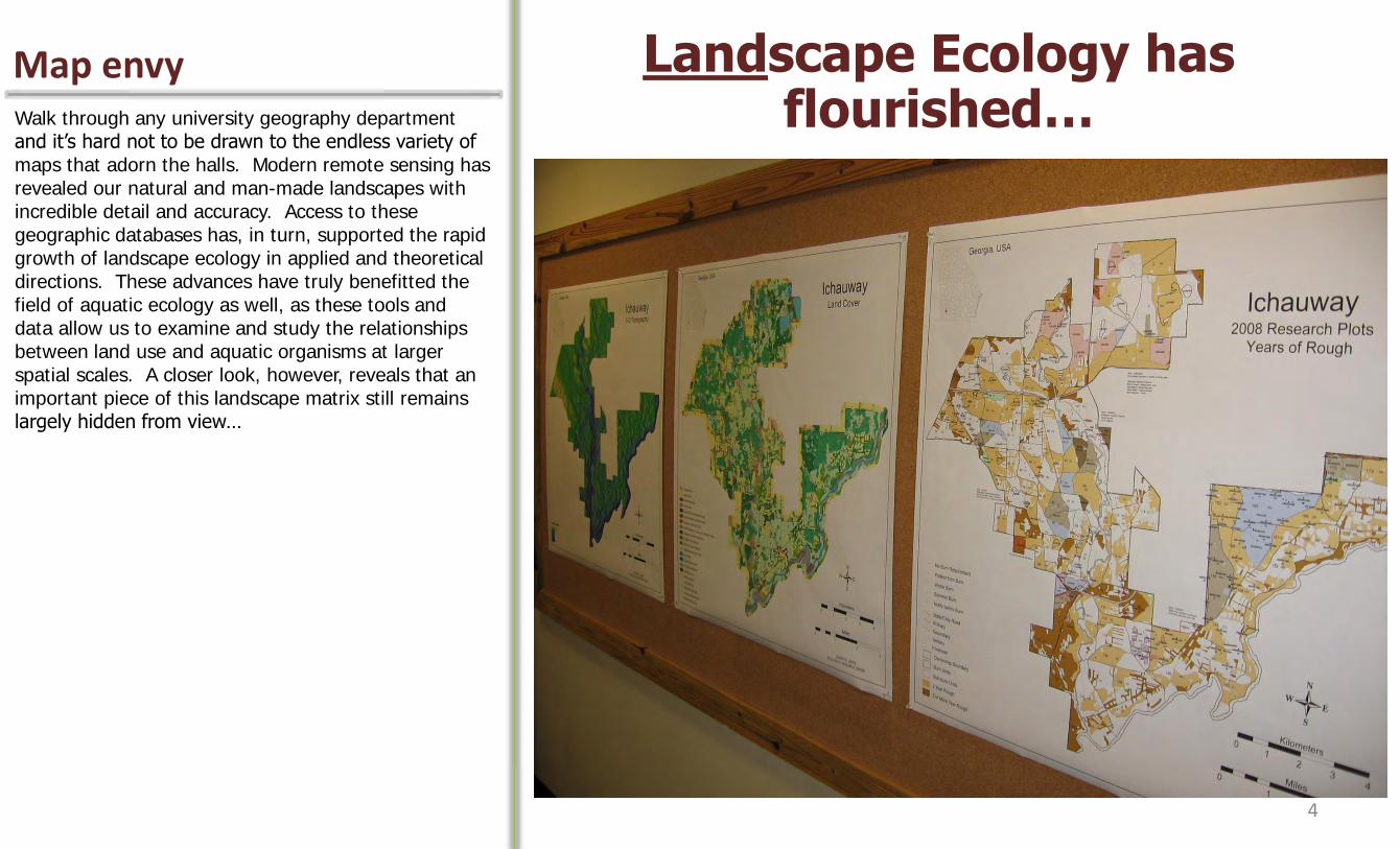
Landscape Ecology has flourished… Walk through any university geography department

and it’s hard not to be drawn to the endless variety of maps that adorn the halls. Modern remote sensing has revealed our natural and man-made landscapes with incredible detail and accuracy. Access to these geographic databases has, in turn, supported the rapid growth of landscape ecology in applied and theoretical directions. These advances have truly benefitted the field of aquatic ecology as well, as these tools and data allow us to examine and study the relationships between land use and aquatic organisms at larger spatial scales. A closer look, however, reveals that an important piece of this landscape matrix still remains largely hidden from view…

Map envy

4

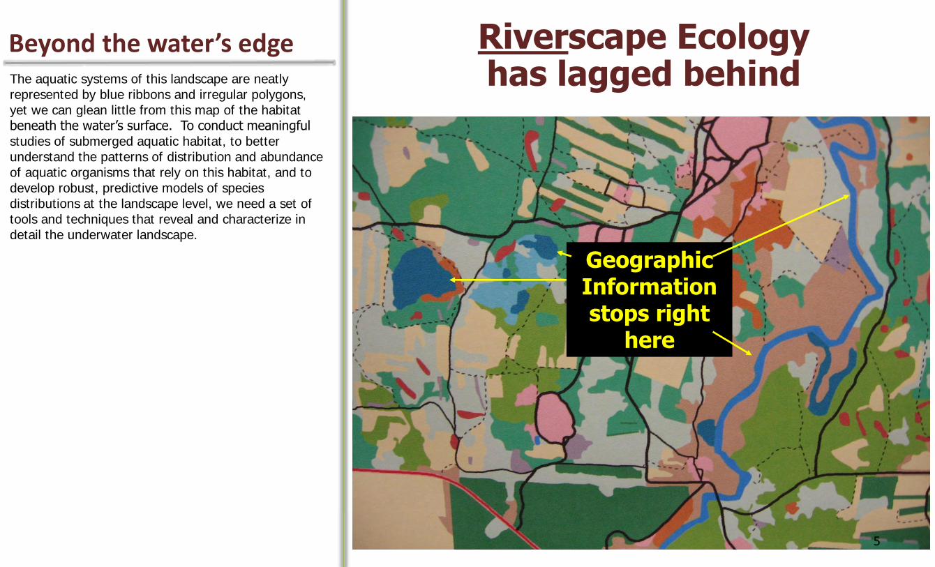
The aquatic systems of this landscape are neatly represented by blue ribbons and irregular polygons, yet we can glean little from this map of the habitat beneath the water’s surface. To conduct meaningful studies of submerged aquatic habitat, to better understand the patterns of distribution and abundance of aquatic organisms that rely on this habitat, and to develop robust, predictive models of species distributions at the landscape level, we need a set of tools and techniques that reveal and characterize in detail the underwater landscape.

Beyond the water’s edge Riverscape Ecology has lagged behind

Geographic Information stops right

here

5

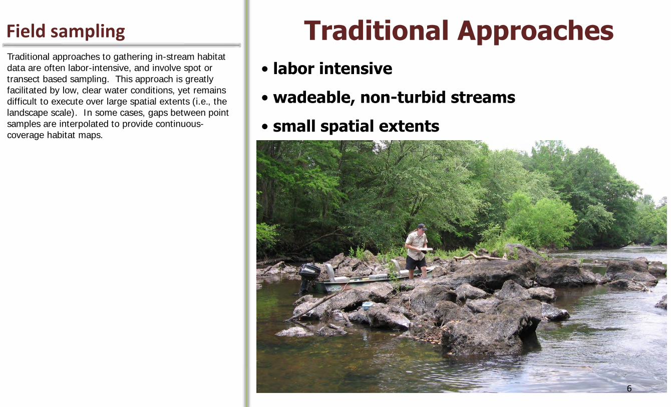
Field sampling Traditional Approaches

• labor intensive

• wadeable, non-turbid streams

• small spatial extents

Traditional approaches to gathering in-stream habitat data are often labor-intensive, and involve spot or transect based sampling. This approach is greatly facilitated by low, clear water conditions, yet remains difficult to execute over large spatial extents (i.e., the landscape scale). In some cases, gaps between point samples are interpolated to provide continuous-coverage habitat maps.

6

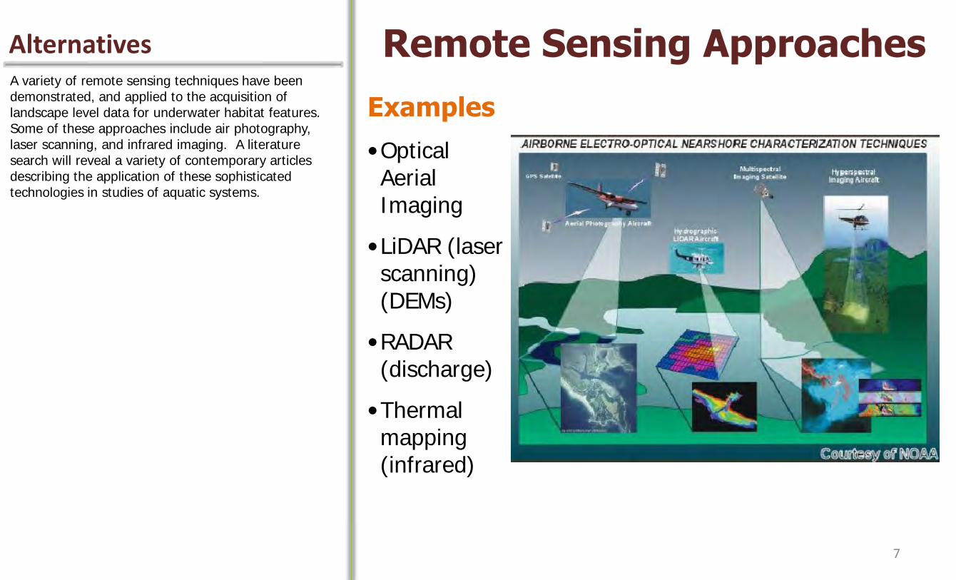
Alternatives Remote Sensing Approaches A variety of remote sensing techniques have been demonstrated, and applied to the acquisition of landscape level data for underwater habitat features. Some of these approaches include air photography, laser scanning, and infrared imaging. A literature search will reveal a variety of contemporary articles describing the application of these sophisticated technologies in studies of aquatic systems.

Examples

•Optical Aerial Imaging

•LiDAR (laser scanning) (DEMs)

•RADAR (discharge)

•Thermal mapping (infrared)

7

Alternatives Remote Sensing Approaches These hi-tech approaches are, however, challenged by one or more financial, logistical, or physical limitations; we suspect these factors will continue to preclude or inhibit the widespread adoption of these methods for mapping aquatic habitat. As illustrated here, many approaches demand the airborne deployment of a sensor system- a non-trivial expense in the budget of any mapping project. The systems are also quite expensive, and require technical expertise and specialized software for operation and processing of acquired data. Even if associated expenses and technical expertise are covered, a variety of physical limitations such as depth, turbidity, and overhead canopy cover prevent the acquisition of data using airborne systems from many navigable waterways, especially those common to the Southeast Coastal Plain where we conduct our work.

Limitations

Financial-Logistical

Sensor systems- $$$

Airborne surveys- $$$

Technical specialists,

software required- $$$

Physical

Depth, Turbidity, Overhead (Canopy) Cover

8

“Sound” imaging in nature Nature Invented SONAR Long ago nature invented a means for visualizing terrestrial and aquatic environments using high frequency sound waves. SONAR (sound and navigation ranging) overcomes the visual limitations imposed by nightfall or turbidity.

9

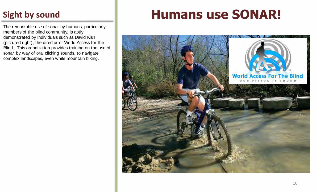
Sight by sound Humans use SONAR! The remarkable use of sonar by humans, particularly members of the blind community, is aptly demonstrated by individuals such as David Kish (pictured right), the director of World Access for the Blind. This organization provides training on the use of sonar, by way of oral clicking sounds, to navigate complex landscapes, even while mountain biking.

10

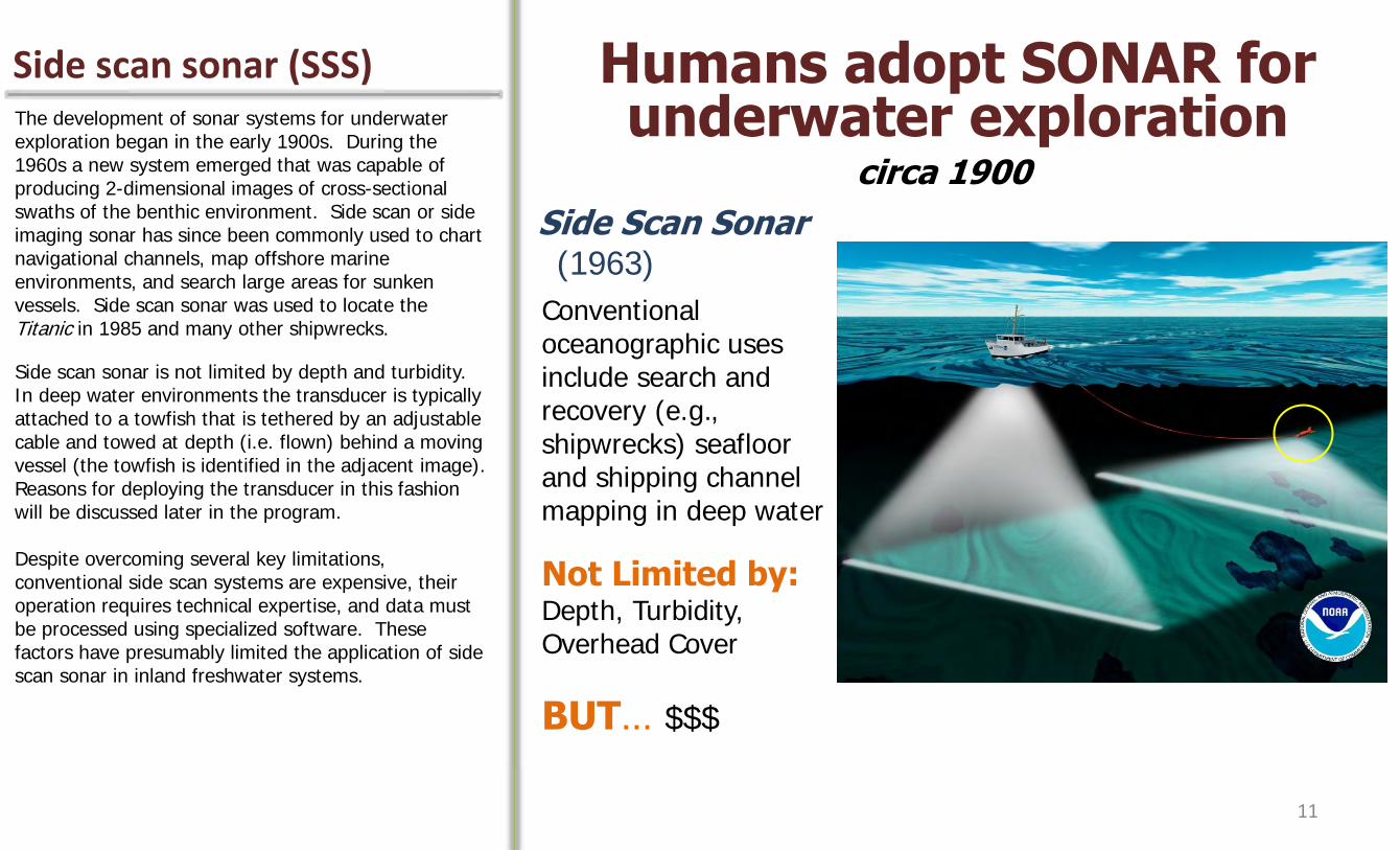
Side scan sonar (SSS) Humans adopt SONAR for underwater exploration The development of sonar systems for underwater

exploration began in the early 1900s. During the 1960s a new system emerged that was capable of producing 2-dimensional images of cross-sectional swaths of the benthic environment. Side scan or side imaging sonar has since been commonly used to chart navigational channels, map offshore marine environments, and search large areas for sunken vessels. Side scan sonar was used to locate the Titanic in 1985 and many other shipwrecks.

Side scan sonar is not limited by depth and turbidity. In deep water environments the transducer is typically attached to a towfish that is tethered by an adjustable cable and towed at depth (i.e. flown) behind a moving vessel (the towfish is identified in the adjacent image). Reasons for deploying the transducer in this fashion will be discussed later in the program. Despite overcoming several key limitations, conventional side scan systems are expensive, their operation requires technical expertise, and data must be processed using specialized software. These factors have presumably limited the application of side scan sonar in inland freshwater systems.

circa 1900

Side Scan Sonar (1963)

Conventional oceanographic uses include search and recovery (e.g., shipwrecks) seafloor and shipping channel mapping in deep water

Not Limited by: Depth, Turbidity, Overhead Cover

BUT… $$$

11

Recreational SSS Humminbird® Side Imaging System In 2005 the Humminbird® Company, based in Eufaula

Alabama, introduced the first recreational grade side scan sonar system, a product that has dramatically changed the sonar landscape, to say the least. The Humminbird® Side Imaging (HSI) system offers two primary advantages over conventional systems- high quality imagery at a very low price, and a small adjustable transducer that can be deployed on a small watercraft. The affordability of the hardware is a major reason why we have dubbed this enterprise “low-cost” sonar habitat mapping.

Introduced 2005

2 Major Advances-

1) High quality imagery at low price

2) Small adjustable transducer

~$2,000-$2,700

The cost for a new Side Imaging system ranges from $2000-2700. Humminbird® primarily markets the system to professional and serious amateur fishermen, although several other user groups, like divers, have also embraced the product. *Kaeser and Litts are NOT representatives of the Humminbird® Company, and have not received any funding or support from Humminbird® for their work. 12

Recreational SSS Lowrance equivalent- StructureScan For several years, the Humminbird® Side Imaging

system was the only recreational grade side scan system, but in 2009 Lowrance released their version of SSS called StructureScan. This is a modular system, and the StructureScan component must be integrated with other Lowrance sonar modules. Since 2006 we have worked exclusively with the Humminbird® Side Imaging system, and cannot offer much advice on the operation of the Lowrance StructureScan. We have fielded several inquiries regarding whether our geoprocessing methodology can be adapted for StructureScan imagery. At the time of writing this remains an untested possibility, although in theory the methodology should be transferable. For an up-to-date synopsis of this issue, please contact the authors.

Introduced Summer 2009

13

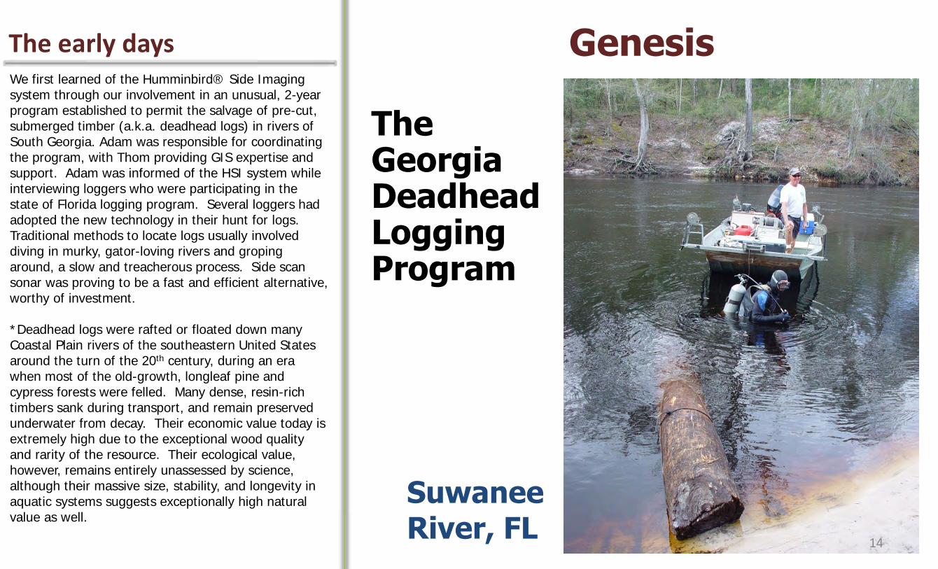
The early days Genesis We first learned of the Humminbird® Side Imaging system through our involvement in an unusual, 2-year program established to permit the salvage of pre-cut, submerged timber (a.k.a. deadhead logs) in rivers of South Georgia. Adam was responsible for coordinating the program, with Thom providing GIS expertise and support. Adam was informed of the HSI system while interviewing loggers who were participating in the state of Florida logging program. Several loggers had adopted the new technology in their hunt for logs. Traditional methods to locate logs usually involved diving in murky, gator-loving rivers and groping around, a slow and treacherous process. Side scan sonar was proving to be a fast and efficient alternative, worthy of investment. *Deadhead logs were rafted or floated down many Coastal Plain rivers of the southeastern United States around the turn of the 20th century, during an era when most of the old-growth, longleaf pine and cypress forests were felled. Many dense, resin-rich timbers sank during transport, and remain preserved underwater from decay. Their economic value today is extremely high due to the exceptional wood quality and rarity of the resource. Their ecological value, however, remains entirely unassessed by science, although their massive size, stability, and longevity in aquatic systems suggests exceptionally high natural value as well.

The Georgia Deadhead Logging Program

Suwanee River, FL

14

Hunting deadheads Deadhead Logs Side scan sonar permitted loggers to quickly survey long reaches of river in search of deadheads. The adjacent raw sonar image was captured in a slough of a large, Coastal Plain river. Along the left side of the boat, a nice cache of deadhead logs are seen resting on the sandy bottom. The long, straight, and uniformly cylindrical shape of these objects are tell-tale characteristics of deadhead logs. In some cases, only the sonar shadow being cast by the log is visible. Several logs appear to be partially embedded in sediment. *A log cache represents real value to a logging crew in terms of focusing salvage efforts. Given that a each deadhead log might fetch between $200-400 when sold to a mill, this cache of logs would be welcome discovery.

15

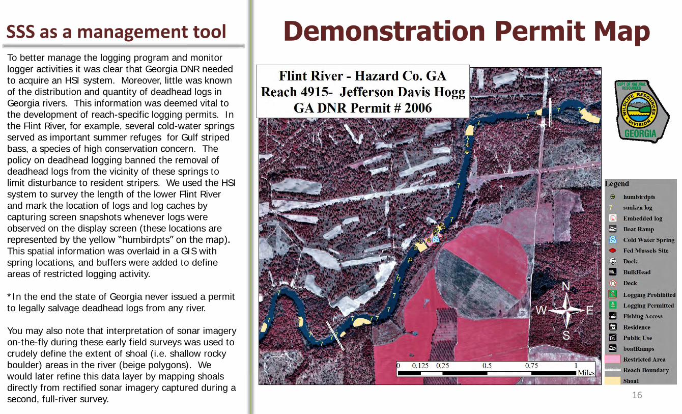
SSS as a management tool Demonstration Permit Map To better manage the logging program and monitor logger activities it was clear that Georgia DNR needed to acquire an HSI system. Moreover, little was known of the distribution and quantity of deadhead logs in Georgia rivers. This information was deemed vital to the development of reach-specific logging permits. In the Flint River, for example, several cold-water springs served as important summer refuges for Gulf striped bass, a species of high conservation concern. The policy on deadhead logging banned the removal of deadhead logs from the vicinity of these springs to limit disturbance to resident stripers. We used the HSI system to survey the length of the lower Flint River and mark the location of logs and log caches by capturing screen snapshots whenever logs were observed on the display screen (these locations are represented by the yellow “humbirdpts” on the map). This spatial information was overlaid in a GIS with spring locations, and buffers were added to define areas of restricted logging activity. *In the end the state of Georgia never issued a permit to legally salvage deadhead logs from any river. You may also note that interpretation of sonar imagery on-the-fly during these early field surveys was used to crudely define the extent of shoal (i.e. shallow rocky boulder) areas in the river (beige polygons). We would later refine this data layer by mapping shoals directly from rectified sonar imagery captured during a second, full-river survey. 16

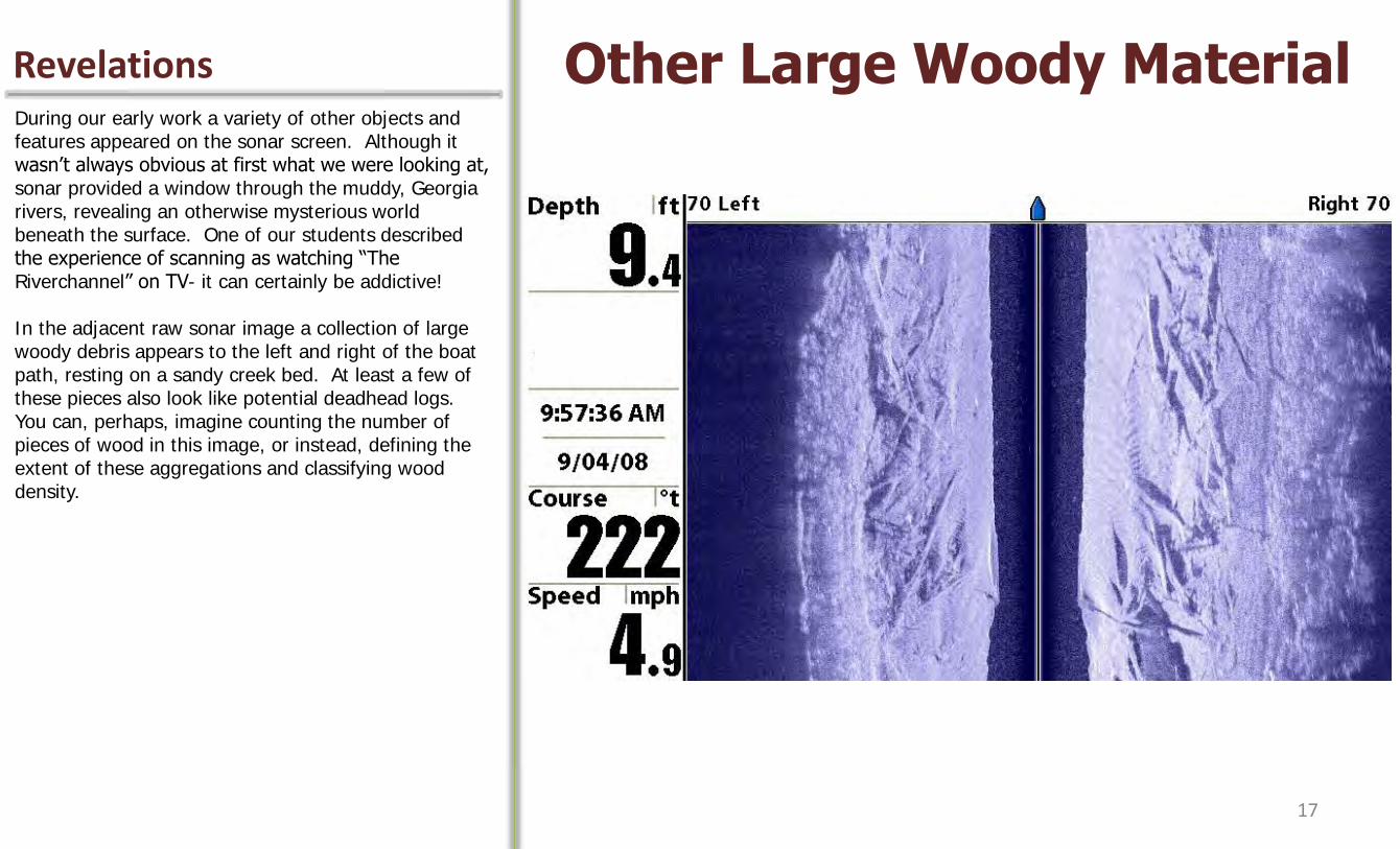
Revelations Other Large Woody Material During our early work a variety of other objects and features appeared on the sonar screen. Although it wasn’t always obvious at first what we were looking at, sonar provided a window through the muddy, Georgia rivers, revealing an otherwise mysterious world beneath the surface. One of our students described the experience of scanning as watching “The Riverchannel” on TV- it can certainly be addictive! In the adjacent raw sonar image a collection of large woody debris appears to the left and right of the boat path, resting on a sandy creek bed. At least a few of these pieces also look like potential deadhead logs. You can, perhaps, imagine counting the number of pieces of wood in this image, or instead, defining the extent of these aggregations and classifying wood density.

17

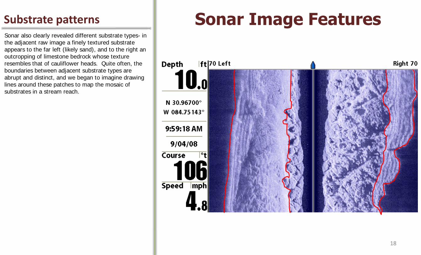
Substrate patterns Sonar Image Features Sonar also clearly revealed different substrate types- in the adjacent raw image a finely textured substrate appears to the far left (likely sand), and to the right an outcropping of limestone bedrock whose texture resembles that of cauliflower heads. Quite often, the boundaries between adjacent substrate types are abrupt and distinct, and we began to imagine drawing lines around these patches to map the mosaic of substrates in a stream reach.

18

We need a METHOD that integrates low-cost sonar imagery and GIS to map

underwater habitat!

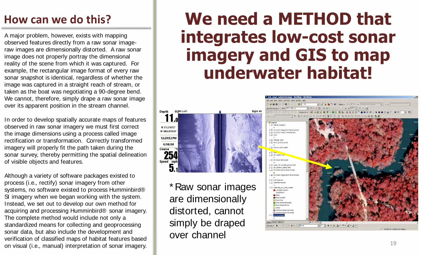
A major problem, however, exists with mapping observed features directly from a raw sonar image- raw images are dimensionally distorted. A raw sonar image does not properly portray the dimensional reality of the scene from which it was captured. For example, the rectangular image format of every raw sonar snapshot is identical, regardless of whether the image was captured in a straight reach of stream, or taken as the boat was negotiating a 90-degree bend. We cannot, therefore, simply drape a raw sonar image over its apparent position in the stream channel. In order to develop spatially accurate maps of features observed in raw sonar imagery we must first correct the image dimensions using a process called image rectification or transformation. Correctly transformed imagery will properly fit the path taken during the sonar survey, thereby permitting the spatial delineation of visible objects and features. Although a variety of software packages existed to process (i.e., rectify) sonar imagery from other systems, no software existed to process Humminbird® SI imagery when we began working with the system. Instead, we set out to develop our own method for acquiring and processing Humminbird® sonar imagery. The complete method would include not only a standardized means for collecting and geoprocessing sonar data, but also include the development and verification of classified maps of habitat features based on visual (i.e., manual) interpretation of sonar imagery.

*Raw sonar images are dimensionally distorted, cannot simply be draped over channel

How can we do this?

19

Guiding principles The “Ideal Method” would be: The “Ideal Method”, we reasoned, would satisfy five key principles: the method would be affordable (i.e., low-cost), fast yet accurate, applicable in a variety of aquatic settings, the training would be available and reasonable, and the necessary software or tools would be those readily available to professionals involved in both research and management of aquatic systems (e.g., ArcGIS).

• Affordable

• Fast, Efficient, and Accurate

• Applicable in diverse settings

• Training available and reasonable

• Software/tools accessible to researchers & managers

20

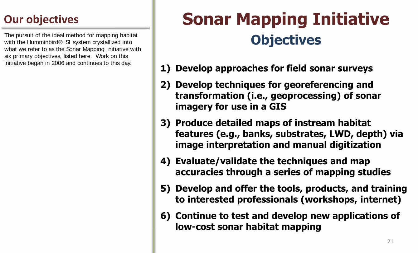
Our objectives Sonar Mapping Initiative The pursuit of the ideal method for mapping habitat with the Humminbird® SI system crystallized into what we refer to as the Sonar Mapping Initiative with six primary objectives, listed here. Work on this initiative began in 2006 and continues to this day.

Objectives

1) Develop approaches for field sonar surveys

2) Develop techniques for georeferencing and transformation (i.e., geoprocessing) of sonar imagery for use in a GIS

3) Produce detailed maps of instream habitat features (e.g., banks, substrates, LWD, depth) via image interpretation and manual digitization

4) Evaluate/validate the techniques and map accuracies through a series of mapping studies

5) Develop and offer the tools, products, and training to interested professionals (workshops, internet)

6) Continue to test and develop new applications of low-cost sonar habitat mapping

21

Training Workshop Objectives A major objective of the initiative was to develop and provide the training needed for successful application of low-cost sonar habitat mapping. This workshop was specifically designed to help people get started with side scan sonar. Although we attempt to address several relevant aspects of sonar habitat mapping, this workshop alone is only part of a continuous learning process that will hopefully lead to successful mapping project outcomes. We feel it is very important for those involved to work with the equipment in their systems of interest, and seek opportunities to improve skills in all facets of the mapping process, from boat handling and data capture, to image interpretation and the development and testing of new field applications. We fundamentally believe that freely available training materials are essential to the adoption and further development of this approach. This field will be expanded by those who find low-cost side scan sonar to be a useful, and perhaps indispensable tool to add to the natural resources toolkit.

• Provide an overview of side scan sonar technology and imagery

• Quick-start guide to complete method we call low-cost sonar habitat mapping

• Demonstrate the potential for mapping submerged features of aquatic environments using sonar image maps

22

Program sessions Workshop Format The workshop is divided into four consecutive sessions. The first session provides an introduction to side scan sonar basics. Given the importance of image interpretation to low-cost sonar habitat mapping, the following session tackles the fundamentals of this topic with a variety of example images from the field. Session I- Part A

Introduction to Side Scan Sonar

Session I- Part B

Image Interpretation

23

Program sessions Workshop Format Mission planning considerations, and steps taken during the execution of a sonar survey are topics covered in the second full session of the workshop.

Session II- Part A

Mission Planning

Session II- Part B

Mission Process

24

Program sessions Workshop Format The third workshop session is devoted to the technical topic of sonar data geoprocessing. This session, when presented to a live audience, includes a demonstration of the sonar processing tools developed by Thom Litts.

Session III-

Image Geoprocessing in ArcGIS

25

A geoprocessing tangent Sonar Mapping Initiative Objectives

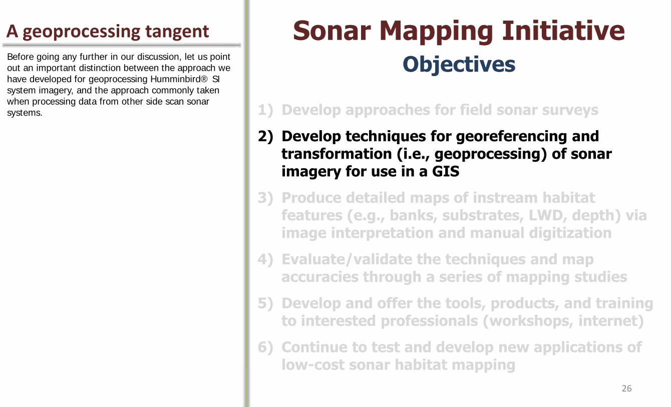
1) Develop approaches for field sonar surveys

2) Develop techniques for georeferencing and transformation (i.e., geoprocessing) of sonar imagery for use in a GIS

3) Produce detailed maps of instream habitat features (e.g., banks, substrates, LWD, depth) via image interpretation and manual digitization

4) Evaluate/validate the techniques and map accuracies through a series of mapping studies

5) Develop and offer the tools, products, and training to interested professionals (workshops, internet)

6) Continue to test and develop new applications of low-cost sonar habitat mapping

Before going any further in our discussion, let us point out an important distinction between the approach we have developed for geoprocessing Humminbird® SI system imagery, and the approach commonly taken when processing data from other side scan sonar systems.

26

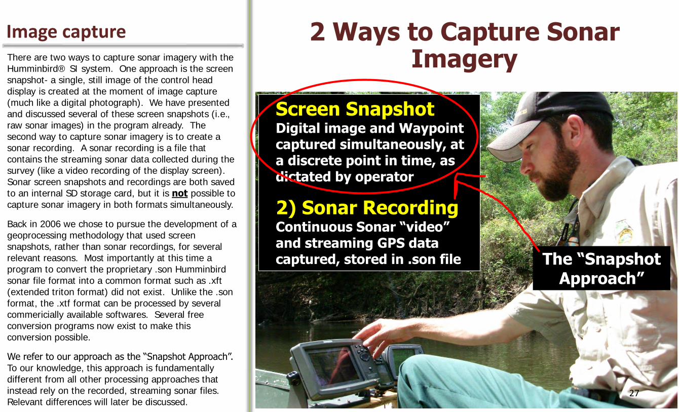
Image capture 2 Ways to Capture Sonar Imagery There are two ways to capture sonar imagery with the

Humminbird® SI system. One approach is the screen snapshot- a single, still image of the control head display is created at the moment of image capture (much like a digital photograph). We have presented and discussed several of these screen snapshots (i.e., raw sonar images) in the program already. The second way to capture sonar imagery is to create a sonar recording. A sonar recording is a file that contains the streaming sonar data collected during the survey (like a video recording of the display screen). Sonar screen snapshots and recordings are both saved to an internal SD storage card, but it is not possible to capture sonar imagery in both formats simultaneously.

Back in 2006 we chose to pursue the development of a geoprocessing methodology that used screen snapshots, rather than sonar recordings, for several relevant reasons. Most importantly at this time a program to convert the proprietary .son Humminbird sonar file format into a common format such as .xft (extended triton format) did not exist. Unlike the .son format, the .xtf format can be processed by several commericially available softwares. Several free conversion programs now exist to make this conversion possible.

We refer to our approach as the “Snapshot Approach”. To our knowledge, this approach is fundamentally different from all other processing approaches that instead rely on the recorded, streaming sonar files. Relevant differences will later be discussed.

Screen Snapshot Digital image and Waypoint captured simultaneously, at a discrete point in time, as dictated by operator

2) Sonar Recording Continuous Sonar “video” and streaming GPS data captured, stored in .son file The “Snapshot

Approach”

27

Program sessions Workshop Format Back to the workshop sessions- in the final session of the workshop we will discuss the preparation and evaluation of GIS-based maps containing several layers of habitat feature data.

Session IV- Part A

Habitat Mapping

Session IV- Part B

LWD, Accuracy Assessment, Applications

28

Session I- Part A Let us begin with the Introduction to Side Scan Sonar.

Introduction to Side Scan Sonar

Program Session I- Part A

29

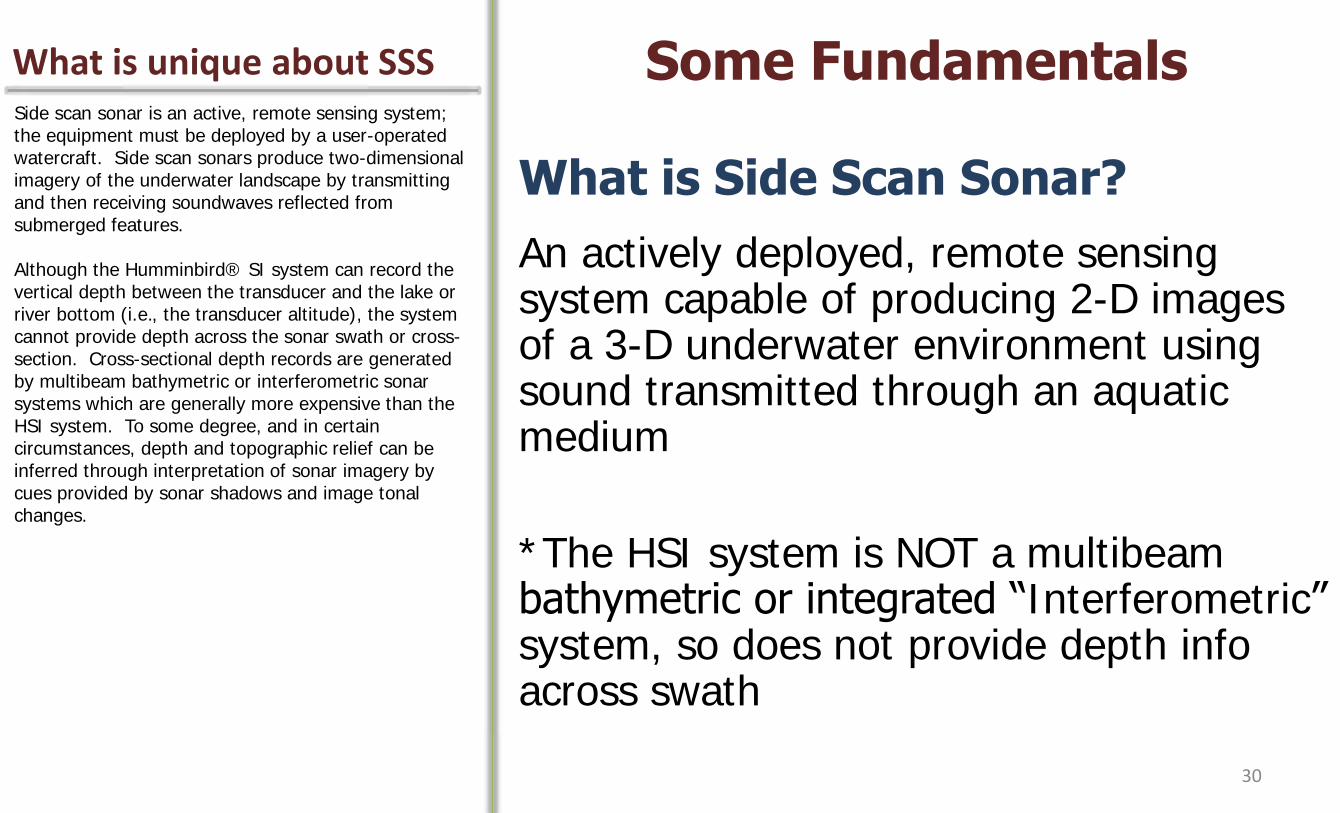
What is unique about SSS Some Fundamentals Side scan sonar is an active, remote sensing system; the equipment must be deployed by a user-operated watercraft. Side scan sonars produce two-dimensional imagery of the underwater landscape by transmitting and then receiving soundwaves reflected from submerged features. Although the Humminbird® SI system can record the vertical depth between the transducer and the lake or river bottom (i.e., the transducer altitude), the system cannot provide depth across the sonar swath or cross-section. Cross-sectional depth records are generated by multibeam bathymetric or interferometric sonar systems which are generally more expensive than the HSI system. To some degree, and in certain circumstances, depth and topographic relief can be inferred through interpretation of sonar imagery by cues provided by sonar shadows and image tonal changes.

What is Side Scan Sonar?

An actively deployed, remote sensing system capable of producing 2-D images of a 3-D underwater environment using sound transmitted through an aquatic medium

*The HSI system is NOT a multibeam bathymetric or integrated “Interferometric” system, so does not provide depth info across swath

30

SSS Components What Equipment is Involved? A few hardware components comprise the side scan system we operate. The Humminbird® SI system control head is a small console that can be mounted aboard the survey vessel. This control head houses an internal SD card for storage and transfer of sonar image data and files. The HSI system includes a small, foot-like transducer. If the transducer is destroyed during a mishap, a replacement can be purchased at a modest cost. Although some of the HSI models are packaged with a GPS receiver, we recommend the substitution of a hand-held unit like the Garmin GPSmap series device for purposes of easily recording and transferring a breadcrumb, track file that includes a depth observation at every track point. The last piece of hardware included in our set-up is a Seiko interval timer stopwatch. The stopwatch assists with the timing of sonar snapshot image capture during surveys, a process we will discuss in detail later.

Control head • Humminbird 900 or 1100 series

• SD Card for data storage

Transducer/Transmitter • XHS-9-HDSI-180-T (1100 series; $240

replacement cost)

Global Positioning System (GPS) • Garmin GPSmap 76, 76C, 76CSx ($150-

300)

• WAAS enabled (3-5m accuracy)

Seiko S057 Interval Timer ($85)

31

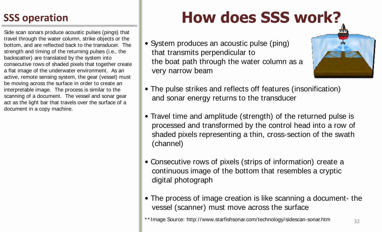
SSS operation How does SSS work? Side scan sonars produce acoustic pulses (pings) that travel through the water column, strike objects or the bottom, and are reflected back to the transducer. The strength and timing of the returning pulses (i.e., the backscatter) are translated by the system into consecutive rows of shaded pixels that together create a flat image of the underwater environment. As an active, remote sensing system, the gear (vessel) must be moving across the surface in order to create an interpretable image. The process is similar to the scanning of a document. The vessel and sonar gear act as the light bar that travels over the surface of a document in a copy machine.

• System produces an acoustic pulse (ping) that transmits perpendicular to the boat path through the water column as a very narrow beam

• The pulse strikes and reflects off features (insonification) and sonar energy returns to the transducer • Travel time and amplitude (strength) of the returned pulse is processed and transformed by the control head into a row of shaded pixels representing a thin, cross-section of the swath (channel) • Consecutive rows of pixels (strips of information) create a continuous image of the bottom that resembles a cryptic digital photograph • The process of image creation is like scanning a document- the vessel (scanner) must move across the surface

**Image Source: http://www.starfishsonar.com/technology/sidescan-sonar.htm 32

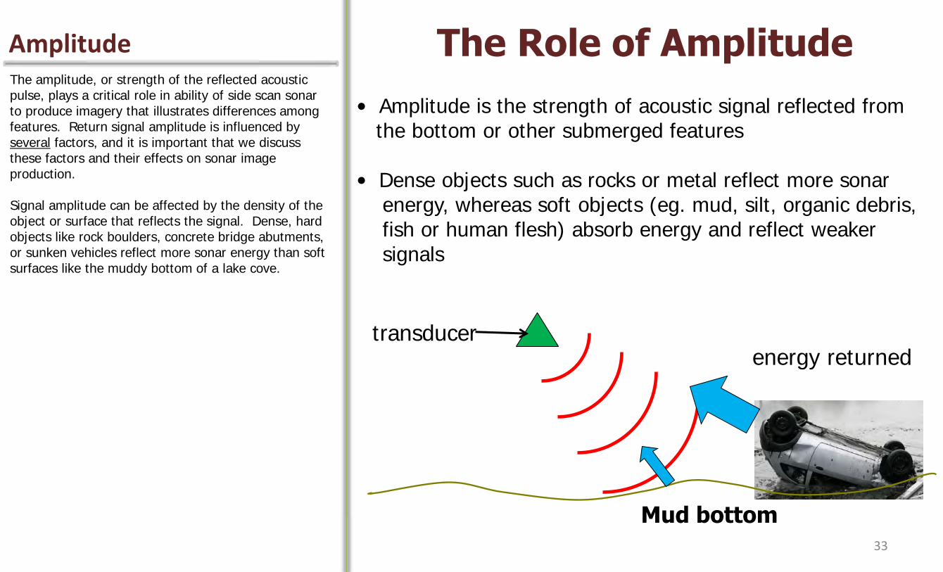
Amplitude The Role of Amplitude The amplitude, or strength of the reflected acoustic pulse, plays a critical role in ability of side scan sonar to produce imagery that illustrates differences among features. Return signal amplitude is influenced by several factors, and it is important that we discuss these factors and their effects on sonar image production. Signal amplitude can be affected by the density of the object or surface that reflects the signal. Dense, hard objects like rock boulders, concrete bridge abutments, or sunken vehicles reflect more sonar energy than soft surfaces like the muddy bottom of a lake cove.

• Amplitude is the strength of acoustic signal reflected from the bottom or other submerged features • Dense objects such as rocks or metal reflect more sonar energy, whereas soft objects (eg. mud, silt, organic debris, fish or human flesh) absorb energy and reflect weaker signals

transducer

Mud bottom

energy returned

33

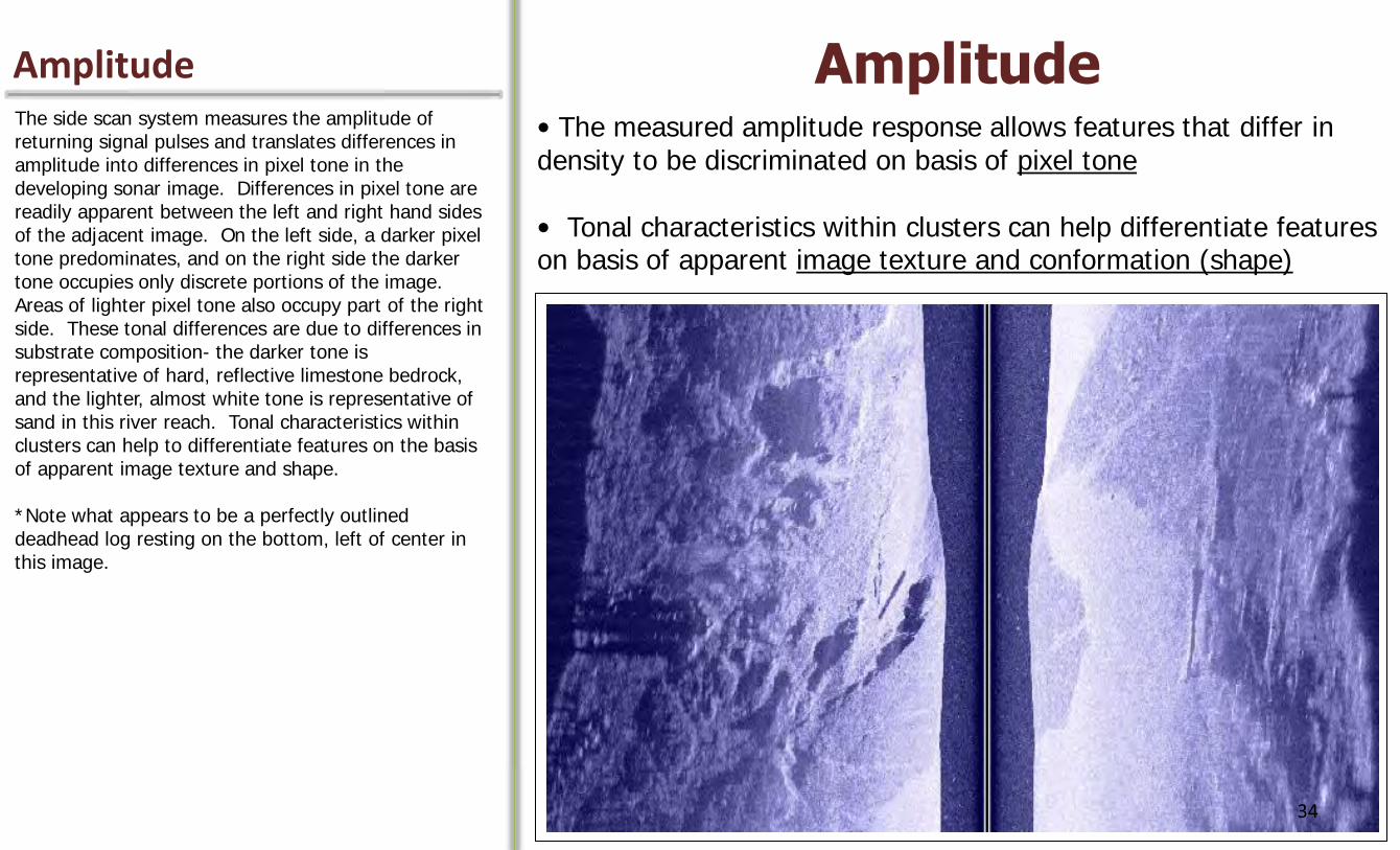
Amplitude Amplitude The side scan system measures the amplitude of returning signal pulses and translates differences in amplitude into differences in pixel tone in the developing sonar image. Differences in pixel tone are readily apparent between the left and right hand sides of the adjacent image. On the left side, a darker pixel tone predominates, and on the right side the darker tone occupies only discrete portions of the image. Areas of lighter pixel tone also occupy part of the right side. These tonal differences are due to differences in substrate composition- the darker tone is representative of hard, reflective limestone bedrock, and the lighter, almost white tone is representative of sand in this river reach. Tonal characteristics within clusters can help to differentiate features on the basis of apparent image texture and shape. *Note what appears to be a perfectly outlined deadhead log resting on the bottom, left of center in this image.

• The measured amplitude response allows features that differ in density to be discriminated on basis of pixel tone • Tonal characteristics within clusters can help differentiate features on basis of apparent image texture and conformation (shape)

34

Amplitude Amplitude Signal amplitude is also influenced by the angle at which the signal strikes an object or surface. This angle of incidence is also called the “grazing angle”. In the example provided here, we are scanning a stream whose bottom surface is entirely sand in composition, with sand bars providing some topographic relief. Although substrate composition is the same throughout, the leading edge of the sand bar (the edge facing the transducer) will reflect more sonar signal energy than the trailing, down-sloping edge of the sand bar. The backside of the sandbar reflects less sonar energy (i.e., lower signal amplitude) to the transducer, and we should expect to find tonal differences across the resulting sonar image.

• Amplitude is also influenced by other factors, such as the angle of incidence or “grazing angle”

transducer

Sand bar

Energy returned

35

Amplitude Amplitude The adjacent sonar image was captured in a river reach that appears to be composed entirely of sandy substrate. The ripple and dune patterning is characteristic of this substrate type in a lotic system (although sand does not always assume this appearance). Note the tonal change from left to right across this image. Toward the far right, the pixel tone darkens considerably, yet the rippling pattern indicative of sandy substrate remains. The reason for this difference in tone is likely a change in elevation (depth) across the image. It is likely that the left side of the image is relatively flat compared to the right side, which appears to be sloping away from the transducer (i.e., increasing in depth). We suspect that a trough, or deeper channel exists to the right hand side of the boat path. This image provides a good example of the effect of grazing angle on amplitude and image tone, and also how differences in tone can be interpreted to provide information on depth across the sonar swath. *When interpreting and discussing sonar imagery, it is important to emphasize that some degree of uncertainty often remains. The only way to confirm, for example, that a trough exists to the right of the boat in this image would be to obtain actual measurements of depth throughout this reach. In the paragraph above we use terms like “appears to be” and “likely” to indicate this uncertainty…but if we fail to use these terms in future discussions, know that some level of uncertainly exists whenever groundtruth data are incomplete or nonexistent.

Bottom sloping away from the transducer returns a weaker signal due to oblique grazing angles

*Note- The effect of bottom slope on grazing angle and signal return amplitude has particular relevance to the topic of automated image classification. As demonstrated above, pixel tone alone (i.e., the underlying numerical pixel values), cannot be used to correctly classify the substrate appearing in this image.

36

Amplitude Amplitude We have discussed density and grazing angle influences on amplitude and image tone, yet several additional factors can also effect signal return strength, including water density, suspended particulates like leaves, entrained gasses, and water turbulence. The raw image mosaic below was captured on the Coosa River during a frigid February morning in North Georgia. In the lower left a submerged pipe extends perpendicular to the river channel. This pipe is discharging warm effluent from a riverside power plant. The density differences between the warm plume and cold river water is scattering the sonar signal, producing image distortion along the bottom half of the image. This distortion extends far downstream (compare both sides of image, above and below pipe).

Amplitude can also be influenced by factors such as water density, enabling visualization of plumes of water of different temperature (for example), suspended particulates, entrained gasses, and turbulence (non-laminar flow)

37

Components of resolution Image Resolution / Quality Now that we hit on the topic of image distortion, let’s identify and discuss the two “principal components” of image resolution- along-track (or transverse) resolution and across-track resolution. Along-track resolution is associated with the dimension parallel to the boat path. Transverse resolution is the resolution associated with the dimension perpendicular to the boat path.

*Image Source: http://www.starfishsonar.com/technology/sidescan-sonar.htm

Two “principal components” of image resolution:

1. Along-track

(Transverse) Resolution

2. Across-track Resolution

38

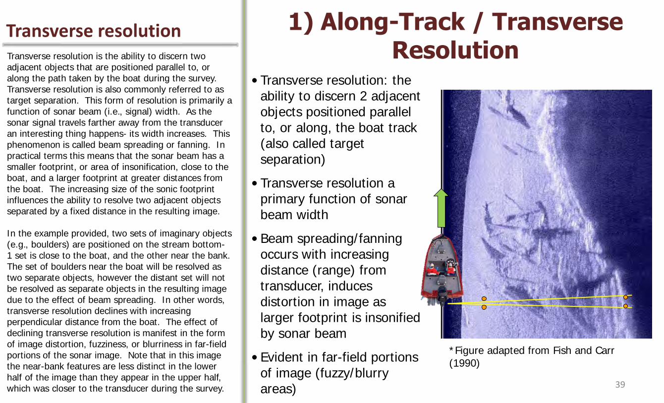
Transverse resolution 1) Along-Track / Transverse Resolution Transverse resolution is the ability to discern two

adjacent objects that are positioned parallel to, or along the path taken by the boat during the survey. Transverse resolution is also commonly referred to as target separation. This form of resolution is primarily a function of sonar beam (i.e., signal) width. As the sonar signal travels farther away from the transducer an interesting thing happens- its width increases. This phenomenon is called beam spreading or fanning. In practical terms this means that the sonar beam has a smaller footprint, or area of insonification, close to the boat, and a larger footprint at greater distances from the boat. The increasing size of the sonic footprint influences the ability to resolve two adjacent objects separated by a fixed distance in the resulting image. In the example provided, two sets of imaginary objects (e.g., boulders) are positioned on the stream bottom- 1 set is close to the boat, and the other near the bank. The set of boulders near the boat will be resolved as two separate objects, however the distant set will not be resolved as separate objects in the resulting image due to the effect of beam spreading. In other words, transverse resolution declines with increasing perpendicular distance from the boat. The effect of declining transverse resolution is manifest in the form of image distortion, fuzziness, or blurriness in far-field portions of the sonar image. Note that in this image the near-bank features are less distinct in the lower half of the image than they appear in the upper half, which was closer to the transducer during the survey.

• Transverse resolution: the ability to discern 2 adjacent objects positioned parallel to, or along, the boat track (also called target separation)

• Transverse resolution a primary function of sonar beam width

• Beam spreading/fanning occurs with increasing distance (range) from transducer, induces distortion in image as larger footprint is insonified by sonar beam

• Evident in far-field portions of image (fuzzy/blurry areas)

*Figure adapted from Fish and Carr 1990 *Figure adapted from Fish and Carr (1990)

39

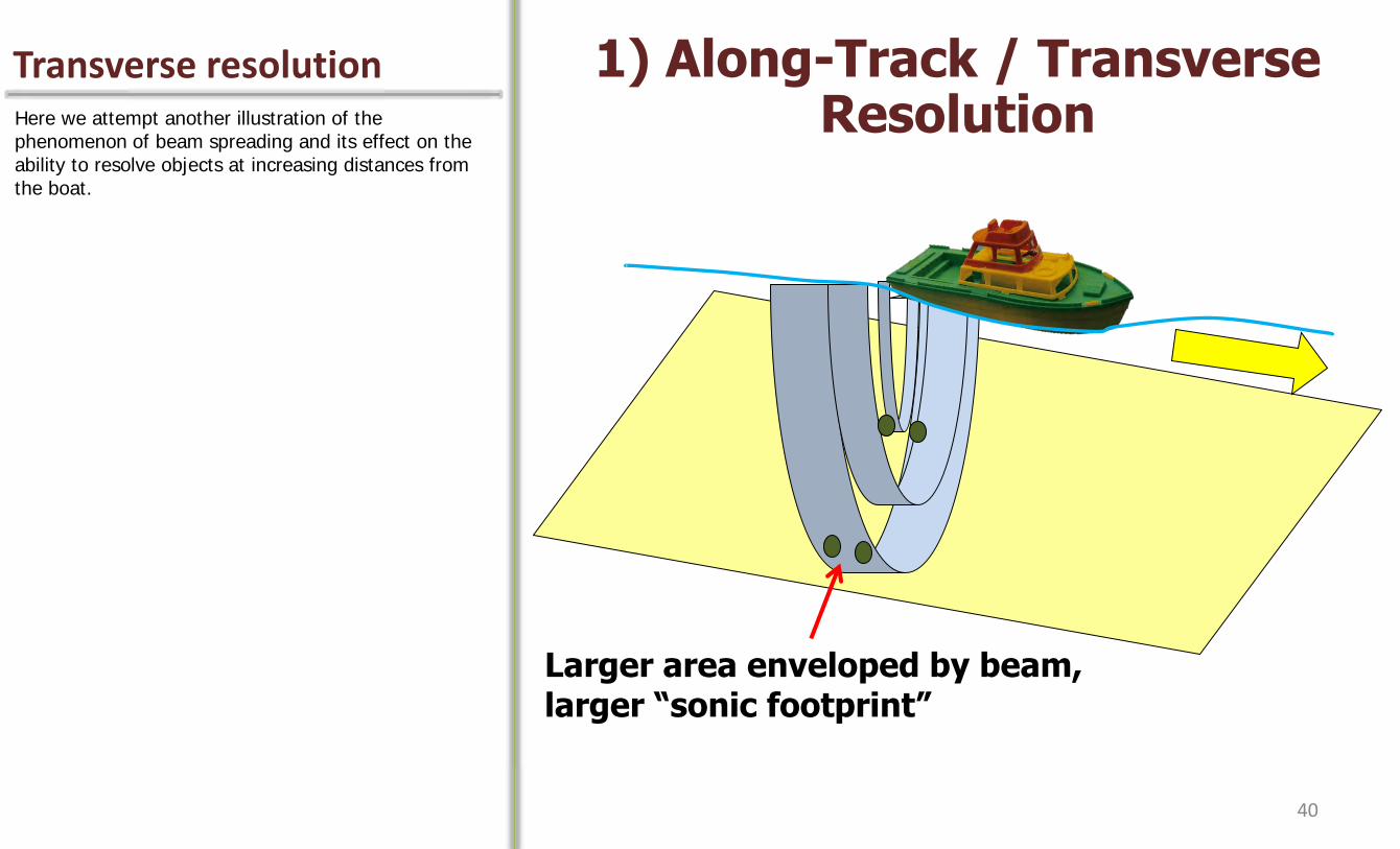
Transverse resolution 1) Along-Track / Transverse Resolution Here we attempt another illustration of the

phenomenon of beam spreading and its effect on the ability to resolve objects at increasing distances from the boat.

Larger area enveloped by beam, larger “sonic footprint”

40

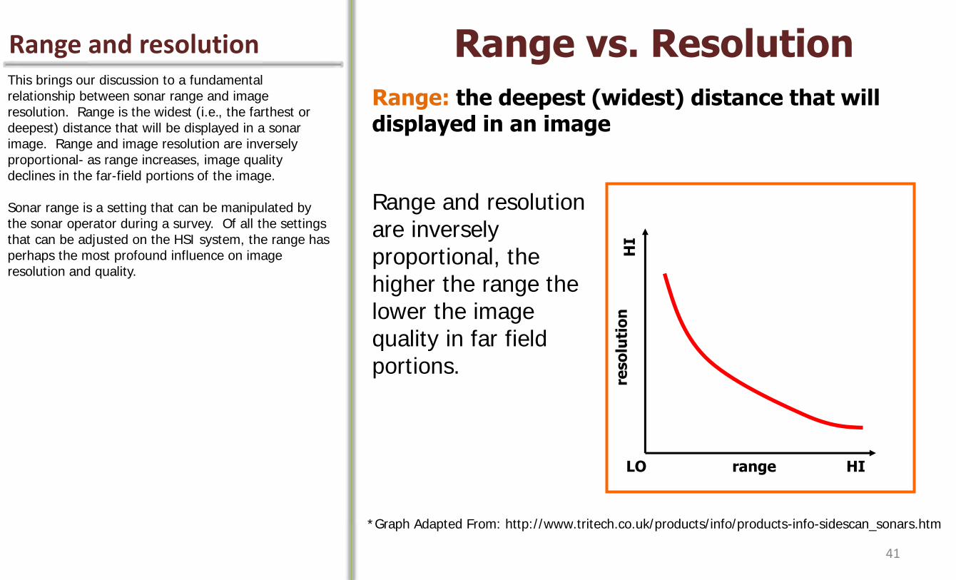
Range and resolution Range vs. Resolution This brings our discussion to a fundamental relationship between sonar range and image resolution. Range is the widest (i.e., the farthest or deepest) distance that will be displayed in a sonar image. Range and image resolution are inversely proportional- as range increases, image quality declines in the far-field portions of the image. Sonar range is a setting that can be manipulated by the sonar operator during a survey. Of all the settings that can be adjusted on the HSI system, the range has perhaps the most profound influence on image resolution and quality.

Range: the deepest (widest) distance that will displayed in an image

reso

luti

on

range HI LO

HI

Range and resolution are inversely proportional, the higher the range the lower the image quality in far field portions.

*Graph Adapted From: http://www.tritech.co.uk/products/info/products-info-sidescan_sonars.htm

41

Across-track resolution 2) Across-track / Range Resolution Let’s discuss the second principle component of image

resolution. Across-track resolution is defined as the ability to discern two adjacent objects positioned perpendicular to, or across the path taken by the boat during the survey. Across-track resolution is a function of sonar frequency, or pulse length. Lower sonar frequencies have a larger sonic footprint, reducing the resolving capability of the device. In this example, a low frequency pulse envelops both rocks simultaneously.

•Range resolution: the ability to discern 2 adjacent objects positioned perpendicular to, or across, the boat track

•Range resolution a function of pulse length (sonar frequency)

Lower frequency = larger sonic footprint

2 rocks

*Figure adapted from Fish and Carr (1990) 42

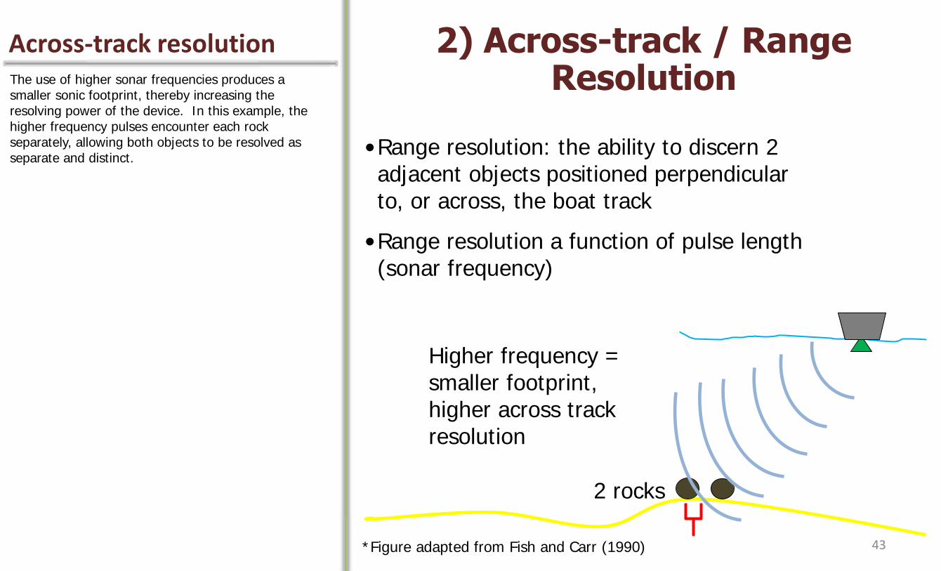
Across-track resolution 2) Across-track / Range Resolution The use of higher sonar frequencies produces a

smaller sonic footprint, thereby increasing the resolving power of the device. In this example, the higher frequency pulses encounter each rock separately, allowing both objects to be resolved as separate and distinct.

•Range resolution: the ability to discern 2 adjacent objects positioned perpendicular to, or across, the boat track

•Range resolution a function of pulse length (sonar frequency)

2 rocks

Higher frequency = smaller footprint, higher across track resolution

*Figure adapted from Fish and Carr (1990) 43

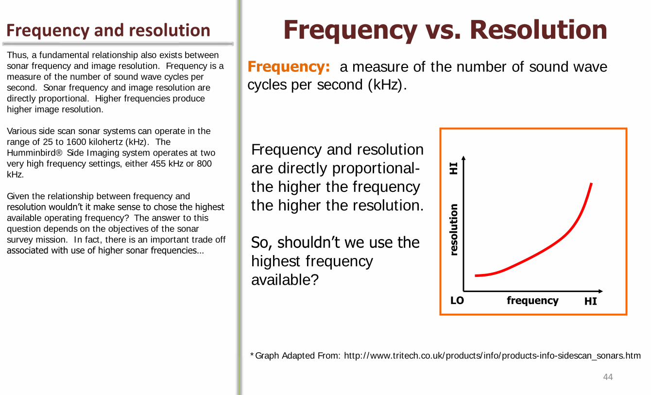
Frequency and resolution Frequency vs. Resolution Thus, a fundamental relationship also exists between sonar frequency and image resolution. Frequency is a measure of the number of sound wave cycles per second. Sonar frequency and image resolution are directly proportional. Higher frequencies produce higher image resolution. Various side scan sonar systems can operate in the range of 25 to 1600 kilohertz (kHz). The Humminbird® Side Imaging system operates at two very high frequency settings, either 455 kHz or 800 kHz. Given the relationship between frequency and resolution wouldn’t it make sense to chose the highest available operating frequency? The answer to this question depends on the objectives of the sonar survey mission. In fact, there is an important trade off associated with use of higher sonar frequencies…

Frequency: a measure of the number of sound wave cycles per second (kHz).

Frequency and resolution are directly proportional- the higher the frequency the higher the resolution. So, shouldn’t we use the highest frequency available?

Frequency vs. Range

frequency

reso

luti

on

LO HI

HI


44

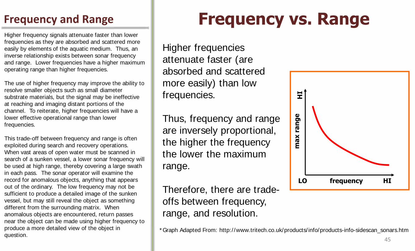
Frequency and Range Frequency vs. Range Higher frequency signals attenuate faster than lower frequencies as they are absorbed and scattered more easily by elements of the aquatic medium. Thus, an inverse relationship exists between sonar frequency and range. Lower frequencies have a higher maximum operating range than higher frequencies. The use of higher frequency may improve the ability to resolve smaller objects such as small diameter substrate materials, but the signal may be ineffective at reaching and imaging distant portions of the channel. To reiterate, higher frequencies will have a lower effective operational range than lower frequencies. This trade-off between frequency and range is often exploited during search and recovery operations. When vast areas of open water must be scanned in search of a sunken vessel, a lower sonar frequency will be used at high range, thereby covering a large swath in each pass. The sonar operator will examine the record for anomalous objects, anything that appears out of the ordinary. The low frequency may not be sufficient to produce a detailed image of the sunken vessel, but may still reveal the object as something different from the surrounding matrix. When anomalous objects are encountered, return passes near the object can be made using higher frequency to produce a more detailed view of the object in question.

Higher frequencies attenuate faster (are absorbed and scattered more easily) than low frequencies. Thus, frequency and range are inversely proportional, the higher the frequency the lower the maximum range. Therefore, there are trade-offs between frequency, range, and resolution.

ma

x r

an

ge

frequency HI LO

HI


45

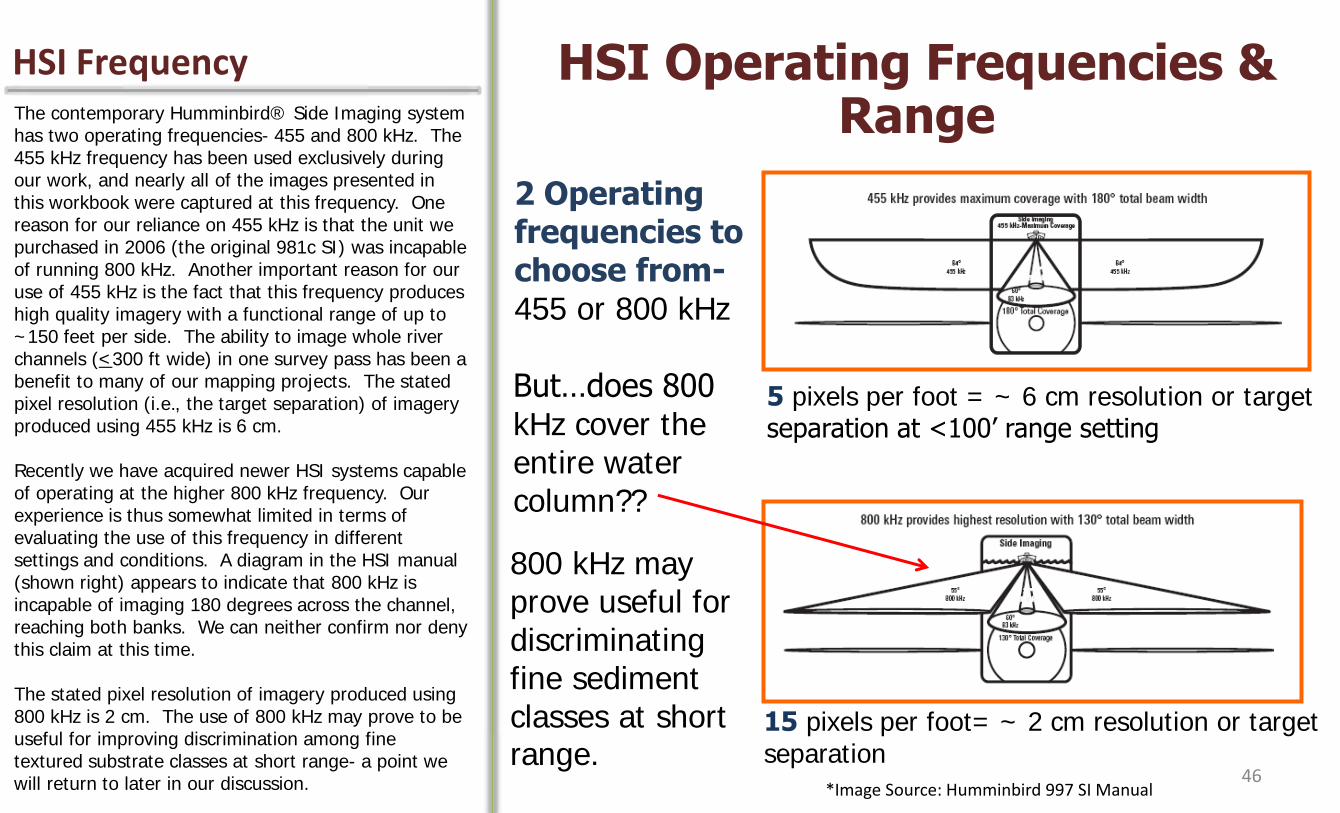
HSI Frequency HSI Operating Frequencies & Range The contemporary Humminbird® Side Imaging system

has two operating frequencies- 455 and 800 kHz. The 455 kHz frequency has been used exclusively during our work, and nearly all of the images presented in this workbook were captured at this frequency. One reason for our reliance on 455 kHz is that the unit we purchased in 2006 (the original 981c SI) was incapable of running 800 kHz. Another important reason for our use of 455 kHz is the fact that this frequency produces high quality imagery with a functional range of up to ~150 feet per side. The ability to image whole river channels (<300 ft wide) in one survey pass has been a benefit to many of our mapping projects. The stated pixel resolution (i.e., the target separation) of imagery produced using 455 kHz is 6 cm. Recently we have acquired newer HSI systems capable of operating at the higher 800 kHz frequency. Our experience is thus somewhat limited in terms of evaluating the use of this frequency in different settings and conditions. A diagram in the HSI manual (shown right) appears to indicate that 800 kHz is incapable of imaging 180 degrees across the channel, reaching both banks. We can neither confirm nor deny this claim at this time. The stated pixel resolution of imagery produced using 800 kHz is 2 cm. The use of 800 kHz may prove to be useful for improving discrimination among fine textured substrate classes at short range- a point we will return to later in our discussion.

5 pixels per foot = ~ 6 cm resolution or target separation at <100’ range setting

15 pixels per foot= ~ 2 cm resolution or target separation

2 Operating frequencies to choose from- 455 or 800 kHz

But…does 800 kHz cover the entire water column??

800 kHz may prove useful for discriminating fine sediment classes at short range.

*Image Source: Humminbird 997 SI Manual 46

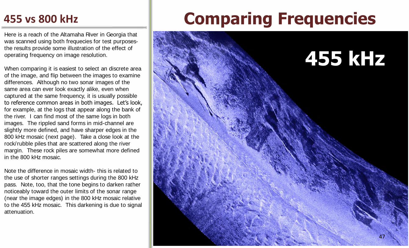
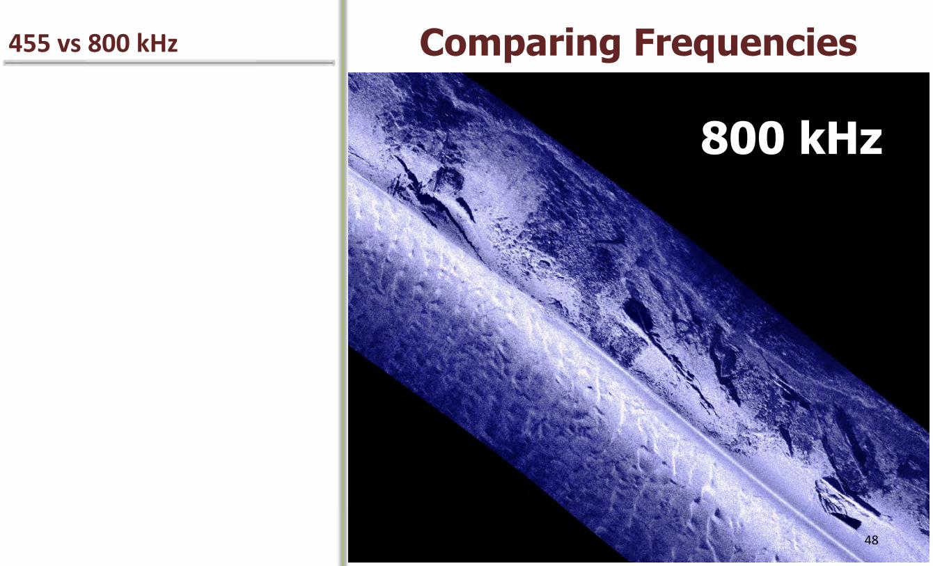
455 vs 800 kHz Here is a reach of the Altamaha River in Georgia that was scanned using both frequecies for test purposes- the results provide some illustration of the effect of operating frequency on image resolution. When comparing it is easiest to select an discrete area of the image, and flip between the images to examine differences. Although no two sonar images of the same area can ever look exactly alike, even when captured at the same frequency, it is usually possible to reference common areas in both images. Let’s look, for example, at the logs that appear along the bank of the river. I can find most of the same logs in both images. The rippled sand forms in mid-channel are slightly more defined, and have sharper edges in the 800 kHz mosaic (next page). Take a close look at the rock/rubble piles that are scattered along the river margin. These rock piles are somewhat more defined in the 800 kHz mosaic. Note the difference in mosaic width- this is related to the use of shorter ranges settings during the 800 kHz pass. Note, too, that the tone begins to darken rather noticeably toward the outer limits of the sonar range (near the image edges) in the 800 kHz mosaic relative to the 455 kHz mosaic. This darkening is due to signal attenuation.

455 kHz

Comparing Frequencies

47

455 vs 800 kHz

455 kHz

Comparing Frequencies

800 kHz

48

455 vs 800 kHz

455 kHz 800 kHz

Comparing Frequencies Here we display another reach of the Altamaha River for purposes of comparing sonar frequencies. In this image a nice cache of logs exists in the middle of the image. An expansive area of fine rocky substrate (likely cobble-sized material with some gravels) is distributed along the upper portion of the image. A vast area of migrating sand dunes and ripples occupies the lower half of the image. To a trained eye, these features are rather obvious in the 455 kHz mosaic.

455 kHz

49

Which frequency to use?

455 kHz 800 kHz

Comparing Frequencies The use of 800 kHz sharpens up the definition on some of the notable features, like the log cache, the cobble deposits, and the sand ripples. Whether the improvement in resolution is worth the expensive of the reduction in range is debatable. On other occasions we have observed a strong effect of water column turbulence and debris on the imaging performance of 800 kHz. The examples provided here represent results obtained during favorable imaging conditions. We encourage you to experiment with both frequencies during the survey planning phase, and critically evaluate performance with respect to meeting the specific needs and objectives of your sonar survey project.

800 kHz

50

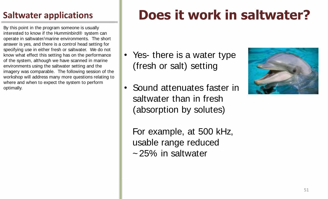
Saltwater applications Does it work in saltwater? By this point in the program someone is usually interested to know if the Humminbird® system can operate in saltwater/marine environments. The short answer is yes, and there is a control head setting for specifying use in either fresh or saltwater. We do not know what effect this setting has on the performance of the system, although we have scanned in marine environments using the saltwater setting and the imagery was comparable. The following session of the workshop will address many more questions relating to where and when to expect the system to perform optimally.

• Yes- there is a water type (fresh or salt) setting

• Sound attenuates faster in saltwater than in fresh (absorption by solutes)

For example, at 500 kHz, usable range reduced ~25% in saltwater

51

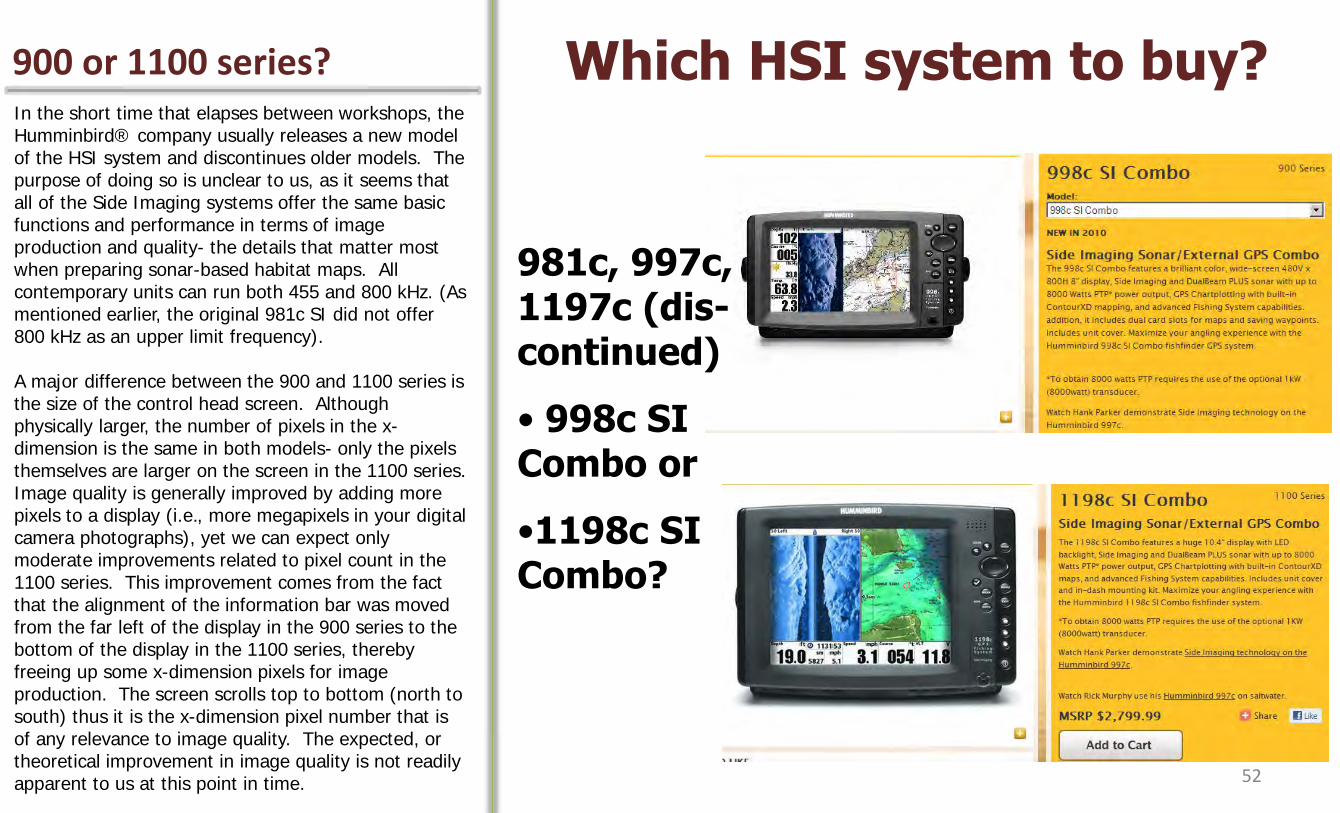
900 or 1100 series? Which HSI system to buy? In the short time that elapses between workshops, the Humminbird® company usually releases a new model of the HSI system and discontinues older models. The purpose of doing so is unclear to us, as it seems that all of the Side Imaging systems offer the same basic functions and performance in terms of image production and quality- the details that matter most when preparing sonar-based habitat maps. All contemporary units can run both 455 and 800 kHz. (As mentioned earlier, the original 981c SI did not offer 800 kHz as an upper limit frequency). A major difference between the 900 and 1100 series is the size of the control head screen. Although physically larger, the number of pixels in the x-dimension is the same in both models- only the pixels themselves are larger on the screen in the 1100 series. Image quality is generally improved by adding more pixels to a display (i.e., more megapixels in your digital camera photographs), yet we can expect only moderate improvements related to pixel count in the 1100 series. This improvement comes from the fact that the alignment of the information bar was moved from the far left of the display in the 900 series to the bottom of the display in the 1100 series, thereby freeing up some x-dimension pixels for image production. The screen scrolls top to bottom (north to south) thus it is the x-dimension pixel number that is of any relevance to image quality. The expected, or theoretical improvement in image quality is not readily apparent to us at this point in time.

981c, 997c, 1197c (dis-continued)

• 998c SI Combo or

•1198c SI Combo?

52

Additional references For More Information The body of literature that exists on the topic of side scan sonar is not very extensive, but we have found the two Fish and Carr books to be very interesting and insightful. Fish and Carr (1990) contains a chapter on theory of operation that we found to be very helpful in preparing portions of this session. On the other hand there are several informal sources for information on the Humminbird® system available online via the two forums listed here. One site is officially endorsed by Humminbird® and the other is an unofficial site. Both are frequented by passionate, HSI devotees who post on a variety of topics. These forums contain lengthy discussions and users freely offer advice and recommendations. Representatives of the Humminbird® company also post responses to user inquiries at these sites. This concludes Session I-Part A of the workshop.

• www.sideimagingsoft.com

• http://www.xumba.scholleco.com/

• Fish, J. P. and H. A. Carr. 1990. Sound Underwater Images- A guide to the generation and interpretation of side scan sonar data. Lower Cape Publishing, Orleans, MA.

• Fish, J. P. and H. A. Carr. 2001. Sound Reflections- Advanced applications of side scan sonar. Lower Cape Publishing, Orleans, MA.

• Fisheries Acoustics, Theory and Practice. 2005. J. Simmonds and D. MacLennan. Blackwell Publishing.

53

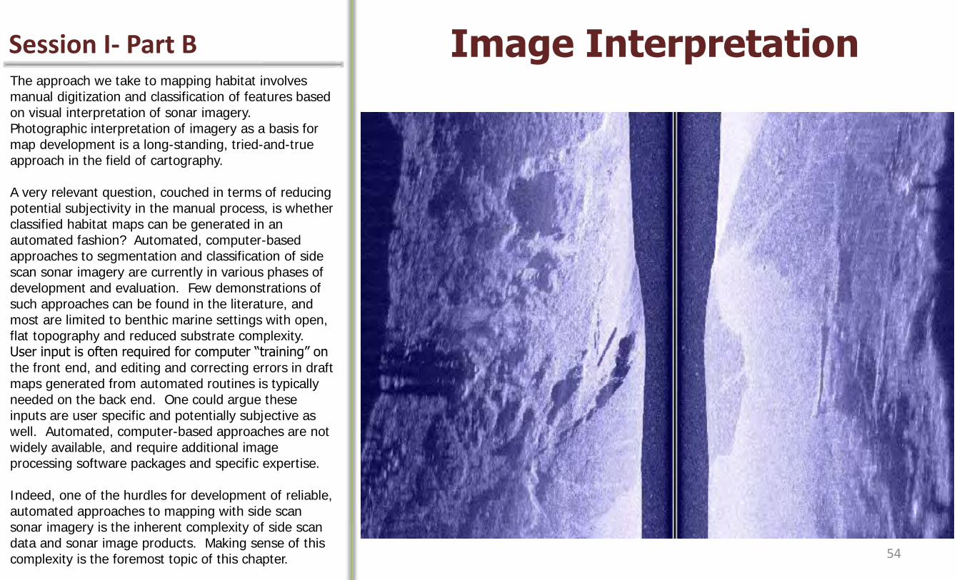
Session I- Part B Image Interpretation The approach we take to mapping habitat involves manual digitization and classification of features based on visual interpretation of sonar imagery. Photographic interpretation of imagery as a basis for map development is a long-standing, tried-and-true approach in the field of cartography. A very relevant question, couched in terms of reducing potential subjectivity in the manual process, is whether classified habitat maps can be generated in an automated fashion? Automated, computer-based approaches to segmentation and classification of side scan sonar imagery are currently in various phases of development and evaluation. Few demonstrations of such approaches can be found in the literature, and most are limited to benthic marine settings with open, flat topography and reduced substrate complexity. User input is often required for computer “training” on the front end, and editing and correcting errors in draft maps generated from automated routines is typically needed on the back end. One could argue these inputs are user specific and potentially subjective as well. Automated, computer-based approaches are not widely available, and require additional image processing software packages and specific expertise. Indeed, one of the hurdles for development of reliable, automated approaches to mapping with side scan sonar imagery is the inherent complexity of side scan data and sonar image products. Making sense of this complexity is the foremost topic of this chapter. 54

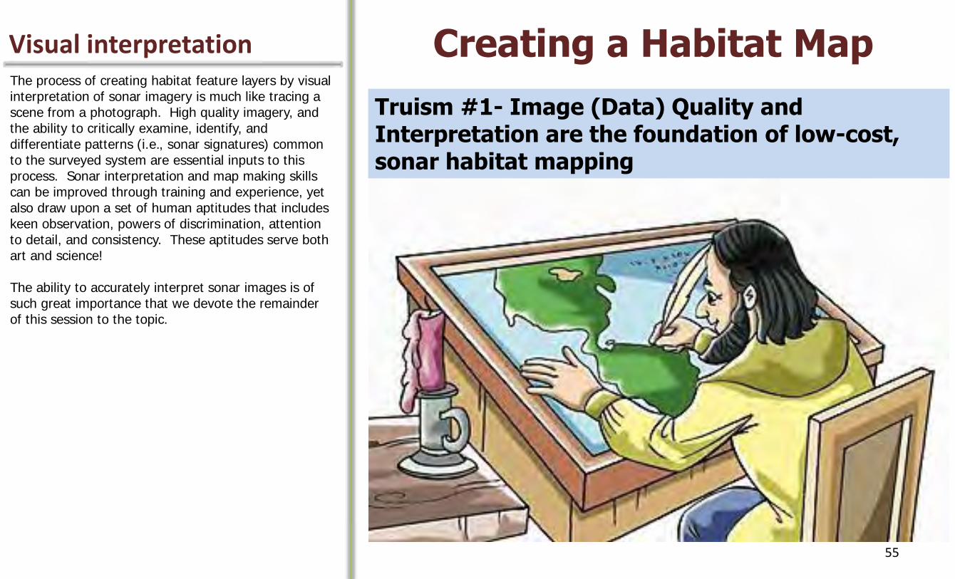
Visual interpretation Creating a Habitat Map The process of creating habitat feature layers by visual interpretation of sonar imagery is much like tracing a scene from a photograph. High quality imagery, and the ability to critically examine, identify, and differentiate patterns (i.e., sonar signatures) common to the surveyed system are essential inputs to this process. Sonar interpretation and map making skills can be improved through training and experience, yet also draw upon a set of human aptitudes that includes keen observation, powers of discrimination, attention to detail, and consistency. These aptitudes serve both art and science! The ability to accurately interpret sonar images is of such great importance that we devote the remainder of this session to the topic.

Truism #1- Image (Data) Quality and Interpretation are the foundation of low-cost, sonar habitat mapping

55

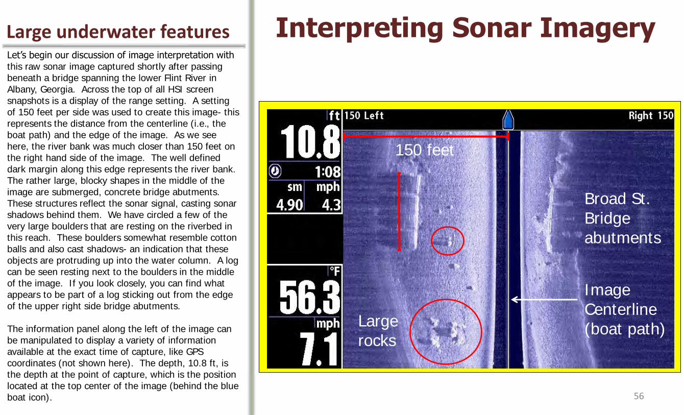
Interpreting Sonar Imagery Let’s begin our discussion of image interpretation with

this raw sonar image captured shortly after passing beneath a bridge spanning the lower Flint River in Albany, Georgia. Across the top of all HSI screen snapshots is a display of the range setting. A setting of 150 feet per side was used to create this image- this represents the distance from the centerline (i.e., the boat path) and the edge of the image. As we see here, the river bank was much closer than 150 feet on the right hand side of the image. The well defined dark margin along this edge represents the river bank. The rather large, blocky shapes in the middle of the image are submerged, concrete bridge abutments. These structures reflect the sonar signal, casting sonar shadows behind them. We have circled a few of the very large boulders that are resting on the riverbed in this reach. These boulders somewhat resemble cotton balls and also cast shadows- an indication that these objects are protruding up into the water column. A log can be seen resting next to the boulders in the middle of the image. If you look closely, you can find what appears to be part of a log sticking out from the edge of the upper right side bridge abutments. The information panel along the left of the image can be manipulated to display a variety of information available at the exact time of capture, like GPS coordinates (not shown here). The depth, 10.8 ft, is the depth at the point of capture, which is the position located at the top center of the image (behind the blue boat icon).

Large rocks

150 feet

Large underwater features

Broad St. Bridge abutments

Image Centerline (boat path)

56

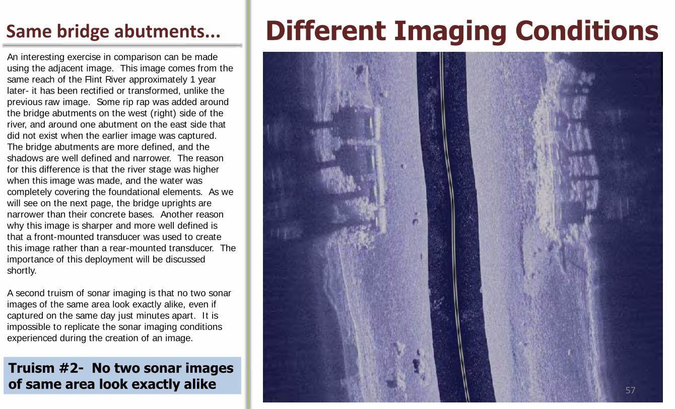
Same bridge abutments... Different Imaging Conditions An interesting exercise in comparison can be made using the adjacent image. This image comes from the same reach of the Flint River approximately 1 year later- it has been rectified or transformed, unlike the previous raw image. Some rip rap was added around the bridge abutments on the west (right) side of the river, and around one abutment on the east side that did not exist when the earlier image was captured. The bridge abutments are more defined, and the shadows are well defined and narrower. The reason for this difference is that the river stage was higher when this image was made, and the water was completely covering the foundational elements. As we will see on the next page, the bridge uprights are narrower than their concrete bases. Another reason why this image is sharper and more well defined is that a front-mounted transducer was used to create this image rather than a rear-mounted transducer. The importance of this deployment will be discussed shortly. A second truism of sonar imaging is that no two sonar images of the same area look exactly alike, even if captured on the same day just minutes apart. It is impossible to replicate the sonar imaging conditions experienced during the creation of an image.

Truism #2- No two sonar images of same area look exactly alike 57

Low water conditions The Bridge Abutments Here is a digital photo of the west side bridge abutments of the bridge over the Flint River taken during low water conditions. The difference between abutment base and uprights is plain to see, as is the representative signature of these structures in the sonar image.

Sonar Shadows

58

Texture difference Rip Rap This photo was taken while looking at rip rap (i.e., boulders) added to the bridge abutment area. The sonar signature of this material is clearly different from the surrounding riverbed.

59

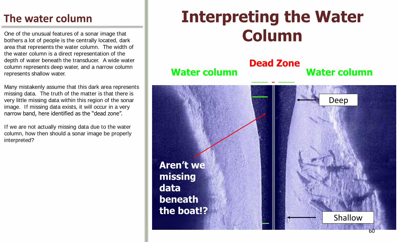
The water column Interpreting the Water Column One of the unusual features of a sonar image that

bothers a lot of people is the centrally located, dark area that represents the water column. The width of the water column is a direct representation of the depth of water beneath the transducer. A wide water column represents deep water, and a narrow column represents shallow water. Many mistakenly assume that this dark area represents missing data. The truth of the matter is that there is very little missing data within this region of the sonar image. If missing data exists, it will occur in a very narrow band, here identified as the “dead zone”. If we are not actually missing data due to the water column, how then should a sonar image be properly interpreted?

Water column Water column

Shallow

Deep

Aren’t we missing data beneath the boat!?

Dead Zone

60

The water column Objects directly beneath transducer To properly interpret sonar imagery with the water

column displayed we must imagine that both sides of the sonar image actually join together right down the middle of the image, as if the water column does not exist. Visual proof of this concept is occasionally obtained when the boat happens to pass directly over an object, or set of objects, like these boulders. The boulders appear as mirror objects on either side of the image. Imagine mentally removing the water column and stitching the two halves of the image together down the center- the modified image would have a series of three or so boulders that were located directly beneath the boat during the survey.

-Appear as mirror images on either side

61

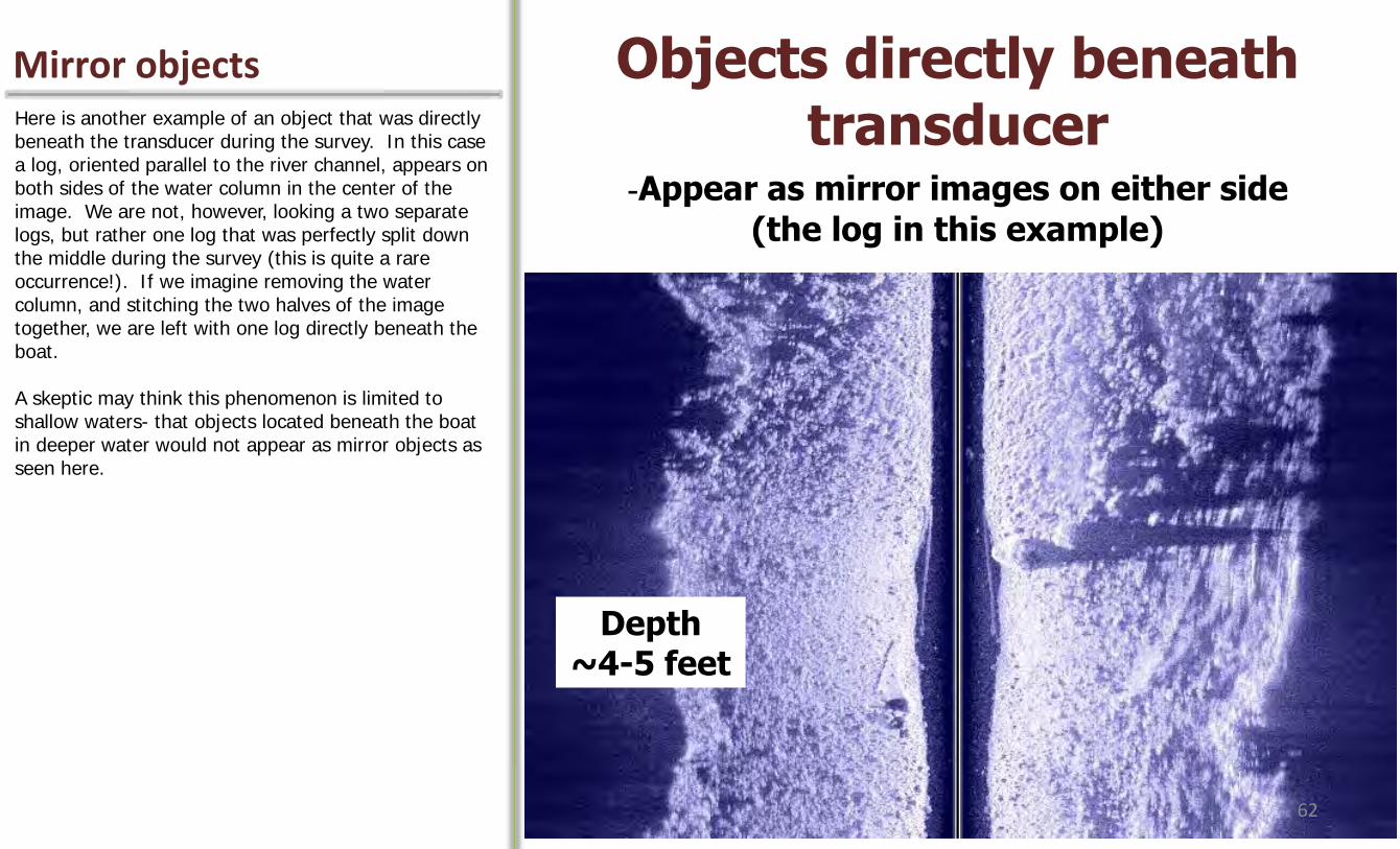
Mirror objects Objects directly beneath transducer Here is another example of an object that was directly

beneath the transducer during the survey. In this case a log, oriented parallel to the river channel, appears on both sides of the water column in the center of the image. We are not, however, looking a two separate logs, but rather one log that was perfectly split down the middle during the survey (this is quite a rare occurrence!). If we imagine removing the water column, and stitching the two halves of the image together, we are left with one log directly beneath the boat. A skeptic may think this phenomenon is limited to shallow waters- that objects located beneath the boat in deeper water would not appear as mirror objects as seen here.


(the log in this example)

Depth ~4-5 feet

62

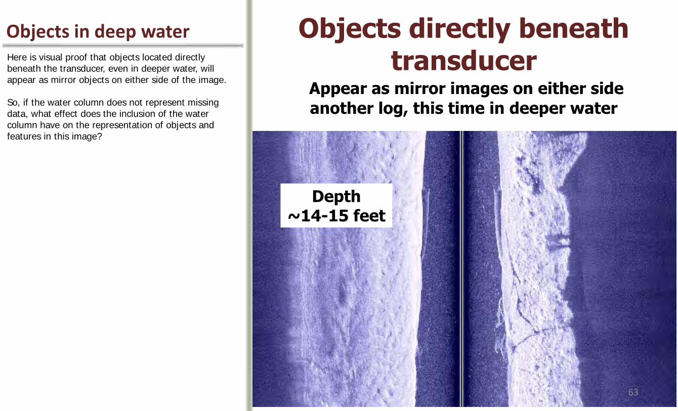
Objects in deep water Objects directly beneath transducer Here is visual proof that objects located directly

beneath the transducer, even in deeper water, will appear as mirror objects on either side of the image. So, if the water column does not represent missing data, what effect does the inclusion of the water column have on the representation of objects and features in this image?


another log, this time in deeper water

Depth ~14-15 feet

63

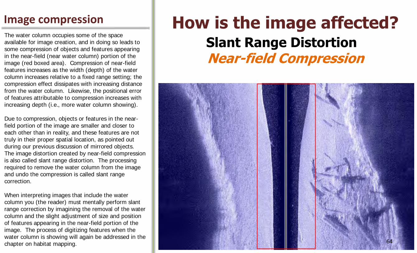
Image compression How is the image affected? The water column occupies some of the space available for image creation, and in doing so leads to some compression of objects and features appearing in the near-field (near water column) portion of the image (red boxed area). Compression of near-field features increases as the width (depth) of the water column increases relative to a fixed range setting; the compression effect dissipates with increasing distance from the water column. Likewise, the positional error of features attributable to compression increases with increasing depth (i.e., more water column showing). Due to compression, objects or features in the near-field portion of the image are smaller and closer to each other than in reality, and these features are not truly in their proper spatial location, as pointed out during our previous discussion of mirrored objects. The image distortion created by near-field compression is also called slant range distortion. The processing required to remove the water column from the image and undo the compression is called slant range correction. When interpreting images that include the water column you (the reader) must mentally perform slant range correction by imagining the removal of the water column and the slight adjustment of size and position of features appearing in the near-field portion of the image. The process of digitizing features when the water column is showing will again be addressed in the chapter on habitat mapping.

Slant Range Distortion Near-field Compression

64

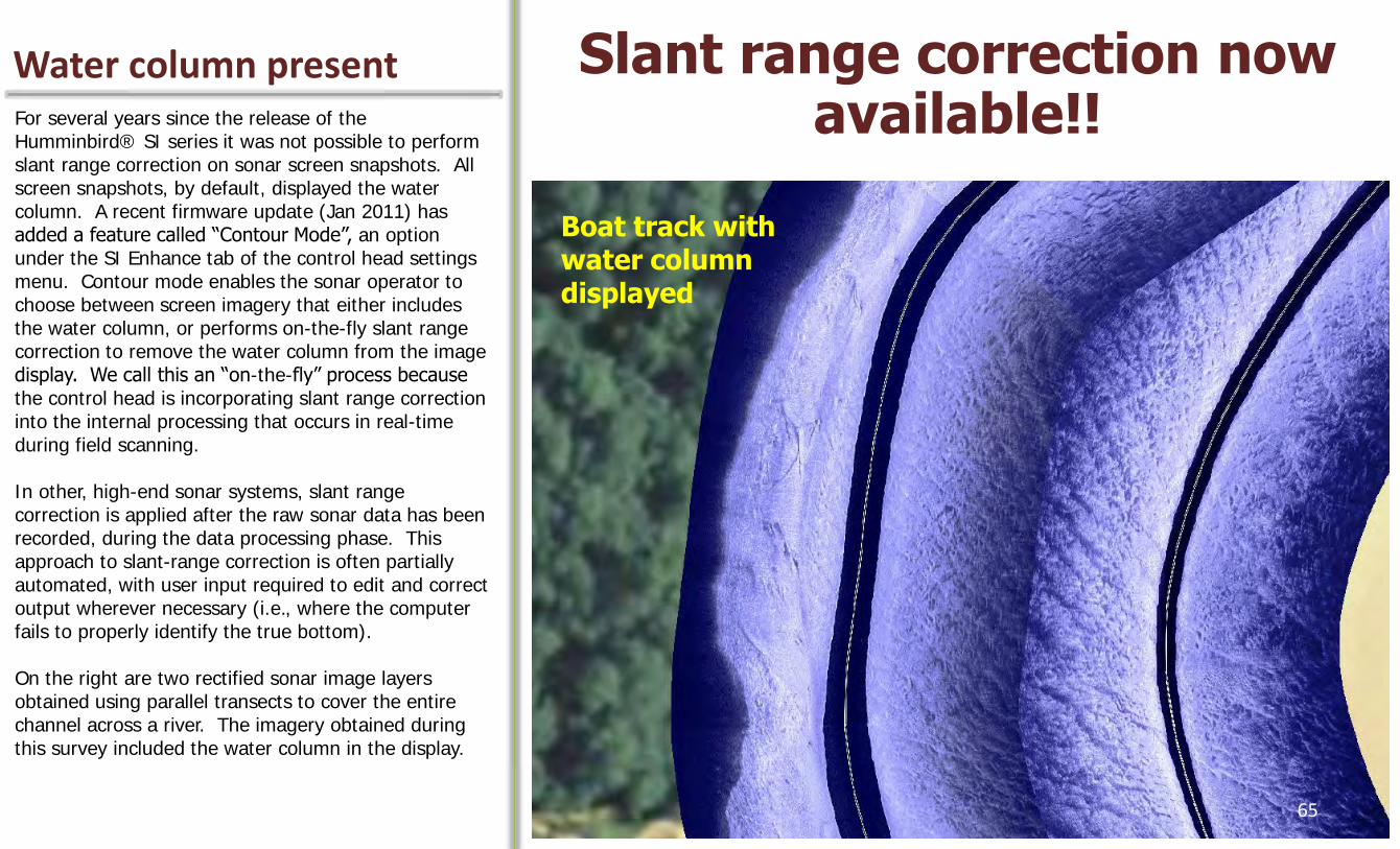
Water column present Slant range correction now available!! For several years since the release of the

Humminbird® SI series it was not possible to perform slant range correction on sonar screen snapshots. All screen snapshots, by default, displayed the water column. A recent firmware update (Jan 2011) has added a feature called “Contour Mode”, an option under the SI Enhance tab of the control head settings menu. Contour mode enables the sonar operator to choose between screen imagery that either includes the water column, or performs on-the-fly slant range correction to remove the water column from the image display. We call this an “on-the-fly” process because the control head is incorporating slant range correction into the internal processing that occurs in real-time during field scanning. In other, high-end sonar systems, slant range correction is applied after the raw sonar data has been recorded, during the data processing phase. This approach to slant-range correction is often partially automated, with user input required to edit and correct output wherever necessary (i.e., where the computer fails to properly identify the true bottom). On the right are two rectified sonar image layers obtained using parallel transects to cover the entire channel across a river. The imagery obtained during this survey included the water column in the display.

Boat track with water column displayed

65

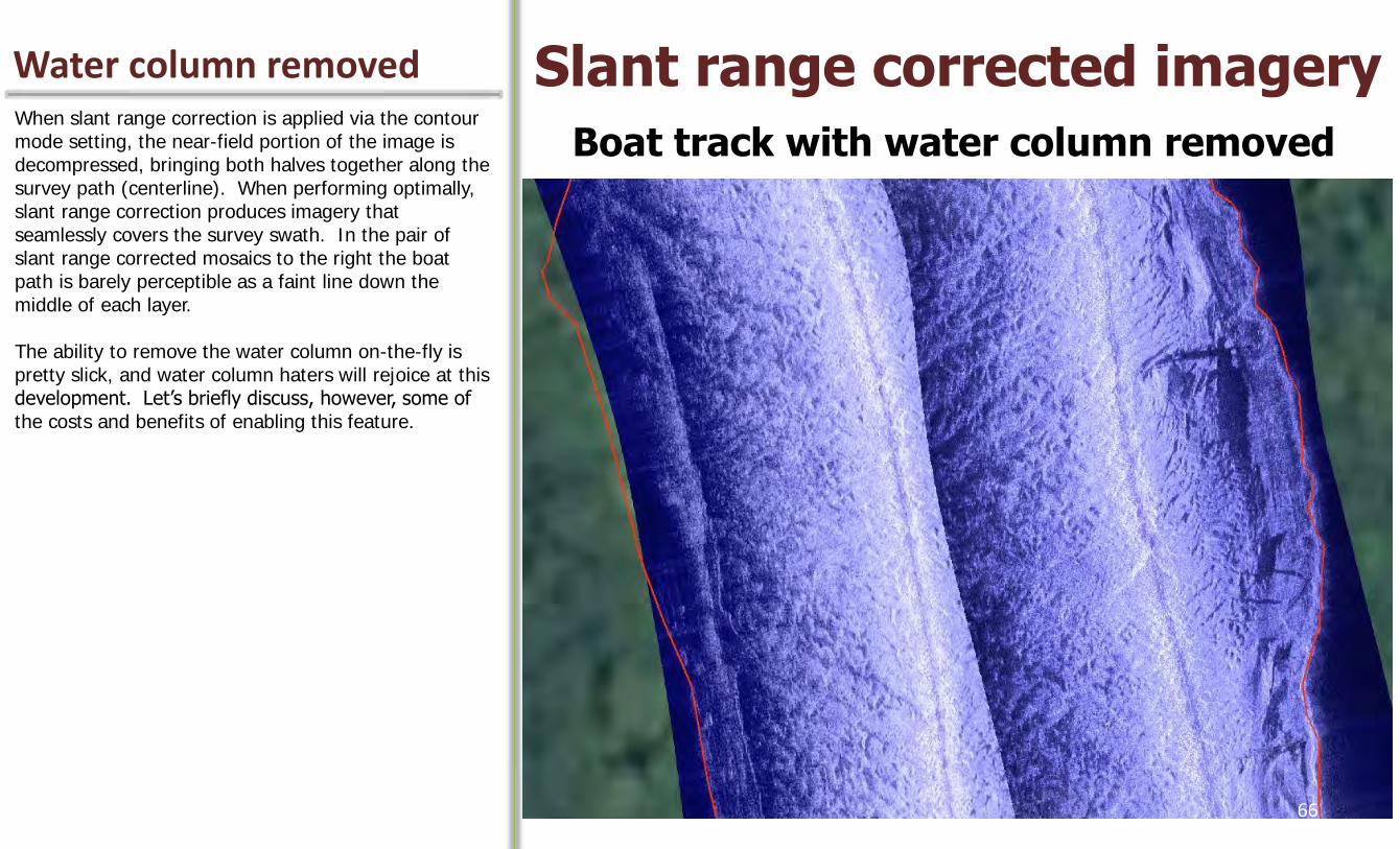
Water column removed Slant range corrected imagery

Boat track with water column removed When slant range correction is applied via the contour mode setting, the near-field portion of the image is decompressed, bringing both halves together along the survey path (centerline). When performing optimally, slant range correction produces imagery that seamlessly covers the survey swath. In the pair of slant range corrected mosaics to the right the boat path is barely perceptible as a faint line down the middle of each layer. The ability to remove the water column on-the-fly is pretty slick, and water column haters will rejoice at this development. Let’s briefly discuss, however, some of the costs and benefits of enabling this feature.

66

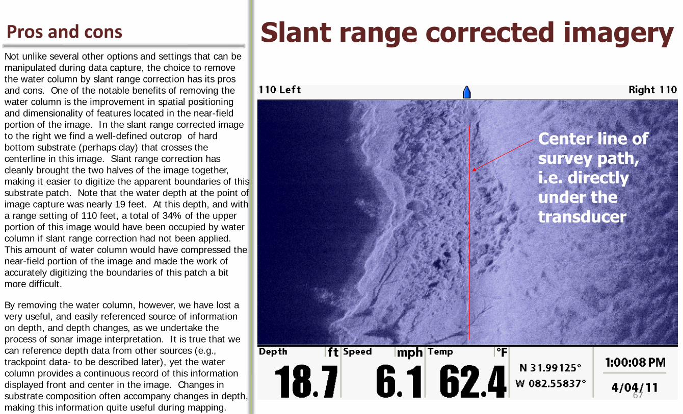
Pros and cons Slant range corrected imagery Not unlike several other options and settings that can be manipulated during data capture, the choice to remove the water column by slant range correction has its pros and cons. One of the notable benefits of removing the water column is the improvement in spatial positioning and dimensionality of features located in the near-field portion of the image. In the slant range corrected image to the right we find a well-defined outcrop of hard bottom substrate (perhaps clay) that crosses the centerline in this image. Slant range correction has cleanly brought the two halves of the image together, making it easier to digitize the apparent boundaries of this substrate patch. Note that the water depth at the point of image capture was nearly 19 feet. At this depth, and with a range setting of 110 feet, a total of 34% of the upper portion of this image would have been occupied by water column if slant range correction had not been applied. This amount of water column would have compressed the near-field portion of the image and made the work of accurately digitizing the boundaries of this patch a bit more difficult.

By removing the water column, however, we have lost a very useful, and easily referenced source of information on depth, and depth changes, as we undertake the process of sonar image interpretation. It is true that we can reference depth data from other sources (e.g., trackpoint data- to be described later), yet the water column provides a continuous record of this information displayed front and center in the image. Changes in substrate composition often accompany changes in depth, making this information quite useful during mapping.

Center line of survey path, i.e. directly under the transducer

67

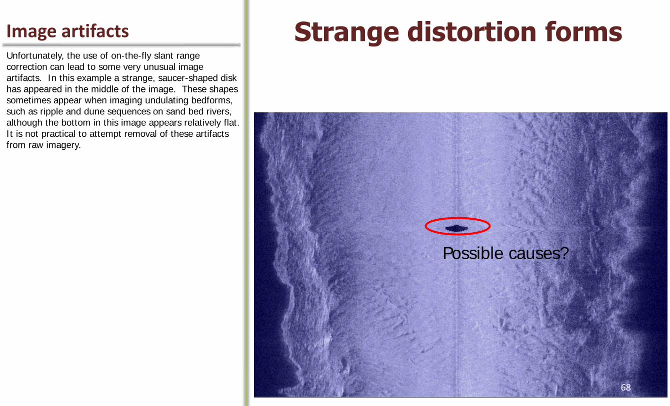
Image artifacts Strange distortion forms Unfortunately, the use of on-the-fly slant range correction can lead to some very unusual image artifacts. In this example a strange, saucer-shaped disk has appeared in the middle of the image. These shapes sometimes appear when imaging undulating bedforms, such as ripple and dune sequences on sand bed rivers, although the bottom in this image appears relatively flat. It is not practical to attempt removal of these artifacts from raw imagery.

Possible causes?

68

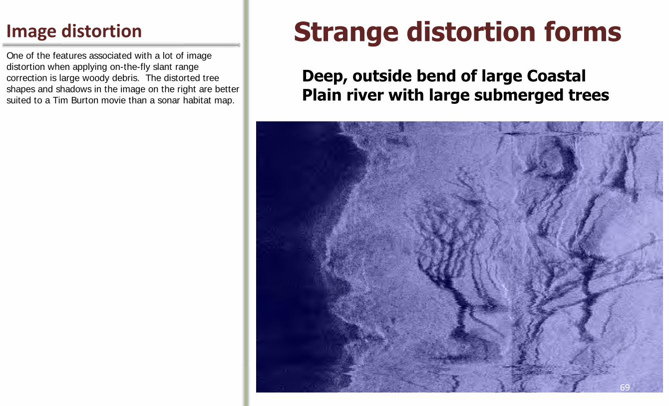
Image distortion Strange distortion forms One of the features associated with a lot of image distortion when applying on-the-fly slant range correction is large woody debris. The distorted tree shapes and shadows in the image on the right are better suited to a Tim Burton movie than a sonar habitat map.

Deep, outside bend of large Coastal Plain river with large submerged trees

69

Image distortions Strange distortion forms The distortion present in this image is downright horrible. If you had to spend more than a few minutes trying to map habitat from imagery like this you might end up puking on your shoes! What is going on here, and what might we learn from these examples regarding the judicious use of slant range correction with the Humminbird system?


70

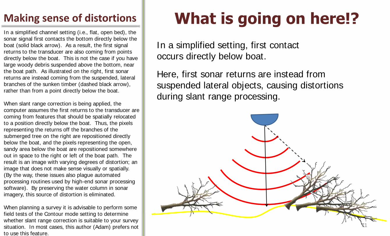
Making sense of distortions What is going on here!? In a simplified channel setting (i.e., flat, open bed), the sonar signal first contacts the bottom directly below the boat (solid black arrow). As a result, the first signal returns to the transducer are also coming from points directly below the boat. This is not the case if you have large woody debris suspended above the bottom, near the boat path. As illustrated on the right, first sonar returns are instead coming from the suspended, lateral branches of the sunken timber (dashed black arrow), rather than from a point directly below the boat. When slant range correction is being applied, the computer assumes the first returns to the transducer are coming from features that should be spatially relocated to a position directly below the boat. Thus, the pixels representing the returns off the branches of the submerged tree on the right are repositioned directly below the boat, and the pixels representing the open, sandy area below the boat are repositioned somewhere out in space to the right or left of the boat path. The result is an image with varying degrees of distortion; an image that does not make sense visually or spatially. (By the way, these issues also plague automated processing routines used by high-end sonar processing software). By preserving the water column in sonar imagery, this source of distortion is eliminated. When planning a survey it is advisable to perform some field tests of the Contour mode setting to determine whether slant range correction is suitable to your survey situation. In most cases, this author (Adam) prefers not to use this feature.

In a simplified setting, first contact occurs directly below boat.

Here, first sonar returns are instead from suspended lateral objects, causing distortions during slant range processing.

71

Classic substrates Rocky shoals and sand bar Now that we’ve covered some of the bases on water column and slant range correction, let’s look at some of the typical substrates we’ve encountered in surveys of streams of the Southeast Coastal Plain. The image from the right was captured in the lower Flint River. This river is characterized by extensive rocky shoals (primarily cobble to boulder sized material), sand flats, and reaches of flat, limestone bedrock exposures. On the right, we can see that the survey boat approached a rocky shoal, and charted a course over the shoal. The transducer came close, but did not strike, a few of the large, shallow boulders present in the shoal. As the boat approached this shoal, the shallow water and rock pile blocked and reflected the signal back to the boat, casting sonar shadows. These shadowed areas represent missing data that can be quantified during mapping. Note the difference between the large, coarse material predominant along the left side of the image, and the finer (yet still textured) rocky material on the right hand side of the image. This finer textured material is cobble-sized rock (according to the modified Wentworth particle size scheme). In the lower left hand corner of the image appears a smooth sand bar. The boundary between the sand and rocky shoal is strikingly obvious.


Cobble

Boulder

72

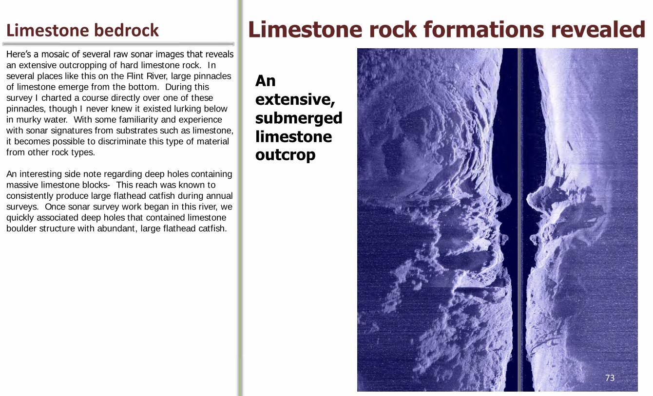
Limestone bedrock Limestone rock formations revealed Here’s a mosaic of several raw sonar images that reveals an extensive outcropping of hard limestone rock. In several places like this on the Flint River, large pinnacles of limestone emerge from the bottom. During this survey I charted a course directly over one of these pinnacles, though I never knew it existed lurking below in murky water. With some familiarity and experience with sonar signatures from substrates such as limestone, it becomes possible to discriminate this type of material from other rock types. An interesting side note regarding deep holes containing massive limestone blocks- This reach was known to consistently produce large flathead catfish during annual surveys. Once sonar survey work began in this river, we quickly associated deep holes that contained limestone boulder structure with abundant, large flathead catfish.

An extensive, submerged limestone outcrop

73

Sand formations Sand Dunes In rivers sandy substrate is often sculpted into beautiful dune and ripple patterns. Like winds that carry sand across the desert, currents carry sand downstream. This process creates characteristic bedforms that reveal the nature of the substrate.

Sand dunes along the bottom of the Flint River

74

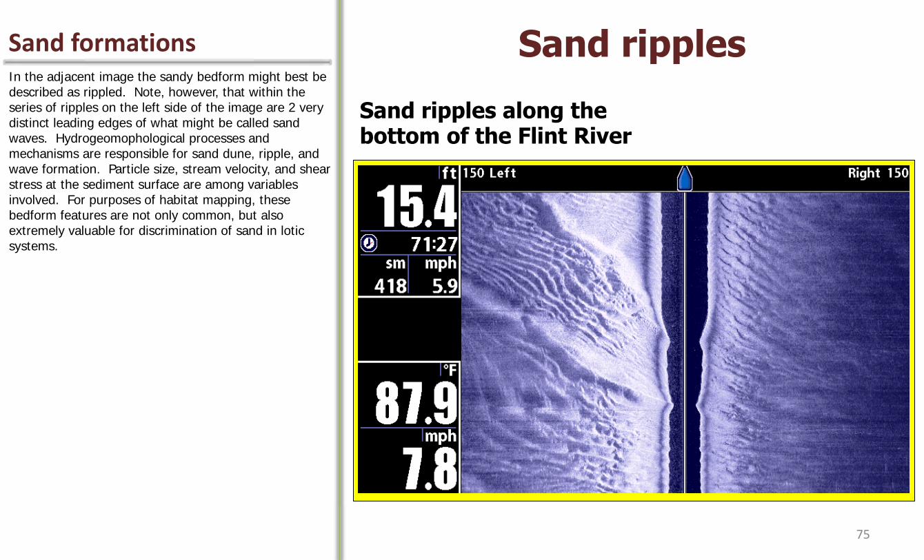
Sand formations Sand ripples In the adjacent image the sandy bedform might best be described as rippled. Note, however, that within the series of ripples on the left side of the image are 2 very distinct leading edges of what might be called sand waves. Hydrogeomophological processes and mechanisms are responsible for sand dune, ripple, and wave formation. Particle size, stream velocity, and shear stress at the sediment surface are among variables involved. For purposes of habitat mapping, these bedform features are not only common, but also extremely valuable for discrimination of sand in lotic systems.

Sand ripples along the bottom of the Flint River

75

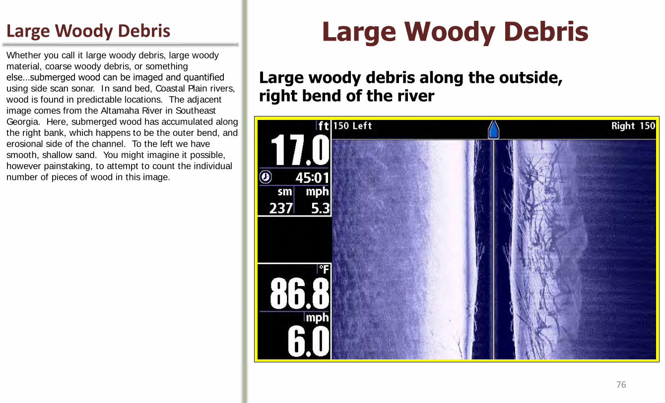
Large Woody Debris Large Woody Debris Whether you call it large woody debris, large woody material, coarse woody debris, or something else…submerged wood can be imaged and quantified using side scan sonar. In sand bed, Coastal Plain rivers, wood is found in predictable locations. The adjacent image comes from the Altamaha River in Southeast Georgia. Here, submerged wood has accumulated along the right bank, which happens to be the outer bend, and erosional side of the channel. To the left we have smooth, shallow sand. You might imagine it possible, however painstaking, to attempt to count the individual number of pieces of wood in this image.

Large woody debris along the outside, right bend of the river

76

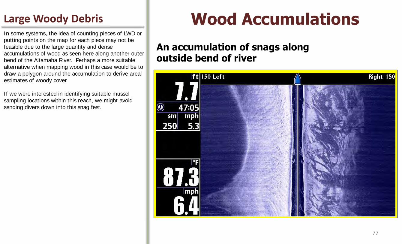
Large Woody Debris Wood Accumulations In some systems, the idea of counting pieces of LWD or putting points on the map for each piece may not be feasible due to the large quantity and dense accumulations of wood as seen here along another outer bend of the Altamaha River. Perhaps a more suitable alternative when mapping wood in this case would be to draw a polygon around the accumulation to derive areal estimates of woody cover. If we were interested in identifying suitable mussel sampling locations within this reach, we might avoid sending divers down into this snag fest.

An accumulation of snags along outside bend of river

77

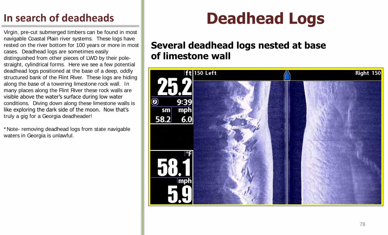
In search of deadheads Deadhead Logs Virgin, pre-cut submerged timbers can be found in most navigable Coastal Plain river systems. These logs have rested on the river bottom for 100 years or more in most cases. Deadhead logs are sometimes easily distinguished from other pieces of LWD by their pole-straight, cylindrical forms. Here we see a few potential deadhead logs positioned at the base of a deep, oddly structured bank of the Flint River. These logs are hiding along the base of a towering limestone rock wall. In many places along the Flint River these rock walls are visible above the water’s surface during low water conditions. Diving down along these limestone walls is like exploring the dark side of the moon. Now that’s truly a gig for a Georgia deadheader! *Note- removing deadhead logs from state navigable waters in Georgia is unlawful.

Several deadhead logs nested at base of limestone wall

78

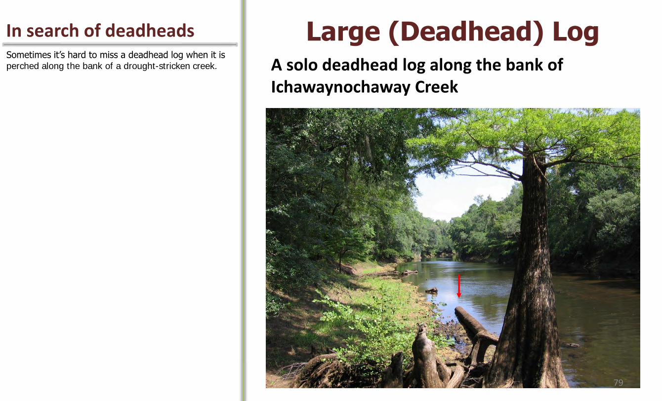
In search of deadheads Large (Deadhead) Log Sometimes it’s hard to miss a deadhead log when it is perched along the bank of a drought-stricken creek. A solo deadhead log along the bank of

Ichawaynochaway Creek

79

In search of deadheads Large (Deadhead) Log Here’s a close-up photo of this same log, with intern Josh Hubbell posing to provide reference on the massive size of this log. The canoe is 16 feet long.

80

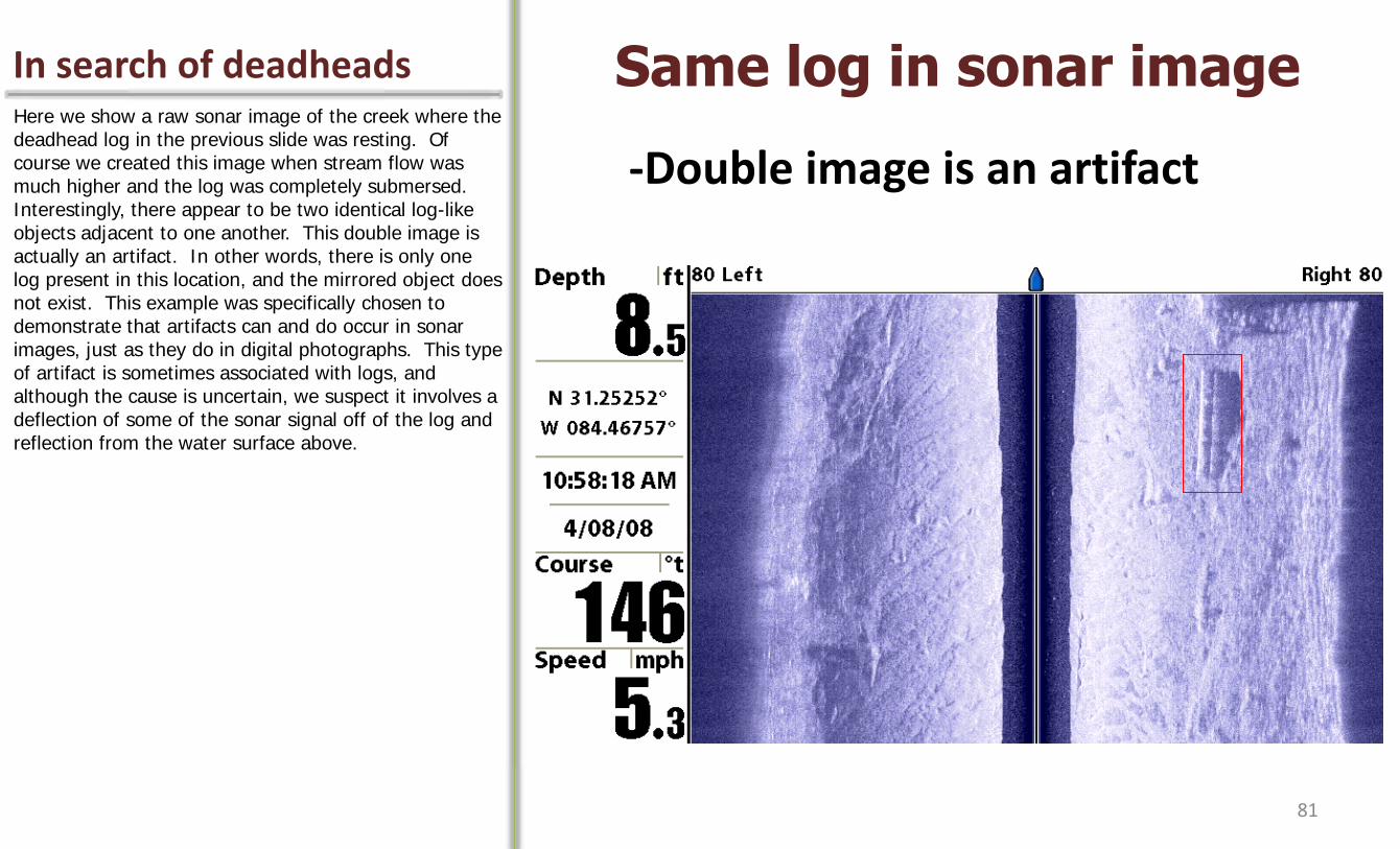
In search of deadheads Same log in sonar image Here we show a raw sonar image of the creek where the deadhead log in the previous slide was resting. Of course we created this image when stream flow was much higher and the log was completely submersed. Interestingly, there appear to be two identical log-like objects adjacent to one another. This double image is actually an artifact. In other words, there is only one log present in this location, and the mirrored object does not exist. This example was specifically chosen to demonstrate that artifacts can and do occur in sonar images, just as they do in digital photographs. This type of artifact is sometimes associated with logs, and although the cause is uncertain, we suspect it involves a deflection of some of the sonar signal off of the log and reflection from the water surface above.

-Double image is an artifact

81

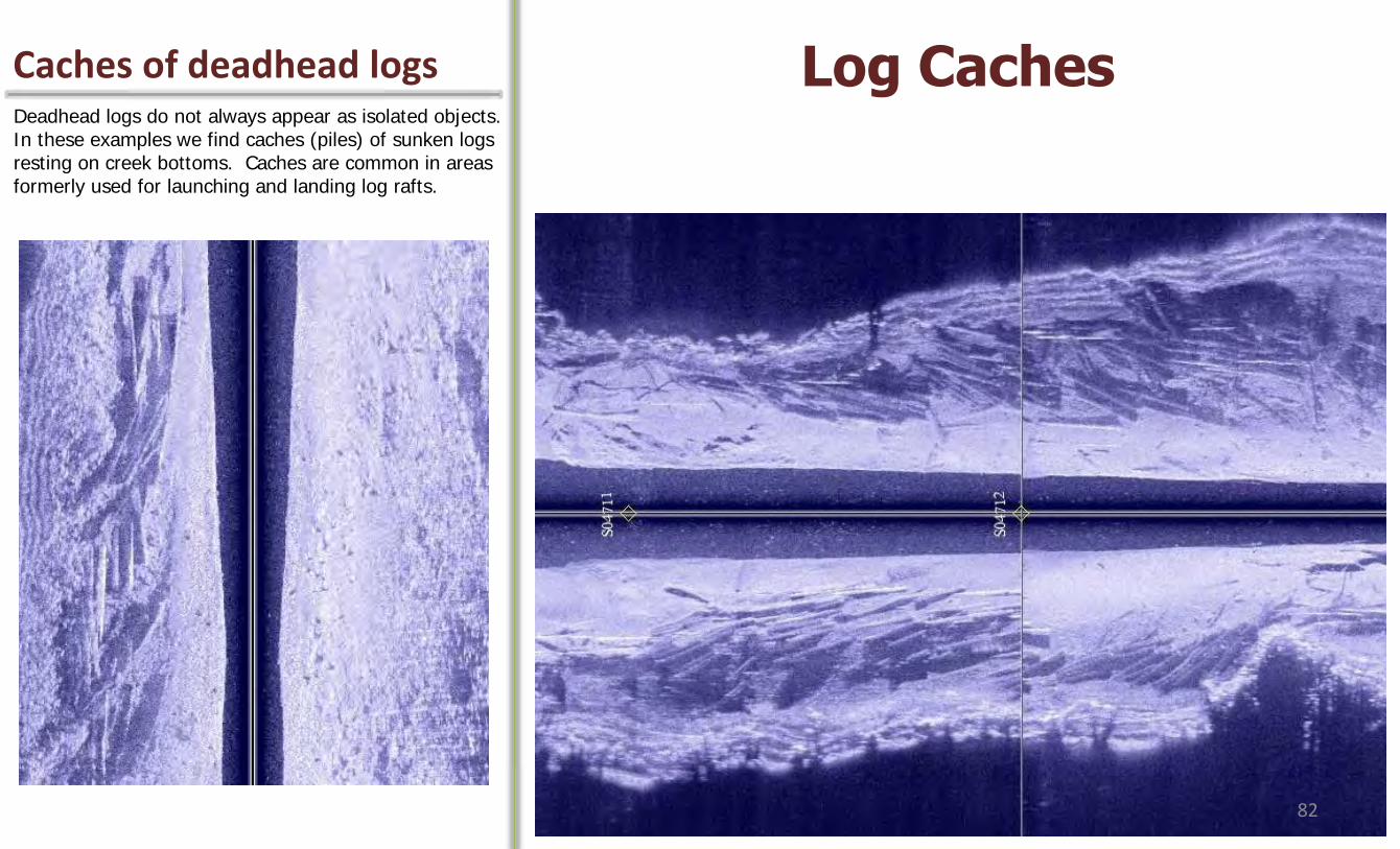
Caches of deadhead logs Log Caches Deadhead logs do not always appear as isolated objects. In these examples we find caches (piles) of sunken logs resting on creek bottoms. Caches are common in areas formerly used for launching and landing log rafts.

82

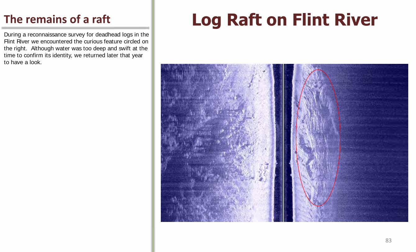
The remains of a raft Log Raft on Flint River During a reconnaissance survey for deadhead logs in the Flint River we encountered the curious feature circled on the right. Although water was too deep and swift at the time to confirm its identity, we returned later that year to have a look.

83

The remains of a raft Log Raft on Flint River What we found during this groundtruthing expedition was a regularly arranged group of logs now exposed along the right bank of the river. Rather than remain preserved underwater, these logs were in various states of decay due to repeated exposure and drying during low flow periods. We suspect this log pile may be the remains of a large log raft that never found its final destination.

84

Features in context Interpreting Features In the following series of slides we will work on interpreting complex features in context. During our early work with sonar mapping we seized the opportunity to visit local creeks during periods of extreme drought and obtain photos, like the one shown here, of study areas. The time spent examining these areas during low, clear water, and the opportunity to study the relationship between field photographs and sonar images of the same areas proved invaluable for honing our skills of interpretation. Let’s spend some time doing the same for a few of these images. In the scene to the right our intern Josh is standing atop a large boulder in the middle of the stream channel, diligently studying the area. To his right an old cypress tree snag stands rooted in the channel. In front of Josh we see another large boulder. Almost touching this boulder is a deadhead log that is oriented parallel to the channel. The topside of this log is just above the water surface. Let’s see if we can pick out each of these objects in the corresponding sonar image.

85 85

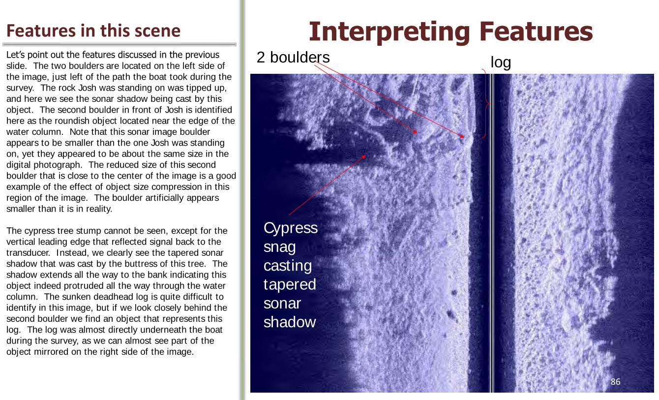
Features in this scene Interpreting Features Let’s point out the features discussed in the previous slide. The two boulders are located on the left side of the image, just left of the path the boat took during the survey. The rock Josh was standing on was tipped up, and here we see the sonar shadow being cast by this object. The second boulder in front of Josh is identified here as the roundish object located near the edge of the water column. Note that this sonar image boulder appears to be smaller than the one Josh was standing on, yet they appeared to be about the same size in the digital photograph. The reduced size of this second boulder that is close to the center of the image is a good example of the effect of object size compression in this region of the image. The boulder artificially appears smaller than it is in reality. The cypress tree stump cannot be seen, except for the vertical leading edge that reflected signal back to the transducer. Instead, we clearly see the tapered sonar shadow that was cast by the buttress of this tree. The shadow extends all the way to the bank indicating this object indeed protruded all the way through the water column. The sunken deadhead log is quite difficult to identify in this image, but if we look closely behind the second boulder we find an object that represents this log. The log was almost directly underneath the boat during the survey, as we can almost see part of the object mirrored on the right side of the image.

Cypress snag casting tapered sonar shadow

2 boulders log

86

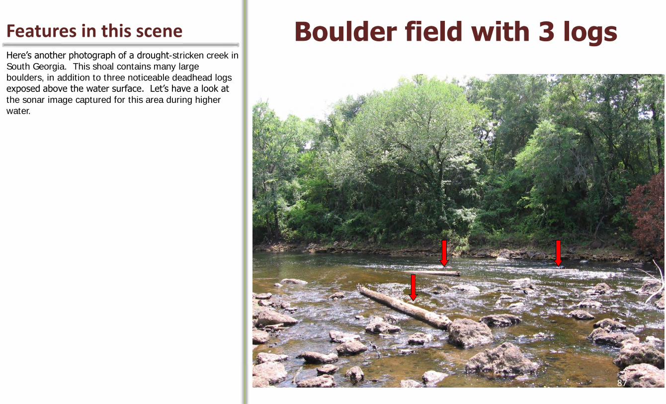
Features in this scene Boulder field with 3 logs Here’s another photograph of a drought-stricken creek in South Georgia. This shoal contains many large boulders, in addition to three noticeable deadhead logs exposed above the water surface. Let’s have a look at the sonar image captured for this area during higher water.

87

Features in this scene Boulder field with 3 logs The field of boulders is quite evident extending across the lower half of this sonar image. Many of these large rocks are casting long shadows, especially because the water was fairly shallow over the shoal during the sonar survey. The three deadhead logs have been identified by red boxes in this image. The survey boat passed over the log in the middle of the image; the log was oriented at an angle to the boat path and as a result we see portions of the log on either side of the image.

88

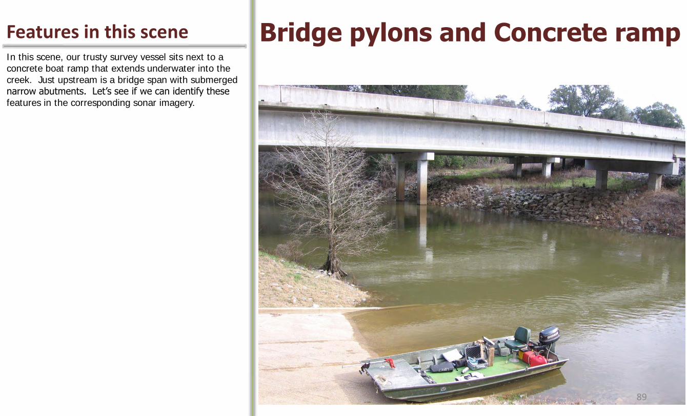
Features in this scene Bridge pylons and Concrete ramp In this scene, our trusty survey vessel sits next to a concrete boat ramp that extends underwater into the creek. Just upstream is a bridge span with submerged narrow abutments. Let’s see if we can identify these features in the corresponding sonar imagery.

89

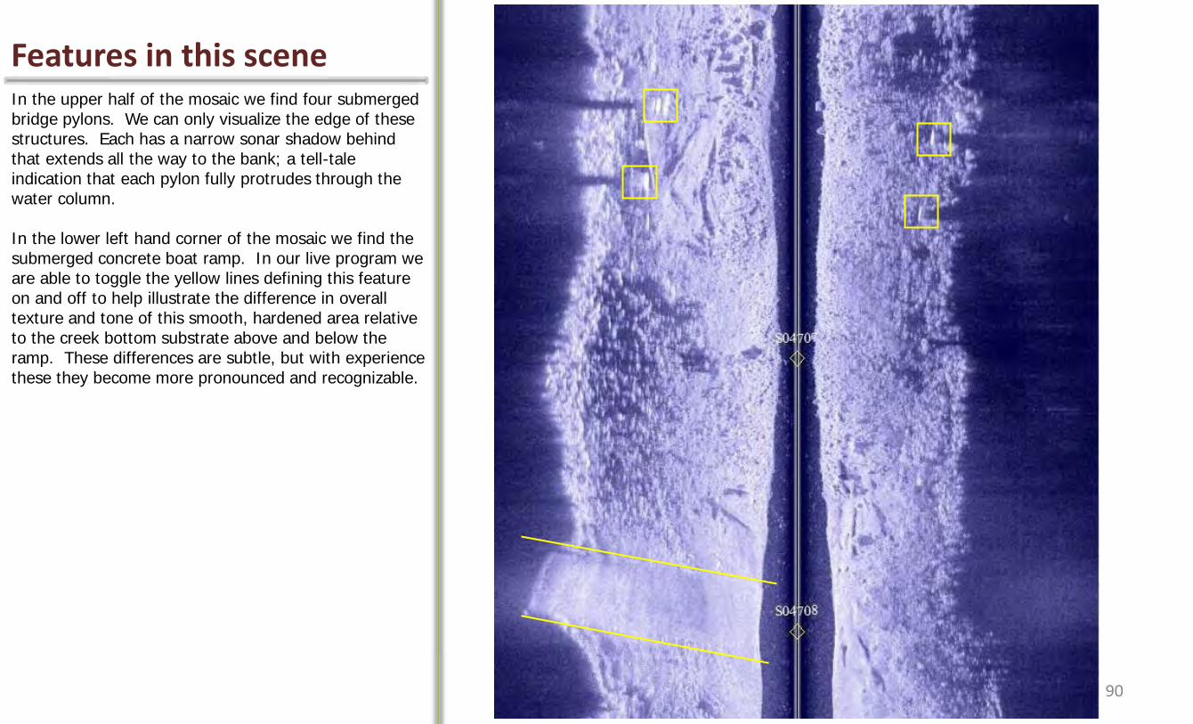
Features in this scene In the upper half of the mosaic we find four submerged bridge pylons. We can only visualize the edge of these structures. Each has a narrow sonar shadow behind that extends all the way to the bank; a tell-tale indication that each pylon fully protrudes through the water column. In the lower left hand corner of the mosaic we find the submerged concrete boat ramp. In our live program we are able to toggle the yellow lines defining this feature on and off to help illustrate the difference in overall texture and tone of this smooth, hardened area relative to the creek bottom substrate above and below the ramp. These differences are subtle, but with experience these they become more pronounced and recognizable.

90

Features in this scene Mid-channel Boulder Shoal In this scene, intern Wes Tracy and I visited an exposed boulder-strewn shoal along Ichawaynochaway Creek for some groundtruth work. The aspect of this photograph reveals how steep the banks of this entrenched creek were in some places. Would you believe we successfully navigated down the center of this creek during a survey? Not at this flow, of course! The yellow line provides an indication of the downstream path taken by our vessel during the sonar survey.

Boat path in sonar image

91

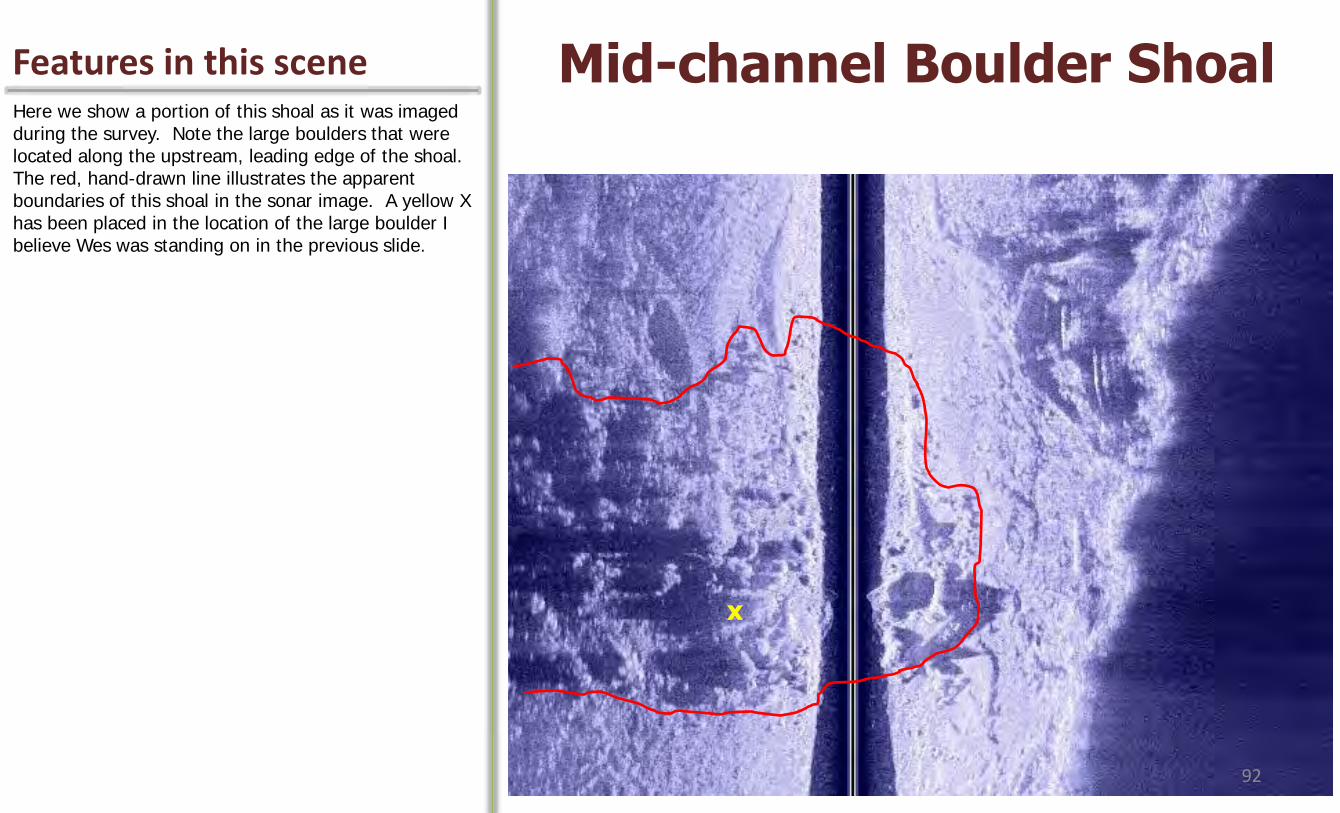
Features in this scene Mid-channel Boulder Shoal Here we show a portion of this shoal as it was imaged during the survey. Note the large boulders that were located along the upstream, leading edge of the shoal. The red, hand-drawn line illustrates the apparent boundaries of this shoal in the sonar image. A yellow X has been placed in the location of the large boulder I believe Wes was standing on in the previous slide.

x

92

A complex scene Pilings, Cypress, and Humps Here is a portion of lower Spring Creek in Southwest Georgia. This area was long ago used as a landing for deadhead logs. A mill and lumber company were located on the adjacent property. Along the far side of the creek we find a series of upright wooden pilings. Note the gap between two adjacent pilings identified with a red line. In the middle of the channel are two small cypress trees identified with red dots. In front of the marked cypress tree closest to the camera is a log oriented perpendicular to the channel (red x). Along the right side of the image (left bank) are two exposed bars or humps. Although it is difficult to tell from this photograph, these bars are actually outcrops of solid limestone bedrock. The surrounding substrate was mud and silt.

X

93

Features in this scene Here we display this reach of the creek in raw sonar image mosaic form. On the left is the raw mosaic, and on the right we have added reference markers for the features identified in the previous slide. Notice how each upright piling casts a long narrow shadow that reaches the right bank. The gap between the two pilings is clearly evident. It is somewhat difficult to identify the two upright cypress trees because each was rooted on a raised portion of the bed. The approximate positions of these trees have been identified with red circles. And lastly, the two limestone outcrops have been identified with the shaded polygons on the right hand mosaic. The difference in texture between these outcrops and the surrounding muddy substrate are quite subtle. Interpreting these substrate distinctions is challenging in this scene.

94

A popular question Can fish be seen? The question of whether fish can be imaged by side scan sonar is relevant and intriguing. Until now we have focused on inert physical features and objects, yet all of the streams we have scanned have resident fish populations. What does it take to image a fish? Several important factors having to do with operation of the sonar equipment, such as the range setting used, will likely play a role in imaging fish. At higher range settings, smaller objects (fish) are less likely to appear as distinguishable targets in an image. As far as subjects go, fish that are larger and more reflective (hard-bodied) like the Gulf sturgeon to the right, probably stand a better chance of being imaged by side scan sonar. Fish with soft bodies, like catfish, may absorb too much of the sonar signal to be detected, although much work remains to explore differences among fishes. At least one study demonstrating the use of the Humminbird system for detecting manatees (see reference below) appears in the primary literature, and others are underway examining the effectiveness of detecting and counting sturgeon with side scan sonar.

Gulf sturgeon: a large, reflective target

Gonzalez-Socoloske, D., L. D. Olivera-Gomez, and R. E. Ford. 2009. Detection of free-ranging West Indian manatees Trichechus manatus using side-scan sonar. Endangered Species Research, 8: 249-257.

95

Sturgeon in resting area Gulf Sturgeon Here is a single image captured in a known resting area for Gulf sturgeon that typically holds dozens if not hundreds of sturgeon. Many of the suspended targets seen here are likely sturgeon. Below we zoom in on the target just right of center to examine its shadow profile. Note the sloping forehead, heterocercal tail, pectoral and pelvic fins. Interestingly, it is the shadow of sturgeon rather than the target itself that often appears so well defined in the sonar image.

96

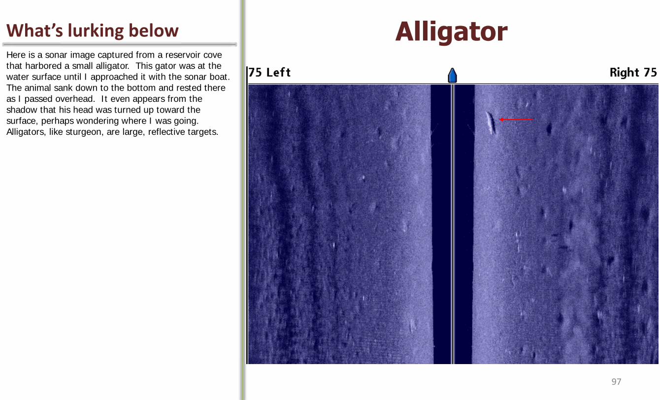
What’s lurking below Alligator Here is a sonar image captured from a reservoir cove that harbored a small alligator. This gator was at the water surface until I approached it with the sonar boat. The animal sank down to the bottom and rested there as I passed overhead. It even appears from the shadow that his head was turned up toward the surface, perhaps wondering where I was going. Alligators, like sturgeon, are large, reflective targets.

97

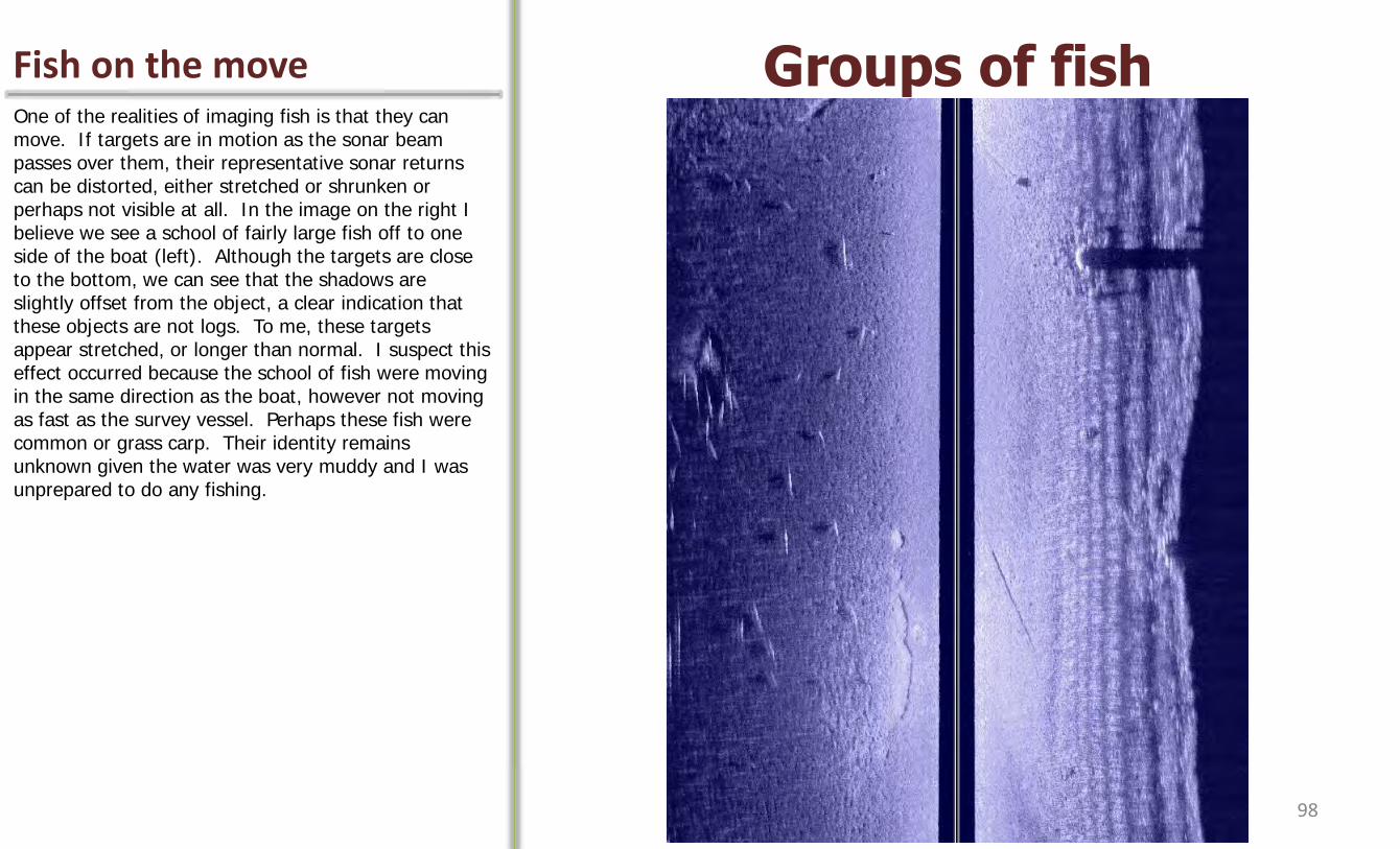
Fish on the move Groups of fish One of the realities of imaging fish is that they can move. If targets are in motion as the sonar beam passes over them, their representative sonar returns can be distorted, either stretched or shrunken or perhaps not visible at all. In the image on the right I believe we see a school of fairly large fish off to one side of the boat (left). Although the targets are close to the bottom, we can see that the shadows are slightly offset from the object, a clear indication that these objects are not logs. To me, these targets appear stretched, or longer than normal. I suspect this effect occurred because the school of fish were moving in the same direction as the boat, however not moving as fast as the survey vessel. Perhaps these fish were common or grass carp. Their identity remains unknown given the water was very muddy and I was unprepared to do any fishing.

98

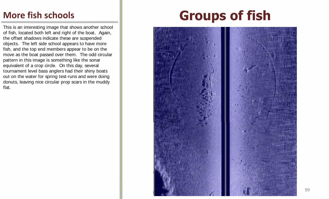
More fish schools Groups of fish This is an interesting image that shows another school of fish, located both left and right of the boat. Again, the offset shadows indicate these are suspended objects. The left side school appears to have more fish, and the top end members appear to be on the move as the boat passed over them. The odd circular pattern in this image is something like the sonar equivalent of a crop circle. On this day, several tournament level bass anglers had their shiny boats out on the water for spring test-runs and were doing donuts, leaving nice circular prop scars in the muddy flat.

99

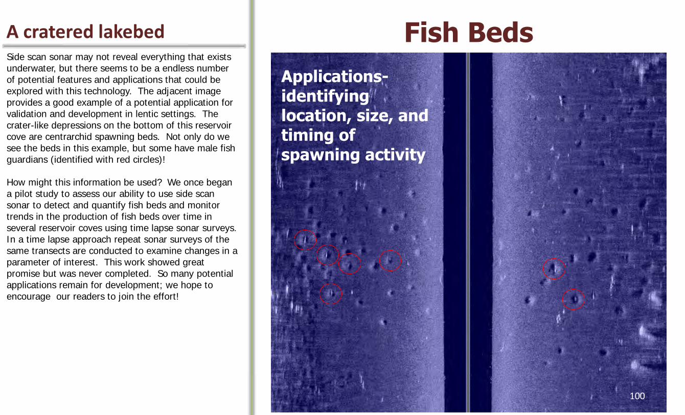
A cratered lakebed Fish Beds Side scan sonar may not reveal everything that exists underwater, but there seems to be a endless number of potential features and applications that could be explored with this technology. The adjacent image provides a good example of a potential application for validation and development in lentic settings. The crater-like depressions on the bottom of this reservoir cove are centrarchid spawning beds. Not only do we see the beds in this example, but some have male fish guardians (identified with red circles)! How might this information be used? We once began a pilot study to assess our ability to use side scan sonar to detect and quantify fish beds and monitor trends in the production of fish beds over time in several reservoir coves using time lapse sonar surveys. In a time lapse approach repeat sonar surveys of the same transects are conducted to examine changes in a parameter of interest. This work showed great promise but was never completed. So many potential applications remain for development; we hope to encourage our readers to join the effort!

Applications- identifying location, size, and timing of spawning activity

100

A cratered lakebed Colonial bed formations Here are a few other images showing bed aggregations along reservoir shorelines. Unlike the scattered beds in the previous slide these are very tightly spaced, suggesting colonial spawning aggregations of bream.

29 m2

76 m2

25 m2

101

What about plants? Submerged Aquatic Vegetation In every workshop we’ve ever hosted, someone has asked about aquatic vegetation. Does sonar reveal submerged aquatic vegetation and what applications exist for the study of SAV with side scan sonar? Our experience with SAV is limited, having worked primarily in streams where vegetation does not exist. However, when taking sonar into reservoirs and lakes we have captured images like this one. Here, we navigated our sonar boat over a vast bed of hydrilla, a troublesome invasive plant that forms thick colonies in shallow waters. The stems of this plant can grow to reach the water surface, and in doing so these plants block and reflect much of the sonar signal as shown here. This hydrilla bed appears to have a sonar signature unlike any of the “substrates” previously examined in this chapter. If other types of SAV also provide unique or distinguishable sonar signatures in imagery, then the idea of mapping and monitoring SAV with side scan sonar has great promise, and should be investigated.

Plant growth through water column to surface will reflect (block) sound

102

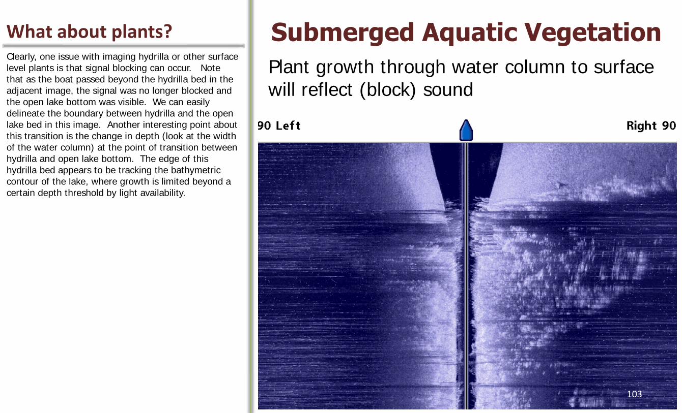
What about plants? Submerged Aquatic Vegetation Clearly, one issue with imaging hydrilla or other surface level plants is that signal blocking can occur. Note that as the boat passed beyond the hydrilla bed in the adjacent image, the signal was no longer blocked and the open lake bottom was visible. We can easily delineate the boundary between hydrilla and the open lake bed in this image. Another interesting point about this transition is the change in depth (look at the width of the water column) at the point of transition between hydrilla and open lake bottom. The edge of this hydrilla bed appears to be tracking the bathymetric contour of the lake, where growth is limited beyond a certain depth threshold by light availability.

Plant growth through water column to surface will reflect (block) sound

103

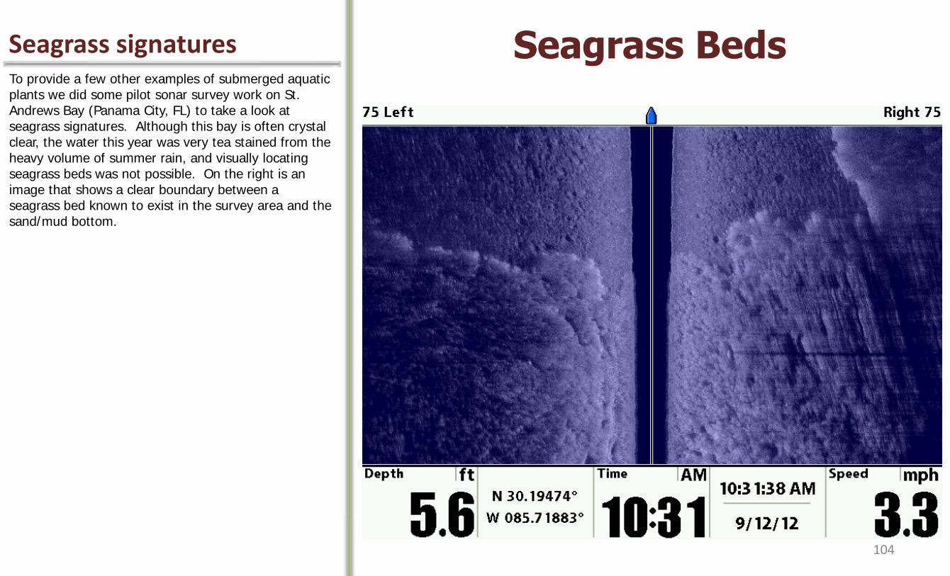
Seagrass signatures Seagrass Beds To provide a few other examples of submerged aquatic plants we did some pilot sonar survey work on St. Andrews Bay (Panama City, FL) to take a look at seagrass signatures. Although this bay is often crystal clear, the water this year was very tea stained from the heavy volume of summer rain, and visually locating seagrass beds was not possible. On the right is an image that shows a clear boundary between a seagrass bed known to exist in the survey area and the sand/mud bottom.

104

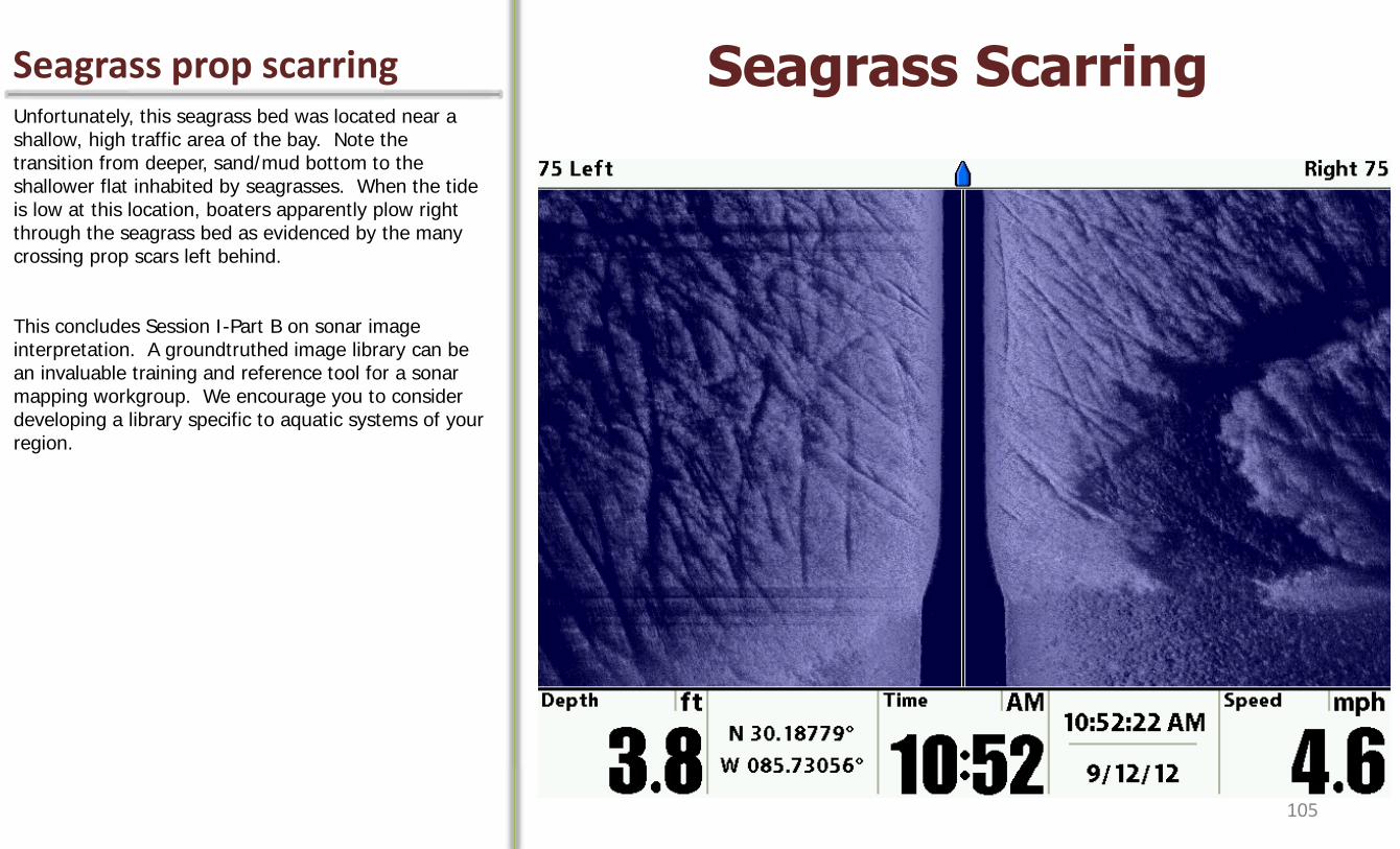
Seagrass prop scarring Seagrass Scarring Unfortunately, this seagrass bed was located near a shallow, high traffic area of the bay. Note the transition from deeper, sand/mud bottom to the shallower flat inhabited by seagrasses. When the tide is low at this location, boaters apparently plow right through the seagrass bed as evidenced by the many crossing prop scars left behind. This concludes Session I-Part B on sonar image interpretation. A groundtruthed image library can be an invaluable training and reference tool for a sonar mapping workgroup. We encourage you to consider developing a library specific to aquatic systems of your region.

105

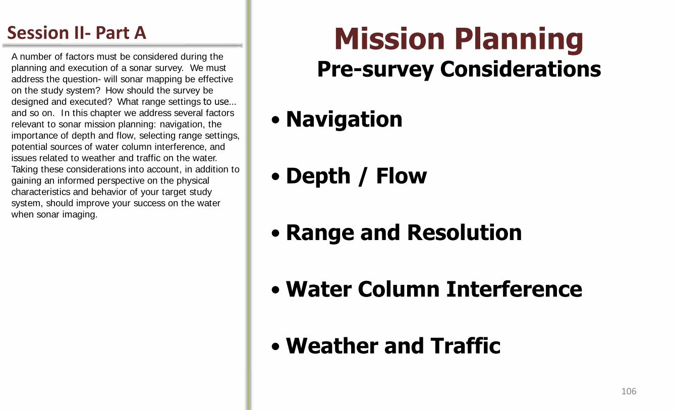
Session II- Part A Mission Planning Pre-survey Considerations

• Navigation

• Depth / Flow

• Range and Resolution

• Water Column Interference

• Weather and Traffic

A number of factors must be considered during the planning and execution of a sonar survey. We must address the question- will sonar mapping be effective on the study system? How should the survey be designed and executed? What range settings to use… and so on. In this chapter we address several factors relevant to sonar mission planning: navigation, the importance of depth and flow, selecting range settings, potential sources of water column interference, and issues related to weather and traffic on the water. Taking these considerations into account, in addition to gaining an informed perspective on the physical characteristics and behavior of your target study system, should improve your success on the water when sonar imaging.

106

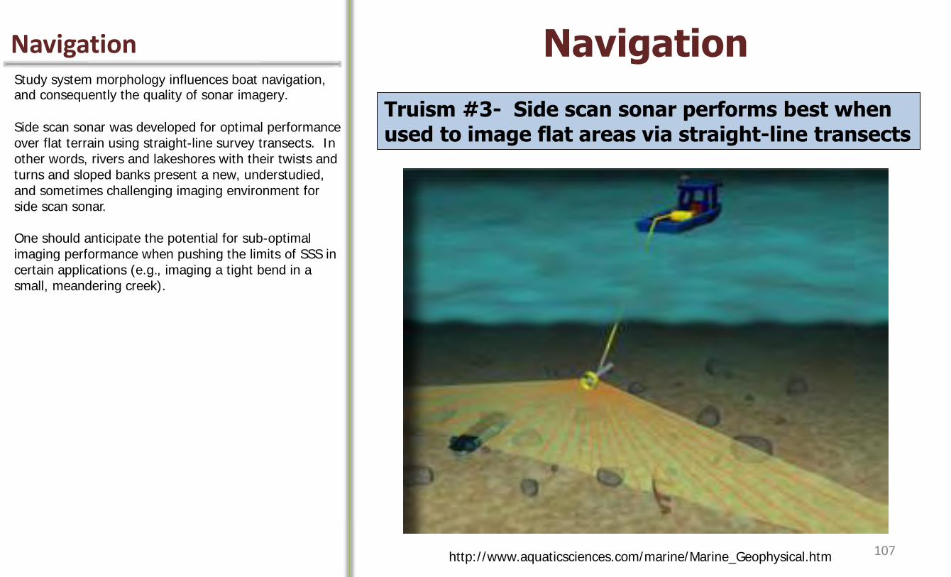
Navigation Navigation

http://www.aquaticsciences.com/marine/Marine_Geophysical.htm

Truism #3- Side scan sonar performs best when used to image flat areas via straight-line transects

Study system morphology influences boat navigation, and consequently the quality of sonar imagery. Side scan sonar was developed for optimal performance over flat terrain using straight-line survey transects. In other words, rivers and lakeshores with their twists and turns and sloped banks present a new, understudied, and sometimes challenging imaging environment for side scan sonar. One should anticipate the potential for sub-optimal imaging performance when pushing the limits of SSS in certain applications (e.g., imaging a tight bend in a small, meandering creek).

107

Boat Navigation Navigation Issues During navigation of sinuous transects, the sonar signal may overlap on the inside of a turn, and fan out along the outside of a turn potentially causing distortion and data gaps in sonar imagery. The degree of overlap or fanning (and hence distortion) will depend on several factors, including the radius of the turn, the range setting used, the pulse rate, and boat speed. The best performance of SSS will be achieved during straight line navigation and gradual turning when necessary.

overlapping

fanning

108

Effect of sharp turns Chickasawhatchee Creek To illustrate the effect of navigation-induced image distortion, we captured imagery during navigation of two available routes around a small island in a reach of Chickasawhatchee Creek in Southwest Georgia. Heavy shoals (rocky areas) were located on the inside route. Both routes required evasive maneuvering to avoid disaster.

Narrow & sinuous channels could pose the following problems:

• Image distortion in bends due to pulse overlap

• Poor GPS accuracy under thick canopy

109

The Inside Bend Navigating Sharp Bends Navigating the inside route demanded a sharp turn to the left (port) as we approached the island (located approximately at the head of the red arrow on the raw sonar mosaic). Note the “stretch” distortion that occurred as a result of sonar beams overlapping back over previously insonified (i.e., scanned) areas. Just below the heavy shoal, the image appears somewhat hazy or milky in appearance- this is the effect of water column turbulence created by the rocky shoal. Note, too, that the island effectively blocks the sonar signal from reaching habitat on the far side of the channel.

110

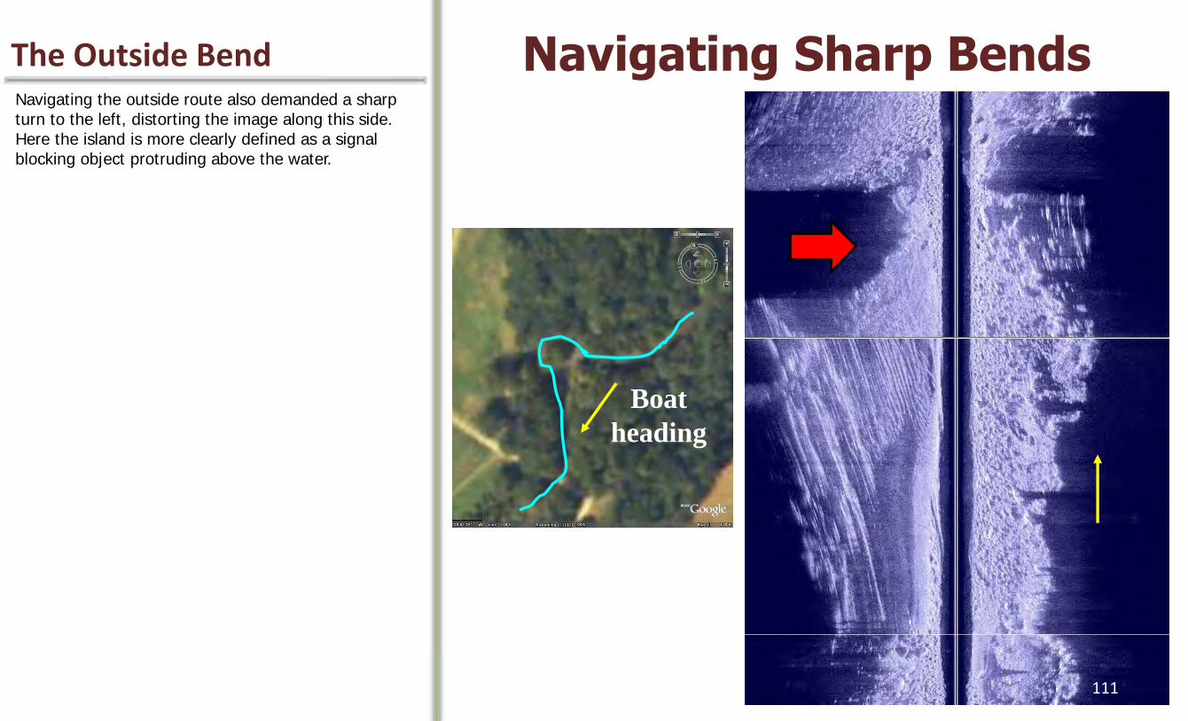
The Outside Bend Navigating Sharp Bends Navigating the outside route also demanded a sharp turn to the left, distorting the image along this side. Here the island is more clearly defined as a signal blocking object protruding above the water.

Boat

heading

111

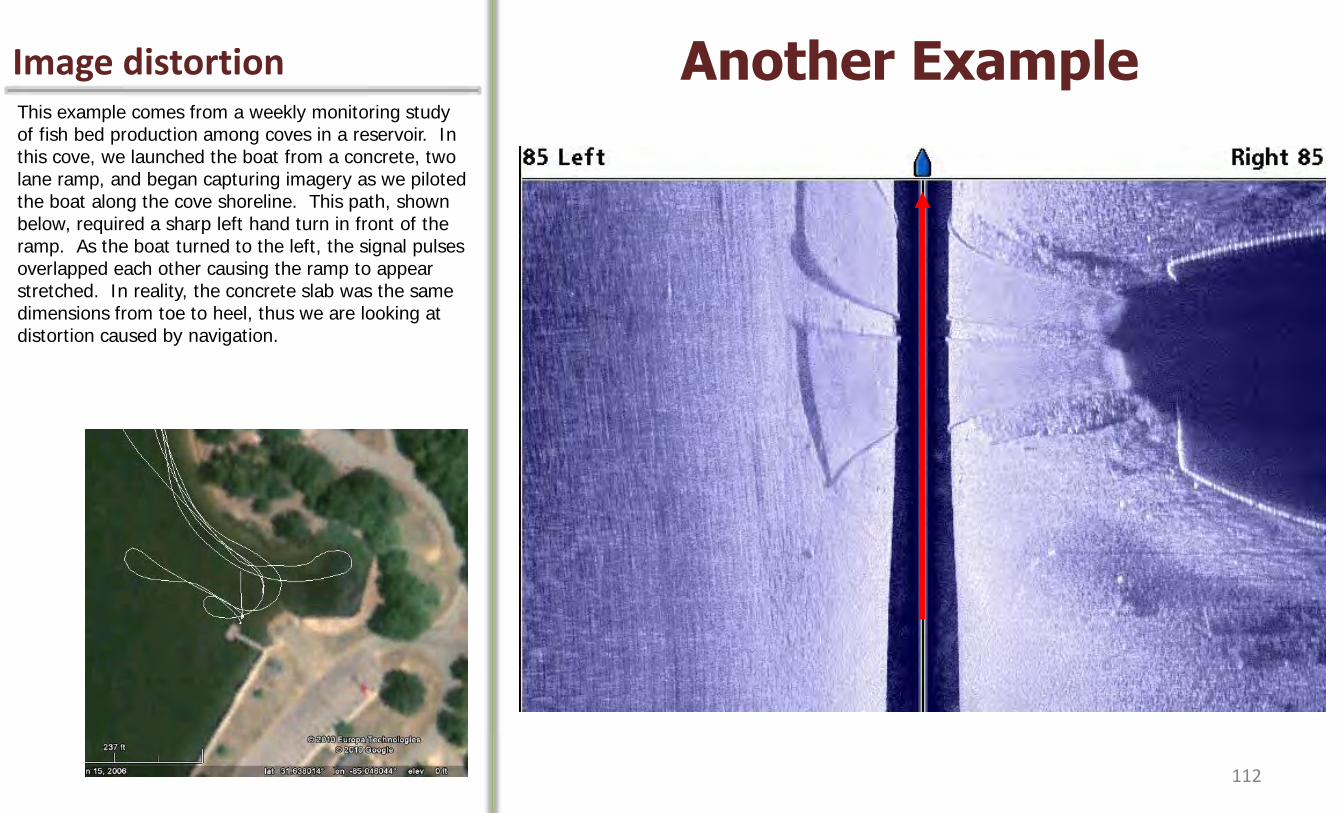
Image distortion Another Example This example comes from a weekly monitoring study of fish bed production among coves in a reservoir. In this cove, we launched the boat from a concrete, two lane ramp, and began capturing imagery as we piloted the boat along the cove shoreline. This path, shown below, required a sharp left hand turn in front of the ramp. As the boat turned to the left, the signal pulses overlapped each other causing the ramp to appear stretched. In reality, the concrete slab was the same dimensions from toe to heel, thus we are looking at distortion caused by navigation.

112

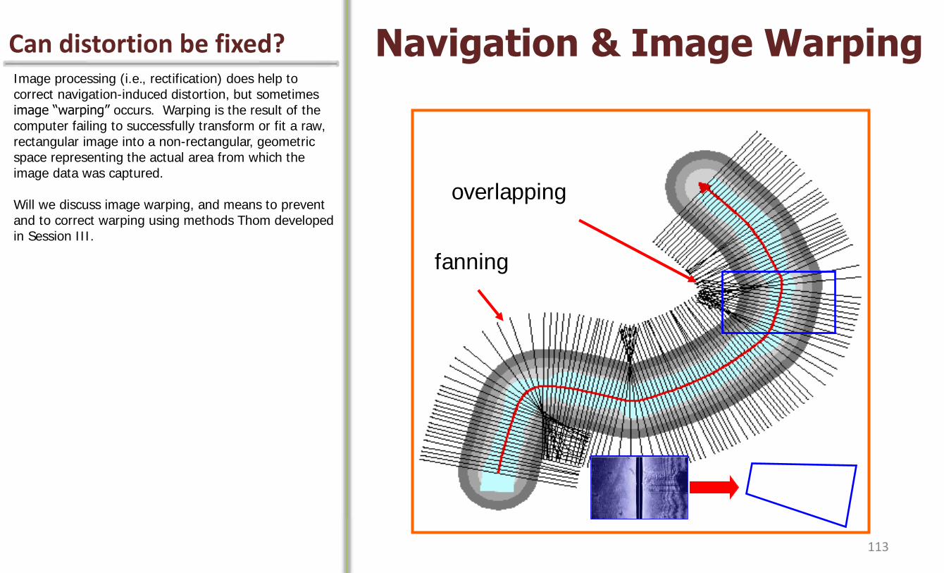
Can distortion be fixed? Navigation & Image Warping Image processing (i.e., rectification) does help to correct navigation-induced distortion, but sometimes image “warping” occurs. Warping is the result of the computer failing to successfully transform or fit a raw, rectangular image into a non-rectangular, geometric space representing the actual area from which the image data was captured. Will we discuss image warping, and means to prevent and to correct warping using methods Thom developed in Session III.

overlapping

fanning

113

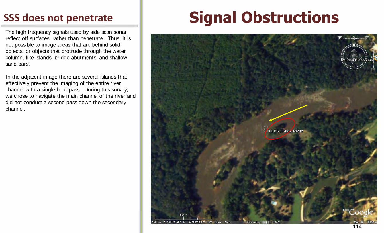
SSS does not penetrate Signal Obstructions The high frequency signals used by side scan sonar reflect off surfaces, rather than penetrate. Thus, it is not possible to image areas that are behind solid objects, or objects that protrude through the water column, like islands, bridge abutments, and shallow sand bars. In the adjacent image there are several islands that effectively prevent the imaging of the entire river channel with a single boat pass. During this survey, we chose to navigate the main channel of the river and did not conduct a second pass down the secondary channel.

114

SSS does not penetrate Signal Obstructions The island appears on the left side of this raw image mosaic. The outer edge of the island is clearly defined, however, the secondary channel behind this island is not imaged, and represents missing data. Note too that a large boulder shoal occupied the main river channel adjacent to this island. Higher flows on the day of the survey allowed us to navigate over this shoal, even though the river was shallow in places along the boat path. Very shallow portions of the shoal that contained large protruding boulders cast areas of “sonar shadow”. Areas obscured by sonar shadow also represent missing data. If the river discharge and stage were higher during the survey, the extent of the sonar shadowed areas would likely have been reduced. The opposite is also true, of course. If river stage was lower, more areas in this image may have been covered by sonar shadows.

Island

Shoal

115

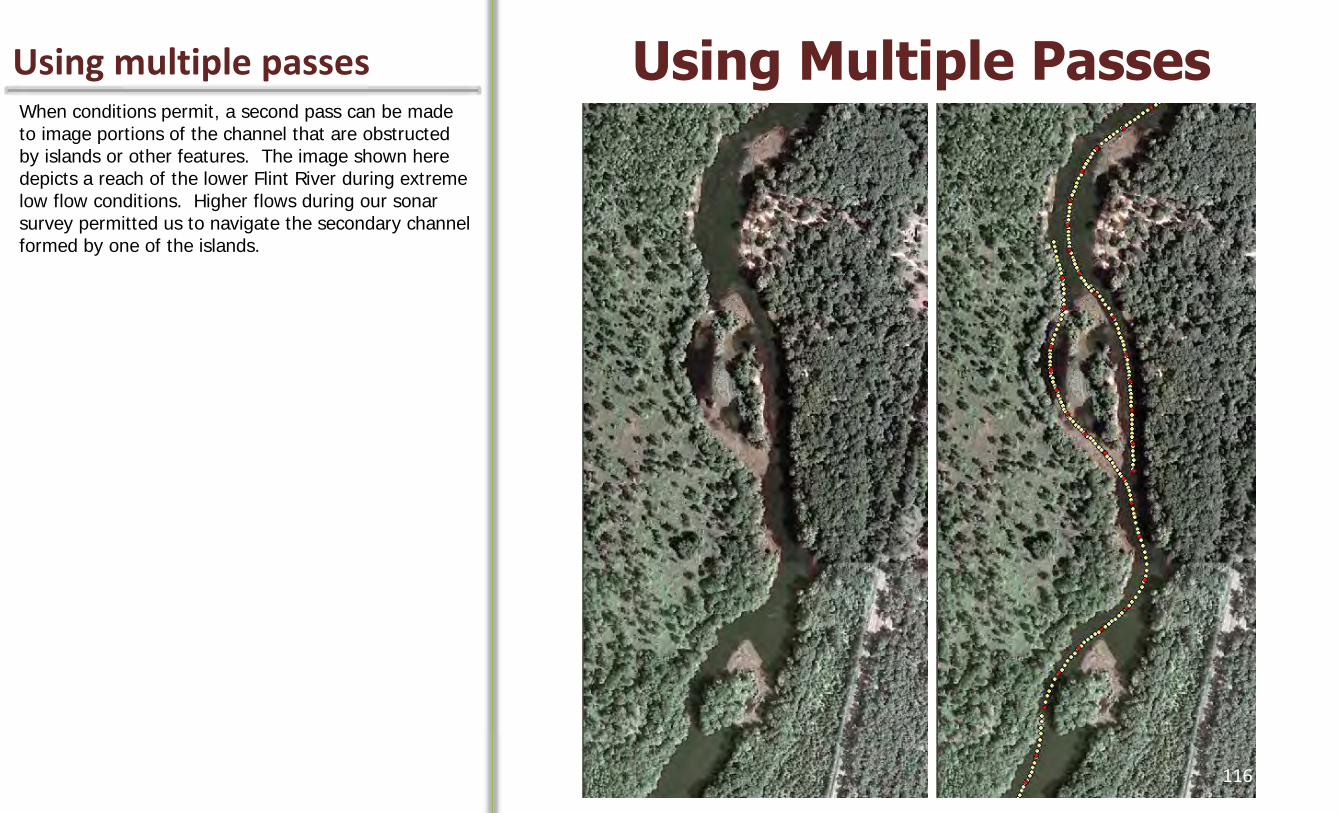
Using Multiple Passes When conditions permit, a second pass can be made to image portions of the channel that are obstructed by islands or other features. The image shown here depicts a reach of the lower Flint River during extreme low flow conditions. Higher flows during our sonar survey permitted us to navigate the secondary channel formed by one of the islands.

Using multiple passes

116

Using Multiple Passes Imagery captured during the two passes will ultimately be processed as two separate survey segments, and the rectified sonar image map layers can be displayed in a GIS as overlays. When interpreting and digitizing habitat features from overlapping image layers, it is possible to make one semi-transparent, to toggle the overlapping layers on and off, or simply move the better of the two layers to the top to facilitate interpretation of features in overlapping portions of the mosaic.


117

Using Multiple Passes Once digitization and classification is complete, the classified substrate layer can be displayed and the sonar image layers removed. Here we see digitized polygons representing each substrate class in the classification scheme. Polygons representing the two islands, areas that were hidden by sonar shadow (black polygons), and areas not imaged because they were beyond sonar range (red polygons) are also represented in this map layer.


118

How shallow? Minimum System Depth What is the minimum depth at which surveys can be conducted? Obviously, enough water must be present to permit unimpeded navigation using some mechanism for forward propulsion.

• Limited by depth required for navigation

…but surveys do not necessarily require a johnboat

• Other possibilities- gheenoe, kayak?

119

Johnboat with 30 HP motor Survey Watercraft In flowing waters, a source of propulsion (thrust) is necessary to maintain heading, position, and speed. Propulsion is also essential to avoid the many dangers lurking beneath murky waters. This 14-foot, lightweight johnboat proved to be very effective for sonar mapping in most of the creeks and rivers of Southwest Georgia. With the use of a roller trailer (trailer with rolling supports) it was possible for one person to launch this boat off a steep bank, whenever ramps were unavailable. I found the flat bottom of this boat ideal for stability on the water, a feature that supports the production of high quality imagery. As you can see, it doesn’t take much boat to get the job done. The control head is close at hand should the order to abandon ship be delivered. *The position of the transducer is somewhat misleading in this photograph. It appears to be only and inch or two below the waters surface. In reality, I had a crew member on board who sat in front of this boat, adding weight and stability to the bow, ensuring that the transducer was actually deployed about 6 inches below the surface. This crew member was left on the bank to take this picture.

Control Head

Transducer

GPS Receiver

120

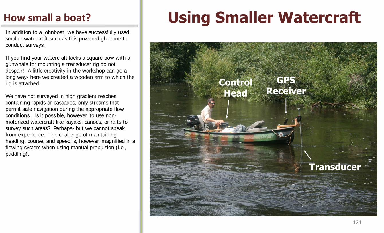
How small a boat? Using Smaller Watercraft In addition to a johnboat, we have successfully used smaller watercraft such as this powered gheenoe to conduct surveys. If you find your watercraft lacks a square bow with a gunwhale for mounting a transducer rig do not despair! A little creativity in the workshop can go a long way- here we created a wooden arm to which the rig is attached. We have not surveyed in high gradient reaches containing rapids or cascades, only streams that permit safe navigation during the appropriate flow conditions. Is it possible, however, to use non-motorized watercraft like kayaks, canoes, or rafts to survey such areas? Perhaps- but we cannot speak from experience. The challenge of maintaining heading, course, and speed is, however, magnified in a flowing system when using manual propulsion (i.e., paddling).

GPS Receiver

Transducer

Control Head

121

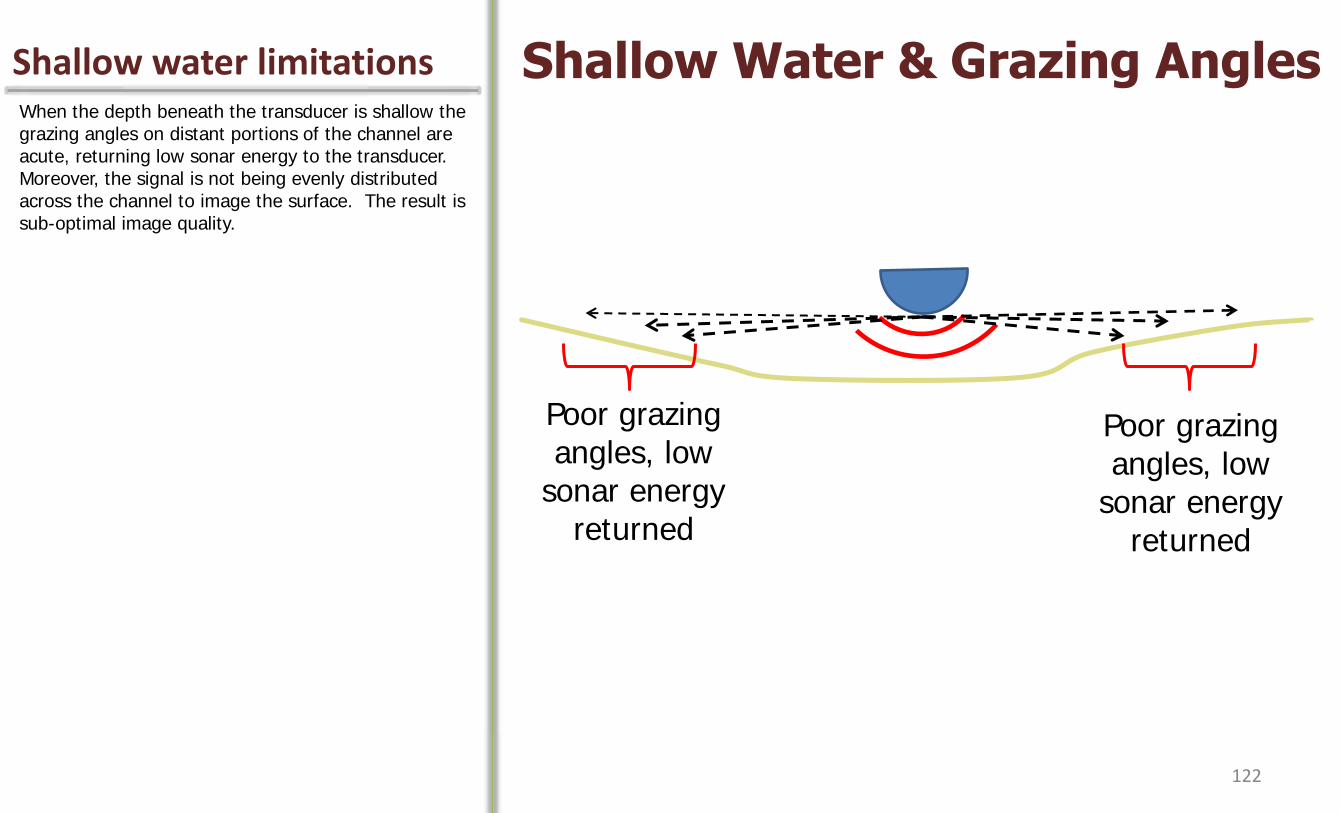
Shallow water limitations Shallow Water & Grazing Angles When the depth beneath the transducer is shallow the grazing angles on distant portions of the channel are acute, returning low sonar energy to the transducer. Moreover, the signal is not being evenly distributed across the channel to image the surface. The result is sub-optimal image quality.

GPS Receiver

Transducer

Control Head

Poor grazing angles, low

sonar energy returned

Poor grazing angles, low

sonar energy returned

122

Shallow water limitations Shallow Water Example Very shallow water typically hinders effective imaging of the entire channel. Although water depth along the boat track was <3 feet in this example, slightly deeper water was found to the right of the boat, and this part of the channel was imaged. To the left of the image we cannot see the actual river bank; a shallow sandbar occupied this area of the river channel. Notice the dark streaks along the left near the boat path. Any guess as to what caused these features? I wasn’t the only one having difficulty navigating through this flat. It is interesting to note that the channel, or deepest water, appears to be on the far right hand side of the image, along the bank. The shadow cast by the sandbar suggests a drop off, or slightly deeper channel along the river margin.

123

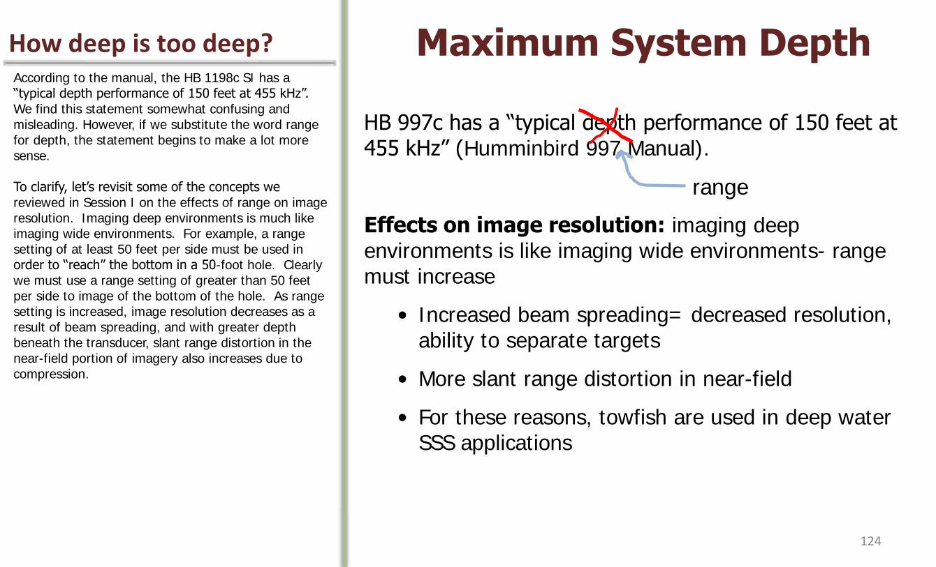
How deep is too deep? Maximum System Depth According to the manual, the HB 1198c SI has a “typical depth performance of 150 feet at 455 kHz”. We find this statement somewhat confusing and misleading. However, if we substitute the word range for depth, the statement begins to make a lot more sense. To clarify, let’s revisit some of the concepts we reviewed in Session I on the effects of range on image resolution. Imaging deep environments is much like imaging wide environments. For example, a range setting of at least 50 feet per side must be used in order to “reach” the bottom in a 50-foot hole. Clearly we must use a range setting of greater than 50 feet per side to image of the bottom of the hole. As range setting is increased, image resolution decreases as a result of beam spreading, and with greater depth beneath the transducer, slant range distortion in the near-field portion of imagery also increases due to compression.

HB 997c has a “typical depth performance of 150 feet at 455 kHz” (Humminbird 997 Manual).

Effects on image resolution: imaging deep environments is like imaging wide environments- range must increase

• Increased beam spreading= decreased resolution, ability to separate targets

• More slant range distortion in near-field

• For these reasons, towfish are used in deep water SSS applications

range

124

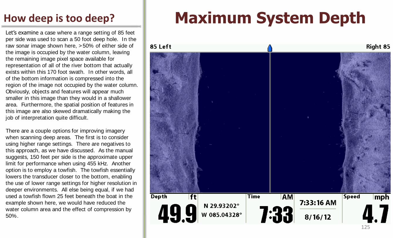
How deep is too deep? Maximum System Depth Let’s examine a case where a range setting of 85 feet per side was used to scan a 50 foot deep hole. In the raw sonar image shown here, >50% of either side of the image is occupied by the water column, leaving the remaining image pixel space available for representation of all of the river bottom that actually exists within this 170 foot swath. In other words, all of the bottom information is compressed into the region of the image not occupied by the water column. Obviously, objects and features will appear much smaller in this image than they would in a shallower area. Furthermore, the spatial position of features in this image are also skewed dramatically making the job of interpretation quite difficult. There are a couple options for improving imagery when scanning deep areas. The first is to consider using higher range settings. There are negatives to this approach, as we have discussed. As the manual suggests, 150 feet per side is the approximate upper limit for performance when using 455 kHz. Another option is to employ a towfish. The towfish essentially lowers the transducer closer to the bottom, enabling the use of lower range settings for higher resolution in deeper environments. All else being equal, if we had used a towfish flown 25 feet beneath the boat in the example shown here, we would have reduced the water column area and the effect of compression by 50%.

125

Information available Towfish for Humminbird SI? If interested in purchasing or building a towfish for the Humminbird system, you may find useful information on the internet at the side imaging forums. The photos of towfish shown here were obtained from these websites. The “tank” was a for-sale towfish, and the yellow fish was homemade. Humminbird sells an extension cable to lengthen the line between the control head and the transducer. We do not have experience working with the Humminbird system and a towfish, mostly because our survey systems are generally not deep enough to warrant this type of deployment.

“the Tank”

Humminbird Side Imaging Forums

http://forums.sideimagingsoft.com/index.php

http://www.xumba.scholleco.com/

126

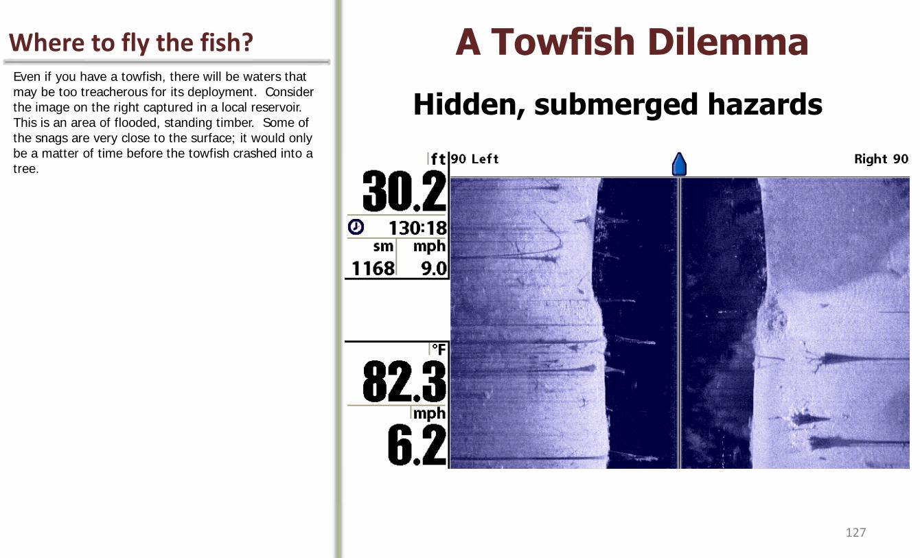
Where to fly the fish? A Towfish Dilemma Even if you have a towfish, there will be waters that may be too treacherous for its deployment. Consider the image on the right captured in a local reservoir. This is an area of flooded, standing timber. Some of the snags are very close to the surface; it would only be a matter of time before the towfish crashed into a tree.

Hidden, submerged hazards

127

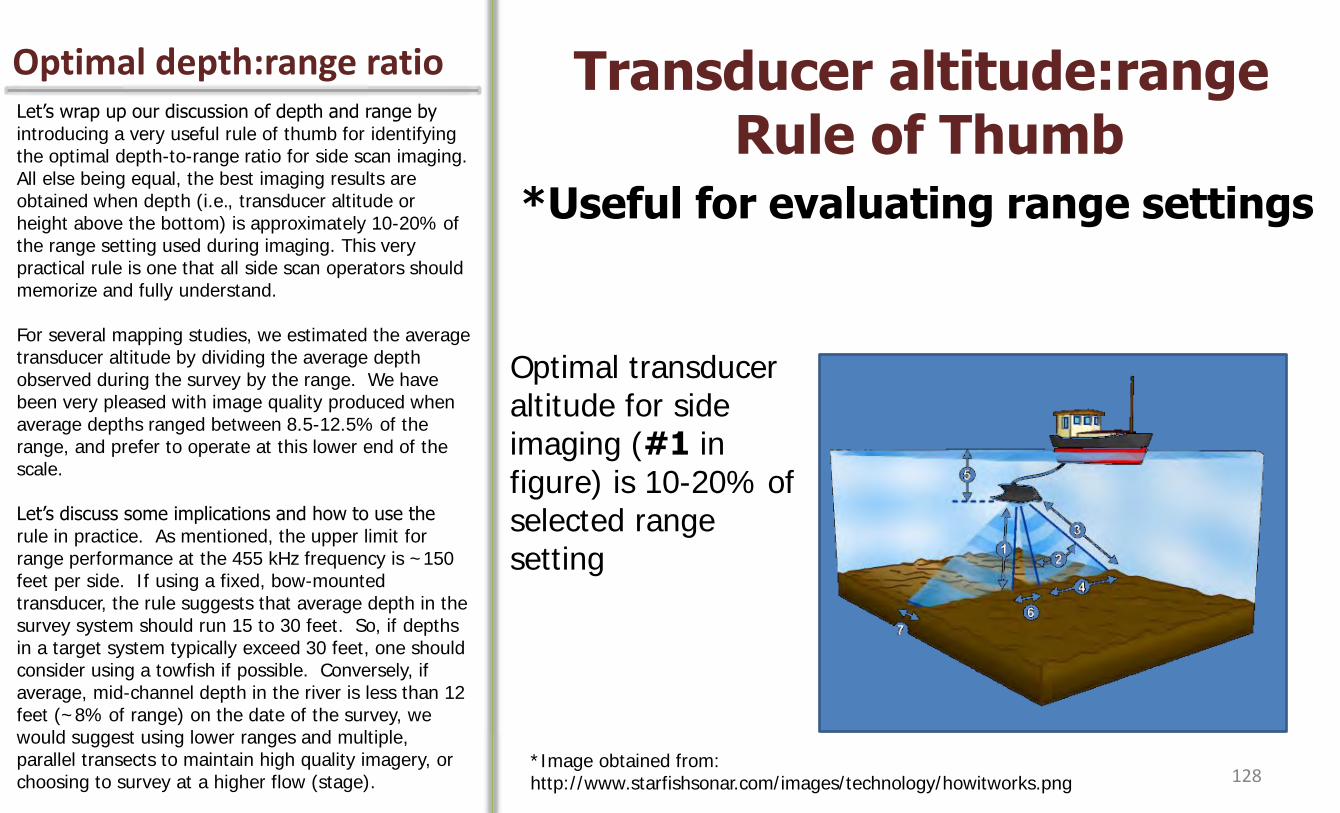
Optimal depth:range ratio Transducer altitude:range Rule of Thumb

Let’s wrap up our discussion of depth and range by introducing a very useful rule of thumb for identifying the optimal depth-to-range ratio for side scan imaging. All else being equal, the best imaging results are obtained when depth (i.e., transducer altitude or height above the bottom) is approximately 10-20% of the range setting used during imaging. This very practical rule is one that all side scan operators should memorize and fully understand. For several mapping studies, we estimated the average transducer altitude by dividing the average depth observed during the survey by the range. We have been very pleased with image quality produced when average depths ranged between 8.5-12.5% of the range, and prefer to operate at this lower end of the scale. Let’s discuss some implications and how to use the rule in practice. As mentioned, the upper limit for range performance at the 455 kHz frequency is ~150 feet per side. If using a fixed, bow-mounted transducer, the rule suggests that average depth in the survey system should run 15 to 30 feet. So, if depths in a target system typically exceed 30 feet, one should consider using a towfish if possible. Conversely, if average, mid-channel depth in the river is less than 12 feet (~8% of range) on the date of the survey, we would suggest using lower ranges and multiple, parallel transects to maintain high quality imagery, or choosing to survey at a higher flow (stage).

*Useful for evaluating range settings

Optimal transducer altitude for side imaging (#1 in figure) is 10-20% of selected range setting

*Image obtained from: http://www.starfishsonar.com/images/technology/howitworks.png 128

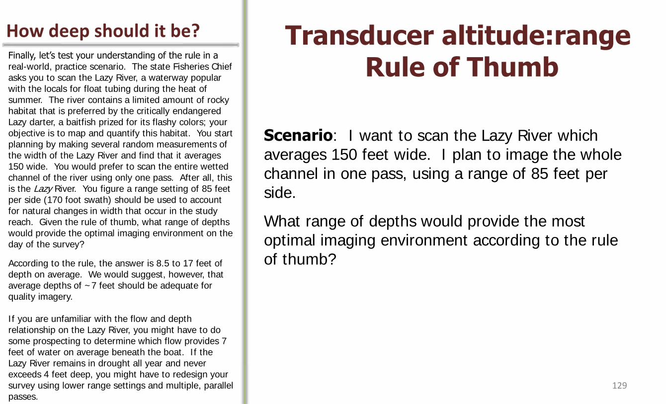
How deep should it be? Transducer altitude:range Rule of Thumb

Finally, let’s test your understanding of the rule in a real-world, practice scenario. The state Fisheries Chief asks you to scan the Lazy River, a waterway popular with the locals for float tubing during the heat of summer. The river contains a limited amount of rocky habitat that is preferred by the critically endangered Lazy darter, a baitfish prized for its flashy colors; your objective is to map and quantify this habitat. You start planning by making several random measurements of the width of the Lazy River and find that it averages 150 wide. You would prefer to scan the entire wetted channel of the river using only one pass. After all, this is the Lazy River. You figure a range setting of 85 feet per side (170 foot swath) should be used to account for natural changes in width that occur in the study reach. Given the rule of thumb, what range of depths would provide the optimal imaging environment on the day of the survey?

According to the rule, the answer is 8.5 to 17 feet of depth on average. We would suggest, however, that average depths of ~7 feet should be adequate for quality imagery. If you are unfamiliar with the flow and depth relationship on the Lazy River, you might have to do some prospecting to determine which flow provides 7 feet of water on average beneath the boat. If the Lazy River remains in drought all year and never exceeds 4 feet deep, you might have to redesign your survey using lower range settings and multiple, parallel passes.

Scenario: I want to scan the Lazy River which averages 150 feet wide. I plan to image the whole channel in one pass, using a range of 85 feet per side.

What range of depths would provide the most optimal imaging environment according to the rule of thumb?

129

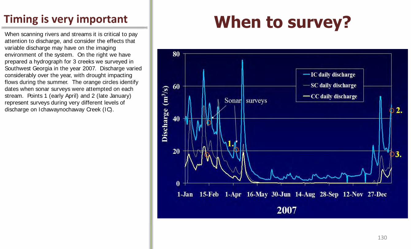
Timing is very important When to survey? When scanning rivers and streams it is critical to pay attention to discharge, and consider the effects that variable discharge may have on the imaging environment of the system. On the right we have prepared a hydrograph for 3 creeks we surveyed in Southwest Georgia in the year 2007. Discharge varied considerably over the year, with drought impacting flows during the summer. The orange circles identify dates when sonar surveys were attempted on each stream. Points 1 (early April) and 2 (late January) represent surveys during very different levels of discharge on Ichawaynochaway Creek (IC).

130

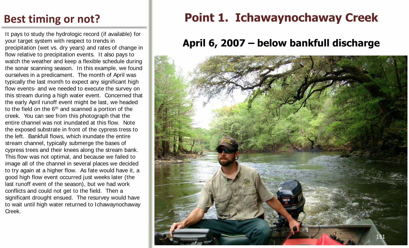
Best timing or not? Point 1. Ichawaynochaway Creek

April 6, 2007 – below bankfull discharge It pays to study the hydrologic record (if available) for your target system with respect to trends in precipitation (wet vs. dry years) and rates of change in flow relative to precipitation events. It also pays to watch the weather and keep a flexible schedule during the sonar scanning season. In this example, we found ourselves in a predicament. The month of April was typically the last month to expect any significant high flow events- and we needed to execute the survey on this stream during a high water event. Concerned that the early April runoff event might be last, we headed to the field on the 6th and scanned a portion of the creek. You can see from this photograph that the entire channel was not inundated at this flow. Note the exposed substrate in front of the cypress tress to the left. Bankfull flows, which inundate the entire stream channel, typically submerge the bases of cypress trees and their knees along the stream bank. This flow was not optimal, and because we failed to image all of the channel in several places we decided to try again at a higher flow. As fate would have it, a good high flow event occurred just weeks later (the last runoff event of the season), but we had work conflicts and could not get to the field. Then a significant drought ensued. The resurvey would have to wait until high water returned to Ichawaynochaway Creek.

131

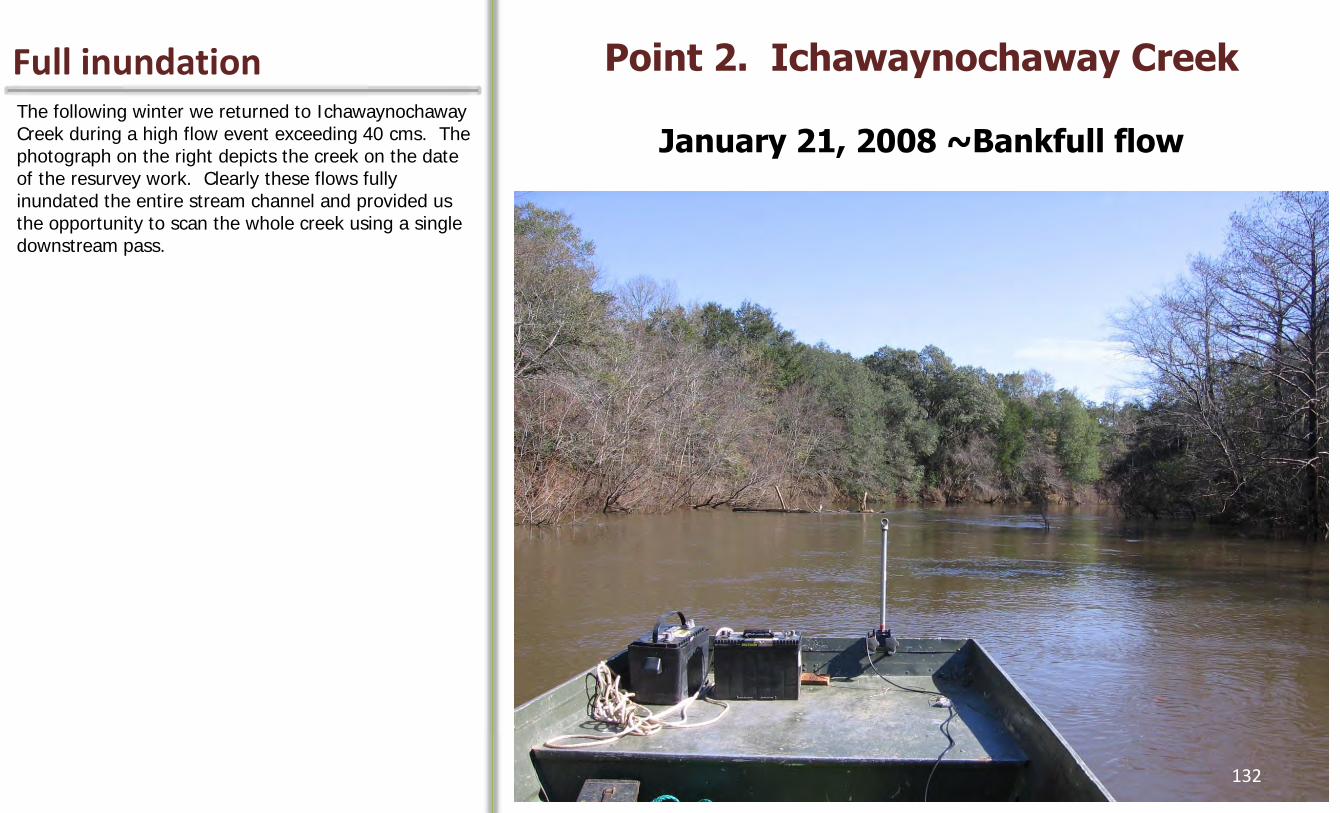
Full inundation Point 2. Ichawaynochaway Creek

January 21, 2008 ~Bankfull flow The following winter we returned to Ichawaynochaway Creek during a high flow event exceeding 40 cms. The photograph on the right depicts the creek on the date of the resurvey work. Clearly these flows fully inundated the entire stream channel and provided us the opportunity to scan the whole creek using a single downstream pass.

132

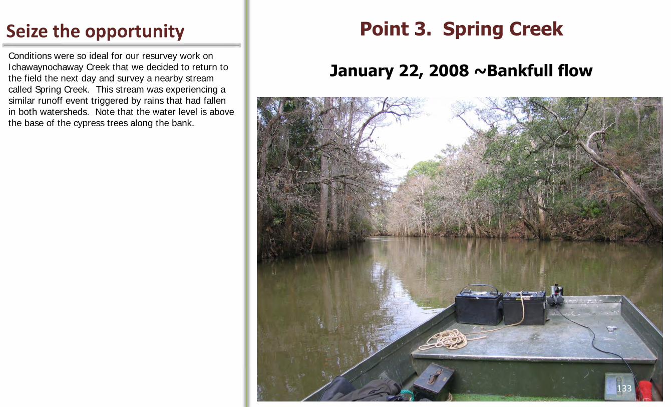
Seize the opportunity Point 3. Spring Creek

January 22, 2008 ~Bankfull flow Conditions were so ideal for our resurvey work on Ichawaynochaway Creek that we decided to return to the field the next day and survey a nearby stream called Spring Creek. This stream was experiencing a similar runoff event triggered by rains that had fallen in both watersheds. Note that the water level is above the base of the cypress trees along the bank.

133

Is width a limiting factor? Maximum System Width We have worked in some small creeks, and in some fairly large Coastal Plain rivers (e.g., Apalachicola River (FL) and Altamaha River (GA)) using multiple parallel passes to maintain high image resolution. In very narrow streams, navigation may be an issue due to shallow water, steep gradient, or high sinuosity. We are curious to see what might result from the use of a kayak with a lightweight marine battery and using sonar recordings rather than snapshots to free up the hands for paddling, but have not been faced with the need to explore this possibility. In a mapping study on the lower Flint River we investigated the effects of increasing ranges on image resolution and map accuracy. Results indicated that ranges of <170 feet per side should be maintained when using 455 kHz to limit the amount of uncertainty in the classified substrate map. This recommendation is consistent with the Humminbird manual statement regarding 150 feet per side as the upper range performance limit at 455 kHz.

• We have mapped rivers 20-350 m wide

• HB 997c SI max width setting is 120 m (360 feet) per side, or 240 m total width

• But remember as range increases, resolution decreases! In wide rivers, an alternative approach would be to make 2 or more passes.

• Our working rule of thumb- for <10% map uncertainty (image distortion) using 455 kHz, use ranges < 170 ft per side (53 m/side). Thus, one-pass approach feasible in rivers up to 300 ft (100 m) wide.

134

Range vs. map uncertainty Range Affects Map Uncertainty It should be very clear at this point that the range setting has global influence on the quality of sonar imagery and products that come from interpretation of the imagery. To further illustrate this point we have included one of the figures from Kaeser et al. (2012) illustrating the relationship between range setting and the areal proportion of the riverbed that was classified as “unsure” due to poor image quality along the river margins. This data set was used to identify the 170 foot threshold discussed in the previous slide.

Range Setting (feet per side)

% U

nsu

re A

rea

in

Ma

p

Lower Flint River Map Project

135

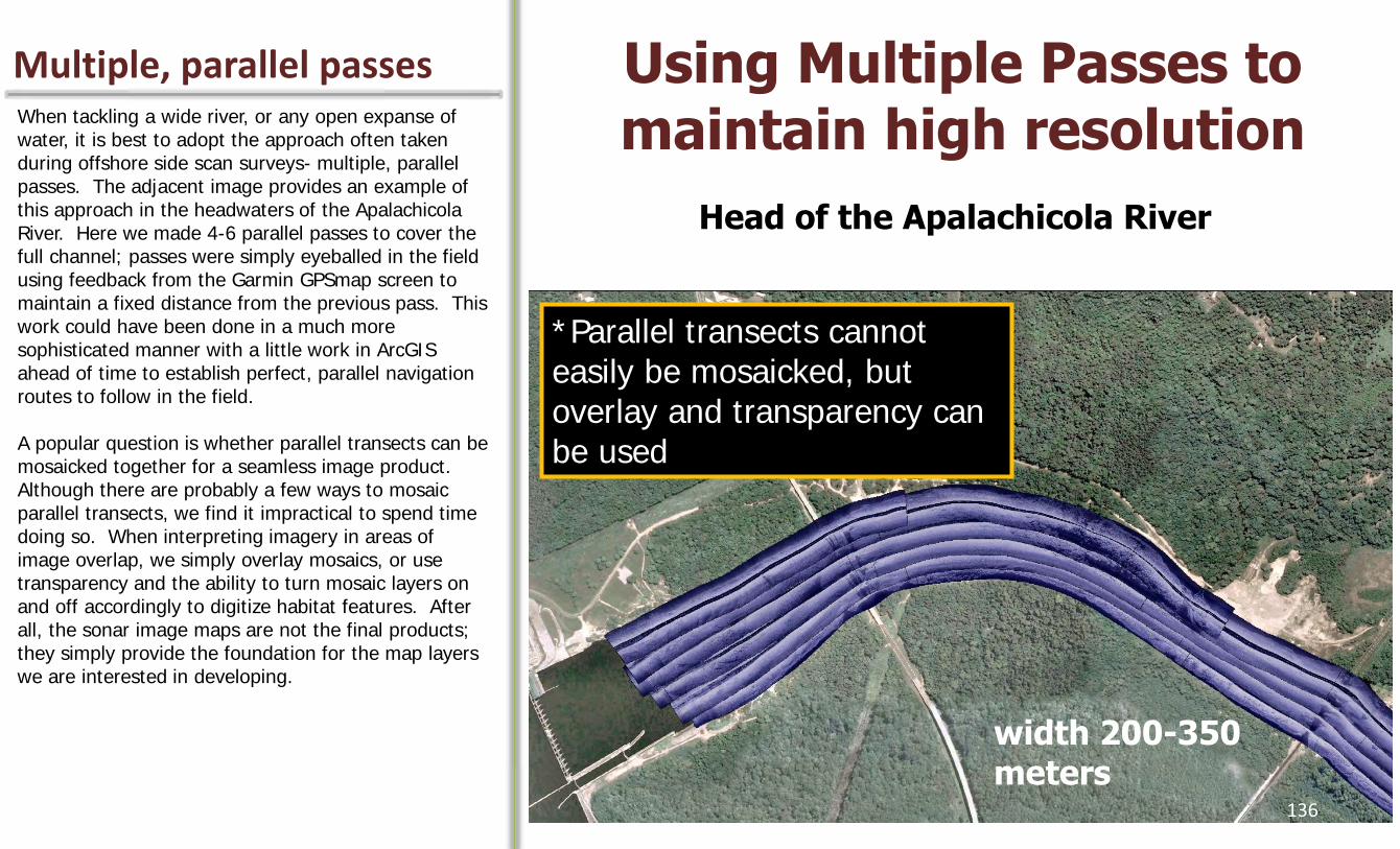
Multiple, parallel passes Using Multiple Passes to maintain high resolution When tackling a wide river, or any open expanse of

water, it is best to adopt the approach often taken during offshore side scan surveys- multiple, parallel passes. The adjacent image provides an example of this approach in the headwaters of the Apalachicola River. Here we made 4-6 parallel passes to cover the full channel; passes were simply eyeballed in the field using feedback from the Garmin GPSmap screen to maintain a fixed distance from the previous pass. This work could have been done in a much more sophisticated manner with a little work in ArcGIS ahead of time to establish perfect, parallel navigation routes to follow in the field. A popular question is whether parallel transects can be mosaicked together for a seamless image product. Although there are probably a few ways to mosaic parallel transects, we find it impractical to spend time doing so. When interpreting imagery in areas of image overlap, we simply overlay mosaics, or use transparency and the ability to turn mosaic layers on and off accordingly to digitize habitat features. After all, the sonar image maps are not the final products; they simply provide the foundation for the map layers we are interested in developing.

Head of the Apalachicola River

*Parallel transects cannot easily be mosaicked, but overlay and transparency can be used

width 200-350 meters

136

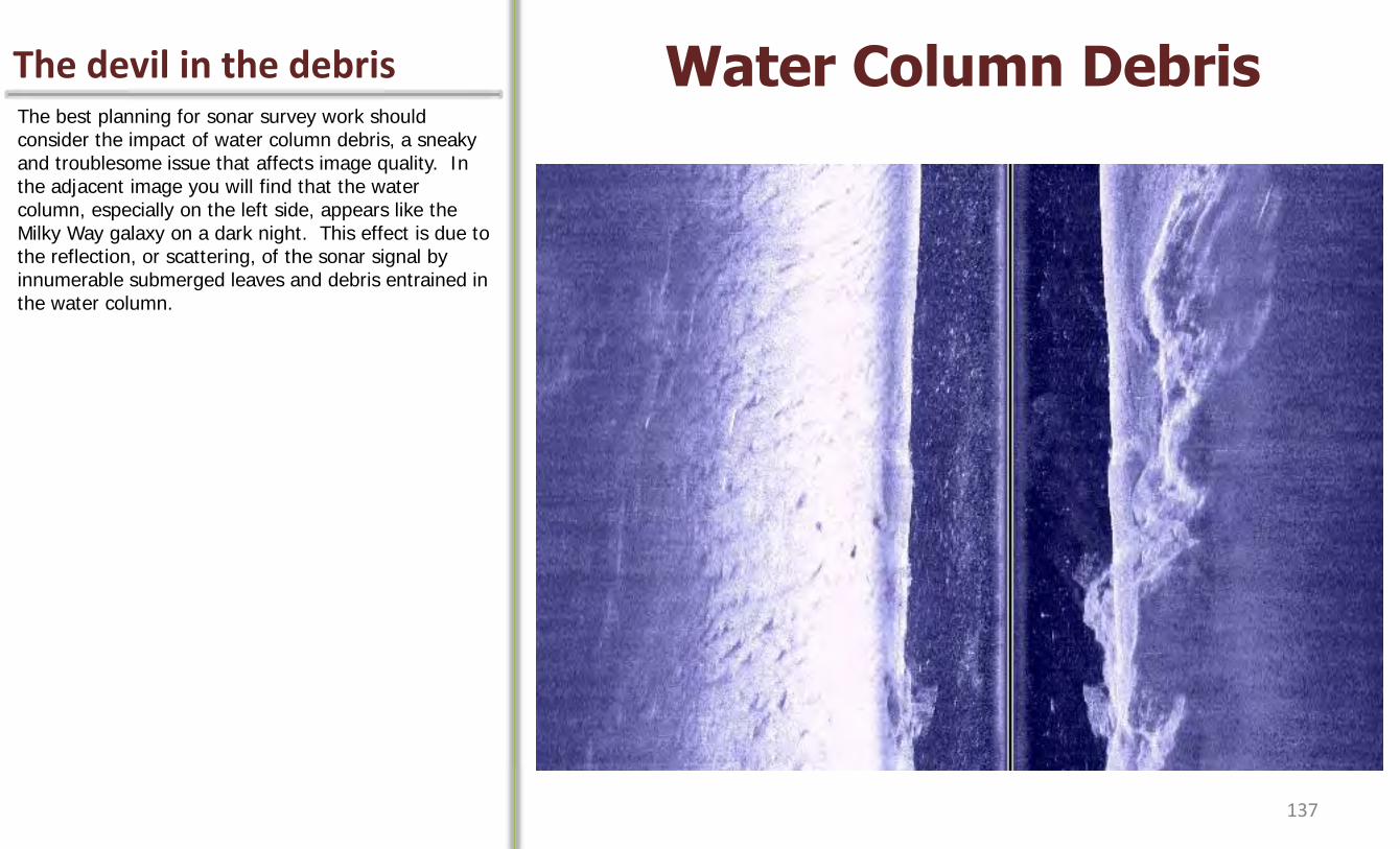
The devil in the debris Water Column Debris The best planning for sonar survey work should consider the impact of water column debris, a sneaky and troublesome issue that affects image quality. In the adjacent image you will find that the water column, especially on the left side, appears like the Milky Way galaxy on a dark night. This effect is due to the reflection, or scattering, of the sonar signal by innumerable submerged leaves and debris entrained in the water column.

137

A look at what’s below Water Column Debris Switching the control head display to the traditional, down-looking sonar view reveals a water column that is full of suspended, sound-scattering debris. This situation is indeed problematic because there isn’t much that can be done operationally to control the impact of debris on image quality. By adjusting the sensitivity setting, some of the noise created by the scattering of signal might be reduced to improve image quality, yet we find it best to try to avoid this situation in the first place, if possible.

138

Ideas for avoiding debris Avoiding Debris When it comes to producing the best possible imagery, there’s no substitute for experience and attention to the dynamic imaging environment of a particular study system. In our experience with scanning creeks and rivers of the Southeast Coastal Plain, we have found that the first high water event of the wet season (which may not occur until January or February in some years) will often be associated with heavy volumes of suspended organic matter, particulary leaves that have been shed during Fall within the riparian zone of the stream and its feeder tributaries. We believe that best practices avoid scanning during the first few high water events that follow leaf drop; we prefer events that occur later in spring (March/April) for water carrying less debris. We also prefer scanning during the falling limb of the hydrograph, rather than during rising water levels. In theory, rising water levels may be working to entrain debris along the banks. Pushing a large wake while running upriver might also have the same effect. It’s difficult to know for sure if these effects are real, nonetheless we try to do everything in our power to scan during the most favorable imaging conditions.

Do not plan sonar survey during first high water event of the wet season

-Rising water levels may entrain debris along bank

-Pushing a wake during an upstream run might also entrain debris

139

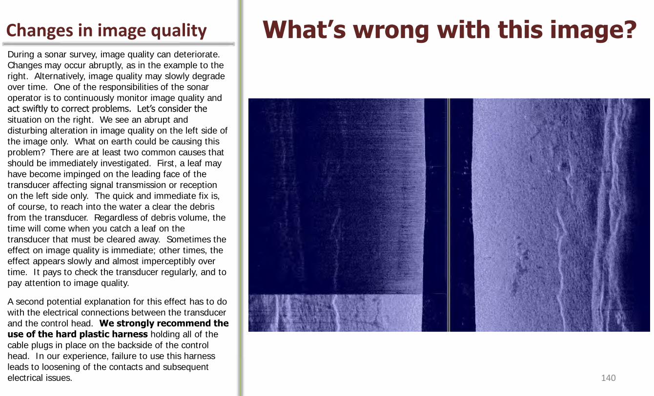
Changes in image quality What’s wrong with this image? During a sonar survey, image quality can deteriorate. Changes may occur abruptly, as in the example to the right. Alternatively, image quality may slowly degrade over time. One of the responsibilities of the sonar operator is to continuously monitor image quality and act swiftly to correct problems. Let’s consider the situation on the right. We see an abrupt and disturbing alteration in image quality on the left side of the image only. What on earth could be causing this problem? There are at least two common causes that should be immediately investigated. First, a leaf may have become impinged on the leading face of the transducer affecting signal transmission or reception on the left side only. The quick and immediate fix is, of course, to reach into the water a clear the debris from the transducer. Regardless of debris volume, the time will come when you catch a leaf on the transducer that must be cleared away. Sometimes the effect on image quality is immediate; other times, the effect appears slowly and almost imperceptibly over time. It pays to check the transducer regularly, and to pay attention to image quality.

A second potential explanation for this effect has to do with the electrical connections between the transducer and the control head. We strongly recommend the use of the hard plastic harness holding all of the cable plugs in place on the backside of the control head. In our experience, failure to use this harness leads to loosening of the contacts and subsequent electrical issues. 140

Turbulence affects quality Water Column Turbulence Turbulent flow can also have a negative effect on image quality. In the example on the right we see what appears to be plume of milky water within the left side of the water column. This effect is reminiscent of a plume of suspended sediment, however, the entire creek was incredibly muddy on the day this image was captured. This effect is actually a visualization of turbulent water column flow, rather than a sediment plume. The scattering of sound that occurs in a turbulent environment tends to degrade image quality to an extent. In this example, turbulent flow is being created where high water velocity intercepts deflecting structure.

141

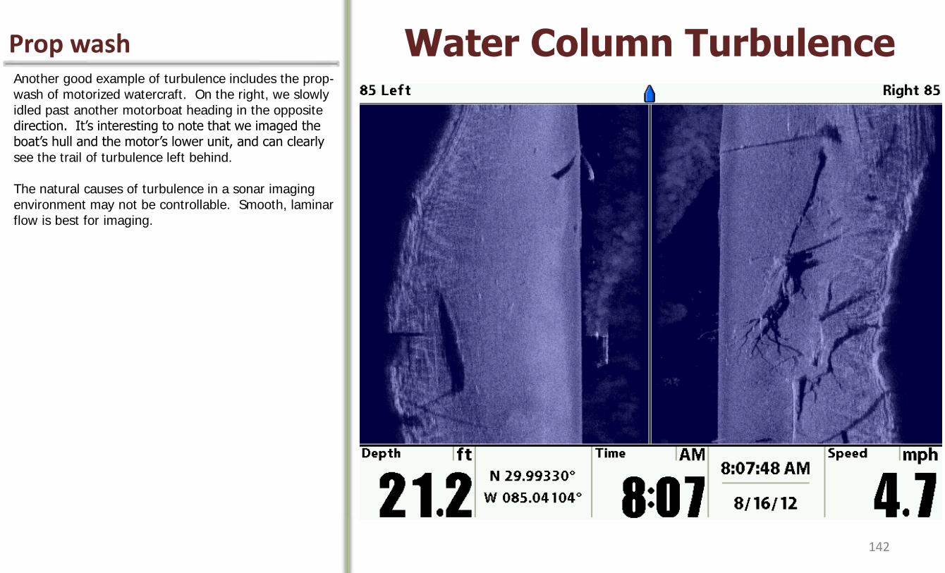
Prop wash Water Column Turbulence Another good example of turbulence includes the prop-wash of motorized watercraft. On the right, we slowly idled past another motorboat heading in the opposite direction. It’s interesting to note that we imaged the boat’s hull and the motor’s lower unit, and can clearly see the trail of turbulence left behind. The natural causes of turbulence in a sonar imaging environment may not be controllable. Smooth, laminar flow is best for imaging.

142

Imaging rough reaches Navigating Heavy Shoals

Missing data

Here is a mosaic of raw sonar images captured during navigation through a set of treacherous shoals and rough water. The shallow rocks cast a lot of sonar shadow; between the outcrops turbulence has created some image wash-out. Despite these effects, there is still a lot of useful information contained in this mosaic. The shadowed areas can either be classified as missing data, or assigned a substrate classification with the aid of an air photo or field notes. Note just how close the transducer came to striking the boulders in this reach! In 6 years we have never lost a transducer to a rock. Would you be willing to take these kind of calculated risks with a towfish and a $30,000+ sonar system? Confidence in the ability to scan a variety of systems and situations is a direct benefit of low-cost equipment.

143

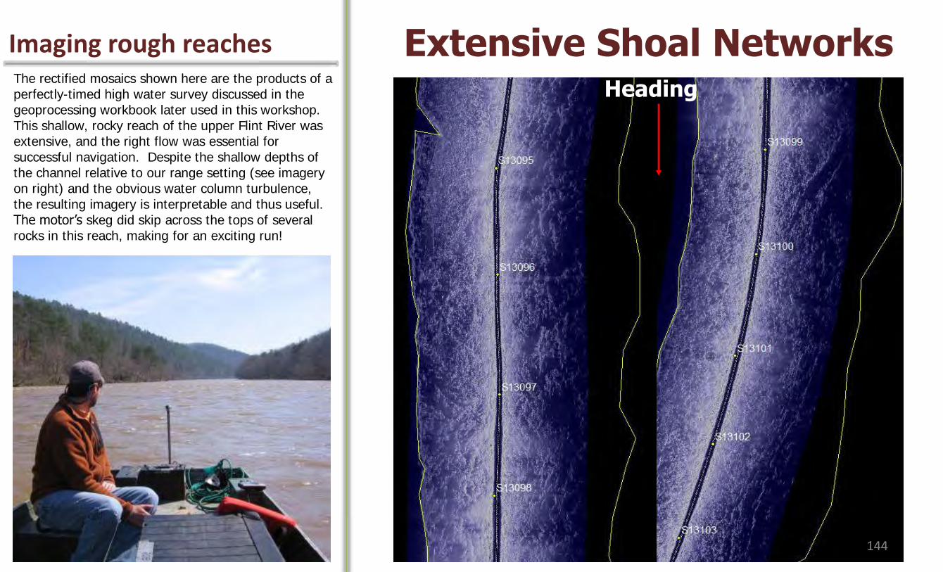
Imaging rough reaches Extensive Shoal Networks The rectified mosaics shown here are the products of a perfectly-timed high water survey discussed in the geoprocessing workbook later used in this workshop. This shallow, rocky reach of the upper Flint River was extensive, and the right flow was essential for successful navigation. Despite the shallow depths of the channel relative to our range setting (see imagery on right) and the obvious water column turbulence, the resulting imagery is interpretable and thus useful. The motor’s skeg did skip across the tops of several rocks in this reach, making for an exciting run!

Heading

144

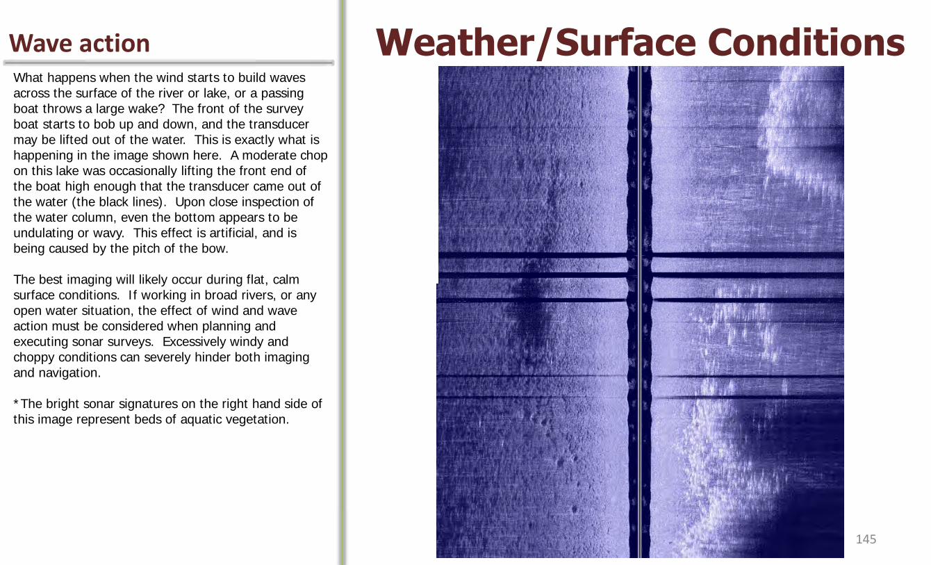
Wave action Weather/Surface Conditions What happens when the wind starts to build waves across the surface of the river or lake, or a passing boat throws a large wake? The front of the survey boat starts to bob up and down, and the transducer may be lifted out of the water. This is exactly what is happening in the image shown here. A moderate chop on this lake was occasionally lifting the front end of the boat high enough that the transducer came out of the water (the black lines). Upon close inspection of the water column, even the bottom appears to be undulating or wavy. This effect is artificial, and is being caused by the pitch of the bow. The best imaging will likely occur during flat, calm surface conditions. If working in broad rivers, or any open water situation, the effect of wind and wave action must be considered when planning and executing sonar surveys. Excessively windy and choppy conditions can severely hinder both imaging and navigation. *The bright sonar signatures on the right hand side of this image represent beds of aquatic vegetation.

145

Best to avoid Traffic Traffic on the water can come in many forms: anchored boats, jet skiers, kayakers, bass fisherman, swimmers, sunbathers, deadhead loggers, you name it! When you are in the middle of a long, uninterrupted survey transect, the last thing you want to do is detour around traffic or have to stop altogether. Let’s discuss the example shown here. Our objective was to conduct a shoreline habitat survey in a reservoir cove. We determined that 85 feet per side range would allow us to generate high resolution data while passing directly in front of dozens of docks and piers (actual boat path in blue). When do you think we conducted this survey? February- when noone was out on the docks fishing or enjoying a brew.

This concludes Session II- Part A on Mission Planning. Next we will discuss the field execution of the sonar mission.

146

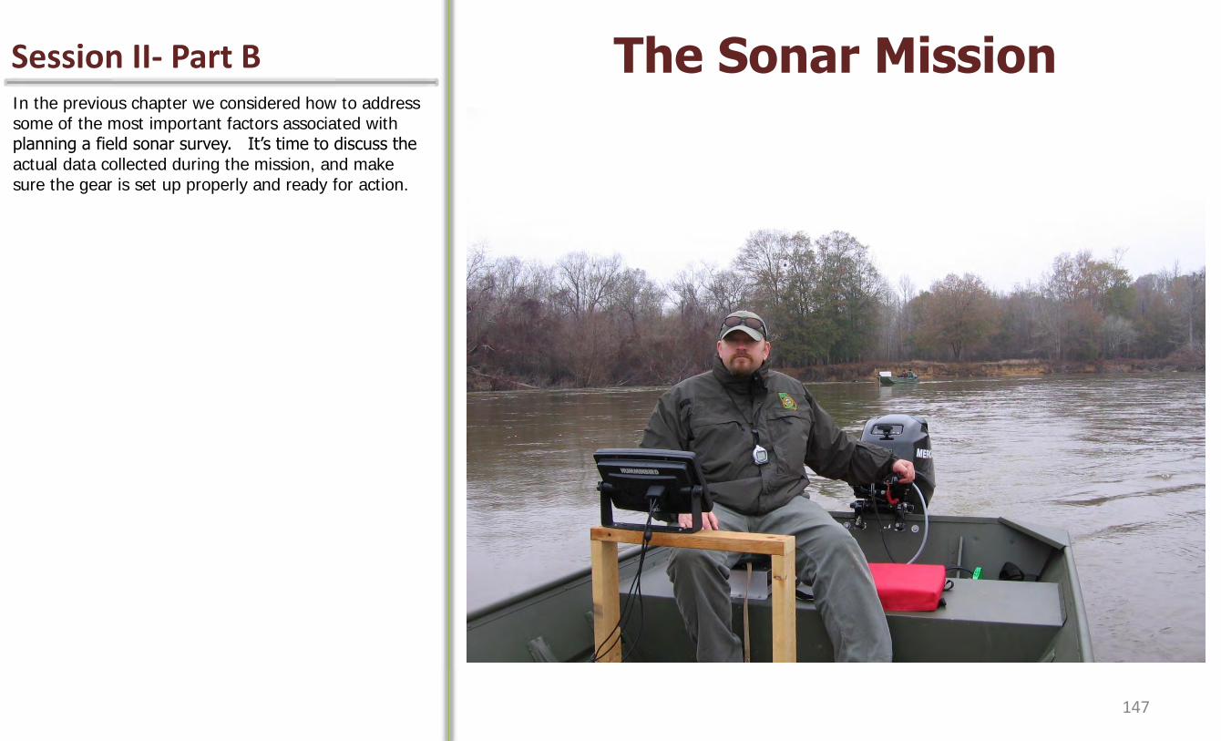
Session II- Part B The Sonar Mission In the previous chapter we considered how to address some of the most important factors associated with planning a field sonar survey. It’s time to discuss the actual data collected during the mission, and make sure the gear is set up properly and ready for action.

147

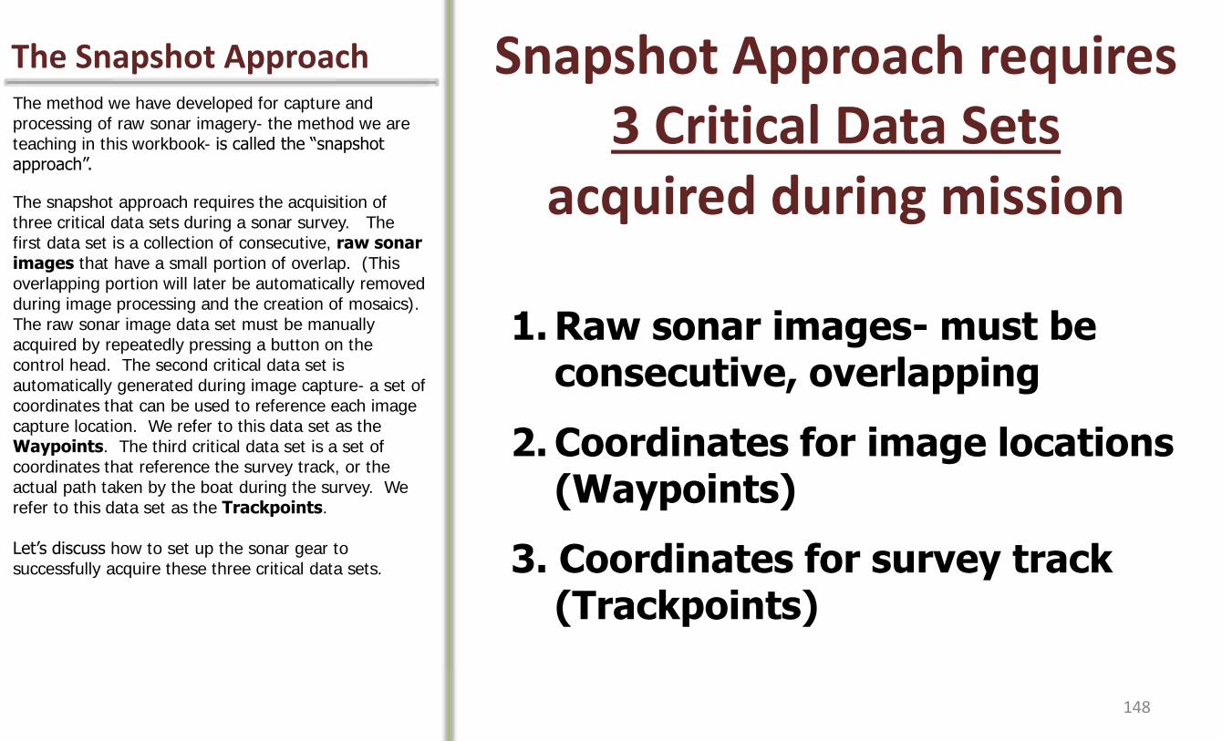
The Snapshot Approach Snapshot Approach requires 3 Critical Data Sets

acquired during mission

The method we have developed for capture and processing of raw sonar imagery- the method we are teaching in this workbook- is called the “snapshot approach”.

The snapshot approach requires the acquisition of three critical data sets during a sonar survey. The first data set is a collection of consecutive, raw sonar images that have a small portion of overlap. (This overlapping portion will later be automatically removed during image processing and the creation of mosaics). The raw sonar image data set must be manually acquired by repeatedly pressing a button on the control head. The second critical data set is automatically generated during image capture- a set of coordinates that can be used to reference each image capture location. We refer to this data set as the Waypoints. The third critical data set is a set of coordinates that reference the survey track, or the actual path taken by the boat during the survey. We refer to this data set as the Trackpoints. Let’s discuss how to set up the sonar gear to successfully acquire these three critical data sets.

1. Raw sonar images- must be consecutive, overlapping

2. Coordinates for image locations (Waypoints)

3. Coordinates for survey track (Trackpoints)

148

The Control Head Boat Configuration Control Head Placement

The sonar control head should be placed near to, or directly in front of the boat operator as shown in this photo. Sonar surveys can easily be conducted by a one person. This one person will simultaneously drive the boat and manipulate the sonar gear. Hundreds of miles of streams have been surveyed in this manner. While a survey is underway, the boat operator will typically need the feedback provided by the on-screen imagery to maintain proper boat position. For example, the apparent position of the stream banks in the imagery helps the boat operator maintain position in the middle of the river channel, or maintain a fixed distance from the lakeshore. The control head should, thus, be close enough and at the proper level for the boat operator to see the screen and reach the buttons. With a little creativity just about any boat can be properly outfitted with the control head. In this example, we built a platform out of scrap wood in the garage that we bolted to the side and floor of the boat. This frame carried our original 981c SI control head for surveys over a 5-year period. Not fancy but functional. *Although a holster for the GPS was attached to this platform, the GPS was actually placed adjacent to the transducer during surveys- not on this console.

149

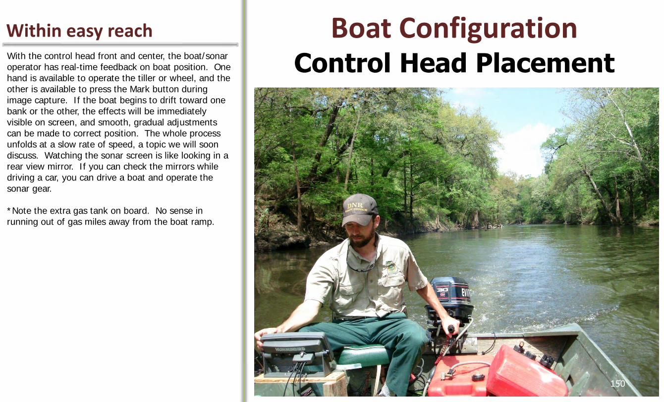
Within easy reach Boat Configuration Control Head Placement

With the control head front and center, the boat/sonar operator has real-time feedback on boat position. One hand is available to operate the tiller or wheel, and the other is available to press the Mark button during image capture. If the boat begins to drift toward one bank or the other, the effects will be immediately visible on screen, and smooth, gradual adjustments can be made to correct position. The whole process unfolds at a slow rate of speed, a topic we will soon discuss. Watching the sonar screen is like looking in a rear view mirror. If you can check the mirrors while driving a car, you can drive a boat and operate the sonar gear. *Note the extra gas tank on board. No sense in running out of gas miles away from the boat ramp.

150

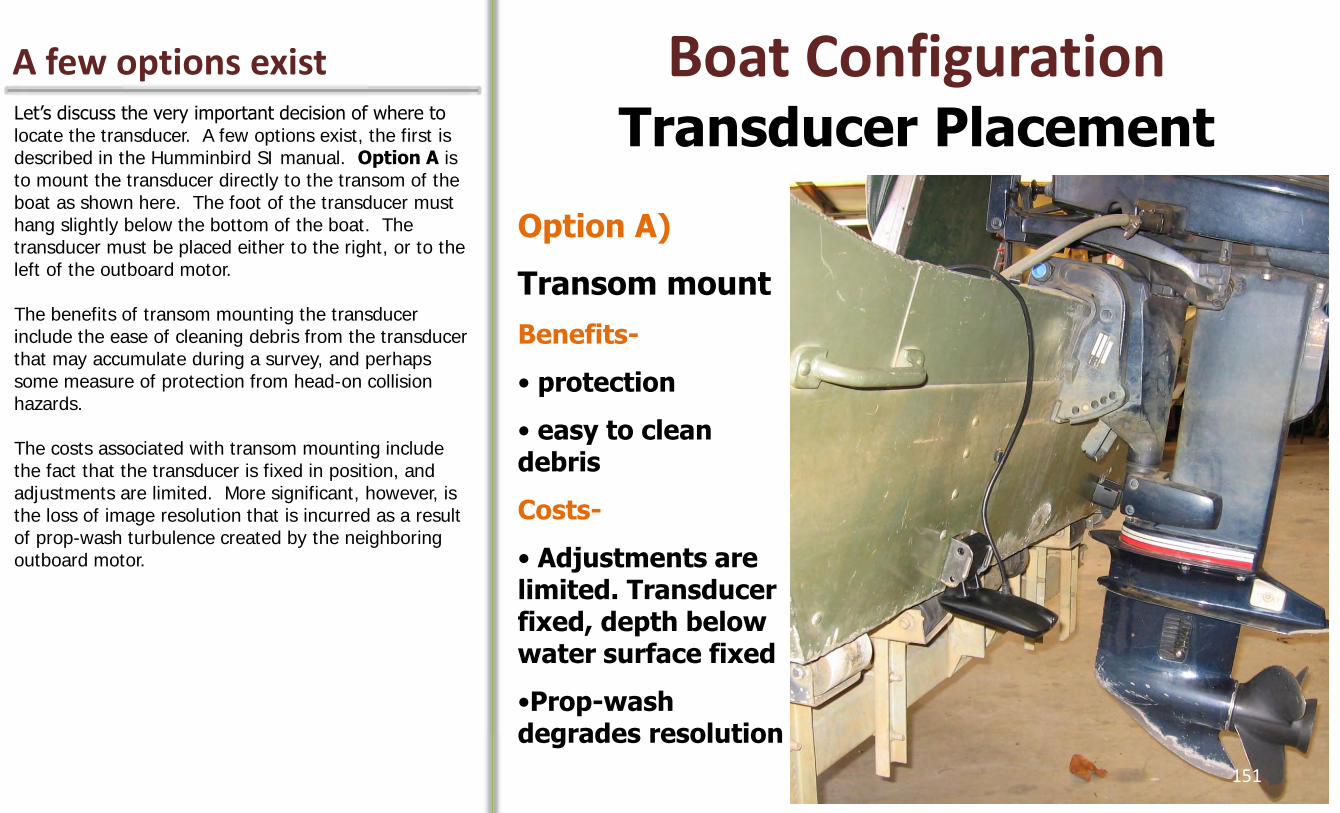
A few options exist Boat Configuration Transducer Placement

Let’s discuss the very important decision of where to locate the transducer. A few options exist, the first is described in the Humminbird SI manual. Option A is to mount the transducer directly to the transom of the boat as shown here. The foot of the transducer must hang slightly below the bottom of the boat. The transducer must be placed either to the right, or to the left of the outboard motor. The benefits of transom mounting the transducer include the ease of cleaning debris from the transducer that may accumulate during a survey, and perhaps some measure of protection from head-on collision hazards. The costs associated with transom mounting include the fact that the transducer is fixed in position, and adjustments are limited. More significant, however, is the loss of image resolution that is incurred as a result of prop-wash turbulence created by the neighboring outboard motor.

Option A)

Transom mount

Benefits-

• protection

• easy to clean debris

Costs-

• Adjustments are limited. Transducer fixed, depth below water surface fixed

•Prop-wash degrades resolution

151

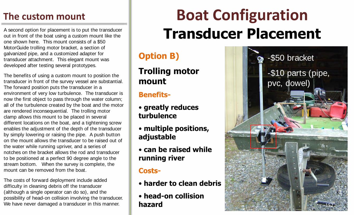
The custom mount Boat Configuration Transducer Placement

A second option for placement is to put the transducer out in front of the boat using a custom mount like the one shown here. This mount consists of a $50 MotorGuide trolling motor bracket, a section of galvanized pipe, and a customized adapter for transducer attachment. This elegant mount was developed after testing several prototypes.

The benefits of using a custom mount to position the transducer in front of the survey vessel are substantial. The forward position puts the transducer in a environment of very low turbulence. The transducer is now the first object to pass through the water column; all of the turbulence created by the boat and the motor are rendered inconsequential. The trolling motor clamp allows this mount to be placed in several different locations on the boat, and a tightening screw enables the adjustment of the depth of the transducer by simply lowering or raising the pipe. A push button on the mount allows the transducer to be raised out of the water while running upriver, and a series of notches on the bracket allows the rod and transducer to be positioned at a perfect 90 degree angle to the stream bottom. When the survey is complete, the mount can be removed from the boat.

The costs of forward deployment include added difficulty in cleaning debris off the transducer (although a single operator can do so), and the possibility of head-on collision involving the transducer. We have never damaged a transducer in this manner.

Option B)

Trolling motor mount

Benefits-

• greatly reduces turbulence

• multiple positions, adjustable

• can be raised while running river

Costs-

• harder to clean debris

• head-on collision hazard

-$50 bracket

-$10 parts (pipe, pvc, dowel)

152

Attaching the transducer Boat Configuration Transducer Adapter

To attach the transducer to the end of the pipe, we took an appropriately sized PVC T-connector, cut the wing ends off with a hack saw, and used a rubber mallet to pound a small section of wooden dowel, that had been sanded to size, into the connector. We then used a drill press to drill a perfect hole through the dowel to accommodate the hardware used to attach the transducer. This small adapter (shown right) works superbly, except that between surveys the wooden dowel may dry out and shrink within the PVC piece, causing the transducer to pivot freely. To circumvent this problem, we remove the transducer and the PVC adapter after each survey, and place the adapter in a small, sealed jar of water. This little jar is stored in our equipment kit. The dowel never dries out, and remains fixed inside the PVC piece ready for the next survey. Another option that works perfectly is to use a galvanized fitting like the one shown below, drilled out to accommodate the attachment hardware.

•3/4” outside diameter, (sold as 1/2” inside diameter) pipe

•T-bar pvc joint

•Wooden dowel insert

153

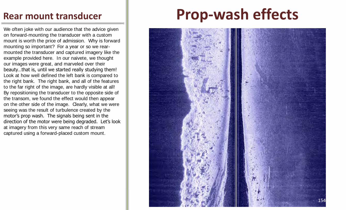
Rear mount transducer Prop-wash effects We often joke with our audience that the advice given on forward-mounting the transducer with a custom mount is worth the price of admission. Why is forward mounting so important? For a year or so we rear-mounted the transducer and captured imagery like the example provided here. In our naivete, we thought our images were great, and marveled over their beauty…that is, until we started really studying them! Look at how well defined the left bank is compared to the right bank. The right bank, and all of the features to the far right of the image, are hardly visible at all! By repositioning the transducer to the opposite side of the transom, we found the effect would then appear on the other side of the image. Clearly, what we were seeing was the result of turbulence created by the motor’s prop wash. The signals being sent in the direction of the motor were being degraded. Let’s look at imagery from this very same reach of stream captured using a forward-placed custom mount.

154

Forward mount transducer No Prop-wash effects The differences are striking to say the least! Using a forward mounted transducer the right hand side of the image is now perfectly clear, and similar in quality to the left side. Low and behold, a nice cache of deadhead logs and other woody debris is now visible in the upper right corner of the image. This cache was invisible to us when using the rear mounted transducer.

155

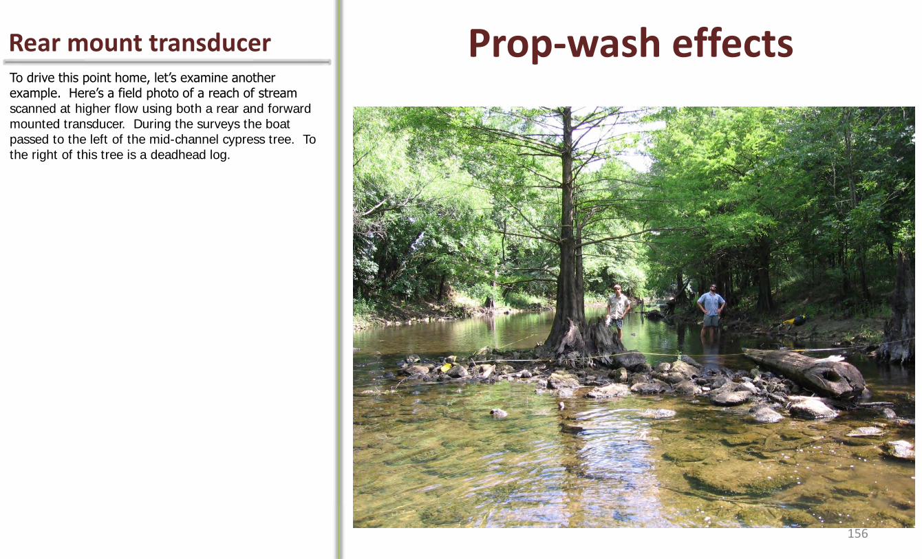
Rear mount transducer Prop-wash effects To drive this point home, let’s examine another example. Here’s a field photo of a reach of stream scanned at higher flow using both a rear and forward mounted transducer. During the surveys the boat passed to the left of the mid-channel cypress tree. To the right of this tree is a deadhead log.

156

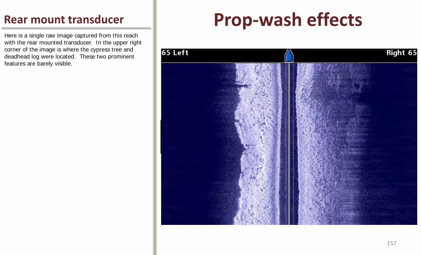
Rear mount transducer Prop-wash effects Here is a single raw image captured from this reach with the rear mounted transducer. In the upper right corner of the image is where the cypress tree and deadhead log were located. These two prominent features are barely visible.

157

Forward mount transducer No Prop-wash Here is the imagery produced using a forward-mounted transducer. The improvement in image quality is extraordinary. The cypress tree and its sonar shadow are clearly visible, and so is the large deadhead log that was resting between the tree and the right bank. The right bank is now clearly discernible. We strongly recommend to all sonar operators to consider building a custom mount that enables the forward placement of the transducer. We simply would not consider capturing sonar imagery for mapping purposes any other way.

158

Go with the flow Heading Upstream or Down? Since we are on the topic of minimizing turbulence for the sake of producing the highest quality imagery, let’s discuss a few more best practices. A very relevant question having to do with survey execution is whether to head upstream or down. We have found that heading downstream produces higher quality imagery, and believe this result is attributable to less turbulence around the transducer when going with the flow of the river rather than pushing upstream against it.

There are a couple of negatives associated with going downstream, although they do not outweigh the benefits. One downside is that you don’t get to see what is around the next corner. In a swift, confined stream, this might be a hazardous situation. We recommend launching the boat at a downstream ramp and heading upstream to your survey starting point. Along the way you can take mental notes on the condition of the stream and any navigational hazards. Swift decisions must be made when such hazards are encountered, and when the survey is underway it’s best to have these things figured out. Heading upriver to start the day is always a good idea. If your motor dies you can float back to the ramp. If you encounter shallow, treacherous areas, your ability to power upstream and beyond such hazards will almost always be rewarded with successful downstream passage. The opposite case is NOT always true!

In a bend, the river will try to sweep your boat toward the outside bank. Offset this force with gradual thrust away from the bank.

Downstream (usually) is best, but Why?

Less turbulence around transducer, smoother ride= higher quality images

Go with the flow!

Caution- Navigation can be treacherous

159

It’s the little things Ballast to stabilize bow Another practice we highly recommend is the use of ballast to stabilize the front of the boat. By loading the front end, the effect of minor wave action on the pitch and roll of the boat is minimized. This added stability pays dividends in enhanced image quality. Lots of things that are hanging around in your garage can be used as ballast. We have used cinder blocks and old marine batteries as shown here. The downside is lugging around all this extra weight. One day it dawned on us that we could take an old, oversized cooler, put it on the front end of the boat, and fill it with a pail or a bilge pump before initiating the survey. When finished, the water weight can simply be dumped overboard. Let’s face it, we’re trying our best to produce high quality imagery with a $3000 piece of equipment. Every little thing, however insignificant, might contribute to the production of high quality imagery throughout a survey. If you have a crew member on board, you might also want to avoid having this person up and moving around the boat during the survey. Boat stability is a virtue worth pursuing.

Ballast

160

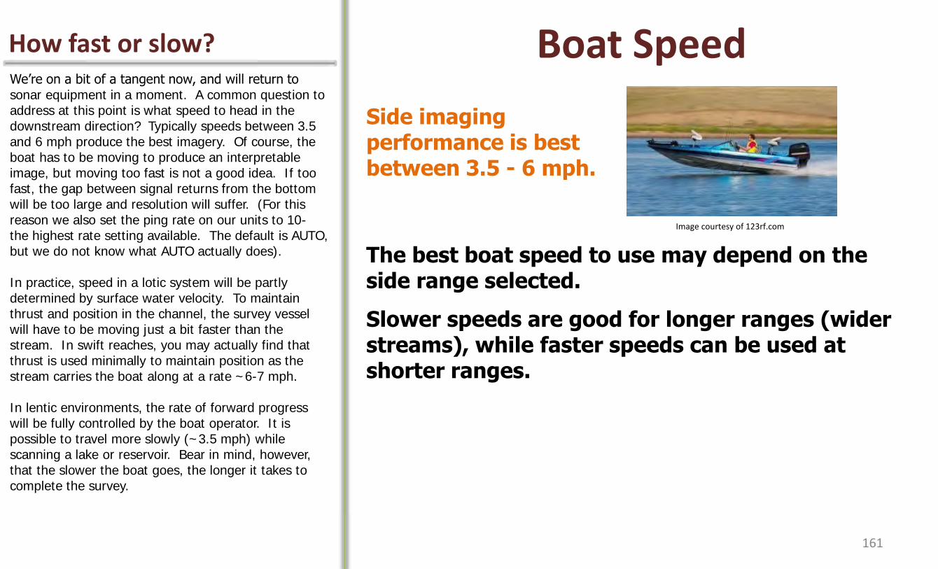
How fast or slow? Boat Speed We’re on a bit of a tangent now, and will return to sonar equipment in a moment. A common question to address at this point is what speed to head in the downstream direction? Typically speeds between 3.5 and 6 mph produce the best imagery. Of course, the boat has to be moving to produce an interpretable image, but moving too fast is not a good idea. If too fast, the gap between signal returns from the bottom will be too large and resolution will suffer. (For this reason we also set the ping rate on our units to 10- the highest rate setting available. The default is AUTO, but we do not know what AUTO actually does). In practice, speed in a lotic system will be partly determined by surface water velocity. To maintain thrust and position in the channel, the survey vessel will have to be moving just a bit faster than the stream. In swift reaches, you may actually find that thrust is used minimally to maintain position as the stream carries the boat along at a rate ~6-7 mph. In lentic environments, the rate of forward progress will be fully controlled by the boat operator. It is possible to travel more slowly (~3.5 mph) while scanning a lake or reservoir. Bear in mind, however, that the slower the boat goes, the longer it takes to complete the survey.

The best boat speed to use may depend on the side range selected.

Slower speeds are good for longer ranges (wider streams), while faster speeds can be used at shorter ranges.

Side imaging performance is best between 3.5 - 6 mph.

Image courtesy of 123rf.com

161

Depends on fortitude How far can we go in 1 day? The maximum range, or distance that can be surveyed in one day is around 50 km. After 6 or so hours on the water, driving the boat and pressing buttons, mental fatigue may set in. The pace of 5 mph is quite leisurely, and staying focused on the survey demands mental fortitude. *This range (50 km) can and has been exceeded by our crew of two sonar techs aboard one boat (Reuben Smit and Tanner Williamson). Each would drive and operate the survey boat for a few hours then trade off with the other. Biological necessities were taken care of while the survey was underway. This committed approach yielded continuous, unbroken survey transects that extended for many, many miles. As you will learn later, there are significant benefits to capturing long continuous segments when it comes to image processing.

At 5 mph (8 kmh), it is possible to survey approximately 30 miles (50 km) in a typical day.

162

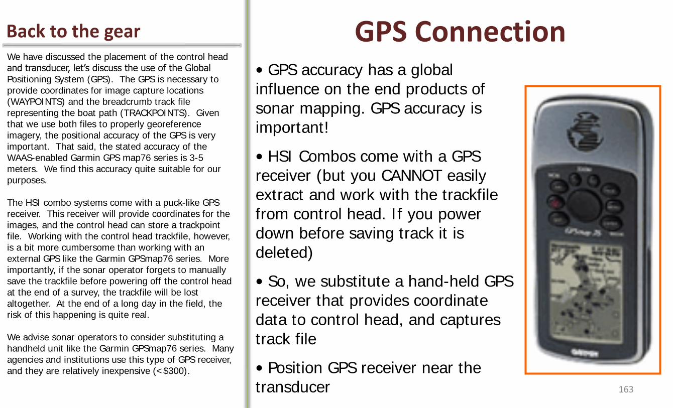
Back to the gear GPS Connection We have discussed the placement of the control head and transducer, let’s discuss the use of the Global Positioning System (GPS). The GPS is necessary to provide coordinates for image capture locations (WAYPOINTS) and the breadcrumb track file representing the boat path (TRACKPOINTS). Given that we use both files to properly georeference imagery, the positional accuracy of the GPS is very important. That said, the stated accuracy of the WAAS-enabled Garmin GPS map76 series is 3-5 meters. We find this accuracy quite suitable for our purposes. The HSI combo systems come with a puck-like GPS receiver. This receiver will provide coordinates for the images, and the control head can store a trackpoint file. Working with the control head trackfile, however, is a bit more cumbersome than working with an external GPS like the Garmin GPSmap76 series. More importantly, if the sonar operator forgets to manually save the trackfile before powering off the control head at the end of a survey, the trackfile will be lost altogether. At the end of a long day in the field, the risk of this happening is quite real. We advise sonar operators to consider substituting a handheld unit like the Garmin GPSmap76 series. Many agencies and institutions use this type of GPS receiver, and they are relatively inexpensive (<$300).

• GPS accuracy has a global influence on the end products of sonar mapping. GPS accuracy is important!

• HSI Combos come with a GPS receiver (but you CANNOT easily extract and work with the trackfile from control head. If you power down before saving track it is deleted)

• So, we substitute a hand-held GPS receiver that provides coordinate data to control head, and captures track file

• Position GPS receiver near the transducer

163

2 Cables are needed How to swap GPS receivers To substitute a Garmin or other handheld GPS unit for the out-of-box receiver you will need to purchase two accessory cables. The first cable is sold only by the Humminbird company through their website. It is called the AS HHGPS cable- Handheld GPS Connection Kit ($24). The cable has the plug that inserts into the back of the control head on one end, and 4 bare wires on the other. The other cable will depend on the type of GPS receiver you are integrating. Our Garmin GPSmap76CSx units require a power/data cable such as shown on the lower right. The connecting plug that inserts into the back of the Garmin is a round, 4-pin plug. The harness includes 4 bare wires, two of which are power wires and the other two are data wires. The only trick is matching the proper wires up. Once wired properly, the Garmin GPS will be able to draw its power from the same power source as the control head, and the control head and GPS will be able to communicate (send data back and forth) with each other. During the wiring process we splice a long (~14 foot) section of 4-strand trailer harness wire between the control head GPS accessory cable and the Garmin power/data cable that lengthens the line and enables us to put the GPS in the front of the boat, next to the transducer mount.

164

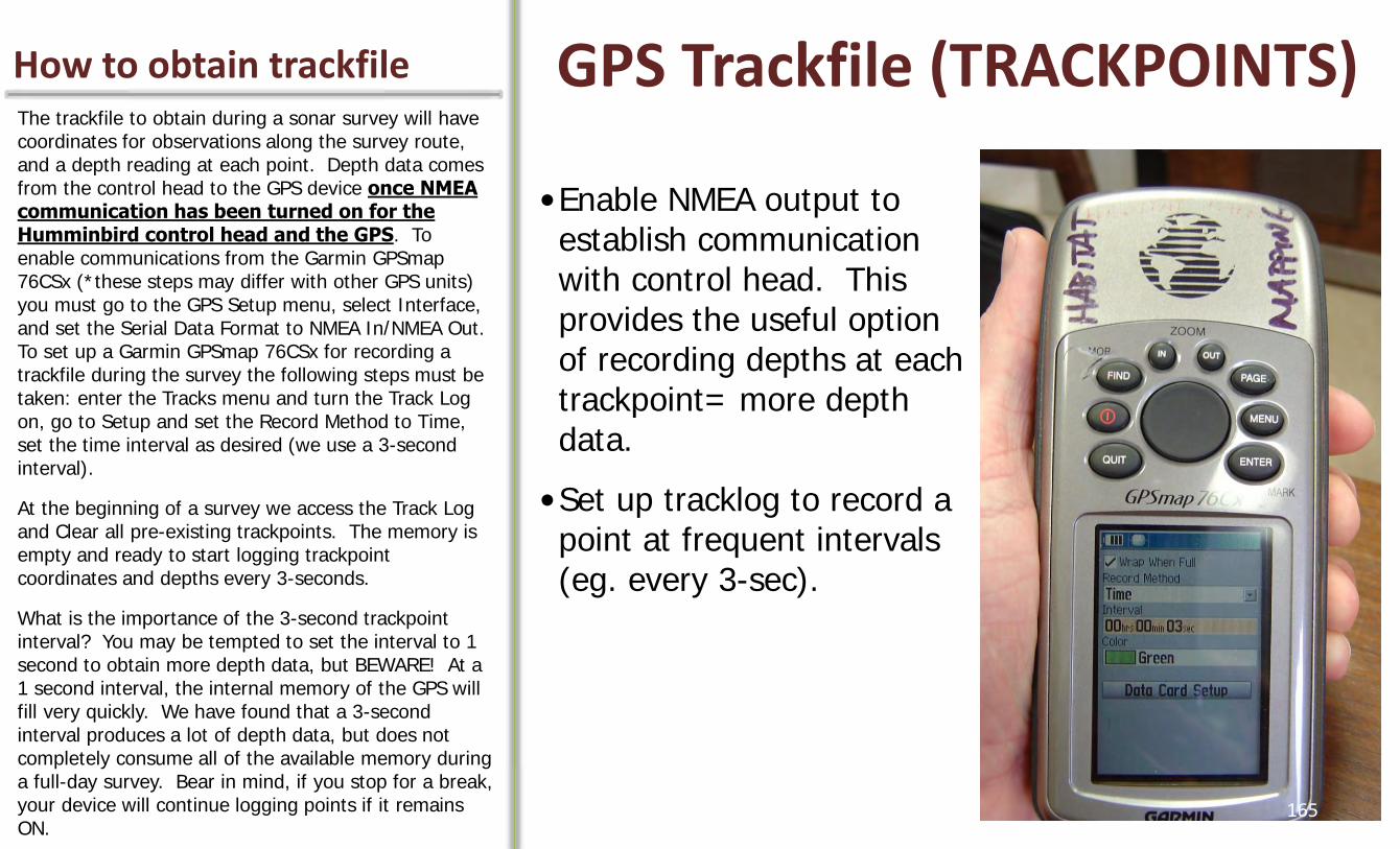
How to obtain trackfile GPS Trackfile (TRACKPOINTS) The trackfile to obtain during a sonar survey will have coordinates for observations along the survey route, and a depth reading at each point. Depth data comes from the control head to the GPS device once NMEA communication has been turned on for the Humminbird control head and the GPS. To enable communications from the Garmin GPSmap 76CSx (*these steps may differ with other GPS units) you must go to the GPS Setup menu, select Interface, and set the Serial Data Format to NMEA In/NMEA Out. To set up a Garmin GPSmap 76CSx for recording a trackfile during the survey the following steps must be taken: enter the Tracks menu and turn the Track Log on, go to Setup and set the Record Method to Time, set the time interval as desired (we use a 3-second interval).

At the beginning of a survey we access the Track Log and Clear all pre-existing trackpoints. The memory is empty and ready to start logging trackpoint coordinates and depths every 3-seconds.

What is the importance of the 3-second trackpoint interval? You may be tempted to set the interval to 1 second to obtain more depth data, but BEWARE! At a 1 second interval, the internal memory of the GPS will fill very quickly. We have found that a 3-second interval produces a lot of depth data, but does not completely consume all of the available memory during a full-day survey. Bear in mind, if you stop for a break, your device will continue logging points if it remains ON.

•Enable NMEA output to establish communication with control head. This provides the useful option of recording depths at each trackpoint= more depth data.

•Set up tracklog to record a point at frequent intervals (eg. every 3-sec).

165

How to set range Although there are many settings that can be manipulated via the control head, the range setting is one that has global influence over image quality as discussed at length in previous chapters. The range setting is accessed via the 1st menu from the side imaging view. The range used during imaging will depend on system size and a variety of survey objectives. To determine the range(s) for a project, we typically first examine streams in Google Earth and make measurements with the ruler tool to assess typical channel variability. If making a single pass to cover the entire wetted channel of a stream, we will select a range setting that is slightly larger than mean stream width to accommodate for natural channel variability. On the water you may find it useful to spend some time practicing with different range settings in a reach with the goal of identifying the ideal setting for your study reach. If surveying a long reach of stream, expect that changes in width will occur as you progress downstream that will necessitate an on-the-fly range change. A good practice is to record the 1st image waypoint number following a change in range setting. Each time the range is changed, one geoprocessing segment ends and a new segment begins (this concept will make sense when we get to geoprocessing). For now, suffice it to say that we want to be conservative with the number of range changes undertaken during a survey. That is why we opt for a setting that will encompass typical channel width variability.

Critical Setting - Range

Range

• Set to encompass typical channel width variability

• Assessment Tools-

1) Examine Google Earth maps

2) Carry rangefinder in field

3) Trial and Error

166

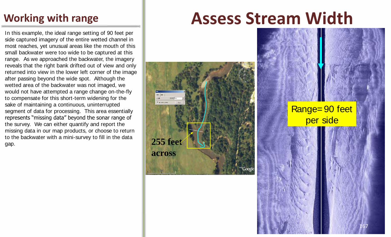
Working with range In this example, the ideal range setting of 90 feet per side captured imagery of the entire wetted channel in most reaches, yet unusual areas like the mouth of this small backwater were too wide to be captured at this range. As we approached the backwater, the imagery reveals that the right bank drifted out of view and only returned into view in the lower left corner of the image after passing beyond the wide spot. Although the wetted area of the backwater was not imaged, we would not have attempted a range change on-the-fly to compensate for this short-term widening for the sake of maintaining a continuous, uninterrupted segment of data for processing. This area essentially represents “missing data” beyond the sonar range of the survey. We can either quantify and report the missing data in our map products, or choose to return to the backwater with a mini-survey to fill in the data gap.

Assess Stream Width

Range=90 feet per side

255 feet

across

167

Capturing imagery Sonar imagery can be captured two ways with the Humminbird SI system, but cannot be captured both ways simultaneously. The sonar operator must therefore choose only one of the available methods for image capture. Recall that we are teaching only one method here, and this method requires the capture of screen snapshots.

2 Ways to Capture Imagery

1) Screen Snapshot Digital Image and Waypoint Captured Simultaneously

Feature must be turned on from

Accessories menu tab to enable screen image capture

2) Sonar Recording Continuous Sonar “video” and streaming GPS data captured, stored in .son file

168

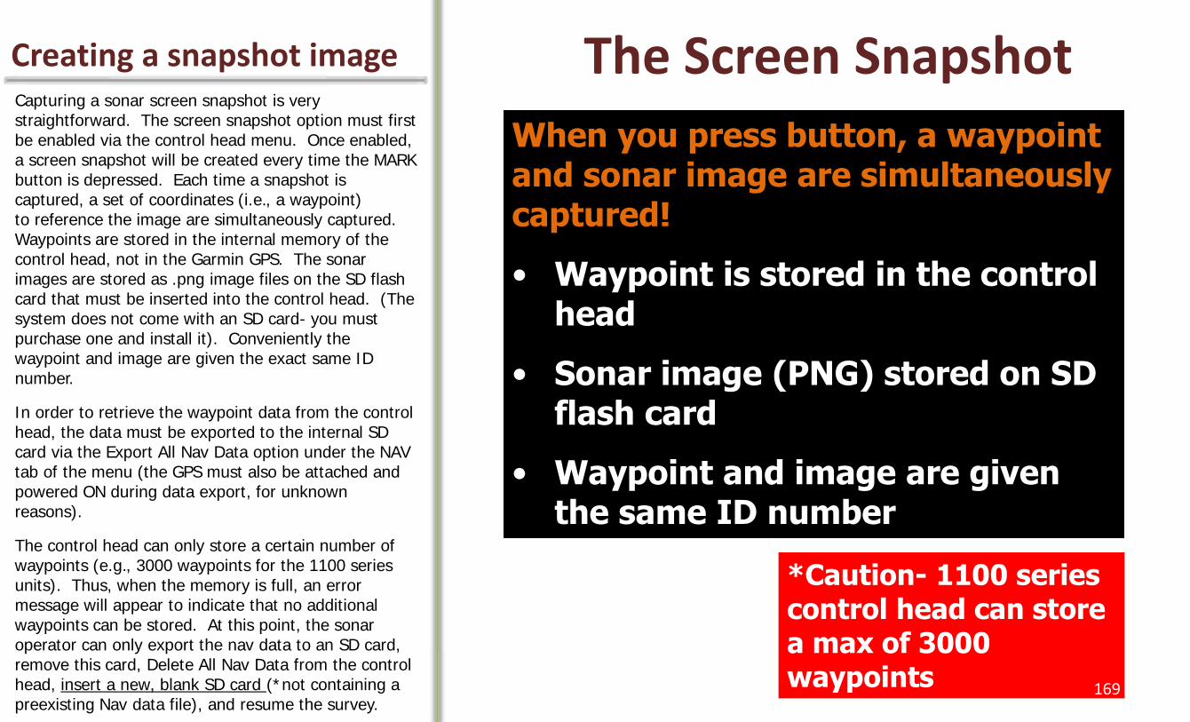
Creating a snapshot image The Screen Snapshot

When you press button, a waypoint and sonar image are simultaneously captured!

• Waypoint is stored in the control head

• Sonar image (PNG) stored on SD flash card

• Waypoint and image are given the same ID number

Capturing a sonar screen snapshot is very straightforward. The screen snapshot option must first be enabled via the control head menu. Once enabled, a screen snapshot will be created every time the MARK button is depressed. Each time a snapshot is captured, a set of coordinates (i.e., a waypoint) to reference the image are simultaneously captured. Waypoints are stored in the internal memory of the control head, not in the Garmin GPS. The sonar images are stored as .png image files on the SD flash card that must be inserted into the control head. (The system does not come with an SD card- you must purchase one and install it). Conveniently the waypoint and image are given the exact same ID number.

In order to retrieve the waypoint data from the control head, the data must be exported to the internal SD card via the Export All Nav Data option under the NAV tab of the menu (the GPS must also be attached and powered ON during data export, for unknown reasons).

The control head can only store a certain number of waypoints (e.g., 3000 waypoints for the 1100 series units). Thus, when the memory is full, an error message will appear to indicate that no additional waypoints can be stored. At this point, the sonar operator can only export the nav data to an SD card, remove this card, Delete All Nav Data from the control head, insert a new, blank SD card (*not containing a preexisting Nav data file), and resume the survey.

*Caution- 1100 series control head can store a max of 3000 waypoints 169

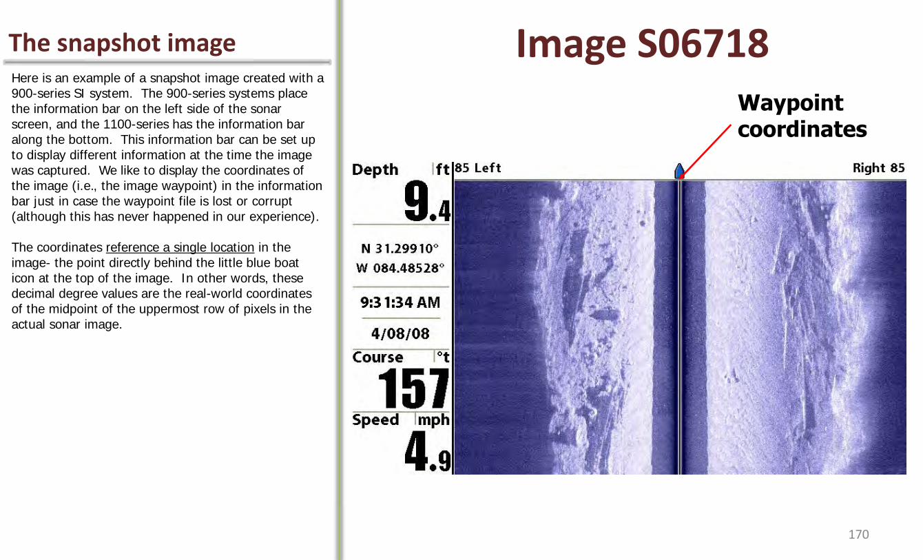
The snapshot image Image S06718 Here is an example of a snapshot image created with a 900-series SI system. The 900-series systems place the information bar on the left side of the sonar screen, and the 1100-series has the information bar along the bottom. This information bar can be set up to display different information at the time the image was captured. We like to display the coordinates of the image (i.e., the image waypoint) in the information bar just in case the waypoint file is lost or corrupt (although this has never happened in our experience). The coordinates reference a single location in the image- the point directly behind the little blue boat icon at the top of the image. In other words, these decimal degree values are the real-world coordinates of the midpoint of the uppermost row of pixels in the actual sonar image.

Waypoint coordinates

170

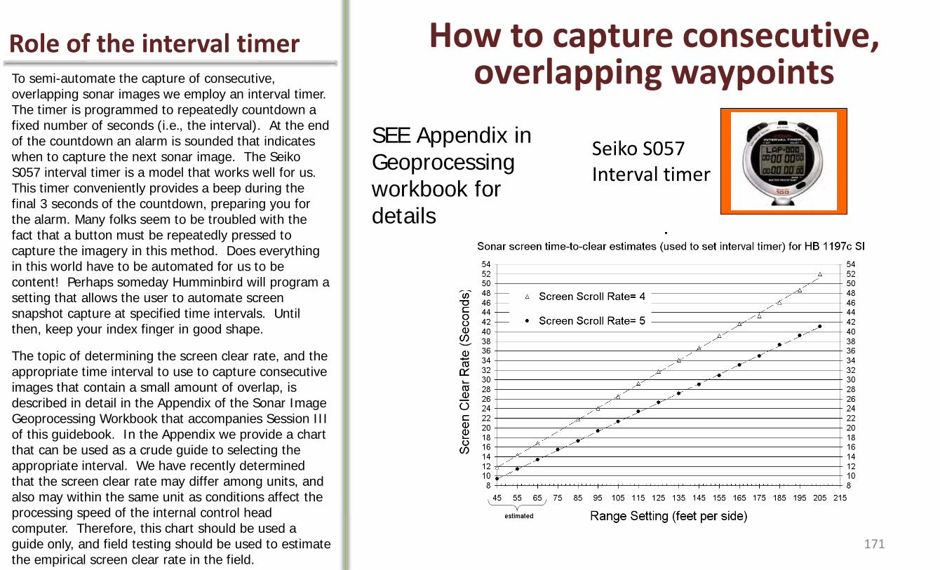
Role of the interval timer How to capture consecutive, overlapping waypoints

SEE Appendix in Geoprocessing workbook for details

Seiko S057 Interval timer

To semi-automate the capture of consecutive, overlapping sonar images we employ an interval timer. The timer is programmed to repeatedly countdown a fixed number of seconds (i.e., the interval). At the end of the countdown an alarm is sounded that indicates when to capture the next sonar image. The Seiko S057 interval timer is a model that works well for us. This timer conveniently provides a beep during the final 3 seconds of the countdown, preparing you for the alarm. Many folks seem to be troubled with the fact that a button must be repeatedly pressed to capture the imagery in this method. Does everything in this world have to be automated for us to be content! Perhaps someday Humminbird will program a setting that allows the user to automate screen snapshot capture at specified time intervals. Until then, keep your index finger in good shape.

The topic of determining the screen clear rate, and the appropriate time interval to use to capture consecutive images that contain a small amount of overlap, is described in detail in the Appendix of the Sonar Image Geoprocessing Workbook that accompanies Session III of this guidebook. In the Appendix we provide a chart that can be used as a crude guide to selecting the appropriate interval. We have recently determined that the screen clear rate may differ among units, and also may within the same unit as conditions affect the processing speed of the internal control head computer. Therefore, this chart should be used a guide only, and field testing should be used to estimate the empirical screen clear rate in the field.

171

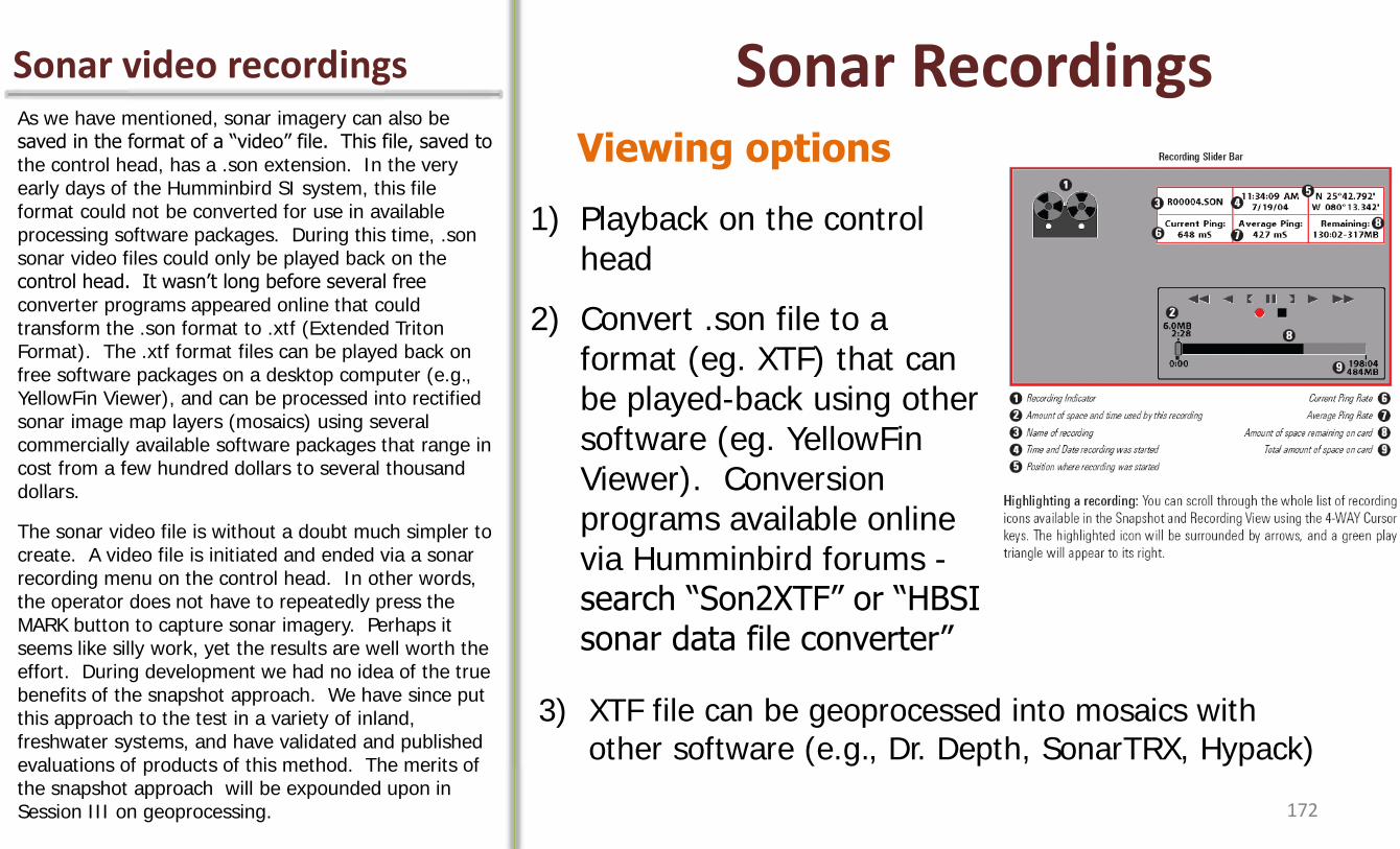
Sonar video recordings Sonar Recordings As we have mentioned, sonar imagery can also be saved in the format of a “video” file. This file, saved to the control head, has a .son extension. In the very early days of the Humminbird SI system, this file format could not be converted for use in available processing software packages. During this time, .son sonar video files could only be played back on the control head. It wasn’t long before several free converter programs appeared online that could transform the .son format to .xtf (Extended Triton Format). The .xtf format files can be played back on free software packages on a desktop computer (e.g., YellowFin Viewer), and can be processed into rectified sonar image map layers (mosaics) using several commercially available software packages that range in cost from a few hundred dollars to several thousand dollars.

The sonar video file is without a doubt much simpler to create. A video file is initiated and ended via a sonar recording menu on the control head. In other words, the operator does not have to repeatedly press the MARK button to capture sonar imagery. Perhaps it seems like silly work, yet the results are well worth the effort. During development we had no idea of the true benefits of the snapshot approach. We have since put this approach to the test in a variety of inland, freshwater systems, and have validated and published evaluations of products of this method. The merits of the snapshot approach will be expounded upon in Session III on geoprocessing.

1) Playback on the control head

2) Convert .son file to a format (eg. XTF) that can be played-back using other software (eg. YellowFin Viewer). Conversion programs available online via Humminbird forums - search “Son2XTF” or “HBSI sonar data file converter”

Viewing options

3) XTF file can be geoprocessed into mosaics with other software (e.g., Dr. Depth, SonarTRX, Hypack)

172

Media for data storage Memory Cards To save sonar screen snapshots, video recordings, or navigation data exported from the control head, you must purchase and install an SD memory card. The current screen snapshot file format is .png. These files are quite small, yet retain full image quality. A popular question is how many cards to carry and what size? Many sonar snapshots can be stored on a single 2 GB card. The likelihood of filling an empty 2 GB card with snapshots in 1 day is extremely low. We estimate that a 2 GB card could hold ~10 hours of continuously captured images (@ 3-second interval). We recommend that sonar operators carry 2 of these 2 GB cards with them on the water. The second card may come in handy if a dump of the waypoint data from the control head is necessary to free up internal memory on the device (this situation was discussed previously).

• Storing images requires an SD Memory Card

• How many cards should I carry?

2 2GB cards will store all images captured in 1 Day

173

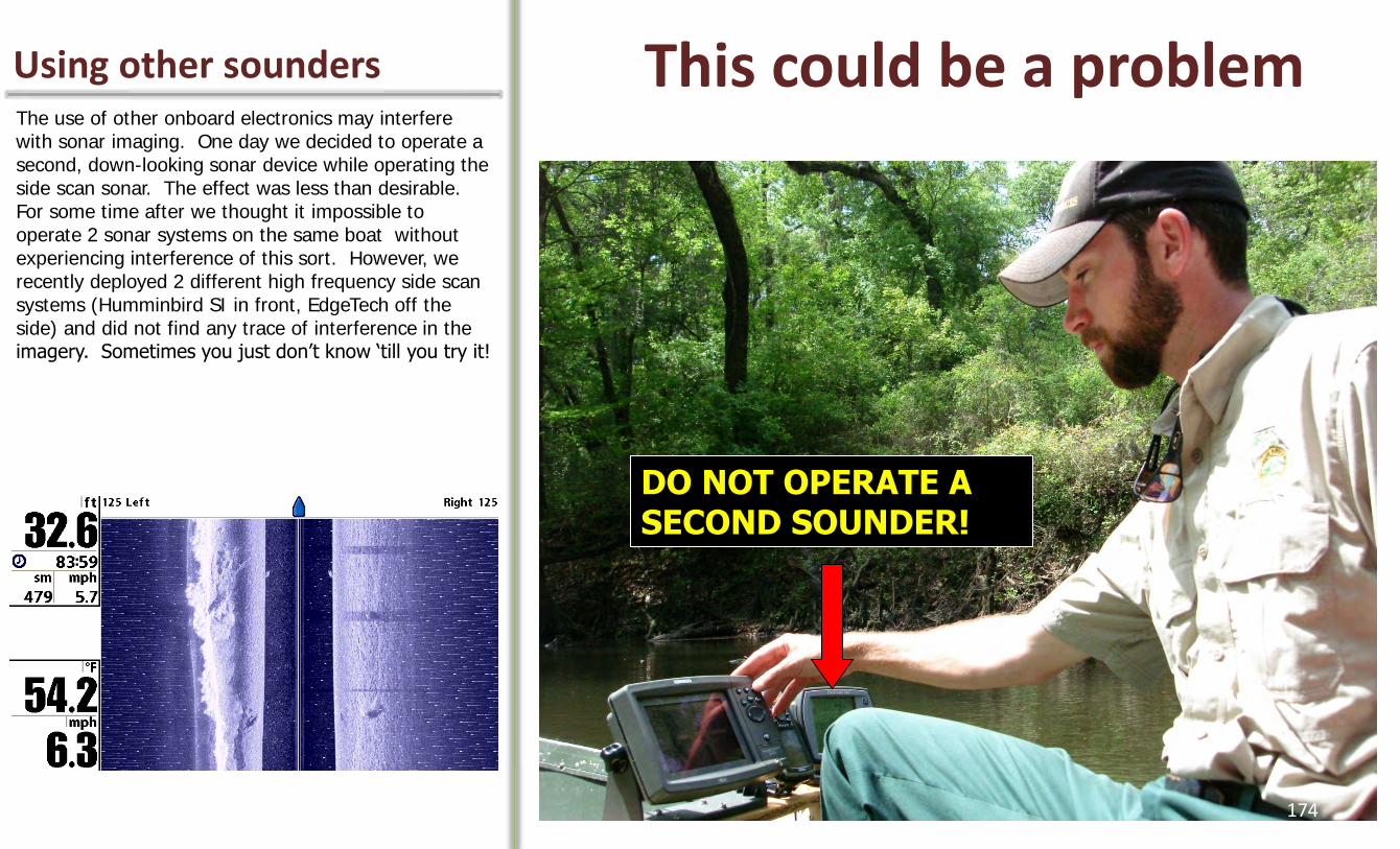
Using other sounders The use of other onboard electronics may interfere with sonar imaging. One day we decided to operate a second, down-looking sonar device while operating the side scan sonar. The effect was less than desirable. For some time after we thought it impossible to operate 2 sonar systems on the same boat without experiencing interference of this sort. However, we recently deployed 2 different high frequency side scan systems (Humminbird SI in front, EdgeTech off the side) and did not find any trace of interference in the imagery. Sometimes you just don’t know ‘till you try it!

This could be a problem

DO NOT OPERATE A SECOND SOUNDER!

174

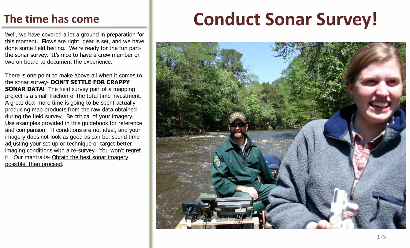
The time has come Well, we have covered a lot a ground in preparation for this moment. Flows are right, gear is set, and we have done some field testing. We’re ready for the fun part- the sonar survey. It’s nice to have a crew member or two on board to document the experience. There is one point to make above all when it comes to the sonar survey- DON’T SETTLE FOR CRAPPY SONAR DATA! The field survey part of a mapping project is a small fraction of the total time investment. A great deal more time is going to be spent actually producing map products from the raw data obtained during the field survey. Be critical of your imagery. Use examples provided in this guidebook for reference and comparison. If conditions are not ideal, and your imagery does not look as good as can be, spend time adjusting your set up or technique or target better imaging conditions with a re-survey. You won’t regret it. Our mantra is- Obtain the best sonar imagery possible, then proceed.

Conduct Sonar Survey!

175

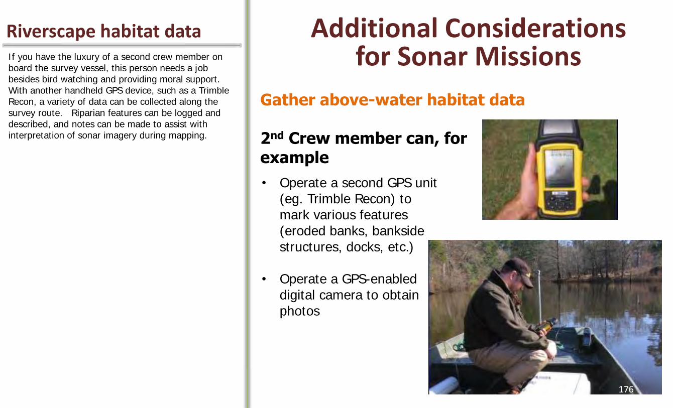
Riverscape habitat data Additional Considerations for Sonar Missions

Gather above-water habitat data 2nd Crew member can, for example

• Operate a second GPS unit (eg. Trimble Recon) to mark various features (eroded banks, bankside structures, docks, etc.)

• Operate a GPS-enabled digital camera to obtain photos

If you have the luxury of a second crew member on board the survey vessel, this person needs a job besides bird watching and providing moral support. With another handheld GPS device, such as a Trimble Recon, a variety of data can be collected along the survey route. Riparian features can be logged and described, and notes can be made to assist with interpretation of sonar imagery during mapping.

176

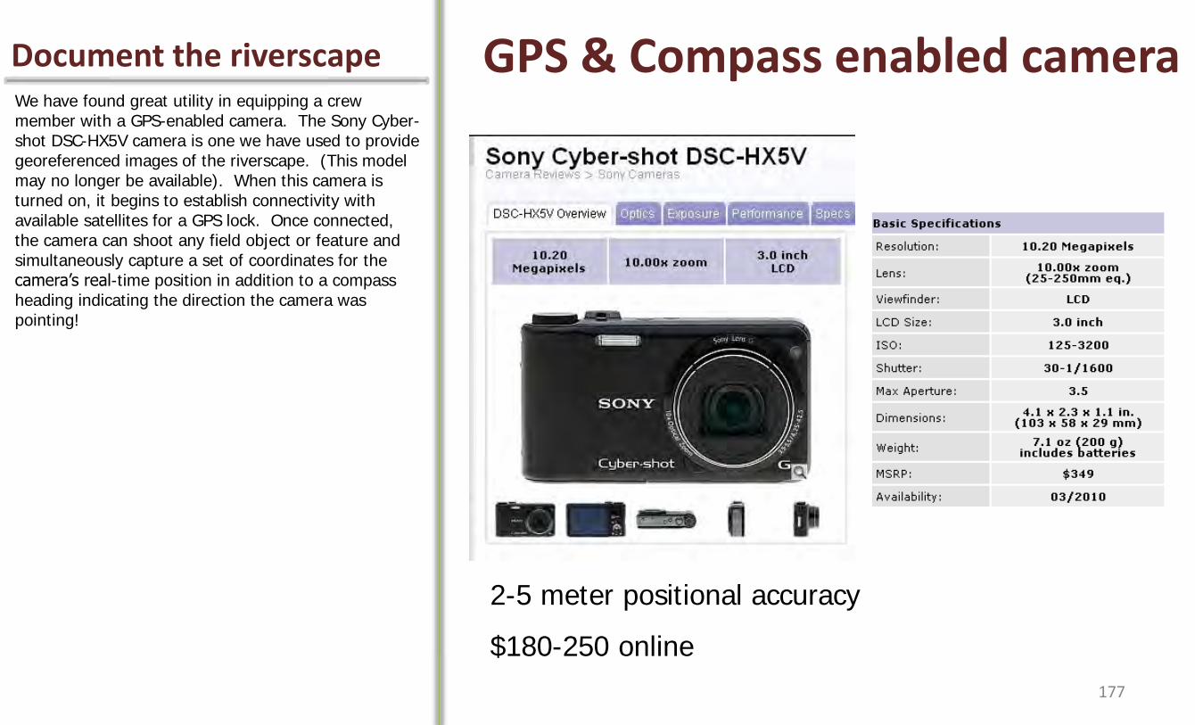
Document the riverscape GPS & Compass enabled camera We have found great utility in equipping a crew member with a GPS-enabled camera. The Sony Cyber-shot DSC-HX5V camera is one we have used to provide georeferenced images of the riverscape. (This model may no longer be available). When this camera is turned on, it begins to establish connectivity with available satellites for a GPS lock. Once connected, the camera can shoot any field object or feature and simultaneously capture a set of coordinates for the camera’s real-time position in addition to a compass heading indicating the direction the camera was pointing!

2-5 meter positional accuracy

$180-250 online

177

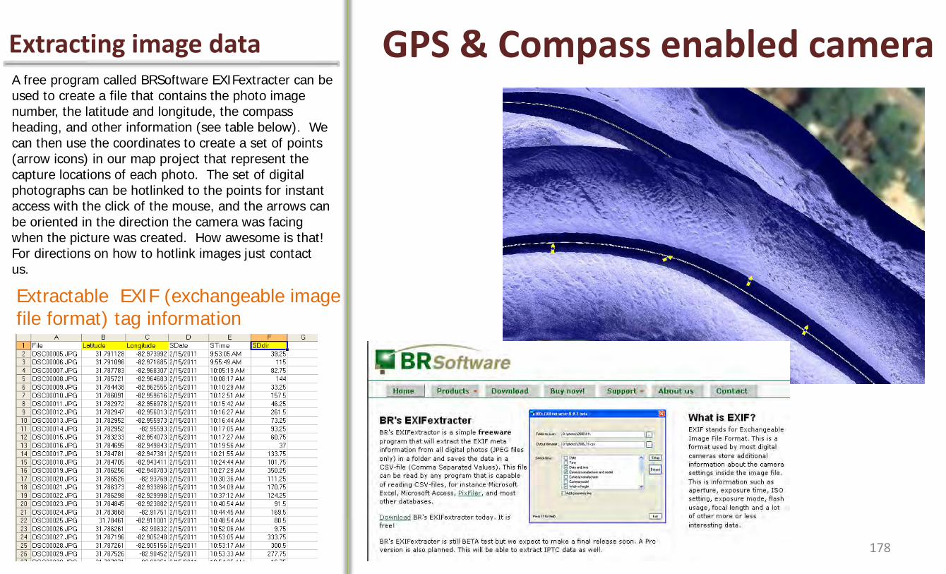
Extracting image data GPS & Compass enabled camera A free program called BRSoftware EXIFextracter can be used to create a file that contains the photo image number, the latitude and longitude, the compass heading, and other information (see table below). We can then use the coordinates to create a set of points (arrow icons) in our map project that represent the capture locations of each photo. The set of digital photographs can be hotlinked to the points for instant access with the click of the mouse, and the arrows can be oriented in the direction the camera was facing when the picture was created. How awesome is that! For directions on how to hotlink images just contact us.

Extractable EXIF (exchangeable image file format) tag information

178

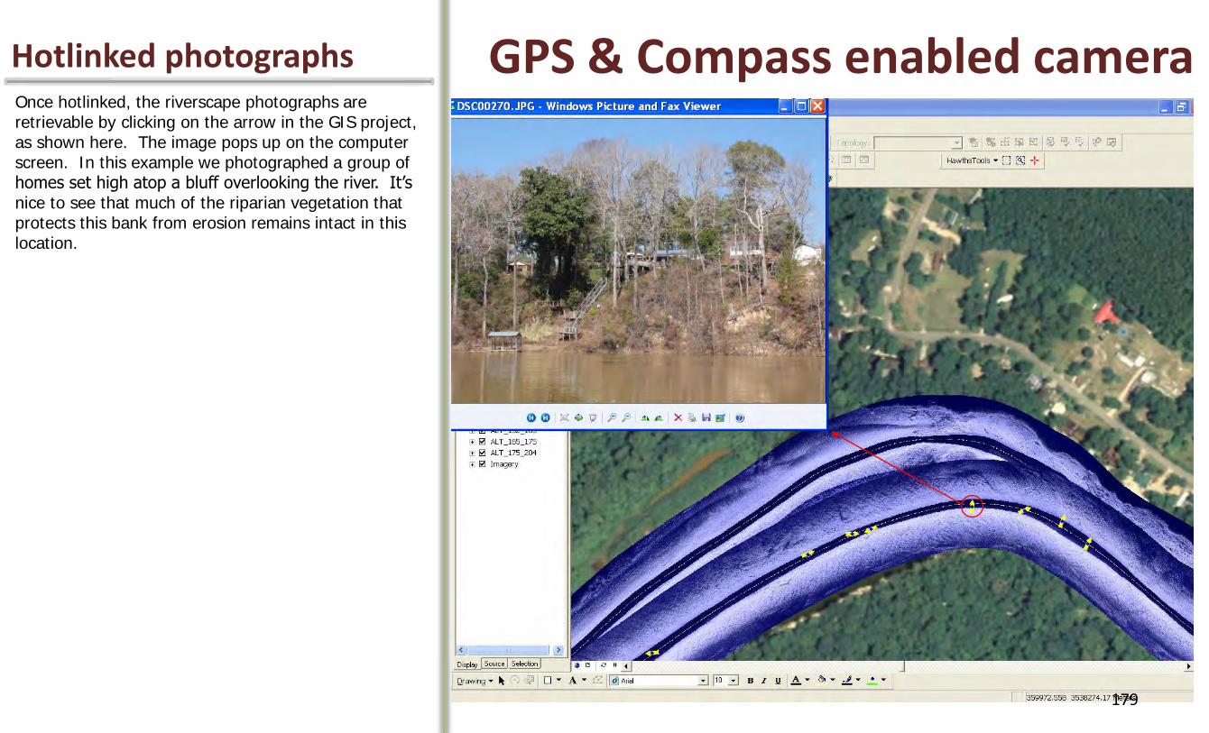
Hotlinked photographs GPS & Compass enabled camera Once hotlinked, the riverscape photographs are retrievable by clicking on the arrow in the GIS project, as shown here. The image pops up on the computer screen. In this example we photographed a group of homes set high atop a bluff overlooking the river. It’s nice to see that much of the riparian vegetation that protects this bank from erosion remains intact in this location.

179

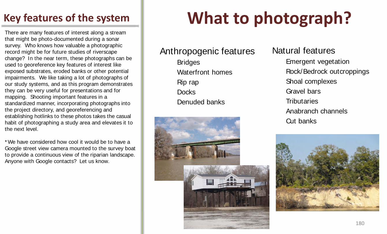
Key features of the system What to photograph? There are many features of interest along a stream that might be photo-documented during a sonar survey. Who knows how valuable a photographic record might be for future studies of riverscape change? In the near term, these photographs can be used to georeference key features of interest like exposed substrates, eroded banks or other potential impairments. We like taking a lot of photographs of our study systems, and as this program demonstrates they can be very useful for presentations and for mapping. Shooting important features in a standardized manner, incorporating photographs into the project directory, and georeferencing and establishing hotlinks to these photos takes the casual habit of photographing a study area and elevates it to the next level. *We have considered how cool it would be to have a Google street view camera mounted to the survey boat to provide a continuous view of the riparian landscape. Anyone with Google contacts? Let us know.

Anthropogenic features Bridges

Waterfront homes

Rip rap

Docks

Denuded banks

Natural features Emergent vegetation

Rock/Bedrock outcroppings

Shoal complexes

Gravel bars

Tributaries

Anabranch channels

Cut banks

180

Transferring Data Hardware/Software for Data Transfer Back in the days of the original 981c, to download data

you needed something called the PC Connect Kit to power the control head with two 9-volt batteries while connected to a desktop computer for a data dump. The 9-volts never lasted long, and the data transfer process often failed for unknown reasons. Data download is so easy now. You will need a program called HumminbirdPC. This program is free, and can be downloaded from Humminbird once you register your unit. Registration creates an online user account that can be checked for software updates and the like. (Registration is thus something we highly recommend). To transfer waypoint data from the control head to the SD card, you will need to execute the Export All Nav Data option found under the Nav menu in the field prior to powering down the control head and GPS. The SD card will now contain your sonar images (in the SNAPSHOT folder) and the waypoint data (a DATA.HWR file in the MATRIX folder). You then remove the SD card from the control head and insert it into your work computer. Launch the HumminbirdPC program and select the Download from SD/MMC to PC arrow under the card icon. Each time a file is downloaded, HumminbirdPC automatically saves a copy of this .gpx file to a folder, but we like to save a copy into our project directory as well. Expand the directory for this file in the menu of HumminbirdPC, and click on the waypoints tab. A table of waypoint data will appear; select, copy, and paste the data from this table into a new Excel spreadsheet.

• PC Connect Accessory Kit sold by Humminbird ($24), not needed to transfer data from 998c or 1198c HSI

• HumminbirdPC software (free from Humminbird), available upon registering your unit

• Memory Card Reader (USB port connection)

PC Connect Kit needed if using 981c only

181

Transferring Data Data Transfer The steps following the transfer of the waypoint data from HumminbirdPC to an Excel spreadsheet are detailed in the Sonar Imagery Geoprocessing Workbook. This workbook explains how to prepare the data for import into a new ArcGIS project, and what to do following importation.

Detailed instructions on how to transfer the 3 survey data sets to a desktop computer are provided in the Sonar Imagery Geoprocessing Workbook

182

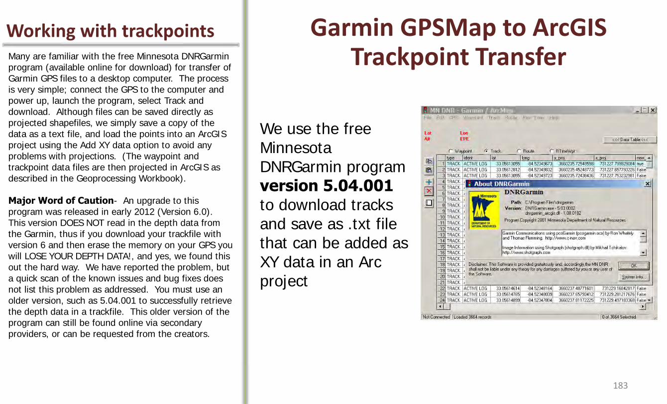
Working with trackpoints Garmin GPSMap to ArcGIS Trackpoint Transfer Many are familiar with the free Minnesota DNRGarmin

program (available online for download) for transfer of Garmin GPS files to a desktop computer. The process is very simple; connect the GPS to the computer and power up, launch the program, select Track and download. Although files can be saved directly as projected shapefiles, we simply save a copy of the data as a text file, and load the points into an ArcGIS project using the Add XY data option to avoid any problems with projections. (The waypoint and trackpoint data files are then projected in ArcGIS as described in the Geoprocessing Workbook). Major Word of Caution- An upgrade to this program was released in early 2012 (Version 6.0). This version DOES NOT read in the depth data from the Garmin, thus if you download your trackfile with version 6 and then erase the memory on your GPS you will LOSE YOUR DEPTH DATA!, and yes, we found this out the hard way. We have reported the problem, but a quick scan of the known issues and bug fixes does not list this problem as addressed. You must use an older version, such as 5.04.001 to successfully retrieve the depth data in a trackfile. This older version of the program can still be found online via secondary providers, or can be requested from the creators.

We use the free Minnesota DNRGarmin program version 5.04.001 to download tracks and save as .txt file that can be added as XY data in an Arc project

183

Transferring images Sonar Image Transfer Image transfer is as easy as can be. Insert the SD card into a desktop computer and copy the contents of the SNAPSHOT folder (or a subset of the contents representing only the survey images of interest) to a folder in the project directory for raw sonar images. The geoprocessing workbook describes our preferred method for organization of survey data using a structured, hierarchical directory for each sonar mapping project. In order to successfully use the custom sonar tools created by Thom Litts for image processing, elements of your project directory must exactly match the directory structure we describe in the workbook. Thus, it’s a good idea at this point to begin reading the introductory sections of this workbook in preparation for the next session. This concludes Session II- Part B, The Sonar Mission. We’re now ready to turn our attention to processing all of the raw sonar data we have transferred to our work computer into beautiful sonar image map layers.

184

Session III Geoprocessing (Placeholder)

185

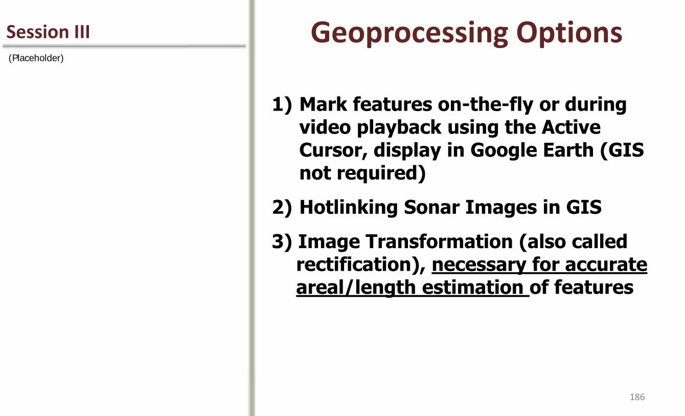
Session III Geoprocessing Options (Placeholder)

1) Mark features on-the-fly or during video playback using the Active Cursor, display in Google Earth (GIS not required)

2) Hotlinking Sonar Images in GIS

3) Image Transformation (also called rectification), necessary for accurate areal/length estimation of features

186

The sonar cursor 1) Marking features with the sonar cursor (Placeholder)

187

Viewing in Google Earth 1) Marking features with cursor (Placeholder)

188

What is hotlinking? 2) Hotlinking images (Placeholder)

Hotlinking:

• Procedure that establishes a connection within a GIS framework between a waypoint and an associated image (waypoint and image have same ID #)

• Enables quick access to the image via point-n-click

• Represents a first-step towards proper geo-positioning of image related habitat info

189

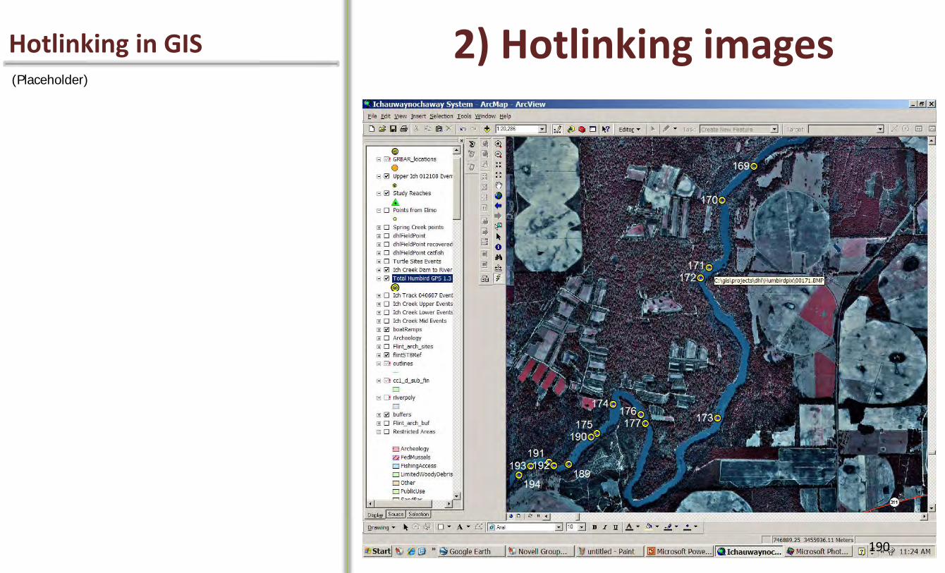
2) Hotlinking images (Placeholder)

Hotlinking in GIS

190

Point and click 2) Hotlinking images (Placeholder)

191

Image rectification 3) Image Transformation (Placeholder)

Via our method… uses images and coordinate data captured via the “Sonar Snapshot” approach, …and software tools and techniques we have developed. The process involves the following steps:

192

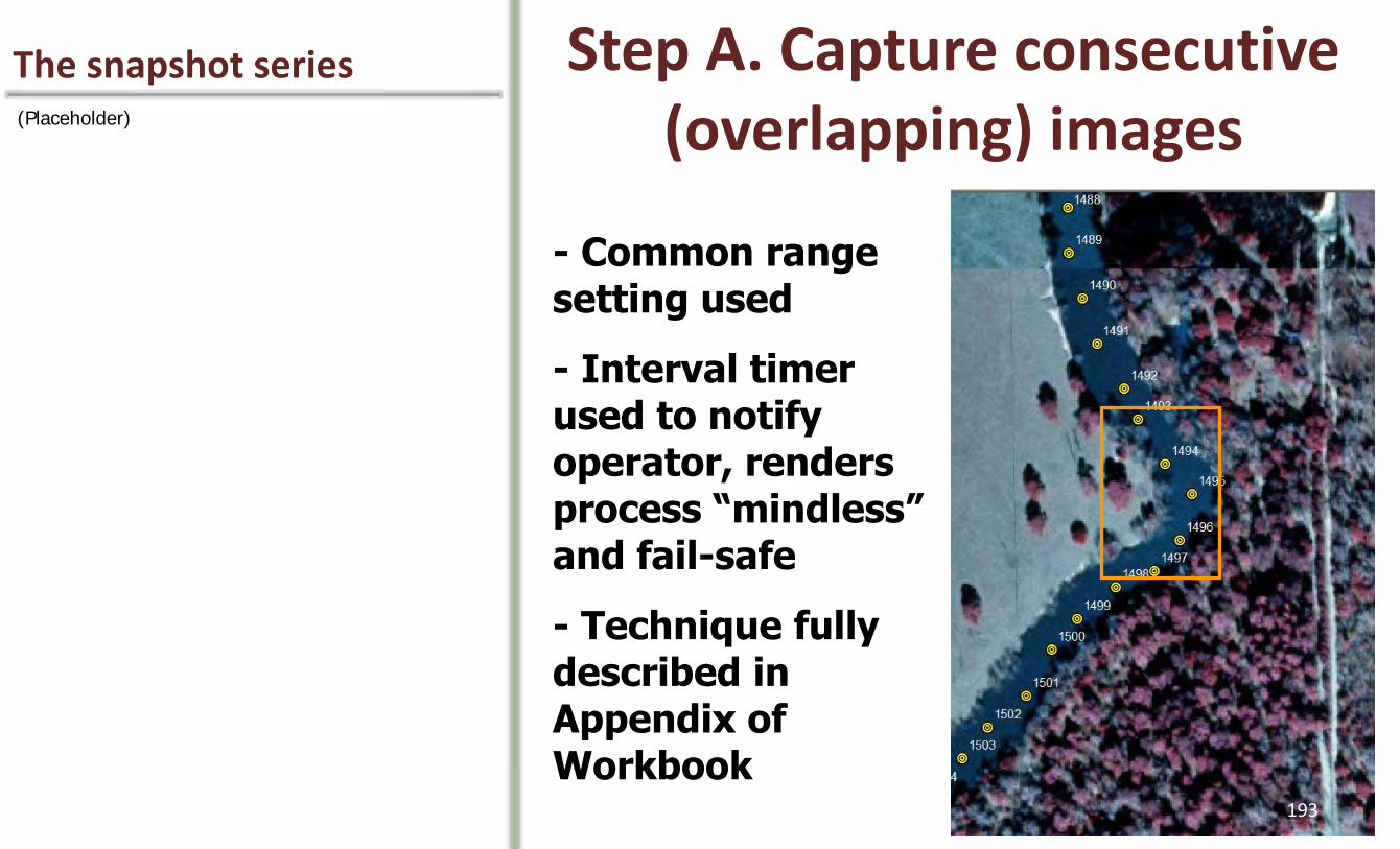
The snapshot series Step A. Capture consecutive (overlapping) images (Placeholder)

- Common range setting used

- Interval timer used to notify operator, renders process “mindless” and fail-safe

- Technique fully described in Appendix of Workbook 193

Next steps Step B. Data Preparation (Placeholder)

1. Import, clean, organize, and process GPS data (ArcGIS/ETGeowizards)

2. Subset Images – collar removal (IrfanView / Batch processing)

3. Image matching – identify overlap (clip) (ArcGIS)

Step C. Control Point Generation

Step D. Rectification and Mosaicking

194

Organize segment data Step B1. Import, Organize Data (Placeholder)

• During sonar surveys, breaks in the consecutive, overlapping image series are inevitable

• Breaks occur whenever a survey run is stopped or paused (eg. lunch break), or whenever the range setting is changed

• You must organize data sets into discrete processing segments based these break points (field notes help)

• This is done by creating folders for each segment and moving appropriate GPS and raster data into segment folders

• All GPS and image processing steps are then performed on each segment data set

Organizing data into processing segments

Import GPS waypoints and tracks 195

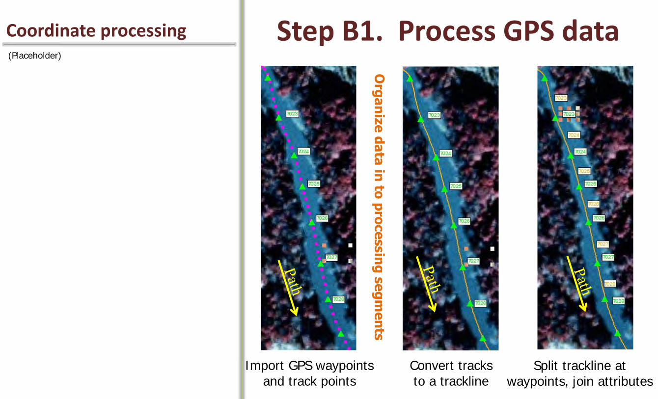
Coordinate processing Step B1. Process GPS data (Placeholder)

Import GPS waypoints and track points

Convert tracks to a trackline

Split trackline at waypoints, join attributes

Org

an

ize

da

ta in

to p

roce

ssin

g s

eg

me

nts

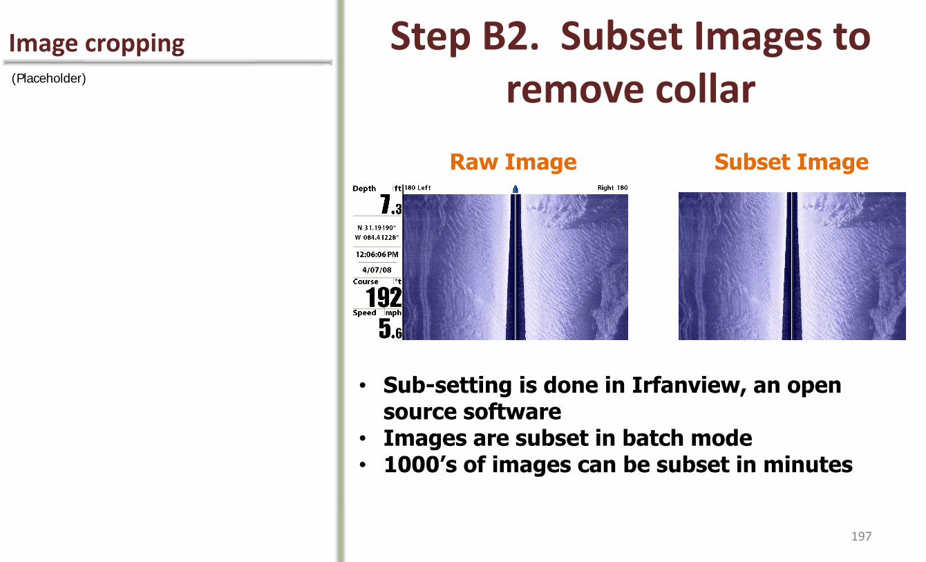
Image cropping Step B2. Subset Images to remove collar (Placeholder)

Raw Image Subset Image

• Sub-setting is done in Irfanview, an open source software

• Images are subset in batch mode • 1000’s of images can be subset in minutes

197

Image clipping Step B3. Image Matching (clip) (Placeholder)

198

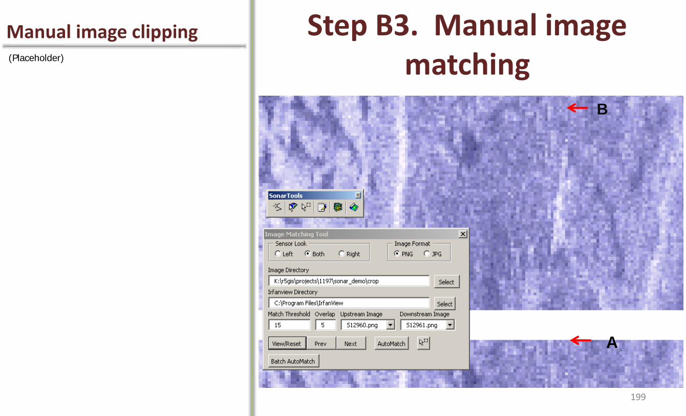
Manual image clipping Step B3. Manual image matching (Placeholder)

A

B

199

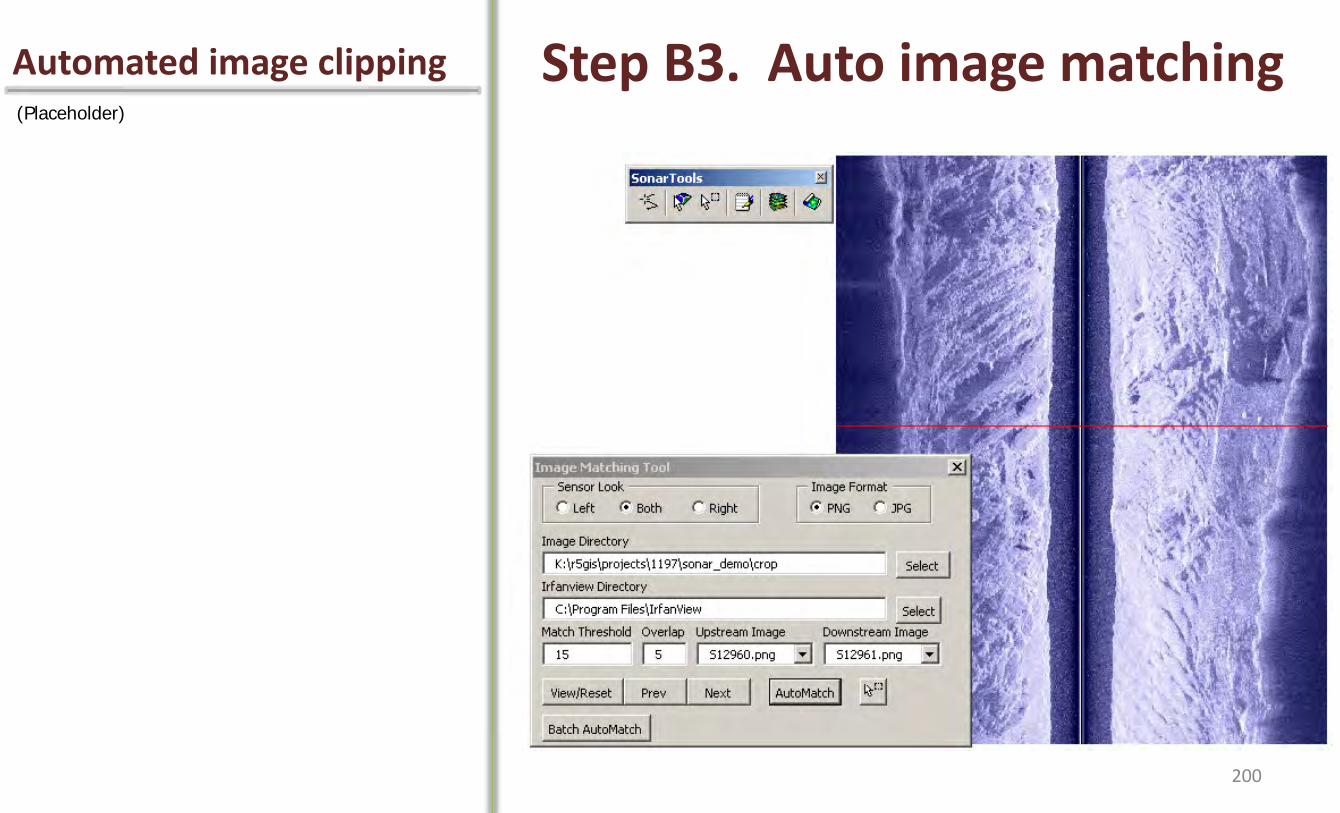
Automated image clipping Step B3. Auto image matching (Placeholder)

200

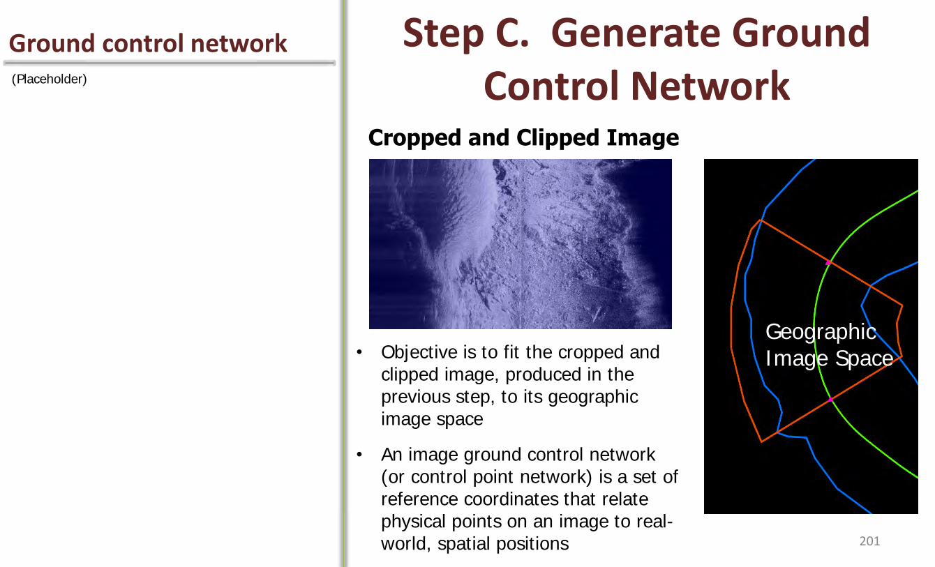
Ground control network Step C. Generate Ground Control Network (Placeholder)

Cropped and Clipped Image

Geographic Image Space • Objective is to fit the cropped and

clipped image, produced in the previous step, to its geographic image space

• An image ground control network (or control point network) is a set of reference coordinates that relate physical points on an image to real-world, spatial positions 201

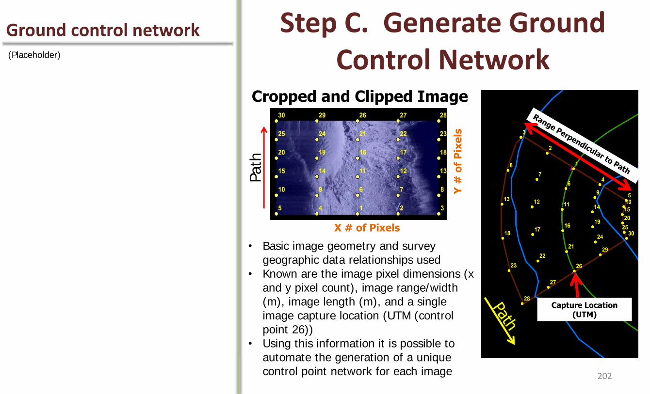
Ground control network Step C. Generate Ground Control Network (Placeholder)


• Basic image geometry and survey geographic data relationships used

• Known are the image pixel dimensions (x and y pixel count), image range/width (m), image length (m), and a single image capture location (UTM (control point 26))

• Using this information it is possible to automate the generation of a unique control point network for each image

Path

X # of Pixels

Y #

of

Pix

els

Capture Location (UTM)

202

Transformation of image Step D. Image Rectification (Placeholder)


When each image has a control point network, images can be transformed (or rectified) from image space into geographic space

Path

203

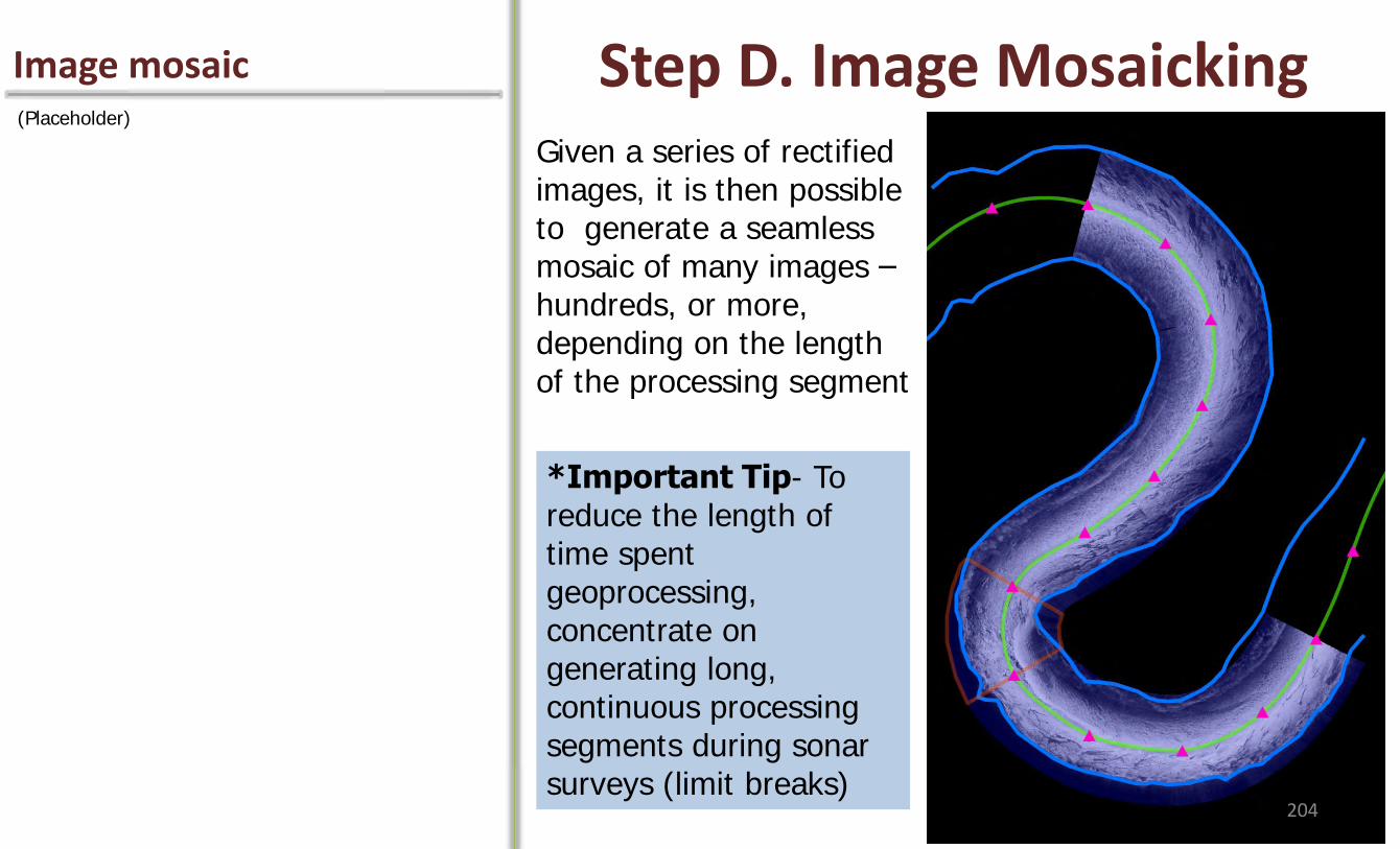
Image mosaic Step D. Image Mosaicking (Placeholder)

Given a series of rectified images, it is then possible to generate a seamless mosaic of many images – hundreds, or more, depending on the length of the processing segment

*Important Tip- To reduce the length of time spent geoprocessing, concentrate on generating long, continuous processing segments during sonar surveys (limit breaks)

204

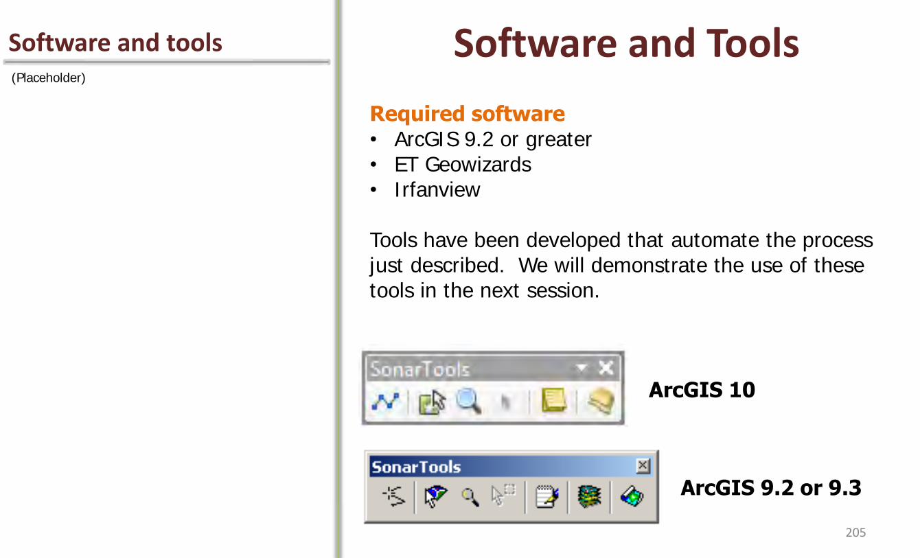
Software and tools Software and Tools (Placeholder)

Required software • ArcGIS 9.2 or greater • ET Geowizards • Irfanview

Tools have been developed that automate the process just described. We will demonstrate the use of these tools in the next session.

ArcGIS 9.2 or 9.3

ArcGIS 10

205

Rectification problems Warping and Rectification Failures (Placeholder)

What to do if an image fails to rectify?

How to fix warped images?

How can I avoid warping?

206

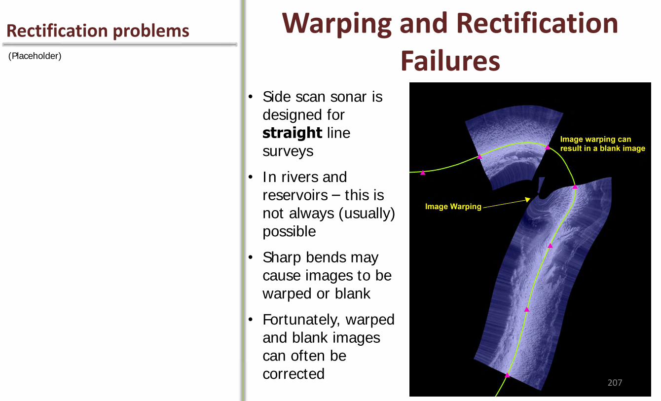
Rectification problems Warping and Rectification Failures (Placeholder)

• Side scan sonar is designed for straight line surveys

• In rivers and reservoirs – this is not always (usually) possible

• Sharp bends may cause images to be warped or blank

• Fortunately, warped and blank images can often be corrected

207

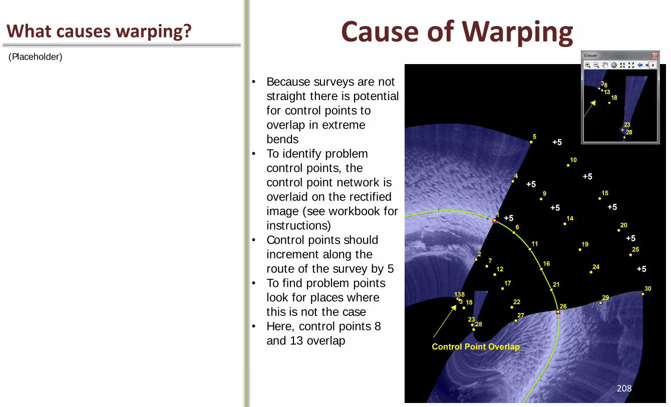
What causes warping? Cause of Warping (Placeholder)

• Because surveys are not straight there is potential for control points to overlap in extreme bends

• To identify problem control points, the control point network is overlaid on the rectified image (see workbook for instructions)

• Control points should increment along the route of the survey by 5

• To find problem points look for places where this is not the case

• Here, control points 8 and 13 overlap

208

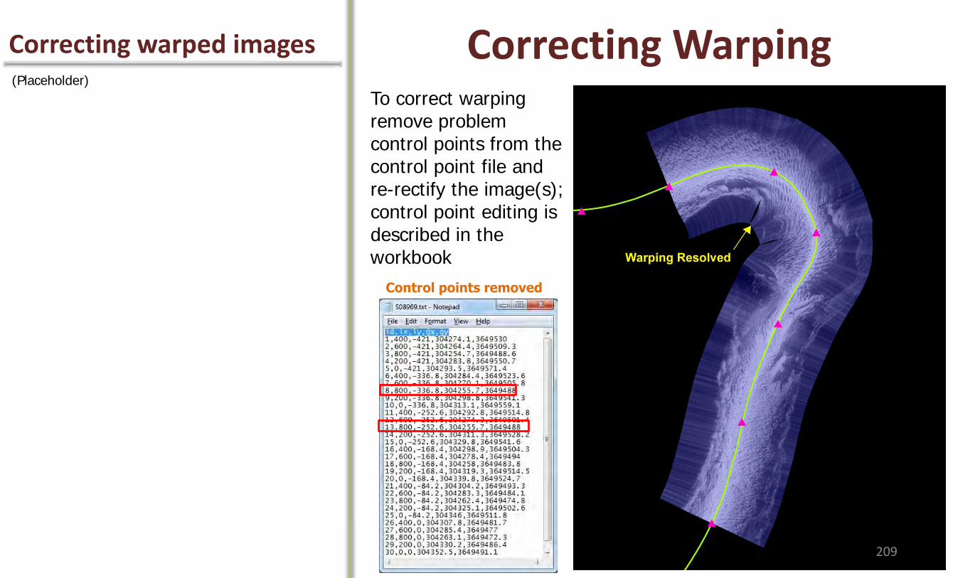
Correcting warped images Correcting Warping (Placeholder)

Control points removed

To correct warping remove problem control points from the control point file and re-rectify the image(s); control point editing is described in the workbook

209

How to avoid warping Preventing Warping (Placeholder)

Supplemental image capture during survey to preempt warping (theoretical)

210

Sonar video files Snapshot vs. Video Approaches As mentioned early in the program, several free programs are now available that convert the .son sonar video recording file format to the .xtf format that can be processed by commercially available software packages. Softwares vary considerably in price, from hundreds to thousands of dollars. Given our early success with the development of the snapshot approach, we have only spent a bit of time examining a few of the software packages available for Humminbird sonar video file processing. We have long discussed the idea of conducting a more rigorous evaluation of processing methodologies, but have not yet found the time to do so. Done properly, an assessment could provide a lot of useful information to users who are deciding which image capture and processing option to pursue. Several important factors that should be evaluated include: time demands and cost, end-product image quality/resolution, and overall performance in sub-optimal scanning environments such as in narrow canopied streams, or along tortuous (i.e, highly sinuous) routes.

• HSI video file .son to .xtf conversion tools now available (e.g., son2xtf program)

• Processing Humminbird video files

converted to .xtf now possible via 3rd party, commercially available software packages

Examples- Hypack ($4300), Dr. Depth ($225), SonarTRX ($90 Humminbird version, 130$ xtf)

211

Snapshot processing Our Method

212

Although our evaluations are limited, the following three slides provide an singular example for comparing the output from two different video processing softwares to the snapshot approach output (shown here in this slide). This processed image represents a scan of the right bank of a short reach of the Apalachicola River. The imagery is not very detailed in this reach, yet some of the differences in bedform (ripples, dunes, and plane bed) can be seen, in addition to the stippled signature of the partially submerged, bank-side willow stands (upper right and left sides of image).

Video processing Hypack Hypack is a commercially available software package that is capable of doing a lot more than just processing Humminbird .son files, but costs range in the thousands of dollars. This image example was not processed by us, but rather by a Hypack representative who was provided the file. The imagery from this example was captured on a different day, thus bedforms may have changed to some degree. Nevertheless, some differences in overall image quality are evident.

213

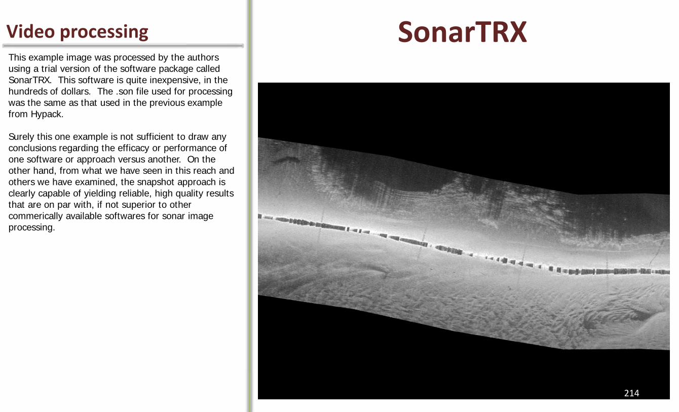
Video processing SonarTRX This example image was processed by the authors using a trial version of the software package called SonarTRX. This software is quite inexpensive, in the hundreds of dollars. The .son file used for processing was the same as that used in the previous example from Hypack. Surely this one example is not sufficient to draw any conclusions regarding the efficacy or performance of one software or approach versus another. On the other hand, from what we have seen in this reach and others we have examined, the snapshot approach is clearly capable of yielding reliable, high quality results that are on par with, if not superior to other commerically available softwares for sonar image processing.

214

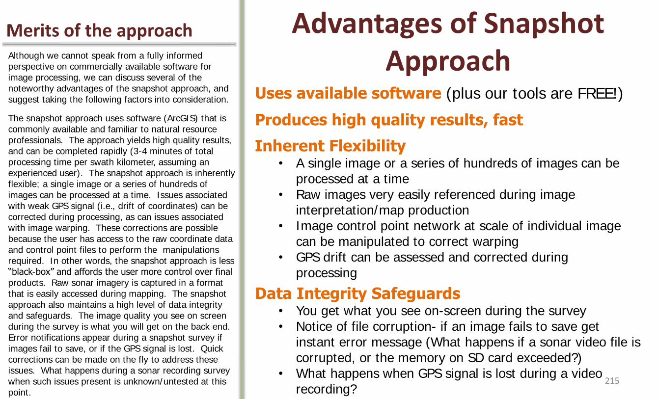
Merits of the approach Advantages of Snapshot Approach Although we cannot speak from a fully informed

perspective on commercially available software for image processing, we can discuss several of the noteworthy advantages of the snapshot approach, and suggest taking the following factors into consideration.

The snapshot approach uses software (ArcGIS) that is commonly available and familiar to natural resource professionals. The approach yields high quality results, and can be completed rapidly (3-4 minutes of total processing time per swath kilometer, assuming an experienced user). The snapshot approach is inherently flexible; a single image or a series of hundreds of images can be processed at a time. Issues associated with weak GPS signal (i.e., drift of coordinates) can be corrected during processing, as can issues associated with image warping. These corrections are possible because the user has access to the raw coordinate data and control point files to perform the manipulations required. In other words, the snapshot approach is less “black-box” and affords the user more control over final products. Raw sonar imagery is captured in a format that is easily accessed during mapping. The snapshot approach also maintains a high level of data integrity and safeguards. The image quality you see on screen during the survey is what you will get on the back end. Error notifications appear during a snapshot survey if images fail to save, or if the GPS signal is lost. Quick corrections can be made on the fly to address these issues. What happens during a sonar recording survey when such issues present is unknown/untested at this point.

Inherent Flexibility • A single image or a series of hundreds of images can be

processed at a time • Raw images very easily referenced during image

interpretation/map production • Image control point network at scale of individual image

can be manipulated to correct warping • GPS drift can be assessed and corrected during

processing

Data Integrity Safeguards • You get what you see on-screen during the survey • Notice of file corruption- if an image fails to save get

instant error message (What happens if a sonar video file is corrupted, or the memory on SD card exceeded?)

• What happens when GPS signal is lost during a video recording?

Uses available software (plus our tools are FREE!)

Produces high quality results, fast

215

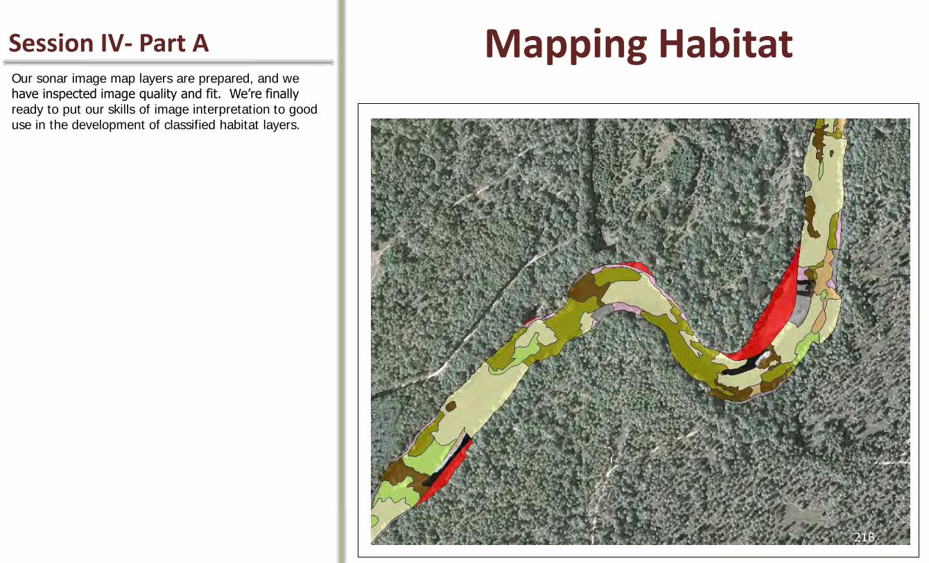
Session IV- Part A Mapping Habitat Our sonar image map layers are prepared, and we have inspected image quality and fit. We’re finally ready to put our skills of image interpretation to good use in the development of classified habitat layers.

216

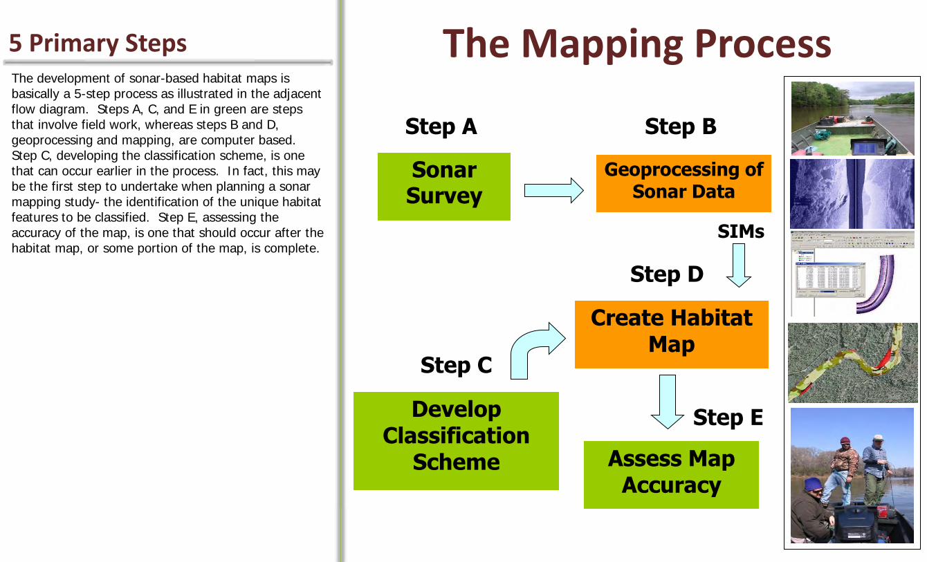
5 Primary Steps The Mapping Process The development of sonar-based habitat maps is basically a 5-step process as illustrated in the adjacent flow diagram. Steps A, C, and E in green are steps that involve field work, whereas steps B and D, geoprocessing and mapping, are computer based. Step C, developing the classification scheme, is one that can occur earlier in the process. In fact, this may be the first step to undertake when planning a sonar mapping study- the identification of the unique habitat features to be classified. Step E, assessing the accuracy of the map, is one that should occur after the habitat map, or some portion of the map, is complete.

Sonar Survey

Step A

Geoprocessing of Sonar Data

Step B

Step C

Develop Classification

Scheme Assess Map Accuracy

Step E

Create Habitat Map

Step D

SIMs

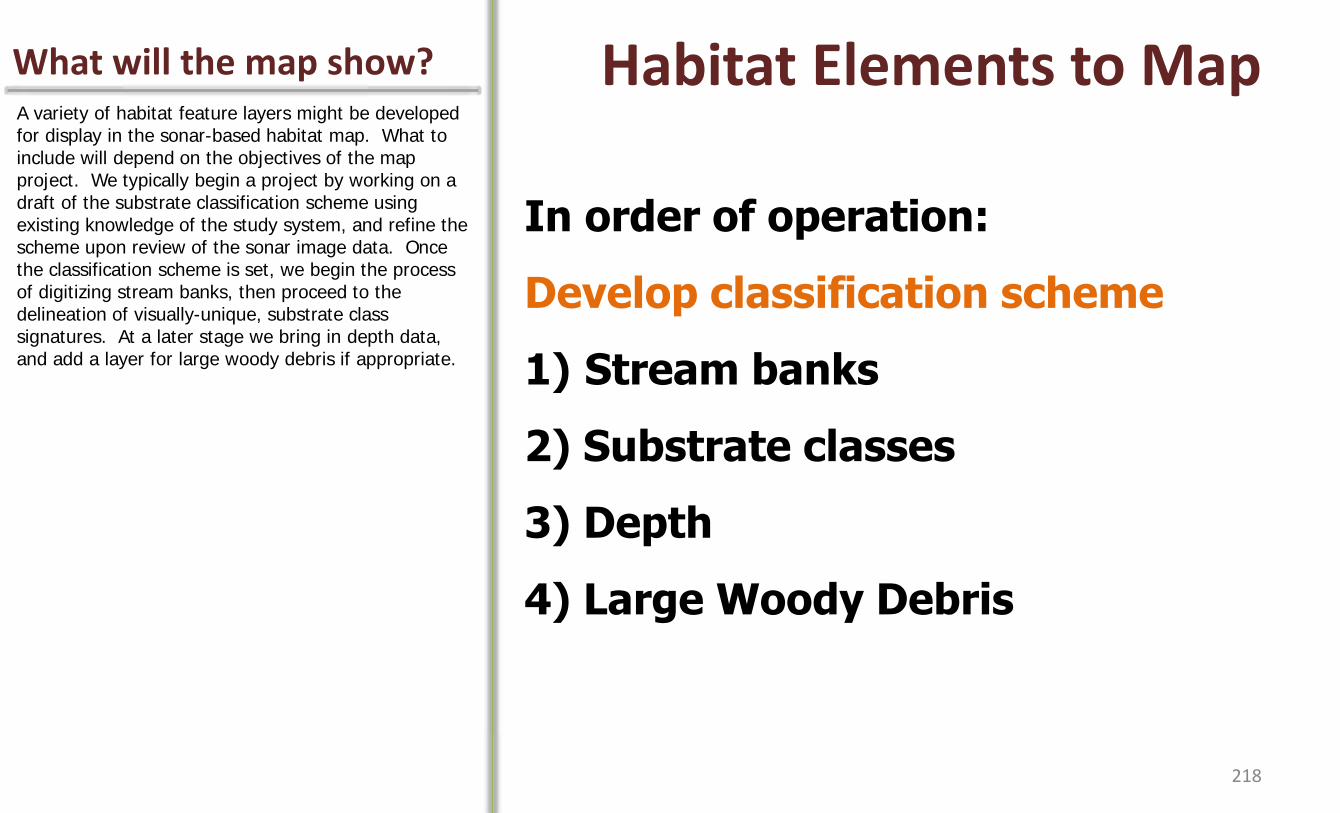
What will the map show? Habitat Elements to Map A variety of habitat feature layers might be developed for display in the sonar-based habitat map. What to include will depend on the objectives of the map project. We typically begin a project by working on a draft of the substrate classification scheme using existing knowledge of the study system, and refine the scheme upon review of the sonar image data. Once the classification scheme is set, we begin the process of digitizing stream banks, then proceed to the delineation of visually-unique, substrate class signatures. At a later stage we bring in depth data, and add a layer for large woody debris if appropriate.

1) Stream banks

In order of operation:

Develop classification scheme

1) Stream banks

2) Substrate classes

3) Depth

4) Large Woody Debris

218

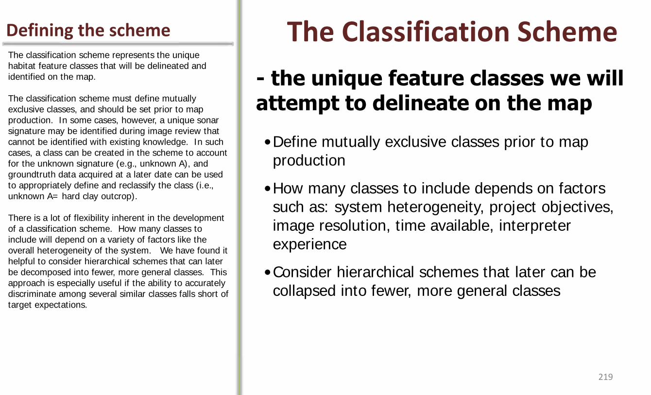
Defining the scheme The Classification Scheme The classification scheme represents the unique habitat feature classes that will be delineated and identified on the map. The classification scheme must define mutually exclusive classes, and should be set prior to map production. In some cases, however, a unique sonar signature may be identified during image review that cannot be identified with existing knowledge. In such cases, a class can be created in the scheme to account for the unknown signature (e.g., unknown A), and groundtruth data acquired at a later date can be used to appropriately define and reclassify the class (i.e., unknown A= hard clay outcrop). There is a lot of flexibility inherent in the development of a classification scheme. How many classes to include will depend on a variety of factors like the overall heterogeneity of the system. We have found it helpful to consider hierarchical schemes that can later be decomposed into fewer, more general classes. This approach is especially useful if the ability to accurately discriminate among several similar classes falls short of target expectations.

- the unique feature classes we will attempt to delineate on the map

•Define mutually exclusive classes prior to map production

•How many classes to include depends on factors such as: system heterogeneity, project objectives, image resolution, time available, interpreter experience

•Consider hierarchical schemes that later can be collapsed into fewer, more general classes

219

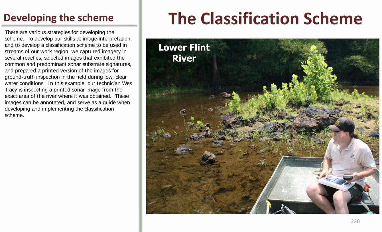
Developing the scheme The Classification Scheme There are various strategies for developing the scheme. To develop our skills at image interpretation, and to develop a classification scheme to be used in streams of our work region, we captured imagery in several reaches, selected images that exhibited the common and predominant sonar substrate signatures, and prepared a printed version of the images for ground-truth inspection in the field during low, clear water conditions. In this example, our technician Wes Tracy is inspecting a printed sonar image from the exact area of the river where it was obtained. These images can be annotated, and serve as a guide when developing and implementing the classification scheme.

1) Stream banks

Lower Flint River

220

S

Rf Rf

Rb

VB

Washing Machine & LWD

Developing the scheme Inspecting Sonar Images

Printed images are annotated in field

Here is an example of a printed sonar image that was annotated in the field during a groundtruthing expedition. The codes refer to classes in the scheme (e.g., Rb= Rocky boulder). In this case, we delineated an area of vegetated bank in the upper left corner of the image. This class did not appear in the final scheme as it was either very rare, or the vegetation itself did not exist at the time of the sonar survey. We also happened to find a washing machine among some logs in this reach.

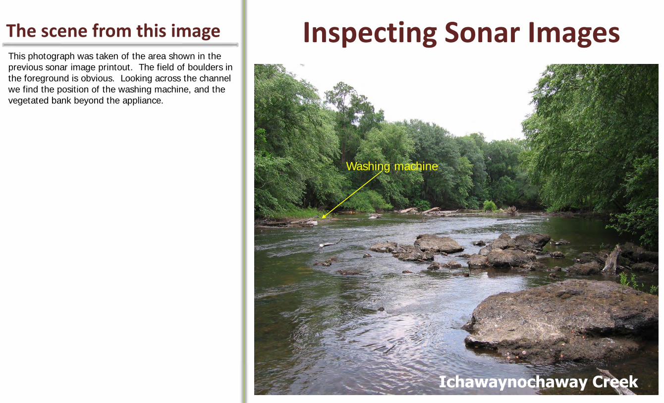
The scene from this image Inspecting Sonar Images This photograph was taken of the area shown in the previous sonar image printout. The field of boulders in the foreground is obvious. Looking across the channel we find the position of the washing machine, and the vegetated bank beyond the appliance.

Washing machine


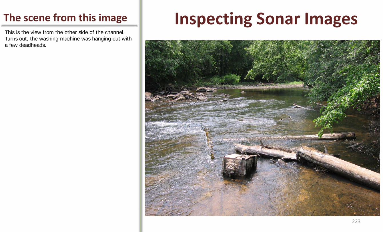
The scene from this image Inspecting Sonar Images This is the view from the other side of the channel. Turns out, the washing machine was hanging out with a few deadheads.

223

What is the MMU? Minimum Map Unit (MMU) Along with the classification scheme, a minimum map unit should be defined prior to map production. The minimum map unit, or MMU, is the smallest areal extent that the map maker will attempt to delineate on the map. The size of the MMU will likely be influenced by the classification scheme. A very detailed scheme, developed for a heterogeneous system, may have a smaller MMU relative to a simple scheme containing only a few classes. The MMU will likely also be influenced by overall image resolution. Thus, systems scanned at lower range settings may be assigned smaller MMUs during map production. In our experience, the typical size and shape of the predominant substrate patches has dictated the MMU used in projects.

• The smallest unit of area to attempt to delineate on the map

• Influenced by classification scheme (and the factors influencing the scheme), time available for mapping

224

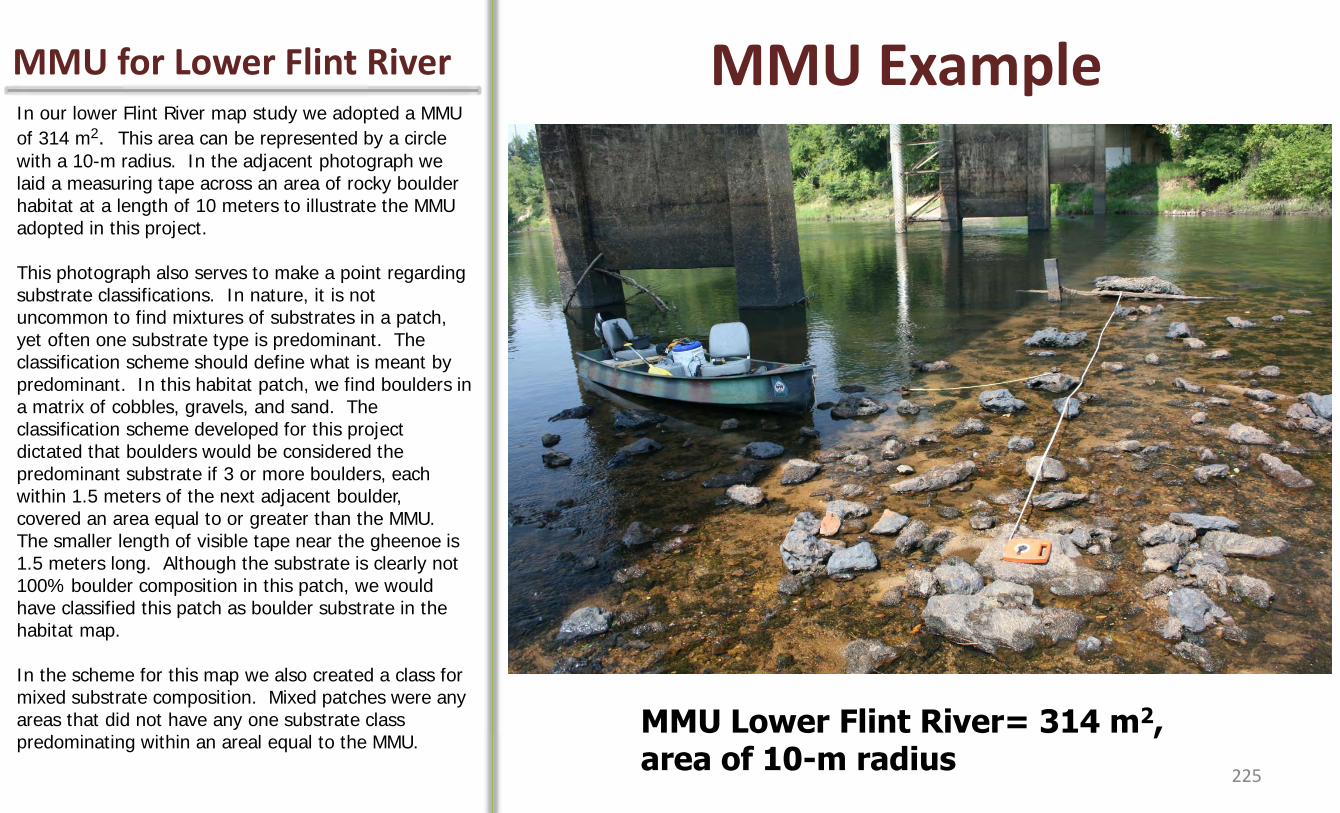
MMU for Lower Flint River MMU Example

MMU Lower Flint River= 314 m2, area of 10-m radius

In our lower Flint River map study we adopted a MMU

of 314 m2. This area can be represented by a circle

with a 10-m radius. In the adjacent photograph we laid a measuring tape across an area of rocky boulder habitat at a length of 10 meters to illustrate the MMU adopted in this project. This photograph also serves to make a point regarding substrate classifications. In nature, it is not uncommon to find mixtures of substrates in a patch, yet often one substrate type is predominant. The classification scheme should define what is meant by predominant. In this habitat patch, we find boulders in a matrix of cobbles, gravels, and sand. The classification scheme developed for this project dictated that boulders would be considered the predominant substrate if 3 or more boulders, each within 1.5 meters of the next adjacent boulder, covered an area equal to or greater than the MMU. The smaller length of visible tape near the gheenoe is 1.5 meters long. Although the substrate is clearly not 100% boulder composition in this patch, we would have classified this patch as boulder substrate in the habitat map. In the scheme for this map we also created a class for mixed substrate composition. Mixed patches were any areas that did not have any one substrate class predominating within an areal equal to the MMU.

225

Inspecting polygon area Checking the MMU

LFR MMU-

314 m2

When a draft of the substrate map is complete, it is possible to inspect and edit the map for adherence to the specified MMU. In the example provided here, there are a two polygons that did not meet the MMU; a red polygon representing an area beyond sonar range (i.e., no sonar data) that is 202 m2 and a yellow polygon representing a sandy patch 274 m2. We could either decompose the sand polygon into the surrounding mixed rocky class (olive color) or adjust the MMU downward for compliance. It would be less appropriate, however, to decompose the 202 m2 polygon into either the pink or grey substrate classes, as these represent areas of uncertainty that were within sonar range during the survey. To preserve the integrity of the accounting system built into this particular classification scheme we would have preserved the 202 m2 polygon in the final map.

226

Common substrates Classes Identified for Mapping Let’s turn our attention to some of the common substrate classes that appear in streams of our work region. Sand patches often exhibit ripple and dune patterning. These textures produce clearly recognizable sonar signatures when scanned. As this photograph illustrates, sand can also exist in plane bed form. Whether sand patches are rippled, dune-like, or plane bed is related to stream velocity and other forces acting on the stream bed.

Sandy (S) 227

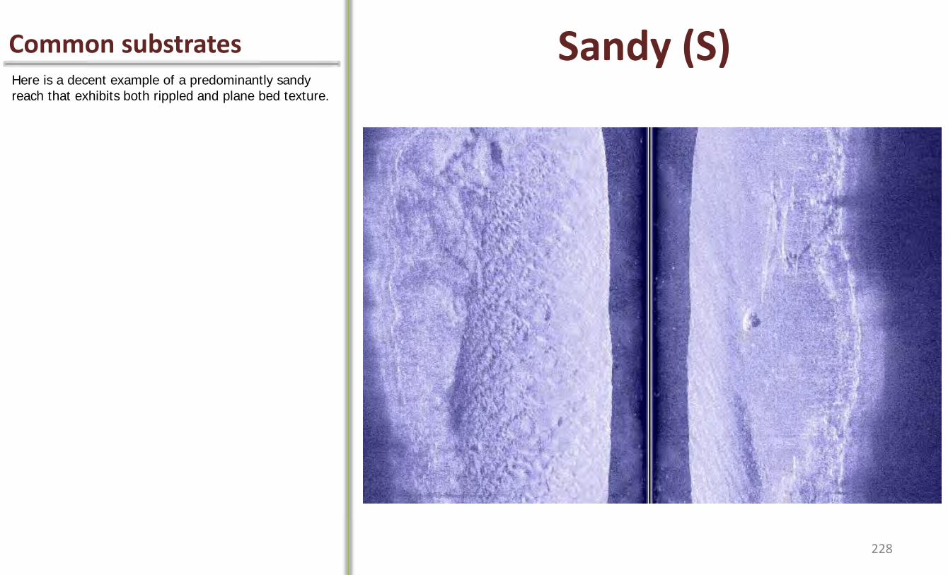
Common substrates Sandy (S) Here is a decent example of a predominantly sandy reach that exhibits both rippled and plane bed texture.

228

Coarse substrates Rocky fine (Rf) Rocky boulder (Rb) It is not uncommon in streams of Southwest Georgia

to find coarse rocky substrates. In this photograph we find cobble, which we describe as rocky fine in our classification scheme, and boulder, called rocky boulder in the scheme. It’s easy to visualize a line that defines the edge separating boulder from cobble substrate in this patch.


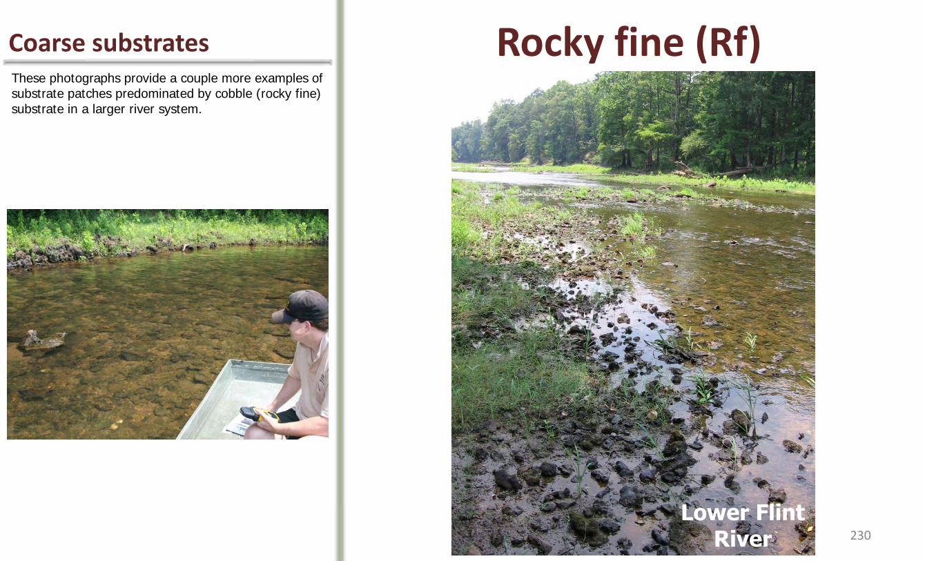
Coarse substrates Rocky fine (Rf) These photographs provide a couple more examples of substrate patches predominated by cobble (rocky fine) substrate in a larger river system.

Lower Flint River 230

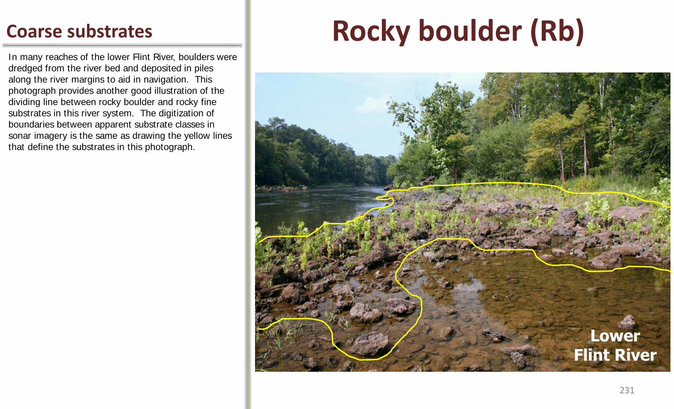
Coarse substrates Rocky boulder (Rb)

Lower Flint River

In many reaches of the lower Flint River, boulders were dredged from the river bed and deposited in piles along the river margins to aid in navigation. This photograph provides another good illustration of the dividing line between rocky boulder and rocky fine substrates in this river system. The digitization of boundaries between apparent substrate classes in sonar imagery is the same as drawing the yellow lines that define the substrates in this photograph.

231

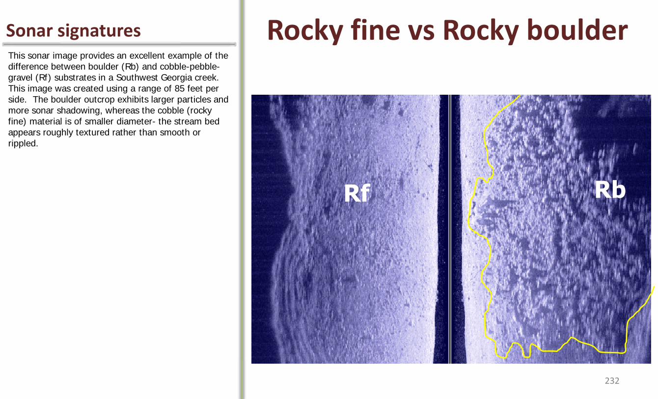
Sonar signatures Rocky fine vs Rocky boulder This sonar image provides an excellent example of the difference between boulder (Rb) and cobble-pebble-gravel (Rf) substrates in a Southwest Georgia creek. This image was created using a range of 85 feet per side. The boulder outcrop exhibits larger particles and more sonar shadowing, whereas the cobble (rocky fine) material is of smaller diameter- the stream bed appears roughly textured rather than smooth or rippled.

Rb Rf

232

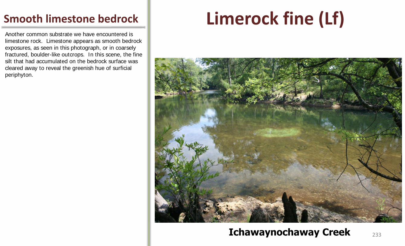
Smooth limestone bedrock Limerock fine (Lf) Another common substrate we have encountered is limestone rock. Limestone appears as smooth bedrock exposures, as seen in this photograph, or in coarsely fractured, boulder-like outcrops. In this scene, the fine silt that had accumulated on the bedrock surface was cleared away to reveal the greenish hue of surficial periphyton.

Ichawaynochaway Creek 233

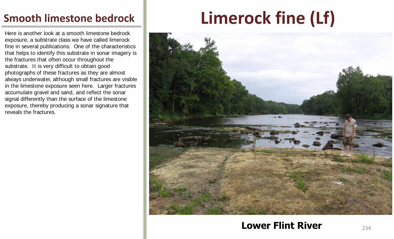
Smooth limestone bedrock Limerock fine (Lf) Here is another look at a smooth limestone bedrock exposure, a substrate class we have called limerock fine in several publications. One of the characteristics that helps to identify this substrate in sonar imagery is the fractures that often occur throughout the substrate. It is very difficult to obtain good photographs of these fractures as they are almost always underwater, although small fractures are visible in the limestone exposure seen here. Larger fractures accumulate gravel and sand, and reflect the sonar signal differently than the surface of the limestone exposure, thereby producing a sonar signature that reveals the fractures.


Smooth limestone bedrock Limerock fine (Lf) This raw image mosaic provides an excellent example of a river reach that is predominantly smooth limestone bedrock. The fractures throughout the limestone are clearly evident here. In our experience, limestone bedrock has a darker tone (color shade) in sonar imagery than sand or rocky fine substrates. And thus, the combination of texture and tone help to discriminate smooth limestone bedrock from other substrate types.

•Sometimes fractured

•Darker tone than sand or rocky fine

235

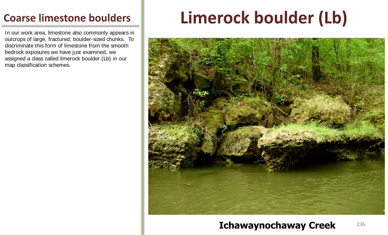
Coarse limestone boulders Limerock boulder (Lb) In our work area, limestone also commonly appears in outcrops of large, fractured, boulder-sized chunks. To discriminate this form of limestone from the smooth bedrock exposures we have just examined, we assigned a class called limerock boulder (Lb) in our map classification schemes.

Ichawaynochaway Creek 236

Coarse limestone boulders Limerock boulder (Lb) In some places the limestone boulders can be massive. Here, boulders are perched atop a limestone wall that drops almost vertically to the riverbed below. At the base of the wall are submerged limestone boulders. This is a great place to find large flathead catfish! The boat ahead is our catfish shocking boat; in my other hand is a net ready to snatch the rolling lunkers.


Accounting for uncertainty Unsure classes (US, UR) It is not uncommon for areas near the margins of the sonar image, or near the banks, to be somewhat distorted. This effect can at least be partly attributed to beam spreading in the far-field, as explained in Session I. Another cause of distortion along the banks can come from the increase in slope as the channel rises to the edge of the bank. Recall that side scan sonar performs best over relatively flat terrains; signal returns coming from a steeply sloped bank will be compressed into a narrow region of image space relative to returns from a flat portion of the channel. Regardless of cause, there are ways to deal with areas of image distortion when preparing a sonar-based habitat map. In past projects we have included a class called “unsure” to represent areas that are difficult to classify due to distortion. It seems prudent to include such a class to account for map uncertainty. In the end, the amount of uncertainty is quantifiable, and uncertain areas are spatially identified. Targeted groundtruthing can be conducted to resolve uncertain areas if deemed necessary.

We have experimented with breaking the unsure class into 2 components- unsure sandy and unsure rocky- by classifying distorted areas as either predominantly sandy or predominantly rocky based on available image information, and contextual information such as whether the area was adjacent to a sandy flat or rocky shoal. This approach has yielded mixed results, see Kaeser and Litts (2010) and Kaeser et al. (2012) for details.

Distorted Areas

238

Accounting for shadowing Sonar Shadow (SS) Areas covered by sonar shadow that cannot be assigned to a substrate class can be digitized and classified as “sonar shadow”. Using a separate class for sonar shadowed areas allows us to quantify this type of data loss. On the other hand, shadowed areas can sometimes be accurately classified using contextual information or other data sources such as air photos. *This annotated sonar image printout is another fine example of the field work undertaken to become familiar with predominant substrates of the region and their sonar signatures.

Sonar shadow

239

Examples of other classes Additional Classes This list represents some of the classes that have appeared in other mapping projects we’ve conducted. This list is by no means comprehensive. We suspect a variety of substrates we haven’t yet seen to exhibit unique and distinguishable sonar signatures. A worthy goal is to evaluate the accuracy of mapping such substrates with low-cost, side scan sonar. We have used the class “No data beyond range” to identify all portions of the wetted stream channel that were beyond the range of the sonar during the survey (thus no image data available). A reliable air photo that shows the wetted channel at flows comparable to those experienced during the survey is necessary to accurately digitize these areas. Likewise, air photos are useful for digitizing the boundaries of mid-channel islands, especially if survey navigation of side channels was not undertaken.

• Mixed rocky

• Bedrock outcrop

• Coarse sand/Gravel

• Clay outcrop, Claystone

• No data beyond range

• Island

• Vegetated Bank 240

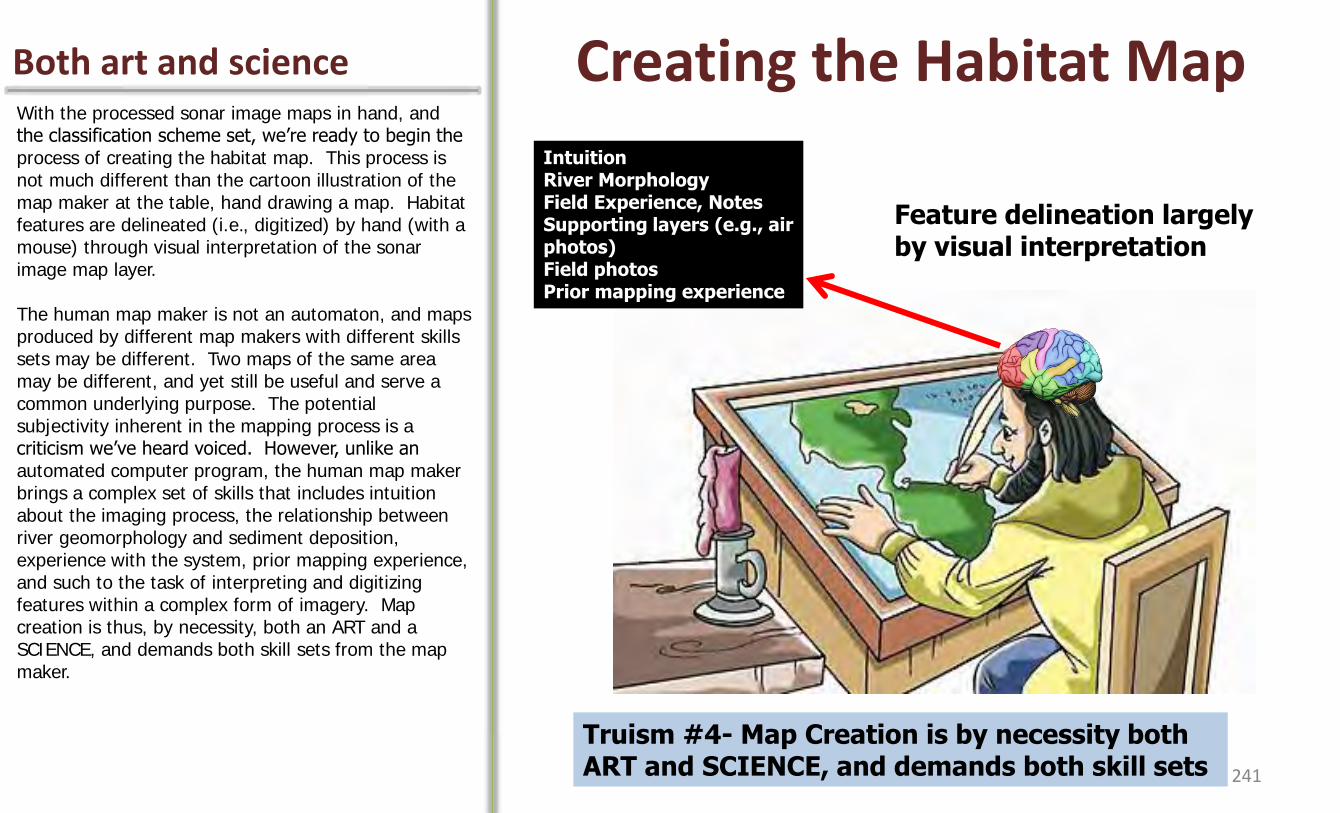
Both art and science Creating the Habitat Map With the processed sonar image maps in hand, and the classification scheme set, we’re ready to begin the process of creating the habitat map. This process is not much different than the cartoon illustration of the map maker at the table, hand drawing a map. Habitat features are delineated (i.e., digitized) by hand (with a mouse) through visual interpretation of the sonar image map layer. The human map maker is not an automaton, and maps produced by different map makers with different skills sets may be different. Two maps of the same area may be different, and yet still be useful and serve a common underlying purpose. The potential subjectivity inherent in the mapping process is a criticism we’ve heard voiced. However, unlike an automated computer program, the human map maker brings a complex set of skills that includes intuition about the imaging process, the relationship between river geomorphology and sediment deposition, experience with the system, prior mapping experience, and such to the task of interpreting and digitizing features within a complex form of imagery. Map creation is thus, by necessity, both an ART and a SCIENCE, and demands both skill sets from the map maker.

Feature delineation largely by visual interpretation

Intuition River Morphology Field Experience, Notes Supporting layers (e.g., air photos) Field photos Prior mapping experience

Truism #4- Map Creation is by necessity both ART and SCIENCE, and demands both skill sets

Feature delineation largely by visual interpretation

241

Can’t my computer do it? Auto-Classification? As sophisticated as computers are these days, it may come as a surprise that automated computer routines for classification of side scan sonar imagery are most likely not (currently) as effective as a trained side scan map maker. We touched on this issue at the beginning of our session on Image Interpretation. The computer obviously doesn’t have the brain of the map maker, or the sense of intuition. What would the computer do upon encountering an image like the one on the right. We know this is woody debris, whose likeness has been distorted through ineffective slant range correction. How would we program the computer to recognize such things? Perhaps someday the computer will be as effective as the human side scan cartographer, but for now we are emboldened by the fact that computers simply can’t do it better than we can.

For additional information- Acoustic Techniques for Seabed Classification (Tech Report 32) by Cooperative Research Centre for Coastal Zone Estuary and Waterway Management http://www.ozcoasts.gov.au/geom_geol/toolkit/Tech_CA_sss.jsp

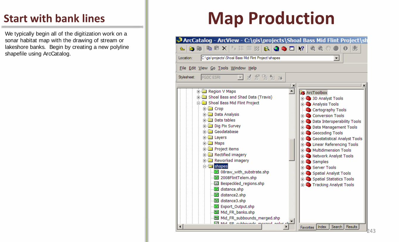
Start with bank lines Map Production We typically begin all of the digitization work on a sonar habitat map with the drawing of stream or lakeshore banks. Begin by creating a new polyline shapefile using ArcCatalog.

243

Enable snapping Stream bank digitization Load the newly created bank line shapefile into the map project and project the file to the appropriate UTM zone. Initiate an editing session on the line, and make sure to enable snapping of ends for the polyline.

Snapping is so important during habitat map production, the topic deserves additional attention. Snapping enables the joining of two adjacent line segments. Joining adjacent line segments will be necessary whenever there is a break in the digitization process when working on bank (or substrate) lines. Without snapping enabled, it is quite possible to create a line segment that appears to be connected to the nearest segment, when in fact a very small gap exists between the segments. This gap may only be visible when zooming in at a very fine scale. Such gaps pose major problems later when line segments are merged, and the enclosed areas converted to a set of polygons. We wish to avoid such unwanted gaps at all costs, and do so by setting up and enabling the snapping options properly. Please consult the ArcGIS Help menu to learn more about snapping. In ArcGIS 10 the form of snapping of interest is called “classic snapping”. This option must be enabled under the General Editing Options. Also consult the help menu to learn about “snap tips”, and “sticky move” and “snapping tolerances”.

With snapping enabled, we begin digitizing bank lines by zooming in to imagery at the appropriate scale and point-and-clicking our way along the bank margin to draw the line.

• Load shapefile

• Initiate an editing session, enable snapping

• Zoom to appropriate scale and begin digitizing 244

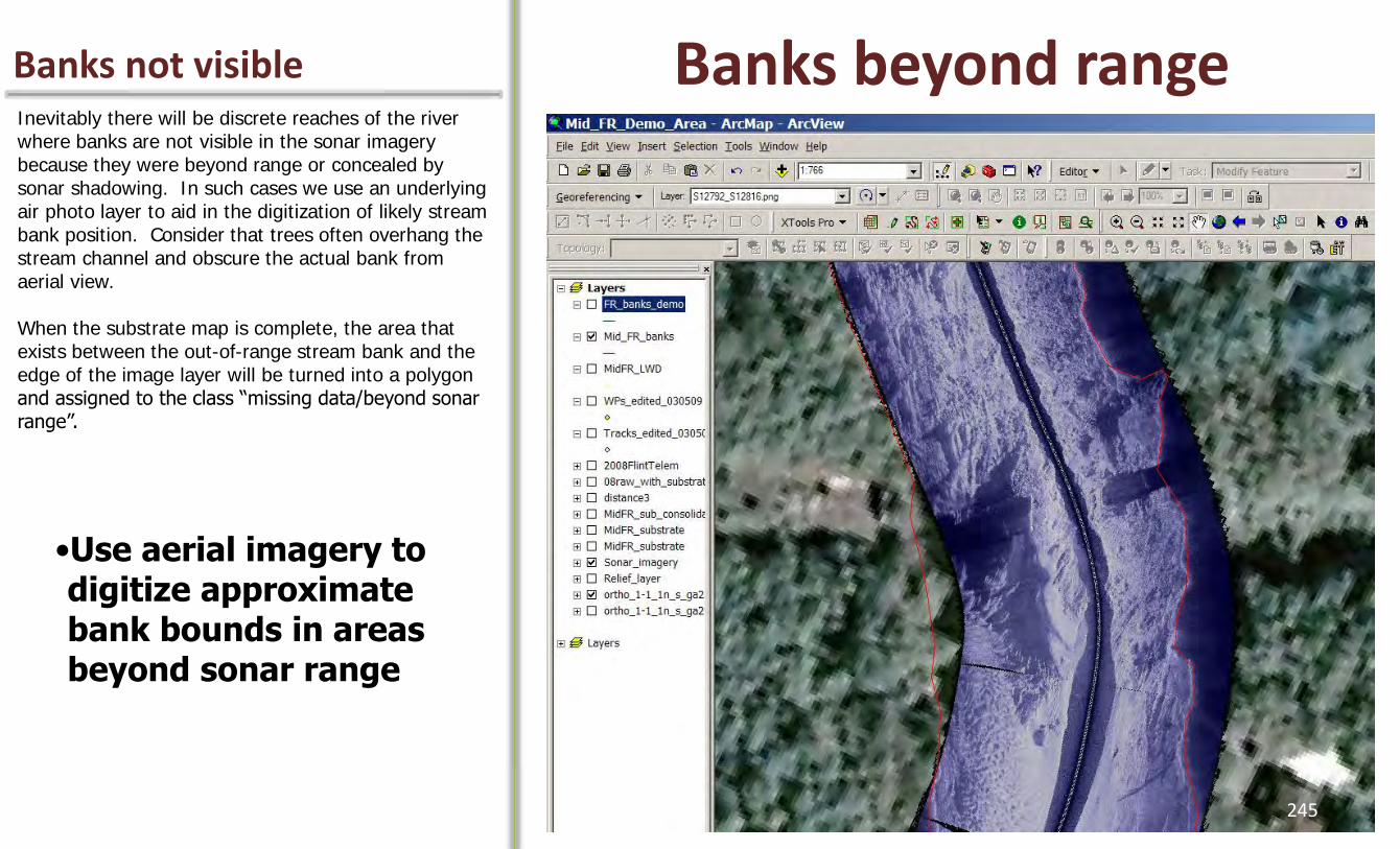
Banks not visible Banks beyond range Inevitably there will be discrete reaches of the river where banks are not visible in the sonar imagery because they were beyond range or concealed by sonar shadowing. In such cases we use an underlying air photo layer to aid in the digitization of likely stream bank position. Consider that trees often overhang the stream channel and obscure the actual bank from aerial view. When the substrate map is complete, the area that exists between the out-of-range stream bank and the edge of the image layer will be turned into a polygon and assigned to the class “missing data/beyond sonar range”.

•Use aerial imagery to digitize approximate bank bounds in areas beyond sonar range

245

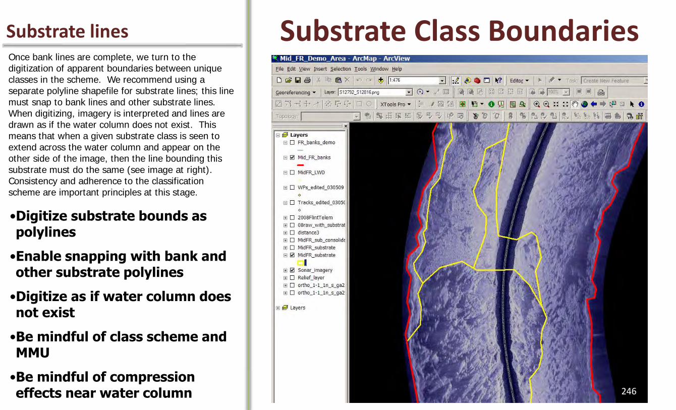
Substrate lines Substrate Class Boundaries Once bank lines are complete, we turn to the digitization of apparent boundaries between unique classes in the scheme. We recommend using a separate polyline shapefile for substrate lines; this line must snap to bank lines and other substrate lines. When digitizing, imagery is interpreted and lines are drawn as if the water column does not exist. This means that when a given substrate class is seen to extend across the water column and appear on the other side of the image, then the line bounding this substrate must do the same (see image at right). Consistency and adherence to the classification scheme are important principles at this stage.

•Digitize substrate bounds as polylines

•Enable snapping with bank and other substrate polylines

•Digitize as if water column does not exist

•Be mindful of class scheme and MMU

•Be mindful of compression effects near water column 246

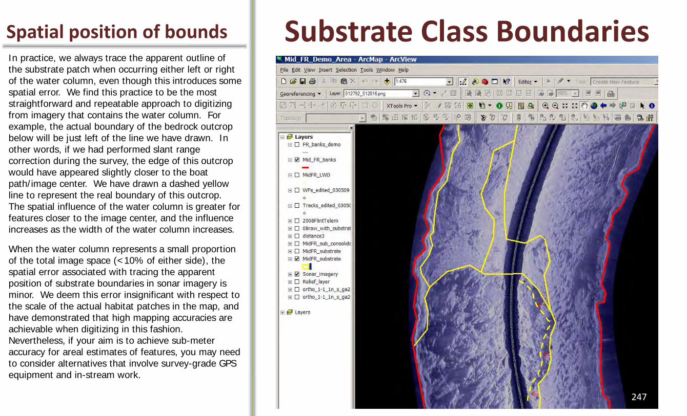
Spatial position of bounds Substrate Class Boundaries In practice, we always trace the apparent outline of the substrate patch when occurring either left or right of the water column, even though this introduces some spatial error. We find this practice to be the most straightforward and repeatable approach to digitizing from imagery that contains the water column. For example, the actual boundary of the bedrock outcrop below will be just left of the line we have drawn. In other words, if we had performed slant range correction during the survey, the edge of this outcrop would have appeared slightly closer to the boat path/image center. We have drawn a dashed yellow line to represent the real boundary of this outcrop. The spatial influence of the water column is greater for features closer to the image center, and the influence increases as the width of the water column increases.

When the water column represents a small proportion of the total image space (<10% of either side), the spatial error associated with tracing the apparent position of substrate boundaries in sonar imagery is minor. We deem this error insignificant with respect to the scale of the actual habitat patches in the map, and have demonstrated that high mapping accuracies are achievable when digitizing in this fashion. Nevertheless, if your aim is to achieve sub-meter accuracy for areal estimates of features, you may need to consider alternatives that involve survey-grade GPS equipment and in-stream work.

247

Raw images as reference Using raw images One of the benefits of the snapshot approach is the ability to easily reference the raw sonar image data set during the mapping process. The process of image rectification can sometimes slightly degrade image quality- after all, pixels are being rearranged to fit the image to its real-world shape. It’s helpful to be able to quickly reference and retrieve the original raw image when confronted with a difficult-to-interpret area. The raw image sometimes helps to clarify the interpretation.

Raw images are referenced during the mapping process by overlaying the waypoint data set on the sonar image map layer. Each waypoint contains the raw image ID number that can be used to retrieve the image from the appropriate folder on an adjacent computer screen. Don’t have dual screens? Well, if you plan to do much sonar habitat mapping, we highly recommend the dual screen set-up. The higher quality screen can be used to display the sonar imagery, and the other screen can be used to display your computer directory, ArcCatalog, Excel tables, or any other programs in use during the mapping process.

In the example provided on the right, we are showing the use of the raw image to interpret what was going on in an area where an image failed to rectify due to the boat turn. These issues can now largely be resolved using an approach Thom developed to correct warping and rectification failures (another benefit of the snapshot approach!). 248

A substrate layer unfolds Create and Classify Polygons Once all substrate bounds are complete, the substrate lines shapefile is merged with the bank lines shapefile. Using the Data Management Tools “Feature to Polygon” option under the Features tab (enabled at the ArcINFO level) all areas bound by polylines can be converted to polygons. We advise the creation of a geodatabase for the project that contains a domain with all substrate classes in the map classification scheme. The polygon shapefile can be loaded into this geodatabase and assigned the domain. When editing the polygon file, each polygon is selected and the proper substrate class is easily assigned via selection from a drop-down menu displayed in the attribute table of the polygon file. Each class can be symbolized with a unique color; as the classification process unfolds the map becomes a rich mosaic of patches.

•Merge substrate and bank polylines, convert areas bound by lines to polygons

•Create geodatabase with domain that includes all substrate classes- load polygon file

•Assign class to each polygon

•Examine map at several scales to assist with interpretation

249

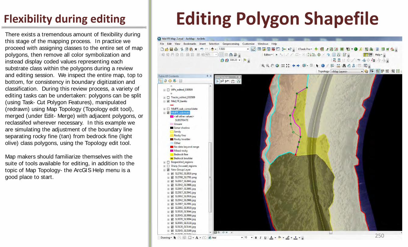
Flexibility during editing Editing Polygon Shapefile There exists a tremendous amount of flexibility during this stage of the mapping process. In practice we proceed with assigning classes to the entire set of map polygons, then remove all color symbolization and instead display coded values representing each substrate class within the polygons during a review and editing session. We inspect the entire map, top to bottom, for consistency in boundary digitization and classification. During this review process, a variety of editing tasks can be undertaken: polygons can be split (using Task- Cut Polygon Features), manipulated (redrawn) using Map Topology (Topology edit tool), merged (under Edit- Merge) with adjacent polygons, or reclassifed wherever necessary. In this example we are simulating the adjustment of the boundary line separating rocky fine (tan) from bedrock fine (light olive) class polygons, using the Topology edit tool. Map makers should familiarize themselves with the suite of tools available for editing, in addition to the topic of Map Topology- the ArcGIS Help menu is a good place to start.

250

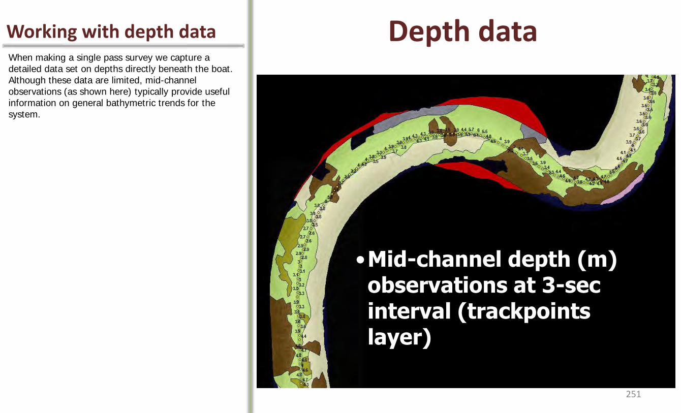
Working with depth data Depth data When making a single pass survey we capture a detailed data set on depths directly beneath the boat. Although these data are limited, mid-channel observations (as shown here) typically provide useful information on general bathymetric trends for the system.

•Mid-channel depth (m) observations at 3-sec interval (trackpoints layer)

251

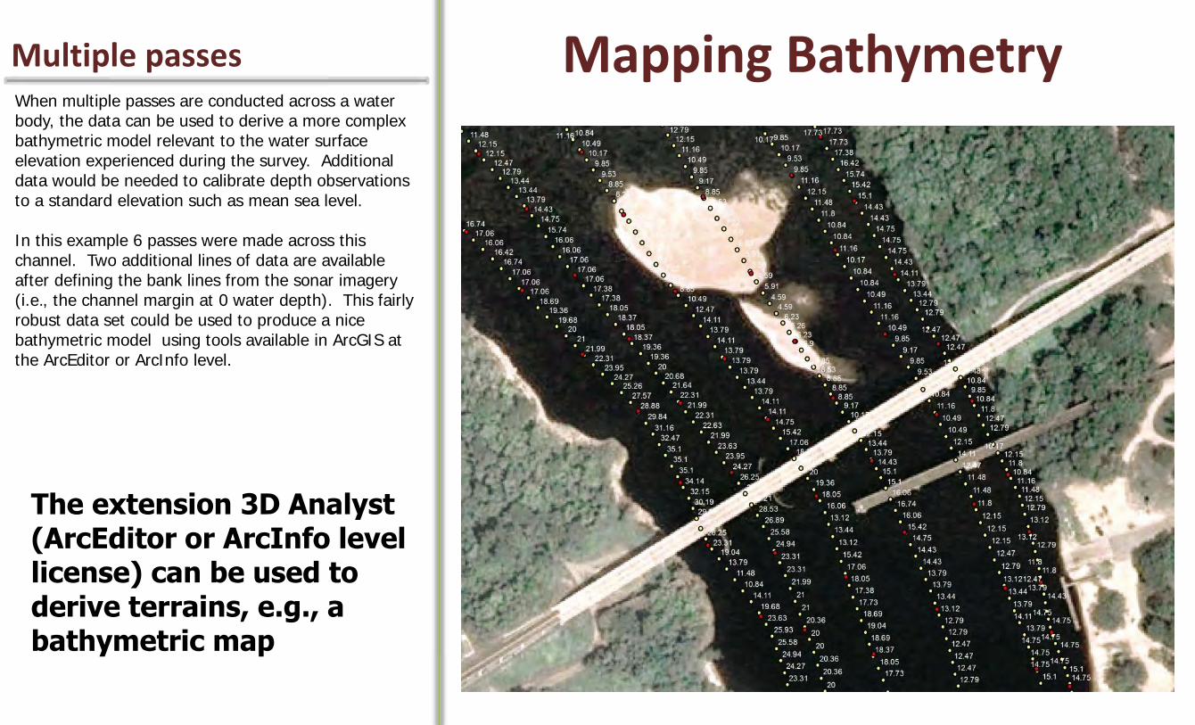
Multiple passes Mapping Bathymetry When multiple passes are conducted across a water body, the data can be used to derive a more complex bathymetric model relevant to the water surface elevation experienced during the survey. Additional data would be needed to calibrate depth observations to a standard elevation such as mean sea level. In this example 6 passes were made across this channel. Two additional lines of data are available after defining the bank lines from the sonar imagery (i.e., the channel margin at 0 water depth). This fairly robust data set could be used to produce a nice bathymetric model using tools available in ArcGIS at the ArcEditor or ArcInfo level.

The extension 3D Analyst (ArcEditor or ArcInfo level license) can be used to derive terrains, e.g., a bathymetric map

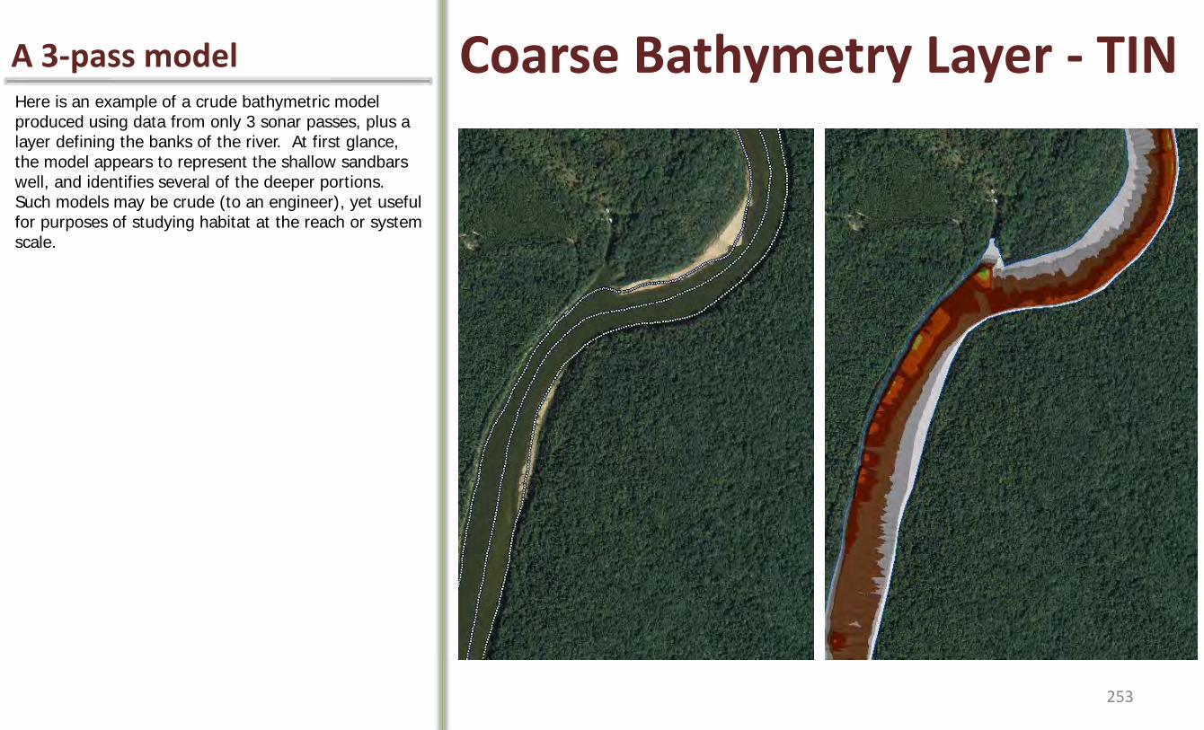
A 3-pass model Coarse Bathymetry Layer - TIN Here is an example of a crude bathymetric model produced using data from only 3 sonar passes, plus a layer defining the banks of the river. At first glance, the model appears to represent the shallow sandbars well, and identifies several of the deeper portions. Such models may be crude (to an engineer), yet useful for purposes of studying habitat at the reach or system scale.

253

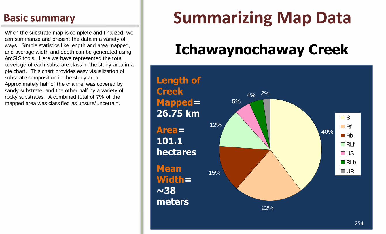
Basic summary Summarizing Map Data When the substrate map is complete and finalized, we can summarize and present the data in a variety of ways. Simple statistics like length and area mapped, and average width and depth can be generated using ArcGIS tools. Here we have represented the total coverage of each substrate class in the study area in a pie chart. This chart provides easy visualization of substrate composition in the study area. Approximately half of the channel was covered by sandy substrate, and the other half by a variety of rocky substrates. A combined total of 7% of the mapped area was classified as unsure/uncertain.


Length of Creek Mapped= 26.75 km

Area= 101.1 hectares

Mean Width= ~38 meters

40%

22%

15%

12%

5%4% 2%

S

Rf

Rb

RLf

US

RLb

UR

254

Longitudinal trends Summarizing Map Data A slightly more sophisticated approach to summarizing map data that reveals longitudinal trends involves extracting data from fixed reaches. In this example we created a polygon shapefile that overlaid the river channel and subset the polygon into 1-km blocks. (Although difficult to see in the image on the right, the outline of this polygon file is displayed in yellow in panel 2). This shapefile was used to clip and summarize data within each 1-km reach of the river map.

Another approach

•Divide river into reaches (eg. 1km)

•Extract and summarize data by reach

255

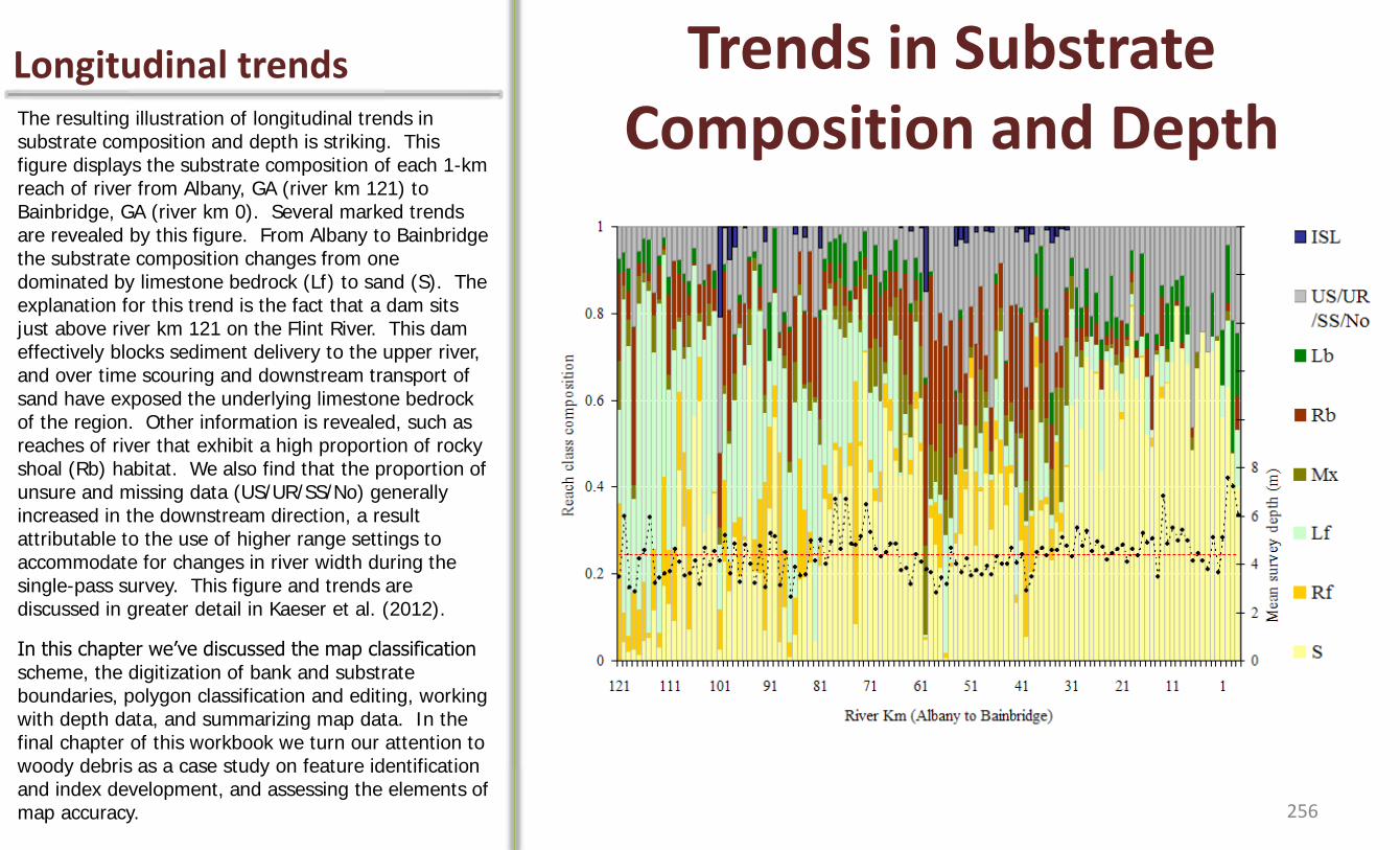
Longitudinal trends Trends in Substrate Composition and Depth The resulting illustration of longitudinal trends in

substrate composition and depth is striking. This figure displays the substrate composition of each 1-km reach of river from Albany, GA (river km 121) to Bainbridge, GA (river km 0). Several marked trends are revealed by this figure. From Albany to Bainbridge the substrate composition changes from one dominated by limestone bedrock (Lf) to sand (S). The explanation for this trend is the fact that a dam sits just above river km 121 on the Flint River. This dam effectively blocks sediment delivery to the upper river, and over time scouring and downstream transport of sand have exposed the underlying limestone bedrock of the region. Other information is revealed, such as reaches of river that exhibit a high proportion of rocky shoal (Rb) habitat. We also find that the proportion of unsure and missing data (US/UR/SS/No) generally increased in the downstream direction, a result attributable to the use of higher range settings to accommodate for changes in river width during the single-pass survey. This figure and trends are discussed in greater detail in Kaeser et al. (2012).

In this chapter we’ve discussed the map classification scheme, the digitization of bank and substrate boundaries, polygon classification and editing, working with depth data, and summarizing map data. In the final chapter of this workbook we turn our attention to woody debris as a case study on feature identification and index development, and assessing the elements of map accuracy. 256

Session IV- Part B Mapping Large Woody Debris Let’s turn our attention to the topic of mapping large woody debris with side scan sonar. Our earliest endeavors with the Humminbird SI system involved this element of habitat. Given the importance of wood to the ecology of streams of the Southeast Coastal Plain, we set out to determine if side scan sonar could be used to reliably quantify and map large woody debris in the turbid, nonwadeble streams of the region. The timing couldn’t have been better for us in that 2007 proved to be year of epic drought that led to low and clear water conditions in our study streams. Much of the groundtruth work was conducted by swimming, snorkeling, and diving- the perfect prescription for field work during a South Georgia summer. Large woody debris has been variously defined in the literature; we used a common definition that specifies large woody debris (LWD) as any piece of wood that is greater than, or equal to 10 cm in diameter over a length of 1.5 meters or more. I asked Josh, our habitat intern, to find a piece of wood that just qualified as LWD. The log he is holding is exactly 10 cm diameter, and is about 2 meters long (the red line represents 1.5 meters). When we talk of mapping LWD we are talking about pieces of wood this size or larger.

a piece of wood >10cm diameter & > 1.5 m long

257

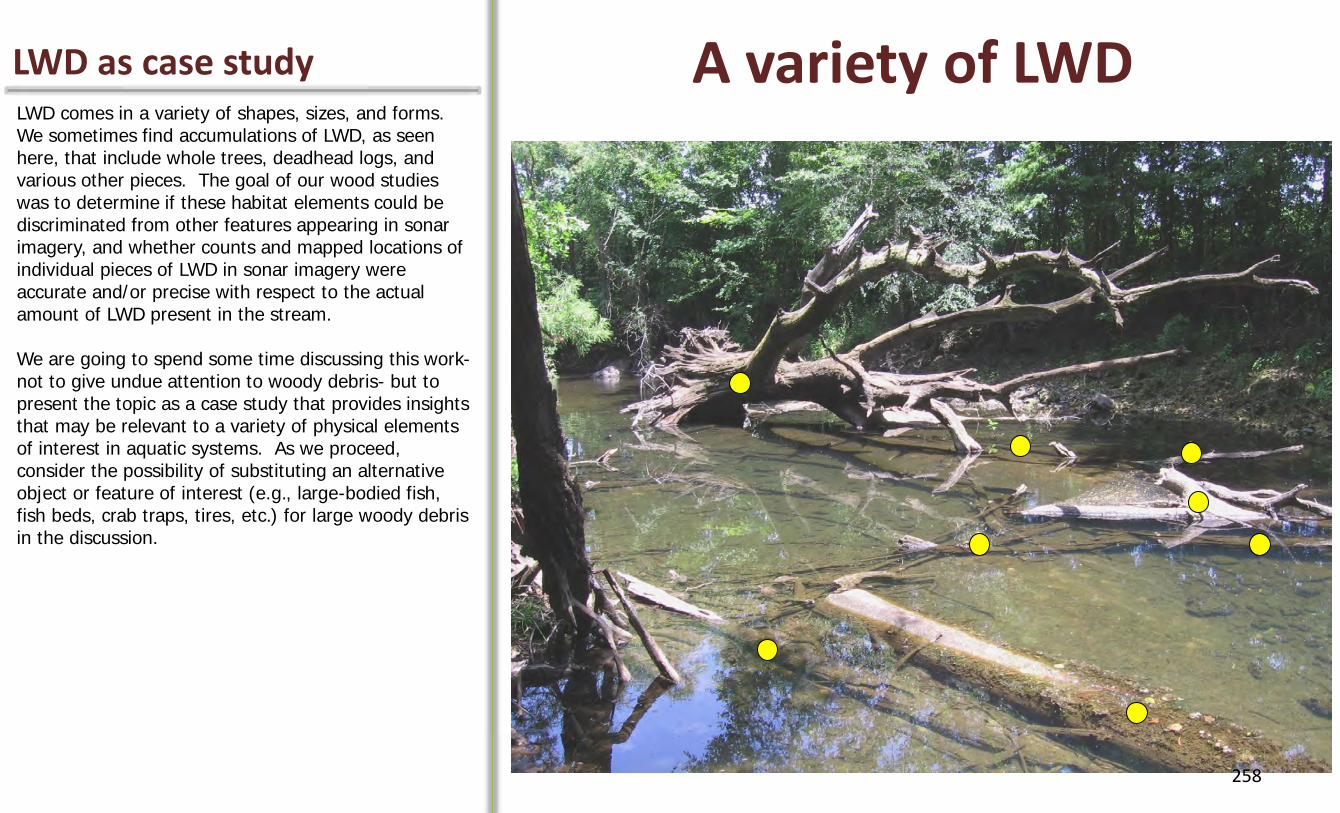
LWD as case study A variety of LWD LWD comes in a variety of shapes, sizes, and forms. We sometimes find accumulations of LWD, as seen here, that include whole trees, deadhead logs, and various other pieces. The goal of our wood studies was to determine if these habitat elements could be discriminated from other features appearing in sonar imagery, and whether counts and mapped locations of individual pieces of LWD in sonar imagery were accurate and/or precise with respect to the actual amount of LWD present in the stream. We are going to spend some time discussing this work- not to give undue attention to woody debris- but to present the topic as a case study that provides insights that may be relevant to a variety of physical elements of interest in aquatic systems. As we proceed, consider the possibility of substituting an alternative object or feature of interest (e.g., large-bodied fish, fish beds, crab traps, tires, etc.) for large woody debris in the discussion.

258

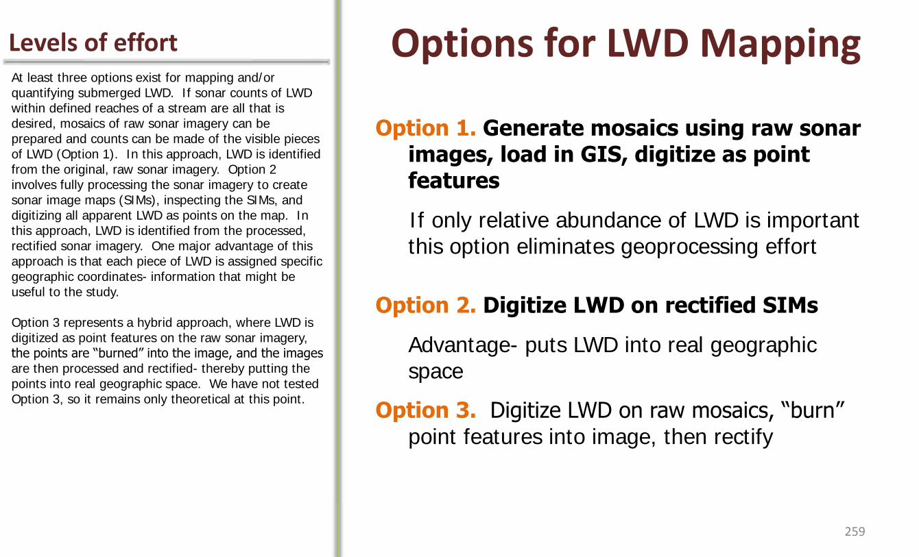
Levels of effort Options for LWD Mapping At least three options exist for mapping and/or quantifying submerged LWD. If sonar counts of LWD within defined reaches of a stream are all that is desired, mosaics of raw sonar imagery can be prepared and counts can be made of the visible pieces of LWD (Option 1). In this approach, LWD is identified from the original, raw sonar imagery. Option 2 involves fully processing the sonar imagery to create sonar image maps (SIMs), inspecting the SIMs, and digitizing all apparent LWD as points on the map. In this approach, LWD is identified from the processed, rectified sonar imagery. One major advantage of this approach is that each piece of LWD is assigned specific geographic coordinates- information that might be useful to the study. Option 3 represents a hybrid approach, where LWD is digitized as point features on the raw sonar imagery, the points are “burned” into the image, and the images are then processed and rectified- thereby putting the points into real geographic space. We have not tested Option 3, so it remains only theoretical at this point.

Option 1. Generate mosaics using raw sonar images, load in GIS, digitize as point features

If only relative abundance of LWD is important this option eliminates geoprocessing effort

Option 2. Digitize LWD on rectified SIMs

Advantage- puts LWD into real geographic space

Option 3. Digitize LWD on raw mosaics, “burn” point features into image, then rectify

259

Option 1 details Option 1. Digitize LWD in Raw Image Mosaics

(using Irfanview and ArcGIS)

Following Option 1 we batch crop the raw sonar images from the study area, then use the image matching tool in Thom’s Sonar Toolkit to clip images at overlap points. The Create Panorama Image function in IrfanView is then used to prepare large, seamless mosaics of the clipped, raw (unrectified) imagery. The mosaics are loaded and viewed in ArcGIS (or viewed in any other image viewing program) to derive counts of apparent LWD.

1) Batch crop raw images using Irfanview (crop settings file provided)

2) Use Image Matching Tool to clip images at overlap point

3) Use Irfanview to generate mosaics from clipped images

260

Consider this cache Here is a nice cache of deadhead logs, exposed during the extreme drought conditions of 2007 in Southwest Georgia.

Chickasawhatchee Creek Log Cache

261

Counts from raw mosaic This is the corresponding raw image mosaic prepared for the Chickasawhatchee Creek log cache. The yellow arrow identifies the location from which the photograph was taken for purposes of referencing individual logs seen in the sonar imagery to the logs in the cache photograph. This mosaic, when loaded in ArcGIS as a raster file, can be inspected to assign points to each piece of LWD as shown here. When done, a polygon can be created to bound the study area and used as a feature to clip and tally the number of pieces of LWD.

Option 1 for LWD Mapping

•Load reach mosaic in GIS

•Create point shapefile for reach

•Digitize LWD identified in reach mosaic

262

Counts from SIMs Option 2 for LWD mapping is similar in approach, except that the imagery is rectified, and the sonar image map layers are used to identify and map actual locations of the LWD. In this example we used a point shapefile symbolized as a yellow X to identify pieces of LWD.

Option 2 for LWD Mapping

•Create point shapefile for LWD

•Digitize LWD identified in SIMs

•Can extract LWD counts by clipping features from portions of the map and summarizing

263

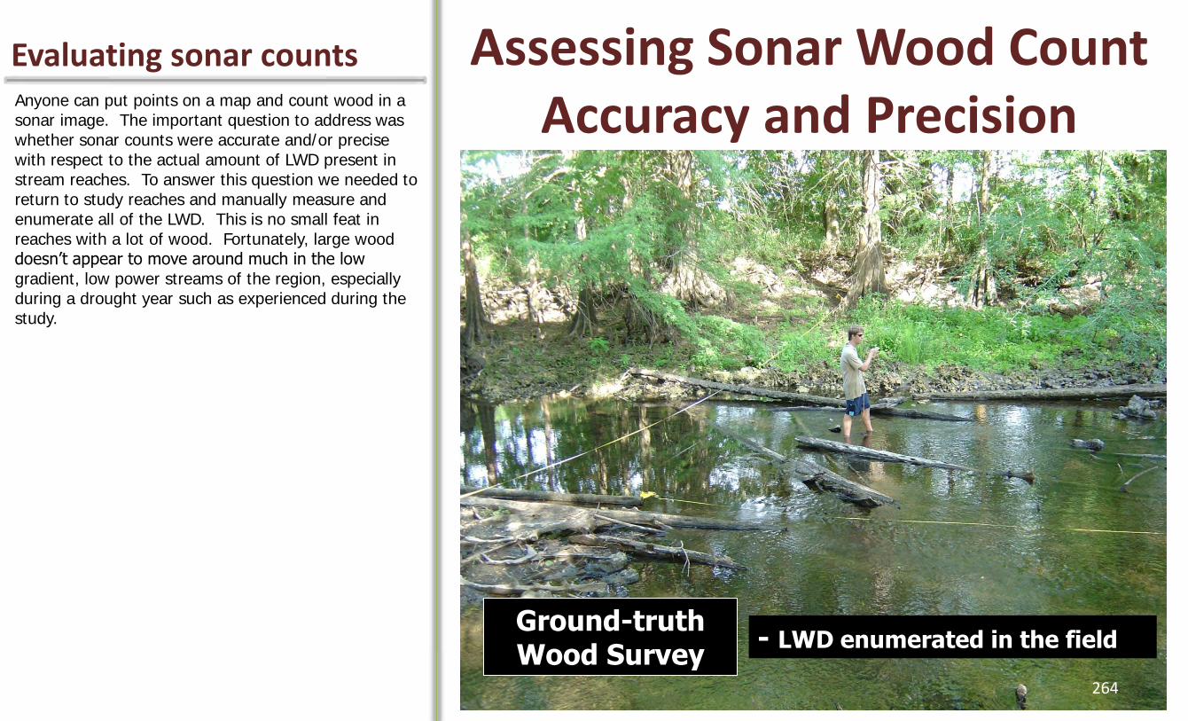
Evaluating sonar counts Anyone can put points on a map and count wood in a sonar image. The important question to address was whether sonar counts were accurate and/or precise with respect to the actual amount of LWD present in stream reaches. To answer this question we needed to return to study reaches and manually measure and enumerate all of the LWD. This is no small feat in reaches with a lot of wood. Fortunately, large wood doesn’t appear to move around much in the low gradient, low power streams of the region, especially during a drought year such as experienced during the study.

Assessing Sonar Wood Count Accuracy and Precision

Ground-truth Wood Survey

- LWD enumerated in the field

264

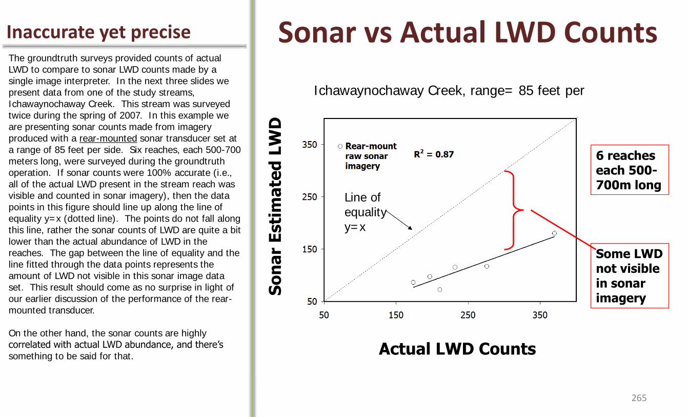
Inaccurate yet precise The groundtruth surveys provided counts of actual LWD to compare to sonar LWD counts made by a single image interpreter. In the next three slides we present data from one of the study streams, Ichawaynochaway Creek. This stream was surveyed twice during the spring of 2007. In this example we are presenting sonar counts made from imagery produced with a rear-mounted sonar transducer set at a range of 85 feet per side. Six reaches, each 500-700 meters long, were surveyed during the groundtruth operation. If sonar counts were 100% accurate (i.e., all of the actual LWD present in the stream reach was visible and counted in sonar imagery), then the data points in this figure should line up along the line of equality y=x (dotted line). The points do not fall along this line, rather the sonar counts of LWD are quite a bit lower than the actual abundance of LWD in the reaches. The gap between the line of equality and the line fitted through the data points represents the amount of LWD not visible in this sonar image data set. This result should come as no surprise in light of our earlier discussion of the performance of the rear-mounted transducer. On the other hand, the sonar counts are highly correlated with actual LWD abundance, and there’s something to be said for that.

Sonar vs Actual LWD Counts

Actual LWD Counts

So

na

r E

sti

ma

ted

LW

D

6 reaches each 500-700m long

Some LWD not visible in sonar imagery

Line of equality y=x

Ichawaynochaway Creek, range= 85 feet per

265

Effects of transducer In this figure we have added the sonar count data generated from imagery created with a front-mounted transducer. Counts made from front-mounted imagery were more accurate- more of the LWD present in the stream reach was visible. This result is consistent with our observations of enhanced image quality when using a front-mounted transducer. Sonar counts still fall below the line of equality, thus we still cannot identify all of the LWD in sonar imagery that was actually present in the study reaches. Nonetheless, the correlation between sonar counts made with the front-mount transducer and actual LWD is high and identical to that of the rear-mount transducer. High correlation values indicate that sonar counts are precise. In addition to the consistent performance of the Humminbird system, we attribute high precision of sonar counts to the ability of the sonar interpreter to maintain consistency throughout the review process. With high precision, the sonar count data set could be used to provide a reliable index of relative abundance of LWD in the reaches. Alternatively, linear regression could be used to calibrate sonar counts to actual abundance of LWD in reaches that were not groundtruthed.


Actual LWD Counts

So

na

r E

sti

ma

ted

LW

D

Ichawaynochaway Creek, range= 85 feet per side

• Front-mount reveals more LWD

• Sonar counts are precise- provide index to LWD

• Linear regression to calibrate sonar counts to actual LWD

266

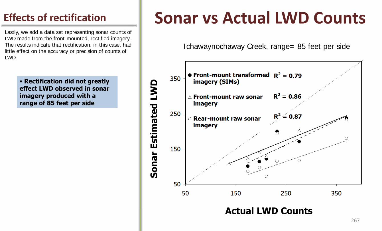
Effects of rectification Lastly, we add a data set representing sonar counts of LWD made from the front-mounted, rectified imagery. The results indicate that rectification, in this case, had little effect on the accuracy or precision of counts of LWD.


• Rectification did not greatly effect LWD observed in sonar imagery produced with a range of 85 feet per side

Actual LWD Counts

So

na

r E

sti

ma

ted

LW

D

Ichawaynochaway Creek, range= 85 feet per side

267

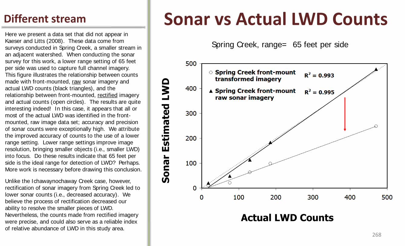
Different stream Here we present a data set that did not appear in Kaeser and Litts (2008). These data come from surveys conducted in Spring Creek, a smaller stream in an adjacent watershed. When conducting the sonar survey for this work, a lower range setting of 65 feet per side was used to capture full channel imagery. This figure illustrates the relationship between counts made with front-mounted, raw sonar imagery and actual LWD counts (black triangles), and the relationship between front-mounted, rectified imagery and actual counts (open circles). The results are quite interesting indeed! In this case, it appears that all or most of the actual LWD was identified in the front-mounted, raw image data set; accuracy and precision of sonar counts were exceptionally high. We attribute the improved accuracy of counts to the use of a lower range setting. Lower range settings improve image resolution, bringing smaller objects (i.e., smaller LWD) into focus. Do these results indicate that 65 feet per side is the ideal range for detection of LWD? Perhaps. More work is necessary before drawing this conclusion.

Unlike the Ichawaynochaway Creek case, however, rectification of sonar imagery from Spring Creek led to lower sonar counts (i.e., decreased accuracy). We believe the process of rectification decreased our ability to resolve the smaller pieces of LWD. Nevertheless, the counts made from rectified imagery were precise, and could also serve as a reliable index of relative abundance of LWD in this study area.


Actual LWD Counts

So

na

r E

sti

ma

ted

LW

D

Spring Creek, range= 65 feet per side

268

Food for thought During our studies of wood we began learning about the performance of the system and the work required to develop and evaluate sonar habitat mapping applications. We learned, through first-hand experience, that some objects simply imaged better than others due to a variety of factors such as orientation, position in the stream channel, size, and density. We learned that the sonar range setting affected our ability to resolve objects. Image processing also had the potential to affect object resolution, yet the effects were variable and appeared to be influenced by factors such as range and the general size of the objects. These lessons provide a lot of food for thought when working to develop and evaluate side scan sonar mapping applications. What ranges should be used when targeting an object- should imagery be rectified or is the raw format best?

Lessons Learned

• Some objects image better than others due to orientation, context, size, and density

• As range decreases, more LWD (smaller pieces/objects) can be discerned

• Rectification can affect object definition and recognition, but the effects appear variable (driven by other factors, like range used)

269

Our work with wood and low-cost, side scan sonar is featured in a 2008 Fisheries article. This article contains additional recommendations, such as the use of non-randomly selected reaches during the development of a system-specific index of woody debris abundance. The intent of this article was two-fold- to draw attention to a resource that is imperiled and understudied, yet common to the region (i.e., deadhead logs), and to introduce the concept of assessing wood at the landscape scale using a low-cost, remote sensing tool. We would be pleased if this case study helps to stimulate additional work to develop and evaluate applications of low-cost sonar habitat mapping. Let’s step away from woody debris, and revisit the 5- step process of developing a sonar-based habitat map to see how far we have come.

Other Recommendations

E.g., Calibrating Wood Counts

Non-randomly select reaches (eg. 100 m) that represent full range of wood abundance (low to high, from sonar counts) for field counts during low flow conditions

Pursue applications

270

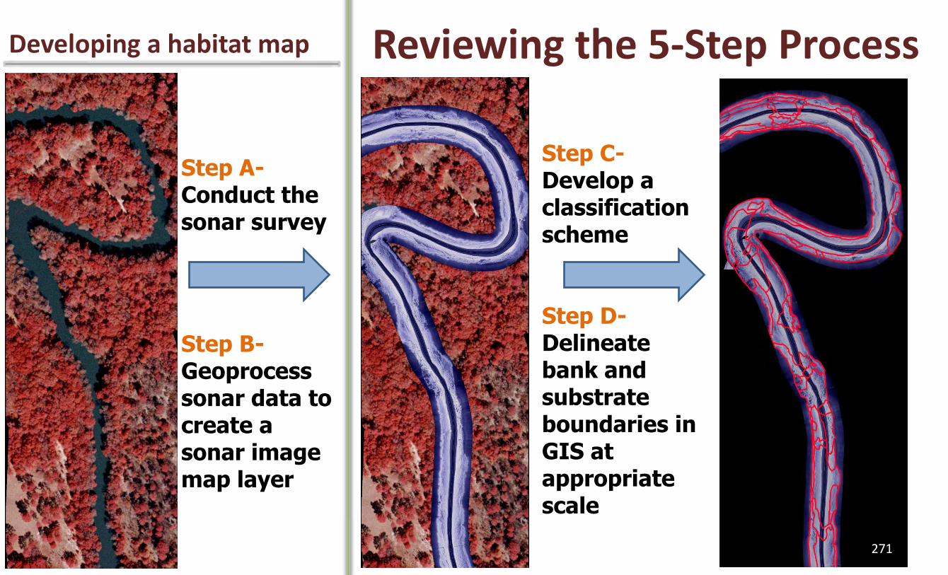
Reviewing the 5-Step Process

Step A- Conduct the sonar survey

Step B- Geoprocess sonar data to create a sonar image map layer

Step C- Develop a classification scheme

Step D- Delineate bank and substrate boundaries in GIS at appropriate scale

Developing a habitat map

271

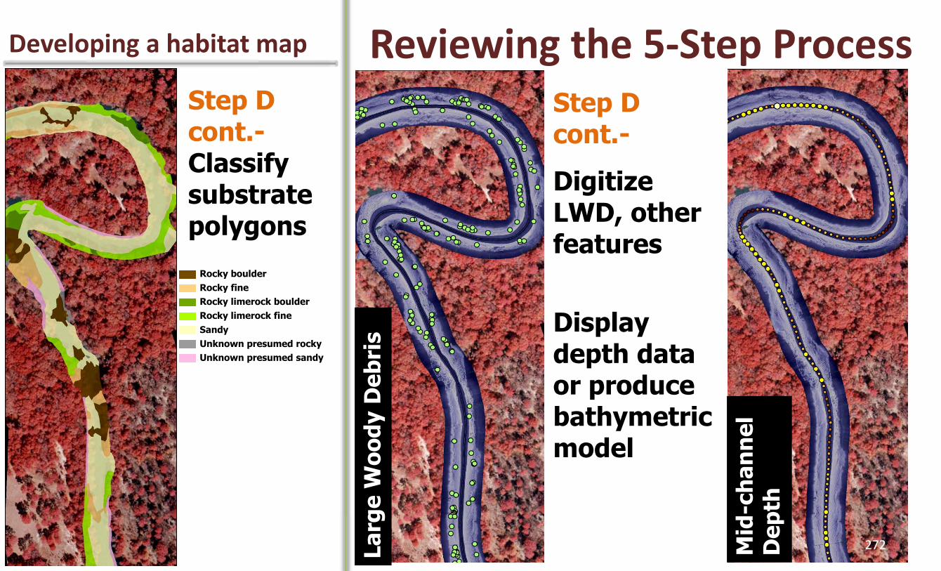
Reviewing the 5-Step Process Developing a habitat map

Step D cont.- Classify substrate polygons

SUBSTRATE

Rocky boulder

Rocky fine

Rocky limerock boulder

Rocky limerock fine

Sandy

Unknown presumed rocky

Unknown presumed sandy

La

rge

Wo

od

y D

eb

ris

Mid

-ch

an

ne

l D

ep

th

Step D cont.-

Digitize LWD, other features

Display depth data or produce bathymetric model

272

A final, yet very important step in the process of developing a habitat map is the assessment of map accuracy. It’s way too easy to assume that your map is correct once it’s staring back at you on the computer screen. Your map- like any model- is merely an abstraction of reality. Like any good statistical or theoretical model, the map (and hence the map maker’s skills) must be put to the test and validated. There are three principle elements of map accuracy that are relevant to sonar-based habitat maps. The first element is dimensional accuracy. Dimensional accuracy relates to the size and shape of features that appear in the rectified sonar image map layers. Is it safe to assume that the sonar image maps are dimensionally correct? The second element is positional accuracy. An assessment of positional accuracy involves determining how much error is associated with locating map features in the field. A map object may be dimensionally correct, yet in the wrong, real-world location. The third element is classification accuracy. An assessment of classification accuracy involves determining whether features in the map were correctly classified. A fantastic reference book on the topic of map accuracy assessment can be found in Gongalton and Green (1999). This book was recommended to help guide our work during this critical step of the mapping process.

Assessing Map Accuracy Step E- Map accuracy

1) Dimensional Accuracy- are

rectified images dimensionally correct?

2) Positional Accuracy- how much

error is associated with locating map features in the field?

3) Classification Accuracy- are

substrate polygons classified correctly?

*Reference- Congalton, R.G., and K. Green. 1999. Assessing the accuracy of remotely sensed data: principles and practices. Lewis Publishers, New York.

273

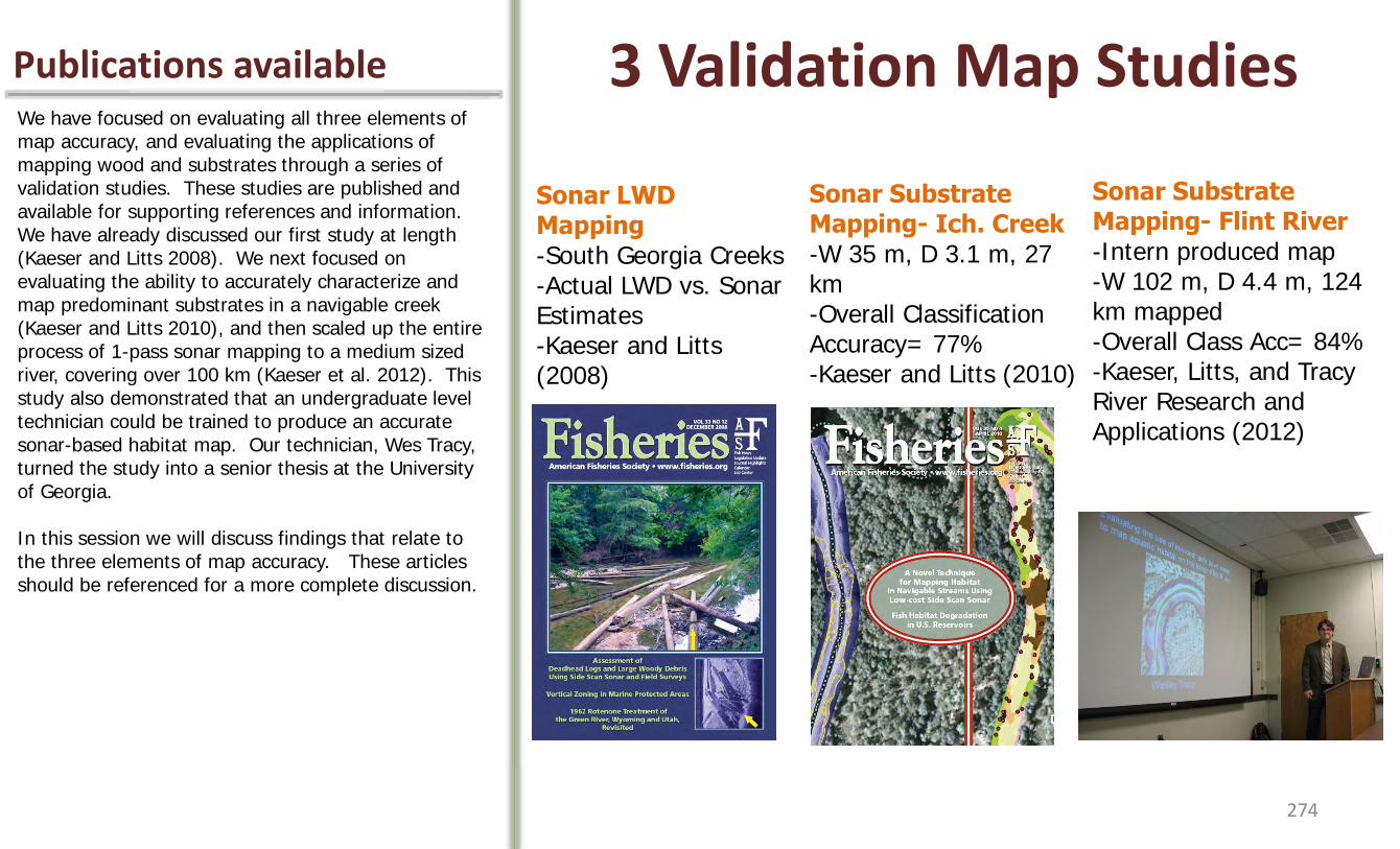
We have focused on evaluating all three elements of map accuracy, and evaluating the applications of mapping wood and substrates through a series of validation studies. These studies are published and available for supporting references and information. We have already discussed our first study at length (Kaeser and Litts 2008). We next focused on evaluating the ability to accurately characterize and map predominant substrates in a navigable creek (Kaeser and Litts 2010), and then scaled up the entire process of 1-pass sonar mapping to a medium sized river, covering over 100 km (Kaeser et al. 2012). This study also demonstrated that an undergraduate level technician could be trained to produce an accurate sonar-based habitat map. Our technician, Wes Tracy, turned the study into a senior thesis at the University of Georgia. In this session we will discuss findings that relate to the three elements of map accuracy. These articles should be referenced for a more complete discussion.

3 Validation Map Studies Publications available

Sonar LWD Mapping -South Georgia Creeks -Actual LWD vs. Sonar Estimates -Kaeser and Litts (2008)

Sonar Substrate Mapping- Ich. Creek -W 35 m, D 3.1 m, 27 km -Overall Classification Accuracy= 77% -Kaeser and Litts (2010)

Sonar Substrate Mapping- Flint River -Intern produced map -W 102 m, D 4.4 m, 124 km mapped -Overall Class Acc= 84% -Kaeser, Litts, and Tracy River Research and Applications (2012)

274

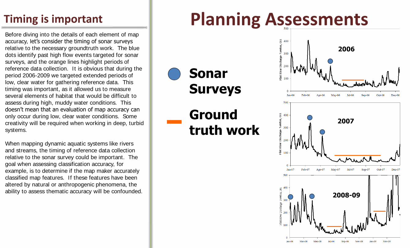
Before diving into the details of each element of map accuracy, let’s consider the timing of sonar surveys relative to the necessary groundtruth work. The blue dots identify past high flow events targeted for sonar surveys, and the orange lines highlight periods of reference data collection. It is obvious that during the period 2006-2009 we targeted extended periods of low, clear water for gathering reference data. This timing was important, as it allowed us to measure several elements of habitat that would be difficult to assess during high, muddy water conditions. This doesn’t mean that an evaluation of map accuracy can only occur during low, clear water conditions. Some creativity will be required when working in deep, turbid systems. When mapping dynamic aquatic systems like rivers and streams, the timing of reference data collection relative to the sonar survey could be important. The goal when assessing classification accuracy, for example, is to determine if the map maker accurately classified map features. If these features have been altered by natural or anthropogenic phenomena, the ability to assess thematic accuracy will be confounded.

Planning Assessments Timing is important

2006

2007

2008-09

Sonar Surveys

Ground truth work

When you need to visually assess substrate and count wood, conditions don’t get much better than this! During the drought of 2007, upstream portions of this creek ran dry. Here, in the lower reaches, infiltrating ground water turned the stream into what looked like a blue hole spring run. It hard to believe that during high flows this creek is among the most turbid in the region, with flow levels commonly reaching the top of the cut bank seen at the top and right of the photograph. Despite scorching summer temperatures, wetsuits were required to spend the whole day in the water collecting reference data. Here, Josh Hubbell floats over a large deadhead log. On the far side of the creek a limestone outcrop extends underwater to about mid-channel.

Spring Creek – Summer 2007 Benefits of a drought

276

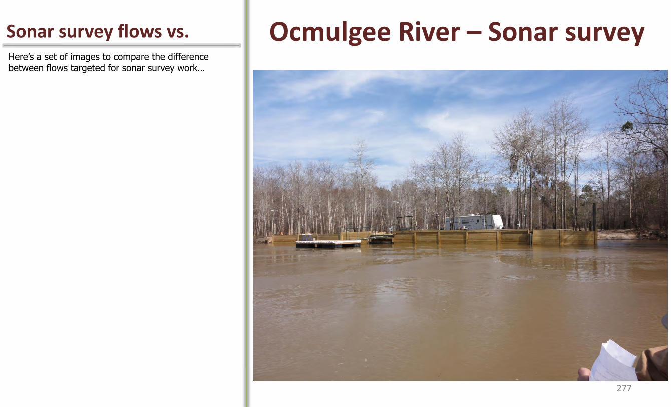
Here’s a set of images to compare the difference between flows targeted for sonar survey work…

Ocmulgee River – Sonar survey Sonar survey flows vs.

277

…and the flows targeted for reference data collection. Note the level of the floating dock in this photograph relative to the level during the sonar survey. Although this stream is not crystal clear, the clarity was sufficient to permit visual inspection of substrate in the shallows, and the use of a drop camera in deeper areas.

Ocmulgee River – Groundtruth Reference data collection

278

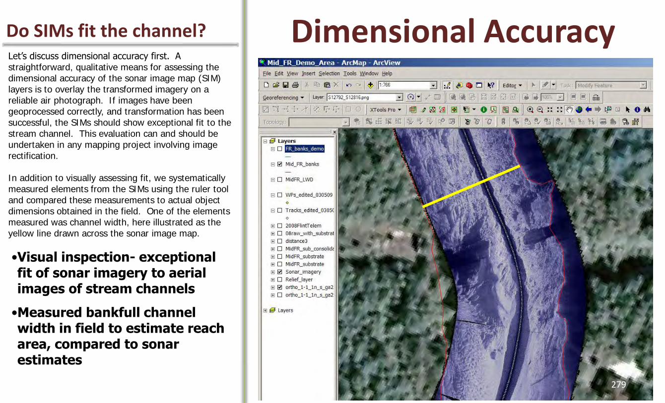
Let’s discuss dimensional accuracy first. A straightforward, qualitative means for assessing the dimensional accuracy of the sonar image map (SIM) layers is to overlay the transformed imagery on a reliable air photograph. If images have been geoprocessed correctly, and transformation has been successful, the SIMs should show exceptional fit to the stream channel. This evaluation can and should be undertaken in any mapping project involving image rectification. In addition to visually assessing fit, we systematically measured elements from the SIMs using the ruler tool and compared these measurements to actual object dimensions obtained in the field. One of the elements measured was channel width, here illustrated as the yellow line drawn across the sonar image map.

Dimensional Accuracy Do SIMs fit the channel?

•Visual inspection- exceptional fit of sonar imagery to aerial images of stream channels

•Measured bankfull channel width in field to estimate reach area, compared to sonar estimates

279

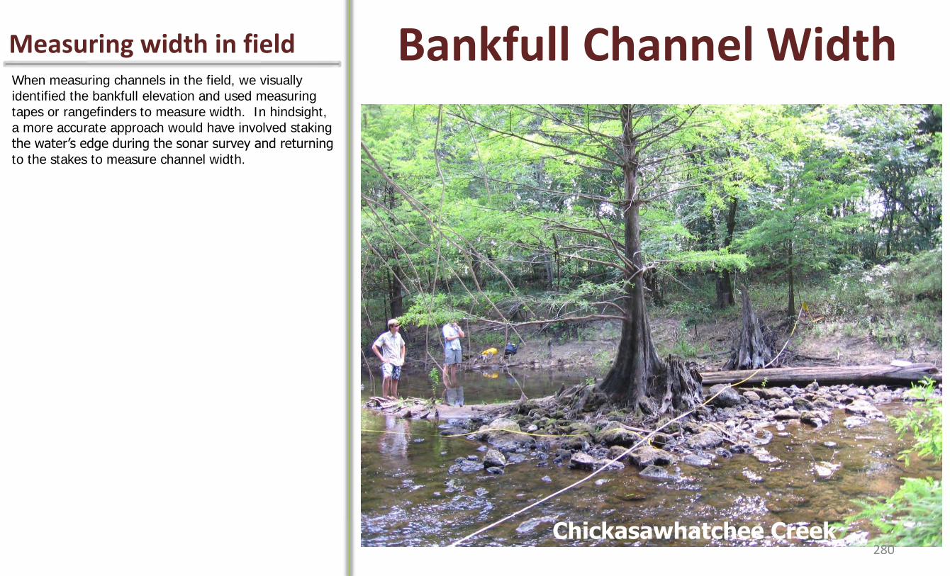
When measuring channels in the field, we visually identified the bankfull elevation and used measuring tapes or rangefinders to measure width. In hindsight, a more accurate approach would have involved staking the water’s edge during the sonar survey and returning to the stakes to measure channel width.

Bankfull Channel Width Measuring width in field

Chickasawhatchee Creek 280

Repeated cross-channel measurements of bankfull channel width were used in combination with reach length to estimate total reach area in several study reaches. These estimates were compared to reach area estimates made from the sonar image maps of the same reaches. Results indicated that sonar estimates of width were consistently greater than our field-based bankfull channel measurements. Sonar- based estimates of reach area were typically 10% greater than field estimates. One potential explanation for the discrepancy was that width of the stream channel during the sonar survey was slightly greater than the bankfull channel width measured in the field. At the time this study was conducted, slant range correction was not available for Humminbird imagery. The effect of slant range correction should be explored as an alternative explanation for the discrepancy.

Digitized stream banks approximate bankfull channel width

Measuring width in field

Reach area (ha) transect estimate

Line of equality y=x +20%

-20%

• Sonar channel width was consistently greater than field estimates of bankfull width

• One potential source for this discrepancy was width on survey date being greater than the bankfull width 281

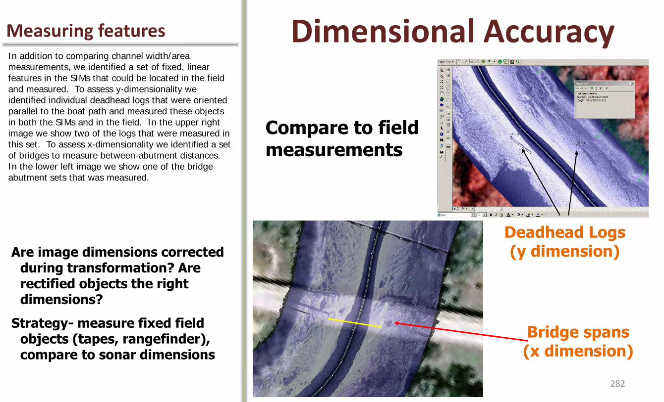
In addition to comparing channel width/area measurements, we identified a set of fixed, linear features in the SIMs that could be located in the field and measured. To assess y-dimensionality we identified individual deadhead logs that were oriented parallel to the boat path and measured these objects in both the SIMs and in the field. In the upper right image we show two of the logs that were measured in this set. To assess x-dimensionality we identified a set of bridges to measure between-abutment distances. In the lower left image we show one of the bridge abutment sets that was measured.

Dimensional Accuracy Measuring features

Are image dimensions corrected during transformation? Are rectified objects the right dimensions?

Strategy- measure fixed field objects (tapes, rangefinder), compare to sonar dimensions

Deadhead Logs (y dimension)

Bridge spans (x dimension)

Compare to field measurements

282

If rectification effectively corrects the dimensional distortion inherent in raw sonar imagery, we should find that measurements made from apparent objects/features in the sonar image maps would be nearly identical to the measurements obtained from these same objects in the field. Plotting sonar object length against actual object length in a scatterplot should reveal a series of points that fall along the line y=x; this is exactly what we found. Differences between measurements rarely exceeded 10% in either direction.

The results of the bridge span measurements were particularly encouraging in the sense that bridge abutments appeared in imagery that included the water column (no slant range correction performed). Given that the water column imposes some dimensional distortion to features in the near-field portion of the image (as previously discussed), we were encouraged to find that such distortion did not affect the apparent x-dimensionality of these objects. In other words, bridge abutments appeared in their proper place in the image, rather than farther apart as might be expected given the inclusion of the water column between abutments. (These results also support our supposition that differences between sonar survey water levels and bankfull channel levels in the field led to differences in sonar vs actual reach area estimates, rather than the use of imagery that included the water column).

Dimensional Accuracy Comparing measurements

Actual Object Length/Distance (m) 283

(Thom to Add)

Image Grid Measurements Transformed dimensions

Raw Image Grid dimensions based on .067m x .095 m pixel dimension (grid=100x100 pixels)

Transformed Image

Grid dimensions measured in ArcView

Note: Geoprocessing algorithm effectively corrected variably sized pixels 284

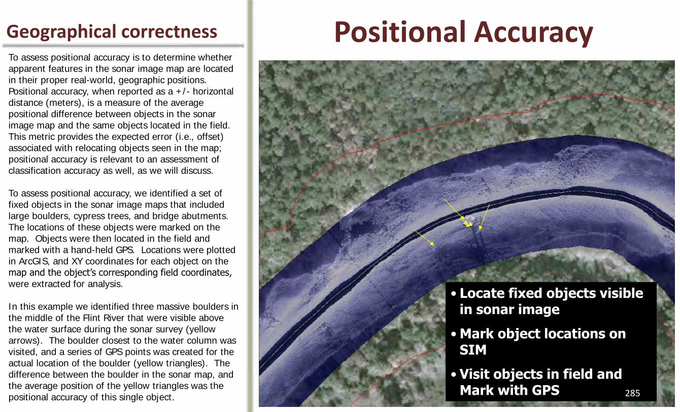
To assess positional accuracy is to determine whether apparent features in the sonar image map are located in their proper real-world, geographic positions. Positional accuracy, when reported as a +/- horizontal distance (meters), is a measure of the average positional difference between objects in the sonar image map and the same objects located in the field. This metric provides the expected error (i.e., offset) associated with relocating objects seen in the map; positional accuracy is relevant to an assessment of classification accuracy as well, as we will discuss. To assess positional accuracy, we identified a set of fixed objects in the sonar image maps that included large boulders, cypress trees, and bridge abutments. The locations of these objects were marked on the map. Objects were then located in the field and marked with a hand-held GPS. Locations were plotted in ArcGIS, and XY coordinates for each object on the map and the object’s corresponding field coordinates, were extracted for analysis. In this example we identified three massive boulders in the middle of the Flint River that were visible above the water surface during the sonar survey (yellow arrows). The boulder closest to the water column was visited, and a series of GPS points was created for the actual location of the boulder (yellow triangles). The difference between the boulder in the sonar map, and the average position of the yellow triangles was the positional accuracy of this single object.

Positional Accuracy Geographical correctness

• Locate fixed objects visible in sonar image

• Mark object locations on SIM

• Visit objects in field and Mark with GPS 285

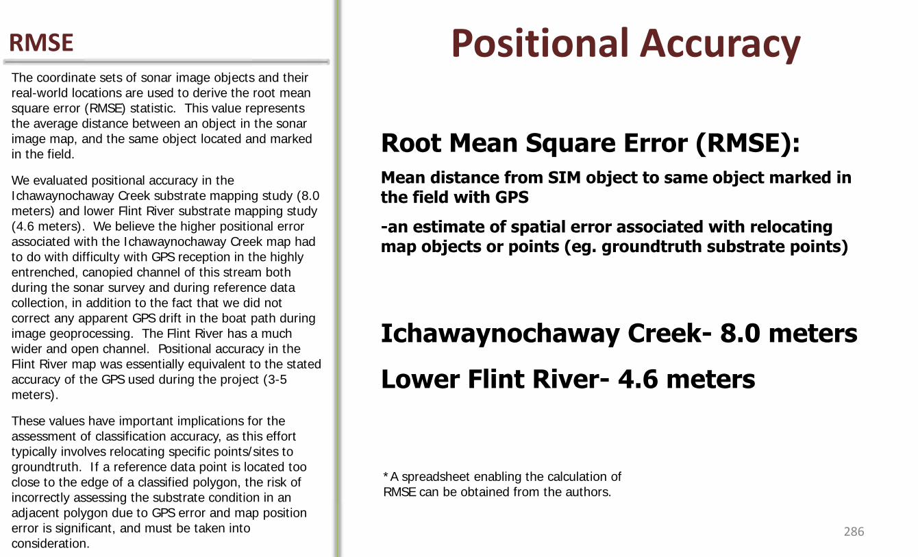
The coordinate sets of sonar image objects and their real-world locations are used to derive the root mean square error (RMSE) statistic. This value represents the average distance between an object in the sonar image map, and the same object located and marked in the field.

We evaluated positional accuracy in the Ichawaynochaway Creek substrate mapping study (8.0 meters) and lower Flint River substrate mapping study (4.6 meters). We believe the higher positional error associated with the Ichawaynochaway Creek map had to do with difficulty with GPS reception in the highly entrenched, canopied channel of this stream both during the sonar survey and during reference data collection, in addition to the fact that we did not correct any apparent GPS drift in the boat path during image geoprocessing. The Flint River has a much wider and open channel. Positional accuracy in the Flint River map was essentially equivalent to the stated accuracy of the GPS used during the project (3-5 meters).

These values have important implications for the assessment of classification accuracy, as this effort typically involves relocating specific points/sites to groundtruth. If a reference data point is located too close to the edge of a classified polygon, the risk of incorrectly assessing the substrate condition in an adjacent polygon due to GPS error and map position error is significant, and must be taken into consideration.

Positional Accuracy RMSE

Root Mean Square Error (RMSE):

Mean distance from SIM object to same object marked in the field with GPS

-an estimate of spatial error associated with relocating map objects or points (eg. groundtruth substrate points)

Ichawaynochaway Creek- 8.0 meters

Lower Flint River- 4.6 meters

*A spreadsheet enabling the calculation of RMSE can be obtained from the authors.

286

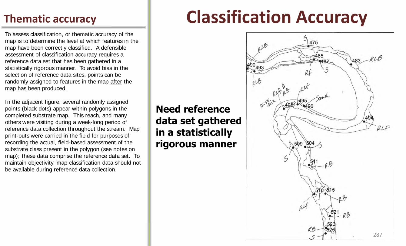
To assess classification, or thematic accuracy of the map is to determine the level at which features in the map have been correctly classified. A defensible assessment of classification accuracy requires a reference data set that has been gathered in a statistically rigorous manner. To avoid bias in the selection of reference data sites, points can be randomly assigned to features in the map after the map has been produced. In the adjacent figure, several randomly assigned points (black dots) appear within polygons in the completed substrate map. This reach, and many others were visiting during a week-long period of reference data collection throughout the stream. Map print-outs were carried in the field for purposes of recording the actual, field-based assessment of the substrate class present in the polygon (see notes on map); these data comprise the reference data set. To maintain objectivity, map classification data should not be available during reference data collection.

Classification Accuracy Thematic accuracy

Need reference data set gathered in a statistically rigorous manner

287

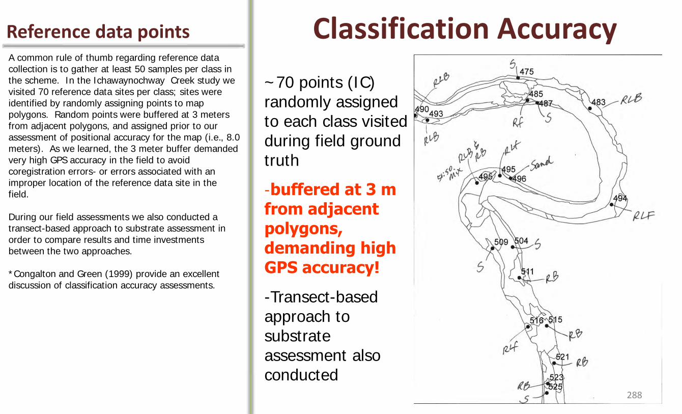
A common rule of thumb regarding reference data collection is to gather at least 50 samples per class in the scheme. In the Ichawaynochway Creek study we visited 70 reference data sites per class; sites were identified by randomly assigning points to map polygons. Random points were buffered at 3 meters from adjacent polygons, and assigned prior to our assessment of positional accuracy for the map (i.e., 8.0 meters). As we learned, the 3 meter buffer demanded very high GPS accuracy in the field to avoid coregistration errors- or errors associated with an improper location of the reference data site in the field. During our field assessments we also conducted a transect-based approach to substrate assessment in order to compare results and time investments between the two approaches. *Congalton and Green (1999) provide an excellent discussion of classification accuracy assessments.

Classification Accuracy Reference data points

~70 points (IC) randomly assigned to each class visited during field ground truth

-buffered at 3 m from adjacent polygons, demanding high GPS accuracy!

-Transect-based approach to substrate assessment also conducted

288

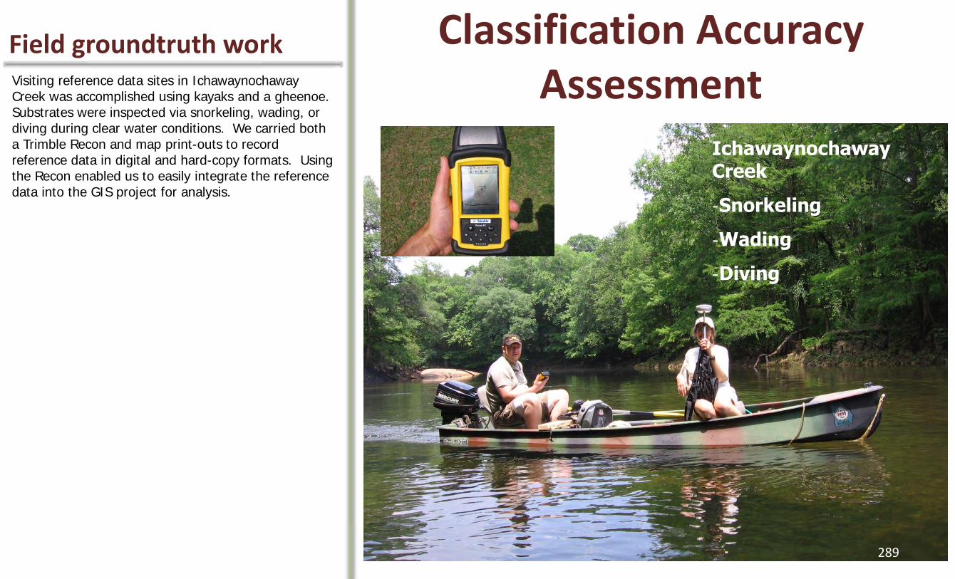
Visiting reference data sites in Ichawaynochaway Creek was accomplished using kayaks and a gheenoe. Substrates were inspected via snorkeling, wading, or diving during clear water conditions. We carried both a Trimble Recon and map print-outs to record reference data in digital and hard-copy formats. Using the Recon enabled us to easily integrate the reference data into the GIS project for analysis.

Classification Accuracy Assessment

Field groundtruth work


-Snorkeling

-Wading

-Diving

289

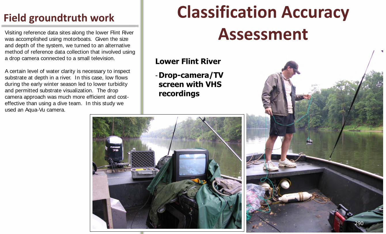
Visiting reference data sites along the lower Flint River was accomplished using motorboats. Given the size and depth of the system, we turned to an alternative method of reference data collection that involved using a drop camera connected to a small television. A certain level of water clarity is necessary to inspect substrate at depth in a river. In this case, low flows during the early winter season led to lower turbidity and permitted substrate visualization. The drop camera approach was much more efficient and cost-effective than using a dive team. In this study we used an Aqua-Vu camera.

Classification Accuracy Assessment

Field groundtruth work


-Snorkeling

-Wading

-Diving

Lower Flint River

-Drop-camera/TV screen with VHS recordings

290

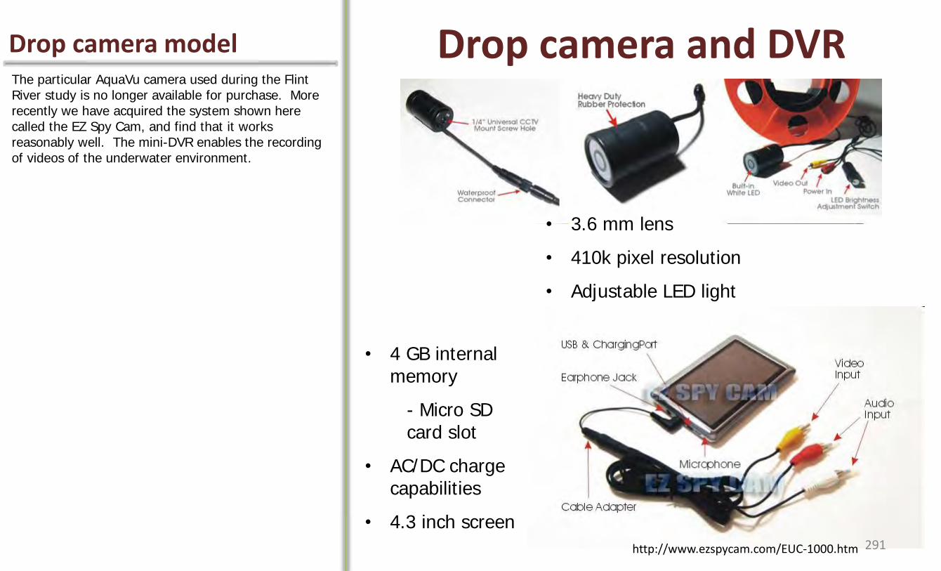
The particular AquaVu camera used during the Flint River study is no longer available for purchase. More recently we have acquired the system shown here called the EZ Spy Cam, and find that it works reasonably well. The mini-DVR enables the recording of videos of the underwater environment.

Drop camera and DVR Drop camera model

• 3.6 mm lens

• 410k pixel resolution

• Adjustable LED light

• 4 GB internal memory

- Micro SD card slot

• AC/DC charge capabilities

• 4.3 inch screen

http://www.ezspycam.com/EUC-1000.htm 291

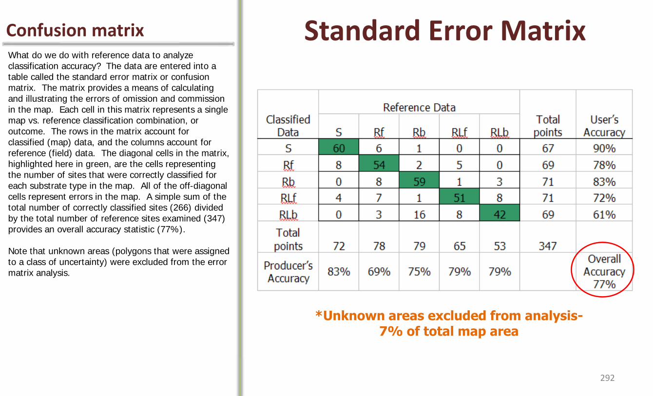
What do we do with reference data to analyze classification accuracy? The data are entered into a table called the standard error matrix or confusion matrix. The matrix provides a means of calculating and illustrating the errors of omission and commission in the map. Each cell in this matrix represents a single map vs. reference classification combination, or outcome. The rows in the matrix account for classified (map) data, and the columns account for reference (field) data. The diagonal cells in the matrix, highlighted here in green, are the cells representing the number of sites that were correctly classified for each substrate type in the map. All of the off-diagonal cells represent errors in the map. A simple sum of the total number of correctly classified sites (266) divided by the total number of reference sites examined (347) provides an overall accuracy statistic (77%). Note that unknown areas (polygons that were assigned to a class of uncertainty) were excluded from the error matrix analysis.

Standard Error Matrix Confusion matrix

*Unknown areas excluded from analysis- 7% of total map area

292

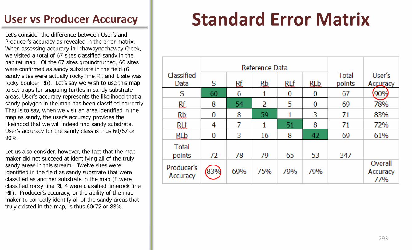
Let’s consider the difference between User’s and Producer’s accuracy as revealed in the error matrix. When assessing accuracy in Ichawaynochaway Creek, we visited a total of 67 sites classified sandy in the habitat map. Of the 67 sites groundtruthed, 60 sites were confirmed as sandy substrate in the field (6 sandy sites were actually rocky fine Rf, and 1 site was rocky boulder Rb). Let’s say we wish to use this map to set traps for snapping turtles in sandy substrate areas. User’s accuracy represents the likelihood that a sandy polygon in the map has been classified correctly. That is to say, when we visit an area identified in the map as sandy, the user’s accuracy provides the likelihood that we will indeed find sandy substrate. User’s accuracy for the sandy class is thus 60/67 or 90%. Let us also consider, however, the fact that the map maker did not succeed at identifying all of the truly sandy areas in this stream. Twelve sites were identified in the field as sandy substrate that were classified as another substrate in the map (8 were classified rocky fine Rf, 4 were classified limerock fine Rlf). Producer’s accuracy, or the ability of the map maker to correctly identify all of the sandy areas that truly existed in the map, is thus 60/72 or 83%.

Standard Error Matrix User vs Producer Accuracy

293

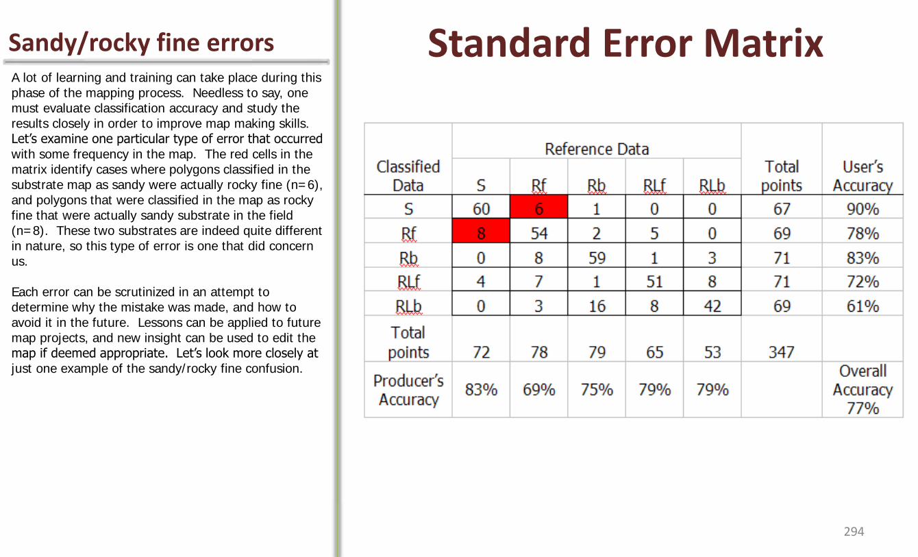
A lot of learning and training can take place during this phase of the mapping process. Needless to say, one must evaluate classification accuracy and study the results closely in order to improve map making skills. Let’s examine one particular type of error that occurred with some frequency in the map. The red cells in the matrix identify cases where polygons classified in the substrate map as sandy were actually rocky fine (n=6), and polygons that were classified in the map as rocky fine that were actually sandy substrate in the field (n=8). These two substrates are indeed quite different in nature, so this type of error is one that did concern us. Each error can be scrutinized in an attempt to determine why the mistake was made, and how to avoid it in the future. Lessons can be applied to future map projects, and new insight can be used to edit the map if deemed appropriate. Let’s look more closely at just one example of the sandy/rocky fine confusion.

Standard Error Matrix Sandy/rocky fine errors

294

In this example, we visited a small polygon along the margin of the creek that was classified as sandy substrate in the map. Note that this small polygon was bounded by an outcrop of limerock boulder in upstream and downstream directions.

Example of misclassified polygon

Polygon classified sandy

This polygon (70 m2)

classified Sandy

295

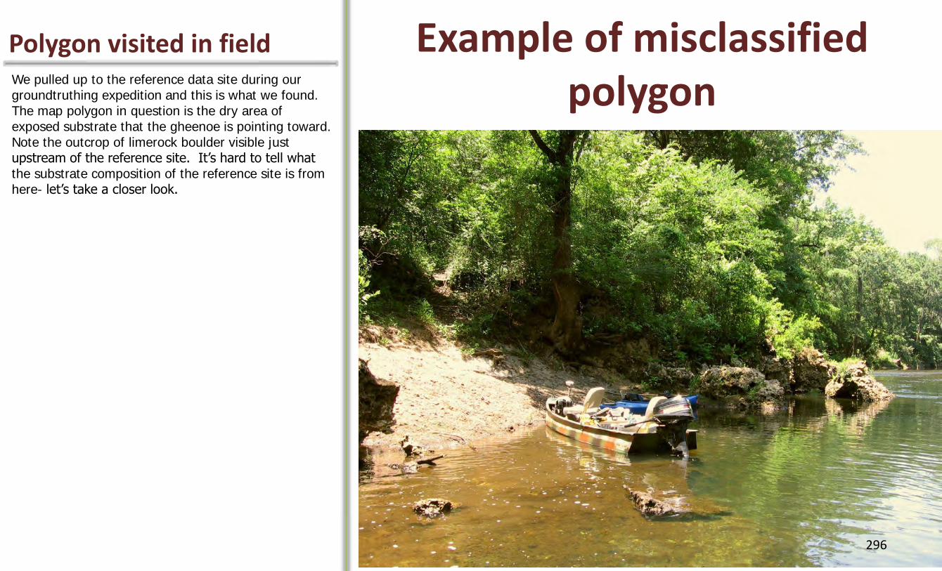
We pulled up to the reference data site during our groundtruthing expedition and this is what we found. The map polygon in question is the dry area of exposed substrate that the gheenoe is pointing toward. Note the outcrop of limerock boulder visible just upstream of the reference site. It’s hard to tell what the substrate composition of the reference site is from here- let’s take a closer look.

Example of misclassified polygon

Polygon visited in field

296

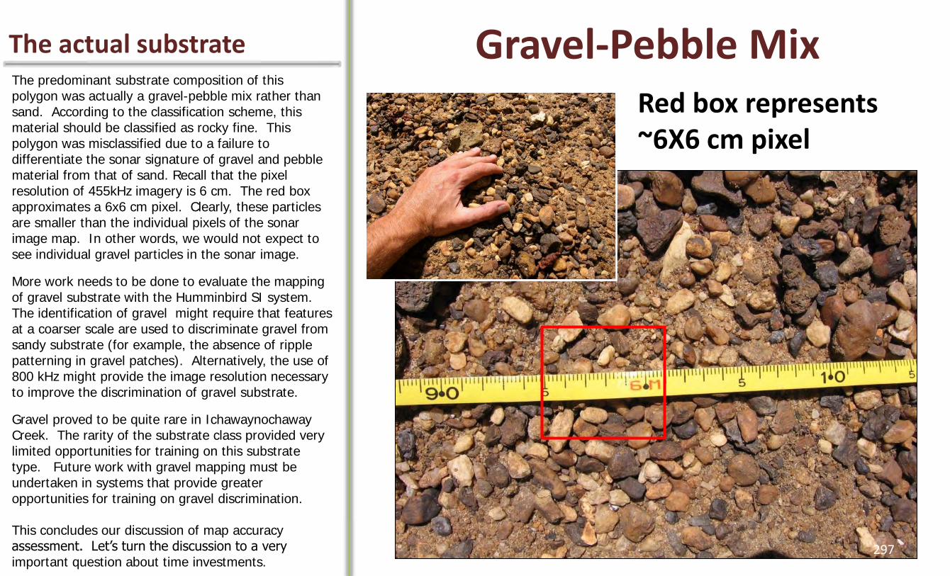
The predominant substrate composition of this polygon was actually a gravel-pebble mix rather than sand. According to the classification scheme, this material should be classified as rocky fine. This polygon was misclassified due to a failure to differentiate the sonar signature of gravel and pebble material from that of sand. Recall that the pixel resolution of 455kHz imagery is 6 cm. The red box approximates a 6x6 cm pixel. Clearly, these particles are smaller than the individual pixels of the sonar image map. In other words, we would not expect to see individual gravel particles in the sonar image.

More work needs to be done to evaluate the mapping of gravel substrate with the Humminbird SI system. The identification of gravel might require that features at a coarser scale are used to discriminate gravel from sandy substrate (for example, the absence of ripple patterning in gravel patches). Alternatively, the use of 800 kHz might provide the image resolution necessary to improve the discrimination of gravel substrate.

Gravel proved to be quite rare in Ichawaynochaway Creek. The rarity of the substrate class provided very limited opportunities for training on this substrate type. Future work with gravel mapping must be undertaken in systems that provide greater opportunities for training on gravel discrimination. This concludes our discussion of map accuracy assessment. Let’s turn the discussion to a very important question about time investments.

Gravel-Pebble Mix The actual substrate

Red box represents ~6X6 cm pixel

297

How much time does this whole process of habitat mapping require? Over several mapping projects we have maintained records of time invested during various steps of the mapping process. Along the way, Thom completed several improvements to the GIS Sonar Toolkit that involve automation of processing steps, further reducing time investments. A transect-based approach to substrate assessment required 24+ man hours per kilometer for us to complete. This approach assessed only the coverage of substrates along transects spaced at 20-meter intervals. In many places, this approach will not be feasible due to size, depth, and turbidity. In contrast, the entire sonar-based approach to mapping habitat required only 2-3 hours per kilometer to complete. The specific length of time will vary depending on the complexity and size of the system, in addition to the variety of elements being mapped. These estimates included the mapping of large woody debris, a very time intensive step of the process. Nonetheless, the sonar-based approach represents the time savings of an order of magnitude to project completion. Moreover, the sonar habitat map, unlike the transect-based assessment, provides complete bank-to-bank spatial coverage- a complete census of the entire study area is provided.

How much time? Time investments

Transect-based approach = 24+ hrs/km

Sonar-based approach = 2-3 hrs/km

VS

298

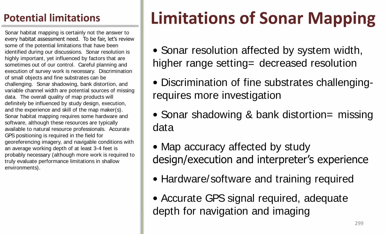
Sonar habitat mapping is certainly not the answer to every habitat assessment need. To be fair, let’s review some of the potential limitations that have been identified during our discussions. Sonar resolution is highly important, yet influenced by factors that are sometimes out of our control. Careful planning and execution of survey work is necessary. Discrimination of small objects and fine substrates can be challenging. Sonar shadowing, bank distortion, and variable channel width are potential sources of missing data. The overall quality of map products will definitely be influenced by study design, execution, and the experience and skill of the map maker(s). Sonar habitat mapping requires some hardware and software, although these resources are typically available to natural resource professionals. Accurate GPS positioning is required in the field for georeferencing imagery, and navigable conditions with an average working depth of at least 3-4 feet is probably necessary (although more work is required to truly evaluate performance limitations in shallow environments).

Limitations of Sonar Mapping Potential limitations

• Sonar resolution affected by system width, higher range setting= decreased resolution

• Discrimination of fine substrates challenging- requires more investigation

• Sonar shadowing & bank distortion= missing data

• Map accuracy affected by study design/execution and interpreter’s experience

• Hardware/software and training required

• Accurate GPS signal required, adequate depth for navigation and imaging

299

On the other hand, low-cost sonar habitat mapping provides a rapid, accurate, flexible, and inexpensive means to map and quantify elements of physical habitat and other features in turbid, non-wadeable streams at the landscape scale. Side scan sonar has been around for 50+ years, yet the business of mapping habitat in inland waters has simply not become commonplace- Why? We believe the reason is lack of access to low-cost equipment, tools, and training. Indeed, a major goal of the sonar habitat mapping initiative is to provide the tools and training to overcome this hurdle. We hope that this guidebook and the tools that accompany it contribute significantly toward this effort.

Benefits of Sonar Mapping Why sonar mapping?

Lower Flint River

• Rapid, accurate, flexible, & inexpensive means to map and quantify habitat in turbid, non-wadeable systems at landscape scale

300

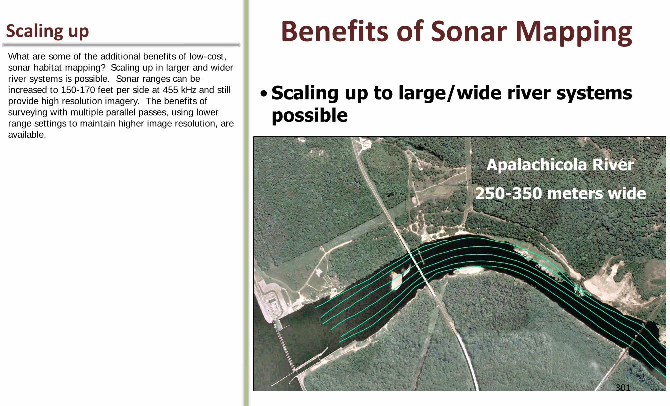
What are some of the additional benefits of low-cost, sonar habitat mapping? Scaling up in larger and wider river systems is possible. Sonar ranges can be increased to 150-170 feet per side at 455 kHz and still provide high resolution imagery. The benefits of surveying with multiple parallel passes, using lower range settings to maintain higher image resolution, are available.

Benefits of Sonar Mapping Scaling up

Lower Flint River

• Scaling up to large/wide river systems possible

Apalachicola River

250-350 meters wide

301

Another major benefit is that sonar based habitat maps can applied to ecological research, conservation planning and design, and monitoring. The map is a tool, and it should be put to good use!

Since sonar habitat maps are produced within a GIS platform, spatial biological data can easily be integrated and linked to physical habitat, unlocking a trove of potential analyses. This integration enables studies of organism-habitat associations and behavioral patterns at the landscape scale. Given the availability of terrestrial data layers, the associations between landuse and physical aquatic habitat can also be explored.

Fortunately for us, terrestrial ecologists have been developing landscape level approaches to analyzing organism-habitat relationships for some time now. A robust field of research and publications is available for mining ideas and models. Now that the tools and techniques are available to fill the aquatic habitat gap, it’s time to take landscape ecology to the water!

Applications Integrating biological data

Lower Flint River

• Sonar habitat maps can be integrated with other spatial datasets to yield great analysis potential

- Studies of organism-habitat associations and behavioral patterns

- Landuse/landcover associations with instream habitat

• Monitoring habitat change over time

*These figures from the study – Goclowski M.R., A. J. Kaeser, and S. M. Sammons (2012). Movement and habitat differentiation among adult shoal bass, largemouth bass, and spotted bass in the upper Flint River, Georgia. North American Journal of Fisheries Management. 302

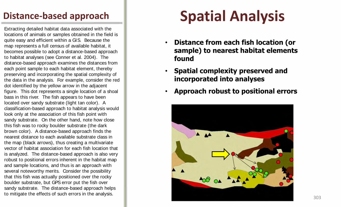
Extracting detailed habitat data associated with the locations of animals or samples obtained in the field is quite easy and efficient within a GIS. Because the map represents a full census of available habitat, it becomes possible to adopt a distance-based approach to habitat analyses (see Conner et al. 2004). The distance-based approach examines the distances from each point sample to each habitat element, thereby preserving and incorporating the spatial complexity of the data in the analysis. For example, consider the red dot identified by the yellow arrow in the adjacent figure. This dot represents a single location of a shoal bass in this river. The fish appears to have been located over sandy substrate (light tan color). A classification-based approach to habitat analysis would look only at the association of this fish point with sandy substrate. On the other hand, note how close this fish was to rocky boulder substrate (the dark brown color). A distance-based approach finds the nearest distance to each available substrate class in the map (black arrows), thus creating a multivariate vector of habitat association for each fish location that is analyzed. The distance-based approach is also very robust to positional errors inherent in the habitat map and sample locations, and thus is an approach with several noteworthy merits. Consider the possibility that this fish was actually positioned over the rocky boulder substrate, but GPS error put the fish over sandy substrate. The distance-based approach helps to mitigate the effects of such errors in the analysis.

Spatial Analysis Distance-based approach

Lower Flint River

• Distance from each fish location (or sample) to nearest habitat elements found

• Spatial complexity preserved and incorporated into analyses

• Approach robust to positional errors

303

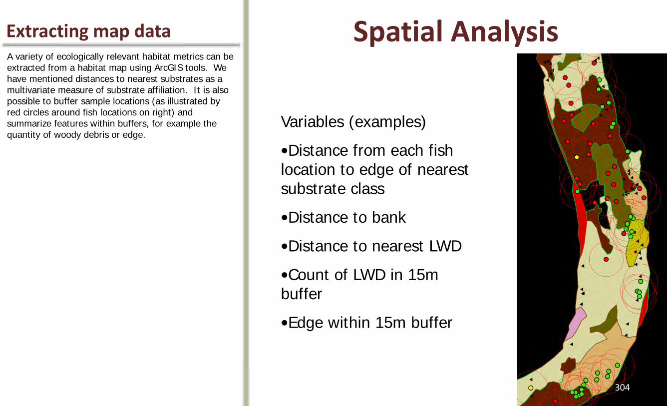
A variety of ecologically relevant habitat metrics can be extracted from a habitat map using ArcGIS tools. We have mentioned distances to nearest substrates as a multivariate measure of substrate affiliation. It is also possible to buffer sample locations (as illustrated by red circles around fish locations on right) and summarize features within buffers, for example the quantity of woody debris or edge.

Spatial Analysis Extracting map data

Lower Flint River

Variables (examples)

•Distance from each fish location to edge of nearest substrate class

•Distance to bank

•Distance to nearest LWD

•Count of LWD in 15m buffer

•Edge within 15m buffer

304

Like any air photo or lidar data set, the sonar image map represents a snapshot in time. Sonar mapping can be applied in a time-lapse fashion (i.e., multiple surveys over time) to monitor and study potential changes in habitat. Just as a forest ecologist studies decadal trends in forest composition, why not examine trends in substrate composition of the riverbed? What might we learn? We’ve only just begun to casually look at how substrate composition can change over time in some of the rivers we frequent. In some cases, the changes are quite striking. The example provided here comes from a pair of surveys covering a reach of the Altamaha River. On the left side of the image we find a group of large boulder-like hard substrates (rock or hard clay). Downstream of this outcrop is the leading edge of a massive sand wave or dune, outlined by the dashed yellow line. Further downstream is an area along the right bank that has cobble sized rock or clay composition, barely visible at this scale. This image was produced February 1, 2011. *The fundamental goal of this project was to identify the limited occurrences of hard bottom substrate available as potential spawning habitat for sturgeon, not the documentation of change over time.

Applications Study change over time

Lower Flint River

Quantifying changes in habitat

Surveyed 2/1/11

305

Three weeks later this reach was resurveyed. Some impressive changes had occurred to substrate composition. The clay outcrop/boulder area in the upper left had been scoured clean of some sand, and the massive sand wave from February 1 had vanished. The sand appears to have been transported and deposited approximately 150 meters downstream of its former location, where it now smothers the area of cobble-sized material along the right bank. These changes were associated with a runoff event that occurred between surveys (see hydrograph below).

Aquatic systems will likely change at varying rates, and in response to unpredictable events. Does this negate sonar mapping- of course not! Our world is constantly changing, yet we rely on maps all the time. The potential for change should be considered when producing and applying sonar map products.

Applications Change over time

Lower Flint River

…3 weeks later (02/23/11)

150 meter shift

* Flood stage is ~90,000 cfs for the gauge location, so the runoff event associated with this change was not a flood.

306

Quantifying changes in habitat

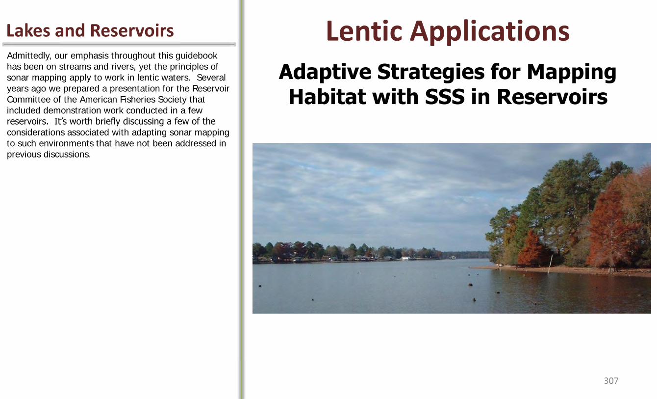
Admittedly, our emphasis throughout this guidebook has been on streams and rivers, yet the principles of sonar mapping apply to work in lentic waters. Several years ago we prepared a presentation for the Reservoir Committee of the American Fisheries Society that included demonstration work conducted in a few reservoirs. It’s worth briefly discussing a few of the considerations associated with adapting sonar mapping to such environments that have not been addressed in previous discussions.

Lentic Applications Lakes and Reservoirs

Lower Flint River

Adaptive Strategies for Mapping Habitat with SSS in Reservoirs

307

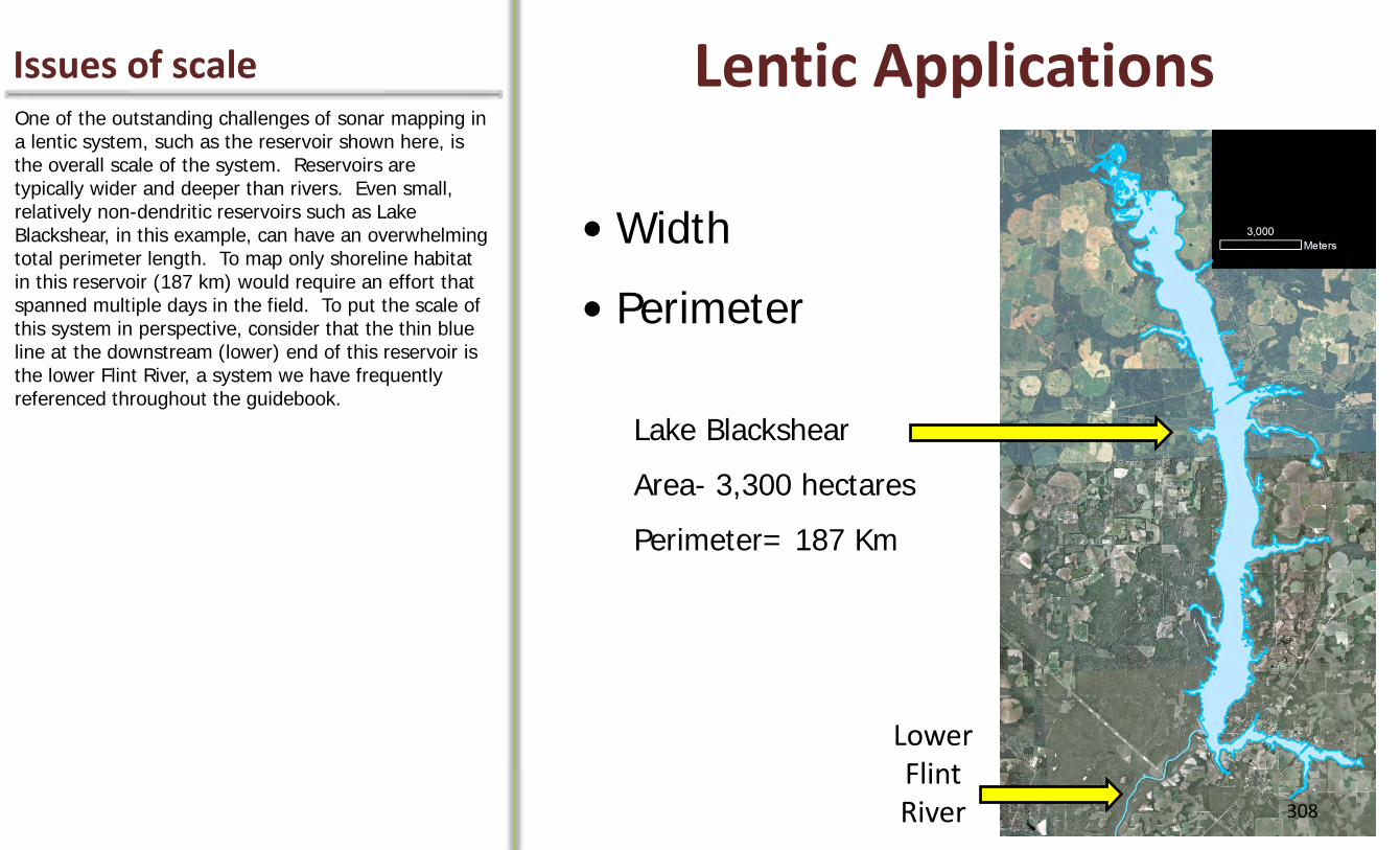
One of the outstanding challenges of sonar mapping in a lentic system, such as the reservoir shown here, is the overall scale of the system. Reservoirs are typically wider and deeper than rivers. Even small, relatively non-dendritic reservoirs such as Lake Blackshear, in this example, can have an overwhelming total perimeter length. To map only shoreline habitat in this reservoir (187 km) would require an effort that spanned multiple days in the field. To put the scale of this system in perspective, consider that the thin blue line at the downstream (lower) end of this reservoir is the lower Flint River, a system we have frequently referenced throughout the guidebook.

Lentic Applications Issues of scale

Lower Flint River

• Width

• Perimeter

Lake Blackshear

Area- 3,300 hectares

Perimeter= 187 Km


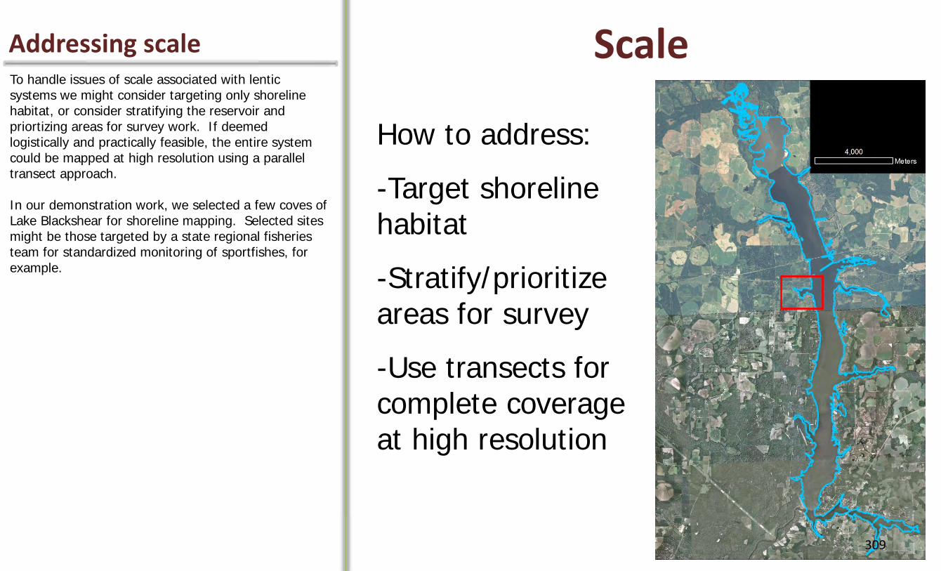
Scale Addressing scale

Lower Flint River

How to address:

-Target shoreline habitat

-Stratify/prioritize areas for survey

-Use transects for complete coverage at high resolution

To handle issues of scale associated with lentic systems we might consider targeting only shoreline habitat, or consider stratifying the reservoir and priortizing areas for survey work. If deemed logistically and practically feasible, the entire system could be mapped at high resolution using a parallel transect approach. In our demonstration work, we selected a few coves of Lake Blackshear for shoreline mapping. Selected sites might be those targeted by a state regional fisheries team for standardized monitoring of sportfishes, for example.

309

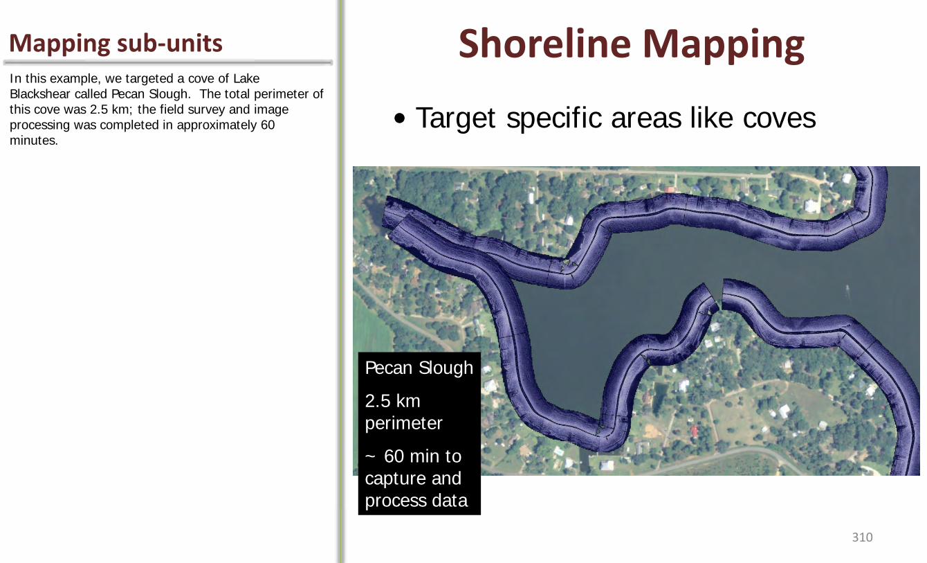
Shoreline Mapping Mapping sub-units

Lower Flint River

In this example, we targeted a cove of Lake Blackshear called Pecan Slough. The total perimeter of this cove was 2.5 km; the field survey and image processing was completed in approximately 60 minutes.

Pecan Slough

2.5 km perimeter

~ 60 min to capture and process data

• Target specific areas like coves

310

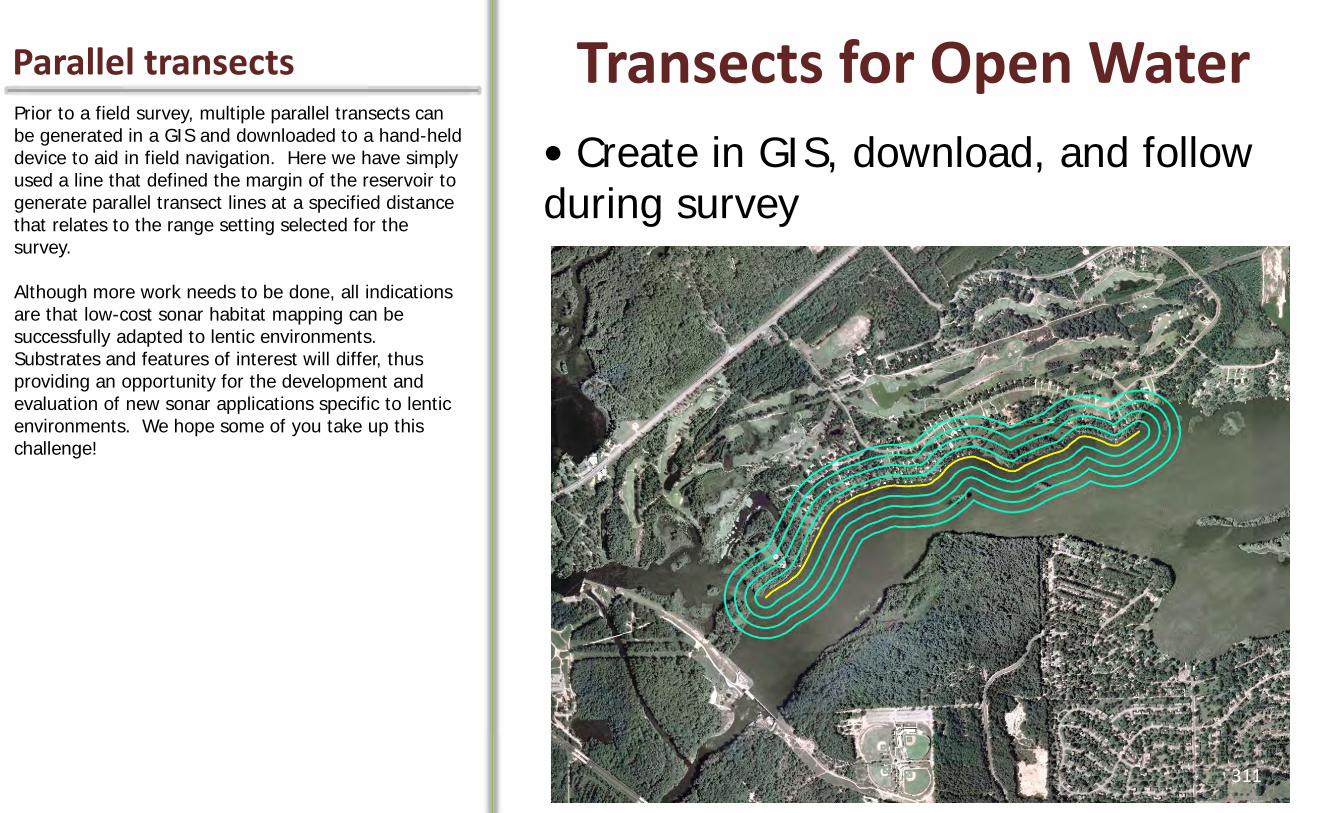
Transects for Open Water Parallel transects

Lower Flint River

Prior to a field survey, multiple parallel transects can be generated in a GIS and downloaded to a hand-held device to aid in field navigation. Here we have simply used a line that defined the margin of the reservoir to generate parallel transect lines at a specified distance that relates to the range setting selected for the survey. Although more work needs to be done, all indications are that low-cost sonar habitat mapping can be successfully adapted to lentic environments. Substrates and features of interest will differ, thus providing an opportunity for the development and evaluation of new sonar applications specific to lentic environments. We hope some of you take up this challenge!

• Create in GIS, download, and follow during survey

311

The Future of the Initiative Where do we go from here

Lower Flint River

We are fortunate and grateful to have had the resources, support, and opportunities required to successfully accomplish many of the original objectives of the sonar habitat mapping initiative. We continue to offer training, and develop supporting materials, and now currently work toward the development and evaluation of new sonar mapping applications and applied studies, several of which are listed here. We hope that these studies continue to build the foundation necessary for widespread adoption and implementation of this promising methodology. As always, please feel free to contact us with questions or comments, and provide feedback on your experiences with low-cost sonar habitat mapping. We would be glad to provide any assistance possible. We hope that this Guidebook and the attendant materials successfully serve our stated purpose of providing you with a quick-start guide to low-cost sonar habitat mapping. Please share these materials with others, and may you find the enlightening experience of sonar mapping well within your grasp. We’ll leave you with just of few more photographs of our work on sonar mapping…Thanks to all of our field asssistants, interns, and supporters!

Application studies/projects underway

• Habitat selection of female Barbour’s map turtle in a Southwest GA creek (S. Sterret, in preparation)

• Using time-lapse sonar habitat mapping to assess changes in substrate deposition following a 10-year flood event (A. Crawford, MS student)

• GA Altamaha Basin mapping project (sturgeon) (T. Litts/GADNR)

• Apalachicola River Applied Mapping project- modeling the distribution and abundance of mussels in a large, meandering river (R. Smit, MS student Auburn/USFWS)

• Development and evaluation of a sonar-based approach to monitoring distribution and abundance of adult Gulf sturgeon (A. Kaeser/USFWS)

• A performance evaluation of 2 side scan systems for detecting Gulf sturgeon (USFWS/USGS/NCState/Delaware State University)

• Evaluation of alligator snapping turtle habitat use in the Suwannee River via telemetry and sonar mapping (T. Thomas, FWC/U Florida, USFWS)

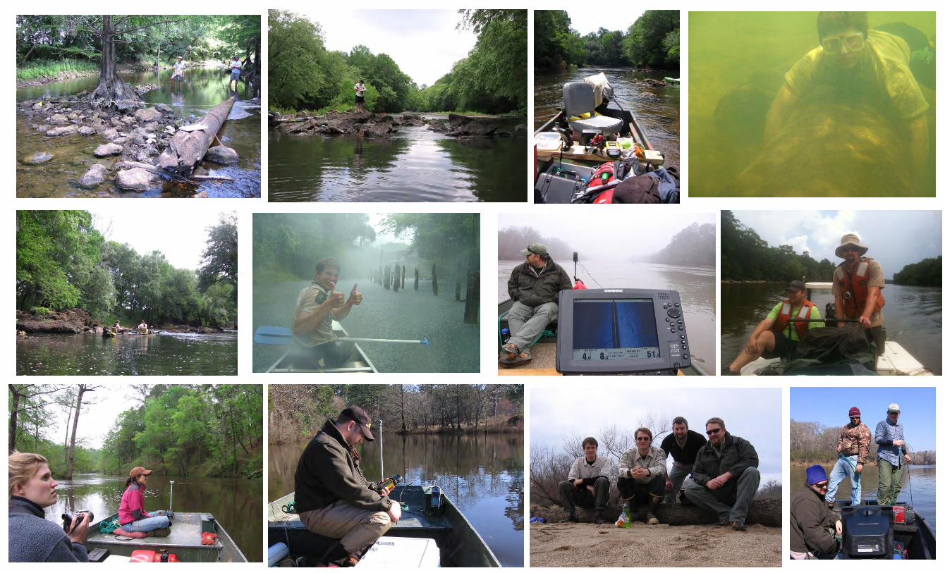
Lower Flint River

Additional References

Lower Flint River

314

Congalton, R. G., and K. Green. 1999. Assessing the accuracy of classification of remotely sensed data: principles and practices. Lewis Publishers, New York. Goclowski, M. R., A. J. Kaeser, and S. M. Sammons. 2012. Movement and habitat differentiation among shoal bass, largemouth bass, and spotted bass in the upper Flint River, Georgia. North American Journal of Fisheries Management. DOI:10.1080/02755947.2012.741555. Kaeser, A. J. and T. L. Litts. 2013. Sonar Image Geoprocessing Workbook- An illustrated guide to geoprocessing low-cost, side scan sonar imagery obtained with the Humminbird® Side Imaging System. Version 2.1. Georgia Department of Natural Resources, Social Circle, GA. U.S. Fish and Wildlife Service, Panama City Fish and Wildlife Conservation Office, Panama City, Florida. Kaeser, A. J., T. L. Litts, and T. W. Tracy. 2012. Using low-cost side scan sonar for benthic mapping throughout the lower Flint River, Georgia, USA. River Research and Applications. DOI:10.1002/rra.2556. Kaeser, A. J. and T. L. Litts. 2010. A novel technique for mapping habitat in navigable streams using low-cost side scan sonar. Fisheries 35(4):163-174. Kaeser, A. J. and T. L. Litts. 2008. An assessment of deadhead logs and large woody debris using side scan sonar and field surveys in streams of Southwest Georgia. Fisheries 33(12):589-597.

Documents

An Illustrated Guide to Low-cost, Side Scan Sonar Habitat Mapping