Embed Size (px)
Citation preview

An Extended Scalar Sector:Charged Higgs and Dark Matter
Mahdi Poormohammadi
Dissertation for the degree of Philosophy Doctor (PhD)
Department of Physics and Technology
University of Bergen
June 2013

2

Acknowledgements
In carrying out my study I am indebted to many people, including my teachers, col-leagues and friends. The first and the most, I would like to thank my supervisor pro-fessor Per Osland, who provided me with the concept for this thesis, for his academicaland partially financial support throughout my study. Without his help and instructions,I would not be able to complete this thesis.
Acknowledgments are also given to the Norwegian Research Council for partialfinancial support.
I also would like to extend my gratefulness to my co-supervisors, professor AnnaLipniacka at the University of Bergen and Dr. Odd Magne Ogreid at Bergen College.
I have been aided by several individuals. Dr. Marco Pruna has generously providedsupport both in developing and implementing our model in CalcHEP and giving me theopportunity to interact and work with him. My words can certainly not express howmuch he has been beneficial to me in my studies. Dr. Florian Bonnet has been thesource of invaluable information about the code MadEvent. Even though I have nevermet him in my life, he has been replying to my emails promptly and patiently. I wouldlike to thank Dr. Nils-Erik Bomark with whom I shared my office and who was alwaysavailable to answer my questions.
I am extremely grateful about the atmosphere prevalent in the Department ofPhysics and Technology. I scientifically benefited from all people on the third floor.
Some moments are so dumb that one could not even share them with one’s parents,but God has created friendship and friends for these moments. In this regard, I thankSirus Seraji and his kind family. My thankfulness likewise extends to all my friends fortheir encouragements and understanding in my odd hours.
My special thanks go to Barbara for her being very patient during the last 3 yearsand her trying to be supportive. Furthermore, I am deeply indebted to my family andparents. Their love is always supportive, encouraging and invaluable with no expecta-tion! They never became displeased even though I could only meet them once in a longwhile!
I thank the Journal of High Energy Physics for allowing me to use the papers in thethesis.
Mahdi Purmohammadi

ii Acknowledgements

Abstract
Despite the great success of the Standard Model in describing many aspects of the ex-periments, there are compelling reasons that it needs to be improved. One of the majormysteries physics has been exploring is the composition of matter in the Universe. Thedensity of the luminous matter Ωlum is thought to be about 4% of the total energy den-sity Ωtot of the Universe. Dark Matter makes up ∼ 26% of the energy density of theUniverse which is inferred by its gravitational effects and bending of light from lu-minous matter as well as the geometry of the Universe. Over the last few years theparadigm of DM has shifted towards the subatomic Weakly Interacting Massive Par-ticles (WIMPs). Thus, the existence of DM is one of the most important pieces ofevidence for physics Beyond the Standard Model (BSM). The observation of DM willpresumably indicate that there is a new particle.
The discovery of the Higgs particle paves the way beyond the SM for exploringthe existence of new particles and the component of dark matter. There are severalattempts to extend the SM and include the new physics. The Two-Higgs-Doublet Model(2HDM) is one of those. This model offers a new spectrum of scalar particles. Theseparticles can accommodate additional CP violation in the neutral sector of the Higgspotential. These particles can be produced at accelerators. If they are produced, theywill decay to SM particles via a chain of decay modes. Their signals can be discernedagainst the SM background, by means of a set of feasible techniques. From this point ofview, one good avenue in search for physics beyond the SM is to search for new chargedparticles. In the context of the 2HDM, the charged Higgs bosons can be produced inassociation with quarks, neutral Higgs bosons and the W bosons. The production rateof the charged Higgs bosons along with the neutral Higgs bosons is too low to give riseto visible signals over the SM background. But the other channels hold promises. Inparticular, the event analysis of the charged Higgs boson produced in association withthe W boson leads to a number of surviving signal events after passing a set of filters.
There are also extensions to the SM that accommodate a DM candidate. Let usconsider the 2HDM extension of the SM model. The 2HDM could be equipped withan extra doublet which is inert in the sense that it has zero vacuum expectation valueand does not couple to fermions. Therefore the resulting model is refereed to as CP-violating Inert Doublet Model (or IDM2). The lightest neutral member of the model,by help of an ad hoc Z2 symmetry, is stabilized to contribute to the missing mass of theUniverse.
The IDM2 is viable in two different mass domains of the DM candidate, namelylow and high mass regions. The model can naturally reproduce the observed DM abun-dance due to effective DM self-annihilation in the early Universe in the low-mass regionwhich is within reach of the LHC experiments at CERN. These experiments might il-luminate our understanding of the nature of the DM. Besides, parameter points in the

iv Abstract
low mass region pass the constraints from the latest experiments in search for DM bothin direct and indirect ones. Due to the nature of the imposed symmetry, the membersof the inert doublet will be produced in pairs. In a suitable part of the parameter spacethe masses of the particles could be very close and therefore the decay is inhibited byphase space, and they can fly away from the interaction point before they decay to SMparticles or escape the detector. In this case, the charged members of the inert doubletwill lead to so-called displaced vertices and decay to charged leptons or jets and theDM candidate somewhat away from the interaction point.
In case of the single production of the charged scalar, the experimental signaturewould be the observation of a track from the interaction point up to the decay vertex.In the decay vertex there will be a kink corresponding to the decay and a track of thecharged lepton, if the charged scalar decays leptonically, or two jets, if the chargedscalar decays hadronically. The kinematic properties of the jets depend on the mass ofthe charged scalar and the mass splitting of the charged and dark matter particles. Ifthe mass splitting is below a couple of GeV, the displaced vertex could be realized. Formass splitting above a few GeV, one might be able to identify the hadronic decay of thecharged scalar. A production channel for the charged scalar can also contain an extrahard jet. This extra jet can help in triggering the charged scalar. Therefor, the decay ofthe charged scalar may give unique signals that might enable physicists to detect them.

List of papers
1. L. Basso, A. Lipniacka, F. Mahmoudi, S. Moretti, P. Osland, G. M. Pruna, M.Purmohammadi, Probing the charged Higgs boson at the LHC in the CP-violatingtype-II 2HDM, JHEP 1211, 011 (2012).
2. B. Grzadkowski, O. M. Ogreid, P. Osland, A. Pukhov, M. Purmohammadi, Ex-ploring the CP-Violating Inert-Doublet Model, JHEP 1106, 003 (2011).
3. P. Osland, A. Pukhov, G. M. Pruna, M. Purmohammadi, Phenomenology ofcharged scalars in the CP-Violating Inert-Doublet Model, JHEP 1304, 040(2013).

vi List of papers

Contents
Acknowledgements i
Abstract iii
List of papers v
1 Introduction 1
2 The Standard Model 32.1 Introduction to Gauge Symmetries of Weak Interaction . . . . . . . . . 42.2 Symmetry Properties . . . . . . . . . . . . . . . . . . . . . . . . . . . 42.3 Chiral Fermion State . . . . . . . . . . . . . . . . . . . . . . . . . . . 82.4 Spontaneous Symmetry Breaking . . . . . . . . . . . . . . . . . . . . . 92.5 The Higgs Mechanism . . . . . . . . . . . . . . . . . . . . . . . . . . 102.6 The Electroweak Theory of Weinberg and Salam . . . . . . . . . . . . 14
3 Challenges for the Standard Model 173.1 Introduction . . . . . . . . . . . . . . . . . . . . . . . . . . . . . . . . 173.2 Baryon Asymmetry . . . . . . . . . . . . . . . . . . . . . . . . . . . . 173.3 Naturalness and Gauge Hierarchy Problem . . . . . . . . . . . . . . . . 193.4 The Dark Matter Problem . . . . . . . . . . . . . . . . . . . . . . . . . 21
3.4.1 Dark Matter and Evidence for its Existence . . . . . . . . . . . 223.4.2 WIMP Dark Matter and Favoured Candidates . . . . . . . . . . 23
4 Charged Higgs Production in type II 2HDM 254.1 Introduction . . . . . . . . . . . . . . . . . . . . . . . . . . . . . . . . 25
4.1.1 The Fields . . . . . . . . . . . . . . . . . . . . . . . . . . . . 254.1.2 The Potential and Parameters . . . . . . . . . . . . . . . . . . . 264.1.3 BRs of Charged and Lightest Neutral Higgs Bosons . . . . . . . 27
4.2 Charged Higgs Bosons at the LHC . . . . . . . . . . . . . . . . . . . . 294.2.1 Cross Section Analysis for the Benchmark Points . . . . . . . . 304.2.2 Simulation of Signal and Background Events . . . . . . . . . . 32
5 Two Higgs Doublets plus an Inert Doublet, the IDM2 435.1 Introduction . . . . . . . . . . . . . . . . . . . . . . . . . . . . . . . . 435.2 Features of the Model . . . . . . . . . . . . . . . . . . . . . . . . . . . 43
5.2.1 The Fields . . . . . . . . . . . . . . . . . . . . . . . . . . . . 445.2.2 The Potential . . . . . . . . . . . . . . . . . . . . . . . . . . . 44

viii CONTENTS
5.2.3 Dark Democracy . . . . . . . . . . . . . . . . . . . . . . . . . 455.3 The Parameters of the Model . . . . . . . . . . . . . . . . . . . . . . . 455.4 Allowed Parameter Domains . . . . . . . . . . . . . . . . . . . . . . . 46
5.4.1 Medium Dark-Matter Mass Regime . . . . . . . . . . . . . . . 465.4.2 High Dark-Matter Mass Regime . . . . . . . . . . . . . . . . . 47
6 Phenomenology and LHC Prospects of the IDM2 516.1 DM Identification . . . . . . . . . . . . . . . . . . . . . . . . . . . . . 51
6.1.1 Direct Detection . . . . . . . . . . . . . . . . . . . . . . . . . 516.1.2 Indirect Detection . . . . . . . . . . . . . . . . . . . . . . . . . 52
6.2 Collider Signals . . . . . . . . . . . . . . . . . . . . . . . . . . . . . . 536.2.1 Charged Scalar Production at the LHC . . . . . . . . . . . . . . 546.2.2 Associated production of η+S and η−S . . . . . . . . . . . . . 556.2.3 Associated production of η+SX and η−SX : . . . . . . . . . . . 556.2.4 Pair Production of Two Charged Particles, η+η− . . . . . . . . 556.2.5 Decay of Charged scalars . . . . . . . . . . . . . . . . . . . . . 576.2.6 Displacement of the Decay Vertex . . . . . . . . . . . . . . . . 57
7 Summary and conclusions 61
Scientific results 677.1 Probing the charged Higgs boson at the LHC in the CP-violating type-
II 2HDM . . . . . . . . . . . . . . . . . . . . . . . . . . . . . . . . . 697.2 Exploring the CP-Violating Inert-Doublet Model . . . . . . . . . . . . 1157.3 Phenomenology of charged scalars in the CP-Violating Inert-Doublet
Model . . . . . . . . . . . . . . . . . . . . . . . . . . . . . . . . . . . 157

List of Figures
2.1 Coupling of four fields (left panel) and coupling of two independentfields (right panel). . . . . . . . . . . . . . . . . . . . . . . . . . . . . 13
3.1 One loop radiative corrections to the Higgs squared mass parameterfrom a) quartic Higgs self-coupling, b) gauge boson loops, c) heavyfermion loops f . . . . . . . . . . . . . . . . . . . . . . . . . . . . . . . 20
4.1 Branching ratios of the charged Higgs versus mass for six benchmarkwith tanβ = 1. Similar results were given in [34]. . . . . . . . . . . . 28
4.2 Branching ratios of the charged Higgs versus mass for two benchmarkpoints. Here, tanβ = 2. Similar results were given in [34]. . . . . . . . 29
4.3 Partonic contributions to single charged Higgs production). . . . . . . 30
4.4 Production cross sections vs the charged Higgs mass for√
s = 8(dashed line) and
√s= 14 (solid line) for benchmark points 1−4. Sim-
ilar results are presented in [34]. . . . . . . . . . . . . . . . . . . . . . 31
4.5 Similar to figure 4.4, for benchmark points 5− 8. Similar results arepresented in [34]. . . . . . . . . . . . . . . . . . . . . . . . . . . . . . 32
4.6 M(bb j j) vs. MT (bb�ν) after cut 5 for (unweighed) point P5, withMH± = 310 GeV (red) and MH± = 390 GeV (green). In blue is the(unweighed) top background. Similar figure is presented in [34]. . . . . 37
4.7 Points P1 (left panel) and P8 (right panel). Number of events integratedwith Lint = 100 fb−1 at
√s = 14 TeV vs M(bb j j) for signal (colored
lines) and t-quark background. . . . . . . . . . . . . . . . . . . . . . . 40
4.8 Point P2. Similar to figure 4.7. . . . . . . . . . . . . . . . . . . . . . . 40
4.9 Point P3. Similar to figure 4.7. . . . . . . . . . . . . . . . . . . . . . . 40
4.10 Point P4. Similar to figure 4.7. . . . . . . . . . . . . . . . . . . . . . . 41
4.11 Point P5. Similar to figure 4.7. . . . . . . . . . . . . . . . . . . . . . . 41
4.12 Point P7. Similar to figure 4.7. . . . . . . . . . . . . . . . . . . . . . . 41
5.1 Allowed regions in the Mη± −mη plane, for DM mass MS = 60 GeVand MS = 75 GeV, with lightest Higgs mass M1 = 120 GeV [39]. . . . . 47
5.2 Allowed regions in the Mη± −mη plane, for MS = 550 GeV, MA =551 GeV (left panel), and MS = 800 GeV, MA = 801 GeV (right panel)with M1 = 120 GeV. The thin solid line indicates mη = MS, whereasthe dashed line gives Mη± = MA [39]. . . . . . . . . . . . . . . . . . . 48
5.3 MS = 3000 GeV and 5000 GeV, both with M1 = 120 GeV [39]. . . . . . 49

x LIST OF FIGURES
6.1 Direct-detection WIMP-nucleon cross sections compared with theCDMS-II (dashed) and XENON100 (solid) bounds. . . . . . . . . . . . 52
6.2 Fermi-LAT bounds on the velocity weighted annihilation cross sectionfor SS→ γγ . . . . . . . . . . . . . . . . . . . . . . . . . . . . . . . . . 53
6.3 Direct production channels. . . . . . . . . . . . . . . . . . . . . . . . 546.4 Cross sections for η+S and η−S associated production at
√s= 14 TeV.
Left: Individual cross sections for η+S and η−S. Right: Sum. Similarresults are shown in [55]. . . . . . . . . . . . . . . . . . . . . . . . . . 55
6.5 Cross sections for η+Sj and η−Sj associated production at√
s =14 TeV. Left: Individual cross sections for η+Sj and η−Sj. Right:Sum. Similar results are shown in [55]. . . . . . . . . . . . . . . . . . 56
6.6 Cross sections for η+η− pair production at√
s = 14 TeV. Left: P3,Right: P5. Similar results are shown in [55]. . . . . . . . . . . . . . . . 56
6.7 Decay of a charged scalar η+ to the DM particle S, a charged leptonand a neutrino. . . . . . . . . . . . . . . . . . . . . . . . . . . . . . . 57
6.8 Left: Decay width of the η±. Right: η± branching ratios to S or A,plus two fermions [55]. . . . . . . . . . . . . . . . . . . . . . . . . . 58
6.9 Decay length λ vs. mass splitting Mη±–MS for two relative S–A spec-tra [55]. . . . . . . . . . . . . . . . . . . . . . . . . . . . . . . . . . . 58

List of Tables
2.1 Symmetries and the associated conservation laws. . . . . . . . . . . . 5
4.1 Benchmark points selected from the allowed parameter space [34]. Themass parameter μ , the mass M2 and allowed range of MH± are in GeV. 27
4.2 BRs of the lightest neutral Higgs, BR(H1 → XY ), for the benchmarkpoints. Similar results are presented in [34]. . . . . . . . . . . . . . . . 30
4.3 Generation cuts. . . . . . . . . . . . . . . . . . . . . . . . . . . . . . . 334.4 Consecutive efficiency of the cuts imposed on the top quark back-
ground and on the benchmark points P2, P4 and P5 with MH± =310 GeV and MH± = 390 GeV. The results are consistent with [34].
. . . . . . . . . . . . . . . . . . . . . . . . . . . . . . . . . . . . . . 364.5 Comparison between Csqu and Csng vs Mlim for P2: surviving events
and significance with respect to the background. Similar results arealso presented in [34]. . . . . . . . . . . . . . . . . . . . . . . . . . . . 37
4.6 Comparison between Csqu and Csng vs Mlim for P4: surviving eventsand significance with respect to the background. Similar results arealso presented in [34]. . . . . . . . . . . . . . . . . . . . . . . . . . . . 38
4.7 Comparison between Csqu and Csng vs Mlim for P5: surviving eventsand significance with respect to the background. Similar results arealso presented in [34]. . . . . . . . . . . . . . . . . . . . . . . . . . . . 38
4.8 Surviving events and their significance after the single cut of Eq. (4.28)and after the peak selection of Eq. (4.29), for all points of table 4.1,except P9 and P10. Similar results are also presented in [34]. . . . . . . . 39
6.1 Benchmark points selected from the allowed 2HDM parameter space.Some of these points are taken from [55]. Masses are in GeV, μ =200 GeV. Values of the ratio Rγγ are given for the 2HDM, as well asfor IDM2. Two values of Mη± are considered, 100 GeV and 200 GeV. . 54

xii LIST OF TABLES

Chapter 1
Introduction
The most fundamental building blocks of matter are elementary particles. In the courseof last century along with the developments in the fields of atomic, nuclear, cosmologyand high energy physics, the entity of these particles has changed. Our era’s elementaryparticles are quarks and leptons that along with gauge bosons, mediators of interactionsbetween particles, are well-suited to a beautiful scheme, called the Standard Model(SM), with well-defined calculational rules, agreeing with experiments. The SM ofparticle physics, suitably extended to include an appropriate neutrino phenomenology,has been the pillar of fundamental physics. A cornerstone of the SM is the mechanismof spontaneous symmetry breaking that, as is well known, is mediated by the Higgsboson. Then, the discovery of the Higgs boson was the highest priority of the LargeHadron Collider (LHC) [1, 2].
The SM requires the existence of a scalar Higgs boson to break electroweak sym-metry and provide mass terms to gauge bosons and fermion fields.
The Nobel Prize was awarded for unifying the parts of the theory comprising theweak and electromagnetic forces in the electroweak theory. The remaining sector,strong interactions, is also based on a non-Abelian gauge theory. Gravity is the onlyfundamental force which is not integrated into the SM and it is one of the main com-pelling reasons we believe that the SM is not an ultimate theory and we need extensionsbeyond it or a brand new theory which could contain a consistent quantum theory ofgravity. The string theory holds some promise.
In the last decades, scientists who work to understand the fundamental forces of na-ture and the composition of matter in the Universe, have speculated that there are newforces and new types of particles. The study of the rotations of the galaxies and usingthe Newtonian dynamics as a good approximation, with the knowledge of the approxi-mate masses of the neighbouring galaxies, reveals that the visible matter is insufficientto cause the observed rotational dynamics of the galaxies. It is then speculated thatthere must be some invisible matter permeating the Universe. Such matter, if it ex-ists, is gravitationally coupled with the normal matter that we experience in everydaylife and is dubbed "dark matter". The idea of dark matter has become very popular inboth the literal and the figurative sense over the last decades and it turns out that it hassome profound implications for the evolution of the Universe. Such a component is notincorporated into the matter content of the SM.
The SM of particle physics also fails to come up with a reasonably sufficient expla-nation for the conundrum of baryon asymmetry, the fact that there is more matter than

2 Introduction
antimatter in the Universe [3].In this thesis, our aim will be to outline an extension to the SM which addresses
the problem of dark matter by introducing a viable candidate for it and simultaneouslyexpand the scalar sector of the SM. The latter feature of the model brings forward newsources for CP-violation in the scalar sector.
The thesis is organized as follows. In chapter 2, we review electroweak interactionsand have pieces of explanation on the Higgs mechanism and the Weinberg-Salam the-ory for constructing the SM. We see how to approach to the point that spontaneouslybreaking symmetry of local gauge symmetry causes fermions, leptons and quarks, theelectroweak field mediator bosons as well as Higgs bosons to acquire mass.
In chapter 3, it will be briefly demonstrated why we are in need of new physicsand since the main goal of the thesis is to introduce a dark matter candidate it will beemphasized that the current picture of particle physics does not encompass a viabledark matter candidate that could explain the matter density of the Universe.
In chapter 4, we present the charged Higgs production and decay in the scope of theTwo-Higgs-Doublet Model1. It will reveal that with an astute study and search one cansee a few events at the LHC to probe the existence and domain of the new physics.
Chapter 5 is dedicated to introducing and exploring the CP-Violating Inert-DoubletModel, IDM22, which is home for a dark matter candidate. The model will be presentedand its viable parameter space, based on the mass of the dark matter candidate, will beexplored and discussed.
Since the new charged scalars of the model could leave some signature at the LHCwhich enables us to track the new physics beyond the SM, in chapter 6, the aim is toattempt to demonstrate the LHC phenomenology of the model under discussion. Theviability of the model will also be checked with bounds from the current direct andindirect detection experiments for dark matter.
A conclusion and outlook is given at the end of the thesis.
1In the thesis, this model will be referred to as 2HDM.2Throughout the thesis I will refer to this model as IDM2.

Chapter 2
The Standard Model
The current theory of fundamental particles and how they interact are described by theStandard Model of particle physics. The theory includes three fundamental forces inthe Universe, namely,
• strong interactions due to the color charge of quarks and gluons (e.g., the bindingforce of the hadrons).
• electromagnetic interactions due to the electric charge of fermions which intro-duces the photon as a mediator.
• weak interactions that introduce heavy gauge bosons as the carrier particles.
Gravitation is the fourth fundamental force which can not be explained by the SMand it is described by Einstein’s theory of general relativity. The effects of gravity couldbe neglected under high energy physics situations because of their tiny contribution. Itis worth mentioning that gravity has different mathematical structure and no completequantum field of gravity has been developed yet. In a way unification of various ideasare one of the main discoveries in physics throughout the ages and the attempt for uni-fication of all these types of forces is a major goal for the particle physics community.Quantum electrodynamics created a quantum theory of electromagnetism and the elec-troweak theory unified this theory with the weak nuclear force of nature. The quantumchromodynamics describes the strong nuclear force. These three forces are containedin the framework of the SM and it is hoped that unification of gravity with the otherforces will create a new version of the SM which could explain how gravity works onthe quantum level.
Physicists believe that all four forces were once unified at high energy levels, butwith the expansion of the Universe and reduction in its energy into a lower state, thesymmetry between the forces began to break down and the symmetry breaking createdfour distinct forces of nature. So the principle of symmetry is crucial to the study ofphysics and has special implementations. When we take a system and in some waytransform it and nothing seems to change about the measurable physical properties,then a symmetry, otherwise a broken symmetry, exists. Translational symmetry is themost familiar symmetry in physics; a change in the location of objects retains the prop-erties of the system.

4 The Standard Model
2.1 Introduction to Gauge Symmetries of Weak Interaction
Group theory is the natural mathematical language of symmetry. In this section, theglobal symmetry will be illustrated and then it will be shown how local gauge symmetrycan be used to generate dynamics, interactions.
The unitary group U(N) consists of n×n unitary matrices (UU† =U†U = 1). U(N)is non-Abelian for n > 1 and the Abelian subgroup of this, U(1), will be a set of 1×1
unitary matrices with phase transformations eiδ . The special unitary group, SU(N),which is often present in the theories of particle physics, is a group of n× n matriceswith unit determinant |U | = 1 1. The study of group structure becomes simplified ifone could decompose a group as a direct product of smaller groups. For instance,U(N) could be written as SU(N)×U(1). The SU(2)×U(1) is a direct product groupwith elements that are direct products of SU(2) matrices and the U(1) phase factor.The special unitary groups become manifest in particle interactions. In the notation ofgroup theory, the SM interactions are described as
SU(3)×SU(2)×U(1) (2.1)
where SU(3) is the gauge group of strong interactions, the set of all 3×3 unitary ma-trices with unit determinant, and SU(2)×U(1) can reflect the gauge group of the elec-troweak interaction. Understanding symmetries is crucial to understanding the elec-troweak sector of the SM.
2.2 Symmetry Properties
In theoretical particle physics, one of the most insightful considerations is that the in-teractions are governed by symmetry principles. The invariance of the physical sys-tem under certain symmetries implies a proper set of conservation laws. There is atight connection between symmetries and conservation laws in the framework of La-grangian field theory. For instance, from classical mechanics, we remember that theconservation of energy, momentum and angular momentum were deduced from trans-lational invariance in time, space and rotation. In field theory, relationships betweensymmetries and conservation laws are described by Noether’s theorem. According tothe theorem, every symmetry of nature is related to a conservation law and converselyevery conservation law to an underlying symmetry. Usually symmetries are categorizedinto two groups, finite (discrete) or continuous symmetries.
Finite space-time transformations
As the name implies, it is a symmetry that describes changes by a certain amount;hence, non-continuous changes in a system2. These groups have finite elements andthe Noether theorem does not hold for these transformations and they are multiplicativequantum numbers. In quantum mechanics, inversion transformations are of relevanceand importance which in practice are discrete subgroups of continuous groups. Here
1In a similar manner, SO(N) is the group of n×n orthogonal matrices with unit determinant and a subgroup
of this SO(3) is just the familiar three-dimensional rotational group.2It seems that physics chooses not to obey these symmetries.

2.2 Symmetry Properties 5
SymmetryNoether’s theorem−−−−−−−−−−→ Conserved quantity
Gauge transformation Charge
Translation in time Energy
Translation in space Momentum
Rotation Angular momentum
Table 2.1: Symmetries and the associated conservation laws.
three of these transformations are outlined which are important in particle physics.They are all given by unitary operators.
• Parity transformation, P, inverts every spatial coordinate with respect to theorigin, P(t,r) = (t,−r), i.e., it changes the sign in left-handed and right-handedreference frame. Intrinsically, particles and antiparticles have opposite parity. Asystem is parity symmetric if the Lagrangian is invariant under a parity transfor-mation. In this case, there exists a set of phase factors ηp so that3
Pψ(t,r) = ηpψ(t,−r). (2.2)
If interactions are parity symmetric then the transition amplitude also will com-mute with parity
[P,H] = 0 −→ [P,S] = 0 (2.3)
where H represents the Hamiltonian and S illustrates the scattering matrix. Itmeans that the amplitude links only states of the same parity. There is no evidencefor violation of parity in electromagnetic or strong interactions, but it is knownthat parity conservation is broken under weak dynamics.
• Charge conjugation, C, interchanges each particle with its antiparticle withoutchanging momentum and spin. Transformation of a field under C will be of theform
Cψ(x) = ηcψ†(x). (2.4)
The only allowed eigenvalues of C are ηc = ±1. Note that in the case of chargeconjugation the space-time variable x is the same on both sides of the equationand the Hamiltonian density commutes with C like in the case of P. But unlikeparity only very few particles are charge conjugate eigenstates. In effect, C isa unitary operator that reverses every internal quantum number and charge, likebaryon number, strangeness or color charge. Therefore, a green down quark ofcharge −1/3 will be charge conjugated into an anti-green down anti quark ofcharge 1/3. The idea is that as long as all our charges swap sign, all the forcesbetween them should be the same and nature should look pretty much the sameas it would without charge conjugation. It turns out that it is not thoroughly truein the present-day Universe.
3In all our illustrations we have picked ψ(t,r) = ψ(x) to be a Dirac filed.
6 The Standard Model
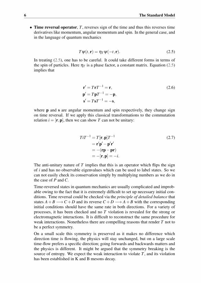
• Time reversal operator, T , reverses sign of the time and thus this reverses timederivatives like momentum, angular momentum and spin. In the general case, andin the language of quantum mechanics
T ψ(t,r) = ηT ψ(−t,r). (2.5)
In treating (2.5), one has to be careful. It could take different forms in terms ofthe spin of particles. Here ηT is a phase factor, a constant matrix. Equation (2.5)implies that
r′ = T rT−1 = r, (2.6)
p′ = T pT−1 =−p,s′ = T sT−1 =−s,
where p and s are angular momentum and spin respectively, they change signon time reversal. If we apply this classical transformations to the commutationrelation i = [r,p], then we can show T can not be unitary:
TiT−1 = T [r,p]T−1 (2.7)
= r′p′ −p′r′
=−(rp−pr)=−[r,p] =−i.
The anti-unitary nature of T implies that this is an operator which flips the signof i and has no observable eigenvalues which can be used to label states. So wecan not easily check its conservation simply by multiplying numbers as we do inthe case of P and C.
Time-reversed states in quantum mechanics are usually complicated and improb-able owing to the fact that it is extremely difficult to set up necessary initial con-ditions. Time reversal could be checked via the principle of detailed balance thatstates A+B −→C+D and its reverse C+D −→ A+B with the correspondinginitial conditions should have the same rate in both directions. For a variety ofprocesses, it has been checked and no T violation is revealed for the strong orelectromagnetic interactions. It is difficult to reconstruct the same procedure forweak interactions. Nonetheless there are compelling reasons that render T not tobe a perfect symmetry.
On a small scale this symmetry is preserved as it makes no difference whichdirection time is flowing, the physics will stay unchanged, but on a large scaletime-flow prefers a specific direction; going forwards and backwards matters andthe physics is different. It might be argued that the symmetry breaking is thesource of entropy. We expect the weak interaction to violate T , and its violationhas been established in K and B mesons decay.

2.2 Symmetry Properties 7
Let us have a brief look at the combined symmetries in the context of particlephysics.
CP symmetry: Within the standard SU(2)×U(1) electroweak model, with onlyone Higgs doublet, CP conservation is not exact. The CP violation is introduced viacomplex Yukawa couplings between the fermions and the Higgs boson. The Higgsboson acquires a vacuum expectation value through breaking the SU(2) symmetry andthen its interaction with quarks, Yukawa interaction, becomes mass mixing for quarks.The CP violation shows up in complex phases in the mixing matrices. By redefiningthe phase of various quark fields some of these phases could be removed. CP violationis ubiquitous in theories of new physics.
CPT symmetry: Each of P, C and T symmetries acting alone or even in a pairdo not leave a physical system invariant. The SM of particle physics predicts thatthe simultaneous application of all three transformations must be a symmetry. CPT isrequired to be conserved in any local quantum field theory.
From the CPT theorem one concludes that for any local hermitian Hamiltonian H,which is invariant under a proper Lorentz transformation that involves neither spacenor time inversions, there exists a choice of the phases, ηp,ηc and ηT , such that Hcommutes with the product of the operators P, C and T . CPT is basically the com-bined action of all three transformations that mandates particles and antiparticles musthave certain identical properties, such as the same mass, lifetime, charge and mag-netic moment. This is why we believe that if CP is violated in nature there must be acompensation to it to make CPT conserved, so T must also be violated.
Continuous space-time symmetries
In continuous groups the elements depend on one or more continuous parameters. Weare interested in internal symmetry transformations such as isospin, color and flavoursymmetries. These symmetries do not mix fields with different space-time properties.In other words, these transformations commute with the space-time components of thefields and therefore leave the Lagrangian invariant, but they can transform one parti-cle into another, rendering the same mass, but different quantum numbers. Continuoussymmetries have additive quantum numbers. There are two broad categories of discus-sion:
Global phase transformation: One of the internal degrees of freedom is codifiedin the form of a phase of the wave function. The Lagrangian of a reasonable theory isinvariant under a phase transformation of
ψ(x)−→Uψ(x)
U = eiα (2.8)
where α is a phase factor and it takes any real value. This phase transformation mightbe thought of as a multiplication of ψ by a unitary 1×1 matrix, group of U(1), and thesymmetry is called U(1) gauge invariance.
Local gauge transformation: The locally-symmetric theories enable us to derivethe physics. This class of symmetry transformations can be expressed as
ψ(x)−→ eiα(x)ψ(x). (2.9)

8 The Standard Model
Here the differentiable phase, α(x), has space-time dependency, it is a function of xμ ,
and in this sense is more general. The derivative of the transformation ∂μ(eiα(x)ψ(x))leads to new terms in the Lagrangian and to cancel them we have to introduce newfields and it turned out to be the case for the SM of particle physics.
The idea of local gauge invariance goes back to the work of Hermann Weyl in 1918[4]. The idea of locally symmetric transformations later in 1954 by Yang and Mills wasapplied to the group SU(2) and extended to SU(3) color symmetry [5].
2.3 Chiral Fermion State
The projection of the spin of the particle onto the direction of its momentum is calledhelicity
Helicity≡ S · P|P| . (2.10)
Since spin has a discrete value with regard to an axis, helicity is discrete as well. Forspin-half particles like fermions, if the helicity is positive, + h̄
2, it is called right-handed,otherwise the particle is left-handed. In other words, when the direction of momentumand spin of a particle are the same, it refers to right-handed, and vice versa. Mathe-matically, chirality is the sign of the projection of the spin vector onto the momentumvector, left is negative and right is positive. For massless spin-half particles, helicityis equivalent to the operator of chirality multiplied by 1
2. For massless particles forwhich helicity is frame independent, helicity and chirality are identical, on the contraryfor massive particles helicity is frame dependent and is not identical with chirality, sothere is no frame dependence of the weak interactions. Rotating the left-handed andright-handed components independently makes no difference on the theory, we say thatthe theory has chiral symmetry
{ψL −→ eiθLψLψR −→ ψR
, (2.11)
or {ψL −→ ψLψR −→ eiθRψR
. (2.12)
It can be seen that a mass term in the Lagrangian, mψ̄ψ breaks chiral symmetry, there-fore theories of massive fermions do not have chiral symmetry.
It appears that nature has a preference for left-handed fermions and they interactvia the weak interaction. In most circumstances, two fermions of left-handed chiralityinteract more strongly than right-handed or opposite-handed fermions, and it implies aviolation of the symmetry of the other forces of nature. Chirality does not respect the
parity symmetry either. By applying the projection operator, P± = 1±γ5
2 , on the Diracfield, a fermion would be reduced to its left or right-handed component:
ψL(x) =1
2(1− γ5)ψ(x),
ψR(x) =1
2(1+ γ5)ψ(x). (2.13)
2.4 Spontaneous Symmetry Breaking 9
Coupling of weak interactions to fermions is proportional to such a projection operator.The projection operator is responsible for parity symmetry violation. We must take intoaccount that, since γ5 is hermitian (γ5 = γ5†) it anticommutes with γμ
{γ5,γμ}= 0−→ γ5γμ =−γμγ5. (2.14)
Similarly for ψ̄(x) = ψ̄L(x)+ ψ̄R(x) we can consider
ψ̄L(x) = ψ̄(x)(1+ γ5)
2,
ψ̄R(x) = ψ̄(x)(1− γ5)
2. (2.15)
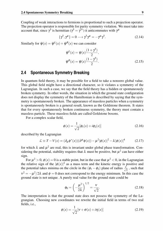
2.4 Spontaneous Symmetry Breaking
In quantum field theory, it may be possible for a field to take a nonzero global value.This global field might have a directional character, so it violates a symmetry of theLagrangian. In such a case, we say that the field theory has a hidden or spontaneouslybroken symmetry. In other words, the situation in which the ground state configurationdoes not display the symmetry of the Hamiltonian is described by saying that the sym-metry is spontaneously broken. The appearance of massless particles when a symmetryis spontaneously broken is a general result, known as the Goldstone theorem. It statesthat for every spontaneously broken continuous symmetry, the theory must contain amassless particle. These massless fields are called Goldstone bosons.
For a complex scalar field,
φ(x) =1√2[φ1(x)+ iφ2(x)] (2.16)
described by the Lagrangian
L≡ T −V (x) = (∂μφ ∗(x))(∂ μφ(x))−μ2|φ(x)|2−λ |φ(x)|4 (2.17)
for which λ and μ2 are real, this is invariant under global phase transformation. Con-sidering the potential, stability requires that λ must be positive, but μ2 can have eithersign.
For μ2 > 0, φ(x) = 0 is a stable point, but in the case that μ2 < 0, in the Lagrangianthe relative sign of the |φ(x)|2 as a mass term and the kinetic energy is positive andthe potential takes minima on the circle in the (φ1−φ2) plane of radius ν√
2, such that
ν2 =−μ2/2λ and φ = 0 does not correspond to the energy minimum. In this case theground state is not unique. A purely real value for the ground state could be
φ0 =
(−μ2
2λ
)1/2
=ν√2. (2.18)
The interpretation is that the ground state does not possess the symmetry of the La-grangian. Choosing new coordinates we rewrite the initial field in terms of two realfields, i.e.,
φ(x) =1√2[ν +σ(x)+ iη(x)] (2.19)

10 The Standard Model
where the term1√2[σ(x)+ iη(x)]
represents the quantum fluctuation about the minimum. Putting (2.19) back into (2.17)and expanding L about the vacuum in terms of the fields, we have
L′ = L0 +LI (2.20)
where
L0 =1
2(∂μσ(x))2 +
1
2(∂μη(x))2− 1
2[2λν2]σ2(x) (2.21)
and LI involves some constant, cubic and quartic interaction terms in σ(x) and η(x) inthe form of
LI =−λνσ(x)[σ2(x)+η2(x)]− 1
4λ [σ2(x)+η2(x)]2. (2.22)
It represents the interaction of the real fields with themselves.In principle, (2.17) and (2.20) are equivalent and a transformation of the type (2.19)
can not change the physics, but the L′ unlike the L gives the correct picture of physics inperturbation theory and one can calculate the fluctuation around the energy minimum.
The two first terms in L0 feature the kinetic energy of the fields and the third onehas the form of a mass term for the σ(x) field but there is no mass term associated withthe η(x) field, because mass arises from terms that are quadratic in the field. That is,the theory involves a massless scalar as well. This is known as a Goldstone boson andis due to being along the potential well, tangential direction, that is no restriction on it.This Lagrangian was only a simple example of a theory and involving several fields,one could get several Goldstone bosons.
If we consider the Lagrangian (2.17) for three interacting real fields φi(x) with i =1,2,3, in the case that μ2 < 0 and λ > 0, the new Lagrangian would describe a massivefield of mass (2λν2)1/2 and two massless Goldstone bosons [6].
2.5 The Higgs Mechanism
In the preceding discussion, we have seen that one of the ways the symmetry of aquantum field theory can be realized is a global symmetry, that is spontaneously broken,i.e., the vacuum state does not respect the symmetry and the particles do not formobvious symmetry multiplets. In such a theory for each generator of the spontaneouslybroken symmetry we have one massless scalar particle. Now we are going to considerlocal gauge symmetry in the theory. This leads to new possibilities. We will see thatspontaneous symmetry breaking causes a massless spin 1 gauge vector boson to acquiremass. The procedure of generating massive particles is known as “Higgs mechanism”.
In particle physics, the application of spontaneously broken local symmetry is in theweak interactions and this model unifies the weak interactions with electromagnetismin a single gauge theory.
Here it is considered that all of space is filled with the Higgs field. Part of the fieldmixes with the force carrying gauge fields to produce massive gauge bosons and therest describes Higgs bosons.

2.5 The Higgs Mechanism 11
These massive scalar bosons do not form a complete representation of the symme-try. This is the only way that vector particles like the W or Z can have mass. Thismechanism is an essential part of the SM.
When the symmetry of the Higgs field is spontaneously broken the gauge bosonparticles, such as W and Z particles get a mass as well as quarks and leptons. It can beinterpreted as a result of the interaction of the particles with the Higgs field.
As we saw for the Goldstone theorem, one of the fields was automatically massless.The spontaneous breaking of the local symmetry is accompanied by the appearance ofone or more massless, spin zero scalar particles4, Goldstone bosons, so our hope forfinding mass of the weak interaction gauge field, with the Goldstone mechanism, isshattered.
Taking a closer look, we can have an amazing twist in the story. It arises whenapplying the idea of spontaneous symmetry breaking to the case of local gauge invari-ance. The studied Lagrangian in the hidden sector can be rewritten if we consider, thistime, the combination of two real fields, φ1(x) and φ2(x), into a single complex field
φ(x) = φ1(x)+ iφ2(x), (2.23)
thus
|φ(x)|2 = φ ∗(x)φ(x) = φ 21 (x)+φ 2
2 (x). (2.24)
With this new notation the Lagrangian reads
L= (∂μφ)∗(∂ μφ)−μ2[φ ∗(x)φ(x)]−λ 2[φ ∗(x)φ(x)]2. (2.25)
Now the rotation symmetry, that was spontaneously broken, becomes an invarianceunder a U(1) global phase transformation
φ(x)−→ eiθ φ(x) (2.26)
where θ is any real number. For making the equation of motion invariant under localgauge transformations
φ(x)−→ eiθ(x)φ(x) (2.27)
by introducing a massless gauge field Aμ(x) and replacing ordinary derivatives by co-variant derivatives
∂μ −→ Dμ = ∂μ + iqAμ(x), (2.28)
the Lagrangian becomes
L= (Dμφ)∗(Dμφ)−μ2[φ ∗(x)φ(x)]−λ 2[φ ∗(x)φ(x)]2− 1
4Fμν(x)Fμν(x) (2.29)
where
Fμν(x) = ∂νAμ(x)−∂μAν(x) (2.30)
is the gauge invariant field strength tensor. This Lagrangian defines the Higgs modeland is invariant under a U(1) gauge transformation. Like the previous case we areinterested in studying the case that λ > 0 and μ2 < 0. Now we apply the same procedure
4The appearance of the zero mass bosons is a consequence of the degeneracy of the vacuum.

12 The Standard Model
as in section 2.4 to the locally invariant Lagrangian (2.29). We again obtain a circle ofminima in the φ1(x) and φ2(x) space that occur for
φ(x) = φ0 =
(−μ2
2λ
)1/2
eiθ , 0≤ θ ≤ 2π (2.31)
where θ describes a direction in the (φ1−φ2) plane. To apply the Feynman calculus,we have to expand the Lagrangian about a particular vacuum state. We take θ = 0 andfind
φ1min =
(−μ2
2λ
)1/2
=ν√2,
φ2min = 0. (2.32)
This choice is arbitrary and one can designate another value for θ . Defining new realfields, σ(x) and η(x) as before
σ(x) = φ1(x)− ν√2
η(x) = φ2(x) (2.33)
as fluctuations about this vacuum state, φ(x) becomes
φ(x) =1√2[ν +σ(x)+ iη(x)] (2.34)
Putting it back into the Lagrangian (2.29), we would have
L=1
2[(∂ μσ(x))(∂μσ(x))−λν2σ2(x)]+
1
2(∂μη(x))(∂ μη(x))
− 1
4Fμν(x)Fμν(x)+
1
2(qν)2Aμ(x)Aμ(x)+qνAμ(x)∂μη(x)
+ interaction terms+ constant (2.35)
The final constant is irrelevant and the interaction terms, which are cubic and quarticin the fields, specify various couplings of σ(x), η(x) and Aμ(x). The first line is the
same as before and describes a scalar particle, σ(x), of mass (2λν2)1/2 and a masslessGoldstone boson, η(x). The second line describes the free gauge field Aμ(x), but it hasacquired a mass.
Now, a question arises. Where does the mass of Aμ(x) come from? In the originalLagrangian, (2.29), we had a term of the form
φ ∗(x)φ(x)Aμ(x)Aμ(x) (2.36)
which would be present in the absence of spontaneous symmetry breaking (this cou-pling is depicted in left panel of figure 2.1), but when we consider fluctuation of theground state, the term presented by (2.36) takes the form of the Proca mass term. Thereis also the quantity in L
qνAμ(x)∂μη(x) (2.37)

2.5 The Higgs Mechanism 13
If we consider it as an interaction, it leads to a vertex of the form of figure 2.1 (rightpanel), in which the η(x) turns into an A(x). Such a bilinear in two different fieldsimplies that we have incorrectly identified the fundamental fields, or particles, in thetheory. Such an expression should be interpreted as an off-diagonal term in the massmatrix. The physical fields are those for which the mass matrix is diagonal. In otherwords, neither A(x) nor η(x) represents independent free particles. This difficulty isalso seen in comparing the number of degrees of freedom in the two physically identicalLagrangians (2.29) and (2.35).
φ(x)
φ(x)
Aμ(x)
Aμ(x) η(x) Aμ(x)
Figure 2.1: Coupling of four fields (left panel) and coupling of two independent fields (right
panel).
The problem can be resolved by using the local gauge invariance of (2.29) and theneliminating η(x) in (2.35). Rewriting equation (2.27) in terms of its real and imaginaryparts
φ(x)−→ φ ′(x) = eiθ(x)φ(x)= (cosθ(x)+ isinθ(x))(φ1(x)+ iφ2(x))= [φ1(x)cosθ(x)−φ2(x)sinθ(x)]+ i[φ1(x)sinθ(x)+φ2(x)cosθ(x)]= φ ′1(x)+ iφ ′2(x) (2.38)
and picking
θ =−arctan
(φ2(x)φ1(x)
), (2.39)
will render φ ′(x) real, which is equivalent to5
φ ′2(x) = η(x) = 0. (2.40)
In fact, a gauge transformation transforms φ(x) into a real field of the form
φ(x) =1√2[ν +σ(x)] (2.41)
In this particular gauge, called unitary gauge, in which the field has the form of (2.41),the Lagrangian reduces to
L= L0(x)+LI(x) (2.42)
5η(x) is called a ghost field.

14 The Standard Model
where
L0(x) =1
2[∂ μσ(x)][∂μσ(x)]− 1
2(2λν2)σ2(x)
− 1
4Fμν(x)Fμν(x)+
1
2(qν)2Aμ(x)Aμ(x). (2.43)
It involves only the quadratic terms and can be interpreted as the free Lagrangian den-sity of a real Klein-Gordon field σ(x) and a real massive vector field Aμ(x). There isno such term as (2.37) in it. And the interaction part is given by
LI(x) =−λvσ3(x)− 1
4λσ 4(x)+
1
2q2Aμ(x)Aμ(x)[2vσ(x)+σ2(x)]. (2.44)
On quantizing L0(x), σ(x) gives rise to neutral scalar bosons of mass (2λv2)1/2 andAμ(x) to neutral vector bosons of mass |qv|. In brief, by a choice of gauge, and consid-ering gauge invariance, we have eliminated the Goldstone boson and the offending termin the Lagrangian, and the degree of freedom of η(x) has been transferred to the mas-sive vector field Aμ(x). Now, the number of degrees of freedom in (2.29) and (2.35)that describe definitely the same physical system are equal. A massless vector fieldcarries two degrees of freedom, representing transverse polarizations, when Aμ(x) ac-quires mass, it picks up a third degree of freedom, longitudinal polarization. This extradegree of freedom comes from the Goldstone boson, which meanwhile by the Higgsmechanism disappeared from the theory. This phenomenon that a gauge field “eats”the Goldstone boson, and thereby acquires mass as well as a third polarization state,without disturbing the gauge invariance of the Lagrangian density is called the Higgsmechanism and the massive spin zero boson associated with the field σ(x) is called aHiggs boson [7, 8].
This was an example of application of the Higgs mechanism in the spontaneousbreaking of a U(1) local gauge symmetry. We can repeat the same procedure to thespontaneous breaking of local SU(2) symmetry. We see that we need at least one scalarSU(2) doublet, a Higgs doublet field, in order to break the symmetry spontaneously6.
2.6 The Electroweak Theory of Weinberg and Salam
In what follows we will get to know how spontaneous symmetry breaking, applying theHiggs mechanism, causes vector gauge bosons to acquire mass, but the photon remainsmassless. Basically the complete Lagrangian density of this model is described by
L= LL +LB +LH +LLH (2.45)
where LL refers to the leptonic part of the Lagrangian density7 and LB as a Lagrangiandensity for gauge bosons is
LB =−1
4Bμν(x)Bμν(x)− 1
4Giμν(x)G
μνi (x). (2.46)
6This happens in the SM. Nowadays there exist new ideas that consider two Higgs doublets, 2HDM [1].7It involves the left-handed fermion doublet and the right-handed fermion singlet.

2.6 The Electroweak Theory of Weinberg and Salam 15
Such a term describes gauge bosons in the absence of leptons and is invariant underSU(2)×U(1) gauge transformations. In equation (2.46), Bμν(x) and Gμν
i (x) are de-fined by
Bμν(x) = ∂ νBμ(x)−∂ μBν(x)
Gμνi (x) = Fμν
i (x)+gεi jkWμj (x)W
νk (x) (2.47)
withFμν
i (x) = ∂ νW μi (x)−∂ μW ν
i (x). (2.48)
Furthermore, LH denotes the Higgs part of the Lagrangian. According to this partvector gauge bosons become massive. It can be written as
LH = [DμΦ(x)]†[DμΦ(x)]−μ2Φ†(x)Φ(x)−λ [Φ†(x)Φ(x)]2 (2.49)
where in an arbitrary gauge Φ(x) is considered a doublet of four real scalar fields σ(x)and ηi(x), i = 1,2,3,
Φ(x) =1√2
(η1(x)+ iη2(x)
ν +σ(x)+ iη3(x)
). (2.50)
The covariant derivative DμΦ(x) is defined by
DμΦ(x) = [∂ μ + igτ jWμj (x)/2+ ig′Y Bμ(x)]Φ(x). (2.51)
Upon quantization, these fields lead to some difficulties, i.e., the SU(2)×U(1)gauge symmetry is spontaneously broken for the vacuum state in the case μ2 < 0 andλ > 0. We can get to the point that the appropriate vacuum expectation value for theHiggs field is
〈0|Φ(x)|0〉 ≡Φ0 =1√2
(0ν
)(2.52)
whereν =
(−μ2/λ)1/2
. (2.53)
Since Φ0 is neutral, the U(1)em symmetry with the choice IW = 12, IW
3 =−12 and Y = 1
2with generator
Y =Qe− IW
3 (2.54)
remains unbroken. i.e.,QΦ0 = 0. (2.55)
ThereforeΦ0 −→Φ′0 = eiα(x)QΦ0 = Φ0 (2.56)
where α(x) is an arbitrary function, so that the vacuum is invariant under U(1)em trans-formations and the photon remains massless. We mention that the vacuum does notrespect the SU(2)×U(1) symmetry. Here we again apply the Higgs mechanism, inanalogy with section 2.5 and then in the unitary gauge we pick up the form
Φ(x) =1√2
(0
v+σ(x)
)(2.57)

16 The Standard Model
for the isospinor scalar field about its ground state value. In the unitary gauge theηi(x) fields with i = 1,2,3 vanish. What is left is σ(x), that gives rise to the electricallyneutral, massive, spin zero Higgs scalar. Now putting (2.57) into the Lagrangian (2.45),we see that the electroweak vector bosons acquire mass, their masses are given as
mW =1
2vg mZ = mW/cosθW (2.58)
The masses predicted by the theory for mW and mZ are in good agreement with theexperimental values. For the neutral scalar Higgs particle we have
mH = (2λν2)1/2 (2.59)
The neutral Higgs particle is an eigenstate of charge-parity symmetry, CP, and consid-ered even. Great attention should be paid that the mass of the neutral Higgs boson isdetermined by considering only the first two terms of the potential
V(Φ(x)
)= μ2Φ†(x)Φ(x)+λ [Φ†(x)Φ(x)]2 + . . . . (2.60)
The value of the self-interaction constant, λ , can be determined from the Higgs mass,which now is known. Now we come to the last part of the complete Lagrangian, i.e.,LLH , which is defined by
LLH(x) =−gl[Ψ̄Ll (x)ψ
Rl (x)Φ(x)+Φ†(x)ψ̄R
l (x)ΨLl (x)]
−gνl [Ψ̄Ll (x)ψ
Rνl(x)Φ̃(x)+ Φ̃†(x)ψ̄R
νl(x)ΨL
l (x)] (2.61)
where gl and gνl are Yukawa coupling constants and the sum is over different types of
leptons. Φ(x) and Φ̃(x) are weak isospin doublets and defined by
Φ(x) =(
φa(x)φb(x)
),
Φ̃(x) =−i[Φ†(x)τ2]T =
(φ ∗b (x)−φ ∗a (x)
), (2.62)
where τ2 is the Pauli matrix and T denotes the transpose. The Lagrangian density(2.61) is invariant under SU(2)×U(1) gauge transformations. Doing some tediouscalculation lead us to the point that the first line of this Lagrangian, which obviouslyrepresents coupling of two leptons to one Higgs, yields
−glν√2[ψ̄L
l (x)ψRl (x)+ ψ̄R
l (x)ψLl (x)]+ · · · . (2.63)
It is equivalent to
−glν√2
ψ̄l(x)ψl(x). (2.64)
The term glν√2
refers to the lepton mass and the Yukawa coupling constant, gl , is pro-
portional to the lepton mass, ml . The theory could be easily extended to involve quarksand in the same manner one can see how quarks couple to the Higgs field and acquiremass due to invariance under SU(2)×U(1) gauge transformations. That is, the Higgscoupling to the fermions is proportional to their masses.
In this theory, which is well known as the “Standard Model”, the minimal choiceof a single Higgs doublet is sufficient to generate masses for gauge bosons, leptons aswell as quarks [7].

Chapter 3
Challenges for the Standard Model
3.1 Introduction
Why do we need to go beyond the SM?
The SM is a low-energy effective theory which happens to be renormalizable; hencehighly predictive, and it describes present collider data to a remarkable accuracy. Thegeneral question to ask is whether the Higgs mechanism as depicted in the SM is acomplete description of Electroweak Symmetry Breaking (EWSB) consistent with allexperimental data, or there is a more fundamental underlying dynamics that mimics aHiggs-like picture at the electroweak scale. On theoretical grounds, the latter seems tobe the case.
Even though no sign of new physics has been reported neither in electroweak pre-cision nor in flavour physics, the SM is not satisfactory and it is not believed to be theultimate theory. There is a list of unsolved problems in the physics of elementary par-ticles [9–11] and circumventing these problems provides a vast amount of motivationsfor new physics Beyond the Standard Model (BSM). For certain, some of those whichare most relevant to the work presented in this thesis will be emphasized below.
3.2 Baryon Asymmetry
It is evident that the idea of symmetry plays an important role in particle theory. Thissymmetry translates into the existence of a conservation law. To take an example,consider the electromagnetic interactions. Maxwell’s equations would still be validif we attempt to change all the positive charges into negative and vice versa. Thesymmetry ensures that the electric charge can not be created or destroyed and the netcharge of the Universe is expected to be zero.
The laws of physics also seem to fail to distinguish between matter and anti-matter.But we know that the Universe is mostly matter-dominated and especially baryons out-number anti-baryons. The baryon number, B, is a kind of charge which is attributed tothe baryons. In the same way, if one assigns -B as the baryon number for anti-baryons,the Universe must carry a net baryon number and one would speculate that B be a con-served quantity. Thus if B is non-zero presently, it could not be zero previously; hencebaryon asymmetry. In effect, annihilation between matter and antimatter has made thebaryon asymmetry much greater today than in the early Universe. Baryogenesis is the
18 Challenges for the Standard Model
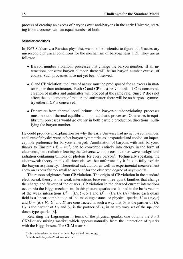
process of creating an excess of baryons over anti-baryons in the early Universe, start-ing from a cosmos with an equal number of both.
Sakharov conditions
In 1967 Sakharov, a Russian physicist, was the first scientist to figure out 3 necessarymicroscopic physical conditions for the mechanism of baryogenesis [12]. They are asfollows:
• Baryon number violation: processes that change the baryon number. If all in-teractions conserve baryon number, there will be no baryon number excess, ofcourse. Such processes have not yet been observed.
• C and CP violation: the laws of nature must be predisposed for an excess in mat-ter rather than antimatter. Both C and CP must be violated. If C is conserved,creation of matter and antimatter will proceed at the same rate. Since P does notaffect the total amount of matter and antimatter, there will be no baryon asymme-try either if CP is conserved.
• Departure from thermal equilibrium: the baryon-number-violating processesmust be out of thermal equilibrium, non-adiabatic processes. Otherwise, in equi-librium, processes would go evenly in both particle production directions, nulli-fying the baryon number.
He could produce an explanation for why the early Universe had no net baryon number,and laws of physics were in fact baryon symmetric, as it expanded and cooled, an imper-ceptible preference for baryons emerged. Annihilation of baryons with anti-baryons,thanks to Einstein’s E = mc2, can be converted entirely into energy in the form ofelectromagnetic radiation leaving the Universe with the cosmic microwave backgroundradiation containing billions of photons for every baryon1. Technically speaking, theelectroweak theory entails all three clauses, but unfortunately it fails to fully explainthe baryon asymmetry. Theoretical calculation as well as experimental measurementshow an excess far too small to account for the observed degree of asymmetry.
The reason originates from CP violation. The origin of CP violation in the standardelectroweak theory is the weak interactions between three quark families that changethe charge and flavour of the quarks. CP violation in the charged current interactionsoccurs via the Higgs mechanism. In this picture, quarks are defined in the basis vectorsof the weak interactions U ′ = (U1,U2,U3) and D′ = (D1,D2,D3) where each quarkfield is a linear combination of the mass eigenstates or physical quarks, U = (u,c, t)and D = (d,s,b). U ′ and D′ are constructed in such a way that U1 is the partner of D1,U2 is the partner of D2 and U3 is the partner of D3 in an arbitrary set of the up- anddown-type quarks [8].
Rewriting the Lagrangian in terms of the physical quarks, one obtains the 3× 3CKM quark mixing matrix2 which appears naturally from the interaction of quarkswith the Higgs boson. The CKM matrix is
1It is the interface between particle physics and cosmology.2Cabibbo-Kobayashi-Maskawa matrix.
3.3 Naturalness and Gauge Hierarchy Problem 19
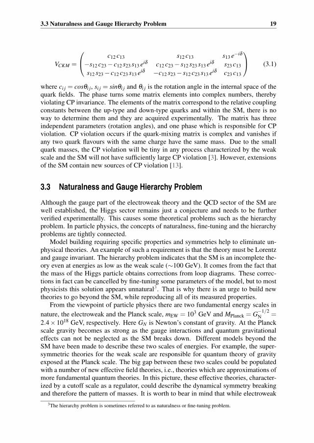
VCKM =
⎛⎝ c12 c13 s12 c13 s13 e−iδ
−s12 c23− c12 s23 s13 eiδ c12 c23− s12 s23 s13 eiδ s23 c13
s12 s23− c12 c23 s13 eiδ −c12 s23− s12 c23 s13 eiδ c23 c13
⎞⎠ (3.1)
where ci j = cosθi j, si j = sinθi j and θi j is the rotation angle in the internal space of thequark fields. The phase turns some matrix elements into complex numbers, therebyviolating CP invariance. The elements of the matrix correspond to the relative couplingconstants between the up-type and down-type quarks and within the SM, there is noway to determine them and they are acquired experimentally. The matrix has threeindependent parameters (rotation angles), and one phase which is responsible for CPviolation. CP violation occurs if the quark-mixing matrix is complex and vanishes ifany two quark flavours with the same charge have the same mass. Due to the smallquark masses, the CP violation will be tiny in any process characterized by the weakscale and the SM will not have sufficiently large CP violation [3]. However, extensionsof the SM contain new sources of CP violation [13].
3.3 Naturalness and Gauge Hierarchy Problem
Although the gauge part of the electroweak theory and the QCD sector of the SM arewell established, the Higgs sector remains just a conjecture and needs to be furtherverified experimentally. This causes some theoretical problems such as the hierarchyproblem. In particle physics, the concepts of naturalness, fine-tuning and the hierarchyproblems are tightly connected.
Model building requiring specific properties and symmetries help to eliminate un-physical theories. An example of such a requirement is that the theory must be Lorentzand gauge invariant. The hierarchy problem indicates that the SM is an incomplete the-ory even at energies as low as the weak scale (∼100 GeV). It comes from the fact thatthe mass of the Higgs particle obtains corrections from loop diagrams. These correc-tions in fact can be cancelled by fine-tuning some parameters of the model, but to mostphysicists this solution appears unnatural3. That is why there is an urge to build newtheories to go beyond the SM, while reproducing all of its measured properties.
From the viewpoint of particle physics there are two fundamental energy scales in
nature, the electroweak and the Planck scale, mEW = 103 GeV and MPlanck = G−1/2N =
2.4× 10¹⁸ GeV, respectively. Here GN is Newton’s constant of gravity. At the Planckscale gravity becomes as strong as the gauge interactions and quantum gravitationaleffects can not be neglected as the SM breaks down. Different models beyond theSM have been made to describe these two scales of energies. For example, the super-symmetric theories for the weak scale are responsible for quantum theory of gravityexposed at the Planck scale. The big gap between these two scales could be populatedwith a number of new effective field theories, i.e., theories which are approximations ofmore fundamental quantum theories. In this picture, these effective theories, character-ized by a cutoff scale as a regulator, could describe the dynamical symmetry breakingand therefore the pattern of masses. It is worth to bear in mind that while electroweak
3The hierarchy problem is sometimes referred to as naturalness or fine-tuning problem.

20 Challenges for the Standard Model
H H
H H H H
f
f̄φiφi
(a) (b) (c)
Figure 3.1: One loop radiative corrections to the Higgs squared mass parameter from a) quartic
Higgs self-coupling, b) gauge boson loops, c) heavy fermion loops f .
interactions have been probed at distances lEW = m−1EW, gravity has not yet been estab-
lished at distances as small as the Planck scale (LPlanck = M−1Planck). It is well-known that
the hierarchy problem has so huge a ratio of MPlanckmEW
.
The hierarchy problem occurs due to sensitivity of the scalar potential to newphysics. The electrically neutral part of the SM Higgs field is a complex scalar Hwith a potential described by (2.60)
V = μ2|Φ|2 +λ |Φ|4. (3.2)
It is known that the SM requires a non-vanishing VEV for φ at the minimum of thepotential. This will come through if λ > 0 and μ2 < 0 resulting in
〈Φ〉= ν =√−μ2/2λ (3.3)
which is approximately 246 GeV. The parameter v has the dimension of energy and setsthe scale of all masses in the theory, in principle. It can be concluded that m2
H is of theorder of (∼100 GeV)2. The discussion so far has been at tree level (no loops).
However, the problem is that when we calculate higher order corrections, the masssquared M2
H of the Higgs particle receives a quadratically divergent correction in theloop expansion from virtual effect of the SM particles that couple to the Higgs fieldin quantum field theory. If we assume the existence of a heavy scalar particle thatcouples to the Higgs boson, the Feynman diagrams in figures 3.1(a) and 3.1(b) willgive contributions and the Higgs boson mass squared will be sensitive to the mass ofthe heavy scalar particle [14].
If the Higgs field couples to a fermion, then the Feynman diagrams depicted infigure 3.1(c) introduce a correction4
δM2H ≈−|λ f |2 Λ2
UV (3.4)
where λ f is the Yukawa coupling proportional to gl and gνl (see Eq. (2.61)), and ΛUVis an ultraviolet momentum cutoff whose value should not be taken to infinity, insteadthe finite value of the cutoff corresponds to the energy scale at which the effect of thenew physics beyond the effective field theory becomes important. In other words, ΛUVis the energy scale at which new physics begins to change the behaviour of the theory.All SM fermions, leptons and quarks, can enter the loop. In case of the quarks the color
4The numerical factor is unimportant to our argument and harmlessly is omitted.

3.4 The Dark Matter Problem 21
factor is also involved, enhancing the contribution. The largest correction comes fromthe top quark with λ f ≈ 1.
The effect of such a contribution will be the modification of the bare mass term inthe potential (2.60) by the one-loop corrected physical value
M2physical ≈M2
0 −|λ f |2 Λ2UV . (3.5)
If the cutoff is of the order of the Planck scale then this quantum correction will beorders of magnitude larger than the required value of M2
H ∼ (100 GeV)2. Considering(3.5), with the assumption that ν is phenomenologically fixed, implies that the Higgscoupling λ f must be greater than unity. It follows that the Higgs sector will be stronglyinteracting, but it is unfavoured due to unitarity and perturbativity. The two-loop cor-rections involving a heavy fermion that couples indirectly with Higgs through gaugeinteractions could also affect the picture.
Such quadratic dependencies on the cutoff scale is present in theories with scalarfields. The quantum corrections to fermions and gauge bosons do not have direct sen-sitivity to the cutoff scale5, but since these particles acquire their masses via 〈φ〉 theentire mass spectrum of the SM is influenced by the cutoff ΛUV .
Three classes of solutions seem to be plausible to circumvent the problem:
• The problem would be much less severe if the new physics takes place at a scalesmaller than MPlanck, i.e., considering small value for the electroweak scale ΛUV[15]. Then one has to invent some new physics at the cutoff scale that alters prop-agation in the loop. It is not easy to accomplish it in a theory that possesses theLagrangian that solely accommodates two derivatives. Higher derivative theoriesusually fail either due to unitarity or causality [16].
• Introducing physics beyond the SM that contains partners to the SM particles:These new partner particles cancel off or control the quantum corrections, thequadratically divergent contributions to the Higgs scalar boson squared mass. Ex-amples include suppersymmetry and little Higgs theories [17, 18].
• Utilizing models in which the Higgs field is removed or emerges as a compos-ite bound state of fermions. Examples include technicolor and composite Higgsmodels [19].
In all these approaches, the existence of new particles are inevitable and may lead tonew signals at the LHC.
3.4 The Dark Matter Problem
Since introducing a dark matter candidate is a central ingredient to this work, moredetails will be presented in this section.
5The QED is regularized by the symmetry of gauge invariance (e.g. [20]).
22 Challenges for the Standard Model
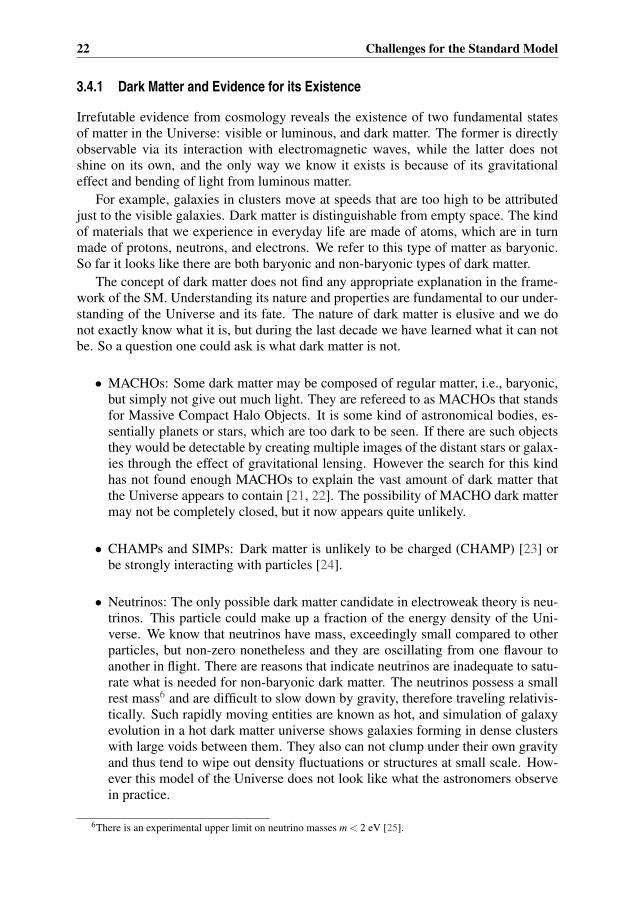
3.4.1 Dark Matter and Evidence for its Existence
Irrefutable evidence from cosmology reveals the existence of two fundamental statesof matter in the Universe: visible or luminous, and dark matter. The former is directlyobservable via its interaction with electromagnetic waves, while the latter does notshine on its own, and the only way we know it exists is because of its gravitationaleffect and bending of light from luminous matter.
For example, galaxies in clusters move at speeds that are too high to be attributedjust to the visible galaxies. Dark matter is distinguishable from empty space. The kindof materials that we experience in everyday life are made of atoms, which are in turnmade of protons, neutrons, and electrons. We refer to this type of matter as baryonic.So far it looks like there are both baryonic and non-baryonic types of dark matter.
The concept of dark matter does not find any appropriate explanation in the frame-work of the SM. Understanding its nature and properties are fundamental to our under-standing of the Universe and its fate. The nature of dark matter is elusive and we donot exactly know what it is, but during the last decade we have learned what it can notbe. So a question one could ask is what dark matter is not.
• MACHOs: Some dark matter may be composed of regular matter, i.e., baryonic,but simply not give out much light. They are refereed to as MACHOs that standsfor Massive Compact Halo Objects. It is some kind of astronomical bodies, es-sentially planets or stars, which are too dark to be seen. If there are such objectsthey would be detectable by creating multiple images of the distant stars or galax-ies through the effect of gravitational lensing. However the search for this kindhas not found enough MACHOs to explain the vast amount of dark matter thatthe Universe appears to contain [21, 22]. The possibility of MACHO dark mattermay not be completely closed, but it now appears quite unlikely.
• CHAMPs and SIMPs: Dark matter is unlikely to be charged (CHAMP) [23] orbe strongly interacting with particles [24].
• Neutrinos: The only possible dark matter candidate in electroweak theory is neu-trinos. This particle could make up a fraction of the energy density of the Uni-verse. We know that neutrinos have mass, exceedingly small compared to otherparticles, but non-zero nonetheless and they are oscillating from one flavour toanother in flight. There are reasons that indicate neutrinos are inadequate to satu-rate what is needed for non-baryonic dark matter. The neutrinos possess a smallrest mass6 and are difficult to slow down by gravity, therefore traveling relativis-tically. Such rapidly moving entities are known as hot, and simulation of galaxyevolution in a hot dark matter universe shows galaxies forming in dense clusterswith large voids between them. They also can not clump under their own gravityand thus tend to wipe out density fluctuations or structures at small scale. How-ever this model of the Universe does not look like what the astronomers observein practice.
6There is an experimental upper limit on neutrino masses m < 2 eV [25].

3.4 The Dark Matter Problem 23
3.4.2 WIMP Dark Matter and Favoured Candidates
Other non-baryonic dark matter may be tiny, sub-atomic particles which are not a partof normal matter at all. If these tiny particles have mass and if they are numerous andcold, they could make up a large part of the dark matter widely accepted to exist. Iftrue, then it is possible that most of the matter in the Universe is composed of somemysterious form yet to be identified. Today the main paradigm for the dark matter ofthe Universe has shifted to massive, non-relativistic and slowly moving particles whichare very weakly interacting, WIMPs.
The intriguing possibility is that this dark matter could consist of vast quantitiesof subatomic particles that do not interact electromagnetically, otherwise their electro-magnetic radiation would be detectable.
The evolution of galaxies would have been very different if the dark matter consistsof massive, slow-moving, and therefore cold particles. A problem is that there are nosuch entities known in the SM. This brings us to the ideas what lie beyond the SM.
Favoured candidates
Supersymmetry: The most prosperous theory postulates the existence of supersym-metric particles, the lightest of which, LSP, includes forms that do not respond to theelectromagnetic or strong forces, but they may be hundreds of times more massive thanthe proton. Once SU(2)×U(1) symmetry breaks, superpartners of the photon, Z, andneutral Higgs bosons, mix. Out of four such neutral states, neutralinos, the lightest oneis the most popular candidate for dark matter.
Extra dimensions: Some theorists suggest that our universe may have more spatialdimensions than what we are familiar with. General relativity was extended to five-dimensional space-time in an effort to unify gravity with the force of electromagnetism[26]; later it was postulated that the fifth dimension could be hidden by being curledup [27], for example, as if each point in our familiar space were actually a tiny ring(extra dimension) which a particle could run around. Particles moving through theextra dimensions could be massive owing to their extra-dimensional momentum and itscontribution to the rest mass.
In extra-dimensions theories, all the SM fields can propagate in one or more extradimensions. These are TeV-scale scenarios featuring the Kaluza-Klein excited statesof particles. These excited states of ordinary matter are known as KK modes and thelightest of them, the first KK excitation of the U(1)Y gauge boson, which is electricallyneutral and non-colored, is a suitable dark matter candidate.
Exotic candidates: In addition to the mainstream candidates above, many moreexotic candidates have been suggested such as WIMPzillas (with masses as large as1015GeV), Q-balls, gravitinos.
Scalar particles
Some extensions beyond the electroweak theory, while trying to explain some othershortcomings of the SM, provide a viable candidate for dark matter which, amongothers, meets the necessary requirements of the dark matter relic density. Like manyother models for dark matter, these models are equipped with some internal symmetries

24 Challenges for the Standard Model
to stabilize the dark matter over the age of the Universe. Two of these models are listedhere.
Little Higgs theories: The little Higgs theories, LH, are generally introduced toalleviate the Higgs hierarchy problem by putting forward a set of new particles. Con-tributions from new particles to the Higgs mass could eliminate the quadratic diver-gences at the one-loop level. With this mechanism, the LH models could stabilize theweak scale. They also give tree-level contributions to precision data. To constrain thisT -parity is applied to the model. Under this transformation, the SM particles stay unal-tered while all new particles become odd. In some varieties of the LH models known as"theory space”, the lightest T -odd particle is stable and could contribute to the matterdensity of cosmos.
Inert doublet models: It is assumed that the dark matter is made of a light spinlessparticle known as scalar dark matter, SDM. This candidate is predicted in differentextensions of the SM. They require the existence of a fundamental scalar field. Thesemodels intrinsically contain a spinless boson as a dark matter which is stable due to animposed Z2 symmetry.
Collisions at the large Hadron Collider at CERN may have enough energy to createthem. If such a particle is found, the challenge will then be to study its properties indetail, in particular to see if it could have formed large-scale clusters of dark matter inthe early Universe.
In this thesis the aim is to present two models that are trying to address some ofthese problems. In so doing, in the next chapter, we will study production and decayof the charged Higgs in the scope of type II 2HDM. Such a model is an extension tothe SM with a new spectrum of scalar particles. This introduces new sources of CPviolation and physics beyond the SM.
Next, in chapters 5 and 6, we will expand the particle content of the type II 2HDMwith a new scalar doublet. Such a model will inherit many features of the 2HDM. Thenew scalar doublet will not obtain any vacuum expectation value and by means of an adhoc Z2 symmetry its lightest neutral member will be stable enough to stand as a candi-date for the dark matter density of the Universe. The exploration of the viable parameterspace will be briefly presented. Then in chapter 6 decay and production mechanismsof the particles will be studied. Some selected regions of the parameter space will beconfronted with the latest data from direct and indirect detection experiments.

Chapter 4
Charged Higgs Production in type II 2HDM
4.1 Introduction
Albeit predictions of the SM are extremely well supported by the current data and themodel has been successfully confirmed by experimental precision tests, recent theoreti-cal and cosmological results demand its extension. Introducing only one Higgs doubletto break the symmetry in the SM is just an economical way, not the only possible one.There exists a number of motivation to extend the scalar sector of the SM [28–32]. Inprinciple, the presence of more doublets brings up many interesting phenomenologi-cal properties. After the discovery of the Higgs boson, the exploration of an extendedHiggs sector is of greater interest. In this connection, we focus our attention on theprospect of detecting the charged Higgs bosons at the LHC. We do it in the frameworkof the 2HDM with type II Yukawa couplings in which the Higgs sector is extended withan extra scalar doublet. In fact this chapter is an introduction to Paper I:
• Probing the charged Higgs boson at the LHC in the CP-violating type-II2HDM [34].
In the following, we will present the fields and the potential and then we will study thepossibility of detection of charged Higgs particles and identify a number of benchmarkpoints.
4.1.1 The Fields
The Higgs sector of the SM is augmented by a new doublet with the same quantumnumbers, namely weak isodoublets (T = 1/2) with hypercharge Y = 1. In fact, it buildsthe doublets of the 2HDM and they are expanded about their vacuum states as
Φi =
(ϕ+
i(νi +ηi + iχi)/
√2
), i = 1,2. (4.1)
Both doublets, in general, can acquire VEVs that break down the symmetry at treelevel. They can be written as
〈Φi〉=(
0
νi/√
2
), i = 1,2, (4.2)

26 Charged Higgs Production in type II 2HDM
whereν1 = ν cosβ , ν2 = ν sinβ , ν2 = ν2
1 +ν22 . (4.3)
The phases of Φ1 and Φ2 are chosen so that ν1 and ν2 are both real and non-negative.The parameter tanβ is the ratio of the two electroweak VEVs. We also define a massparameter μ , by μ2 = (v2/2v1v2)Re m2
12, and note that the following relation is estab-lished from the extremum condition:
Im m212 = ν1ν2Im λ5. (4.4)
With the introduction of two doublets, Φ1 and Φ2, we are exposed to the potentiallydangerous phenomenon of Flavour-Changing Neutral Current (FCNC) which experi-mentally is highly suppressed relative to the charged-current processes. To eliminatesuch an effect at tree level by Higgs mediated Yukawa couplings of the Lagrangian weimpose an appropriate discrete Z2 symmetry on the Lagrangian, potential and Yukawainteractions, in such a way that it is invariant when:{
Φ1 −→−Φ1
uR −→−uR(4.5)
with all other fields unchanged. The effect of the Z2 parity is to avoid Φ1 ←→ Φ2
transition [33].
4.1.2 The Potential and Parameters
The 2HDM can be classified according to its Higgs-fermion Yukawa interactions. Themodel we consider here is known as type-II [1] in which Φ1 couples to down-typequarks and charged leptons (I3 =−1/2) and Φ2 couples to up-type quarks (I3 = 1/2)1.The potential of the model reads:
V (Φ1,Φ2) =−1
2
{m2
11Φ†1Φ1 +m2
22Φ†2Φ2 +
[m2
12Φ†1Φ2 +h.c.
]}
+λ1
2(Φ†
1Φ1)2 +
λ2
2(Φ†
2Φ2)2 +λ3(Φ†
1Φ1)(Φ†2Φ2)
+λ4(Φ†1Φ2)(Φ†
2Φ1)+1
2
[λ5(Φ†
1Φ2)2 +h.c.
]. (4.6)
In order to allow for CP-violation in the scalar sector we allow for soft Z2 break-ing by adding the mass term m2
12Φ†1Φ2 + h.c. to the Z2-symmetric Lagrangian. The
parameter m12 is generally a complex parameter and m212 = 0.
The neutral states of Φ1,Φ2 will in general mix to form three neutral physical statesH1,H2,H3. These are linear combinations of η1, η2, and η3,⎛
⎝H1
H2
H3
⎞⎠= R
⎛⎝η1
η2
η3
⎞⎠ , (4.7)
where η3 ≡ −sinβ χ1 + cosβ χ2 and the rotation matrix R is parametrized in terms ofthree angles α1, α2 and α3 according to the convention of [72]. The model also containsa pair of charged scalar particles, H±. Therefore, eight distinct parameters can definethe parameter space of the model:
1Note that the 2HDM with type-II Yukawa interactions gives an effective description of the MSSM.

4.1 Introduction 27
M1, M2, MH± , μ , tanβ and αi with i = 1,2,3
From this input, the value of M3 and all λ ’s of the potential can be reconstructed [51].This multi-dimensional parameter space is constrained by a number of theoretical andexperimental conditions. To find the acceptable regions of the parameter space andthen select a set of benchmark points, the model is faced with all the theoretical andexperimental constraints in [34]. After the viable parameter space is found, we select anumber of benchmark points, shown in table 4.1, in two different scenarios:
• Low tanβ : with tanβ = 1, 2.
• High tanβ : with tanβ = 5,10.
The mass of the lightest neutral Higgs boson is taken to be M1 = 125 GeV and a rangeof charged Higgs boson masses is validated for fixed values of tanβ , μ and M2. Whentanβ is large (∼ 5− 10) the model gives rise to acceptable points only if MH± , μ andM2 are rather degenerate. Except P9 and P10 that fall close to a CP-conserving limit, theother benchmark points correspond to CP-violating scenarios.
α1/π α2/π α3/π tanβ μ M2 MminH± ,M
maxH±
P1 0.23 0.06 0.005 1 200 300 300,325
P2 0.35 −0.014 0.48 1 200 300 300,415
P3 0.35 −0.015 0.496 1 200 350 300,450
P4 0.35 −0.056 0.43 1 200 400 300,455
P5 0.33 −0.21 0.23 1 200 450 300,470
P6 0.27 −0.26 0.25 1 200 500 300,340
P7 0.39 −0.07 0.33 2 200 300 300,405
P8 0.34 −0.03 0.11 2 200 400 300,315
P9 0.47 −0.006 0.05 10 400 400 400,440
P10 0.49 −0.002 0.06 10 600 600 600,700
Table 4.1: Benchmark points selected from the allowed parameter space [34]. The mass pa-
rameter μ , the mass M2 and allowed range of MH± are in GeV.
4.1.3 BRs of Charged and Lightest Neutral Higgs Bosons
For the aforementioned benchmark points of the parameter space, the most relevantdecay modes for which BRs > 10−4 are determined. The branching ratios are displayedin figures 4.1 and 4.2. The results are presented for the range of MH± = 300−600 GeV.All of this range is not always inside the viable parameter space.
From figures 4.1 and 4.2, for two different values of tanβ , we can make a fewobservations:
• For the choice of tanβ = 1 the dominant decay mode is always tb and the branch-ing fraction for WH1 is about 0.1.

28 Charged Higgs Production in type II 2HDM
300 350 400 450 500 550 600
)±
BR
(H
-410
-310
-210
-110
1t b
1W H
t s
2W H
[GeV]±Hm
=1)β (tan1P
300 350 400 450 500 550 600)
±B
R (H
-410
-310
-210
-110
1t b
1W H
t s2W H 3W H
[GeV]±Hm
=1)β (tan2P
300 350 400 450 500 550 600
)±
BR
(H
-410
-310
-210
-110
1t b
1W H
t s2W H
3W H
[GeV]±Hm
=1)β (tan3P
300 350 400 450 500 550 600
)±
BR
(H
-410
-310
-210
-110
1t b
1W H
t s2W H 3W H
[GeV]±Hm
=1)β (tan4P
300 350 400 450 500 550 600
)±
BR
(H
-410
-310
-210
-110
1t b
1W H
t s2W H
[GeV]±Hm
=1)β (tan5P
300 350 400 450 500 550 600
)±
BR
(H
-410
-310
-210
-110
1t b
1W H
t s 2W H
[GeV]±Hm
=1)β (tan6P
Figure 4.1: Branching ratios of the charged Higgs versus mass for six benchmark with tanβ =1. Similar results were given in [34].

4.2 Charged Higgs Bosons at the LHC 29
• For the choice of tanβ = 2, when MH± ≥ 450 GeV, the decay channel H± →W±H2 becomes the dominant one, compared to H± → tb. It can be explained bythe fact that there is a suppression of the H± → tb coupling by a factor of about2 as well as a sizeable H± →W±H2 coupling.
• The τντ decay mode strongly depends on the tanβ value. For tanβ = 2 it reachesthe 10−3 level.
• For the case of tanβ = 2, the branching ratio for W±H1 depends quite a bit on thevalues of other parameters.
We are interested in the phenomenology of the charged Higgs boson produced inassociation with vector bosons. To understand the properties of the lightest neutralHiggs boson, we collect the relevant set of H1 branching ratios in table 4.2. We observethat the most important decay mode is always H1 → bb̄. Hence we will only considerthis decay channel for studying H1 signatures.
300 350 400 450 500 550 600
)±
BR
(H
-410
-310
-210
-110
1t b
1W H
t s
ντ
2W H 3W H
[GeV]±Hm
=2)β (tan7P
300 350 400 450 500 550 600
)±
BR
(H
-410
-310
-210
-110
1t b
1W H
t s
ντ
2W H 3W H
[GeV]±Hm
=2)β (tan8P
Figure 4.2: Branching ratios of the charged Higgs versus mass for two benchmark points.
Here, tanβ = 2. Similar results were given in [34].
4.2 Charged Higgs Bosons at the LHC
The production and detection mechanism for the charged Higgs vary in different massregions for the charged Higgs boson. For example, if MH± < mt −mb, the chargedHiggs will be mainly produced by gg→ tt̄ and qq̄→ tt̄ with subsequent decay of t →bH+ or t̄ → b̄H− [35]. In our study, we consider the single charged Higgs productionin association with the neutral Higgs, W bosons and quarks at the LHC for the centerof mass energies of
√s = 8 TeV and
√s = 14 TeV. The main partonic contributions to
these production channels are depicted in figure 4.3. They are as follows;
(gg,bb̄)→ H±W∓, (4.8)
qq̄′ → H±Hi, (4.9)
gg→ H+bt̄. (4.10)
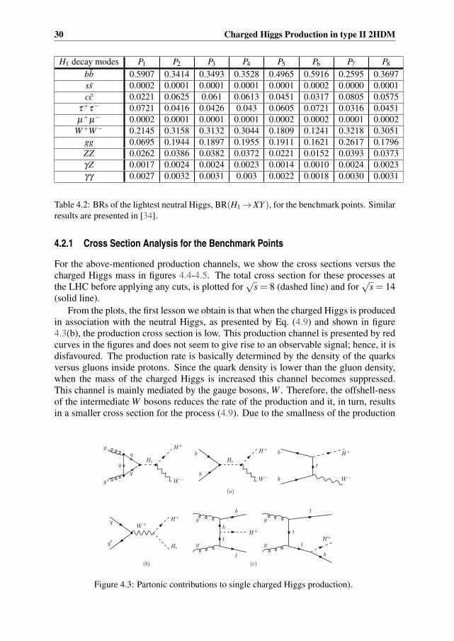
30 Charged Higgs Production in type II 2HDM
H1 decay modes P1 P2 P3 P4 P5 P6 P7 P8
bb̄ 0.5907 0.3414 0.3493 0.3528 0.4965 0.5916 0.2595 0.3697
ss̄ 0.0002 0.0001 0.0001 0.0001 0.0001 0.0002 0.0000 0.0001
cc̄ 0.0221 0.0625 0.061 0.0613 0.0451 0.0317 0.0805 0.0575
τ+τ− 0.0721 0.0416 0.0426 0.043 0.0605 0.0721 0.0316 0.0451
μ+μ− 0.0002 0.0001 0.0001 0.0001 0.0002 0.0002 0.0001 0.0002
W+W− 0.2145 0.3158 0.3132 0.3044 0.1809 0.1241 0.3218 0.3051
gg 0.0695 0.1944 0.1897 0.1955 0.1911 0.1621 0.2617 0.1796
ZZ 0.0262 0.0386 0.0382 0.0372 0.0221 0.0152 0.0393 0.0373
γZ 0.0017 0.0024 0.0024 0.0023 0.0014 0.0010 0.0024 0.0023
γγ 0.0027 0.0032 0.0031 0.003 0.0022 0.0018 0.0030 0.0031
Table 4.2: BRs of the lightest neutral Higgs, BR(H1→ XY ), for the benchmark points. Similar
results are presented in [34].
4.2.1 Cross Section Analysis for the Benchmark Points
For the above-mentioned production channels, we show the cross sections versus thecharged Higgs mass in figures 4.4-4.5. The total cross section for these processes atthe LHC before applying any cuts, is plotted for
√s = 8 (dashed line) and for
√s = 14
(solid line).
From the plots, the first lesson we obtain is that when the charged Higgs is producedin association with the neutral Higgs, as presented by Eq. (4.9) and shown in figure4.3(b), the production cross section is low. This production channel is presented by redcurves in the figures and does not seem to give rise to an observable signal; hence, it isdisfavoured. The production rate is basically determined by the density of the quarksversus gluons inside protons. Since the quark density is lower than the gluon density,when the mass of the charged Higgs is increased this channel becomes suppressed.This channel is mainly mediated by the gauge bosons, W . Therefore, the offshell-nessof the intermediate W bosons reduces the rate of the production and it, in turn, resultsin a smaller cross section for the process (4.9). Due to the smallness of the production
g
Hi
q
q
q
g
H+
W−
Hi
b
b
H+
W−
t
b
b
H+
W−
W+
q
q′
H+
Hi
g
g
H+
b
t̄
b
t
g
g
t
t̄
H+
b
t
(a)
(b) (c)
Figure 4.3: Partonic contributions to single charged Higgs production).

4.2 Charged Higgs Bosons at the LHC 31
cross section, this channel does not have any interesting phenomenological implicationat the LHC.
[GeV]+HM300 350 400 450 500 550 600
[fb]
σ
-110
1
10
210
310
W±Hi=1,2,3 H±H
t b±H8 GeV14 GeV
=1)β (tan1P
[GeV]+HM300 350 400 450 500 550 600
[fb]
σ
-110
1
10
210
310
W±Hi=1,2,3 H±H
t b±H8 GeV14 GeV
=1)β (tan2P
[GeV]+HM300 350 400 450 500 550 600
[fb]
σ
-110
1
10
210
310
W±Hi=1,2,3 H±H
t b±H8 GeV14 GeV
=1)β (tan3P
[GeV]+HM300 350 400 450 500 550 600
[fb]
σ
-110
1
10
210
310
W±Hi=1,2,3 H±H
t b±H8 GeV14 GeV
=1)β (tan4P
Figure 4.4: Production cross sections vs the charged Higgs mass for√
s = 8 (dashed line) and√s = 14 (solid line) for benchmark points 1−4. Similar results are presented in [34].
According to [1] the Yukawa couplings for the charged Higgs boson are expressedas
H+bt̄ :ig
2√
2mWVtb[mb(1+ γ5) tanβ +mt(1− γ5)cotβ ] (4.11)
H−tb̄ :ig
2√
2mWV ∗tb[mb(1− γ5) tanβ +mt(1+ γ5)cotβ ] (4.12)
and it shows that the associated production of the charged Higgs with quarks, Eq.(4.10), strongly depends on the value of tanβ . It also depends on the mass of thecharged Higgs, MH± . In fact, the dominant contribution in the coupling is proportionalto mt/ tanβ and the ratio of VEVs acts as a reduction factor when tanβ > 1. The Feyn-man diagram for this channel is shown in figure 4.3(c). The production cross sectionfor this channel is shown in brown in figures 4.4 and 4.5.
Let us look at associated production of a charged Higgs with a W boson, namelyEq. (4.8), the channel with a final H±W∓ state. This channel is mediated by the neutralHiggs. It is shown in figure 4.3, upper left.

32 Charged Higgs Production in type II 2HDM
[GeV]+HM300 350 400 450 500 550 600
[fb]
σ
-110
1
10
210
310
W±Hi=1,2,3 H±H
t b±H8 GeV14 GeV
=1)β (tan5P
[GeV]+HM300 350 400 450 500 550 600
[fb]
σ
-110
1
10
210
310
W±Hi=1,2,3 H±H
t b±H8 GeV14 GeV
=1)β (tan6P
[GeV]+HM300 350 400 450 500 550 600
[fb]
σ
-110
1
10
210
W±Hi=1,2,3 H±H
t b±H8 GeV14 GeV
=2)β (tan7P
[GeV]+HM300 350 400 450 500 550 600
[fb]
σ
-110
1
10
210
310
W±Hi=1,2,3 H±H
t b±H8 GeV14 GeV
=2)β (tan8P
Figure 4.5: Similar to figure 4.4, for benchmark points 5− 8. Similar results are presented
in [34].
The dominant production sub-processes, for the mass region selected here, are bb̄→H±W∓ at tree level and gg→ H±W∓ at one-loop level, depicted in 4.3(a). The lattercase results in a cross section that is enhanced for the choice of high M2 and M3 whenmW +MH± < Mi=2,3. The cross section for this channel is shown in blue in figures 4.4and 4.5.
In the allowed parameter space the corresponding cross sections show rather in-tricate behaviour. Figure 4.4 indicates that in the low-Higgs-mass scenario, whentanβ = 1 the cross section is competitive with the fermion-associated production.These qualitative conclusions also hold when tanβ is increased to 2, despite an overallsuppression due to the larger value of tanβ , involved in the H+bt̄ coupling in the formof mt/ tanβ .
The high-tanβ benchmark points, P9 and P10, give rather low production cross sec-tions that do not yield any useful signal after the cuts (discussed in 4.2.2) are applied.
4.2.2 Simulation of Signal and Background Events
In this section we would like to demonstrate the event analysis of the charged Higgsboson production in association with vector boson. Our preferred decay channel isH± →W±Hi. Proton-proton collision at the LHC produces the events of interest (sig-

4.2 Charged Higgs Bosons at the LHC 33
Generation cuts on background events
pTb > 20 GeV
|ηb|< 2.5∣∣M(bb)−120∣∣< 20 GeV
Table 4.3: Generation cuts.
nal) and a large number of background events. The aim is to introduce a number offilters to examine how the signal will look like after passing through the filtering lay-ers. We know that the charged scalar state does not belong to the particle spectrum ofthe SM. Hence the philosophy is that we presume the existence of new physics and tryto figure out how different will the signal be from the SM signal. The SM signals areusually dubbed as background events.
Generating events:The Monte Carlo-based (MC) data sample in our analysis, for both signal and back-
ground, was generated with the use of CalcHEP [66, 67]. It embraces all features of theprocess and provides a full description of the event. The generated events are in cor-respondence with an integrated luminosity of proton-proton collisions of 100 fb−1 andfor both signal and background, the same Parton Distribution Function, PDF, is used,namely CTEQ6.6M [36]. The neutral Higgs boson H1 decay branching ratio into a bb̄pair is about 80%, thus in the analysis we assume H1→ bb̄, hence the complete processfor the signal reads:
pp→W∓H± →W∓W±H1 →W∓W±bb̄. (4.13)
For this signal, the most important background at the LHC comes from top quark pairproduction which gives rise to the same kind of signature;
pp→ tt̄ →W∓W±bb̄. (4.14)
We consider the four-jet event topology for the signal. One jet pair originates fromhadronic W decay and the other W boson decays leptonically. Thus the signal event is:
pp→W∓H± →W∓W±H1 →W∓W±bb̄→ 2 j+2b+1�+MET. (4.15)
For each b or b̄ in the final state, in the process of event analysis a b-tagging efficiencyof ∼ 70% is assumed. For the W bosons, the full reconstruction efficiency is adopted.For event analysis for the signal 2 ·104 unweighted events are generated. These eventslead to a fairly nice reconstruction of the signal. For the top background, 4.5 · 106
unweighted events are produced. In the case of background events we have primarilyconsidered some cuts at the level of event generation, listed in table 4.3.
In reality experiments include uncertainty and each detector has its own energyresolution. In order to estimate the effects of a real LHC-prototype detector acceptanceand performance and emulate detector imperfections, we apply detector smearing toMC sample data. Therefore, the kinematic properties of of all visible final state particlesare modified. The smearing is done according to a Gaussian distributions with thedesign energy resolution of
a/√
E +b (4.16)

34 Charged Higgs Production in type II 2HDM
where E is measured in GeV. The parameters a and b stand for stochastic and constantterms, respectively. They are determined by test-beam experiments. For a jet (a,b) =(0.5,0.03) and for leptons (electrons and muons) (a,b) = (0.15,0.007) are considered.In fact, these values are for the ATLAS detector at LHC.
The event selection criteria:The study presented in the rest of this chapter is done differently from that of [34],
i.e., firstly, not the same Monte Carlo-based data sample is used and secondly, in theresults presented here we have utilized the program PYTHIA [69] and ROOT [70] inobtaining the results. That is why there are differences in what we present here withwhat was shown in [34]. The results are in a great agreement.
One of the most important problems in the analysis of high energy physics data isto discriminate new-physics signal against the SM background. In such an analysis, wewish to employ methods to optimize a figure of merit expressed as a function of signaland background, the signal-to-background significance (∼ S/
√B), in the signal region.
Significance is often used by physicists to express the cleanliness of the signal in thepresence of statistical fluctuations of observed signal and background [37]. To promotethe signal over background a decent set of filters is devised. We use the same selectioncuts for different mass regions and both on the signal and the background events asfollows:
• Standard kinematic cuts:These are usually standard detector acceptance cuts. In each event, leptons are requiredto have
pT� > 15 GeV, |η�|< 2.5, (4.17)
and the selected jets are required to have a jet-energy-scale-corrected
pTj > 20 GeV,
∣∣η j∣∣< 3, (4.18)
where pT and η are transverse momentum and pseudo-rapidity of the particle and aredefined as
pT =√
p2x + p2
y , (4.19)
η =1
2ln
( |p|+ pz
|p|+ pz
), (4.20)
with the z-axis defined as the incident proton beam direction. Here p is the particlemomentum. The condition on η is called the trigger acceptance. Cuts on pT and ηfeature a detector acceptance region.
The two jets and a jet and a lepton in (4.15) are required to be separated by at least
|ΔR( j, j)|> 0.5, |ΔR(�, j)|> 0.5, (4.21)
where ΔR =√
(Δη)2 +(Δφ)2 and Δφ(Δη) are differences in azimuthal scattering an-gle (pseudo-rapidity) between jets or/and a jet and a lepton. ΔR is the parameter ofseparation, thus small ΔR represents particles travelling in the same direction. This cutbasically has to do with detector resolution. If this criterion is not considered the twojets or a combination of a jet and a lepton will look like a single particle for the detector.This series of cuts can aid to reduce the QCD background.

4.2 Charged Higgs Bosons at the LHC 35
• Light Higgs reconstruction:
In order to attempt a Higgs mass reconstruction, with the assumption that the light SM-like Higgs boson mass is 125 GeV, a filter is applied on the invariant mass of the bb̄pair as follows: ∣∣M(bb)−125 GeV
∣∣< 20 GeV. (4.22)
• Hadronic W reconstruction (Wh → j j):
We demand that the final-state jets reconstruct the W boson and to do so event candi-dates must satisfy:
|M( j j)−80 GeV|< 20 GeV. (4.23)
• The top veto:
To reduce the backgrounds, this cut plays an important role. If ΔR(b1,Wh) <ΔR(b2,Wh), it is required that
M(b1 j j)> 200 GeV, (4.24)
andMT (b2�ν)> 200 GeV, (4.25)
otherwise 1↔ 2.
• The same-hemisphere b quarks:
Due to configuration of the signal and background, we employ another cut both onsignal and background events. For a good event, we have
pb1
|pb1| ·
pb2
|pb2| > 0 . (4.26)
In table 4.4, we show the efficiency of the previous set of cuts against the simulatedbackground for the P2, P4 and P5 points of table 4.1, for two values of charged Higgsmasses, namely MH± = 310 GeV and MH± = 390 GeV2. Similar results are also pre-sented in [34].
It is clearly demonstrated how the significance is influenced with imposing the cuts.There is a clear correlation between the MH± value and the efficiency of the top veto. Itis seen that the so-called “top veto" cut is the most effective cut of this set. The higherthe mass, the higher the efficiency. The results of table 4.4 are in good agreement withresults presented in [34]. From table 4.4, it is seen that further cuts are necessary toimprove the significance. In so doing, two more signal-based cuts are considered.
2For completeness, the conservative limit of MH± = 310 GeV is also shown, while a recent higher order
calculation of b→ sγ puts a limit on MH± in exclusion of values below ∼ 360−380 GeV [71].

36 Charged Higgs Production in type II 2HDM
Cut BG events BG Eff. (%) P2 events P2 Eff. (%) S/√
BKinematic 366566 100 72.5, 77.2 100, 100 0.1, 0.1
H1 reconstruction 327256 89.2 72.4, 77.1 99.9, 99.9 0.1, 0.1W reconstruction 321294 98.1 70.9, 75.7 98.0, 98.1 0.1, 0.1
top veto 2250 0.7 20.7, 37.9 29.3, 50.1 0.4, 0.8same-side b’s 872 38.8 18.9, 35.0 90.8, 92.2 0.6, 1.1
Cut BG events BG Eff. (%) P4 events P4 Eff. (%) S/√
BKinematic 366566 100 423.1, 213.0 100, 100 0.7, 0.3
H1 reconstruction 327256 89.2 422.9, 212.8 99.9, 99.9 0.7, 0.3W reconstruction 321294 98.1 414.1, 209.0 97.9, 98.2 0.7, 0.3
top veto 2250 0.7 51.2, 93.9 12.3, 44.9 1.0, 1.9same-side b’s 872 38.8 46.4, 87.5 90.5, 93.1 1.5, 2.9
Cut BG events BG Eff. (%) P5 events P5 Eff. (%) S/√
BKinematic 366566 100 1247.8, 484.4 100, 100 2.0, 0.8
H1 reconstruction 327256 89.2 1246.9, 483.8 99.9, 99.8 2.1, 0.8W reconstruction 321294 98.1 1214.5, 475.5 97.4, 98.2 2.1, 0.8
top veto 2250 0.7 133.7, 178.2 11.0, 37.47 2.8, 3.7same-side b’s 872 38.8 124.2, 164.7 92.8, 92.4 4.2, 5.5
Table 4.4: Consecutive efficiency of the cuts imposed on the top quark background and on the
benchmark points P2, P4 and P5 with MH± = 310 GeV and MH± = 390 GeV. The results are
consistent with [34].
• The signal-based selections:
The assumption is that the charged Higgs mass can be equivalently reconstructed byeither the invariant mass of the four jets (2b+2 j) or the transverse mass of the b jets, thelepton and the MET. For the signal, either of them will always reconstruct the correctcharged Higgs boson mass. It is indicated by a cross-like shape shown in figure 4.6, inwhich we adopt an illustrative choice of charged Higgs masses. Unlike the signal, thebackground events are piled up at ∼ 2mt . This feature motivates one to consider twomore filters in eliminating the top background:
Csqu = max(M(bb j j),MT (bb�ν)
)> Mlim (4.27)
andCsng = MT (bb�ν)> Mlim . (4.28)
We shall refer to Eq. (4.27) as squared cut and to Eq. (4.28) as single cut. The single cutof Eq. (4.28) is applied only on MT (bb�ν) because the reduction of the top backgroundis higher compared to a similar cut on the M(bb j j) for the same numerical value ofMlim.
The results for signal-to-background significance, after applying the cuts Csqu andCsng, are shown in tables 4.5, 4.6 and 4.7. Several values of Mlim for the points P2, P4
and P5 are considered and demonstrated.What emerges is that a higher value for Mlim results in an increase of the signifi-
cance by eliminating the top background more than the signal. It can be seen that Csqu
performs always better than the single cut.

4.2 Charged Higgs Bosons at the LHC 37
) [GeV]ν(bblTM100 200 300 400 500 600 700 800
M(b
bjj)
[GeV
]
100
200
300
400
500
600
700
800
Figure 4.6: M(bb j j) vs. MT (bb�ν) after cut 5 for (unweighed) point P5, with MH± = 310 GeV
(red) and MH± = 390 GeV (green). In blue is the (unweighed) top background. Similar figure
is presented in [34].
Cuttt P2 = 310 GeV P2 = 390 GeV
Events Events S/√
B Events S/√
B
Mlim = 450 GeVCsng 55.1 5.2 0.7 9.4 1.3Csqu 114.2 8.3 0.8 15.8 1.5
Mlim = 500 GeVCsng 38.6 4.9 0.8 8.5 1.4Csqu 82.5 7.9 0.8 14.6 1.6
Mlim = 550 GeVCsng 27.5 4.4 0.8 7.8 1.4Csqu 59.7 7.4 0.9 13.6 1.7
Mlim = 600 GeVCsng 19.6 4.0 1.0 7.0 1.6Csqu 42.3 6.8 1.0 12.7 1.9
Table 4.5: Comparison between Csqu and Csng vs Mlim for P2: surviving events and significance
with respect to the background. Similar results are also presented in [34].
• The peak cut:
By means of a new cut the evaluation of the significance can be limited to the peakregion. Such a cut is considered as:
|M−MH±|< 50 GeV, (4.29)
where M = min(M(bb j j),MT (bb�ν)
)when Eq. (4.27) is employed and M = M(bb j j)
when Eq. (4.28) is employed.For all benchmark points, the result for the significance analysis is collected in
table 4.8. In obtaining this table and in consistency with [34], the value Mlim = 600 GeVand the selection Csng are chosen. This choice seems to provide the best significance

38 Charged Higgs Production in type II 2HDM
Cuttt P4 = 310 GeV P4 = 390 GeV
Events Events S/√
B Events S/√
B
Mlim = 450 GeVCsng 55.1 10.2 1.3 22.9 3.0Csqu 114.2 17.0 1.6 39.27 3.6
Mlim = 500 GeVCsng 38.6 9.2 1.5 20.6 3.3Csqu 82.5 15.7 1.7 35.5 3.9
Mlim = 550 GeVCsng 27.5 8.3 1.6 18.8 3.6Csqu 59.7 14.5 1.8 32.2 4.1
Mlim = 600 GeVCsng 19.6 7.5 1.7 16.6 3.7Csqu 42.3 13.0 2.0 28.8 4.4
Table 4.6: Comparison between Csqu and Csng vs Mlim for P4: surviving events and significance
with respect to the background. Similar results are also presented in [34].
Cuttt P5 = 310 GeV P5 = 390 GeV
Events Events S/√
B Events S/√
B
Mlim = 450 GeVCsng 55.1 22.6 3.0 38.9 5.2Csqu 114.2 39.9 3.7 66.2 6.2
Mlim = 500 GeVCsng 38.6 20.2 3.2 35.7 5.7Csqu 82.5 34.0 3.7 60.4 6.6
Mlim = 550 GeVCsng 27.5 17.6 3.3 31.4 6.0Csqu 59.7 29.5 3.8 53.1 6.8
Mlim = 600 GeVCsng 19.6 14.5 3.2 27.8 6.3Csqu 42.3 24.9 3.8 47.3 7.2
Table 4.7: Comparison between Csqu and Csng vs Mlim for P5: surviving events and significance
with respect to the background. Similar results are also presented in [34].
while keeping a reasonable number of signal events for several of the benchmark points.The invariant mass distributions for some of the benchmark points are also plotted infigures 4.7–4.12. For each point, if possible, two values for the charged Higgs mass areconsidered, MH± = 310 GeV and MH± = 390 GeV.
At least three lessons emerge from the event study. They are the following:
• For P8, with tanβ = 2 and (MH2,MH±)= (400,310) GeV, no considerable number
of signal events is expected to survive after passing the filters.
• For P1, P2 (tanβ = 1, MH2= 300 GeV) and P7 (tanβ = 2, MH2
= 300 GeV) theproduction cross section is still large enough to give rise to observable signalswith respect to the background. From the plots, it is evident that for these bench-mark points the number of signal events is not above the background events.
• For P3, P4 and P5, for which tanβ = 1 and we have different allowed values forMH2
, when the mass of the charged Higgs is increased to higher allowed values(MH± = 390 GeV) the significance becomes larger and the signal would containa large number of events and its peak will always lie over the background.

4.2 Charged Higgs Bosons at the LHC 39
MH± = 310 GeV MH± = 390 GeV
Events S/√
B Events S/√
B
ttCsng 19.6
Csqu 42.3
Cpeak 4.7 − 6.3 −
P1
Csng 3.7 0.8 − −Csqu 7.2 1.1 − −Cpeak 3.5 1.6 − −
P2
Csng 4.0 0.9 7.1 1.6Csqu 6.8 1.0 12.7 1.9Cpeak 2.3 1.1 5.4 2.1
P3
Csng 8.8 2.0 18.2 4.1Csqu 15.4 2.4 30.2 4.7Cpeak 5.5 2.5 13.4 5.3
P4
Csng 7.5 1.7 16.6 3.7Csqu 13.0 2.0 28.8 4.5Cpeak 3.8 1.8 12.9 5.1
P5
Csng 14.5 3.2 27.8 6.2Csqu 24.9 3.9 47.3 7.2Cpeak 10.23 4.7 21.1 8.4
P6
Csng 13.1 2.9 − −Csqu 21.9 3.4 − −Cpeak 10.7 2.9 − −
P7
Csng 2.4 0.5 5.2 1.2Csqu 4.6 0.6 10.1 1.5Cpeak 2.0 0.9 4.7 1.8
P8
Csng 0 0 − −Csqu 1.5 0.3 − −Cpeak 0 0 − −
Table 4.8: Surviving events and their significance after the single cut of Eq. (4.28) and after
the peak selection of Eq. (4.29), for all points of table 4.1, except P9 and P10. Similar results
are also presented in [34].
The minor numerical differences between the results presented here and the resultsof [34] are due to the fact that different programs and events are used in extracting thenumerical results. Apparently, the Monte Carlo precision employed in the generationof the events as well as the process of smearing the events have influenced the results.

40 Charged Higgs Production in type II 2HDM
M(bbjj)[GeV]100 150 200 250 300 350 400 450 500 550 600
)-1Ev
ents
(L=1
00 fb
0
1
2
3
4
5 BG=310 GeV±HM
M(bbjj)[GeV]100 150 200 250 300 350 400 450 500 550 600
)-1Ev
ents
(L=1
00 fb
0
1
2
3
4
5 BG=310 GeV±HM
Figure 4.7: Points P1 (left panel) and P8 (right panel). Number of events integrated with
Lint = 100 fb−1 at√
s= 14 TeV vs M(bb j j) for signal (colored lines) and t-quark background.
M(bbjj)[GeV]100 150 200 250 300 350 400 450 500 550 600
)-1Ev
ents
(L=1
00 fb
0
1
2
3
4
5 BG=310 GeV±HM
M(bbjj)[GeV]100 150 200 250 300 350 400 450 500 550 600
)-1Ev
ents
(L=1
00 fb
0
1
2
3
4
5 BG=390 GeV±HM
Figure 4.8: Point P2. Similar to figure 4.7.
M(bbjj)[GeV]100 150 200 250 300 350 400 450 500 550 600
)-1Ev
ents
(L=1
00 fb
0
1
2
3
4
5 BG=310 GeV±HM
M(bbjj)[GeV]100 150 200 250 300 350 400 450 500 550 600
)-1Ev
ents
(L=1
00 fb
0
2
4
6
8
10BG
=390 GeV±HM
Figure 4.9: Point P3. Similar to figure 4.7.

4.2 Charged Higgs Bosons at the LHC 41
M(bbjj)[GeV]100 150 200 250 300 350 400 450 500 550 600
)-1Ev
ents
(L=1
00 fb
0
1
2
3
4
5 BG=310 GeV±HM
M(bbjj)[GeV]100 150 200 250 300 350 400 450 500 550 600
)-1Ev
ents
(L=1
00 fb
0
1
2
3
4
5
6
7
8
9 BG=390 GeV±HM
Figure 4.10: Point P4. Similar to figure 4.7.
M(bbjj)[GeV]100 150 200 250 300 350 400 450 500 550 600
)-1Ev
ents
(L=1
00 fb
0
2
4
6
8
10 BG=310 GeV±HM
M(bbjj)[GeV]100 150 200 250 300 350 400 450 500 550 600
)-1Ev
ents
(L=1
00 fb
0
2
4
6
8
10
12
14BG
=390 GeV±HM
Figure 4.11: Point P5. Similar to figure 4.7.
M(bbjj)[GeV]100 150 200 250 300 350 400 450 500 550 600
)-1Ev
ents
(L=1
00 fb
0
1
2
3
4
5 BG=310 GeV±HM
M(bbjj)[GeV]100 150 200 250 300 350 400 450 500 550 600
)-1Ev
ents
(L=1
00 fb
0
1
2
3
4
5 BG=390 GeV±HM
Figure 4.12: Point P7. Similar to figure 4.7.

42 Charged Higgs Production in type II 2HDM

Chapter 5
Two Higgs Doublets plus an Inert Doublet, theIDM2
5.1 Introduction
The scalar-sector structure of the SM contains only one doublet. The choice of onedoublet is only made for simplicity and several doublets could be included to explainthe breaking of the gauge symmetry via more complicated dynamics. On the one hand,we know that the tiny CP violation present in the SM can not account for the baryonasymmetry of the Universe. On the other hand, the mysterious nature of the dark matterthat comprises about 23% of the energy density of the Universe [38] is among thecompelling reasons to explore what might exist beyond the SM of particle physics.It seems that the introduction of new physics that provides more sources and a widerange of CP violation to explain the baryogenesis and at the same time accommodatesa dark matter candidate is a promising avenue. From this point of view, this chapter isdesignated to be an introduction to the second paper:
• Exploring the CP-Violating Inert-Doublet Model [39].
Here, we present a model that contains new sources of CP violation and at the sametime it introduces a new scalar particle as a dark matter candidate [39]. In this chapterthe goal is to present the model and to some extent discuss its viable parameter regionafter the discovery of the Higgs particle as well as the recent advances in dark matterdetection experiments. Further experimental aspects of the model will be discussed inchapter 6 as a review of [55].
5.2 Features of the Model
The model is one of the possible ways to embed the new physics within the oldparadigm to interpret the new observations. It is essentially an extension to the In-ert Doublet Model (IDM) [30, 38] which has been studied extensively in [32, 41–47].
We extend this model with the introduction of a new source of CP violation in thescalar sector by means of an extra doublet. Such a model accommodates some naturalfeatures. For example, it can make the electroweak phase transition fast [40]. Basicallythe resulting model could also be considered as an extension of the Two-Higgs-DoubletModel (2HDM) plus an inert doublet. The resulting model will be referred to as IDM2.

44 Two Higgs Doublets plus an Inert Doublet, the IDM2
5.2.1 The Fields
In the previous chapter, the Higgs sector of the type-II 2HDM was introduced. Nowwe extend this model with an inert doublet (dark doublet), for which the physical fieldappears as follows:
η =
(η+
(S+ iA)/√
2
). (5.1)
The dark doublet, η , transforms under an unbroken Z2 symmetry as
η Z2−→−η , (5.2)
which ensures the doublet is inert in the sense that η couples only bilinearly to otherscalars and the gauge sector. All other fields stay neutral under this transformation.The inert doublet possesses no vacuum expectation value, 〈η〉 = 0, implying that theZ2 symmetry associated with the inert doublet remains unbroken and therefore it doesnot participate in the Higgs mechanism. This feature ensures that the Z2 parity is notspontaneously broken by a vacuum expectation value and it stabilizes the lightest neu-tral inert particle to contribute to the dark matter density. Basically the scalar spectrumof the model is an extension to the particle content of the 2HDM with a pair of neu-tral inert particles, S and A, and a pair of charged states, η± (with physical massesMS,MA and Mη±)1. We assume that the scalar particle S is the lightest neutral one, i.e.,MS < MA; hence, the dark matter candidate.
5.2.2 The Potential
The potential of the model reads;
V (Φ1,Φ2,η) =V12(Φ1,Φ2)+V3(η)+V123(Φ1,Φ2,η), (5.3)
where V12(Φ1,Φ2) is the 2HDM potential, described by (4.6). The inert-sector potentialis
V3(η) = m2ηη†η +
λη
2(η†η)2. (5.4)
The mutual couplings of the inert and non-inert sectors are given by
V123(Φ1,Φ2,η) = λ1133(Φ†1Φ1)(η†η)+λ2233(Φ†
2Φ2)(η†η)
+λ1331(Φ†1η)(η†Φ1)+λ2332(Φ†
2η)(η†Φ2)
+1
2
[λ1313(Φ†
1η)2 +h.c.]+
1
2
[λ2323(Φ†
2η)2 +h.c.]. (5.5)
The parameters λ1133, λ2233, λ1331 and λ2332 are real, whereas λ1313 and λ2323 canbe complex. The CP is violated in the neutral non-inert scalar sector in the same wayas in the 2HDM [39].
1IDM2 bears some similarity to the three-Higgs-doublet Weinberg model [48, 49].

5.3 The Parameters of the Model 45
5.2.3 Dark Democracy
For the quartic couplings describing the interaction between η and Φ1 and Φ2, weadopt a simplifying assumption, the “dark democracy” [39]:
λa ≡ λ1133 = λ2233,
λb ≡ λ1331 = λ2332,
λc ≡ λ1313 = λ2323. (5.6)
Following (5.5), the parameters λa and λb are real. We furthermore assume that λc isreal. The physical masses of the dark sector are related to the parameters in the Higgspotential as
M2η± = m2
η +1
2λa ν2,
M2S = m2
η +1
2(λa +λb +λc)ν2,
M2A = m2
η +1
2(λa +λb−λc)ν2, (5.7)
where mη is a soft mass parameter of the inert sector potential (5.4), it has the dimen-sion of mass, but it is not the mass of any particle involved in the model. The softparameter indeed represents the bilinear couplings in the inert sector. From this pointof view, it will play an important role in determining the right amount of dark matterdensity; hence, the viable parameter space of the model. Inverting the relations (5.7)gives rise to
λa =2
ν2
(M2
η± −m2η
), (5.8a)
λb =1
ν2
(M2
S +M2A−2M2
η±), (5.8b)
λc =1
ν2
(M2
S −M2A). (5.8c)
The parameters λa, λb and λc represent couplings between non-inert and inert sectors.These parameters are related to mη . Thus, the couplings of the inert doublet to the non-inert Higgs sector can be expressed in terms of the mass splittings of the dark sectorparticles and the soft mass parameter mη . We also define
λL ≡ 1
2(λa +λb +λc) =
M2S −m2
η
ν2. (5.9)
5.3 The Parameters of the Model
The parameters of the Higgs potential are constrained by various theoretical conditionsas well as the observational constraints. These conditions are requirements for a phys-ically reasonable theory that are considered as a set of restrictions. Some of the theo-retical ones are absolute (for example, positivity), whereas the experimental ones are

46 Two Higgs Doublets plus an Inert Doublet, the IDM2
quantitative, and subject to experimental precision. A set of constraints are collected inPaper II [39].
The spectrum and the couplings are defined with the help of a total of 13 parameters.They are as follows:
- 2HDM sector: M1, M2, MH± , μ , tanβ and αi with i = 1,2,3.
- Inert sector: MS, MA, Mη± , λη and mη .
In order to determine allowed regions, some of these parameters are set to “inter-esting” values, adopted from prior studies. The rest of the parameters are scanned overin a hierarchical fashion, explained in [39]. The value of M3 and all λ ’s of the 2HDMpotential can be reconstructed by means of the 2HDM sector parameters [51]. The pa-rameters λa, λb and λc can also be determined using the inert-sector input. We scan overthe parameters and following [52, 53] focus on regions where the 2HDM is known tobe consistent. In general we employ different approaches for two different dark mattermass regions [39].
5.4 Allowed Parameter Domains
In this section we review some results of [39]. At the time this study was carried out themass of the Higgs boson was unknown and different values for M1 were contemplated.Among different values the case of M1 = 120 GeV was also studied. This was favoredby electroweak SM fits [54] and is very close to the mass of the Higgs boson that isnow known to be 125 GeV. That is the reason in the rest of this chapter we focus on thecases for which M1 = 120 GeV. We have found only two mass regions to give rise toconsistent solutions. In fact, the model is viable for medium (MS ∼ 75 GeV) and highmass regions (MS >∼ 550 GeV). In the following we review these two regions.
5.4.1 Medium Dark-Matter Mass Regime
For the medium range of dark-matter mass, some selected results are shown in fig-ure 5.1. In this figure the allowed regions are displayed in the Mη±–mη plane. Thevalues of M1 and MS are fixed, as indicated in the figures. Since the inert scalar particleS is assumed to be the dark matter candidate it is the lightest member of the inert sector,but there is no particular hierarchy between MA and Mη± . In fact, in cases presentedhere MA is fixed to 110 GeV adopted from [45].
An interesting feature for this mass domain is that the charged scalar from the darksector can acquire low mass without conflicting with any constraint. It arises from thefact that the inert doublet does not develop any vacuum expectation value, hence itsmembers have no Yukawa couplings, and are not affected by b→ sγ constraint on themass of charged particles contributing to this branching ratio.
In figures shown in this chapter2, the regions in blue demonstrate the viable param-eter space. In figure 5.1 the thin vertical solid lines indicate Mη± = MS and the dashedline at Mη± = 70 GeV gives the adopted experimental bound on the mass of the chargedscalar [50]. The default value of MA is also presented with a dashed line.
2The “holes” are presumably due to the small number of points being scanned over.
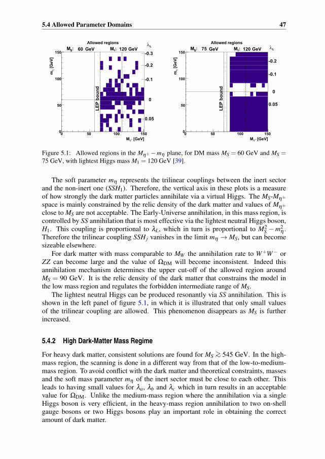
5.4 Allowed Parameter Domains 47
0 50 100 1500
50
100
150
0
-0.1
-0.2
-0.3
0.05
Allowed regions
[GeV
]η
m
[GeV]±ηM
:SM 60 GeV :1M 120 GeV
LEP
boun
d
Lλ
0 50 100 1500
50
100
150
0
-0.1
-0.2
0.05
Allowed regions
[GeV
]η
m
[GeV]±ηM
:SM 75 GeV :1M 120 GeV
LEP
boun
d
Lλ
Figure 5.1: Allowed regions in the Mη± −mη plane, for DM mass MS = 60 GeV and MS =75 GeV, with lightest Higgs mass M1 = 120 GeV [39].
The soft parameter mη represents the trilinear couplings between the inert sectorand the non-inert one (SSH1). Therefore, the vertical axis in these plots is a measureof how strongly the dark matter particles annihilate via a virtual Higgs. The MS-Mη±space is mainly constrained by the relic density of the dark matter and values of Mη±close to MS are not acceptable. The Early-Universe annihilation, in this mass region, iscontrolled by SS annihilation that is most effective via the lightest neutral Higgs boson,H1. This coupling is proportional to λL, which in turn is proportional to M2
S −m2η .
Therefore the trilinear coupling SSHj vanishes in the limit mη →MS, but can becomesizeable elsewhere.
For dark matter with mass comparable to MW the annihilation rate to W+W− orZZ can become large and the value of ΩDM will become inconsistent. Indeed thisannihilation mechanism determines the upper cut-off of the allowed region aroundMS = 90 GeV. It is the relic density of the dark matter that constrains the model inthe low mass region and regulates the forbidden intermediate range of MS.
The lightest neutral Higgs can be produced resonantly via SS annihilation. This isshown in the left panel of figure 5.1, in which it is illustrated that only small valuesof the trilinear coupling are allowed. This phenomenon disappears as MS is furtherincreased.
5.4.2 High Dark-Matter Mass Regime
For heavy dark matter, consistent solutions are found for MS >∼ 545 GeV. In the high-mass region, the scanning is done in a different way from that of the low-to-medium-mass region. To avoid conflict with the dark matter and theoretical constraints, massesand the soft mass parameter mη of the inert sector must be close to each other. Thisleads to having small values for λa, λb and λc which in turn results in an acceptablevalue for ΩDM. Unlike the medium-mass region where the annihilation via a singleHiggs boson is very efficient, in the heavy-mass region annihilation to two on-shellgauge bosons or two Higgs bosons play an important role in obtaining the correctamount of dark matter.

48 Two Higgs Doublets plus an Inert Doublet, the IDM2
Selected results on allowed regions in the Mη±–mη plane are displayed in figures 5.2and 5.3.
The other neutral and charged members of the inert doublet will also enter in theannihilation and coannihilation processes. They will be near-degenerate and severalchannels will be open. This will influence the way the viable parameter space is ob-tained in the lower and upper bounds of the heavy mass region by accommodating theobserved value of ΩDM [39].
550 552 554
546
548
550
552
554
0
-0.02
-0.04
-0.06
-0.08
0.02
0.04
0.06
0.08
Allowed regions
[GeV
]η
m
[GeV]±ηM
:SM 550 GeV :1M 120 GeV
AM
Lλ
800 805 810790
795
800
805
810
0
-0.05
-0.1
-0.15
-0.2
-0.25
0.05
0.1
0.15
0.2
0.25
Allowed regions
[GeV
]η
m
[GeV]±ηM
:SM 800 GeV :1M 120 GeV
AM
Lλ
Figure 5.2: Allowed regions in the Mη± −mη plane, for MS = 550 GeV, MA = 551 GeV (left
panel), and MS = 800 GeV, MA = 801 GeV (right panel) with M1 = 120 GeV. The thin solid
line indicates mη = MS, whereas the dashed line gives Mη± = MA [39].
In figure 5.3, allowed regions for dark-matter mass MS = 3000 GeV, MA =3001 GeV, and MS = 5000 GeV, MA = 5001 GeV are shown in the Mη± −mη plane.The solid line indicates mη = MS (λL = 0), whereas the dashed line gives Mη± = MA.The unitarity requirement plays an important role in constraining the parameter spacein the high mass region.
A complete set of figures and related results, concerning different mass domains ofthe dark matter, is presented in [39].

5.4 Allowed Parameter Domains 49
3000 3005 30102990
2995
3000
3005
3010
0 -0.1 -0.2 -0.3 -0.4 -0.5 -0.6 -0.7
0.1 0.2 0.3 0.4 0.5 0.6 0.7
Allowed regions
[GeV
]η
m
[GeV]±ηM
:SM 3000 GeV :1M 120 GeV
AM
Lλ
5000 5005 50104990
4995
5000
5005
5010
0
-0.2
-0.4
-0.6
-0.8
-1
-1.2
-1.4
0.2
0.4
0.6
0.8
1
1.2
1.4
Allowed regions
[GeV
]η
m
[GeV]±ηM
:SM 5000 GeV :1M 120 GeV
AM
Lλ
Figure 5.3: MS = 3000 GeV and 5000 GeV, both with M1 = 120 GeV [39].

50 Two Higgs Doublets plus an Inert Doublet, the IDM2

Chapter 6
Phenomenology and LHC Prospects of the IDM2
6.1 DM Identification
During the last decades, a notable experimental effort has been dedicated to identifyDM and unveil its nature. From the experimental point of view there are three possi-bilities to detect the DM candidate WIMP. The direct detection of the DM, the searchfor the DM particles scattering off the atomic nuclei, the indirect search for DM via itsannihilation to SM particles and the search for DM at particle colliders. This chapter ismostly adopted from:
• Exploring the CP-Violating Inert-Doublet Model [39].
• Phenomenology of charged scalars in the CP-Violating Inert-Doublet Model [55].
Here, we shall on one hand, confront the IDM2 with bounds from direct and indirectdetection experiments in the low-mass region and examine if the model is viable withrespect to experimental data. On the other hand, we aim to present the signals of theIDM2 and the way inert-sector particles can be produced and traced at colliders.
6.1.1 Direct Detection
The key assumption about the direct dark-matter detection experiments is that the darkmatter particles are WIMPs. In other words, they interact with ordinary matter via theweak force. The other assumption is that we have some idea of their mass and inter-action cross section. The interaction cross section of WIMPs with normal baryonicmatter is extremely small, but it is expected to have a non-zero value. This may enableus to detect and identify the nature of dark matter directly in a number of experimentsunder way. Although the sensitivity of dark matter detection has been continuously im-proved over the last years, until now all dedicated experiments have failed to report apositive signal1, but detectors using different materials and detection techniques havenot detected the dark matter particles. It seems there is still a long way to go, beforenon-detection would begin to rule out interesting WIMP candidates. Nowadays experi-ments are reaching the sensitivity to detect the most optimistic models for the WIMPs.
1Only the DAMA collaboration has reported seasonal variation in their detection rate [56–58]. DAMA does
not distinguish between WIMP signal and background on an event-by-event basis. Instead, the presence of
WIMPs may be inferred from the annual modulation in the rate of the lowest-energy single-scatter interactions,
assuming that the backgrounds do not modulate significantly [59].

52 Phenomenology and LHC Prospects of the IDM2
In this regard, we have chosen to confront our model with the recent CDMS-II [60] andXENON100 [61, 62] results for spin-independent scattering.
[GeV]SM10 210 310
]2[c
mσ
-4710
-4610
-4510
-4410
-4310
-4210
-4110WIMP- Nucleon Cross Sections
CDMS-II (2011)XENON100 (2011)XENON100 (2012)
Figure 6.1: Direct-detection WIMP-nucleon cross sections compared with the CDMS-II
(dashed) and XENON100 (solid) bounds.
In figure 6.1, we compare the direct-detection DM-nucleon cross sections for someof the acceptable model points with these recent constraints. These model points havepassed all the theoretical and experimental constraints discussed in [55] and are differ-ent from those of [39] in the sense that the recent LHC constraints are also consideredin obtaining them. For each studied value of MS, we show a “column” of cross sec-tion values corresponding to different values of the other parameters. The mass of thelightest neutral Higgs boson is taken to be M1 = 125 GeV. Values above the curvesare excluded by the CDMS-II (dashed curve) or the XENON100 (solid curve) exper-iments. It should be noted that the black solid curve represents the 2011 XENON100exclusion bounds [61], while the red curve represents the 2012 exclusion limits [62].Figure 6.1 reveals that around MS ∼ 60− 90 GeV, for a set of parameter points, thecross section of the dark matter particle can give a signal below the present upper lim-its on direct dark matter searches and much of the parameter space is compatible withthe current bounds. In the high DM-mass region, the predicted cross sections are verylow, implying that it would be difficult to test the model in the near future.
6.1.2 Indirect Detection
One of the indirect methods to detect dark matter is its subsequent annihilation, whichcould yield SM-particles like neutrinos or positrons that are potentially detectable, ordecay signal in gamma-rays. In the case of photons, electrically neutral dark matter an-nihilates via loop processes and produces monochromatic gamma-lines, either throughthe annihilation into two photons (γγ), a photon and a Z boson (γZ), or a photon and aHiggs boson(γH) [63].

6.2 Collider Signals 53
The Fermi-LAT collaboration has determined experimental upper bounds on al-lowed values for various annihilation cross sections multiplied by the velocity, 〈σv〉,based on various assumptions. These assumptions are referred to as “Conservative” as-sumptions, at 99.999% CL and 90% CL and “Stringent” exclusion [63]. In figure 6.2,we reproduce the exclusion bounds obtained for the annihilation cross section for
SS→ γγ (6.1)
according to both the conservative (upper two curves, solid lines) and the stringentapproaches. We find that 〈σv〉γγ depends on λ 2
L defined by Eq. (5.9) or in terms of thesplitting
〈σv〉γγ ∝ (M2S −m2
η)2 (6.2)
Here the conclusion is similar to the one for the direct-detection constraint. Infigure 6.2, the model expectations are shown in blue for M1 = 125 GeV and variousvalues of MS.
[GeV]SM10 210 310
/S]
3v[
cmσ
-2910
-2810
-2710
-2610
-2510
-2410
Fermi-LAT excluded
Allowed region
γγDM velocity-weighted annihilation cross section into
Figure 6.2: Fermi-LAT bounds on the velocity weighted annihilation cross section for SS→γγ .
6.2 Collider Signals
Due to the Z2 symmetry imposed on the potential, members of the inert doublet (η) canonly be produced in pairs at colliders
pp→ SSX ,AAX ,SAX ,Sη±X ,Aη±X ,η+η−X , (6.1)
with subsequent decay of A and η± to the lightest member, considered to be S. Inparticular, events with the charged scalars of the inert sector in the final state seem tobe very promising for the purpose of detection. Some of these processes, for directproduction, are shown in figure 6.3.

54 Phenomenology and LHC Prospects of the IDM2
η+
η−
γ/Z
q
q̄
η+
η−
Hi
q
q̄
g
Hi
q
q
q
g
η+
η−
W±
q
q̄′
η±
S
1
Figure 6.3: Direct production channels.
6.2.1 Charged Scalar Production at the LHC
In the following, we investigate the viability of producing charged scalar bosons at theLHC, by computing its production cross section for some representative benchmarkpoints in the parameter space. Some of these points, given in table 6.1, are takenfrom [55]. They fulfill all the theoretical and experimental requirements discussedin [55].
α1/π α2/π α3/π tanβ M2 M3 MH± R2HDMγγ RIDM2
γγ RIDM2γγ
P1 0.39 −0.026 0.46 1 300 333 400 0.92 0.50 0.34
P2 0.39 −0.009 0.025 1 300 325 400 0.91 0.50 0.34
P3 0.37 −0.018 0.016 1 300 394 400 0.78 0.45 0.30
P4 0.2 0.45 0.38 1 400 486 500 3.63 1.67 1.62
P5 0.19 0.46 0.39 1 400 501 500 4.02 1.84 1.8
P6 0.21 0.46 0.39 1 400 463 500 4.02 1.83 1.8
Table 6.1: Benchmark points selected from the allowed 2HDM parameter space. Some of
these points are taken from [55]. Masses are in GeV, μ = 200 GeV. Values of the ratio Rγγ are
given for the 2HDM, as well as for IDM2. Two values of Mη± are considered, 100 GeV and
200 GeV.
The search for the SM Higgs boson via the diphoton decay of the Higgs boson isperformed by the ATLAS and CMS collaborations [64, 65]. In Table 6.1 the value ofthis branching ratio, relative to that of the SM, has been presented,
Rγγ =Γ(H1 → gg)BR(H1 → γγ)
Γ(HSM → gg)BR(HSM → γγ). (6.2)
The ratio, Rγγ , is lowered by the contribution of the η± in the loop. For this study, wehave taken Mη± = 100 GeV (next-to-last column) and Mη± = 200 GeV (last column).
For comparison, its value in the absence of the η± contribution is also given.
In the following subsections, we study the production cross sections for η± in dif-ferent processes. These cross sections are computed by utilizing the code CalcHEP[66, 67].

6.2 Collider Signals 55
[GeV]±ηM100 120 140 160 180 200 220 240 260 280
[fb]
σ
10
210
310
S-η
S+η
[GeV]±ηM100 120 140 160 180 200 220 240 260 280
[fb]
σ
10
210
310
S ±η→ pp
Figure 6.4: Cross sections for η+S and η−S associated production at√
s = 14 TeV. Left:
Individual cross sections for η+S and η−S. Right: Sum. Similar results are shown in [55].
6.2.2 Associated production of η+S and η−S
The charged η± can be produced in association with the DM particle via an s-channelW -exchange. At the parton level we have:
qq̄′ →W±�→ η±S. (6.3)
The typical cross sections for this process are shown in figure 6.4 for P1 where theleft panel shows the η+ and η− produced separately via W+ and W−, respectively.Since there are more u quarks than d quarks in the protons, the rate for η+S productionwill be higher than that for η−S and therefore there will be more η+ produced thanη−. The summed cross section is shown in the right panel where the cross section is ofthe order of 100−1000 fb for Mη± up to a mass about 210 GeV.
6.2.3 Associated production of η+SX and η−SX :
A final state with a hard jet could be considered as well. In this case the cross sec-tion gets reduced. Typical cross sections are shown in figure 6.5 while these cuts areconsidered:
pminT = 20 GeV,
−4.5 < η(jet)< 4.5. (6.4)
The reasons for the interest in these signals are at least twofold. First the observationof events of this kind should be an instant evidence of new physics and second, it couldplay an important role in the search for scalar dark matter, i.e., the extra jet can help intriggering this kind of interaction.
6.2.4 Pair Production of Two Charged Particles, η+η−
The pair production mechanism at the parton level for η± can proceed as follows:
qq̄→ γ�,Z�→ η+η−, (6.5a)

56 Phenomenology and LHC Prospects of the IDM2
[GeV]±ηM100 120 140 160 180 200 220 240 260 280
[fb]
σ
10
210
310
S X+η S X-η
[GeV]±ηM100 120 140 160 180 200 220 240 260 280
[fb]
σ
10
210
310
S X±η→ pp
Figure 6.5: Cross sections for η+Sj and η−Sj associated production at√
s = 14 TeV. Left:
Individual cross sections for η+Sj and η−Sj. Right: Sum. Similar results are shown in [55].
gg→ H�i → η+η− i = 1,2,3. (6.5b)
For such processes the cross section is presented in figure 6.6, for the benchmarkpoints P3 and P5. The cross section depends on the soft parameter mη , for which twovalues are considered, representing two different strengths of the Hiη+η− coupling.The shoulders are obviously due to the cut-offs from contributions involving s-channelH2 and H3 exchange that correspond to 2Mη± = M2 and 2Mη± = M3, for various valuesof these masses. The cross section is of the order of 100− 500 fb, out to a mass Mη±of the order of 150 GeV.
The η± can decay to W±S. In a region of the parameter space the W± could beoff-shell and the virtual W± can decay leptonically. The lepton charge is of interest inthe detection of the new charged scalars and consequently the new physics.
[GeV]±ηM100 120 140 160 180 200 220 240 260 280
[fb]
σ
1
10
210
310-η+η→ pp
=20 GeVη m=80 GeVη m
)=(300, 394) GeV3, M2
(M
[GeV]±ηM100 120 140 160 180 200 220 240 260 280
[fb]
σ
1
10
210
310-η+η→ pp
=20 GeVη m=80 GeVη m
)=(400, 501) GeV3, M2
(M
Figure 6.6: Cross sections for η+η− pair production at√
s = 14 TeV. Left: P3, Right: P5.
Similar results are shown in [55].

6.2 Collider Signals 57
6.2.5 Decay of Charged scalars
In the region preferred by the DM, decays involving η± could lead to observable sig-nals. The combination of a small mass splitting between the charged scalar, η±, andthe inert one, S, can lead to long-lived charged scalars that decay away from the in-teraction point and give displaced vertices in LHC detectors. In the IDM2 when thedark matter is heavy, in order to have a consistent value for ΩDM a small mass split-ting is preferred for inert doublet members [39]. In the case of a light dark matter itis found that in a considerable part of the parameter space the mass splitting betweenη± and S could also be small [39]. In such a favourable situation, if charged scalarsare produced, they can decay to SW±. The W± then decays to fermions, as depictedin figure 6.7, that may enable η± to be detected [55]. Depending on the mass hierar-
η+(η) S(ps)
ν(q)
l+(p+)
W+(η − ps)
Figure 6.7: Decay of a charged scalar η+ to the DM particle S, a charged lepton and a neutrino.
chy between particles of the inert sector, also an A could be an intermediate state [68].Therefore the kinematically allowed decays, at the leading order, are
η± → S f f ′ (6.6)
η± → A f f ′. (6.7)
Thus, the η± width will be:
Γ = Γ(η± → SW±)+Γ(η± → AW±), (6.8)
where the W may be virtual. In figure 6.8, the branching ratios of η± (right panel) aswell as the decay width of the η± (left panel) is presented. The steep rise in the widthis when the W reaches threshold, at Mη± = MS +MW . The A would in turn decay,via a virtual or real Z to the S and two fermions. Such chains would thus yield fourfermions, occasionally three of which would be charged leptons. The S f f̄ ′ final statewould dominate when the S is significantly lighter than the A. The oscillations in theW±A branching ratio are due to WS reaching threshold for real W s, followed by WAreaching threshold for real W s.
6.2.6 Displacement of the Decay Vertex
It is found that in a significant fraction of the parameter space the mass splitting betweencomponents of the inert sector could be small. In such a condition longer life time isplausible for η± resulting in its decay away from the interaction point. As mentioned,

58 Phenomenology and LHC Prospects of the IDM2
[GeV]±ηM100 150 200 250 300 350 400
[GeV
]Γ
-510
-410
-310
-210
-110
1
10
decay width±η
[GeV]±ηM100 150 200 250 300 350 400
-410
-310
-210
-110
1 to A and S. ±ηBranching ratios of
S+ W→±η
A+ W→±η
Figure 6.8: Left: Decay width of the η±. Right: η± branching ratios to S or A, plus two
fermions [55].
the decay involves a virtual W , and the experimental signature in this case would bethe observation of an η± track from the production point up to its decay vertex in thedetector. This will be accompanied by a kink corresponding to the decay and a track ofthe charged lepton, if it decays leptonically or two jets if it decays hadronically. In thecase of leptonic decay such a kink does not depend on the nature of the accompanyingboson being produced; either η∓, A or S, at least one kink is always there. In each casesome missing energy through the presence of S’s in the final state will also be present.The displacement of the decay vertex depends on the mass splitting and the velocity ofη±.
[GeV]S-M±ηM0 0.5 1 1.5 2 2.5 3
m ]
μ [ λ
1
10
210
310
410
510
610
710A
M⟨SM
A M≈SM
Figure 6.9: Decay length λ vs. mass splitting Mη±–MS for two relative S–A spectra [55].
The decay length, λ = cτ , for η∓ is given in figure 6.9. If the η±-track falls into100 μm < λ < 1 m such a track, and the kink, could be seen in the detector. Theshaded region corresponds to this interval, which would be the experimentally interest-ing range. Note that the masses should differ by not more than 1 GeV for this to berelevant. The figure 6.9 is created for the rest frame of η±. In fact, the length of the dis-placement depends on the mass splitting of the inert members and the velocity of η±.

6.2 Collider Signals 59
For instance, if Mη± −MS = 0.3 GeV with the lifetime of τ = 1.23× 10⁻⁹ s and thevelocity of v = 0.9c, where c is the speed of light, the decay length would be L = 76.12cm. In other words, the decay length will be boosted by a factor of βγ where β = v/cand γ = 1/
√1−β 2.

60 Phenomenology and LHC Prospects of the IDM2

Chapter 7
Summary and conclusions
Our current description of the basic interactions in nature, based on the Standard Modelof particle physics, is in good agreement with all known experiments. However, it iscertainly fundamentally incomplete, as it does not provide enough CP violation andno candidate for the dark matter density of the Universe, among other things. Afterthe discovery of the Higgs boson, one important question is where to go beyond theStandard Model. The answer will of course depend on what is of most interest forphysics and what we are in search for!
One of the most promising ideas in theoretical particle physics is to consider morethan one doublet to break the symmetry of the gauge theory. Such an enriched modelwill be capable of addressing some shortcomings of the SM. The 2HDM and IDM2 fallinto such a class of theories.
In this thesis, we studied some features of these models. First, we considered the2HDM extension of the SM and studied production cross section for the charged Higgsboson in three different channels. We saw that if the charged Higgs bosons are pro-duced at the LHC, they will decay to SM particles. We considered a specific decaymode and performed an event study. A set of carefully devised filters could help us todistinguish the signals against the SM background. We showed the results for some se-lected regions of the parameter space and concluded that in most of them the signal liesabove the background.
Second, the IDM2 was introduced and its viable parameter space was explored. Themodel was required to satisfy the observed dark matter relic density, among all othertheoretical and experimental conditions. The model is valid in two different regions forthe dark matter mass. The members of the inert doublet can be pair-produced at theLHC. In some region of the parameter space, when the masses of these particles areclose to each other, the charged member can decay away from the interaction point.
The decay products could be leptons and missing energy or two jets and missingenergy. Depending on the mass of the charged scalar and the phase space, the two jetscould be treated as two separate jets or an effective mono-jet.
It might leave some signals enabling these particles to be detected.

62 Summary and conclusions

Bibliography
[1] J. F. Gunion, H. E. Haber, G. L. Kane and S. Dawson, Front. Phys. 80, 1 (2000).1, 6, 4.1.2, 4.2.1
[2] A. Djouadi, Phys. Rept. 457, 1 (2008) [arXiv:hep-ph/0503172]. 1
[3] M. B. Gavela, P. Hernandez, J. Orloff and O. Pene, Mod. Phys. Lett. A 9, 795(1994) [arXiv:hep-ph/9312215]. 1, 3.2
[4] H. Weyl, Sitzungsber. Preuss. Akad. Wiss. Berlin (Math. Phys. ) 1918, 465 (1918).2.2
[5] C. -N. Yang and R. L. Mills, Phys. Rev. 96, 191 (1954). 2.2
[6] F. Halzen and A. D. Martin, New York, USA: Wiley ( 1984) 396p 2.4
[7] F. Mandl and G. Shaw, Chichester, UK: Wiley (2010) 478 p. 2.5, 2.6
[8] M. E. Peskin and D. V. Schroeder, Reading, USA: Addison-Wesley (1995) 842 p2.5, 3.2
[9] S. Troitsky, Phys. Usp. 55, 72 (2012) [Usp. Fiz. Nauk 182, 77 (2012)][arXiv:1112.4515 [hep-ph]]. 3.1
[10] K. Nakamura et al. [Particle Data Group Collaboration], J. Phys. G 37, 075021(2010). 3.1
[11] A. Pomarol, CERN Yellow Report CERN-2012-001, 115-151 [arXiv:1202.1391[hep-ph]]. 3.1
[12] A. D. Sakharov, Pisma Zh. Eksp. Teor. Fiz. 5, 32 (1967) [JETP Lett. 5, 24 (1967SOPUA,34,392-393.1991 UFNAA,161,61-64.1991)]. 3.2
[13] Y. Grossman, Y. Nir and R. Rattazzi, Adv. Ser. Direct. High Energy Phys. 15, 755(1998) [arXiv:hep-ph/9701231]; Y. Nir, [arXiv:hep-ph/9911321]. 3.2
[14] A. Djouadi, Phys. Rept. 459, 1 (2008) [hep-ph/0503173]. 3.3
[15] C. Csaki, arXiv:hep-ph/0404096. 3.3
[16] D.A. Eliezer and R.P. Woodard, Nucl. Phys. B 325, 389 (1989). 3.3
[17] S. P. Martin, arXiv:hep-ph/9709356. 3.3

64 BIBLIOGRAPHY
[18] M. Perelstein, Prog. Part. Nucl. Phys. 58, 247 (2007) [arXiv:hep-ph/0512128].3.3
[19] For reviews, C. T. Hill and E. H. Simmons, Phys. Rept. 381, 235 (2003)[Erratum-ibid. 390, 553 (2004)] [arXiv:hep-ph/0203079]; K. D. Lane, arXiv:hep-ph/9401324; K. Lane, arXiv:hep-ph/0202255. 3.3
[20] I. J. R. Aitchison and A. J. G. Hey, Bristol, UK: IOP (2003) 406 p 5
[21] P. Tisserand et al. [EROS-2 Collaboration], arXiv:astro-ph/0607207. 3.4.1
[22] C. Alcock et al. [MACHO Collaboration], arXiv:astro-ph/9803082. 3.4.1
[23] S. Dimopoulos, D. Eichler, R. Esmailzadeh and G. D. Starkman, Phys. Rev. D 41,2388 (1990). 3.4.1
[24] G. D. Starkman, A. Gould, R. Esmailzadeh and S. Dimopoulos, Phys. Rev. D 41,3594 (1990). 3.4.1
[25] W. M. Yao et al. [Particle Data Group], J. Phys. G 33, 1 (2006). 6
[26] O. Klein, Z. Phys. 37, 895 (1926) [Surveys High Energ. Phys. 5, 241 (1986)].3.4.2
[27] L. Randall and R. Sundrum, Phys. Rev. Lett. 83, 4690 (1999) [hep-th/9906064].3.4.2
[28] R. S. Gupta and J. D. Wells, Phys. Rev. D 81 (2010) 055012. 4.1
[29] F. J. Botella, G. C. Branco and M. N. Rebelo, Phys. Lett. B 687 (2010) 194. 4.1
[30] R. Barbieri, L. J. Hall and V. S. Rychkov, Phys. Rev. D 74 (2006) 015007[arXiv:hep-ph/0603188]. 4.1, 5.2
[31] E. Ma, Phys. Rev. D 73 (2006) 077301 [arXiv:hep-ph/0601225]. 4.1
[32] Q. H. Cao, E. Ma and G. Rajasekaran, Phys. Rev. D 76 (2007) 095011[arXiv:0708.2939 [hep-ph]]. 4.1, 5.2
[33] S. L. Glashow and S. Weinberg, Phys. Rev. D 15, 1958 (1977). 4.1.1
[34] L. Basso, A. Lipniacka, F. Mahmoudi, S. Moretti, P. Osland, G. M. Pruna andM. Purmohammadi, arXiv:1205.6569 [hep-ph]. (document), 4.1, 4.1.2, 4.1, 4.1,4.2, 4.2, 4.4, 4.5, 4.2.2, 4.2.2, 4.4, 4.6, 4.5, 4.2.2, 4.6, 4.7, 4.8, 4.2.2
[35] Z. Kunszt and F. Zwirner, Nucl. Phys. B385, 3 (1992), and references citedtherein. 4.2
[36] P. M. Nadolsky et al., Phys. Rev. D78, 013004 (2008), arXiv:0802.0007. 4.2.2
[37] I. Narsky, physics/0507157. 4.2.2
[38] N. G. Deshpande and E. Ma, Phys. Rev. D 18, 2574 (1978). 5.1, 5.2

BIBLIOGRAPHY 65
[39] B. Grzadkowski, O. M. Ogreid and P. Osland, Phys. Rev. D 80 (2009) 055013[arXiv:0904.2173 [hep-ph]]. (document), 5.1, 5.2.2, 5.2.3, 5.3, 5.4, 5.1, 5.4.2,5.2, 5.4.2, 5.3, 6.1, 6.1.1, 6.2.5
[40] L. Fromme, S. J. Huber and M. Seniuch, JHEP 0611, 038 (2006) [hep-ph/0605242]. 5.2
[41] M. Cirelli, N. Fornengo and A. Strumia, Nucl. Phys. B 753, 178 (2006)[arXiv:hep-ph/0512090]. 5.2
[42] L. Lopez Honorez, E. Nezri, J. F. Oliver and M. H. G. Tytgat, JCAP 0702, 028(2007) [arXiv:hep-ph/0612275]. 5.2
[43] T. Hambye and M. H. G. Tytgat, Phys. Lett. B 659, 651 (2008) [arXiv:0707.0633[hep-ph]]. 5.2
[44] S. Andreas, T. Hambye and M. H. G. Tytgat, JCAP 0810, 034 (2008)[arXiv:0808.0255 [hep-ph]]. 5.2
[45] E. Lundstrom, M. Gustafsson and J. Edsjo, Phys. Rev. D 79, 035013 (2009)[arXiv:0810.3924 [hep-ph]]. 5.2, 5.4.1
[46] T. Hambye, F. S. Ling, L. Lopez Honorez and J. Rocher, JHEP 0907, 090 (2009)[arXiv:0903.4010 [hep-ph]]. 5.2
[47] L. Lopez-Honorez and C. E. Yaguna, JCAP 1101, 002 (2011). [arXiv:1011.1411[hep-ph]]. 5.2
[48] S. Weinberg, Phys. Rev. Lett. 37, 657 (1976). 1
[49] G. C. Branco, Phys. Rev. D 22, 2901 (1980). 1
[50] A. Pierce and J. Thaler, JHEP 0708, 026 (2007) [arXiv:hep-ph/0703056]. 5.4.1
[51] W. Khater and P. Osland, Nucl. Phys. B 661 (2003) 209 [arXiv:hep-ph/0302004].4.1.2, 5.3
[52] A. W. El Kaffas, P. Osland and O. M. Ogreid, Phys. Rev. D 76, 095001 (2007)[arXiv:0706.2997 [hep-ph]]. 5.3
[53] A. W. El Kaffas, O. M. Ogreid and P. Osland, [arXiv:0709.4203 [hep-ph]]. 5.3
[54] C. Amsler et al. [Particle Data Group], Phys. Lett. B 667, 1 (2008).
[55] P. Osland, A. Pukhov, G. M. Pruna and M. Purmohammadi, JHEP 1304 (2013)040 [arXiv:1302.3713 [hep-ph]]. 5.4(document), 5.1, 6.1, 6.1.1, 6.2.1, 6.1, 6.4, 6.5, 6.6, 6.2.5, 6.8, 6.9
[56] R. Bernabei et al. [DAMA Collaboration], INFN-AE-98-23. R. Bernabei, P. Belli,F. Cappella, R. Cerulli, F. Montecchia, F. Nozzoli, A. Incicchitti and D. Prosperiet al., Int. J. Mod. Phys. D 13, 2127 (2004) [astro-ph/0501412]. 1

66 BIBLIOGRAPHY
[57] R. Bernabei, P. Belli, F. Montecchia, F. Nozzoli, F. Cappella, A. Incicchitti,D. Prosperi and R. Cerulli et al., 1
[58] R. Bernabei, P. Belli, F. Montecchia, F. Nozzoli, F. Cappella, A. d’Angelo, A. In-cicchitti and D. Prosperi et al., Int. J. Mod. Phys. Conf. Ser. 12, 37 (2012). 1
[59] R. W. Schnee, arXiv:1101.5205 [astro-ph.CO]. 1
[60] Z. Ahmed et al. [ The CDMS-II Collaboration ], Science 327, 1619-1621 (2010).[arXiv:0912.3592 [astro-ph.CO]]. 6.1.1
[61] E. Aprile et al. [ XENON100 Collaboration ], Phys. Rev. Lett. 107, 131302(2011). [arXiv:1104.2549 [astro-ph.CO]]. 6.1.1, 6.1.1
[62] L. S. Lavina [ for the XENON100 Collaboration], arXiv:1305.0224 [hep-ex].6.1.1, 6.1.1
[63] A. A. Abdo et al. [Fermi-LAT Collaboration], JCAP 1004, 014 (2010)[arXiv:1002.4415 [astro-ph.CO]]. 6.1.2
[64] G. Aad et al. [ATLAS Collaboration], Phys. Lett. B 716, 1 (2012)[arXiv:1207.7214 [hep-ex]]. 6.2.1
[65] S. Chatrchyan et al. [CMS Collaboration], Phys. Lett. B 716, 30 (2012)[arXiv:1207.7235 [hep-ex]]. 6.2.1
[66] A. Pukhov, (2004), arXiv:hep-ph/0412191. 4.2.2, 6.2.1
[67] A. Belyaev, N. D. Christensen and A. Pukhov, Comput. Phys. Commun. 184, 1729(2013) [arXiv:1207.6082 [hep-ph]]. 4.2.2, 6.2.1
[68] B. Grzadkowski, O. M. Ogreid, P. Osland, A. Pukhov, M. Purmohammadi, JHEP1106, 003 (2011). [arXiv:1012.4680 [hep-ph]]. 6.2.5
[69] T. Sjostrand, S. Mrenna and P. Z. Skands, JHEP 0605, 026 (2006) [hep-ph/0603175]. 4.2.2
[70] R. Brun, F. Rademakers and S. Panacek, “ROOT, an object oriented data analysisframework,”; R. Brun and F. Rademakers, Nucl. Instrum. Meth. A 389, 81 (1997).4.2.2
[71] T. Hermann, M. Misiak and M. Steinhauser, JHEP 1211, 036 (2012)[arXiv:1208.2788 [hep-ph]]. 2
[72] E. Accomando et al., arXiv:hep-ph/0608079. 4.1.2

Scientific results

68 Scientific results