Embed Size (px)
Citation preview

An Explicit Mapped Tent Pitching Scheme forMaxwell Equations
Jay Gopalakrishnan, Matthias Hochsteger, Joachim Schoberl, and ChristophWintersteiger
Abstract We present a new numerical method for solving time dependent Maxwellequations, which is also suitable for general linear hyperbolic equations. It is basedon an unstructured partitioning of the spacetime domain into tent-shaped regionsthat respect causality. Provided that an approximate solution is available at the tentbottom, the equation can be locally evolved up to the top of the tent. By mappingtents to a domain which is a tensor product of a spatial domain with a time in-terval, it is possible to construct a fully explicit scheme that advances the solutionthrough unstructured meshes. This work highlights a difficulty that arises when stan-dard explicit Runge Kutta schemes are used in this context and proposes an alter-native structure-aware Taylor time-stepping technique. Thus explicit methods areconstructed that allow variable time steps and local refinements without compro-mising high order accuracy in space and time. These Mapped Tent Pitching (MTP)schemes lead to highly parallel algorithms, which utilize modern computer archi-tectures extremely well.
1 Introduction
Electromagnetic waves propagate at the speed of light. Thus, the field at a certainpoint in space and time depends only on field values within a dependency cone.A tent pitching method introduces a special “causal” spacetime mesh that respectsthis finite speed of propagation. It is not limited to Maxwell equations, but can be
Jay GopalakrishnanFariborz Maseeh Department of Mathematics & Statistics, Portland State University, PO Box 751,Portland OR 97207-0751, USA, e-mail: [email protected]
Matthias Hochsteger, Joachim Schoberl, Christoph WintersteigerInstitute for Analysis and Scientific Computing, Technische Universitat Wien, Wied-ner Hauptstraße 8-10, 1040 Wien, Austria, e-mail: [email protected],[email protected], [email protected]
1

2 J. Gopalakrishnan, M. Hochsteger, J. Schoberl, C. Wintersteiger
applied to general hyperbolic equations. A tent pitching method requires a numer-ical scheme to discretize the equation on that mesh. Discontinuous Galerkin (DG)methods are of particular interest since they offer a systematic avenue to build highorder methods. For a given initial condition at the bottom of a tent, the discrete equa-tions may be solved within each individual tent, up to the tent top. The computedsolution at the tent top provides initial conditions for the tents that follow later intime. This method is highly parallel, since many tents can be solved independently.Methods using such tent-pitched meshes may be traced back to [5, 7]. More recentworks [1, 6, 8] develop Spacetime DG (SDG) methods within tents by formulatinglocal variational problems, for which linear systems are set up and solved. Althoughthese systems are local, the matrix size can grow rapidly with the polynomial order,especially in four-dimensional spacetime tents. In this context it is natural to ask ifone can develop explicit schemes (which usually perform well under low memorybandwidth) that take advantage of tents.
A key ingredient to answer this question was presented in [2], where MappedTent Pitching (MTP) schemes were introduced. The MTP discretization, which pro-ceeds by mapping tents to a spacetime cylinder, allows one to evolve the solutioneither implicitly or explicitly within tents. The memory requirements of the explicitMTP scheme are limited to what is needed for storing the spatial mesh, the solutioncoefficients at one time step, and the topology of the tents.
In this work, we show that notwithstanding the above-mentioned advantages ofthe explicit MTP scheme, one may lose higher order convergence if a naive timestepping strategy (involving a standard explicit Runge-Kutta scheme) is used. Wethen develop a new Taylor time-stepping for the local problems within tents. De-spite its simplicity, our numerical experiments show that it delivers optimal order ofconvergence.
2 Mesh generation by tent pitching
We start with a conforming spatial mesh consisting of elements T = {T} and ver-tices V = {V}. We progress in time by defining a sequence of advancing fronts τi.A front τi is given as a standard nodal finite element function on this mesh. It isdefined by storing the current time for every vertex of the mesh. We move from τito the next front τi+1 by moving one vertex forward in time, while keeping all othervertices fixed. The spacetime domain between τi and τi+1 we call a tent. In Fig. 1,the red domain is the tent between τi and τi+1.
Its projection to the spatial domain is exactly the vertex patch ωV around V ofthe original mesh. The data to be stored for one tent are the bottom and top-times ofthe central vertex, plus the times for all neighboring vertices.
Note that although the algorithm is described sequentially, it is highly parallel.Vertices with graph-distance of at least two can be moved forward independently.For example, in Fig. 1, all blue tents can be built and processed in parallel.

MTP scheme for Maxwell Equations 3
The distance for advancing a vertex is limited by the speed of light, a constraintoften referred to in the literature as the causality condition. Under this condition, theMaxwell problem inside the tent is solvable using the initial conditions at the tentbottom. Thus, the top boundary is an outgoing boundary and no boundary conditionsare needed there.
Note that the spatial mesh is refined towards the right boundary, which leadsto smaller tent heights at the right boundary. Hence, smaller time steps in locallyrefined regions is a very natural feature of tent pitching methods.
τi
x
t
Fig. 1 Tent pitched spacetime mesh for a one-dimensional spatial mesh.
3 The MTP discretization
Now, we consider the discretization method for one tent domain K = {(x, t) : x ∈ωV ,ϕb(x) ≤ t ≤ ϕt(x))}, where ωV is the union of elements containing the vertexV , and ϕb and ϕt are the bottom and top fronts, respectively, restricted to ωV . Ouraim is to numerically solve the Maxwell system on K, namely
∂tεE = ∇×H , ∂t µH =−∇×E , (1)
where boundary values for both fields are given at the tent bottom and ∇ = ∇xdenotes the spatial gradient.
The approach of MTP schemes is to map the tent domain to a spacetime cylinderωV × (0,1) and solve the transformed equation there. The transformation from thecylinder to the tent is denoted by Φ : ωV × (0,1)→ K and is defined by Φ(x, t) =(x,ϕ(x, t)) where
ϕ(x, t) = (1− t)ϕb(x)+ tϕt(x) .
It is similar to the Duffy transformation mapping a square to a triangle.With the notation
skewE =
0 Ez −Ey−Ez 0 ExEy −Ex 0
,
we can rephrase the curl operator as ∇× E = divskewE, where the divergenceof the matrix function is taken row-wise. To simplify notation further, we defineu : K→ R6 by u = (E,H), and set g : K→ R6 and f : K→ R6×3 by

4 J. Gopalakrishnan, M. Hochsteger, J. Schoberl, C. Wintersteiger
ωV
K
x
t
ωV
K = ωV × (0,1)
x
tΦ
Fig. 2 Tent mapped from a tensor product domain.
g(u) =[
εEµH
], f (u) =
[−skewH
skewE
]. (2)
Then (1) may be rewritten as the conservation law ∂tg(u)+divx f (u) = 0. Further-more, we define F(u) ∈ R6×4 as
F(u) = [ f (u) g(u)] =[−skewH εE
skewE µH
],
which allows us to write Maxwell’s system (1) as the spacetime conservation law
divx,t F(u) = 0 . (3)
For each row of F , the spacetime divergence divx,t sums the spatial divergence ofthe first three components with the time-derivative of the last component.
Now, we apply the Piola transformation to pull back F from the tent K to thecylinder using the mapping Φ . The derivative of Φ and its transposed inverse are
Φ′ =
[I 0
∇ϕT δ
]and (Φ ′)−T =
[I −δ−1 ∇ϕ
0 δ−1
].
The Piola transform of F is F(u) =P{F}= (detΦ ′)(F ◦Φ)(Φ ′)−T with u= u◦Φ .Since the Piola transform provides an algebraic transformation of the divergence,equation (3) is simply transformed to divx,t F(u) = 0 on the spacetime cylinder.Then, inserting the Jacobian of Φ leads us to the transformed equation
∂t(g(u)− f (u)∇ϕ)+divx(δ f (u)) = 0 , (4)
where δ (x) = ϕt(x)−ϕb(x) is the local height of the tent. Note that ∇ϕ is an affine-linear function in quasi-time t. Equation (4) describes the evolution of u along quasi-time from t = 0 to t = 1. Details of the calculations are given in [2].
The next step is the space discretization of (4) by a standard discontinuousGalerkin method. Let Vh ⊂ [L2]
6 be the DG finite element space of degree p on T .On each tent we search for u : [0,1]→Vh such that∫
ωV
∂t[g(u)− f (u)∇ϕ
]vh− ∑
T⊂ωV
∫T
δ f (u)∇vh + ∑F⊂ωV
∫F
δ fn(u+, u−)JvK = 0

MTP scheme for Maxwell Equations 5
holds for all vh ∈ Vh and all t ∈ [0,1]. Only the restriction of Vh on the patch ωV isused in this equation. The numerical flux fn(u+, u−) depends on the positive tracelims→0+ u(x+ sn) and negative trace lims→0+ u(x− sn), where n is a unit normalvector of arbitrary orientation to the face. The jump is defined as usual by JuK :=u+− u− and the mean value by {u} := 1
2 (u+ + u−). One example is the upwind
flux [3, p. 434]
fn(u+, u−) =[{H}×n+ JEtK−{E}×n+ JHtK
],
with the tangential components Et = −(E×n)×n and Ht = −(H×n)×n of E =E ◦Φ and H = H ◦Φ . Note that the local tent height δ enters the boundary integralsas a multiplicative factor. At the outer boundary of the vertex patch we have δ = 0,so the facet integrals on the outer boundary disappear. For the above semidiscretesystem, initial values for the tent problem are given finite element functions at thetent bottom. The finite element solution on the tent top provides the initial conditionsfor the next level tent. Therefore, no projection of initial values is needed whenpropagating from one tent to the next.
After the semi-discretization, as usual, we are left to solve a system of N =dimVh(ωV ) ordinary differential equations for U : [0,1]→ RN ,
ddt
[MU ] (t)−AU(t) = 0 , t ∈ (0,1) , (5)
given U(0). The non-standard feature of (5) is that M is an affine-linear functionof the quasi-time t (since our mapping enters the mass matrix M through ∇ϕ). Thematrix A is independent of t. A straightforward approach is to substitute Y = MUand solve
ddt
Y −AM−1Y = 0 ,
instead of (5). Although first order convergence was observed with this strategy,further numerical studies showed reduced order of convergence if the stage-orderof the Runge Kutta (RK) method is not high enough – see Fig. 3 (right). While theimplicit MTP schemes discussed in [2] do not show this problem, the issue remainscritical for explicit schemes. Thus, we propose to use a new type of explicit time-stepping for time discretization, discussed next.
4 Structure-aware Taylor time-stepping
Returning to the ordinary differential equation (5) and continuing to make thesubstitution Y = MU , we now reconsider the previous equation as the followingdifferential-algebraic system:
ddt
Y = AU , Y = MU . (6)

6 J. Gopalakrishnan, M. Hochsteger, J. Schoberl, C. Wintersteiger
We begin by subdividing the interval (0,1) into m ∈ N smaller intervals of size1m , defined by (ti, ti+1) = ( i
m ,i+1m ), for i ∈ N and 0 ≤ i ≤ m− 1. Recall that A is
independent of quasi-time t, and M is an affine function of t, i.e.,
M(t) = Mi +(t− ti)M′, t ∈ (ti, ti+1)
where Mi = M(ti) and the derivative M′ is a constant matrix. We want to design atime-stepping scheme that is aware of this structure.
Consider the approximations to Y,U on (ti, ti+1) in the form of Taylor polynomi-als Yi,Ui of degree q, defined by
Yi(t) =q
∑n=0
(t− ti)n
n!Yi,n Ui(t) =
q−1
∑n=0
(t− ti)n
n!Ui,n , t ∈ (ti, ti+1) , (7)
where Yi,n = Y (n)i (ti) and Ui,n = U (n)
i (ti). To find these derivatives, we differentiateboth equations of (6) n times to get
Y (n+1)(t) = AU (n)(t) , n≥ 0 ,
Y (n)(t) = M(t)U (n)(t)+nM′U (n−1)(t) , n≥ 1 .
For the second equation we used Leibnitz’ formula ( f g)(n) = ∑ni=0(n
i
)f (i)g(n−i), and
the fact that M is affine-linear. Evaluating these equations for the Taylor polynomialsYi,Ui at t = ti, we obtain a recursive formula for Yi,n and Ui,n in terms of Ui,n−1,namely
Yi,n = AUi,n−1 , 1≤ n≤ q ,MiUi,n = Yi,n−nM′Ui,n−1 , 1≤ n≤ q−1 ,
(8)
for all 0≤ i≤m−1. Given Y0,0 =Y (t0), M0U0,0 =Y0,0, applying (8) with i= 0 givesthe approximate functions Y0(t),U0(t) in the first subinterval (t0, t1). The recursiveformulas are initiated for later subintervals at n = 0 by
Yi,0 = Yi−1(ti), MiUi,0 = Yi,0 , 1≤ i≤ m−1 . (9)
After the final subinterval, we get Ym−1(tm), our approximation to Y (1). We shall re-fer to the new time-stepping scheme generated by (8) as the q-stage SAT (structure-aware Taylor) time-stepping.
Note that Ym−1(tm) is our approximation to Y = MU at the top of the tent. Thisvalue is then passed to the next tent in time. The time dependence of M arises fromthe time dependence of ∇ϕ . This gradient is continuous along spacetime lines ofconstant spatial coordinates. Therefore, when passing from one element of a tent tothe same element within the next tent in time, Y is continuous (since the solution Uis continuous). Of course, on flat fronts ∇ϕ = ∇τ = 0, so there M is just a diagonalmatrix containing the material parameters.
To briefly remark on the expected convergence rate of a q-stage SAT time-stepping, recall that due to the mapping of the MTP method we solve for u = u◦Φ ,which satisfies ∂ n
t u = δ n(∂ nt u) ◦Φ . The causality condition implies that δ → 0 if

MTP scheme for Maxwell Equations 7
the mesh size h→ 0. Thus we may expect the nth temporal derivative of u, andcorrespondingly U (n), to go to zero at the rate O(hn). By using a q-stage SAT time-stepping, we approximate the first q− 1 terms of the exact Taylor expansion of U .Thus we expect the convergence rate to be O(hq), the size of the remainder terminvolving U (q). The next section provides numerical evidence for this.
Before concluding this section, we should note that in (8) and (9), we tacitly as-sumed that Mi is invertible. Let us show that this is indeed the case whenever thecausality condition (see §2) |∇ϕ| < √εµ is fulfilled. At any quasi-time t, given aw = (wE , wH) ∈Vh whose coefficient vector in the basis expansion is W ∈RN , con-sider the equation M(t)U =W for the coefficient vector U of u ∈Vh. This equation,in variational form, is∫
ωV
[g(u)− f (u)∇ϕ] · v =∫
ωV
(wE , wH) · v, for all v ∈Vh. (10)
Let a(u, v) denote the left hand side of (10). To prove solvability of (10), it sufficesto prove that a(·, ·) is a coercive bilinear form on [L2]
6 for any t. By inserting g(u) =[εE,µH]T and f (u) = [−skew H,skew E]T into a(u, u),
a(u, u) =∫
ωV
(εE− H×∇ϕ) · E +(µH + E×∇ϕ) · H
=∫
ωV
εE · E +µH · H +2(E×∇ϕ) · H
≥∫
ωV
εE · E +µH · H−2|∇ϕ|√
εµ
√ε|E|√
µ|H| ,
where we used the Cauchy-Schwarz inequality and inserted√
ε and√
µ to achievethe desired scaling. By applying Young’s inequality and |∇ϕ|<√εµ ,
a(u, u) ≥∫
ωV
εE · E +µH · H− |∇ϕ|√
εµ(εE · E +µH · H)
=∫
ωV
(1− |∇ϕ|√
εµ
)(εE · E +µH · H)≥C min(ε,µ)‖u‖2
L2,
form some constant C > 0. Thus Mi is invertible and the SAT time-stepping is welldefined on all tents respecting the causality condition.
One may exploit the specific details of the Maxwell problem to avoid the assem-bly and the inversion of matrices Mi (as we have done in our implementation). Infact, instead of (10), we can explicitly solve the corresponding exact undiscretizedequation obtained by replacing Vh by [L2]
6 in (10). The solution u= (E, H) in closedform reads
E =1
εµ−|∇ϕ|2
(I− 1
εµ∇ϕ∇ϕ
T)(µwE + wH ×∇ϕ) ,
H =1
εµ−|∇ϕ|2
(I− 1
εµ∇ϕ∇ϕ
T)(εwH − wE ×∇ϕ) .
8 J. Gopalakrishnan, M. Hochsteger, J. Schoberl, C. Wintersteiger
We then perform a projection of these into Vh to obtain the coefficients U(ti). Foruncurved elements, this just involves the inversion of a diagonal mass matrix. Forthe small number of curved elements, we use a highly optimized algorithm whichuses an approximation instead of the exact inverse mass matrix.
5 Numerical Results
The MTP discretization in combination with the SAT time-stepping on tents is im-plemented within the Netgen/NGSolve finite element library. In this section numer-ical results concerning accuracy as well as performance are reported.
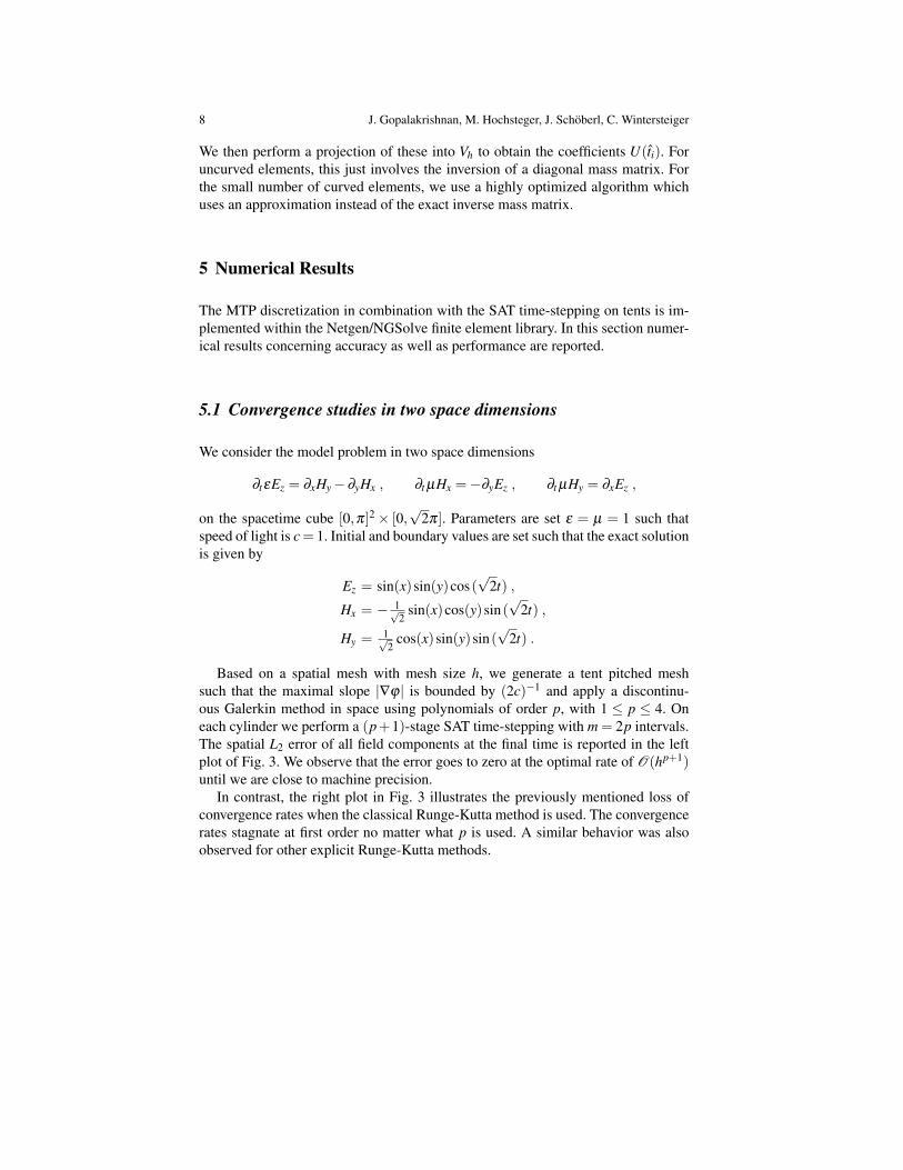
5.1 Convergence studies in two space dimensions
We consider the model problem in two space dimensions
∂tεEz = ∂xHy−∂yHx , ∂t µHx =−∂yEz , ∂t µHy = ∂xEz ,
on the spacetime cube [0,π]2× [0,√
2π]. Parameters are set ε = µ = 1 such thatspeed of light is c= 1. Initial and boundary values are set such that the exact solutionis given by
Ez = sin(x)sin(y)cos(√
2t) ,
Hx = − 1√2
sin(x)cos(y)sin(√
2t) ,
Hy = 1√2
cos(x)sin(y)sin(√
2t) .
Based on a spatial mesh with mesh size h, we generate a tent pitched meshsuch that the maximal slope |∇ϕ| is bounded by (2c)−1 and apply a discontinu-ous Galerkin method in space using polynomials of order p, with 1 ≤ p ≤ 4. Oneach cylinder we perform a (p+1)-stage SAT time-stepping with m = 2p intervals.The spatial L2 error of all field components at the final time is reported in the leftplot of Fig. 3. We observe that the error goes to zero at the optimal rate of O(hp+1)until we are close to machine precision.
In contrast, the right plot in Fig. 3 illustrates the previously mentioned loss ofconvergence rates when the classical Runge-Kutta method is used. The convergencerates stagnate at first order no matter what p is used. A similar behavior was alsoobserved for other explicit Runge-Kutta methods.

MTP scheme for Maxwell Equations 9
103 105 107
10−1
10−3
10−5
10−7
10−9
10−11
10−13
dof
(p+1)-stage SAT time-stepping
p = 1 p = 2 p = 3 p = 4O(h) O(h2) O(h3) O(h4) O(h5)
103 105 107dof
classical Runge-Kutta method
Fig. 3 Spatial L2 error of all field components over degrees of freedom (dof) for the (p+1)-stageSAT time-stepping (left) and the classical Runge-Kutta (right).
5.2 Large scale problem in three space dimensions
As a second example we present a simulation on a domain similar to the resonatorshown in [4]. The geometry is given as body of revolution of smooth B-splinecurves. The mesh consisting of 489593 curved tetrahedral elements is shown inFig. 4. Due to higher curvature the mesh is refined along the inner roundings, wherethe ratio of the largest to the smallest element is approximately 5:1. We used aGaussian peak (located at the axis of revolution and the position of the fifth innerrounding) for the electric field as initial data. The explicit MTP scheme with SATtime-stepping then computed the solution at t = 260 using time slabs of height 1,with each slab composed of Ntents = 149072 tents. On each tent we used a (p+1)-stage SAT time-stepping with m = 2p intervals, where p denotes the spatial polyno-mial order. With the spatial degrees of freedom Ndof,i of the ith tent and the numberof stages q = p+1, we obtain the total spacetime degrees of freedom per time slab
Ntents
∑i=1
Ndof,i mq =
(Ntents
∑i=1
Ndof,i
)2p(p+1) .
The corresponding numbers of degrees of freedom and the simulation times areshown in Table 1. In [4] a similar problem is solved using a discontinuous Galerkinmethod with quadratic elements, combined with a polynomial Krylov subspacemethod in time. Using 96 cores it took them 7:10 hours to reach the final time.Our simulation with polynomial order p = 3, which has a comparable number ofunknowns, took 3:33 hours on 64 cores. This significant speed up is an illustration
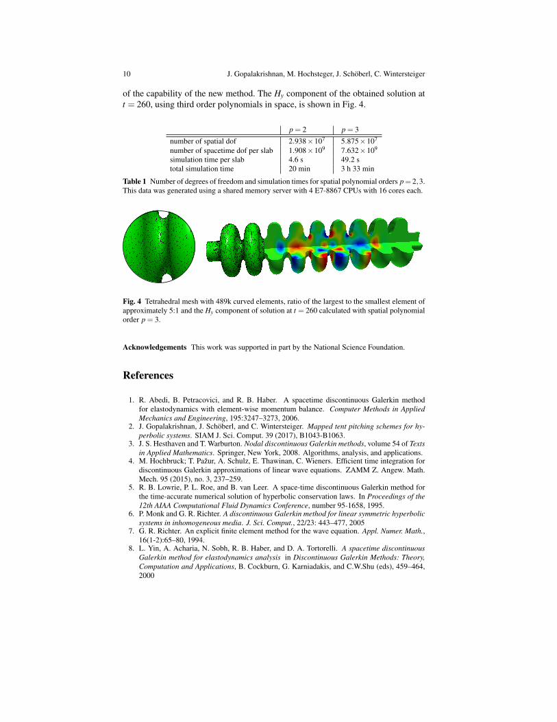
10 J. Gopalakrishnan, M. Hochsteger, J. Schoberl, C. Wintersteiger
of the capability of the new method. The Hy component of the obtained solution att = 260, using third order polynomials in space, is shown in Fig. 4.
p = 2 p = 3number of spatial dof 2.938×10⁷ 5.875×10⁷
number of spacetime dof per slab 1.908×10⁹ 7.632×10⁹
simulation time per slab 4.6 s 49.2 stotal simulation time 20 min 3 h 33 min
Table 1 Number of degrees of freedom and simulation times for spatial polynomial orders p= 2,3.This data was generated using a shared memory server with 4 E7-8867 CPUs with 16 cores each.
Fig. 4 Tetrahedral mesh with 489k curved elements, ratio of the largest to the smallest element ofapproximately 5:1 and the Hy component of solution at t = 260 calculated with spatial polynomialorder p = 3.
Acknowledgements This work was supported in part by the National Science Foundation.
References
1. R. Abedi, B. Petracovici, and R. B. Haber. A spacetime discontinuous Galerkin methodfor elastodynamics with element-wise momentum balance. Computer Methods in AppliedMechanics and Engineering, 195:3247–3273, 2006.
2. J. Gopalakrishnan, J. Schoberl, and C. Wintersteiger. Mapped tent pitching schemes for hy-perbolic systems. SIAM J. Sci. Comput. 39 (2017), B1043-B1063.
3. J. S. Hesthaven and T. Warburton. Nodal discontinuous Galerkin methods, volume 54 of Textsin Applied Mathematics. Springer, New York, 2008. Algorithms, analysis, and applications.
4. M. Hochbruck; T. Pazur, A. Schulz, E. Thawinan, C. Wieners. Efficient time integration fordiscontinuous Galerkin approximations of linear wave equations. ZAMM Z. Angew. Math.Mech. 95 (2015), no. 3, 237–259.
5. R. B. Lowrie, P. L. Roe, and B. van Leer. A space-time discontinuous Galerkin method forthe time-accurate numerical solution of hyperbolic conservation laws. In Proceedings of the12th AIAA Computational Fluid Dynamics Conference, number 95-1658, 1995.
6. P. Monk and G. R. Richter. A discontinuous Galerkin method for linear symmetric hyperbolicsystems in inhomogeneous media. J. Sci. Comput., 22/23: 443–477, 2005
7. G. R. Richter. An explicit finite element method for the wave equation. Appl. Numer. Math.,16(1-2):65–80, 1994.
8. L. Yin, A. Acharia, N. Sobh, R. B. Haber, and D. A. Tortorelli. A spacetime discontinuousGalerkin method for elastodynamics analysis in Discontinuous Galerkin Methods: Theory,Computation and Applications, B. Cockburn, G. Karniadakis, and C.W.Shu (eds), 459–464,2000