Embed Size (px)
Citation preview

An Experimental Study of Five-Coordinate Iron
Complexes Containing Non-Innocent Aminobenzenethiol
Based Ligands
Dissertation for the degree of
Doktor der Naturwissenschaft
in the Fakultät für Chemie
at the Ruhr-Universität Bochum
Presented by
Shaun Richard Presow
Mülheim an der Ruhr, June 2008


This work was independently carried out between April 2005 and April 2008 at the Max-
Planck Insitut für Bioanorganische Chemie, Mülheim an der Ruhr, Germany.
Submitted on: 20 June 2008
Referant: Prof. Dr. K. Wieghardt (Referant)
Koreferant: Dr. N. Metzler-Nolte (Koreferant)

Acknowledgements
I am grateful to many for the support and encouragement they provided me through the course
of this study. I would especially like to acknowledge the following:
Prof. Dr. Karl Wieghardt, for providing me with the opportunity to work within his research
group and the scientific guidance he has provided me with throughout my time in Mülheim an
der Ruhr. I am greatly indebted to him.
Dr Eckhard Bill, for his continual and unstinting help in understanding spectroscopic results.
Dr. Thomas Weyhermüller, for interpretation of single crystal X-ray diffraction data and the
friendly support.
Dr. Richard Mynott, for very helpful discussion of NMR results.
Mr Bernd Mienert, for measurement of Mössbauer data, and friendly discussion over lunch.
Mrs Heike Schucht for collection of single crystal X-ray diffraction date.
Mr Jörg Bitter and Mrs Kerstin Neurieder for collection of NMR results.
Mr Frank Reikowski, for measurement of EPR data.
Mr Andreas Göbels, for measurement of SQUID data.
Mrs Ursula Westhoff, for collection of GC-MS results.
Drs. Connie Lu, Jennifer Shaw and Geoff Spikes, For endless help and advice in the lab, as
well as revision of the manuscript.
Special thanks to my officemates, Flavio Benedito and Carsten Milsmann for many
productive discussions.

Of course this work could not have been done without the help and support of my laboratory
colleagues, Drs. Nuria Aliaga-Alcade, John Berry, Krzysztof Chłopek, Prasanta Ghosh,
Corinna Hess, Ruta Kapre, Marik Khusniyarov, Melissa Koay, Nicolleta Muresan, József
Pap, Kallol Ray, Stephen Sproules, Isabelle Sylvestre, and Messrs Biplab Biswas, Michael
Nippe, Bram Pluijmaekers and Nabarun Roy.
To my parents, John and Sue Presow and their endless love and support, as well as that
provided by my sisters Rebecca and Kimberley.
Jamie Morris, without whose encouragement and love this project would never have been
begun, let alone completed.
I am also grateful to the Max-Planck-Gesellschaft (MPG) for financial support.

For Jamie

I
Contents
Chapter 1 Introduction 1
1.0. The concept of physical and formal oxidation states 3
1.1. Non-innocent ligands 4
1.2. Dithiolenes and 1,2-benzenedithiols 5
1.3. o-Phenylenediamines 7
1.4. o-Aminothiophenols 9
1.5. α-Dimines 11
1.6. Glyoxal-bis(2-mercaptoaniline) 12
1.7. Objectives 15
Chapter 2 Dimeric Complexes of Iron Containing a Tetradentate
o-Iminothionesemiquinonate Ligand
19
2.0. Introduction 21
2.1. [Fe(1L•)]2 (1) 23
2.2. [Fe(2L•)]2 (2) 28
2.3. DFT calculations of 1 and 2 38
Chapter 3 Square Pyramidal Complexes of Iron Containing Tetradentate
o-Iminothionesemiquinonate Ligands and an Apical Iodide
47
3.0. Introduction 49
3.1. [Fe(1L••)I] (3) 51
3.2. [Fe(2L••)I] (4) 61
3.3. DFT calculations of 3 and 4 68
Chapter 4 Square Pyramidal Complexes of Iron Containing a
Tetradentate o-Iminothionesemiquinonate and Apical
Phosphine or Phosphite Ligands
75
4.0. Introduction 77
4.1. Synthesis of [Fe(1L••)(P(CH3)3)] (5), [Fe(1L••)(P(OCH3)3)]
(6), [Fe(1L••)(P(C6H5)3)] (7), [Fe(1L••)(P(OC6H5)3)] (8),
[Fe(2L••)(P(C6H5)3)] (9) and [Fe(2L••)(P(OC6H5)3)] (10).
79
4.2. Crystal structure determination of 5, 6, 7, 8, 9 and 10 79
4.3. Electronic absorption spectroscopy 88

II
4.4. Mössbauer spectroscopy 91
4.5. Nuclear magnetic resonance spectroscopy 94
4.6 DFT calculations of 5 and 6 109
Chapter 5 A Square Pyramidal Complex of Iron Containing a
Tetradentate bis(o-Iminothionebenzosemiquinonate) and an
Apical tert-Butylpyridine Ligand
115
5.0. Introduction 117
5.1. [Fe(2Lgma•)(t-Bupy) (11) 119
Chapter 6 Conclusion 133
Chapter 7 Methods and Equipment 141
Chapter 8 Experimental 149
Chapter 9 Bibliography 169
Chapter 10 Appendix 179
III
List of abbreviations and symbols
abt aminobenzenethiol
A hyperfine coupling constant
Å angstrom
B magnetic field
B3LYP Becke 3-parameter (exchange), Lee, Yang and Parr (correlation; DFT)
bdt o-benzenedithiol
br broad
Bu butyl
cm centimetre
CT charge transfer
d doublet
D axial zero-field splitting parameter
DFT density functional theory
dpdt 1,2-diphenyl-1,2-dithiolene
e electron
edbt 1,2-ethanediamine-N,N’-bis(2-benzenethiol)
E/D rhombicity
eff effective
EFG electric field gradient
EI electron ionisation
EPR electron paramagnetic resonance
ESI electrospray ionisation
g electron Lande factor
gN nuclear Lande factor
G gauss
GC gas chromatography
GHz gigahertz
gma glyoxal-2-bis(mercaptoaniline)
H Hamiltonian operator
HOMO highest occupied molecular orbital
Hz hertz
I nuclear quantum number
IR infrared

IV
ISO isotropic
IVCT intervalence charge transfer
J coupling constant
k = kB Boltzmann constant
K Kelvin
LLCT ligand-to-ligand charge transfer
LMCT ligand-to-metal charge transfer
LUMO lowest unoccupied molecular orbital
m metre (or multiplet in NMR)
mm millimetre
mnt maleonitriledithiolene
M molar = mol dm-3
Me methyl
MHz megahertz
MO molecular orbital
nm nanometre
N Avogadro constant
NMR nuclear magnetic resonance
Ph phenyl
py pyridine
q quartet
Q quadrupole moment
R gas constant
RT room temperature
s second (or singlet in NMR)
S local spin state (or spin quantum number)
SOMO singly occupied molecular orbital
SQUID superconducting quantum interference device
ST total spin state
t triplet
T Tesla
tdt toluenedithiol
tert = t tertiary
TIP temperature independent paramagnetism
V
UV-vis ultraviolet-visible
Vij EFG component
βN = µN nuclear magneton
Γ line width
δ isomer shift in NMR (or isomer shift in Mössbauer spectroscopy)
∆EQ quadrupole splitting
∆H enthalpy change
∆S entropy change
σ standard deviation
ε extinction coefficient
η asymmetry parameter
θ Weiss constant
λ wavelength
µ dipole moment
µB Bohr magneton
ν frequency
χmol molar susceptibility
SH
NH HN
HSSH
NH HN
HS
1LH4 2LH4
VI
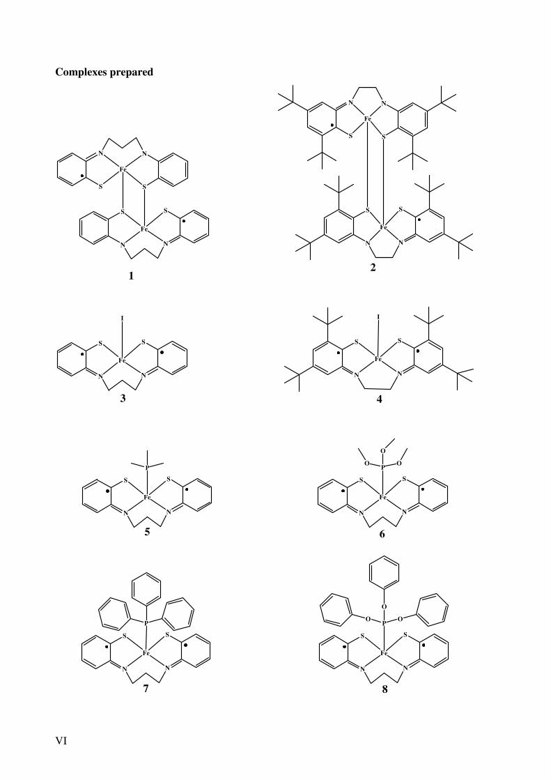
Complexes prepared
N
S
N
S
Fe
N
S
N
S
Fe
N
S
N
S
Fe
N
S
N
S
Fe
I
N
S
N
S
Fe
I
N
S
N
S
Fe
P
N
S
N
S
Fe
P
N
S
N
S
Fe
O
O
O
P
N
S
N
S
Fe
P
N
S
N
S
Fe
O
O
O
1 2
3 4
5 6
7 8
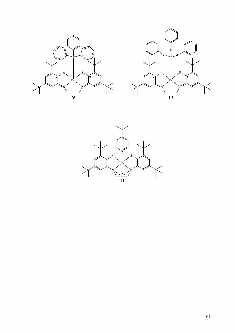
VII
N
S
N
S
FeI
P
N
S
N
S
FeI
P
O
OO
N
S
N
S
FeI
N
9 10
11

VIII

1
CHAPTER 1
Introduction

2

Chapter 1
3
1.0 The concept of physical and formal oxidation states
It has been well known for some time that transition metal ions play a crucial role in biology,
most interestingly at or near the active sites of a wide range of enzymes. Indeed, the first
protein ever crystallised, urease, was later found to contain a bimetallic nickel(II) active site.1-
3 A classic example of a metalloenzyme (due to it being well understood) is that of galactose
oxidase, in which the active enzyme features a copper(II) ion directly coordinated to a
modified tyrosyl radical. This enzyme is responsible for the two electron oxidation of a sugar
based hydroxyl group to an aldehyde, with hydrogen peroxide formed as a byproduct.4
Mechanisms involving radicals have been implicated in a wide variety of enzymatic reactions,
including those involving vitamin B12, amine oxidases and peroxidases.5 Further as yet
undiscovered reactions mechanisms might utilise coordinated radicals, yet the detection of
these is not trivial. Strong coupling between a coordinated radical and the metal centre can
obscure the presence of the radical, while structural indicators from techniques such as low
temperature X-ray crystallography are much more difficult to obtain. Thus an examination of
small model compounds containing ligand-based radicals is warranted, in order to determine
bonding properties and physical characteristics of coordinated radicals, with the idea that this
knowledge may be of use in elucidating the reactivity and mechanisms of metalloenzymes.
One complication to this is the inconsistency which sometimes occurs between a
metal’s formal oxidation state, and its physical (or spectroscopic) oxidation state. The formal
oxidation state is an immeasurable integer which is defined as the charge remaining on the
metal ion after that of the closed-shell ligand is accounted for.6 It has also been suggested that
a number arising from the d electron configuration of the metal should be defined as the
physical oxidation number.7 Thus the oxidation number would be related to the number of d
electrons at the metal ion, which it is possible to measure using a variety of spectroscopic
techniques.
Generally the formal and physical oxidation states of a metal in a metal complex are
identical. The situation is somewhat complicated however when the ligand is also redox
active. A non-innocent ligand with an open-shell configuration (such as a π radical)
coordinated to a central metal ion leads to a difference between the formal and physical
oxidation states. An example of this is galactose oxidase, where a copper centre is bound to a
phenoxyl-type radical (Ar-O•). The physical oxidation state of the copper has been
characterised as +2, with nine d electrons.4 However, the formal oxidation state of the metal
requires that the radical be treated as a closed-shell phenolate(-1), which in turn implies that
the copper has a (+3) formal oxidation state. In this case the formal oxidation state is an

Chapter 1
4
unphysical assumption, whereas the physical oxidation state more accurately reflects the
bonding situation.
This distinction is an important one, and a failure to recognise the difference between
formal and physical oxidation states can lead to the mistaken characterisation of complexes,
such as iron(IV)8,9 and iron(V)10 complexes initially reported in 1997, where in fact the
compounds were later found11 to contain Fe(II) and Fe(III) complexed to open-shell ligands
containing π radicals.
1.1 Non-innocent ligands
Typically for transition metal compounds, the frontier molecular orbitals are those of the
valence d-shell of the metal. In these cases, any redox process will take place at the metal
centre and will change the formal oxidation state of the metal. However, depending on the
nature of the ligand, the frontier molecular orbitals (MOs) can be mostly ligand based. In
these cases any redox process will add or remove electrons from a ligand-based orbital, and
the oxidation level of the ligand will change while that of the metal will remain constant. This
is shown in Figure 1.1.1,12 which demonstrates the frontier orbitals of the two situations
discussed. The situation on the left is that typically observed, where the singly occupied MO
is primarily metal in nature. Presented on the right is a situation where the singly occupied
MO is primarily ligand based, and oxidation or reduction will take place in this orbital. Thus
any redox process will be chiefly ligand based.
Figure 1.1.1. Simplified MO scheme describing the normal
bonding scheme between a transition metal and ligand (left),
and the situation observed with a non-innocent ligand (right).
Metal
d orbital
Metal
d orbital
Ligand
orbital
Ligand
orbital

Chapter 1
5
This situation can arise when the ligand molecular orbitals are raised in energy or the metal
based orbitals are lowered in energy. More and more ligand classes which exhibit non-
innocent behaviour are being identified, both through novel synthesis and a re-examination of
previously synthesised compounds. The ligands relevant to this work can be classed into
several groups, which are discussed separately below.
1.2. Dithiolenes and 1,2-benzenedithiols
Dithiolene and 1,2-benzenedithiolate ligands have a long history in coordination chemistry,
with the first dithiolene complexes being synthesised using maleonitriledithiolate(-2) (mnt)
and 1,2-diphenyl-1,2-dithiolene (dpdt). The complexes were reported in the early 1960s by
the groups of Schrauzer et al.13 and Gray et a.,14 and both complexes were originally
characterised as containing a central Ni(II) ion (Figure 1.2.1).
S
S S
S
Ni
Figure 1.2.1. First dithiolene complexes synthesised by
Schrauzer et al. (left) and Gray et al. (right).
Further work by Holm et al. included the use of the –CF3 substituted dithiolene ligand
((CF3)2C2S2), and led to the isolation of neutral Ni, Pd and Pt bis complexes featuring one of
the three dithiolene ligands. Electrochemistry experiments revealed a three-member redox
series for each of the compounds consisting of the neutral complex, a monoanion and a
dianion.15,16 Exact structures of the complexes could not be determined, but all were believed
to be isostructural. The neutral and dianionic species were found to be diamagnetic, but the
monoanions were paramagnetic with a S = ½ ground state.
o-Benzenedithiol (bdt) and toluenedithiol (tdt) containing nickel complexes, also
synthesised in the 1960s, show similar redox behaviour.17 The synthesis of cobalt and iron
complexes with dithiolene based ligands led to the characterisation of dimeric compounds,
[Co(S2C2(CF3)2)2]2 and [Fe(S2C2(CF3)2)2]2.18,19 The iron dimer was not confirmed by single
crystal X-ray diffraction, but it was inferred from the data collected on the cobalt complex to
S
NC S CNS
CNS
Ni
NC
-2
Chapter 1
6
be isostructural. The first concrete evidence of the dimeric nature of the dithiolene iron
complexes was through X-ray crystal analysis of (n-Bu4N)2[Fe(mnt)2]2 in 1967.20 However,
the electronic structures of these compounds remained elusive. The distinct structural
parameters we now recognise as being so important to the classification of the electronic
structure of the ligand were observed in 1967,19 though conclusive evidence for the electronic
structure of the complex remained elusive. The Mössbauer data for a large number of
dithiolene and o-benzenedithiol iron complexes were reported and it was found that the
isomer shift did not deviate greatly, even upon oxidation. This provided evidence that the
redox processes were occurring not at the central metal, but at the ligands.21
Debate on the nature of these compounds continued for the next four decades. As
recently as 2000, it was claimed that for the series of square planar nickel complexes [Ni(tBu-
bdt)2]0,1-,2- (tBu-bdt = 3,5-di-tert-butylbenzene-1,2-dithiolate) the ligands remain throughout in
the closed-shell 1,2-dithiolate(2-) redox state. This in turn requires that the nickel centre be
characterised as Ni(II), Ni(III) and Ni(IV) in the dianionic, monoanionic and neutral species
respectively.22 Several recent publications have refuted this proposal, demonstrating through
the use of density functional theory (DFT) and ab initio methods, as well as spectroscopic
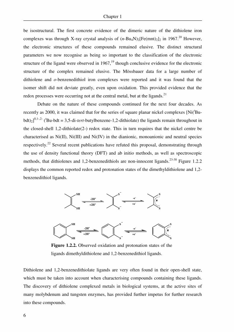
methods, that dithiolenes and 1,2-benzenedithiols are non-innocent ligands.23-30 Figure 1.2.2
displays the common reported redox and protonation states of the dimethyldithiolene and 1,2-
benzenedithiol ligands.
SH
SH
S
S
S
S
-2H+
+2H+
-e-
+e-
SH
SH
S
S
S
S
-2H+
+2H+
-e-
+e-
Figure 1.2.2. Observed oxidation and protonation states of the
ligands dimethyldithiolene and 1,2-benzenedithiol ligands.
Dithiolene and 1,2-benzenedithiolate ligands are very often found in their open-shell state,
which must be taken into account when characterising compounds containing these ligands.
The discovery of dithiolene complexed metals in biological systems, at the active sites of
many molybdenum and tungsten enzymes, has provided further impetus for further research
into these compounds.
Chapter 1
7
1.3. o-Phenylenediamines
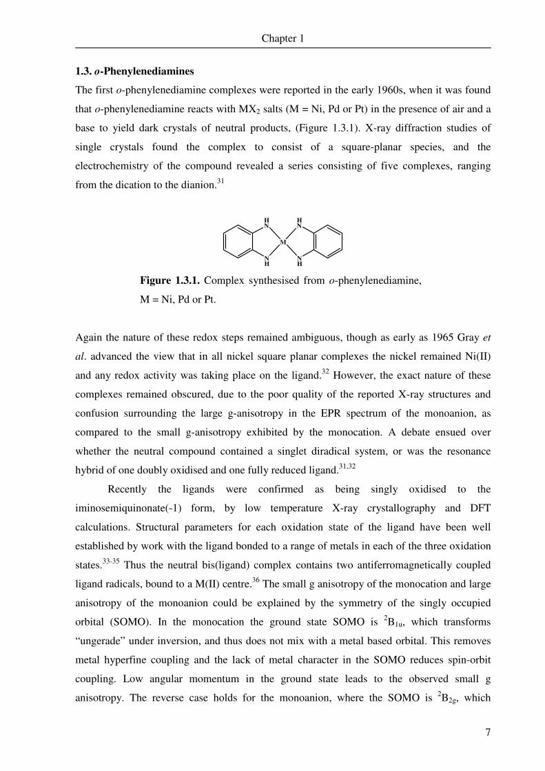
The first o-phenylenediamine complexes were reported in the early 1960s, when it was found
that o-phenylenediamine reacts with MX2 salts (M = Ni, Pd or Pt) in the presence of air and a
base to yield dark crystals of neutral products, (Figure 1.3.1). X-ray diffraction studies of
single crystals found the complex to consist of a square-planar species, and the
electrochemistry of the compound revealed a series consisting of five complexes, ranging
from the dication to the dianion.31
HN
NH
NH
HN
M
Figure 1.3.1. Complex synthesised from o-phenylenediamine,
M = Ni, Pd or Pt.
Again the nature of these redox steps remained ambiguous, though as early as 1965 Gray et
al. advanced the view that in all nickel square planar complexes the nickel remained Ni(II)
and any redox activity was taking place on the ligand.32 However, the exact nature of these
complexes remained obscured, due to the poor quality of the reported X-ray structures and
confusion surrounding the large g-anisotropy in the EPR spectrum of the monoanion, as
compared to the small g-anisotropy exhibited by the monocation. A debate ensued over
whether the neutral compound contained a singlet diradical system, or was the resonance
hybrid of one doubly oxidised and one fully reduced ligand.31,32
Recently the ligands were confirmed as being singly oxidised to the
iminosemiquinonate(-1) form, by low temperature X-ray crystallography and DFT
calculations. Structural parameters for each oxidation state of the ligand have been well
established by work with the ligand bonded to a range of metals in each of the three oxidation
states.33-35 Thus the neutral bis(ligand) complex contains two antiferromagnetically coupled
ligand radicals, bound to a M(II) centre.36 The small g anisotropy of the monocation and large
anisotropy of the monoanion could be explained by the symmetry of the singly occupied
orbital (SOMO). In the monocation the ground state SOMO is 2B1u, which transforms
“ungerade” under inversion, and thus does not mix with a metal based orbital. This removes
metal hyperfine coupling and the lack of metal character in the SOMO reduces spin-orbit
coupling. Low angular momentum in the ground state leads to the observed small g
anisotropy. The reverse case holds for the monoanion, where the SOMO is 2B2g, which
Chapter 1
8
transforms “gerade” and has a large metal contribution. Consequently hyperfine coupling
from the metal is observed as well as a large g anisotropy. Combined with careful analysis of
the electronic spectra of the series, the redox activity of the complex was shown to be
completely ligand based, as had been suggested by Gray et al. in 1965.32 The redox series for
the nickel complex is shown in Figure 1.3.2.
HN
NH
NH
HN
Ni
HN
NH
NH
HN
Ni
HN
NH
NH
HN
Ni
HN
NH
NH
HN
Ni
HN
NH
NH
HN
Ni
-e-
+e--e-
+e-
-e-+e-
-e-
+e-
Figure 1.3.2. Redox series of [Ni(o-pda)2]2+,1+,0,1-,2- (o-pda =
o-phenylenediamine).
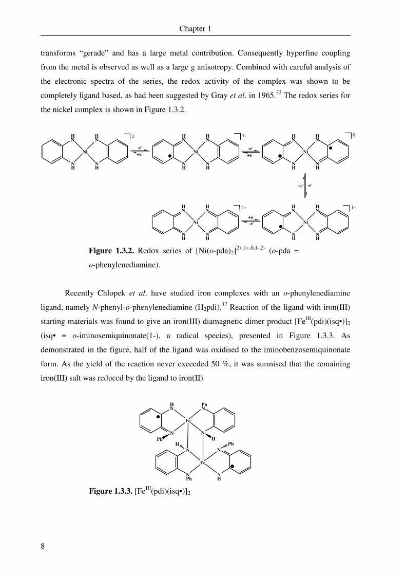
Recently Chlopek et al. have studied iron complexes with an o-phenylenediamine
ligand, namely N-phenyl-o-phenylenediamine (H2pdi).37 Reaction of the ligand with iron(III)
starting materials was found to give an iron(III) diamagnetic dimer product [FeIII(pdi)(isq•)]2
(isq• = o-iminosemiquinonate(1-), a radical species), presented in Figure 1.3.3. As
demonstrated in the figure, half of the ligand was oxidised to the iminobenzosemiquinonate
form. As the yield of the reaction never exceeded 50 %, it was surmised that the remaining
iron(III) salt was reduced by the ligand to iron(II).
HN
N N
PhN
Fe
Ph H
NH
NN
NPh
Fe
PhH
Figure 1.3.3. [FeIII(pdi)(isq•)]2
2+ 1+
0 1- 2-
Chapter 1
9
The diamagnetic complex was studied with Mössbauer spectroscopy, X-ray diffraction
crystallography and UV-vis spectroscopy. It was found that the iron(III) had an intermediate
spin state, with strong antiferromagnetic coupling between the adjacent iron and radical
centres, and between the two iron ions.
The dimeric species proved to be a useful starting material for a wide range of
five-coordinate square-pyramidal compounds. These complexes could be completely
characterised spectroscopically and, depending on the ligand chosen to break the dimer, the
iron was found to be either Fe(II) or Fe(III) bound to two ligand-based π radicals. The
iron(III) complexes were found to be universally intermediate spin, as is expected for the
square-pyramidal geometry. Several markers were identified that indicate the presence of a
diradical species and an intermediate spin iron(III), which assist in identifying the physical
oxidation number of the metal centre. In particular these were the identification of the
particular hyperfine coupling parameters of the intermediate spin iron(III) core, obtained
through applied field Mössbauer spectroscopy, which consist of two large positive and one
small negative contribution in square-pyramidal complexes.38 The inverse is observed in
octahedral complexes, which have one small positive and two large negative contributions.
Additionally, the presence of a diradical species with perfectly parallel π-systems can be
inferred by the intense (ε > 10,000) ligand-to-ligand charge transfer bands observed in the
electronic spectra of these complexes.38
1.4. o-Aminothiophenols
The first o-aminothiophenol (abt) complexes were synthesised in anaerobic conditions in
1968,39 though the structures of the various metal complexes remained ambiguous. The first
reported structure containing abt was a dimeric species [Fe2(abt)(CO)6], where a single abt
ligand was coordinated to both iron centres.40 In this case, it is apparent from ligand bond
parameters that it is a closed-shell dianion. As for the benzenedithiols and
o-phenylenediamine complexes, there was considerable interest in the physical and electronic
structure of these compounds. A dimeric iron species containing the substituted abt ligand
4,6-di-tert-butyl-2-aminothiophenol(2-) was reported in 2003 (Figure 1.4.1).41

Chapter 1
10
H2N
S S
H2N
Fe
S
NH2
NH2
S
Fe
t-Bu
t-Bu
t-Bu
t-Bu
t-Bu
t-Bu
t-Bu
t-Bu
Figure 1.4.1. Structures of iron dimer complexes containing
abt based ligands.
Controversy over the electronic structure erupted over the publication of two reports in which
it was claimed that the abt based ligand 1,2-ethanediamine-N,N’-bis(2-benzenethiol)(4-)
(edbt) stabilised unusually high oxidation states for iron, namely iron(IV) and iron(V). The
two complexes in question, shown in Figure 1.4.2, were neutral square-pyramidal iron
complexes with an apical ligand, either a phosphine or an iodide.8,10
S
N N
S
FeIV
S
N N
S
FeV
PR
R
R
I
Figure 1.4.2. Complexes characterised as either an iron(IV)
complex (left) or an iron(V) complex (right). R = phenyl or n-
propyl groups.
Complete characterisation of square-planar nickel(II), palladium(II) and platinum(II)
complexes containing either tert-butyl substituted or unsubstituted abt based ligands revealed
the non-innocent nature of the ligand, which could be oxidised to give the
o-iminothionebenzosemiquinonate(1-) (isq•) form.36,42 Further examination of the supposed
iron(IV) and iron(V) complexes, particularly through the use of high quality single crystal X-
ray diffraction analysis, Mössbauer spectroscopy, EPR spectroscopy and DFT calculations led
to a reassessment of the complexes as containing either an iron(II) or an iron(III) ion bound to
a ligand that has been doubly oxidised to give two o-iminothionebenzosemiquinonate(1-) π
radicals (Figure 1.4.3).11,43,44

Chapter 1
11
S
N N
S
FeII
S
N N
S
FeIII
PR
R
R
I
Figure 1.4.3. Electronic structure of two complexes after
reassignment through spectroscopic and computational
methods. R = phenyl.
It has thus been well demonstrated that ligands containing an abt type manifold are non-
innocent, and the open-shell form of the ligands can be identified through X-ray crystal
diffraction, spectroscopic examination and DFT calculation.
1.5. α-Diimines
A further class of non-innocent ligands is that of 1,2-diimines. α-Diimines can be reduced by
one electron to give a radical species, and further singly reduced to give the closed-shell
dianion. This redox series is presented in Figure 1.5.1.
N
N
0
+e-
-e-
N
N
1-
N
N
2-
+e-
-e-
Figure 1.5.1. Redox series of diimine ligands.
In order to exclude the effect of d-orbitals these systems have been studied using main group
metal ions, in particular lithium.45 Utilising X-ray crystallography, the complexes could be
readily characterised as containing redox active ligands. As the oxidation state of the ligand
changes, so do the ligand C-N and C-C bond lengths. This change can be examined directly in
high quality X-ray crystal structures. Despite this, there are several published reports in which
neutral α-diimine iron complexes are described as containing an Fe0 centre coordinated to two
closed-shell diimine ligands.46-48 It has now been shown conclusively in the literature that α-
diimine ligands are non-innocent, and are reduced to the π radical monoanionic forms within
iron, nickel or zinc neutral bis complexes.49-52
Chapter 1
12
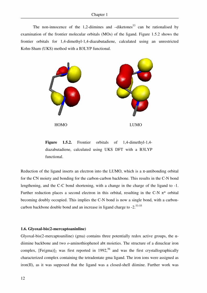
The non-innocence of the 1,2-diimines and –diketones53 can be rationalised by
examination of the frontier molecular orbitals (MOs) of the ligand. Figure 1.5.2 shows the
frontier orbitals for 1,4-dimethyl-1,4-diazabutadiene, calculated using an unrestricted
Kohn-Sham (UKS) method with a B3LYP functional.
Figure 1.5.2. Frontier orbitals of 1,4-dimethyl-1,4-
diazabutadiene, calculated using UKS DFT with a B3LYP
functional.
Reduction of the ligand inserts an electron into the LUMO, which is a π-antibonding orbital
for the CN moiety and bonding for the carbon-carbon backbone. This results in the C-N bond
lengthening, and the C-C bond shortening, with a change in the charge of the ligand to -1.
Further reduction places a second electron in this orbital, resulting in the C-N π* orbital
becoming doubly occupied. This implies the C-N bond is now a single bond, with a carbon-
carbon backbone double bond and an increase in ligand charge to -2.53-55
1.6. Glyoxal-bis(2-mercaptoaninline)
Glyoxal-bis(2-mercaptoaniline) (gma) contains three potentially redox active groups, the α-
diimine backbone and two o-aminothiophenol abt moieties. The structure of a dinuclear iron
complex, [Fe(gma)]2 was first reported in 1992,56 and was the first crystallographically
characterized complex containing the tetradentate gma ligand. The iron ions were assigned as
iron(II), as it was supposed that the ligand was a closed-shell diimine. Further work was
LUMO HOMO
Chapter 1
13
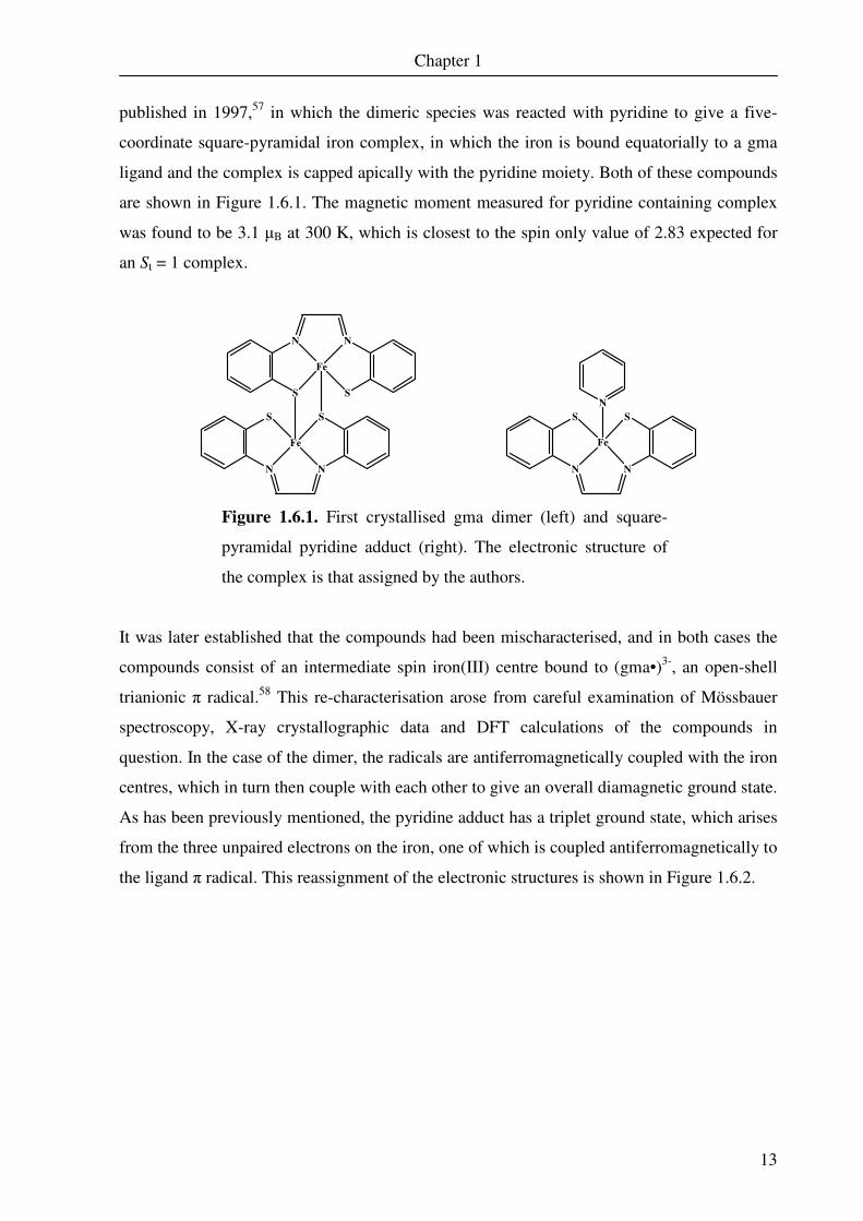
published in 1997,57 in which the dimeric species was reacted with pyridine to give a five-
coordinate square-pyramidal iron complex, in which the iron is bound equatorially to a gma
ligand and the complex is capped apically with the pyridine moiety. Both of these compounds
are shown in Figure 1.6.1. The magnetic moment measured for pyridine containing complex
was found to be 3.1 µB at 300 K, which is closest to the spin only value of 2.83 expected for
an St = 1 complex.
S
N N
S
Fe
S
N N
S
Fe
S
N N
S
Fe
N
Figure 1.6.1. First crystallised gma dimer (left) and square-
pyramidal pyridine adduct (right). The electronic structure of
the complex is that assigned by the authors.
It was later established that the compounds had been mischaracterised, and in both cases the
compounds consist of an intermediate spin iron(III) centre bound to (gma•)3-, an open-shell
trianionic π radical.58 This re-characterisation arose from careful examination of Mössbauer
spectroscopy, X-ray crystallographic data and DFT calculations of the compounds in
question. In the case of the dimer, the radicals are antiferromagnetically coupled with the iron
centres, which in turn then couple with each other to give an overall diamagnetic ground state.
As has been previously mentioned, the pyridine adduct has a triplet ground state, which arises
from the three unpaired electrons on the iron, one of which is coupled antiferromagnetically to
the ligand π radical. This reassignment of the electronic structures is shown in Figure 1.6.2.

Chapter 1
14
S
N N
S
FeIII
S
N N
S
FeIII
S
N N
S
FeIII
N
Figure 1.6.2. Electronic structure of the neutral gma dimer and
pyridine adduct.
It has been noted that it is possible to obtain a gma type ligand from the abt derived ligand
1,2-ethanediamine-N,N’-bis(2-benzenethiol) (H4edbt) through deprotonation and oxidation.59
This demonstrates that ethyl-bridged abt ligands contain three possible redox states, which
complicates assignment of the physical oxidation state for the metal. Scheme 1.6.1 presents
some of the available redox and protonation states for edbt.
SH
NH HN
HS S
N N
S S
N N
S
S
N N
SS
N N
SS
N N
S
-4H+
+4H++e-
-e-
-e-+e-
-2H+, -e-
+2H+, +e-+e-
-e-
H
H
H
H
H H
H H
H
H
H
H
H H
H
HHHH
H
Scheme 1.6.1. Protonation and oxidation states of
1,2-ethanediamine-N,N’-bis(2-benzenethiol), showing the
electronic rearrangement upon deprotonation to give (gma•)3-.
H4edbt
gma•-3
edbt-4
gma-2

Chapter 1
15
1.7. Objectives of this thesis
The goal of this work was to investigate the effect of conjugation or saturation of the diimine
backbone on electronic communication between the two sides of tetradentate
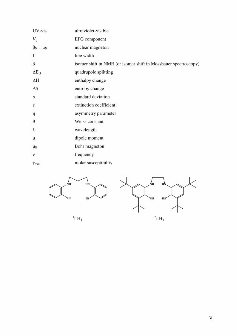
aminobenzenethiol based ligands. To that end two ligands were synthesised and characterised,
1,3-propanediamine-N,N’-bis(2-benzenethiol) (1LH4) and 1,2-bis(2-mercapto-3,5-di-tert-
butylaniline)ethane (2LH4), as shown in Figure 1.7.1. 2LH4 was synthesised using the elegant
route developed by Sellmann et al.,60 while 1LH4 could be readily synthesised by a two step
process from 2-hydroxybenzothiazole and 1,3-dibromopropane.
SH
NH HN
HSSH
NH HN
HS
Figure 1.7.1. Structures of the ligands employed in this work.
As previously discussed, both of these ligands are non-innocent and can be singly or doubly
oxidised, generating either one or two ligand-based π radicals. In addition, 2LH4 can be
further oxidised and deprotonated, leading to a rearrangement in which the ligand becomes
“gma” like, containing a π radical in the bridging moiety. In contrast, the backbone of 1LH4
should be redox innocent.
It should be noted that the diagrams of the abt radical system often reflect only one
possible resonance structure, whereas several can be drawn ( Figure 1.7.2).
S
N
R
S
N
R
S
N
R
S
N
R
S
N
R
S
N
R
S
N
R
S
N
R
Figure 1.7.2. Resonance structures of a modified
o-iminothionebenzenesemiquinonato(1-) ligand.
1LH4 2LH4
Chapter 1
16
Use of 1LH4 precludes the formation of a “gma” type adduct, and removes the possibility of
communication between the ligand π radicals in each ring with one another through the
bridging moiety. Any communication that does occur must therefore be through the metal
centre. 2LH4 was chosen as a ligand which could access a “gma” type adduct. Furthermore,
many of the iron complexes of unsubstituted abt ligands suffer from very low solubility. The
tertiary butyl groups of 2LH4 provide much greater solubility, allowing measurement of
solution Mössbauer spectra.
Various tools have proven to be very useful in the rigorous characterisation of ligand-
based radicals. Low temperature X-ray crystallography with good quality crystals allows
determination of a radical system, due to the delocalisation of the radical across the ring. The
presence of a ligand π radical creates very clear distortion of the aromatic bond lengths away
from the typical length of 1.40 Å. Additionally, the structure of the o-
iminothionebenzenesemiquinonato ligand shows shorter than typical bond lengths between
the aromatic ring and nitrogen and sulfur groups. In the case of “gma” type structures, the
bond lengths in the aromatic ring return to more typical values, while those of the bridging
group shorten dramatically. Interestingly, it appears that the bond lengths between the iron
centre and the ligand are not useful in identifying the physical oxidation state of the iron.
Mössbauer spectroscopy is a useful tool for the identification of any iron coordination
compound, but also provides some very specific data for the identification of an open-shell
ligand. It has been shown that the isomer shift of the iron centre does not necessarily shift as
dramatically as one might expect upon oxidation of the iron centre, producing difficulties in
assignation of a spectroscopic oxidation state.11,58 This is especially an issue with the square-
pyramidal iron(II) and iron(III) adducts of abt containing an apical phosphine or iodide. In
these cases, applied-field Mössbauer measurementswere performed to provide more
conclusive assignment of the electronic structure at the iron centre.
Proton and carbon NMR are useful in the characterisation of diamagnetic compounds,
but in the spectra of diamagnetic complexes containing non-innocent abt ligands interesting
shifts appear, which led to the characterisation of several complexes as being paramagnetic.8
This effect is observed in both the dimeric structures, as well as square-pyramidal monomers
containing an apical phosphine group.
The non-innocent nature of 1LH4 and 2LH4 becomes clear upon examination of the
occupied molecular orbitals of the dianionic deprotonated abt obtained from DFT
Chapter 1
17
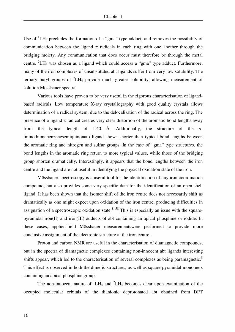
calculations, as has been discussed in the case of 1,2-diimines. The HOMO and HOMO-1 of
abt are shown in Figure 1.7.3.
Figure 1.7.3. Doubly occupied HOMO (left) and HOMO-1
(right) orbitals of the doubly deprotonated dianionic abt ligand,
calculated using UKS DFT with the B3LYP functional.
The HOMO is a doubly occupied orbital, spread across the ring and involving the pz orbitals
of the nitrogen and sulfur. In contrast to this, the HOMO-1 is a sulfur based orbital, which is
responsible for the σ bonding to a metal centre. Upon oxidation an electron is removed from
the HOMO, leaving a ligand π-radical based in the aromatic ring. The changes in bond
lengths observed are also reflected in this orbital, as removal of a bonding electron leads to
extension of the four bonds containing π bonding character, giving rise to the semiquinoidal
pattern of bond lengths. Additionally, the HOMO has π antibonding character between the
ring and the two heteroatoms. Oxidation removes some of this antibonding character, leading
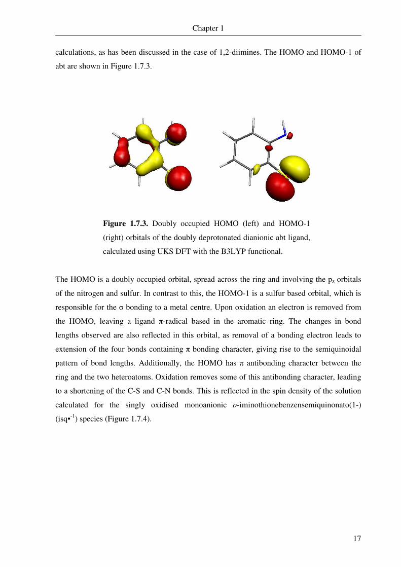
to a shortening of the C-S and C-N bonds. This is reflected in the spin density of the solution
calculated for the singly oxidised monoanionic o-iminothionebenzensemiquinonato(1-)
(isq•-1) species (Figure 1.7.4).
Chapter 1
18
Figure 1.7.4. Spin density obtained from UKS DFT calculation
of isq•-1, utilising the B3LYP functional.
Thus, this work will combine structural data, spectroscopic characterisation and DFT
calculations to investigate the electronic structures of a number of complexes containing the
redox non-innocent 1LH4 and 2LH4.
0.33
0.39
0.16 0.15
0.12
-0.09
19
CHAPTER 2
Dimeric Complexes of Iron
Containing a Tetradentate
o-Iminothionebenzosemiquinonate Ligand

20

21
2.0. Introduction
Dimeric compounds containing two five-coordinate square-pyramidal iron centres are known
in the literature, and have been extensively characterised. The first examples of these
appeared in the literature in the late 1960s. Previous work had found that cobalt compounds
of this type had a dimeric structure.19 Although it was presumed the isostructural iron
compounds were also dimeric,18 the first concrete evidence for discrete dimeric structures for
square-pyramidal iron complexes was provided by the X-ray crystal structure of (n-
Bu4N)2[Fe(mnt)2]2, (where mnt = (NC)2C2S2), obtained by Hamilton et al. in 1967.20 Further
examples were synthesised and characterised by Holm et al., and exclusively consisted of
iron complexed with dithiolene-based ligands to give [FeL2]2, where L = 1,2-disubstituted
ethylene-1,2-dithiolene, 1,2-benzeneditiolate (also referred to as bdt) or 3,4-toluenedithiolate
(tdt).61
The crystal structure and electrochemistry of (n-Bu4N)2[Fe(tdt)2]2 were not published
until 1986,62 followed by the crystal structure of (Et4N)2[Fe(bdt)2]2, published in 1988.63
Extensive work has been carried out on complexes of this type containing sulfur-based or
nitrogen-based ligands.27,37,64-67 The chemistry of complexes of iron with o-
aminobenzenethiol (abt) ligands are now well characterised, with the synthesis and
characterisation of the (µ-S,S)[FeII(abt)2]2 dimer reported in 1968.39 It was assumed abt based
ligands were redox innocent, that is, they did not undergo reduction or oxidation. However, it
has recently been shown that this is not the case, as is shown in Scheme 2.0.1. The ligands
have been identified in several oxidation and protonation states, the most interesting of which
is the o-iminothionebenzosemiquinonate(1-) π radical.68,69
NH
S
NH2
S
NH
S
Scheme 2.0.1. Oxidation and protonation levels identified for
the ligand 1,2-aminobenzenethiol.
This work was extended, where iron complexes containing the ligands 4,6-di-tert-butyl-2-
aminothiophenol and 1,2-ethanediamine-N,N’-bis-(2-benzenethiol) were completely
characterised in both the closed-shell form,44 and as open-shell radicals.11
The work presented here utilises 1,3-propanediamine-N,N’-bis(2-benzenethiol) (1LH4)
and the previously synthesised 1,2-bis(2-mercapto-3,5-di-tert-butylaniline)ethane (2LH4),60
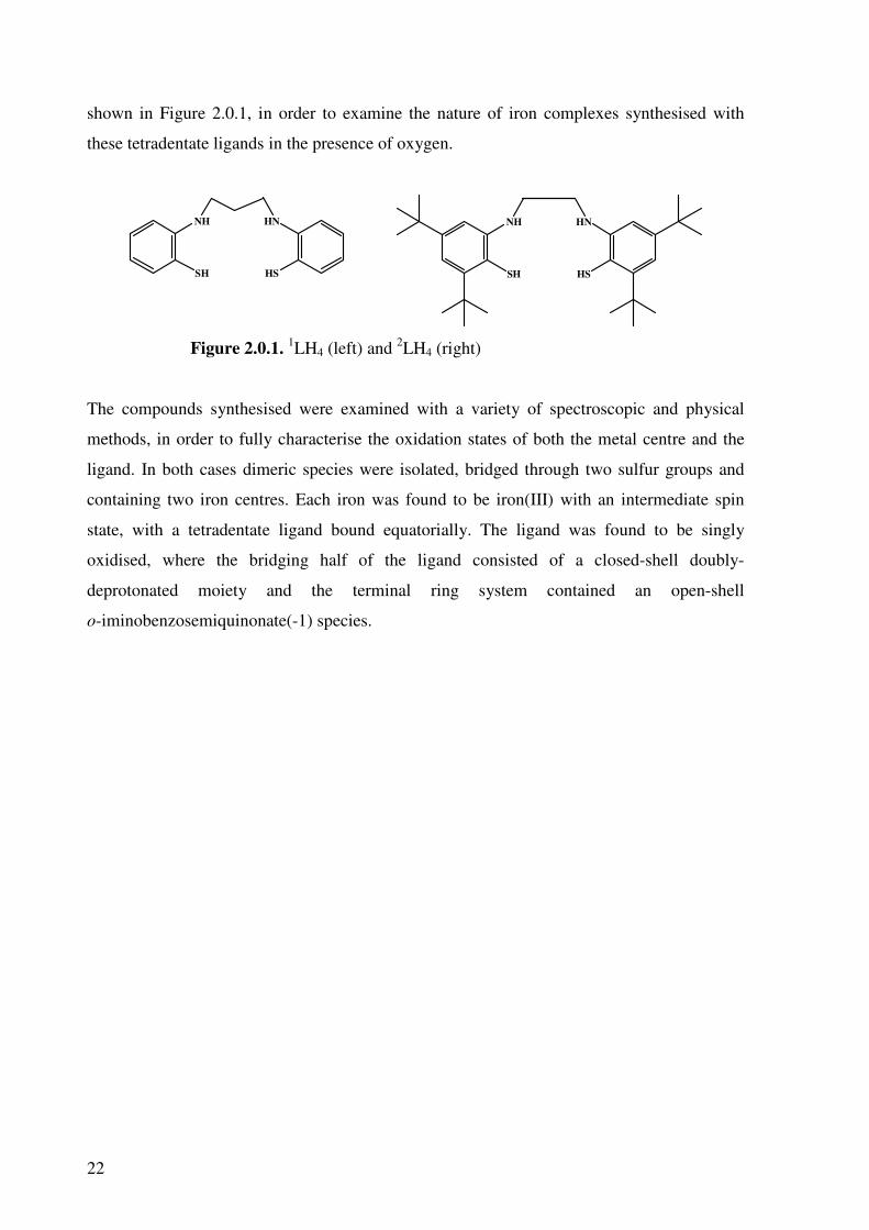
22
shown in Figure 2.0.1, in order to examine the nature of iron complexes synthesised with
these tetradentate ligands in the presence of oxygen.
NH
SH
HN
HS
NH
SH
HN
HS
Figure 2.0.1. 1LH4 (left) and 2LH4 (right)
The compounds synthesised were examined with a variety of spectroscopic and physical
methods, in order to fully characterise the oxidation states of both the metal centre and the
ligand. In both cases dimeric species were isolated, bridged through two sulfur groups and
containing two iron centres. Each iron was found to be iron(III) with an intermediate spin
state, with a tetradentate ligand bound equatorially. The ligand was found to be singly
oxidised, where the bridging half of the ligand consisted of a closed-shell doubly-
deprotonated moiety and the terminal ring system contained an open-shell
o-iminobenzosemiquinonate(-1) species.

23
2.1. [Fe(1L•)]2 (1)
Synthesis
The ligand 1,3-propanediamine-N,N’-bis-(2-benzenethiol) was dissolved in dry acetonitrile
and one equivalent of solid iron(II) bromide added under an argon blanket. Four equivalents
of distilled triethylamine were added and the solution stirred for a further two hours under an
inert atmosphere. A yellow crystalline material formed, which was filtered in the presence of
air. Upon exposure to air the yellow material turned black, and the product was washed and
isolated. Single crystals of 1 suitable for X-Ray crystallography were grown from the slow
evaporation of a CH2Cl2/hexane (2:1) solution of 1 under argon.
Crystal structure determination of 1
Crystals of 1 were analysed using single crystal X-ray diffraction and the resulting structure is
shown in Figure 2.1.1. Selected bond lengths are presented in Table 2.1.1.
Figure 2.1.1. Thermal ellipsoid plot of 1 (50% probability).
S(19)
C(2) C(3)
C(4)
C(5) C(6)
C(7)
N(8)
C(9)
C(10)
Fe(1)
N(12)
C(13)
C(14)
C(15)
C(16)
C(17) S(1)
C(11)
Fe(2)
C(18)
S(20)
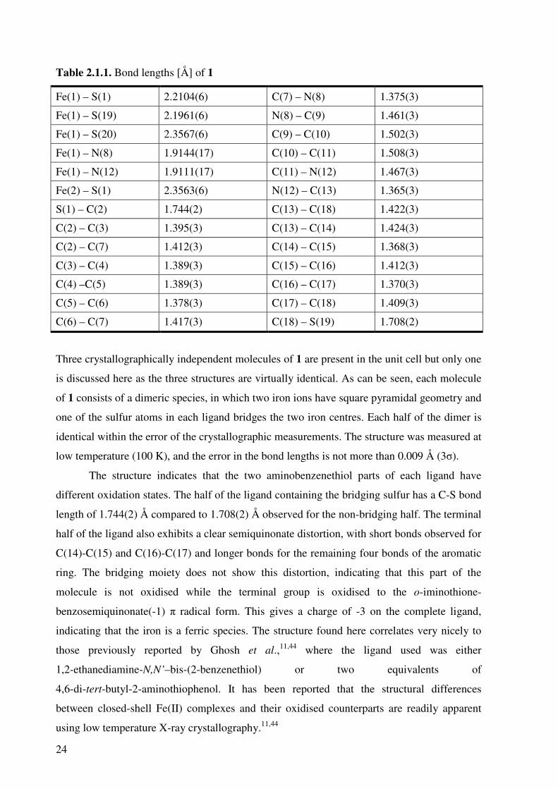
24
Table 2.1.1. Bond lengths [Å] of 1
Fe(1) – S(1) 2.2104(6) C(7) – N(8) 1.375(3)
Fe(1) – S(19) 2.1961(6) N(8) – C(9) 1.461(3)
Fe(1) – S(20) 2.3567(6) C(9) – C(10) 1.502(3)
Fe(1) – N(8) 1.9144(17) C(10) – C(11) 1.508(3)
Fe(1) – N(12) 1.9111(17) C(11) – N(12) 1.467(3)
Fe(2) – S(1) 2.3563(6) N(12) – C(13) 1.365(3)
S(1) – C(2) 1.744(2) C(13) – C(18) 1.422(3)
C(2) – C(3) 1.395(3) C(13) – C(14) 1.424(3)
C(2) – C(7) 1.412(3) C(14) – C(15) 1.368(3)
C(3) – C(4) 1.389(3) C(15) – C(16) 1.412(3)
C(4) –C(5) 1.389(3) C(16) – C(17) 1.370(3)
C(5) – C(6) 1.378(3) C(17) – C(18) 1.409(3)
C(6) – C(7) 1.417(3) C(18) – S(19) 1.708(2)
Three crystallographically independent molecules of 1 are present in the unit cell but only one
is discussed here as the three structures are virtually identical. As can be seen, each molecule
of 1 consists of a dimeric species, in which two iron ions have square pyramidal geometry and
one of the sulfur atoms in each ligand bridges the two iron centres. Each half of the dimer is
identical within the error of the crystallographic measurements. The structure was measured at
low temperature (100 K), and the error in the bond lengths is not more than 0.009 Å (3σ).
The structure indicates that the two aminobenzenethiol parts of each ligand have
different oxidation states. The half of the ligand containing the bridging sulfur has a C-S bond
length of 1.744(2) Å compared to 1.708(2) Å observed for the non-bridging half. The terminal
half of the ligand also exhibits a clear semiquinonate distortion, with short bonds observed for
C(14)-C(15) and C(16)-C(17) and longer bonds for the remaining four bonds of the aromatic
ring. The bridging moiety does not show this distortion, indicating that this part of the
molecule is not oxidised while the terminal group is oxidised to the o-iminothione-
benzosemiquinonate(-1) π radical form. This gives a charge of -3 on the complete ligand,
indicating that the iron is a ferric species. The structure found here correlates very nicely to
those previously reported by Ghosh et al.,11,44 where the ligand used was either
1,2-ethanediamine-N,N’–bis-(2-benzenethiol) or two equivalents of
4,6-di-tert-butyl-2-aminothiophenol. It has been reported that the structural differences
between closed-shell Fe(II) complexes and their oxidised counterparts are readily apparent
using low temperature X-ray crystallography.11,44

25
Electronic absorption spectroscopy
The UV-Vis spectrum measured for 1 in dichloromethane is shown in Figure 2.1.2. The
spectrum is dominated by a large band it 579 nm, which has an extinction coefficient of
13,800 M-1 cm-1. The spectrum exhibited is very similar to that observed by Ghosh et al. for
the previously mentioned compounds.11 The large band at 579 nm is probably a spin- and
dipole-allowed ligand-to-metal charge-transfer (LMCT) band. This band has also been
examined for iron dimer complexes with N-phenyl-1,2-benzenediamine ligands,37 and similar
bands (albeit at lower energy) are observed for nickel(II), palladium(II) and platinum(II)
complexes containing two o-aminothiophenol ligands, where one is in the closed-shell
dianionic oxidation state and the other is an oxidised semi-quinonate π radical.69
It has been hypothesised by Chlopek et al.38 for Fe(III) dimers containing N-phenyl-
1,2-benzenediamine ligands that the lower energy, lower intensity bands in the shoulder of the
major band consist of ligand-to-ligand intervalence charge-transfer bands (LLIVCT) of the
type [LML•] � [L•ML], where L• is the oxidised semi-quinonate π radical half of the ligand
and L denotes the aromatic dianionic portion. This may also be the case for complex 1.
400 600 800 1000 1200 1400
0.0
0.2
0.4
0.6
0.8
1.0
1.2
1.4
εε εε / 10
4 M
-1 c
m-1
λλλλ / nm
Figure 2.1.2. UV-vis spectrum of 1 recorded in
dichloromethane.
Mössbauer spectroscopy
The zero-field Mössbauer spectrum measured at 80 K and an applied-field measurement of
the solid sample at 7 T and 4 K of 1 are shown in Figure 2.1.4. The zero-field measurement
gives one major doublet with an isomer shift of 0.24 mm s-1 and a quadrupole splitting of 2.51
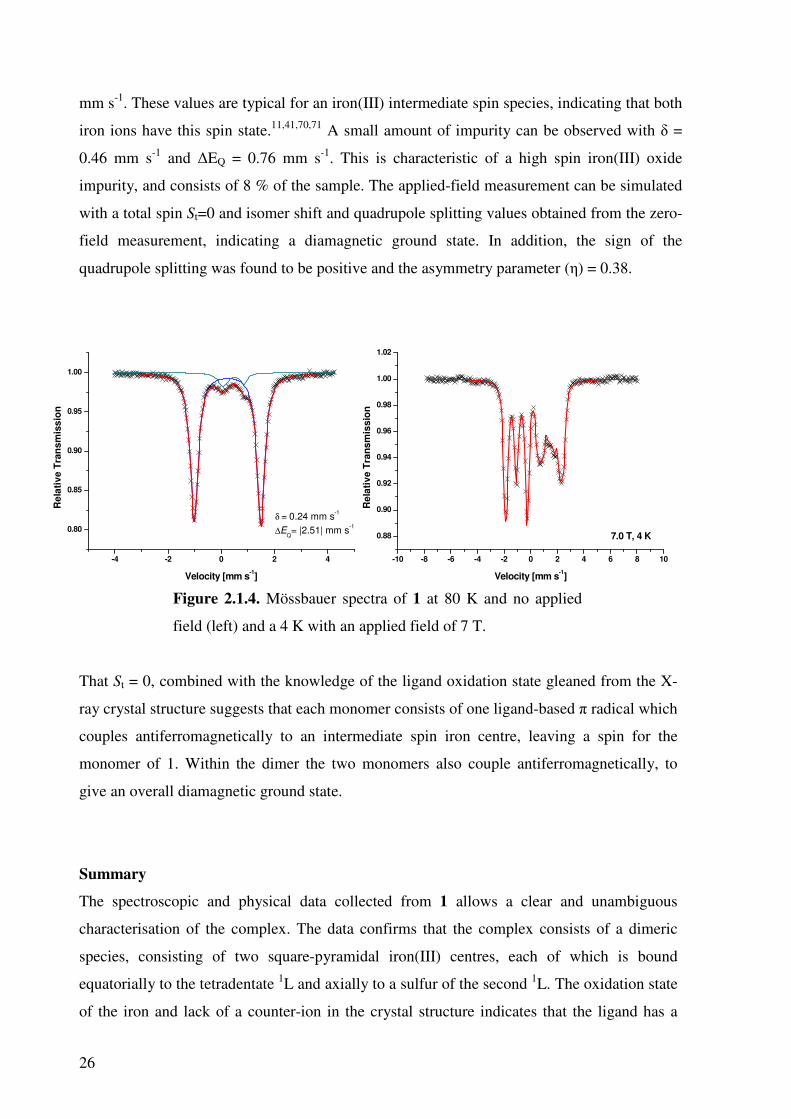
26
mm s-1. These values are typical for an iron(III) intermediate spin species, indicating that both
iron ions have this spin state.11,41,70,71 A small amount of impurity can be observed with δ =
0.46 mm s-1 and ∆EQ = 0.76 mm s-1. This is characteristic of a high spin iron(III) oxide
impurity, and consists of 8 % of the sample. The applied-field measurement can be simulated
with a total spin St=0 and isomer shift and quadrupole splitting values obtained from the zero-
field measurement, indicating a diamagnetic ground state. In addition, the sign of the
quadrupole splitting was found to be positive and the asymmetry parameter (η) = 0.38.
Figure 2.1.4. Mössbauer spectra of 1 at 80 K and no applied
field (left) and a 4 K with an applied field of 7 T.
That St = 0, combined with the knowledge of the ligand oxidation state gleaned from the X-
ray crystal structure suggests that each monomer consists of one ligand-based π radical which
couples antiferromagnetically to an intermediate spin iron centre, leaving a spin for the
monomer of 1. Within the dimer the two monomers also couple antiferromagnetically, to
give an overall diamagnetic ground state.
Summary
The spectroscopic and physical data collected from 1 allows a clear and unambiguous
characterisation of the complex. The data confirms that the complex consists of a dimeric
species, consisting of two square-pyramidal iron(III) centres, each of which is bound
equatorially to the tetradentate 1L and axially to a sulfur of the second 1L. The oxidation state
of the iron and lack of a counter-ion in the crystal structure indicates that the ligand has a
-4 -2 0 2 4
0.80
0.85
0.90
0.95
1.00
δ = 0.24 mm s-1
∆EQ= |2.51| mm s
-1
Re
lati
ve T
ran
sm
iss
ion
Velocity [mm s-1]
-10 -8 -6 -4 -2 0 2 4 6 8 10
0.88
0.90
0.92
0.94
0.96
0.98
1.00
1.02
7.0 T, 4 K
Re
lati
ve
Tra
ns
mis
sio
n
Velocity [mm s-1]
27
charge of -3. Thus 1L must be oxidised by one equivalent, giving a π radical species. There is
evidence for this in the X-ray crystal structure, in that the non-bridging rings both show
extensive semi-quinoidal distortion, with a pattern of four long and two short carbon-carbon
bonds. The bridging group also shows a non-quinoidal distortion, which has been observed in
the bridging moiety of other similar dimeric complexes.11
The electronic absorption spectrum of 1 shows an intense band at 579 nm, which
corresponds to previously observed bands as being a LMCT band. This band has been
detected in iron dimer compounds containing four 1,2-benzenediamine based ligands, where
two ligands are closed-shell aromatic dianions and the others are oxidised and contain open-
shell π radicals.
Mössbauer spectroscopy gives one doublet, demonstrating that the two iron centres
have the same oxidation and spin states. The isomer shift of 0.24 mm s-1 and a quadrupole
splitting of 2.51 mm s-1 are classic values for an intermediate-spin iron(III) system.11,41,70,71
The applied field Mössbauer measurement confirms the sign of the quadrupole splitting as
positive, and also shows the complex to have a diamagnetic (St=0) ground state. In order to
achieve a diamagnetic complex, the two ligand-based radicals must couple
antiferromagnetically to the iron centres, which then couple antiferromagnetically to each
other through the bridging sulfur moieties.
Complex 1 is thus characterised as a dimer species containing a two-iron two-sulfur
core. Each iron nucleus is an intermediate-spin iron(III) species. Each iron(III) centre couples
antiferromagnetically to a ligand-based π radical, which is located on the terminal ring of the
ligand. The iron(III) nuclei also couple antiferromagnetically with each other, giving a
diamagnetic ground state.
28
2.2. [Fe(2L•)]2 (2)
Synthesis
The ligand 2L was dissolved in dry degassed acetonitrile with five molar equivalents of
triethylamine. One equivalent of solid FeBr2 was added to the stirring solution under an
argon blanket. The solution was stirred and 1 mL of air bubbled through the solution every 5-
10 minutes. The solution turned purple immediately upon the addition of air, and after one
hour a grey precipitate could be removed by filtration. This was then dissolved in distilled
diethyl ether and filtered before removal of the volatiles under vacuum. This step was
repeated until a Mössbauer clean sample of the product was obtained. Single crystals suitable
for X-ray crystallography were grown in 2002 by Jos Wilting in this group by dissolving the
product in a CH2Cl2/n-hexane 3:2 solution and allowing the solution to slowly evaporate.
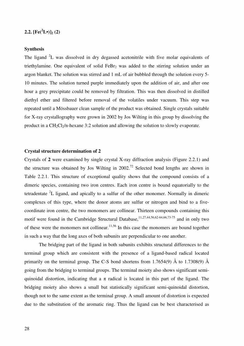
Crystal structure determination of 2
Crystals of 2 were examined by single crystal X-ray diffraction analysis (Figure 2.2.1) and
the structure was obtained by Jos Wilting in 2002.72 Selected bond lengths are shown in
Table 2.2.1. This structure of exceptional quality shows that the compound consists of a
dimeric species, containing two iron centres. Each iron centre is bound equatorially to the
tetradentate 2L ligand, and apically to a sulfur of the other monomer. Normally in dimeric
complexes of this type, where the donor atoms are sulfur or nitrogen and bind to a five-
coordinate iron centre, the two monomers are collinear. Thirteen compounds containing this
motif were found in the Cambridge Structural Database,11,27,44,56,62-64,66,73-75 and in only two
of these were the monomers not collinear.11,56 In this case the monomers are bound together
in such a way that the long axes of both subunits are perpendicular to one another.
The bridging part of the ligand in both subunits exhibits structural differences to the
terminal group which are consistent with the presence of a ligand-based radical located
primarily on the terminal group. The C-S bond shortens from 1.7654(9) Å to 1.7308(9) Å
going from the bridging to terminal groups. The terminal moiety also shows significant semi-
quinoidal distortion, indicating that a π radical is located in this part of the ligand. The
bridging moiety also shows a small but statistically significant semi-quinoidal distortion,
though not to the same extent as the terminal group. A small amount of distortion is expected
due to the substitution of the aromatic ring. Thus the ligand can be best characterised as

29
containing one π radical located in the terminal ring and a closed-shell aromatic system in the
bridging ring. This gives a ligand with an overall charge of -3.
There is considerable distortion within the plane of the ligand. The whole ligand is
bent about the iron centre. The angle between the two planes formed by the ligand is found to
be 34.7°. This is not observed with the similar compounds [FeL]2 where L = 1,2-
ethanediamine-N,N’-bis-(2-benzenethiol)11 or glyoxal-bis-(2-mercaptoanil).56 However this
type of distortion is detected in [FeL2]2, where L is 4,6-di-tert-butyl-2-aminothiophenol.44
Therefore this distortion is thought to arise out of steric hindrance between the bulky tert-
butyl groups of the ligand and the other subunit of the dimer.
To summarise, the crystal structure indicates that solid compound 2 consists of a
dimeric species, where each subunit is made up of an iron(III) bound equatorially to the
tetradentate ligand 2L. The ligand is one electron oxidised, giving a π radical located in the
terminal group while the other half of the ligand consists of a closed-shell aromatic moiety.
Table 2.2.1. Bond lengths [Å] of 2
Fe(1) – S(1) 2.1987(4) C(7) – N(8) 1.3648(12)
Fe(1) – S(18) 2.1836(3) N(8) – C(9) 1.4574(12)
Fe(1) – S(19) 2.3195(3) C(9) – C(10) 1.5265(13)
Fe(1) – N(8) 1.8581(8) C(10) – N(11) 1.4621 (12)
Fe(1) – N(11) 1.8510(8) N(12) – C(13) 1.3597 (11)
Fe(2) – S(1) 2.3195(3) C(12) – C(17) 1.4263(12)
S(1) – C(2) 1.7654(9) C(12) – C(13) 1.4161(13)
C(2) – C(3) 1.4170(13) C(13) – C(14) 1.3714(13)
C(2) – C(7) 1.4198(12) C(14) – C(15) 1.4224(13)
C(3) – C(4) 1.3903(13) C(15) – C(16) 1.3856(14)
C(4) –C(5) 1.4091(13) C(16) – C(17) 1.4280(13)
C(5) – C(6) 1.3833(13) C(17) – S(18) 1.7308(9)
C(6) – C(7) 1.4138(12)
30
Figure 2.2.1. Thermal ellipsoid plot of 2 at a probability level
of 50%. The complete structure is shown above, and below one
subunit is picked out for clarity.
Fe(1)
Fe(2)
S(1) S(19)
S(18)
C(17) C(16)
C(15)
C(14) C(13)
C(12) N(11)
C(10) C(9)
N(8) C(7)
C(6) C(5)
C(4)
C(3) C(2)
31
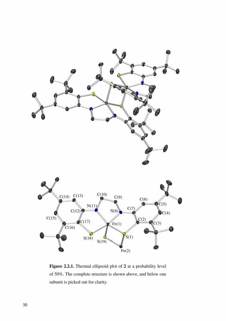
Electronic absorption spectroscopy
The electronic spectrum of 2 measured in toluene (Figure 2.2.2) is dominated by a large band
at 545 nm, which has an extinction coefficient of 1.39×10⁻⁴ M-1 cm-1. The features of this
spectrum are very similar to those observed for 1, and therefore we assign the large band to a
spin- and dipole-allowed LMCT band. This band has been observed previously in an iron
complex containing N-phenyl-1,2-benzenediamine ligands37 and in several dimeric
complexes containing aminobenzenethiol type ligands11 where the ligands are assigned as
containing a π radical in the terminal group and an aromatic closed-shell system in the
bridging group. As previously noted for 1, it has been suggested previously that the low
energy shoulders observed in the UV-vis spectrum for Fe(III) dimers containing N-phenyl-
1,2-benzenediamine ligands consist of intervalence ligand-to-ligand charge transfer bands.
These low energy bands are observed here also, and may arise from this transition.38
400 600 800 1000 1200 1400 1600 1800 2000
0.0
0.5
1.0
1.5
2.0
εε εε / 1
04 M
-1 c
m-1
λλλλ / nm
Figure 2.2.2. UV-vis spectrum of 2 recorded in toluene.
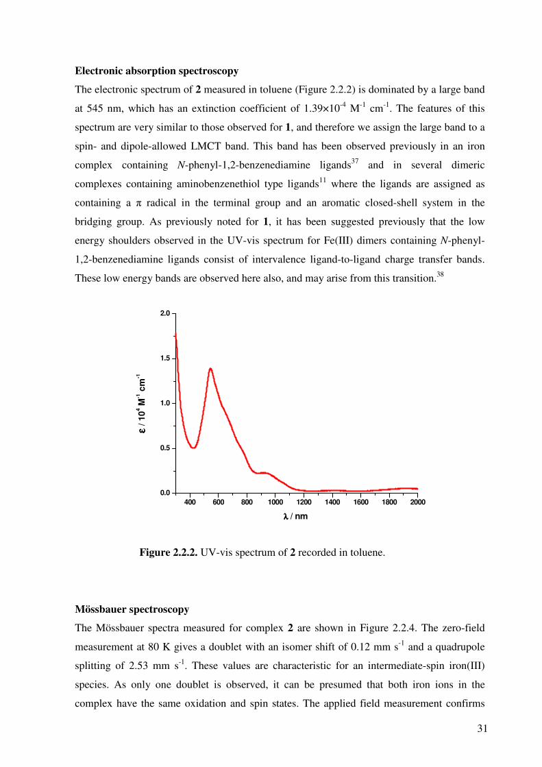
Mössbauer spectroscopy
The Mössbauer spectra measured for complex 2 are shown in Figure 2.2.4. The zero-field
measurement at 80 K gives a doublet with an isomer shift of 0.12 mm s-1 and a quadrupole
splitting of 2.53 mm s-1. These values are characteristic for an intermediate-spin iron(III)
species. As only one doublet is observed, it can be presumed that both iron ions in the
complex have the same oxidation and spin states. The applied field measurement confirms
32
that the value for ∆EQ is positive. The spectrum can be simulated by taking the values
discussed above with a spin state for the molecule St = 0. The lack of splitting due to an
internal field signifies that the compound has a diamagnetic ground state. Thus the
ligand-based radicals must couple antiferromagnetically to the iron centre, and the iron
centres to each other to give St = 0.
-4 -2 0 2 4
0.86
0.88
0.90
0.92
0.94
0.96
0.98
1.00
Re
lati
ve T
ran
sm
issio
n
Velocity [mm s-1]
-4 -2 0 2 4
0.92
0.94
0.96
0.98
1.00
Re
lati
ve T
ran
sm
issio
n
Velocity [mm s-1]
Figure 2.2.4. Mössbauer spectra of solid 2 with no external
field and at 80 K (left), and with an applied field of 7 T at 4.2 K
(right).
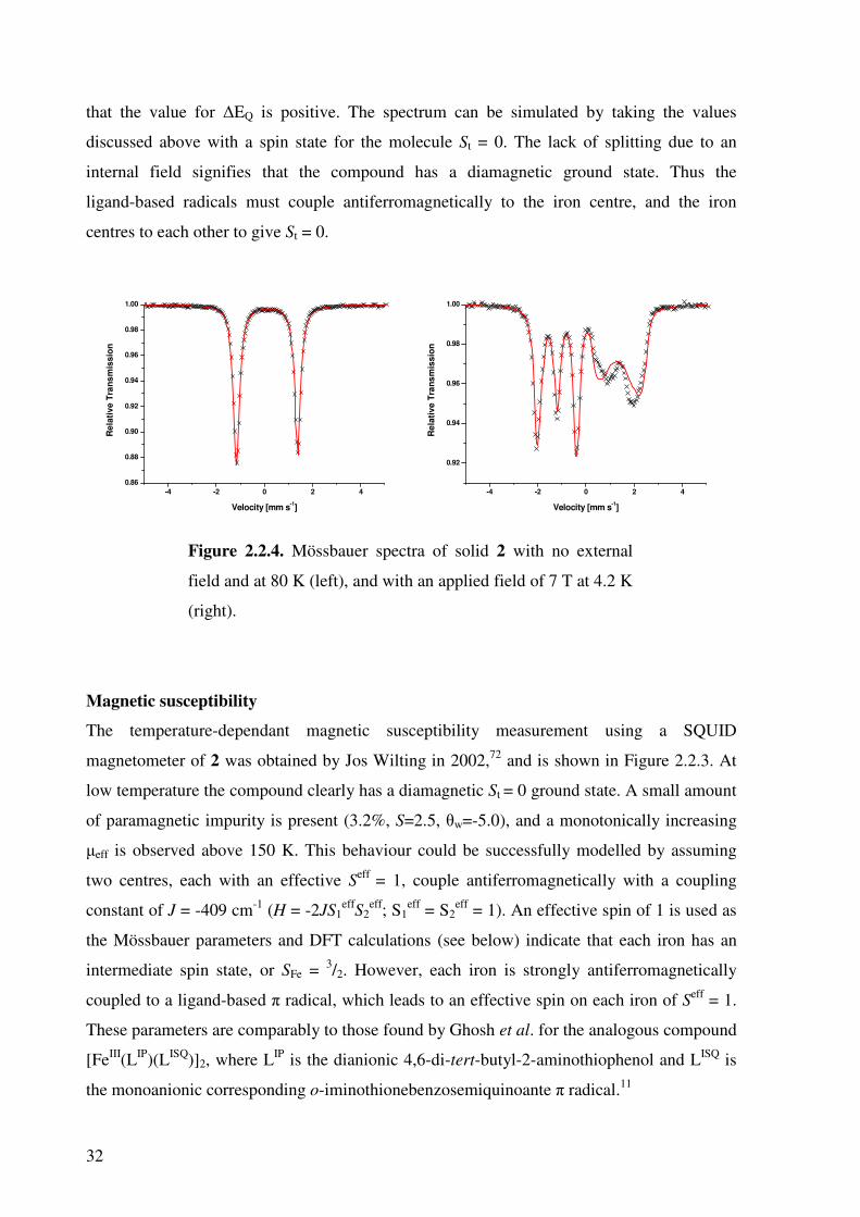
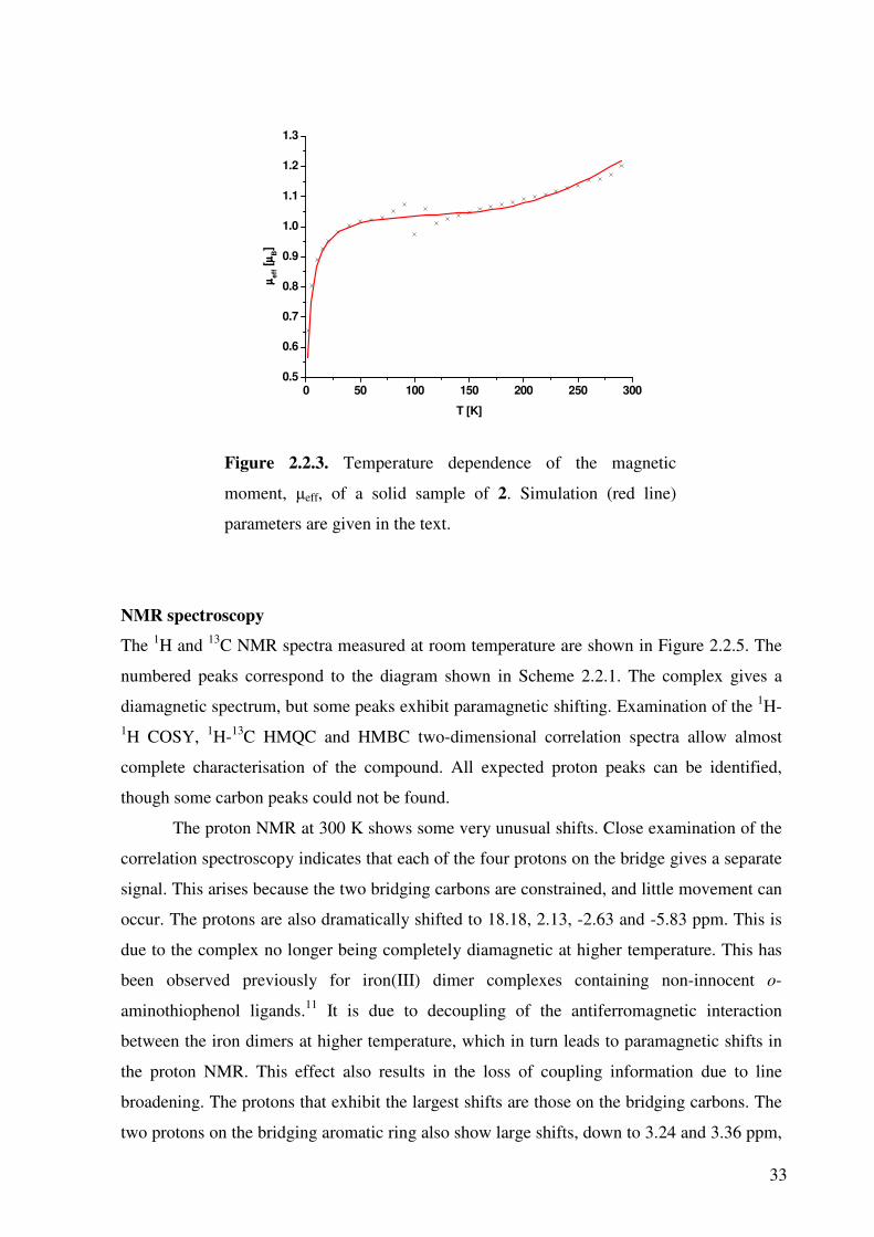
Magnetic susceptibility
The temperature-dependant magnetic susceptibility measurement using a SQUID
magnetometer of 2 was obtained by Jos Wilting in 2002,72 and is shown in Figure 2.2.3. At
low temperature the compound clearly has a diamagnetic St = 0 ground state. A small amount
of paramagnetic impurity is present (3.2%, S=2.5, θw=-5.0), and a monotonically increasing
µeff is observed above 150 K. This behaviour could be successfully modelled by assuming
two centres, each with an effective Seff
= 1, couple antiferromagnetically with a coupling
constant of J = -409 cm-1 (H = -2JS1eff
S2eff; S1
eff = S2eff = 1). An effective spin of 1 is used as
the Mössbauer parameters and DFT calculations (see below) indicate that each iron has an
intermediate spin state, or SFe = 3/2. However, each iron is strongly antiferromagnetically
coupled to a ligand-based π radical, which leads to an effective spin on each iron of Seff = 1.
These parameters are comparably to those found by Ghosh et al. for the analogous compound
[FeIII(LIP)(LISQ)]2, where LIP is the dianionic 4,6-di-tert-butyl-2-aminothiophenol and LISQ is
the monoanionic corresponding o-iminothionebenzosemiquinoante π radical.11
33
0 50 100 150 200 250 3000.5
0.6
0.7
0.8
0.9
1.0
1.1
1.2
1.3
µµ µµeff [
µµ µµB]
T [K]
Figure 2.2.3. Temperature dependence of the magnetic
moment, µeff, of a solid sample of 2. Simulation (red line)
parameters are given in the text.
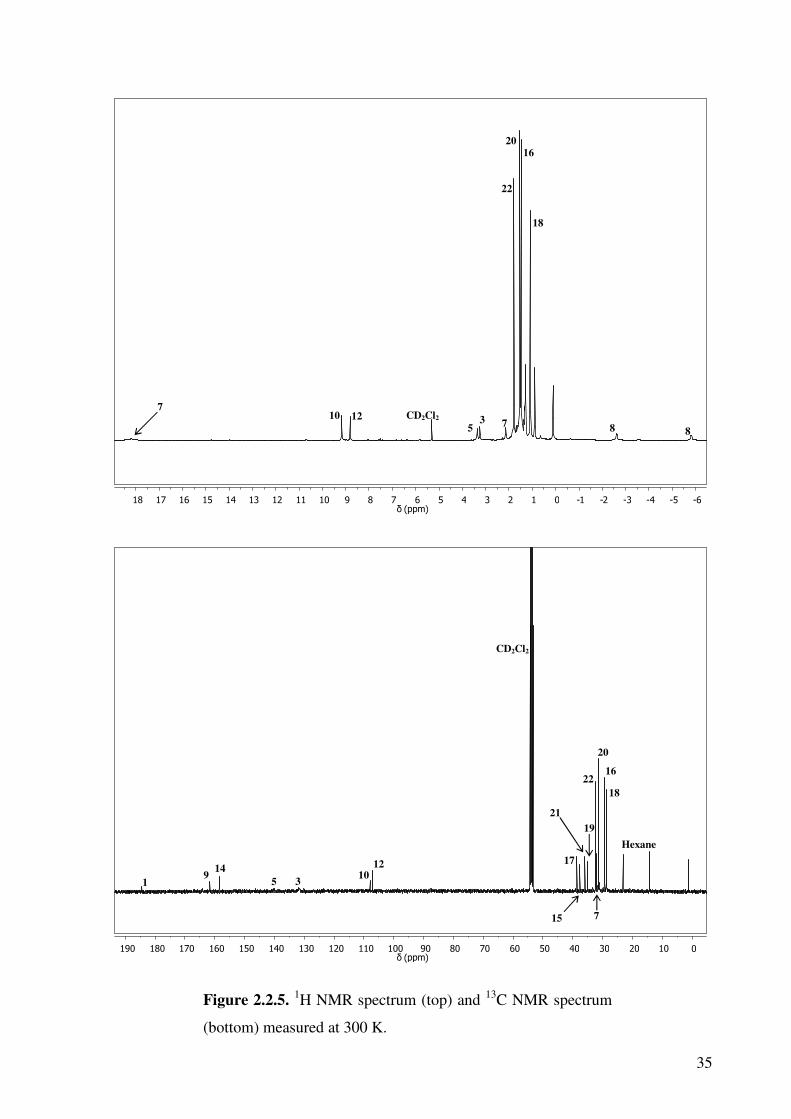
NMR spectroscopy
The 1H and 13C NMR spectra measured at room temperature are shown in Figure 2.2.5. The
numbered peaks correspond to the diagram shown in Scheme 2.2.1. The complex gives a
diamagnetic spectrum, but some peaks exhibit paramagnetic shifting. Examination of the 1H-1H COSY, 1H-13C HMQC and HMBC two-dimensional correlation spectra allow almost
complete characterisation of the compound. All expected proton peaks can be identified,
though some carbon peaks could not be found.
The proton NMR at 300 K shows some very unusual shifts. Close examination of the
correlation spectroscopy indicates that each of the four protons on the bridge gives a separate
signal. This arises because the two bridging carbons are constrained, and little movement can
occur. The protons are also dramatically shifted to 18.18, 2.13, -2.63 and -5.83 ppm. This is
due to the complex no longer being completely diamagnetic at higher temperature. This has
been observed previously for iron(III) dimer complexes containing non-innocent o-
aminothiophenol ligands.11 It is due to decoupling of the antiferromagnetic interaction
between the iron dimers at higher temperature, which in turn leads to paramagnetic shifts in
the proton NMR. This effect also results in the loss of coupling information due to line
broadening. The protons that exhibit the largest shifts are those on the bridging carbons. The
two protons on the bridging aromatic ring also show large shifts, down to 3.24 and 3.36 ppm,

34
due to the proximity to the two iron centres. The protons on the terminal ring are slightly
shifted but not nearly to the same extent. This part of the molecule is insulated from the
second iron centre.
N
S
N
S
Fe
N
S
N
S
Fe
12
3
4
5
6
78
910
11
12
1314
2122
19
20
15
16
1718
Scheme 2.2.1. Numbering of the carbon and hydrogen atoms of 2.
35
Figure 2.2.5. 1H NMR spectrum (top) and 13C NMR spectrum
(bottom) measured at 300 K.
010203040 506070 8090100 110 120 130140 150 160170 180 190δ ( ppm )
1 9
14
5 3 10
12 17
19
21
15
22
20
16
18
CD2Cl2
Hexane
7
- 6 - 5 - 4 - 3 - 2- 1 012 345 6 7 8 91011 1213 14151617 18δ ( ppm )
7 10
12
5 3 7
22
20 16
18
8 8
CD2Cl2

36
Table 2.2.2. 1H and 13C NMR chemical shifts (ppm) for 2 in CD2Cl2 at 300 K
Atom 1 2 3 4 5 6
1H ― ― s, 3.24 ― s, 3.36 ― 13C 184.48 n/oa 131.89 158.51 140.52 n/oa
Atom 7 8 9 10
1H s, 18.18; s, 2.13 d, -2.63; s, -5.83 ― s, 9.17 13C n/oa 31.98 161.64 107.91
Atom 11 12 13 14 15 16
1H ― s, 8.80 ― ― ― s, 1.48 13C n/oa 107.17 n/oa 158.51 37.69 29.38
Atom 17 18 19 20 21 22
1H ― s, 1.09 ― s, 1.54 ― s, 1.80 13C 38.59 28.73 35.02 31.46 36.08 32.43
a) n/o marked bands are not observed.
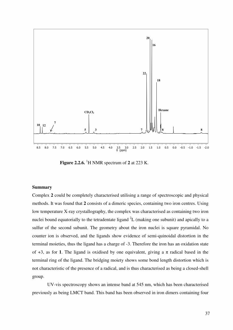
The NMR spectra measured at low temperature (Figure 2.2.6) support this explanantion, as
all of the paramagnetically shifted peaks move towards the diamagnetic region. The protons
on carbons 5 and 3 have moved from 3.36 and 3.24 ppm to 5.51 and 5.01 ppm respectively.
Most dramatically, the proton signal on carbon 7 has shifted from 18.18 to 7.78 ppm. While
still unusual, this value falls much closer to the expected value of ~3-4 ppm.
37
Figure 2.2.6. 1H NMR spectrum of 2 at 223 K.
Summary
Complex 2 could be completely characterised utilising a range of spectroscopic and physical
methods. It was found that 2 consists of a dimeric species, containing two iron centres. Using
low temperature X-ray crystallography, the complex was characterised as containing two iron
nuclei bound equatorially to the tetradentate ligand 2L (making one subunit) and apically to a
sulfur of the second subunit. The geometry about the iron nuclei is square pyramidal. No
counter ion is observed, and the ligands show evidence of semi-quinoidal distortion in the
terminal moieties, thus the ligand has a charge of -3. Therefore the iron has an oxidation state
of +3, as for 1. The ligand is oxidised by one equivalent, giving a π radical based in the
terminal ring of the ligand. The bridging moiety shows some bond length distortion which is
not characteristic of the presence of a radical, and is thus characterised as being a closed-shell
group.
UV-vis spectroscopy shows an intense band at 545 nm, which has been characterised
previously as being LMCT band. This band has been observed in iron dimers containing four
- 2 . 0 - 1 . 5 - 1 . 0 - 0 . 5 0 .0 0.5 1 .0 1.5 2.02 .53. 0 3 . 54 . 0 4 . 55 . 05 . 5 6. 06. 5 7. 07. 5 8. 0 8. 5 δ ( ppm )
7 10
5
12
3
22
20
16
18
8 8 7
CD2Cl2
Hexane
38
1,2-benzenediamine based ligands, and also in square planar complexes of group 10 metals
where the oxidation states of the two aminothiophenol based ligands differ by one electron.69
Mössbauer spectroscopy shows one quadrupole doublet, which has an isomer shift of
0.12 mm s-1 and ∆EQ = 2.53 mm s-1. These values correspond nicely to those observed
previously for intermediate spin iron(III) species. The applied field measurement establishes
that the complex has a singlet ground state, shown by the lack of splitting due to an internal
field. The diamagnetic ground state arises through extensive antiferromagnetic coupling. The
ligand-based π-radicals couple to the coordinated intermediate-spin iron nuclei, which leaves
each monomer with S=1. The spin present on each monomer in turn couples in an
antiferromagnetic fashion, giving rise to a singlet ground state.
Proton NMR spectroscopy provides a room temperature spectrum in which some
peaks are paramagnetically shifted. This could arise though several mechanisms, including
exchange of dimer subunits. It is likely however that this arises due to decoupling of the spin
of the monomers at higher temperatures. The coupling between the two iron centres is much
weaker than that between the radicals and iron(III) nuclei. Thus at higher temperature, higher
spin states are populated. This has been observed previously for dimers of this type.11 The
spectrum measured at low temperature confirms this, as the shifted signals move closer to a
diamagnetic spectrum.
Complex 2 has been fully characterised as a dimer consisting of two square-pyramidal
intermediate-spin iron(III) centres bound to two 2L molecules, both of which contain one
ligand π-radical. The monomers bind through two bridging sulfurs, each of which is bound to
both iron centres. The terminal ring system of each ligand contains a radical, both of which
couple antiferromagnetically to the iron centres, and the two iron nuclei couple
antiferromagnetically through the bridging sulfurs.
2.3. DFT calculations of 1 and 2
Further study of complexes 1 and 2 was undertaken using density functional theory (DFT)
calculations, utilising the Orca software package.76 Full details of the calculation methods are
provided in chapter 7. The Orca package allows the calculation of broken symmetry
solutions, where unpaired electron density can be found on various parts of the compound in
question. This is very useful when a ligand-based radical is suspected, as Orca can calculate
the lowest energy electronic state for the compound.

39
BS-DFT solutions were calculated for both 1 and 2 (where the tertiary butyl groups
were truncated to methyl groups), as well as unrestricted Kohn-Sham (UKS) solutions for
comparison. In both cases the UKS calculation converged on solutions that were higher in
energy (by 1.9 kcal mol-1 for 1 and 1.7 kcal mol-1 for 2). This validates the broken symmetry
solution in both cases, though the values are approaching the accuracy limit of DFT. The
calculated geometrical parameters from geometry optimisation were comparable to those
obtained from the X-ray crystal structure. Further corroboration for the broken symmetry
solution was obtained from the calculated Mössbauer parameters. Figure 2.3.1 shows the
calculated structure of 1, and the calculated and experimental bond lengths are presented in
Table 2.3.1.
Figure 2.3.1. Diagram showing numbering of the atoms in 1
and for reference to Table 3.3.1.
The calculated bond lengths compare quite well to those observed in the X-ray crystal
structures. Some deviation is observed in the metal to ligand bonds, but a lengthening of
these bonds is expected when the B3LYP functional is used.77 The bond lengths between the
monomers deviate by 0.2 Å, which is considerably different even when allowing for the
lengthening due to the B3LYP functional. However, the bond lengths through the ligand are
very nicely reproduced, and clearly show the semi-quinoidal distortion in the terminal
aromatic group.
C(15)
C(14)
S(1) S(19)
C(2) C(3)
C(4)
C(5) C(6)
C(7) N(8)
C(9) C(10) C(11)
C(16) N(12)
C(13)
Fe(1) C(17) C(18)
S(20)
Fe(2)

40
Table 2.3.1. Comparison of bond lengths [Å] between the geometry optimisation of the
BS(2,2) DFT calculation and the experimental values obtained from single crystal X-ray
measurements for 1.
Experimental values BS(2,2) calculation
Fe(1) – N(8) 1.9144(17) 1.922
Fe(1) – N(12) 1.9111(17) 1.970
Fe(1) – S(1) 2.2104(6) 2.284
Fe(1) – S(19) 2.1961(6) 2.275
Fe(1) – S(20) 2.3567(6) 2.574
Fe(2) – S(1) 2.3563(6) 2.574
S(1) – C(2) 1.744(2) 1.766
C(2) – C(3) 1.395(3) 1.398
C(2) – C(7) 1.412(3) 1.421
C(3) – C(4) 1.389(3) 1.396
C(4) – C(5) 1.389(3) 1.402
C(5) – C(6) 1.378(3) 1.394
C(6) – C(7) 1.417(3) 1.421
C(7) – N(8) 1.375(3) 1.383
N(8) – C(9) 1.461(3) 1.458
C(9) – C(10) 1.502(3) 1.522
C(10) – C(11) 1.508(3) 1.521
C(11) – N(12) 1.467(3) 1.462
N(12) – C(13) 1.365(3) 1.354
C(13) – C(18) 1.422(3) 1.443
C(13) – C(14) 1.424(3) 1.434
C(14) – C(15) 1.368(3) 1.380
C(15) – C(16) 1.412(3) 1.419
C(16) – C(17) 1.370(3) 1.383
C(17) – C(18) 1.409(3) 1.414
C(18) – S(19) 1.708(2) 1.722

41
The calculated structure for 2 is shown in Figure 2.3.2, and the calculated bond lengths
compared with the X-ray crystal structure in Table 2.3.2.
Figure 2.3.2. Diagram showing numbering of the atoms in
truncated 2 and for reference to Table 3.3.1.
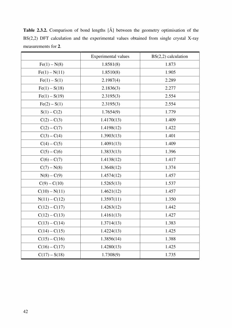
The calculated bond lengths are in good agreement with the measured bond lengths of 2. The
metal-ligand bond lengths are as expected elongated in the calculation. The bond distances
between the two subunits show very large elongation, from 2.3195(3) Å to 2.554 Å.
However, the bond lengths within the two ligands are very nicely reproduced to within 0.02
Å, and the semi-quinoidal distortion of the terminal groups observed by X-ray
crystallography is also duplicated.
The calculated broken symmetry solution can be corroborated through the calculation
of the Mössbauer parameters.78 Comparison of the calculated values for the isomer shift and
quadrupole splitting with the spectroscopically obtained parameters gives a direct measure of
the validity of the calculated solution. The calculated and experimental Mössbauer
parameters are shown in Table 2.3.3.
C(15)
C(14) S(1)
C(2) C(3)
C(4) C(5)
C(6)
C(7) N(8)
C(9) C(10)
N(11) C(12) C(13)
C(16)
C(17) S(18)
Fe(1)
Fe(2) S(19)
42
Table 2.3.2. Comparison of bond lengths [Å] between the geometry optimisation of the
BS(2,2) DFT calculation and the experimental values obtained from single crystal X-ray
measurements for 2.
Experimental values BS(2,2) calculation
Fe(1) – N(8) 1.8581(8) 1.873
Fe(1) – N(11) 1.8510(8) 1.905
Fe(1) – S(1) 2.1987(4) 2.289
Fe(1) – S(18) 2.1836(3) 2.277
Fe(1) – S(19) 2.3195(3) 2.554
Fe(2) – S(1) 2.3195(3) 2.554
S(1) – C(2) 1.7654(9) 1.779
C(2) – C(3) 1.4170(13) 1.409
C(2) – C(7) 1.4198(12) 1.422
C(3) – C(4) 1.3903(13) 1.401
C(4) – C(5) 1.4091(13) 1.409
C(5) – C(6) 1.3833(13) 1.396
C(6) – C(7) 1.4138(12) 1.417
C(7) – N(8) 1.3648(12) 1.374
N(8) – C(9) 1.4574(12) 1.457
C(9) – C(10) 1.5265(13) 1.537
C(10) – N(11) 1.4621(12) 1.457
N(11) – C(12) 1.3597(11) 1.350
C(12) – C(17) 1.4263(12) 1.442
C(12) – C(13) 1.4161(13) 1.427
C(13) – C(14) 1.3714(13) 1.383
C(14) – C(15) 1.4224(13) 1.425
C(15) – C(16) 1.3856(14) 1.388
C(16) – C(17) 1.4280(13) 1.425
C(17) – S(18) 1.7308(9) 1.735
43
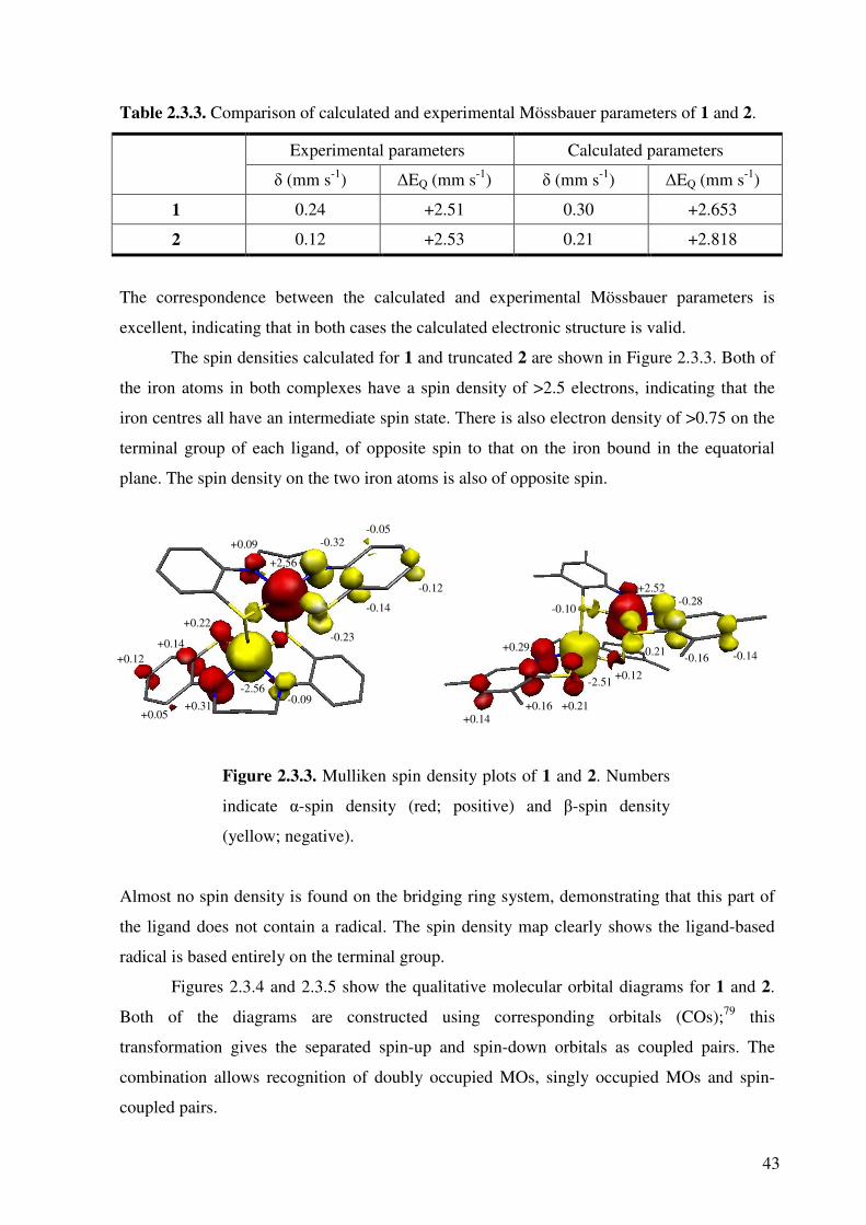
Table 2.3.3. Comparison of calculated and experimental Mössbauer parameters of 1 and 2.
Experimental parameters Calculated parameters
δ (mm s-1) ∆EQ (mm s-1) δ (mm s-1) ∆EQ (mm s-1)
1 0.24 +2.51 0.30 +2.653
2 0.12 +2.53 0.21 +2.818
The correspondence between the calculated and experimental Mössbauer parameters is
excellent, indicating that in both cases the calculated electronic structure is valid.
The spin densities calculated for 1 and truncated 2 are shown in Figure 2.3.3. Both of
the iron atoms in both complexes have a spin density of >2.5 electrons, indicating that the
iron centres all have an intermediate spin state. There is also electron density of >0.75 on the
terminal group of each ligand, of opposite spin to that on the iron bound in the equatorial
plane. The spin density on the two iron atoms is also of opposite spin.
Figure 2.3.3. Mulliken spin density plots of 1 and 2. Numbers
indicate α-spin density (red; positive) and β-spin density
(yellow; negative).
Almost no spin density is found on the bridging ring system, demonstrating that this part of
the ligand does not contain a radical. The spin density map clearly shows the ligand-based
radical is based entirely on the terminal group.
Figures 2.3.4 and 2.3.5 show the qualitative molecular orbital diagrams for 1 and 2.
Both of the diagrams are constructed using corresponding orbitals (COs);79 this
transformation gives the separated spin-up and spin-down orbitals as coupled pairs. The
combination allows recognition of doubly occupied MOs, singly occupied MOs and spin-
coupled pairs.
+2.56
-0.32 +0.09
-2.56
-0.23
-0.14
-0.12
-0.05
-0.09 +0.31 +0.05
+0.12 +0.14
+0.22
+2.52 -0.28
-0.21 -0.16 -0.14
-2.51
-0.10
+0.29
+0.21 +0.14
+0.16
+0.12
44
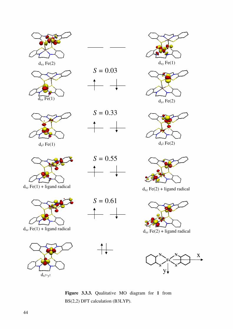
Figure 3.3.3. Qualitative MO diagram for 1 from
BS(2,2) DFT calculation (B3LYP).
S = 0.55
S = 0.33
dxz Fe(2) + ligand radical
dz2 Fe(2)
dyz Fe(2)
dxy Fe(1)
dxz Fe(2) + ligand radical
S = 0.61
S = 0.03
N
S
N
S
Fe
y
x
dx2-y2
dxz Fe(1) + ligand radical
dxz Fe(1) + ligand radical
dz2 Fe(1)
dyz Fe(1)
dxy Fe(2)
45
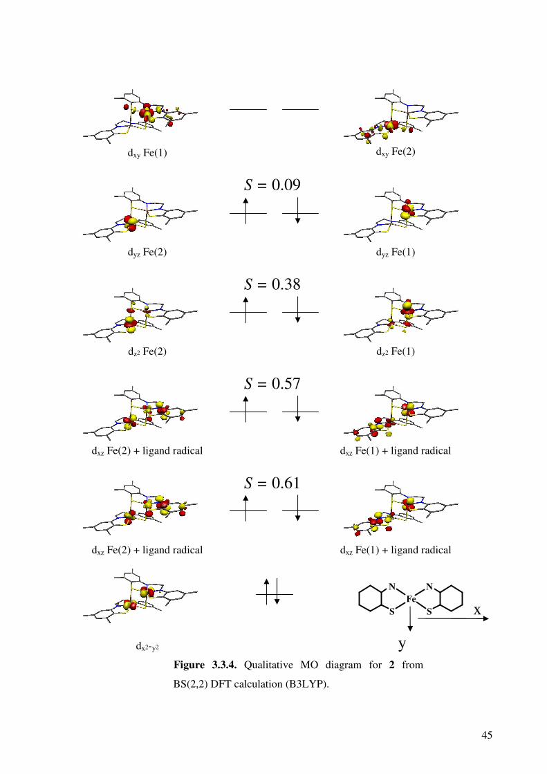
Figure 3.3.4. Qualitative MO diagram for 2 from
BS(2,2) DFT calculation (B3LYP).
dxz Fe(2) + ligand radical
dxz Fe(2) + ligand radical
dz2 Fe(2)
dyz Fe(2)
dxy Fe(1)
dxz Fe(1) + ligand radical
dxz Fe(1) + ligand radical
dyz Fe(1)
dxy Fe(2)
dz2 Fe(1)
S = 0.38
S = 0.09
S = 0.57
S = 0.61
N
S
N
S
Fe
dx2-y2
y
x

46
The qualitative molecular orbital diagram for 1 shows that each iron is a ferric species with
an intermediate spin state. It is important to note that the molecular axes are defined such that
the z axis runs from an iron centre through the axial sulfur atom and the y axis runs
equidistant between the nitrogen atoms of the ligand. This was done to give clean dxz and dyz
orbitals in the calculation output, instead of two dxz-dyz hybrid orbitals. The only effect of this
is the swapping of the dx2-y2 and dxy orbitals, so that dx2-y2 becomes lowest in energy and dxy
becomes highest in energy. In both iron atoms the lowest energy dx2-y2 is doubly occupied.
The next two higher energy molecular orbitals are a mixture of the dxz orbital of both iron
centres and the two ligand-based radicals. One of the iron dxz orbitals shares two spin-up
electrons between itself and the ligand-based radical on the opposite ligand, and these two
COs couple to two spin-down electrons based in the second iron dxz orbital and the other
ligand-based radical. Together these MOs simulate the coupling of the ligand-based π-
radicals to the iron centres. The dz2 MOs for each iron centre are singly occupied, and couple
to each other, as do the two singly occupied dyz orbitals. The orbital overlap of this coupling
is very low however, and indicates that decoupling of the electrons in the HOMO may
readily occur. Every unpaired electron is coupled, giving rise to the observed diamagnetic
ground state.
In the qualitative MO diagram of 2, the system is complicated by the fact that each
iron centre has a different axis system. The axes are defined such that for each iron the z axis
is orientated through the axial sulfur group and the y axis passes equidistant between the two
nitrogen atoms of the equatorial ligand. Thus the axes of Fe(2) are twisted 90º about the z
axis when compared to Fe(1). When treated in this manner, the electronic configuration is
exactly the same as that calculated for 1. The lowest energy dx2-y2 is doubly occupied for both
iron centres. On each iron atom the occupied dxz is mixed with a ligand orbital on the
opposite ligand, and is present in two orbitals. This indicates the presence of the ligand-based
radicals which couple to the adjacent iron dxz orbital. The HOMO-1 consists of the singly-
occupied dz2 orbital of each iron centre, which are coupled antiferromagnetically. Similarly,
the HOMO is made up of the two coupled, singly-occupied dyz orbitals of each iron. Thus it
can be seen that the compound has an overall diamagnetic ground state.
47
CHAPTER 3
Square Pyramidal Complexes of Iron
Containing Tetradentate o-Iminothionebenzosemiquinonate
Ligands and an Apical Iodide

48
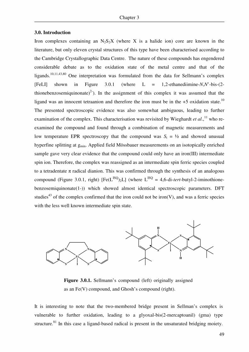
Chapter 3
49
3.0. Introduction
Iron complexes containing an N2S2X (where X is a halide ion) core are known in the
literature, but only eleven crystal structures of this type have been characterised according to
the Cambridge Crystallographic Data Centre. The nature of these compounds has engendered
considerable debate as to the oxidation state of the metal centre and that of the
ligands.10,11,43,80 One interpretation was formulated from the data for Sellmann’s complex
[FeLI] shown in Figure 3.0.1 (where L = 1,2-ethanediimine-N,N’-bis-(2-
thionebenzosemiquinonate)2-). In the assignment of this complex it was assumed that the
ligand was an innocent tetraanion and therefore the iron must be in the +5 oxidation state.10
The presented spectroscopic evidence was also somewhat ambiguous, leading to further
examination of the complex. This characterisation was revisited by Wieghardt et al.,11 who re-
examined the compound and found through a combination of magnetic measurements and
low temperature EPR spectroscopy that the compound was St = ½ and showed unusual
hyperfine splitting at gmin. Applied field Mössbauer measurements on an isotopically enriched
sample gave very clear evidence that the compound could only have an iron(III) intermediate
spin ion. Therefore, the complex was reassigned as an intermediate spin ferric species coupled
to a tetradentate π radical dianion. This was confirmed through the synthesis of an analogous
compound (Figure 3.0.1, right) [Fe(LISQ)2L] (where LISQ = 4,6-di-tert-butyl-2-iminothione-
benzosemiquinonate(1-)) which showed almost identical spectroscopic parameters. DFT
studies43 of the complex confirmed that the iron could not be iron(V), and was a ferric species
with the less well known intermediate spin state.
N
S
N
S
Fe
I
N
S N
S
Fe
H
H
I
Figure 3.0.1. Sellmann’s compound (left) originally assigned
as an Fe(V) compound, and Ghosh’s compound (right).
It is interesting to note that the two-membered bridge present in Sellman’s complex is
vulnerable to further oxidation, leading to a glyoxal-bis(2-mercaptoanil) (gma) type
structure.81 In this case a ligand-based radical is present in the unsaturated bridging moiety.

Chapter 3
50
An advantage of using a ligand with a propyl group bridge is that this oxidative
rearrangement is avoided, and the two π radicals are isolated from one another.
The work presented here utilises 1,3-propanediamine-N,N’-bis(2-benzenethiol) (1LH4)
and 1,2-bis(2-mercapto-3,5-di-tert-butylaniline)ethane (2LH4) in order to synthesise two
compounds with similar structural motifs. The synthesised compounds were then examined
with a variety of spectroscopic and physical methods in order to determine the oxidation state
at the metal centre and that of the ligands, and to observe the effect of using a propyl bridge
instead of the shorter, less stable ethyl bridge. The synthesis of the compound with 2LH4
essentially gave an analogue of Sellmann’s complex, but with a greater solubility which
would prove useful in applied field Mössbauer spectroscopy. Thus both complexes were
found by spectroscopic, physical and DFT methods to consist of an iron(III) ion coordinated
to a ligand containing two o-iminothionebenzosemiquinonate π radicals.
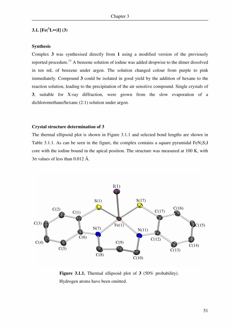
Chapter 3
51
3.1. [Fe(1L••)I] (3)
Synthesis
Complex 3 was synthesised directly from 1 using a modified version of the previously
reported procedure.11 A benzene solution of iodine was added dropwise to the dimer dissolved
in ten mL of benzene under argon. The solution changed colour from purple to pink
immediately. Compound 3 could be isolated in good yield by the addition of hexane to the
reaction solution, leading to the precipitation of the air sensitive compound. Single crystals of
3, suitable for X-ray diffraction, were grown from the slow evaporation of a
dichloromethane/hexane (2:1) solution under argon.
Crystal structure determination of 3
The thermal ellipsoid plot is shown in Figure 3.1.1 and selected bond lengths are shown in
Table 3.1.1. As can be seen in the figure, the complex contains a square pyramidal FeN2S2I
core with the iodine bound in the apical position. The structure was measured at 100 K, with
3σ values of less than 0.012 Å.
Figure 3.1.1. Thermal ellipsoid plot of 3 (50% probability).
Hydrogen atoms have been omitted.
S(1)
C(1) C(2)
C(3)
C(4)
C(5)
C(6)
N(7)
C(8)
C(9)
C(10)
N(11)
C(12)
C(13) C(14)
C(15)
C(16) C(17)
S(17)
I(1)
Fe(1)
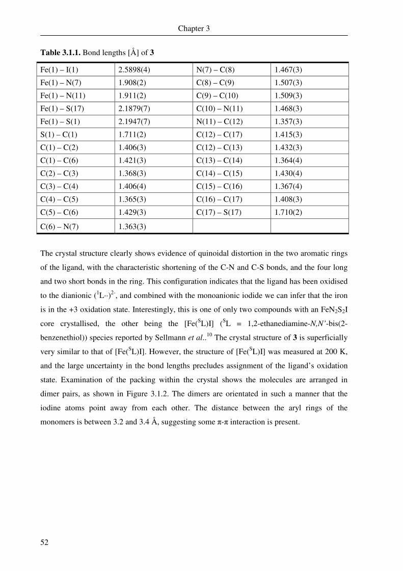
Chapter 3
52
Table 3.1.1. Bond lengths [Å] of 3
Fe(1) – I(1) 2.5898(4) N(7) – C(8) 1.467(3)
Fe(1) – N(7) 1.908(2) C(8) – C(9) 1.507(3)
Fe(1) – N(11) 1.911(2) C(9) – C(10) 1.509(3)
Fe(1) – S(17) 2.1879(7) C(10) – N(11) 1.468(3)
Fe(1) – S(1) 2.1947(7) N(11) – C(12) 1.357(3)
S(1) – C(1) 1.711(2) C(12) – C(17) 1.415(3)
C(1) – C(2) 1.406(3) C(12) – C(13) 1.432(3)
C(1) – C(6) 1.421(3) C(13) – C(14) 1.364(4)
C(2) – C(3) 1.368(3) C(14) – C(15) 1.430(4)
C(3) – C(4) 1.406(4) C(15) – C(16) 1.367(4)
C(4) – C(5) 1.365(3) C(16) – C(17) 1.408(3)
C(5) – C(6) 1.429(3) C(17) – S(17) 1.710(2)
C(6) – N(7) 1.363(3)
The crystal structure clearly shows evidence of quinoidal distortion in the two aromatic rings
of the ligand, with the characteristic shortening of the C-N and C-S bonds, and the four long
and two short bonds in the ring. This configuration indicates that the ligand has been oxidised
to the dianionic (1L··)2-, and combined with the monoanionic iodide we can infer that the iron
is in the +3 oxidation state. Interestingly, this is one of only two compounds with an FeN2S2I
core crystallised, the other being the [Fe(SL)I] (SL = 1,2-ethanediamine-N,N’-bis(2-
benzenethiol)) species reported by Sellmann et al..10 The crystal structure of 3 is superficially
very similar to that of [Fe(SL)I]. However, the structure of [Fe(SL)I] was measured at 200 K,
and the large uncertainty in the bond lengths precludes assignment of the ligand’s oxidation
state. Examination of the packing within the crystal shows the molecules are arranged in
dimer pairs, as shown in Figure 3.1.2. The dimers are orientated in such a manner that the
iodine atoms point away from each other. The distance between the aryl rings of the
monomers is between 3.2 and 3.4 Å, suggesting some π-π interaction is present.

Chapter 3
53
Figure 3.1.2. Crystal packing of 3. Ellipsoids are shown at
50% level and hydrogen atoms are excluded.
Electronic absorption spectroscopy
The electronic spectrum of 3 measured in dichloromethane at room temperature is shown in
Figure 3.1.2. The intense purple solution is dominated by a large absorption at 561 nm, with
an extinction coefficient of 11,800 M-1 cm-1. This peak is far too intense to be assigned as a
d-d transition, and closely resembles previously assigned spin- and dipole-allowed charge-
transfer (CT) transitions.11,36,82,83 The appearance of this band is characteristic for the N,S-
coordination of two o-iminothionebenzosemiquinonato(1-) ligands. Thus, in this present case
the CT band indicates that both halves of the ligand are oxidised by one electron to give two π
radicals.
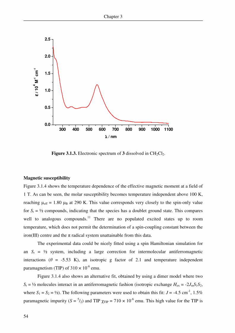
Chapter 3
54
300 400 500 600 700 800 900 1000 11000.0
0.5
1.0
1.5
2.0
2.5εε εε
/ /
/
/ 1
04 M
-1 c
m-1
λλλλ / nm
Figure 3.1.3. Electronic spectrum of 3 dissolved in CH2Cl2.
Magnetic susceptibility
Figure 3.1.4 shows the temperature dependence of the effective magnetic moment at a field of
1 T. As can be seen, the molar susceptibility becomes temperature independent above 100 K,
reaching µeff = 1.80 µB at 290 K. This value corresponds very closely to the spin-only value
for St = ½ compounds, indicating that the species has a doublet ground state. This compares
well to analogous compounds.11 There are no populated excited states up to room
temperature, which does not permit the determination of a spin-coupling constant between the
iron(III) centre and the π radical system unattainable from this data.
The experimental data could be nicely fitted using a spin Hamiltonian simulation for
an St = ½ system, including a large correction for intermolecular antiferromagnetic
interactions (θ = -5.53 K), an isotropic g factor of 2.1 and temperature independent
paramagnetism (TIP) of 310 × 10-6 emu.
Figure 3.1.4 also shows an alternative fit, obtained by using a dimer model where two
St = ½ molecules interact in an antiferromagnetic fashion (isotropic exchange Hex = -2JmS1S2,
where S1 = S2 = ½). The following parameters were used to obtain this fit: J = -4.5 cm-1, 1.5%
paramagnetic impurity (S = 5/2) and TIP χTIP = 710 × 10-6 emu. This high value for the TIP is

Chapter 3
55
probably an effective value which accounts for an impurity consisting of single-domain
ferromagnetic particles and is not an authentic TIP value. This model is given credence
through observation of the dimer pairs in the X-ray crystal structure and is a more accurate
picture.
0 50 100 150 200 250 300
1.0
1.2
1.4
1.6
1.8
µµ µµe
ff / µµ µµ
B
T / K
0 50 100 150 200 250 300
1.0
1.2
1.4
1.6
1.8
2.0
2.2
2.4
2.6
2.8
µµ µµe
ff / µµ µµ
BT / K
Figure 3.1.4. Temperature dependence of the effective
magnetic moment of a solid sample of 3 measured at 1 T. Two
simulations are shown; the first simulation is of a monomeric
St = ½ species (left). The second simulation uses a dimer
model, where two independent St = ½ molecules interact
antiferromagnetically (right). Full simulation parameters are
given in the text.
EPR spectroscopy
The X-band EPR spectrum of a frozen solution of 3 in CH2Cl2/toluene was recorded at 30 K
and is shown in Figure 3.1.5. The recorded spectrum shows a well-resolved rhombic signal
around g = 2. The large anisotropy of the signal (gmax = 2.285, gmid = 2.119, gmin = 2.037)
arises from spin-orbit interactions, indicating significant spin density at the iron centre. All
three g values are larger than two, which signifies the iron(III) centre can not have a low spin
electronic configuration.65 Therefore, in order to have a St = ½, the compound must have an
intermediate spin iron centre which couples antiferromagnetically to two ligand-based π
radicals.

Chapter 3
56
Figure 3.1.5. The X-band EPR spectrum of 3 in a frozen
CH2Cl2/toluene solution (10:1 v/v) measured at 30 K.
Conditions: frequency 9.450 GHz, power 1.001 mW,
modulation 10 G.
The spectrum also shows an interesting hyperfine splitting pattern at gmin, which has
previously been observed in other compounds of this type.11 This splitting could be simulated
by taking into account a hyperfine interaction with the apical 127I nucleus (I = 5/2; 100%
natural abundance). As the 127I nucleus has I > ½, there is a non-spherical electric charge in
the nucleus. Nuclear electric quadrupole interactions are induced by the nuclear quadrupole
moment Q interacting with a non-zero electric field gradient (EFG). The EFG of the
asymmetric charge distribution interacts with the nuclear electric (quadrupole) and nuclear
electric moment of the iodine nucleus.
Usually, quadrupole effects are not observed in the EPR if the nuclear hyperfine
coupling tensor (A) and the EFG coupling tensor (P) are co-aligned. This collinearity results
in a second-order shift of energy levels, in which all energy levels are displaced by a constant
value. This produces no change in the observed spectrum, and the coupling of the iodine
nucleus to the electron would lead to six equivalent transitions. This is, however, clearly not
the case. The large nuclear electric quadrupole interactions cause the shifting and mixing of
the nuclear spin states mI. This in turn affects transition probabilities and forbidden
transitions become visible, where ∆mI > 0. Note also the intensities of the lines and the
spacings between them are not equivalent. This is readily apparent in the magnification of
gmin shown in Figure 3.1.6.
260 280 300 320 340 360
2.6 2.5 2.4 2.3 2.2 2.1 2 1.9 1.8
dχχ χχ''/
dB
B [mT]
Sim
Exp
g - values

Chapter 3
57
325 330 335 340 345
2.1 2.08 2.06 2.04 2.02 2 1.98 1.96
dχ''/
dB
B [mT]
Sim
Exp
g - values
Figure 3.1.6. Magnification of gmin from the EPR spectrum of
3.
Parameters for the simulation are found in Table 3.1.2. The major components of the
EFG coupling tensor are found in the direction of gmax and gmid, orientated away from Amax
(along gmin).
Table 3.1.2. Spin Hamiltonian Parameters of 3 from the EPR simulation shown in Figure
3.1.5a
g 2.285, 2.119, 2.037
Ab [10-4 cm-1] 3, 4, -60
Pc [10-4 cm-1] 25.0, -35.0, 2.0
Wd [10-4 cm-1] 90, 70, 24
Ligand nucleus 127I
Nuclear spin I 5/2
Nuclear factor gN 1.13
Qe, |e| × [10-24 cm2] -0.789
a) The order of the A and V components is given with respect to the g tensors gmax, gmid and gmin. b) The A-tensor
components, the signs are arbitrary, they cannot be determined from the simulation. c) The EFG tensor
components, the signs are again arbitrary. d) Line width, Gaussian distribution. e) Quadrupole moment of the
iodine nucleus.
Chapter 3
58
This has been observed previously,11 and one possible explanation for non-collinearity of the
A and P tensors developed. The covalent interactions between the pz, py and px orbitals of the
iodine and the respective dz2, dyz and dxz orbitals of the iron are the origin of the major EFG
component at the iodine. The dz2 of the iron and the pz orbital of the iodine have a strong σ-
interaction, while the dxz - px, and the dyz - py orbitals have much weaker π interactions.
Therefore the main component of the EFG tensor at the iodide nucleus lies in the z direction.
Interestingly the dz2, dyz and dxz orbitals of the iron, which are engaged in bonding to the
apical iodide, are all singly occupied; the p-shell spin density at the iodine should be similar
to the charge anisotropy at the iodine and the EFG and hyperfine coupling tensors collinear.
In 3 we have postulated the presence of two ligand-based π radicals, and these
antiferromagnetically coupled radicals transfer spin density into the dxz and dyz orbitals. This
causes magnetic anisotropy between the dz2, dyz and dxz orbitals, which in turn induces
anisotropy in the spin density of the p orbitals of the iodine. It should be noted that this
explanation does not account for the large asymmetry in the x and y components of the P
tensor, the origin of which is unknown.
The quadrupole interaction of the iodine with the unpaired electron based on the iron
also indicates a considerable level of covalency between the iron and the apical ligand. This
misalignment of the EFG and hyperfine coupling tensors has previously been recognized as a
possible marker for the presence of semiquinonate radical monoanions in iron complexes
containing either an iodine or bromine ligand.11,84
As can been seen, the EPR spectrum of 3 provides a considerable amount of
information about the bonding at the iron. The spectrum confirms the doublet ground state,
and also provides affirmation for the existence of two ligand-based π radicals which couple
antiferromagnetically to an intermediate spin ferric centre.

Chapter 3
59
Mössbauer spectroscopy
The zero-field Mössbauer spectrum recorded at 80 K and a measurement with an applied
field of 7 T at 4.2 K of solid 3 are shown in Figure 3.1.7.
Figure 3.1.7. Mössbauer spectra of 3, zero-field measurement
at 80 K (left) and with an applied field of 7 T at 4.2 K (right).
The zero-field Mössbauer spectrum of 3 shows an intense doublet with an isomer shift of
0.22 mm s-1 and a quadrupole splitting (∆EQ) of 3.10 mm s-1. This is within the typical range
established for intermediate spin iron(III) species. A second doublet can be seen with an
isomer shift of 0.46 mm s-1, which corresponds to 9% of a high spin iron(III) impurity. The
applied field measurement of the solid, however, gives a diamagnetic spectrum, and can be
simulated using the previously discussed parameters and a St = 0 ground state. This is due to
rather strong intermolecular coupling in the solid state leading to the complete cancellation of
the internal field at the iron centre. This is not wholly surprising, as intermolecular
antiferromagnetic coupling was observed at low temperature in the magnetic susceptibility
measurements. Unfortunately the limited solubility of the compound precluded dissolution to
the extent required for frozen solution Mössbauer spectroscopic measurements.
Summary
The spectroscopic and physical evidence collected for compound 3 confirms that the
complex consists of a five-coordinate square pyramidal intermediate spin ferric species with
an iodide bound to the axial position and the N2S2-ligand (1L) occupying the equatorial plane.
The X-ray crystallography results indicate that 1L is doubly oxidised to give (1L••)2- and
-4 -2 0 2 4
0.86
0.88
0.90
0.92
0.94
0.96
0.98
1.00
δ = 0.22 mm s-1
∆EQ= |3.10| mm s
-1
Re
lati
ve
Tra
nsm
iss
ion
Velocity [mm s-1]
-5 0 5
0.944
0.952
0.960
0.968
0.976
0.984
0.992
1.000
Velocity [mm s-1]
7.0 T, 4 K
Re
lati
ve
Tra
nsm
iss
ion
Chapter 3
60
contains two ligand-based π radicals. The crystal structure also shows the compounds are
arranged into dimeric structures, providing a pathway for an intermolecular,
antiferromagnetic interaction.
SQUID measurements indicate that the compound has a doublet ground state and no
excited states are populated up to room temperature. At low temperature evidence of
intermolecular interactions is observed, which can be simulated either using an St = 1/2
species with a Theta Weiss constant as a correction for the intermolecular interaction, or
using a dimer model of two St = 1/2 species that are antiferromagnetically coupled with a
small coupling constant of J = -4.5 cm-1.
The EPR spectrum confirms the St = ½ ground state, and indicates that the unpaired
electron is based at the iron centre, due to a large anisotropy in g values. The three values for
the g tensor are all greater two, which establishes that the iron centre can not be low spin
iron(III), ruling out one possible electronic structure. An interesting hyperfine feature at gmin
could also be successfully simulated by taking into account the quadrupole interaction of the
apical iodine with unpaired electron at the iron centre. This is a marker for an intermediate
spin ferric species coupled to two π radicals with an apical iodide or bromide. It also
indicates significant covalency between the iodide and the iron core.
Conversely, the Mössbauer spectra are more ambiguous. While the isomer shift and
quadrupole splitting values are characteristic for an intermediate spin iron(III), several other
oxidation and spin states also give rise to similar parameters. The applied field measurement
showed a diamagnetic spectrum, as a result of intermolecular interactions within the dimers
causing the complete cancellation of the internal field at the iron nucleus.
However, the compound very closely resembles the previously characterised Ghosh
compound11 and the Sellmann compound10 shown in Figure 3.0.1. These compounds show
very similar spectroscopic measurements, even though the architecture of the ligand changes
across the series. The Ghosh compound has no unit bridging the two
o-iminothionesemiquinonate(1-) groups, the Sellmann complex has a saturated 2-carbon
bridge and 3 contains a saturated 3-carbon bridge. Thus, it can be concluded that the bridging
group plays no role in affecting the electronic configuration of this class of compounds.
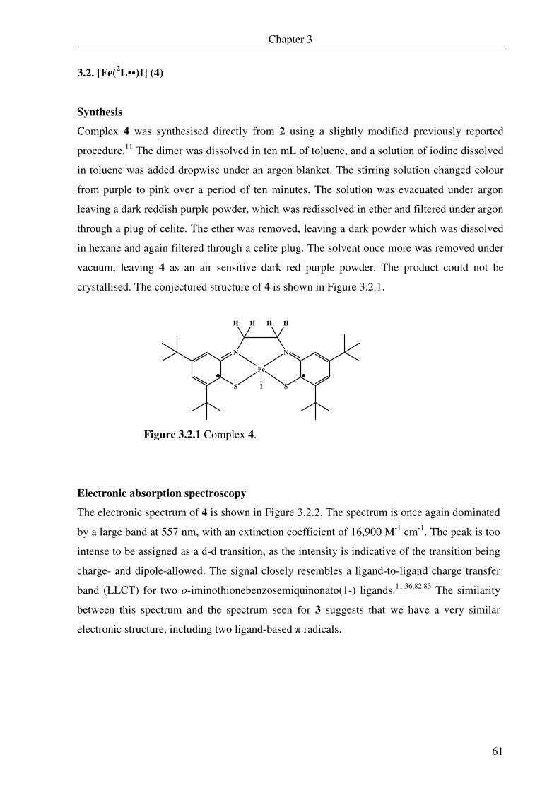
Chapter 3
61
3.2. [Fe(2L••)I] (4)
Synthesis
Complex 4 was synthesised directly from 2 using a slightly modified previously reported
procedure.11 The dimer was dissolved in ten mL of toluene, and a solution of iodine dissolved
in toluene was added dropwise under an argon blanket. The stirring solution changed colour
from purple to pink over a period of ten minutes. The solution was evacuated under argon
leaving a dark reddish purple powder, which was redissolved in ether and filtered under argon
through a plug of celite. The ether was removed, leaving a dark powder which was dissolved
in hexane and again filtered through a celite plug. The solvent once more was removed under
vacuum, leaving 4 as an air sensitive dark red purple powder. The product could not be
crystallised. The conjectured structure of 4 is shown in Figure 3.2.1.
N
S
N
S
Fe
I
H H HH
Figure 3.2.1 Complex 4.
Electronic absorption spectroscopy
The electronic spectrum of 4 is shown in Figure 3.2.2. The spectrum is once again dominated
by a large band at 557 nm, with an extinction coefficient of 16,900 M-1 cm-1. The peak is too
intense to be assigned as a d-d transition, as the intensity is indicative of the transition being
charge- and dipole-allowed. The signal closely resembles a ligand-to-ligand charge transfer
band (LLCT) for two o-iminothionebenzosemiquinonato(1-) ligands.11,36,82,83 The similarity
between this spectrum and the spectrum seen for 3 suggests that we have a very similar
electronic structure, including two ligand-based π radicals.

Chapter 3
62
Figure 3.2.2. Electronic spectrum of 4 dissolved in CH2Cl2.
Magnetic susceptibility
The temperature dependence of the magnetic moment is shown in Figure 3.2.3.
0 50 100 150 200 250 300
1.0
1.2
1.4
1.6
1.8
µµ µµe
ff / µµ µµ
B
T / K
0 50 100 150 200 250 300
1.0
1.2
1.4
1.6
1.8
2.0
2.2
2.4
2.6
2.8
µµ µµeff /
µµ µµB
T / K
Figure 3.2.3. Temperature dependence of the magnetic
moment of a solid sample of 4 measured at 1 T. Two
simulations are shown; the first simulation is of a monomeric St
= ½ species with Weiss’ constant θ to simulate some inter-
molecular exchange interactions (left). The second simulation
uses a dimer model, where two independent St = ½ molecules
interact antiferromagnetically (right). Full simulation
parameters are given in the text.
300 400 500 600 700 800 900 1000 11000.0
0.5
1.0
1.5
2.0
2.5
3.0
3.5εε εε
/ /
/
/ 1
04 M
-1 c
m-1
λλλλ / nm
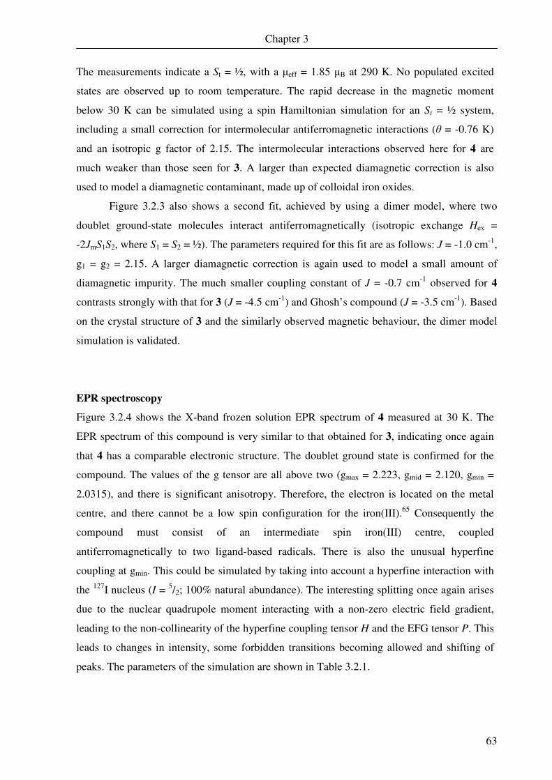
Chapter 3
63
The measurements indicate a St = ½, with a µeff = 1.85 µB at 290 K. No populated excited
states are observed up to room temperature. The rapid decrease in the magnetic moment
below 30 K can be simulated using a spin Hamiltonian simulation for an St = ½ system,
including a small correction for intermolecular antiferromagnetic interactions (θ = -0.76 K)
and an isotropic g factor of 2.15. The intermolecular interactions observed here for 4 are
much weaker than those seen for 3. A larger than expected diamagnetic correction is also
used to model a diamagnetic contaminant, made up of colloidal iron oxides.
Figure 3.2.3 also shows a second fit, achieved by using a dimer model, where two
doublet ground-state molecules interact antiferromagnetically (isotropic exchange Hex =
-2JmS1S2, where S1 = S2 = ½). The parameters required for this fit are as follows: J = -1.0 cm-1,
g1 = g2 = 2.15. A larger diamagnetic correction is again used to model a small amount of
diamagnetic impurity. The much smaller coupling constant of J = -0.7 cm-1 observed for 4
contrasts strongly with that for 3 (J = -4.5 cm-1) and Ghosh’s compound (J = -3.5 cm-1). Based
on the crystal structure of 3 and the similarly observed magnetic behaviour, the dimer model
simulation is validated.
EPR spectroscopy
Figure 3.2.4 shows the X-band frozen solution EPR spectrum of 4 measured at 30 K. The
EPR spectrum of this compound is very similar to that obtained for 3, indicating once again
that 4 has a comparable electronic structure. The doublet ground state is confirmed for the
compound. The values of the g tensor are all above two (gmax = 2.223, gmid = 2.120, gmin =
2.0315), and there is significant anisotropy. Therefore, the electron is located on the metal
centre, and there cannot be a low spin configuration for the iron(III).65 Consequently the
compound must consist of an intermediate spin iron(III) centre, coupled
antiferromagnetically to two ligand-based radicals. There is also the unusual hyperfine
coupling at gmin. This could be simulated by taking into account a hyperfine interaction with
the 127I nucleus (I = 5/2; 100% natural abundance). The interesting splitting once again arises
due to the nuclear quadrupole moment interacting with a non-zero electric field gradient,
leading to the non-collinearity of the hyperfine coupling tensor H and the EFG tensor P. This
leads to changes in intensity, some forbidden transitions becoming allowed and shifting of
peaks. The parameters of the simulation are shown in Table 3.2.1.
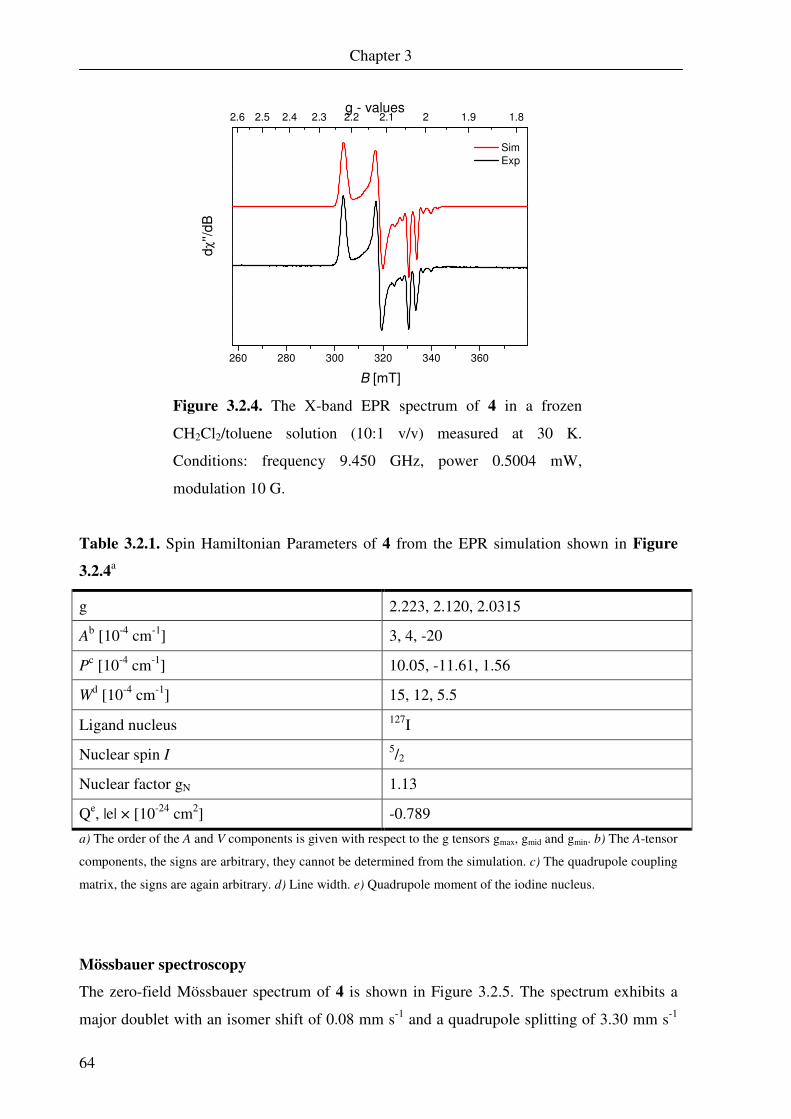
Chapter 3
64
Figure 3.2.4. The X-band EPR spectrum of 4 in a frozen
CH2Cl2/toluene solution (10:1 v/v) measured at 30 K.
Conditions: frequency 9.450 GHz, power 0.5004 mW,
modulation 10 G.
Table 3.2.1. Spin Hamiltonian Parameters of 4 from the EPR simulation shown in Figure
3.2.4a
g 2.223, 2.120, 2.0315
Ab [10-4 cm-1] 3, 4, -20
Pc [10-4 cm-1] 10.05, -11.61, 1.56
Wd [10-4 cm-1] 15, 12, 5.5
Ligand nucleus 127I
Nuclear spin I 5/2
Nuclear factor gN 1.13
Qe, |e| × [10-24 cm2] -0.789
a) The order of the A and V components is given with respect to the g tensors gmax, gmid and gmin. b) The A-tensor
components, the signs are arbitrary, they cannot be determined from the simulation. c) The quadrupole coupling
matrix, the signs are again arbitrary. d) Line width. e) Quadrupole moment of the iodine nucleus.
Mössbauer spectroscopy
The zero-field Mössbauer spectrum of 4 is shown in Figure 3.2.5. The spectrum exhibits a
major doublet with an isomer shift of 0.08 mm s-1 and a quadrupole splitting of 3.30 mm s-1
260 280 300 320 340 360
2.6 2.5 2.4 2.3 2.2 2.1 2 1.9 1.8g - values
dχ''/
dB
B [mT]
Sim
Exp
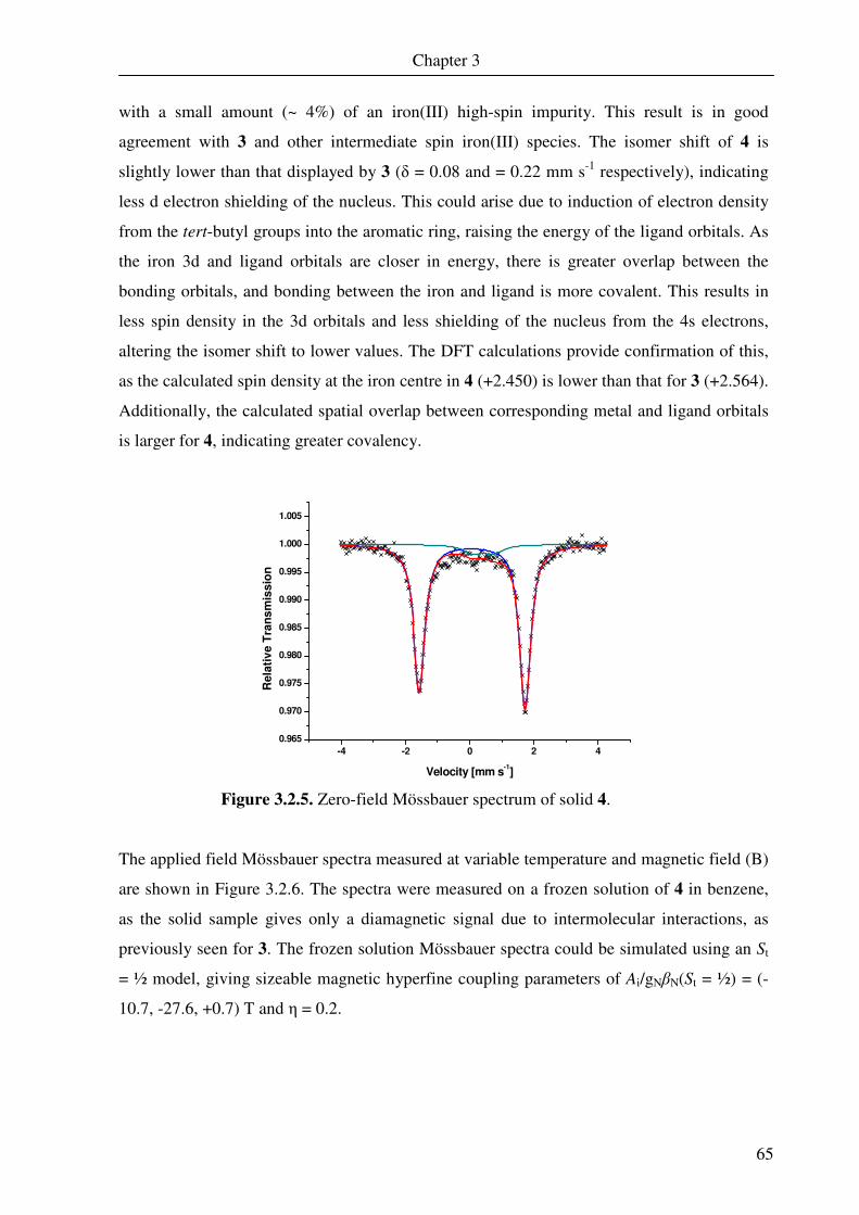
Chapter 3
65
with a small amount (~ 4%) of an iron(III) high-spin impurity. This result is in good
agreement with 3 and other intermediate spin iron(III) species. The isomer shift of 4 is
slightly lower than that displayed by 3 (δ = 0.08 and = 0.22 mm s-1 respectively), indicating
less d electron shielding of the nucleus. This could arise due to induction of electron density
from the tert-butyl groups into the aromatic ring, raising the energy of the ligand orbitals. As
the iron 3d and ligand orbitals are closer in energy, there is greater overlap between the
bonding orbitals, and bonding between the iron and ligand is more covalent. This results in
less spin density in the 3d orbitals and less shielding of the nucleus from the 4s electrons,
altering the isomer shift to lower values. The DFT calculations provide confirmation of this,
as the calculated spin density at the iron centre in 4 (+2.450) is lower than that for 3 (+2.564).
Additionally, the calculated spatial overlap between corresponding metal and ligand orbitals
is larger for 4, indicating greater covalency.
Figure 3.2.5. Zero-field Mössbauer spectrum of solid 4.
The applied field Mössbauer spectra measured at variable temperature and magnetic field (B)
are shown in Figure 3.2.6. The spectra were measured on a frozen solution of 4 in benzene,
as the solid sample gives only a diamagnetic signal due to intermolecular interactions, as
previously seen for 3. The frozen solution Mössbauer spectra could be simulated using an St
= ½ model, giving sizeable magnetic hyperfine coupling parameters of Ai/gNβN(St = ½) = (-
10.7, -27.6, +0.7) T and η = 0.2.
-4 -2 0 2 4
0.965
0.970
0.975
0.980
0.985
0.990
0.995
1.000
1.005
Rela
tiv
e T
ran
sm
iss
ion
Velocity [mm s-1]
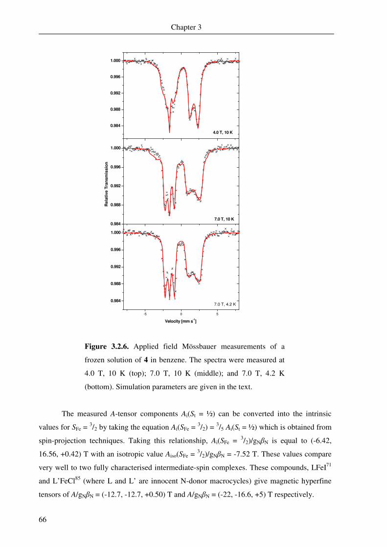
Chapter 3
66
Figure 3.2.6. Applied field Mössbauer measurements of a
frozen solution of 4 in benzene. The spectra were measured at
4.0 T, 10 K (top); 7.0 T, 10 K (middle); and 7.0 T, 4.2 K
(bottom). Simulation parameters are given in the text.
The measured A-tensor components Ai(St = ½) can be converted into the intrinsic
values for SFe = 3/2 by taking the equation Ai(SFe = 3/2) = 3/5 Ai(St = ½) which is obtained from
spin-projection techniques. Taking this relationship, Ai(SFe = 3/2)/gNβN is equal to (-6.42,
16.56, +0.42) T with an isotropic value Aiso(SFe = 3/2)/gNβN = -7.52 T. These values compare
very well to two fully characterised intermediate-spin complexes. These compounds, LFeI71
and L’FeCl85 (where L and L’ are innocent N-donor macrocycles) give magnetic hyperfine
tensors of A/gNβN = (-12.7, -12.7, +0.50) T and A/gNβN = (-22, -16.6, +5) T respectively.
0.984
0.988
0.992
0.996
1.000
7.0 T, 10 K
Re
lati
ve
Tra
ns
mis
sio
n
-5 0 5
0.984
0.988
0.992
0.996
1.000
7.0 T, 4.2 K
Velocity [mm s-1]
0.984
0.988
0.992
0.996
1.000
4.0 T, 10 K
Chapter 3
67
Interestingly, this magnetic hyperfine coupling configuration with an atypically small
positive z component of the A tensor at the 57Fe nucleus have previously been reported for
other well-characterised iron(III) intermediate-spin compounds.11,86-88 The positive A tensor
minor component and a quadrupole splitting greater than +3 mm s-1 have long been
documented as distinguishing features of iron(III) in an intermediate-spin spin state.89,90
Summary
The spectroscopic and magnetic data collected on compound 4 indicate that the complex
does in fact consist of an iron(III) ion bound to (2L••)2- in the equatorial plane and an apical
iodine. Unfortunately there is no X-ray structure to corroborate the structural claims and to
assign an oxidation state to the ligand. However, a combination of mass spectroscopy and
elemental analysis allow this preliminary assignment of the structure.
The electronic structure is almost identical to that of 3, signifying the electronic states
of 3 and 4 are very similar. Both are dominated by a large band at λ ≈ 560 nm, with
extinction coefficients in excess of 10,000 M-1 cm-1. These are very similar to bands
previously assigned to ligand to ligand charge transitions in compounds containing two
ligand-based π radicals.
The magnetic susceptibility measurements at variable temperature show that the
compound has a doublet ground state. The SQUID can be simulated by using either an St = ½
system with a small Theta Weiss correction to model intermolecular interactions, or a dimer
structure of two antiferromagnetically coupled St = 1/2 species with a small coupling constant
of -1.0 cm-1.
The EPR spectrum of the compound confirms the St = ½ ground state. The large
anisotropy of the signal indicates that the unpaired electron is found on the iron centre. As
the three g values are all above two, the possibility of the iron having a low-spin spin state
can be eliminated. A further indication of intermediate-spin state of the iron(III) coupled to
two ligand π radicals can be found in the unusual hyperfine coupling pattern at gmin. This
arises out of the EFG tensor of the iodine being aligned “off” from the hyperfine coupling
tensor, causing mixing of states and the appearance of new transitions. As noted earlier, this
is strongly indicative of the presence of two ligand radicals and an intermediate state iron.
The zero-field Mössbauer spectrum measured gives a classic intermediate spin
iron(III) signal, though this alone is not enough to assign the spin state at the iron
unambiguously. The applied field measurements made at variable temperatures confirm
Chapter 3
68
through the magnetic hyperfine coupling parameters of the 57Fe nucleus that the iron centre
does have an intermediate spin state. Due to the similarities in the spectroscopy between 3
and 4, we can surmise that compound 3 has similar hyperfine coupling factors.
3.3. DFT calculations of 3 and 4
In order to further examine complexes 3 and 4, detailed theoretical calculations involving
density functional theory (DFT) have been performed using the Orca package.76 Scalar
relativistic corrections for iodine have been taken into account using the ZORA method91,
and full details of the calculation methods are given in chapter 7. A useful method allowed
by Orca is calculation of broken-symmetry (BS) solutions, whereby unpaired electron density
can be found on various parts of the complex in question. This is particularly practical for
calculating the lowest energy geometric and electronic state for compounds where a ligand
radical is suspected. A useful indicator for this situation found within the calculation is the
spin-expectation value ⟨S2⟩. A value for ⟨S2⟩ that differs considerably from the value S(S+1)
for a pure spin state (where S is the total spin) indicates that an irregular spin state, such as a
BS solution, has been found.43 Unrestricted Kohn-Sham solutions for both 3 and 4 were
calculated and the obtained ⟨S2⟩ values were found to be 2.11 and 2.00 respectively, differing
considerably from the expected value of 0.75 for an S = ½ compound.
The BS-DFT methodology was applied to 3 and 4, with comparison of the calculated
Mössbauer parameters78 to experimental values, and in the case of 4 comparison of geometry
optimised bond lengths. It has been revealed that 3 and 4 consist of a square pyramidal
intermediate spin iron(III) centre which is coupled antiferromagnetically to two ligand-based
radicals. Broken symmetry calculations have been carried out previously on this type of
complex,25,43 using the B3LYP functional under a BS(3,2) DFT calculation. The (3,2) refers
to the unpaired electrons at a various centres, and in this case it denotes three unpaired
electrons on the iron and two unpaired electrons on the ligand. In the case of 3 and 4 a similar
method was used.
Shown in Table 3.3.1 is a comparison of the bond lengths between the BS(3,2) DFT
calculation and the experimental bond lengths of 3. Figure 3.3.1 shows the numbering of the
atoms in the molecule for reference. As can be seen, the bond lengths are in excellent
agreement between the calculation and the crystal structure, with an average difference
around the rings and bridging moiety of 0.009 Å and excellent reproduction of the semi-
quinoidal bond length pattern around the aromatic rings. The calculated bond lengths
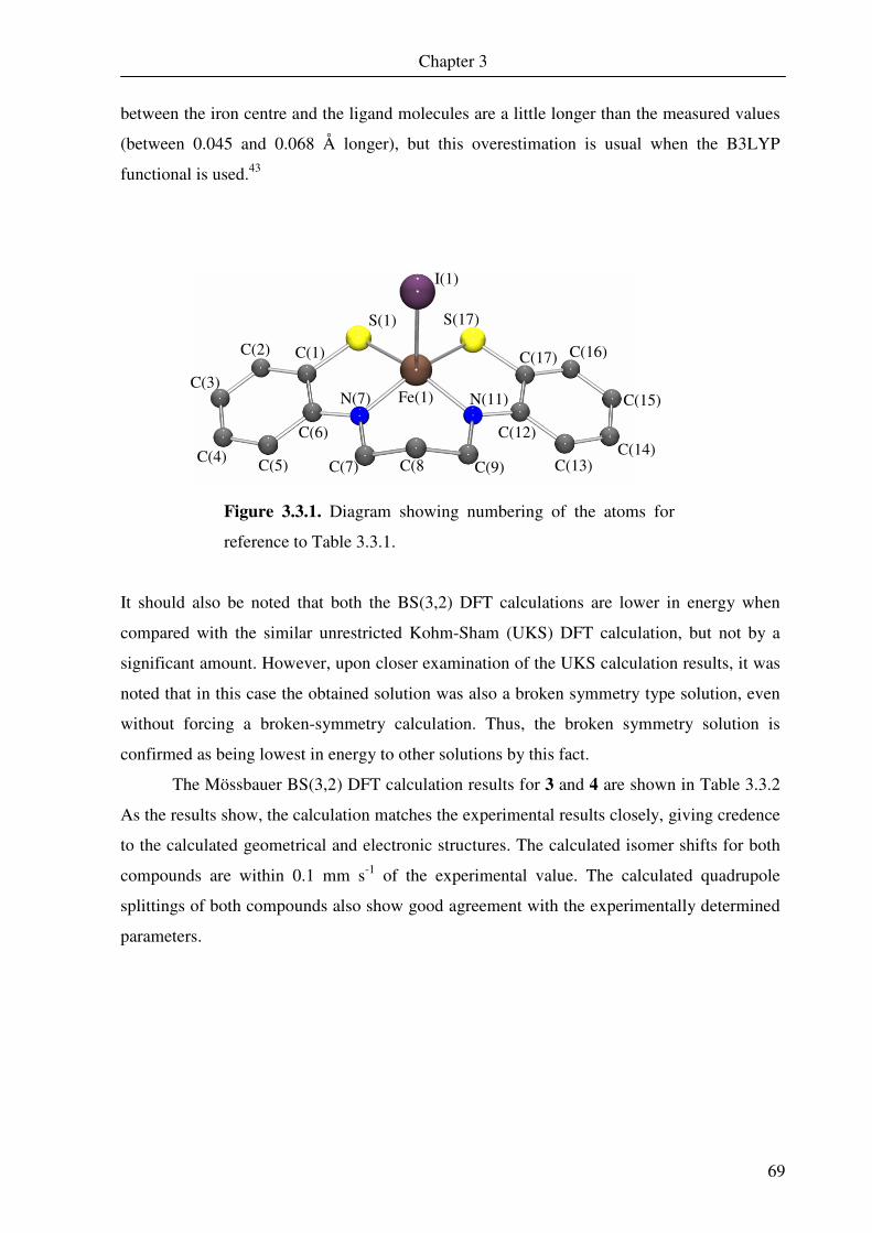
Chapter 3
69
between the iron centre and the ligand molecules are a little longer than the measured values
(between 0.045 and 0.068 Å longer), but this overestimation is usual when the B3LYP
functional is used.43
Figure 3.3.1. Diagram showing numbering of the atoms for
reference to Table 3.3.1.
It should also be noted that both the BS(3,2) DFT calculations are lower in energy when
compared with the similar unrestricted Kohm-Sham (UKS) DFT calculation, but not by a
significant amount. However, upon closer examination of the UKS calculation results, it was
noted that in this case the obtained solution was also a broken symmetry type solution, even
without forcing a broken-symmetry calculation. Thus, the broken symmetry solution is
confirmed as being lowest in energy to other solutions by this fact.
The Mössbauer BS(3,2) DFT calculation results for 3 and 4 are shown in Table 3.3.2
As the results show, the calculation matches the experimental results closely, giving credence
to the calculated geometrical and electronic structures. The calculated isomer shifts for both
compounds are within 0.1 mm s-1 of the experimental value. The calculated quadrupole
splittings of both compounds also show good agreement with the experimentally determined
parameters.
S(1)
C(1) C(2)
C(3)
C(5)
C(6)
N(7)
C(8 C(9)
N(11)
C(12)
C(13)
C(16)
Fe(1)
C(17)
S(17)
C(4) C(7)
I(1)
C(15)
C(14)

Chapter 3
70
Table 3.3.1. Comparison of bond lengths [Å] between the geometry optimisation of the
BS(3,2) DFT calculation and the experimental values obtained from single crystal X-ray
measurements.
Experimental values BS(3,2) calculation
Fe(1) – I(1) 2.5898(4) 2.649
Fe(1) – N(7) 1.908(2) 1.956
Fe(1) – N(11) 1.911(2) 1.956
Fe(1) – S(17) 2.1879(7) 2.256
Fe(1) – S(1) 2.1947(7) 2.256
S(1) – C(1) 1.711(2) 1.720
C(1) – C(2) 1.406(3) 1.416
C(1) – C(6) 1.421(3) 1.436
C(2) – C(3) 1.368(3) 1.378
C(3) – C(4) 1.406(4) 1.416
C(4) – C(5) 1.365(3) 1.375
C(5) – C(6) 1.429(3) 1.431
C(6) – N(7) 1.363(3) 1.354
N(7) – C(8) 1.467(3) 1.465
C(8) – C(9) 1.507(3) 1.519
C(9) – C(10) 1.509(3) 1.520
C(10) – N(11) 1.468(3) 1.465
N(11) – C(12) 1.357(3) 1.354
C(12) – C(17) 1.415(3) 1.436
C(12) – C(13) 1.432(3) 1.431
C(13) – C(14) 1.364(4) 1.375
C(14) – C(15) 1.430(4) 1.416
C(15) – C(16) 1.367(4) 1.378
C(16) – C(17) 1.408(3) 1.410
C(17) – S(17) 1.710(2) 1.720

Chapter 3
71
Table 3.3.2. Comparison of calculated and experimental Mössbauer parameters of 3 and 4.
Experimental parameters Calculated parameters
δ (mm s-1) ∆EQ (mm s-1) δ (mm s-1) ∆EQ (mm s-1)
3 0.22 |3.10| 0.25 +2.632
4 0.08 +3.30 0.16 +2.819
Figure 3.3.2 shows the Mulliken spin density plots of the two BS(3,2) solutions calculated
for 3 and 4. In both cases, ≈ 2.5 α-spins are located at the iron centre, with another ≈ 1.5 β-
spins smeared across the equatorial ligand. There is no significant spin density found at the
iodine or on the propyl bridging moiety. Approximately 57% of the ligand-based spin is
located on the nitrogen and sulfur atoms and 43% on the ring, indicating a large amount of
delocalisation.
Figure 3.3.2. Mulliken spin density plots of 3 and 4. Numbers
indicate α-spin density (red; positive) and β-spin density
(yellow; negative).
The qualitative molecular orbital (MO) diagrams for 3 (Figure 3.3.3) and 4 (Figure 3.3.4)
clearly indicate that the compounds consist of an intermediate spin ferric species coupled to
two ligand-based π radicals. It should be noted for this system that the orbital axes are
defined as the z axis lying along the Fe-I bond, and the y axis running from the iron passing
equidistant between the two nitrogen atoms. Both spin manifolds consist of a doubly
occupied dx2-y2 orbital, with singly occupied dz2, dxz and dyz orbitals. The antibonding dxy
orbital is far higher in energy, thus remains unpopulated. Thus the DFT calculations
conducted on these two compounds correlate exceedingly well to the experimental data
obtained.
+2.564 -0.228 -0.234
-0.303 -0.307
-0.133
-0.119
-0.134 -0.120 +2.450
-0.206 -0.209
-0.152 -0.130 -0.157
-0.138
-0.261 -0.253

Chapter 3
72
Figure 3.3.3. Qualitative MO diagram for 3 from BS(3,2) DFT
calculation (B3LYP) with spatial overlap S.
S = 0.68
S = 0.52
dxz 79.8% M character
dyz 79.2% M character
dz2 63.7% M character
dx2-y2 89.7% M character
86.8% L character
79.2% L character
N
S
N
S
Fe
y
x
Energy

Chapter 3
73
Figure 3.3.4. Qualitative MO diagram for 4 from BS(3,2) DFT
calculation (B3LYP) with spatial overlap S.
S = 0.72
S = 0.54
dyz 82.8% M character
dxz 85.0% M character
dz2 71.7% M character
dx2-y2 91.6% M character
77.6% L character
85.9% L character
y
x
Energy
N
S
N
S
Fe

Chapter 3
74
75
CHAPTER 4
Square Pyramidal Complexes of Iron
Containing Tetradentate o-Iminothionebenzosemiquinonate
and Apical Phosphine or Phosphite Ligands

76

Chapter 4
77
4.0. Introduction
The cleavage of five-coordinate iron dimers to their monomeric counterparts was first
published in the 1960s, as a part of the seminal research Holm and Balch et al..92-94 It was
found that complexes [Fe2(S2C2R2)4]x (where R = CF3, x = 0, -1, -2; R = CN, x = -2) react
with phosphines or phosphites to give the five-coordinate monomeric species
[Fe(S2C2R2)2L]x (x = 0, -1). More recently, dimeric iron complexes with dithiolate(2-),25
1,2-benzenediamine95 or o-aminothiophenolate(2-)96 based ligands have also been shown to
cleave in the presence of triaryl- or trialkyl- phosphines and phosphites.
Q
Q
Q
Q
Fe
Q
Q
Q
Q
Fe
Q
Q
Q
Q
Fe
PX
XX
PX3
Figure 4.0.1. Scheme showing cleavage of dimeric iron
compounds to give monomeric five-coordinate species. Q = N,
S; X = -Me, -OMe, -Ph, -OPh, n-propyl.
The oxidation state assignments for the iron centre and the ligands in these five-coordinate
monomeric complexes have been disputed; largely due to uncertainty over the propensity of
dithiolene, 1,2-benzenedithiolate and o-aminothiophenolate ligands to undergo redox
processes. Until quite recently it was maintained that the oxidation state of the iron in square-
pyramidal complexes of iron bonded to o-aminothiophenolate ligands in the equatorial plane
and an apical phosphine was iron(IV).8 This would imply the complete deprotonation and
innocent nature of the equatorial ligands.
This idea has been largely refuted, after evidence arose that the ligands in fact were
non-innocent and can exist in various oxidation states. In the case of five-coordinate iron
complexes with an apical phosphine or phosphite, two ligand-based π radicals were identified.
This was due to the single oxidation of each ligand from an o-aminothiophenolate(2-) to an
o-iminothiobenzosemiquinonate(1-) species. Such an assignment is consistent with a ferrous
oxidation state, which was confirmed by X-ray crystal diffraction analysis and spectroscopy.
The addition of a phosphine or phosphite ligand to complexes containing redox active
ligands provides an extra complicating factor, due to the varying σ-donor and π-acceptor
nature of different phosphorous ligands. Part of the reason behind the imprecise

Chapter 4
78
characterisation of the monomeric complexes as containing an iron(IV) centre was the
appearance of paramagnetic shifts in the proton NMR spectra. An explanation for this feature
of the spectra has not yet been forthcoming, but is examined in this chapter.
The work presented here features the 1,3-propanediamine-N,N’-bis(2-benzenethiol)
(1LH4) and 1,2-bis(2-mercapto-3,5-di-tert-butylaniline)ethane (2LH4) ligands. A propyl
bridged ligand was used in order to examine any changes in the electronic structure which
may occur with an innocent bridging unit, as well as to rule out possible oxidation of the
bridge to a glyoxal-bis(2-mercaptoaniline) type structure. Ligand (2LH4), developed by
Sellmann et al.,60 increases the solubility of the complexes in a variety of less polar solvents.
Six complexes were synthesised containing an apical phosphine or phosphite ligand. The six
compounds were examined by spectroscopic and physical methods, in order to determine the
oxidation states of the ligands, and the oxidation and spin-state of the iron centre. All six were
found by spectroscopic and physical methods to consist of a divalent iron centre bound to a
tetradentate equatorial ligand (1L••) or (2L••) and an apical phosphine or phosphite. Intriguing
paramagnetic proton NMR signals were observed in compounds containing
triphenylphosphine or trimethylphosphine.
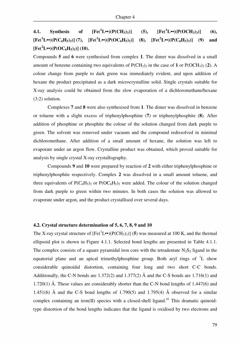
Chapter 4
79
4.1. Synthesis of [Fe(1L••)(P(CH3)3)] (5), [Fe(
1L••)(P(OCH3)3)] (6),
[Fe(1L••)(P(C6H5)3)] (7), [Fe(
1L••)(P(OC6H5)3)] (8), [Fe(
2L••)(P(C6H5)3)] (9) and
[Fe(2L••)(P(OC6H5)3)] (10).
Compounds 5 and 6 were synthesised from complex 1. The dimer was dissolved in a small
amount of benzene containing two equivalents of P(CH3)3 in the case of 1 or P(OCH3)3 (2). A
colour change from purple to dark green was immediately evident, and upon addition of
hexane the product precipitated as a dark microcrystalline solid. Single crystals suitable for
X-ray analysis could be obtained from the slow evaporation of a dichloromethane/hexane
(3:2) solution.
Complexes 7 and 8 were also synthesised from 1. The dimer was dissolved in benzene
or toluene with a slight excess of triphenylphosphine (7) or triphenylphosphite (8). After
addition of phosphine or phosphite the colour of the solution changed from dark purple to
green. The solvent was removed under vacuum and the compound redissolved in minimal
dichloromethane. After addition of a small amount of hexane, the solution was left to
evaporate under an argon flow. Crystalline product was obtained, which proved suitable for
analysis by single crystal X-ray crystallography.
Compounds 9 and 10 were prepared by reaction of 2 with either triphenylphosphine or
triphenylphosphite respectively. Complex 2 was dissolved in a small amount toluene, and
three equivalents of P(C6H5)3 or P(OC6H5)3 were added. The colour of the solution changed
from dark purple to green within two minutes. In both cases the solution was allowed to
evaporate under argon, and the product crystallised over several days.
4.2. Crystal structure determination of 5, 6, 7, 8, 9 and 10
The X-ray crystal structure of [Fe(1L••)(P(CH3)3)] (5) was measured at 100 K, and the thermal
ellipsoid plot is shown in Figure 4.1.1. Selected bond lengths are presented in Table 4.1.1.
The complex consists of a square pyramidal iron core with the tetradentate N2S2 ligand in the
equatorial plane and an apical trimethylphosphine group. Both aryl rings of 1L show
considerable quinoidal distortion, containing four long and two short C-C bonds.
Additionally, the C-N bonds are 1.372(2) and 1.377(2) Å and the C-S bonds are 1.716(1) and
1.720(1) Å. These values are considerably shorter than the C-N bond lengths of 1.447(6) and
1.451(6) Å and the C-S bond lengths of 1.790(5) and 1.795(4) Å observed for a similar
complex containing an iron(II) species with a closed-shell ligand.41 This dramatic quinoid-
type distortion of the bond lengths indicates that the ligand is oxidised by two electrons and
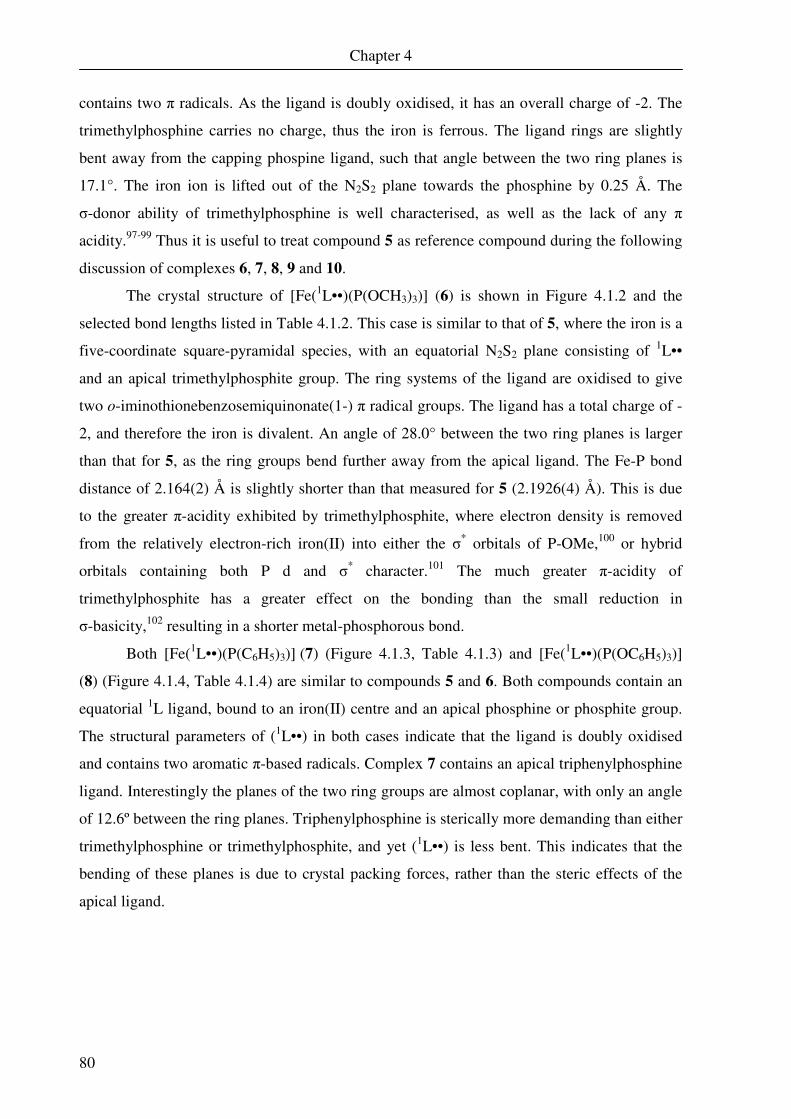
Chapter 4
80
contains two π radicals. As the ligand is doubly oxidised, it has an overall charge of -2. The
trimethylphosphine carries no charge, thus the iron is ferrous. The ligand rings are slightly
bent away from the capping phospine ligand, such that angle between the two ring planes is
17.1°. The iron ion is lifted out of the N2S2 plane towards the phosphine by 0.25 Å. The
σ-donor ability of trimethylphosphine is well characterised, as well as the lack of any π
acidity.97-99 Thus it is useful to treat compound 5 as reference compound during the following
discussion of complexes 6, 7, 8, 9 and 10.
The crystal structure of [Fe(1L••)(P(OCH3)3)] (6) is shown in Figure 4.1.2 and the
selected bond lengths listed in Table 4.1.2. This case is similar to that of 5, where the iron is a
five-coordinate square-pyramidal species, with an equatorial N2S2 plane consisting of 1L••
and an apical trimethylphosphite group. The ring systems of the ligand are oxidised to give
two o-iminothionebenzosemiquinonate(1-) π radical groups. The ligand has a total charge of -
2, and therefore the iron is divalent. An angle of 28.0° between the two ring planes is larger
than that for 5, as the ring groups bend further away from the apical ligand. The Fe-P bond
distance of 2.164(2) Å is slightly shorter than that measured for 5 (2.1926(4) Å). This is due
to the greater π-acidity exhibited by trimethylphosphite, where electron density is removed
from the relatively electron-rich iron(II) into either the σ* orbitals of P-OMe,100 or hybrid
orbitals containing both P d and σ* character.101 The much greater π-acidity of
trimethylphosphite has a greater effect on the bonding than the small reduction in
σ-basicity,102 resulting in a shorter metal-phosphorous bond.
Both [Fe(1L••)(P(C6H5)3)] (7) (Figure 4.1.3, Table 4.1.3) and [Fe(1L••)(P(OC6H5)3)]
(8) (Figure 4.1.4, Table 4.1.4) are similar to compounds 5 and 6. Both compounds contain an
equatorial 1L ligand, bound to an iron(II) centre and an apical phosphine or phosphite group.
The structural parameters of (1L••) in both cases indicate that the ligand is doubly oxidised
and contains two aromatic π-based radicals. Complex 7 contains an apical triphenylphosphine
ligand. Interestingly the planes of the two ring groups are almost coplanar, with only an angle
of 12.6º between the ring planes. Triphenylphosphine is sterically more demanding than either
trimethylphosphine or trimethylphosphite, and yet (1L••) is less bent. This indicates that the
bending of these planes is due to crystal packing forces, rather than the steric effects of the
apical ligand.

Chapter 4
81
Figure 4.2.1. X-Ray crystal structure of 5 (50% probability
ellipsoids).
Table 4.2.1. Bond lengths [Å] of 5
Fe(1) – S(1) 2.1871(4) N(8) – C(9) 1.4695(17)
Fe(1) – S(19) 2.1885(4) C(9) – C(10) 1.5129(17)
Fe(1) – P(20) 2.1926(4) C(10) – C(11) 1.513(2)
Fe(1) – N(8) 1.9000(11) C(11) – N(12) 1.4931(17)
Fe(1) – N(12) 1.8931(11) N(12) – C(13) 1.3765(17)
S(1) – C(2) 1.7156(14) C(13) – C(18) 1.4249(18)
C(2) – C(3) 1.4121(19) C(13) – C(14) 1.4260(18)
C(2) – C(7) 1.4205(18) C(14) – C(15) 1.376(2)
C(3) – C(4) 1.379(2) C(15) – C(16) 1.412(2)
C(4) –C(5) 1.408(2) C(16) – C(17) 1.379(2)
C(5) – C(6) 1.381(2) C(17) – C(18) 1.4072(19)
C(6) – C(7) 1.4273(19) C(18) – S(19) 1.7197(14)
C(7) – N(8) 1.3724(17)
Fe(1)
C(11)
S(1)
S(19)
C(18) C(17)
C(16)
C(15) C(14)
C(13)
N(12)
C(10) C(9)
N(8)
C(7)
C(6)
C(5)
C(4)
C(3) C(2)
P(20)

Chapter 4
82
Figure 4.2.2. X-Ray crystal structure of 6 (50%
probability ellipsoids).
Table 4.2.2. Bond lengths [Å] of 6
Fe(1) – S(1) 2.1876(4) N(8) – C(9) 1.4695(17)
Fe(1) – S(19) 2.1881(4) C(9) – C(10) 1.512(2)
Fe(1) – P(20) 2.164(2) C(10) – C(11) 1.512(2)
Fe(1) – N(8) 1.9029(13) C(11) – N(12) 1.4759(19)
Fe(1) – N(12) 1.9011(12) N(12) – C(13) 1.3701(19)
S(1) – C(2) 1.7166(16) C(13) – C(18) 1.425(2)
C(2) – C(3) 1.412(2) C(13) – C(14) 1.425(2)
C(2) – C(7) 1.423(2) C(14) – C(15) 1.376(2)
C(3) – C(4) 1.381(2) C(15) – C(16) 1.406(2)
C(4) –C(5) 1.404(3) C(16) – C(17) 1.379(2)
C(5) – C(6) 1.379(2) C(17) – C(18) 1.413(2)
C(6) – C(7) 1.433(2) C(18) – S(19) 1.7134(15)
C(7) – N(8) 1.371(2)
Fe(1)
S(1) S(19)
C(18) C(17)
C(16)
C(15)
C(14)
C(13)
N(12)
C(10) C(9)
N(8)
C(7)
C(6) C(5)
C(4)
C(3) C(2)
P(20)

Chapter 4
83
Figure 4.2.3. X-Ray crystal structure of 7 (50%
probability ellipsoids).
Table 4.2.3. Bond lengths [Å] of 7
Fe(1) – S(1) 2.1953(9) N(8) – C(9) 1.478(4)
Fe(1) – S(19) 2.1876(9) C(9) – C(10) 1.495(4)
Fe(1) – P(20) 2.2289(9) C(10) – C(11) 1.495(4)
Fe(1) – N(8) 1.899(2) C(11) – N(12) 1.463(4)
Fe(1) – N(12) 1.905(2) N(12) – C(13) 1.374(4)
S(1) – C(2) 1.709(3) C(13) – C(18) 1.411(4)
C(2) – C(3) 1.400(4) C(13) – C(14) 1.427(4)
C(2) – C(7) 1.420(4) C(14) – C(15) 1.380(5)
C(3) – C(4) 1.372(4) C(15) – C(16) 1.401(5)
C(4) –C(5) 1.409(5) C(16) – C(17) 1.367(5)
C(5) – C(6) 1.364(5) C(17) – C(18) 1.409(4)
C(6) – C(7) 1.420(4) C(18) – S(19) 1.717(3)
C(7) – N(8) 1.372(4)
Fe(1)
S(1) S(19)
C(18) C(17)
C(16)
C(15) C(14)
C(13)
N(12)
C(10) C(9)
N(8)
C(7)
C(6) C(5)
C(4) C(3) C(2)
P(20)
C(11)
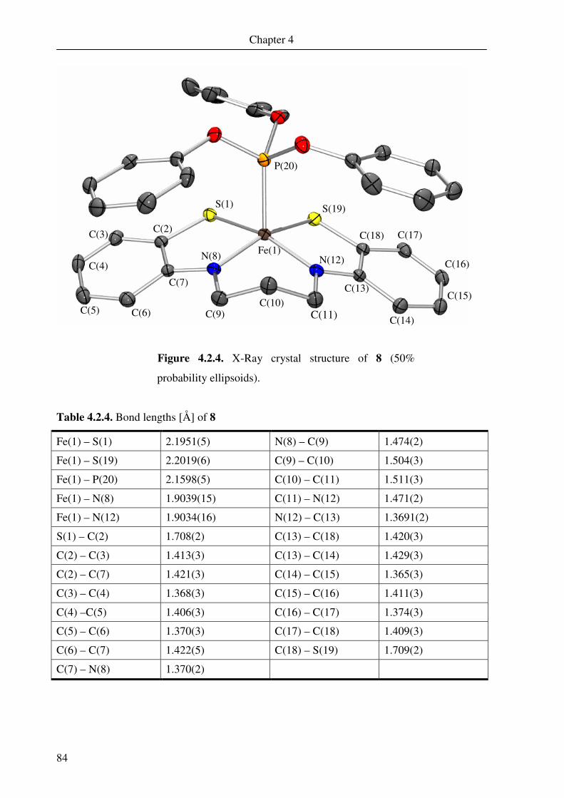
Chapter 4
84
Figure 4.2.4. X-Ray crystal structure of 8 (50%
probability ellipsoids).
Table 4.2.4. Bond lengths [Å] of 8
Fe(1) – S(1) 2.1951(5) N(8) – C(9) 1.474(2)
Fe(1) – S(19) 2.2019(6) C(9) – C(10) 1.504(3)
Fe(1) – P(20) 2.1598(5) C(10) – C(11) 1.511(3)
Fe(1) – N(8) 1.9039(15) C(11) – N(12) 1.471(2)
Fe(1) – N(12) 1.9034(16) N(12) – C(13) 1.3691(2)
S(1) – C(2) 1.708(2) C(13) – C(18) 1.420(3)
C(2) – C(3) 1.413(3) C(13) – C(14) 1.429(3)
C(2) – C(7) 1.421(3) C(14) – C(15) 1.365(3)
C(3) – C(4) 1.368(3) C(15) – C(16) 1.411(3)
C(4) –C(5) 1.406(3) C(16) – C(17) 1.374(3)
C(5) – C(6) 1.370(3) C(17) – C(18) 1.409(3)
C(6) – C(7) 1.422(5) C(18) – S(19) 1.709(2)
C(7) – N(8) 1.370(2)
Fe(1)
C(11)
S(1) S(19)
C(18) C(17)
C(16)
C(15)
C(14)
C(13)
N(12)
C(10) C(9)
N(8)
C(7)
C(6) C(5)
C(4)
C(3) C(2)
P(20)
Chapter 4
85
Complex 7 contains an Fe-P bond slightly longer than that of 5, at 2.2289(9) Å. The
lengthening of this bond implies a weaker interaction between the iron and the phosphorous
centres. It has previously been noted that triphenylphosphine is a weaker σ-donor than
trimethylphosphine, and also a weaker π-acceptor than trimethylphosphite.103 Thus a weaker
bond results between the phosphorous and iron.
The crystal structure of 8, as well as showing showing the same ligand distortion as 7,
also contains an angle between the two ring planes of 31.8°. The phosphorous iron bond was
found to be 2.1598(5) Å, the considerable shortening of which is due to the larger π-acidity of
the triphenylphosphite ligand.
Compounds [Fe(2L••)(P(C6H5)3)] (9) and[Fe(2L••)(P(OC6H5)3)] (10) could also be
crystallised, and the crystal structures of the two complexes were found to be similar. The
quality of the crystal structure measured for 9 was of a lower quality than those previously
mentioned, with 3σ values of up to 24 pm. Although the structure was of a lower quality, this
did not preclude the identification of semi-quinoidal distortion in both ring moieties. The
bridging ethylene group was also found to contain only single C-C and C-N bonds, ruling out
the presence of a “gma” type ligand.104 This evidence led to the classification of the ligand as
a tetradentate dianionic species containing two ligand π radicals, as observed previously for 5
– 8. Therefore the iron must have an oxidation state of +2, also in common with the
previously discussed compounds. The iron phosphorous bond is similar in length to that of 7
at 2.2351(19) Å.
Correspondingly, 10 is also shown to consist of an iron(II) centre bound equatorially
to 2L, which contains two ligand-based π radicals. Triphenylphosphite binds to an apical
position, giving a structure with square-pyramidal geometry. The observed Fe-P bond length
of 2.1302(8) Å is comparable to that seen in complex 8, and is shorter due to the greater
π-acidity of the phosphite ligand.
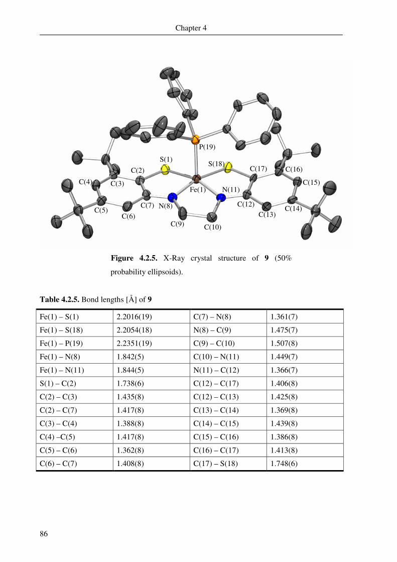
Chapter 4
86
Figure 4.2.5. X-Ray crystal structure of 9 (50%
probability ellipsoids).
Table 4.2.5. Bond lengths [Å] of 9
Fe(1) – S(1) 2.2016(19) C(7) – N(8) 1.361(7)
Fe(1) – S(18) 2.2054(18) N(8) – C(9) 1.475(7)
Fe(1) – P(19) 2.2351(19) C(9) – C(10) 1.507(8)
Fe(1) – N(8) 1.842(5) C(10) – N(11) 1.449(7)
Fe(1) – N(11) 1.844(5) N(11) – C(12) 1.366(7)
S(1) – C(2) 1.738(6) C(12) – C(17) 1.406(8)
C(2) – C(3) 1.435(8) C(12) – C(13) 1.425(8)
C(2) – C(7) 1.417(8) C(13) – C(14) 1.369(8)
C(3) – C(4) 1.388(8) C(14) – C(15) 1.439(8)
C(4) –C(5) 1.417(8) C(15) – C(16) 1.386(8)
C(5) – C(6) 1.362(8) C(16) – C(17) 1.413(8)
C(6) – C(7) 1.408(8) C(17) – S(18) 1.748(6)
Fe(1)
S(1) S(18)
C(17) C(16)
C(15)
C(14) C(13)
C(12)
N(11)
C(10) C(9)
N(8) C(7)
C(6) C(5)
C(4) C(3)
C(2)
P(19)
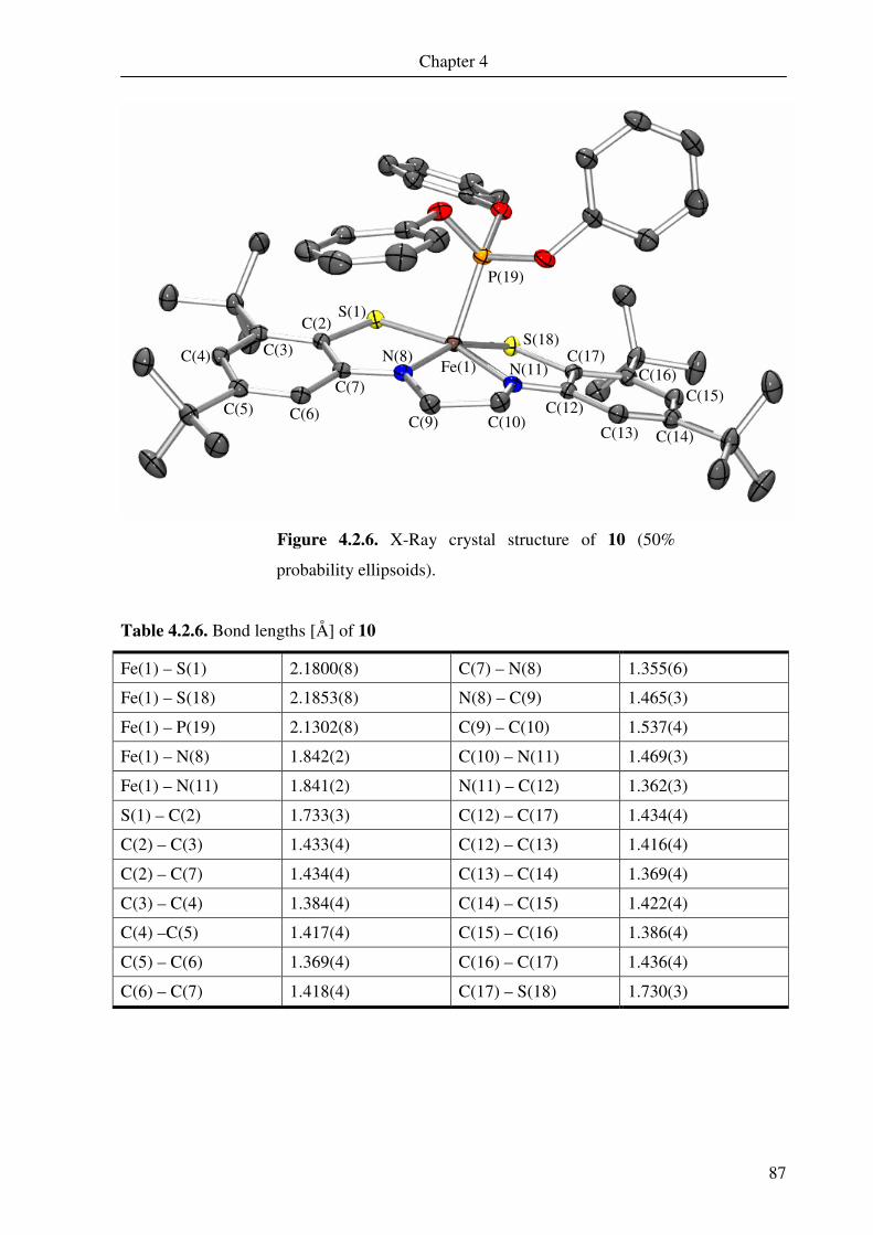
Chapter 4
87
Figure 4.2.6. X-Ray crystal structure of 10 (50%
probability ellipsoids).
Table 4.2.6. Bond lengths [Å] of 10
Fe(1) – S(1) 2.1800(8) C(7) – N(8) 1.355(6)
Fe(1) – S(18) 2.1853(8) N(8) – C(9) 1.465(3)
Fe(1) – P(19) 2.1302(8) C(9) – C(10) 1.537(4)
Fe(1) – N(8) 1.842(2) C(10) – N(11) 1.469(3)
Fe(1) – N(11) 1.841(2) N(11) – C(12) 1.362(3)
S(1) – C(2) 1.733(3) C(12) – C(17) 1.434(4)
C(2) – C(3) 1.433(4) C(12) – C(13) 1.416(4)
C(2) – C(7) 1.434(4) C(13) – C(14) 1.369(4)
C(3) – C(4) 1.384(4) C(14) – C(15) 1.422(4)
C(4) –C(5) 1.417(4) C(15) – C(16) 1.386(4)
C(5) – C(6) 1.369(4) C(16) – C(17) 1.436(4)
C(6) – C(7) 1.418(4) C(17) – S(18) 1.730(3)
Fe(1)
S(1)
S(18) C(17)
C(16) C(15)
C(14) C(13)
C(12)
N(11)
C(10) C(9)
N(8)
C(7)
C(6) C(5)
C(4) C(3)
C(2)
P(19)

Chapter 4
88
4.3 Electronic absorption spectroscopy
The UV-vis spectra of the six complexes 5 – 10 are shown in Figure 4.3.1, and the band
information is summarised in Table 4.3.1.
Figure 4.3.1. Electronic spectra of 5, 6, 7, 8, 9 and 10.
Complexes 9 and 10 were measured in toluene, the remainder
in dichloromethane.
300 400 500 600 700 800 900 1000
0.0
0.5
1.0
1.5
2.0
2.5
3.0
3.5
εε εε / /
/
/ 1
04 M
-1 c
m-1
λλλλ / nm
400 600 800 1000
0.0
0.5
1.0
1.5
2.0
2.5
3.0
3.5
εε εε / /
/
/ 1
04 M
-1 c
m-1
λλλλ / nm
400 600 800 1000
0.0
0.5
1.0
1.5
2.0
εε εε / 1
04 M
-1 c
m-1
λλλλ / nm
400 600 800 1000
0.0
0.5
1.0
1.5
2.0
εε εε / 1
04 M
-1 c
m-1
λλλλ / nm
400 600 800 1000
0.0
0.5
1.0
1.5
2.0
2.5
εε εε / 1
04 M
-1 c
m-1
λλλλ / nm
400 600 800 1000
0.0
0.5
1.0
1.5
2.0
2.5
εε εε / 1
04 M
-1 c
m-1
λλλλ / nm
5 6
7 8
9 10
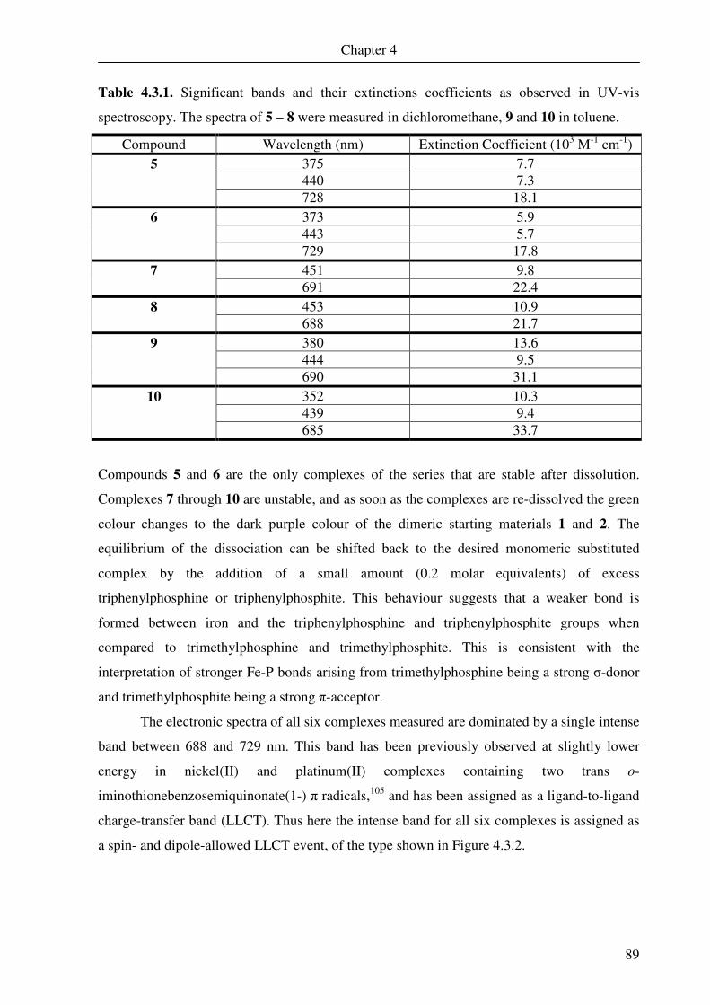
Chapter 4
89
Table 4.3.1. Significant bands and their extinctions coefficients as observed in UV-vis
spectroscopy. The spectra of 5 – 8 were measured in dichloromethane, 9 and 10 in toluene.
Compound Wavelength (nm) Extinction Coefficient (103 M-1 cm-1) 375 7.7 440 7.3
5
728 18.1 373 5.9 443 5.7
6
729 17.8 451 9.8 7
691 22.4 453 10.9 8
688 21.7 380 13.6 444 9.5
9
690 31.1 352 10.3 439 9.4
10
685 33.7
Compounds 5 and 6 are the only complexes of the series that are stable after dissolution.
Complexes 7 through 10 are unstable, and as soon as the complexes are re-dissolved the green
colour changes to the dark purple colour of the dimeric starting materials 1 and 2. The
equilibrium of the dissociation can be shifted back to the desired monomeric substituted
complex by the addition of a small amount (0.2 molar equivalents) of excess
triphenylphosphine or triphenylphosphite. This behaviour suggests that a weaker bond is
formed between iron and the triphenylphosphine and triphenylphosphite groups when
compared to trimethylphosphine and trimethylphosphite. This is consistent with the
interpretation of stronger Fe-P bonds arising from trimethylphosphine being a strong σ-donor
and trimethylphosphite being a strong π-acceptor.
The electronic spectra of all six complexes measured are dominated by a single intense
band between 688 and 729 nm. This band has been previously observed at slightly lower
energy in nickel(II) and platinum(II) complexes containing two trans o-
iminothionebenzosemiquinonate(1-) π radicals,105 and has been assigned as a ligand-to-ligand
charge-transfer band (LLCT). Thus here the intense band for all six complexes is assigned as
a spin- and dipole-allowed LLCT event, of the type shown in Figure 4.3.2.
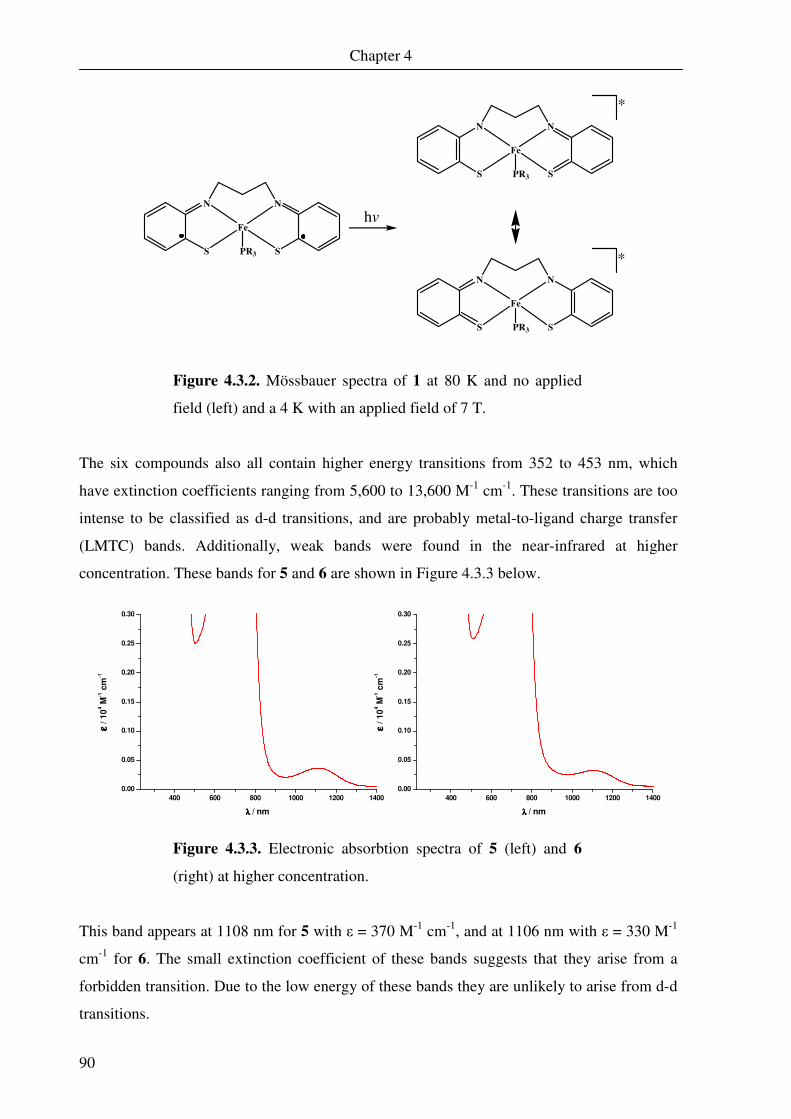
Chapter 4
90
N
S
N
S
Fe
PR3
N
S
N
S
Fe
PR3
N
S
N
S
Fe
PR3
Figure 4.3.2. Mössbauer spectra of 1 at 80 K and no applied
field (left) and a 4 K with an applied field of 7 T.
The six compounds also all contain higher energy transitions from 352 to 453 nm, which
have extinction coefficients ranging from 5,600 to 13,600 M-1 cm-1. These transitions are too
intense to be classified as d-d transitions, and are probably metal-to-ligand charge transfer
(LMTC) bands. Additionally, weak bands were found in the near-infrared at higher
concentration. These bands for 5 and 6 are shown in Figure 4.3.3 below.
Figure 4.3.3. Electronic absorbtion spectra of 5 (left) and 6
(right) at higher concentration.
This band appears at 1108 nm for 5 with ε = 370 M-1 cm-1, and at 1106 nm with ε = 330 M-1
cm-1 for 6. The small extinction coefficient of these bands suggests that they arise from a
forbidden transition. Due to the low energy of these bands they are unlikely to arise from d-d
transitions.
hv
*
*
400 600 800 1000 1200 1400
0.00
0.05
0.10
0.15
0.20
0.25
0.30
εε εε /
10
4 M
-1 c
m-1
λλλλ / nm
400 600 800 1000 1200 1400
0.00
0.05
0.10
0.15
0.20
0.25
0.30
εε εε /
10
4 M
-1 c
m-1
λλλλ / nm
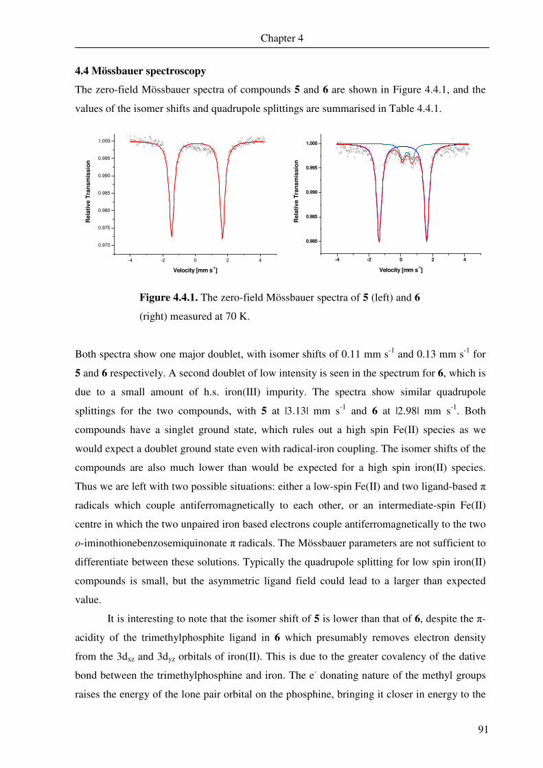
Chapter 4
91
4.4 Mössbauer spectroscopy
The zero-field Mössbauer spectra of compounds 5 and 6 are shown in Figure 4.4.1, and the
values of the isomer shifts and quadrupole splittings are summarised in Table 4.4.1.
Figure 4.4.1. The zero-field Mössbauer spectra of 5 (left) and 6
(right) measured at 70 K.
Both spectra show one major doublet, with isomer shifts of 0.11 mm s-1 and 0.13 mm s-1 for
5 and 6 respectively. A second doublet of low intensity is seen in the spectrum for 6, which is
due to a small amount of h.s. iron(III) impurity. The spectra show similar quadrupole
splittings for the two compounds, with 5 at |3.13| mm s-1 and 6 at |2.98| mm s-1. Both
compounds have a singlet ground state, which rules out a high spin Fe(II) species as we
would expect a doublet ground state even with radical-iron coupling. The isomer shifts of the
compounds are also much lower than would be expected for a high spin iron(II) species.
Thus we are left with two possible situations: either a low-spin Fe(II) and two ligand-based π
radicals which couple antiferromagnetically to each other, or an intermediate-spin Fe(II)
centre in which the two unpaired iron based electrons couple antiferromagnetically to the two
o-iminothionebenzosemiquinonate π radicals. The Mössbauer parameters are not sufficient to
differentiate between these solutions. Typically the quadrupole splitting for low spin iron(II)
compounds is small, but the asymmetric ligand field could lead to a larger than expected
value.
It is interesting to note that the isomer shift of 5 is lower than that of 6, despite the π-
acidity of the trimethylphosphite ligand in 6 which presumably removes electron density
from the 3dxz and 3dyz orbitals of iron(II). This is due to the greater covalency of the dative
bond between the trimethylphosphine and iron. The e- donating nature of the methyl groups
raises the energy of the lone pair orbital on the phosphine, bringing it closer in energy to the
-4 -2 0 2 4
0.980
0.985
0.990
0.995
1.000
Re
lati
ve
Tra
ns
mis
sio
n
Velocity [mm s-1]
-4 -2 0 2 4
0.970
0.975
0.980
0.985
0.990
0.995
1.000
Re
lati
ve
Tra
ns
mis
sio
n
Velocity [mm s-1]
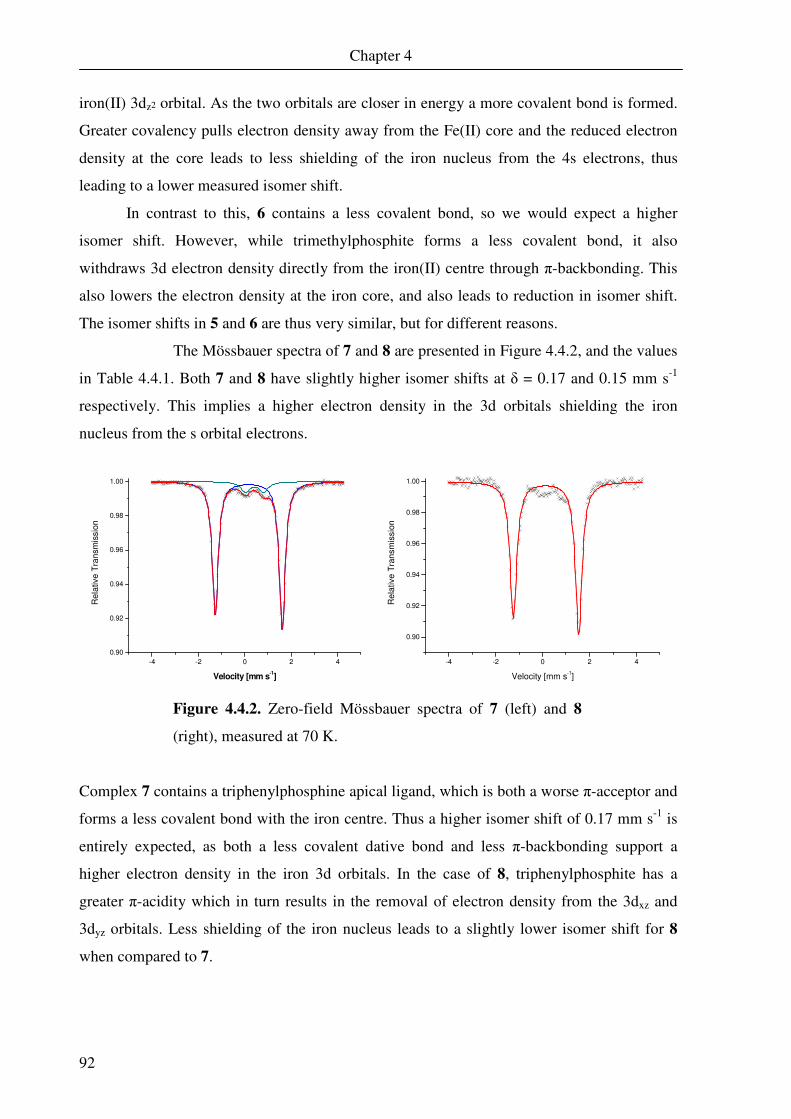
Chapter 4
92
iron(II) 3dz2 orbital. As the two orbitals are closer in energy a more covalent bond is formed.
Greater covalency pulls electron density away from the Fe(II) core and the reduced electron
density at the core leads to less shielding of the iron nucleus from the 4s electrons, thus
leading to a lower measured isomer shift.
In contrast to this, 6 contains a less covalent bond, so we would expect a higher
isomer shift. However, while trimethylphosphite forms a less covalent bond, it also
withdraws 3d electron density directly from the iron(II) centre through π-backbonding. This
also lowers the electron density at the iron core, and also leads to reduction in isomer shift.
The isomer shifts in 5 and 6 are thus very similar, but for different reasons.
The Mössbauer spectra of 7 and 8 are presented in Figure 4.4.2, and the values
in Table 4.4.1. Both 7 and 8 have slightly higher isomer shifts at δ = 0.17 and 0.15 mm s-1
respectively. This implies a higher electron density in the 3d orbitals shielding the iron
nucleus from the s orbital electrons.
Figure 4.4.2. Zero-field Mössbauer spectra of 7 (left) and 8
(right), measured at 70 K.
Complex 7 contains a triphenylphosphine apical ligand, which is both a worse π-acceptor and
forms a less covalent bond with the iron centre. Thus a higher isomer shift of 0.17 mm s-1 is
entirely expected, as both a less covalent dative bond and less π-backbonding support a
higher electron density in the iron 3d orbitals. In the case of 8, triphenylphosphite has a
greater π-acidity which in turn results in the removal of electron density from the 3dxz and
3dyz orbitals. Less shielding of the iron nucleus leads to a slightly lower isomer shift for 8
when compared to 7.
-4 -2 0 2 4
0.90
0.92
0.94
0.96
0.98
1.00
Re
lative
Tra
nsm
issio
n
Velocity [mm s-1]
-4 -2 0 2 4
0.90
0.92
0.94
0.96
0.98
1.00
Re
lative
Tra
nsm
issio
n
Velocity [mm s-1]
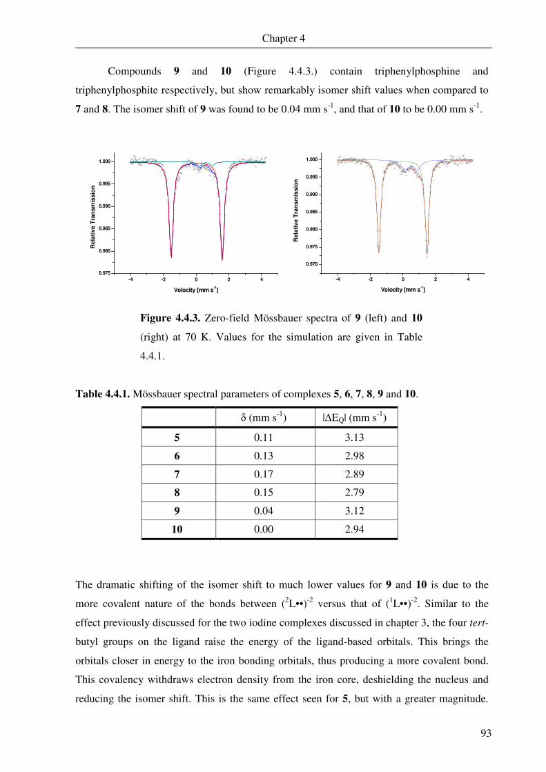
Chapter 4
93
Compounds 9 and 10 (Figure 4.4.3.) contain triphenylphosphine and
triphenylphosphite respectively, but show remarkably isomer shift values when compared to
7 and 8. The isomer shift of 9 was found to be 0.04 mm s-1, and that of 10 to be 0.00 mm s-1.
Figure 4.4.3. Zero-field Mössbauer spectra of 9 (left) and 10
(right) at 70 K. Values for the simulation are given in Table
4.4.1.
Table 4.4.1. Mössbauer spectral parameters of complexes 5, 6, 7, 8, 9 and 10.
δ (mm s-1) |∆EQ| (mm s-1)
5 0.11 3.13
6 0.13 2.98
7 0.17 2.89
8 0.15 2.79
9 0.04 3.12
10 0.00 2.94
The dramatic shifting of the isomer shift to much lower values for 9 and 10 is due to the
more covalent nature of the bonds between (2L••)-2 versus that of (1L••)-2. Similar to the
effect previously discussed for the two iodine complexes discussed in chapter 3, the four tert-
butyl groups on the ligand raise the energy of the ligand-based orbitals. This brings the
orbitals closer in energy to the iron bonding orbitals, thus producing a more covalent bond.
This covalency withdraws electron density from the iron core, deshielding the nucleus and
reducing the isomer shift. This is the same effect seen for 5, but with a greater magnitude.
-4 -2 0 2 4
0.970
0.975
0.980
0.985
0.990
0.995
1.000
Re
lati
ve
Tra
ns
mis
sio
nVelocity [mm s
-1]
-4 -2 0 2 4
0.975
0.980
0.985
0.990
0.995
1.000
Re
lati
ve
Tra
ns
mis
sio
n
Velocity [mm s-1]

Chapter 4
94
The isomer shift of 10 is in turn reduced further due to the propensity of the
triphenylphosphite to remove further electron density from the iron centre.
Applied-field Mössbauer measurements were also made of compounds 9 and 10
with a field strength of 7 T at 4.2 K. Both spectra (presented in Figure 4.4.4) could be
successfully simulated assuming a singlet ground state, confirmed the diamagnetic nature of
this class of compounds.
Figure 4.4.4. Mössbauer spectra of solid 9 (left) and 10 (right),
with an applied field of 7 T and at 4.2 K. Simulation parameters
are given in the text.
The applied-field spectra of 9 could be simulated with St = 0, an isomer shift of 0.04 mm s-1,
a quadrupole splitting of -3.12 mm s-1 and an asymmetry parameter (η) = 0.85. It was found
that the quadrupole splitting of the compound was negative. Little other structural
information could be gleaned, particularly that of the spin state at the iron, due to the
diamagnetic ground state.
4.5 NMR spectroscopy
Proton, carbon and phosphorous NMR at both room- and low-temperature were recorded for
5, 6, 7 and 8 in deuterated dichloromethane and toluene. The numbering scheme for 5 is
provided in Figure 4.5.1.
-15 -10 -5 0 5 10 15
0.995
0.996
0.997
0.998
0.999
1.000
1.001
Re
lati
ve
Tra
ns
mis
sio
n
Velocity [mm s-1]
-15 -10 -5 0 5 10 15
0.988
0.990
0.992
0.994
0.996
0.998
1.000
1.002
Re
lati
ve
Tra
ns
mis
sio
n
Velocity [mm s-1]
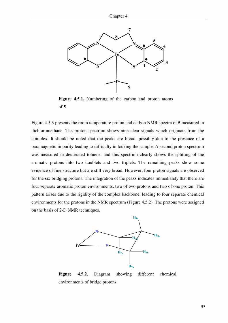
Chapter 4
95
N
S
N
S
Fe
12
3
4
56
7
8
9
P
Figure 4.5.1. Numbering of the carbon and proton atoms
of 5.
Figure 4.5.3 presents the room temperature proton and carbon NMR spectra of 5 measured in
dichloromethane. The proton spectrum shows nine clear signals which originate from the
complex. It should be noted that the peaks are broad, possibly due to the presence of a
paramagnetic impurity leading to difficulty in locking the sample. A second proton spectrum
was measured in deuterated toluene, and this spectrum clearly shows the splitting of the
aromatic protons into two doublets and two triplets. The remaining peaks show some
evidence of fine structure but are still very broad. However, four proton signals are observed
for the six bridging protons. The integration of the peaks indicates immediately that there are
four separate aromatic proton environments, two of two protons and two of one proton. This
pattern arises due to the rigidity of the complex backbone, leading to four separate chemical
environments for the protons in the NMR spectrum (Figure 4.5.2). The protons were assigned
on the basis of 2-D NMR techniques.
N
N
H7a
H7bH7a
H7b
H8a
H8b
Fe
Figure 4.5.2. Diagram showing different chemical
environments of bridge protons.

Chapter 4
96
-0.50.00.51.01.52.02.53.03.54.04.55.05.56.06.57.07.58.08.59.09.510.511.5
0102030405060708090100110120130140150160170180190200210220
Figure 4.5.3. Proton (above) and carbon (below) NMR spectra
of 5 measured at room temperature in CD2Cl2.
CD2Cl2
7b
δ (ppm)
5
2
3
7a
4
8b
8a
9
6
1
5
4
2
7
8
9
δ (ppm)
3

Chapter 4
97
Table 4.5.1. 1H and 13C NMR chemical shifts (ppm) for 5 in CD2Cl2 at 213 and 300 K
213 K 1 2 3 4 5 6
1H ―a d, 7.98,
J= 8 Hz bs, 7.10 bd, 6.78,
J= 4 Hz d, 8.18, J= 8 Hz
―a
13C 167 113 114 122 126 ―b
7a 7b 8a 8b 9
1H s, 4.70 s, 6.55 bs, 2.63 bs, 2.44 s, -0.010 13C 52 37 14
300 K 1 2 3 4 5 6
1H ―a bs, 7.44 bs, 6.99 bs, 6.15 bs, 8.13 ―
a
13C 159 117 117 121 124 160
7a 7b 8a 8b 9
1H bs, 6.82 d, 10.46, J= 5 Hz
bs, 2.17 bs, 2.56 s, -0.34
13C 47 37 14
a) no protons to give signal, b) signal not observed
31P NMR spectroscopy at room temperature gave a broad peak at -126 ppm (free
trimethylphosphine has a peak at -62 ppm).106 This shifted to -55 ppm at 213 K. Typically,
coordinated trimethylphosphine gives 31P NMR peaks much closer to 0 ppm, indicating that
the phosphorous peak is still considerably shifted from archetypal values. Thus the
phosphorous is exposed to some paramagnetic influence. The observed temperature
dependent behaviour rules out the presence of temperature independent paramagnetism
(TIP).
Interestingly, if we examine the proton peaks of the bridging moiety, they are also
shifted considerably from typical values. While a noticeable shift is evident, this is less than
that observed for truly paramagnetic species. Also, when the sample is measured at a lower
temperature, the peaks shift towards more typical values, which is not expected with true
paramagnetic materials. However, as the compound has been characterised as a singlet
diradical species, it is possible that an extremely small population exists in the triplet excited
state, where the two radicals are ferromagnetically coupled. This leads to the proton and
phosphorous NMR signals reflecting the average of the large diamagnetic majority and a
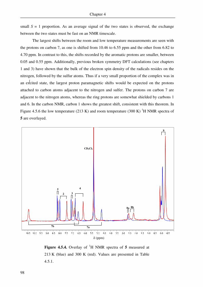
Chapter 4
98
small S = 1 proportion. As an average signal of the two states is observed, the exchange
between the two states must be fast on an NMR timescale.
The largest shifts between the room and low temperature measurements are seen with
the protons on carbon 7, as one is shifted from 10.46 to 6.55 ppm and the other from 6.82 to
4.70 ppm. In contrast to this, the shifts recorded by the aromatic protons are smaller, between
0.05 and 0.55 ppm. Additionally, previous broken symmetry DFT calculations (see chapters
1 and 3) have shown that the bulk of the electron spin density of the radicals resides on the
nitrogen, followed by the sulfur atoms. Thus if a very small proportion of the complex was in
an excited state, the largest proton paramagnetic shifts would be expected on the protons
attached to carbon atoms adjacent to the nitrogen and sulfer. The protons on carbon 7 are
adjacent to the nitrogen atoms, whereas the ring protons are somewhat shielded by carbons 1
and 6. In the carbon NMR, carbon 1 shows the greatest shift, consistent with this theorem. In
Figure 4.5.6 the low temperature (213 K) and room temperature (300 K) 1H NMR spectra of
5 are overlayed.
Figure 4.5.4. Overlay of 1H NMR spectra of 5 measured at
213 K (blue) and 300 K (red). Values are presented in Table
4.5.1.
CD2Cl2
7b
5
2
3
7a
4
8b
8a
9
δ (ppm)
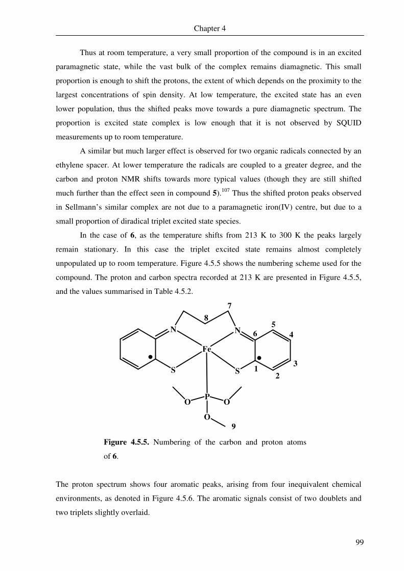
Chapter 4
99
Thus at room temperature, a very small proportion of the compound is in an excited
paramagnetic state, while the vast bulk of the complex remains diamagnetic. This small
proportion is enough to shift the protons, the extent of which depends on the proximity to the
largest concentrations of spin density. At low temperature, the excited state has an even
lower population, thus the shifted peaks move towards a pure diamagnetic spectrum. The
proportion is excited state complex is low enough that it is not observed by SQUID
measurements up to room temperature.
A similar but much larger effect is observed for two organic radicals connected by an
ethylene spacer. At lower temperature the radicals are coupled to a greater degree, and the
carbon and proton NMR shifts towards more typical values (though they are still shifted
much further than the effect seen in compound 5).107 Thus the shifted proton peaks observed
in Sellmann’s similar complex are not due to a paramagnetic iron(IV) centre, but due to a
small proportion of diradical triplet excited state species.
In the case of 6, as the temperature shifts from 213 K to 300 K the peaks largely
remain stationary. In this case the triplet excited state remains almost completely
unpopulated up to room temperature. Figure 4.5.5 shows the numbering scheme used for the
compound. The proton and carbon spectra recorded at 213 K are presented in Figure 4.5.5,
and the values summarised in Table 4.5.2.
N
S
N
S
Fe
12
3
4
56
7
8
9
PO
O
O
Figure 4.5.5. Numbering of the carbon and proton atoms
of 6.
The proton spectrum shows four aromatic peaks, arising from four inequivalent chemical
environments, as denoted in Figure 4.5.6. The aromatic signals consist of two doublets and
two triplets slightly overlaid.
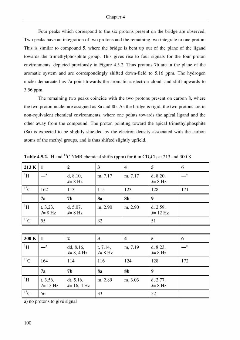
Chapter 4
100
Four peaks which correspond to the six protons present on the bridge are observed.
Two peaks have an integration of two protons and the remaining two integrate to one proton.
This is similar to compound 5, where the bridge is bent up out of the plane of the ligand
towards the trimethylphosphite group. This gives rise to four signals for the four proton
environments, depicted previously in Figure 4.5.2. Thus protons 7b are in the plane of the
aromatic system and are correspondingly shifted down-field to 5.16 ppm. The hydrogen
nuclei demarcated as 7a point towards the aromatic π-electron cloud, and shift upwards to
3.56 ppm.
The remaining two peaks coincide with the two protons present on carbon 8, where
the two proton nuclei are assigned as 8a and 8b. As the bridge is rigid, the two protons are in
non-equivalent chemical environments, where one points towards the apical ligand and the
other away from the compound. The proton pointing toward the apical trimethylphosphite
(8a) is expected to be slightly shielded by the electron density associated with the carbon
atoms of the methyl groups, and is thus shifted slightly upfield.
Table 4.5.2. 1H and 13C NMR chemical shifts (ppm) for 6 in CD2Cl2 at 213 and 300 K
213 K 1 2 3 4 5 6
1H ―a d, 8.10,
J= 8 Hz m, 7.17 m, 7.17 d, 8.20,
J= 8 Hz ―
a
13C 162 113 115 123 128 171
7a 7b 8a 8b 9
1H t, 3.23, J= 8 Hz
d, 5.07, J= 8 Hz
m, 2.90 m, 2.90 d, 2.59, J= 12 Hz
13C 55 32 51
300 K 1 2 3 4 5 6
1H ―a dd, 8.16,
J= 8, 4 Hz t, 7.14, J= 8 Hz
m, 7.19 d, 8.23, J= 8 Hz
―a
13C 164 114 116 124 128 172
7a 7b 8a 8b 9
1H t, 3.56, J= 13 Hz
dt, 5.16, J= 16, 4 Hz
m, 2.89 m, 3.03
d, 2.77, J= 8 Hz
13C 56 33 52
a) no protons to give signal
Chapter 4
101
Again the spectra indicate that the bridging moiety is trapped in one conformation, as there
are separate peaks for the hydrogen nuclei designated in Figure 4.5.2 as 7a, 7b, 8a and 8b.
These peaks are labelled separately in Table 4.5.2. The very small paramagnetic shift
observed indicates that the triplet excited state is populated only very slightly at room
temperature. This is confirmed by no shift observed for the carbon NMR at both
temperatures. The 31P NMR signal shifts from 125 to 133 ppm upon changing the
temperature from 300 to 213 K. The fact that the phosphorous NMR still records some
difference when the proton and carbon NMR spectra do not suggests that the phosphorous
NMR may be a more sensitive probe of excited state population.
The complex also shows no sign of degradation in solution, in contrast to compounds
7 and 8. The implication of this decreased lability of the phosphine is that the
trimethylphosphite-iron bond is stronger than that of trimethylphosphine-iron. This is
consistent with the results obtained from Mössbauer spectroscopy and probably arises due to
the dramatically increased π-acidity of trimethylphosphite, allowing extensive back-bonding
from the electron rich Fe(II) centre.
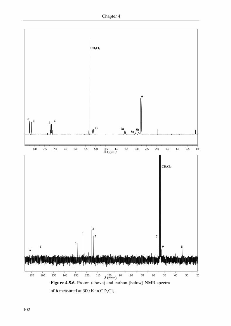
Chapter 4
102
0.00.51.01.52.02.53.03.54.04.55.05.56.06.57.07.58.0
2030405060708090100110120130140150160170
Figure 4.5.6. Proton (above) and carbon (below) NMR spectra
of 6 measured at 300 K in CD2Cl2.
CD2Cl2
5
2
3
7b
7a
8a
9
6
1
5
4
3
2
7
9
8
δ (ppm)
δ (ppm)
4
8b
CD2Cl2

Chapter 4
103
The numbering scheme for 7 is shown in Figure 4.5.7, and the proton and carbon NMR in
Figure 4.5.8.
N
S
N
S
Fe
12
3
4
56
7
8
P
Figure 4.5.7. Numbering scheme for 7.
The proton and carbon NMR spectra of 7 are somewhat more complicated than those
previously discussed, as 7 alone is not stable in solution. Addition of extra
triphenylphosphine is necessary in order to prevent dissociation of triphenylphosphine.
Therefore the dominant feature of the room temperature proton NMR spectrum is an intense,
broad peak at 7.34 ppm. This signal arises from the aromatic protons on the unbound
triphenylphosphine, and is composed of the three expected aromatic multiplets. Protons 5 and
2 could be located downfield of this multiplet, while 3 and 4 could be located within the
multiplet.
The protons on the bridging moiety show a similar pattern to those of 5 and 6, with
four peaks present for the six protons. These peaks show a large amount of shifting at room
temperature. The peak for 7b appears at 8.31 ppm, and that of 7a at 5.78 ppm. These
dramatic shifts probably arise from the same effect as observed in 5, that is a small
population of a triplet excited state, which is not observed in SQUID measurements. Peaks
for 8a and 8b appear at 2.42 and 2.29 ppm respectively. The room temperature 31P NMR
spectrum shows one broad singlet at -5.01 ppm, which accounts for both bound and unbound
phosphine. This indicates that the exchange of the phosphine ligand is rapid on an NMR
timescale, and only an average peak of the two chemical environments is seen.

Chapter 4
104
0.51.01.52.02.53.03.54.04.55.05.56.06.57.07.58.08.5
102030405060708090100110120130140150160170
Figure 4.5.8. Proton NMR spectrum measured at 300 K
(above) and carbon NMR spectrum measured at 223K (below)
of 7 in CD2Cl2.
δ (ppm)
CD2Cl2
5
2
7b
7a
8b
8a
Hexane Diethylether
δ (ppm)
6
1
5
4
3
2
7
8
CD2Cl2
-Ph
4
3
THF
THF
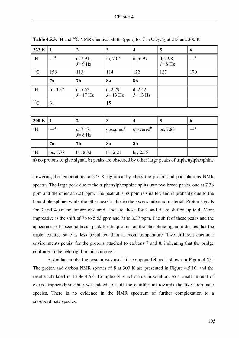
Chapter 4
105
Table 4.5.3. 1H and 13C NMR chemical shifts (ppm) for 7 in CD2Cl2 at 213 and 300 K
223 K 1 2 3 4 5 6
1H ―a d, 7.91,
J= 9 Hz m, 7.04 m, 6.97 d, 7.98
J= 8 Hz ―
a
13C 158 113 114 122 127 170
7a 7b 8a 8b
1H m, 3.37 d, 5.53, J= 17 Hz
d, 2.29, J= 13 Hz
d, 2.42, J= 13 Hz
13C 31 15
300 K 1 2 3 4 5 6
1H ―a d, 7.47,
J= 8 Hz obscuredb obscuredb bs, 7.83 ―
a
7a 7b 8a 8b
1H bs, 5.78 bs, 8.32 bs, 2.21 bs, 2.55
a) no protons to give signal, b) peaks are obscured by other large peaks of triphenylphosphine
Lowering the temperature to 223 K significantly alters the proton and phosphorous NMR
spectra. The large peak due to the triphenylphosphine splits into two broad peaks, one at 7.38
ppm and the other at 7.21 ppm. The peak at 7.38 ppm is smaller, and is probably due to the
bound phosphine, while the other peak is due to the excess unbound material. Proton signals
for 3 and 4 are no longer obscured, and are those for 2 and 5 are shifted upfield. More
impressive is the shift of 7b to 5.53 ppm and 7a to 3.37 ppm. The shift of these peaks and the
appearance of a second broad peak for the protons on the phosphine ligand indicates that the
triplet excited state is less populated than at room temperature. Two different chemical
environments persist for the protons attached to carbons 7 and 8, indicating that the bridge
continues to be held rigid in this complex.
A similar numbering system was used for compound 8, as is shown in Figure 4.5.9.
The proton and carbon NMR spectra of 8 at 300 K are presented in Figure 4.5.10, and the
results tabulated in Table 4.5.4. Complex 8 is not stable in solution, so a small amount of
excess triphenylphosphite was added to shift the equilibrium towards the five-coordinate
species. There is no evidence in the NMR spectrum of further complexation to a
six-coordinate species.
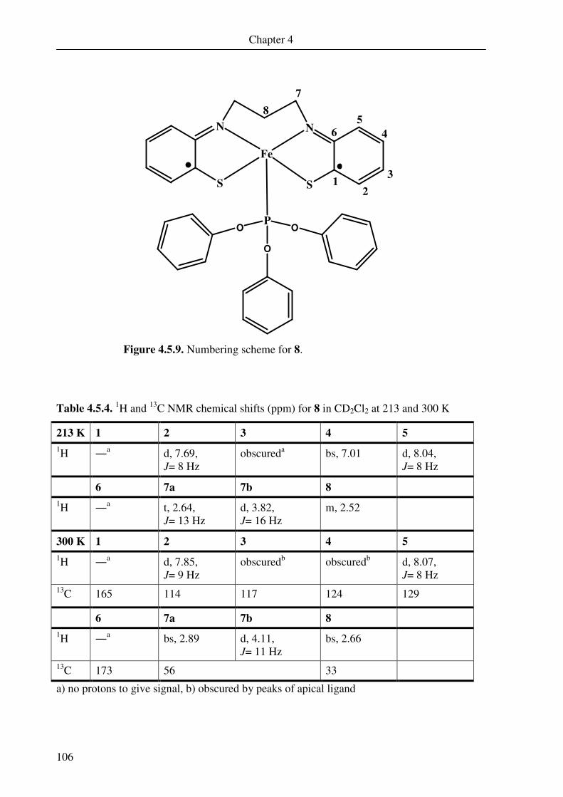
Chapter 4
106
N
S
N
S
Fe
12
3
4
56
7
8
PO
O
O
Figure 4.5.9. Numbering scheme for 8.
Table 4.5.4. 1H and 13C NMR chemical shifts (ppm) for 8 in CD2Cl2 at 213 and 300 K
213 K 1 2 3 4 5
1H ―a d, 7.69,
J= 8 Hz obscureda bs, 7.01 d, 8.04,
J= 8 Hz
6 7a 7b 8
1H ―a t, 2.64,
J= 13 Hz d, 3.82, J= 16 Hz
m, 2.52
300 K 1 2 3 4 5
1H ―a d, 7.85,
J= 9 Hz obscuredb obscuredb d, 8.07,
J= 8 Hz 13C 165 114 117 124 129
6 7a 7b 8
1H ―a bs, 2.89 d, 4.11,
J= 11 Hz bs, 2.66
13C 173 56 33
a) no protons to give signal, b) obscured by peaks of apical ligand

Chapter 4
107
0.51.01.52.02.53.03.54.04.55.05.56.06.57.07.58.0
102030405060708090100110120130140150160170
Figure 4.5.10. Proton NMR spectrum (above) and carbon
NMR spectrum (below) of 8 measured at 300 K in CD2Cl2.
δ (ppm)
δ (ppm)
CD2Cl2
5
2
7b
7a
-OPh
8
CD2Cl2
6
1
7
-OPh
8
5
4
3
2

Chapter 4
108
The room temperature proton spectrum is similar to that of 7, but there are some changes.
The two peaks of protons 5 and 2 are clearly perceptible as two doublets at 8.07 and 7.85
ppm. Unfortunately the peaks of the other two aromatic signals from (1L••) are obscured by
the much larger and broader peaks of the aromatic triphenylphosphite hydrogen nuclei. Four
large signals are observed, which account for both complexed and uncomplexed phosphite
species.
The shift of the bridging protons is much less pronounced than that observed for 7,
and only three peaks are observed. Integration of the peaks indicates that each corresponds to
two protons, therefore the protons on 8 give a single broad signal. Upon cooling to 213 K, the
bridge proton signals shift, with 7b moving from 4.11 to 3.82 ppm, and 7a from 2.89 to 2.64
ppm. The fact that the magnitude of this shift is so much smaller indicates that the triplet
excited state is not as populated as that of 8 when compared to 7. The signals at 7.34, 7.143,
6.90 and 6.46 ppm arising from the aromatic protons on triphenylphosphite in the low
temperature proton NMR spectra are dramatically narrowed, and each is split into two peaks
at low temperature. This is due to the slight difference in chemical shift of the protons
between the bound and unbound triphenylphosphite species.
The 31P NMR spectrum measured at 300 K shows two peaks, one at 129 ppm and one
at 135 ppm. These correspond to the unbound and bound triphenylphosphite respectively. As
two peaks are observed, the implication is that exchange of the phosphite ligand is slow
enough that two separate environments are observed. Thus triphenylphosphite is less labile
than triphenylphosphine. This is probably due to a stronger Fe-P bond existing in 8, due to
the extra π-backbonding from the electron-rich iron(II) centre to the π-acidic phosphorous
species.
Across the NMR spectra of the four compounds discussed, the aromatic protons are
not perturbed to any great extent by the change in axial ligand. This is not true however of
the protons on the bridge of the ligand. It is apparent that the compounds containing either
trimethylphosphine or triphenylphosphine (5 and 7) show the greatest paramagnetic shift of
the bridging protons, while the two phosphite containing complexes (6 and 8) show the least
amount of shifting. The compounds can be ranked according to degree of paramagnetic shift
as 5, 7, 8 and 6, where 5 shows the largest shift and 6 the least. Thus the phosphines promote
population of the paramagnetic triplet state, whereas the phosphites inhibit it.
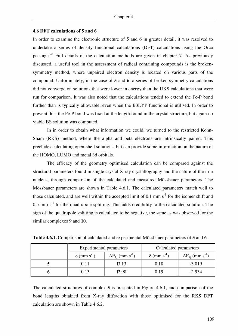
Chapter 4
109
4.6 DFT calculations of 5 and 6
In order to examine the electronic structure of 5 and 6 in greater detail, it was resolved to
undertake a series of density functional calculations (DFT) calculations using the Orca
package.76 Full details of the calculation methods are given in chapter 7. As previously
discussed, a useful tool in the assessment of radical containing compounds is the broken-
symmetry method, where unpaired electron density is located on various parts of the
compound. Unfortunately, in the case of 5 and 6, a series of broken-symmetry calculations
did not converge on solutions that were lower in energy than the UKS calculations that were
run for comparison. It was also noted that the calculations tended to extend the Fe-P bond
further than is typically allowable, even when the B3LYP functional is utilised. In order to
prevent this, the Fe-P bond was fixed at the length found in the crystal structure, but again no
viable BS solution was computed.
In in order to obtain what information we could, we turned to the restricted Kohn-
Sham (RKS) method, where the alpha and beta electrons are intrinsically paired. This
precludes calculating open-shell solutions, but can provide some information on the nature of
the HOMO, LUMO and metal 3d orbitals.
The efficacy of the geometry optimised calculation can be compared against the
structural parameters found in single crystal X-ray crystallography and the nature of the iron
nucleus, through comparison of the calculated and measured Mössbauer parameters. The
Mössbauer parameters are shown in Table 4.6.1. The calculated parameters match well to
those calculated, and are well within the accepted limit of 0.1 mm s-1 for the isomer shift and
0.5 mm s-1 for the quadrupole splitting. This adds credibility to the calculated solution. The
sign of the quadrupole splitting is calculated to be negative, the same as was observed for the
similar complexes 9 and 10.
Table 4.6.1. Comparison of calculated and experimental Mössbauer parameters of 5 and 6.
Experimental parameters Calculated parameters
δ (mm s-1) ∆EQ (mm s-1) δ (mm s-1) ∆EQ (mm s-1)
5 0.11 |3.13| 0.18 -3.019
6 0.13 |2.98| 0.19 -2.934
The calculated structures of complex 5 is presented in Figure 4.6.1, and comparison of the
bond lengths obtained from X-ray diffraction with those optimised for the RKS DFT
calculation are shown in Table 4.6.2.

Chapter 4
110
Figure 4.6.1. Optimised geometry of 5, showing numbering of
the atoms for reference to Table 4.6.2.
The geometry optimised solution compares very well to the bond lengths obtained from
single crystal X-ray diffraction. The bond lengths between the iron centre and the ligands are
somewhat elongated, but this often observed when a B3LYP functional is used. This bond
extension is comparable to that previously observed in this study and elsewhere.43
Figure 4.6.2. Optimised geometry of 6, showing numbering of
the atoms for reference to Table 4.6.3.
The ligand (1L••) shows the classic semi-quinoidal distortion observed when o-
iminothionebenzosemiquinonate radical systems are present. As the calculation is restricted,
C(9)
C(5)
P(20
S(1)
C(7)
C(2) C(3)
C(6)
N(8) N(12)
C(13)
Fe(1)
S(19)
C(4)
C(10) C(11) C(14)
C(15)
C(16)
C(17) C(18)
C(9)
C(5)
P(20
S(1)
C(7)
C(2) C(3)
C(6)
N(8) N(12)
C(13)
Fe(1)
S(19)
C(4)
C(10) C(11) C(14)
C(15)
C(16)
C(17) C(18)

Chapter 4
111
the distortion is not caused by the electron density of individual π radicals, but the electron
density of an electron pair shared across the whole ligand. The aromatic C-S and C-N bonds
are also shorter than expected for a single bond but longer than those of the double bond, as
is expected with the oxidised ligand.
Table 4.6.2. Comparison of bond lengths [Å] between the geometry optimisation of the RKS
DFT calculation and the experimental values obtained from single crystal X-ray
measurements of 5.
Experimental values RKS calculation
Fe(1) – P(20) 2.1926(4) 2.218
Fe(1) – N(8) 1.9000(11) 1.928
Fe(1) – N(12) 1.8931(11) 1.924
Fe(1) – S(1) 2.1871(4) 2.230
Fe(1) – S(19) 2.1885(4) 2.234
S(1) – C(2) 1.7156(14) 1.726
C(2) – C(3) 1.4121(19) 1.413
C(2) – C(7) 1.4205(18) 1.434
C(3) – C(4) 1.379(2) 1.385
C(4) – C(5) 1.408(2) 1.414
C(5) – C(6) 1.381(2) 1.385
C(6) – C(7) 1.4273(19) 1.431
C(7) – N(8) 1.3724(17) 1.369
N(8) – C(9) 1.4695(17) 1.461
C(9) – C(10) 1.5129(17) 1.518
C(10) – C(11) 1.513(2) 1.519
C(11) – N(12) 1.4931(17) 1.462
N(12) – C(13) 1.3765(17) 1.369
C(13) – C(18) 1.4249(18) 1.434
C(13) – C(14) 1.4260(18) 1.431
C(14) – C(15) 1.376(2) 1.385
C(15) – C(16) 1.412(2) 1.413
C(16) – C(17) 1.379(2) 1.385
C(17) – C(18) 1.4072(19) 1.419
C(18) – S(19) 1.7197(14) 1.726
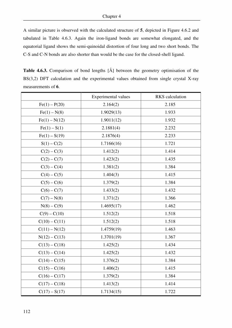
Chapter 4
112
A similar picture is observed with the calculated structure of 5, depicted in Figure 4.6.2 and
tabulated in Table 4.6.3. Again the iron-ligand bonds are somewhat elongated, and the
equatorial ligand shows the semi-quinoidal distortion of four long and two short bonds. The
C-S and C-N bonds are also shorter than would be the case for the closed-shell ligand.
Table 4.6.3. Comparison of bond lengths [Å] between the geometry optimisation of the
BS(3,2) DFT calculation and the experimental values obtained from single crystal X-ray
measurements of 6.
Experimental values RKS calculation
Fe(1) – P(20) 2.164(2) 2.185
Fe(1) – N(8) 1.9029(13) 1.933
Fe(1) – N(12) 1.9011(12) 1.932
Fe(1) – S(1) 2.1881(4) 2.232
Fe(1) – S(19) 2.1876(4) 2.233
S(1) – C(2) 1.7166(16) 1.721
C(2) – C(3) 1.412(2) 1.414
C(2) – C(7) 1.423(2) 1.435
C(3) – C(4) 1.381(2) 1.384
C(4) – C(5) 1.404(3) 1.415
C(5) – C(6) 1.379(2) 1.384
C(6) – C(7) 1.433(2) 1.432
C(7) – N(8) 1.371(2) 1.366
N(8) – C(9) 1.4695(17) 1.462
C(9) – C(10) 1.512(2) 1.518
C(10) – C(11) 1.512(2) 1.518
C(11) – N(12) 1.4759(19) 1.463
N(12) – C(13) 1.3701(19) 1.367
C(13) – C(18) 1.425(2) 1.434
C(13) – C(14) 1.425(2) 1.432
C(14) – C(15) 1.376(2) 1.384
C(15) – C(16) 1.406(2) 1.415
C(16) – C(17) 1.379(2) 1.384
C(17) – C(18) 1.413(2) 1.414
C(17) – S(17) 1.7134(15) 1.722
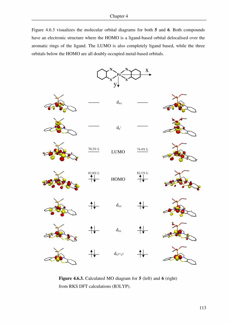
Chapter 4
113
Figure 4.6.3 visualizes the molecular orbital diagrams for both 5 and 6. Both compounds
have an electronic structure where the HOMO is a ligand-based orbital delocalised over the
aromatic rings of the ligand. The LUMO is also completely ligand based, while the three
orbitals below the HOMO are all doubly occupied metal-based orbitals.
N
S
N
S
Fe
Figure 4.6.3. Calculated MO diagram for 5 (left) and 6 (right)
from RKS DFT calculations (B3LYP).
dxy
LUMO
dxz
dyz
dz2
HOMO
dx2-y2
82.1% L 82.8% L
74.4% L 70.2% L
y
x

Chapter 4
114
The coordinate system has been defined in such a way that the x and y axis point between the
equatorial ligand donor atoms, and the z axis lies along the iron-phosphorous bond. This
ensures easily identifiable dxz and dyz orbitals in the calculation, but swaps the positions of
the dx2-y2 and dxy orbitals.
The calculation indicates that the 3dxz, 3dyz and 3dx2-y2 orbitals are all occupied and
the 3dz2 and 3dxy are both empty. The HOMO is almost completely ligand based in both 5
and 6, which is expected. This supports the view that the ligand-based orbitals are the redox
active orbitals. The ligand-based LUMO is consistent with the postulated double oxidation of
(1L)4- to (1L••)2-. The MOs constructed by the calculation also suggest that the iron centre is
low-spin iron(II). This rules out an intermediate spin iron(II), which could also be plausibly
suggested based on the experimental evidence.
115
CHAPTER 5
A Square Pyramidal Complex of Iron
Containing a Tetradentate
bis(o-Iminothionebenzosemiquinonate)
and an Apical tert-Butylpyridine Ligand

116

Chapter 5
117
5.0. Introduction
As has been previously discussed, the ligand 1,2-bis(2-mercapto-3,5-di-tert-
butylaniline)ethane (2LH4) contains two redox active centres in the two o-aminothiophenol
groups, where each can be one electron oxidised to give (2L••)2-. However, the ligand
contains a third redox active site, consisting of the N-C2H4-N bridging group between the
aromatic rings. It is possible to oxidise this bridge by one electron and deprotonate both
carbons to give an α-diiminate(1-) π radical group, as is shown in Figure 5.0.1. This
behaviour has been previously reported, though not completely characterised.59
N
S
N
S
N
S
N
S+e-, +2H+
-e-, -2H+
H HH
H
H
H
R
R R
R R
R R
R
Figure 5.0.1. Scheme showing the one electron oxidation and
double deprotonation of (2L··)2-. R = tert-Butyl groups.
This one electron oxidised and double deprotonated α-diiminate(1-) π radical ligand shown in
Figure 5.0.1 is the reduced form of the glyoxal-bis(2-mercaptoanil)2- (gma) ligand, shown in
Figure 5.0.2. This ligand has a long history in coordination chemistry with metal ions,
including nickel(II),32,108-111 zinc(II),112-114 and iron.56,57,70,115
N
S
N
S
H H
Figure 5.0.2. Glyoxal-bis(2-mercaptoanil)2-
Early work by Stiefel et al.32 and Maki et al.111 with this ligand and complexation with nickel
led to the synthesis of the paramagnetic complex [Ni(gma)]-. A complete description of the
electronic structure was not available at the time, and competing viewpoints were
established. Gray’s group suggested that the singly reduced ligand contained a radical that
was located on the α-diimine bridging linkage,108 whereas Holm’s group promulgated the

Chapter 5
118
view that this was perhaps an overly simplistic description due to significant metal induced
g-value anisotropy in the EPR spectra.111
The first crystal structure of a complex containing gma was published in 1992 by
Sellmann et al.56, who solved the crystal structure of the [Fe(gma)]2 dimer. The compound
was described as consisting of a closed shell (gma)2- ligand coordinated to an iron(II) centre
and this view was later advanced by Karsten et al..57 Several derivatives with an apical
pyridine ligand were synthesised and characterised as containing (gma)2- and an iron(II) core.
In 2003 a report was published by Ghosh et al.70 in which the complexes were
re-synthesised and re-characterised with low temperature X-ray crystallography, magnetic
susceptibility, Mössbauer measurements and DFT calculations. It was found that that the iron
complexes were best described as an iron(III) species coordinated to an open-shell (gma•)3- π
radical. This situation arises through an internal redox process, where the ligand is reduced
by the iron(II). Figure 5.0.3 shows the reduction of (gma)2- to (gma•)3-.
N
S
N
S
N
S
N
S
+e-
-e-
H HH H
Figure 5.0.3. Figure showing the reduction of (gma)2- to (gma•)3-.
Thus the α-diiminate π radical (gma•)3- (or its derivative (2Lgma•)) ligand can be approached
from two directions. One method lies through reduction of (gma)2-, which can occur
intramolecularly depending on the complexed metal species, and the other consists of
oxidation and deprotonation of an α-diamine group, such as that found on (2L••)2-.
Chapter 5
119
5.1. [Fe(2Lgma•)(
t-Bupy)] (11)
Synthesis
Compound 11 was synthesised from 2 through the dissolution of 2 in toluene, and the addition
of a 10 molar excess 4-tert-butylpyridine under argon. Upon exposure to a small amount of
air the solution changed colour from dark purple to reddish-brown. Further evaporation of the
solvent led to crystallisation of the complex, which was obtained in good yield. Single
crystals of 11 suitable for X-ray crystallographic measurements were obtained.
Crystal structure determination of 11
Figure 5.1.1 shows the thermal ellipsoid plot obtained for 11 and selected bond lengths are
shown in Table 5.1.1. The crystal structure of the complex clearly shows it is made up of a
square pyramidal iron centre coordinate to an N2S2 ligand in the equatorial plane, and a 4-tert-
butylpyridine at an apical position. The crystal structure is not of exceptionally good quality,
as shown by the large error (3σ) in the bond lengths. However, the error is not so great that it
precludes further interpretation. Examination of the aromatic rings of the ligand indicates that
there is no ligand-based radical delocalised across the rings. The aromatic C-C bond lengths
are almost all equivalent. Some small distortion does occur, but there is no evidence of the
two short, four long bond pattern expected for the o-benzothionesemiquinonate radical. The
bond lengths between the S atoms and the ring are considerably elongated, further indicating
the lack of a radical species.
However, examination of the bridging moiety indicates some perturbation from the
structure of 2. The N-C bond lengths have decreased from 1.462(0.012) and 1.457(0.012) Å
in the dimer to 1.342(0.021) and 1.353(0.021) Å. Thus we can deduce that the N-C bonds of
the bridge have been oxidised. Interestingly these bond lengths in 11 are too long to be a pure
C-N double bond. The bond between C(9) and C(10) of 1.378(0.021) Å is far too short to be a
C-C single bond. The structural data presented here is very similar to that of previously
characterised gma (glyoxal-bis(2-mercaptoanil) complexes.70,116 Thus the structural
parameters of 11 suggest that we in fact have a trianionic radical (2Lgma•)3- coordinated to a
ferric species. This could only result from an internal redox process combined with further
oxidation and the loss of two protons from the carbon bridge.

Chapter 5
120
Figure 5.1.1. Thermal ellipsoid plot of 11 (50 % probability).
Hydrogen atoms have been omitted except for those located on
the unsaturated bridge.
Table 5.1.1. Bond lengths [Å] of 11
Fe(1) – N(19) 2.062(4) C(7) – N(8) 1.402(6)
Fe(1) – N(8) 1.896(4) N(8) – C(9) 1.342(6)
Fe(1) – N(11) 1.892(4) C(9) – C(10) 1.378(7)
Fe(1) – S(18) 2.2048(14) C(10) – N11) 1.353(6)
Fe(1) – S(1) 2.2076(14) N(11) – C(12) 1.400(6)
S(1) – C(2) 1.777(5) C(12) – C(17) 1.401(7)
C(2) – C(3) 1.415(7) C(12) – C(13) 1.393(7)
C(2) – C(7) 1.412(7) C(13) – C(14) 1.393(7)
C(3) – C(4) 1.387(7) C(14) – C(15) 1.399(7)
C(4) – C(5) 1.384(7) C(15) – C(16) 1.382(7)
C(5) – C(6) 1.402(7) C(16) – C(17) 1.425(7)
C(6) – C(7) 1.392(7) C(17) – S(17) 1.776(5)
S(1) Fe(1)
C(2) C(3)
C(4)
C(5) C(6)
C(7) N(8)
C(9) C(10)
C(12) N(11)
C(13) C(14)
C(15) C(16)
C(17) S(18)
N(19)
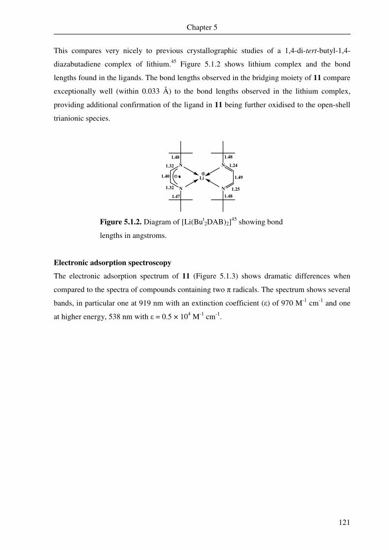
Chapter 5
121
This compares very nicely to previous crystallographic studies of a 1,4-di-tert-butyl-1,4-
diazabutadiene complex of lithium.45 Figure 5.1.2 shows lithium complex and the bond
lengths found in the ligands. The bond lengths observed in the bridging moiety of 11 compare
exceptionally well (within 0.033 Å) to the bond lengths observed in the lithium complex,
providing additional confirmation of the ligand in 11 being further oxidised to the open-shell
trianionic species.
N
N
N
N
Li
1.48
1.32
1.40
1.32
1.47
1.48
1.24
1.49
1.25
1.48
Figure 5.1.2. Diagram of [Li(But2DAB)2]
45 showing bond
lengths in angstroms.
Electronic adsorption spectroscopy
The electronic adsorption spectrum of 11 (Figure 5.1.3) shows dramatic differences when
compared to the spectra of compounds containing two π radicals. The spectrum shows several
bands, in particular one at 919 nm with an extinction coefficient (ε) of 970 M-1 cm-1 and one
at higher energy, 538 nm with ε = 0.5 × 10⁴ M-1 cm-1.

Chapter 5
122
400 600 800 1000 1200 1400 1600
0.0
0.2
0.4
0.6
0.8
1.0
εε εε / 1
04 M
-1 c
m-1
λ / λ / λ / λ / nm
Figure 5.1.3. Electronic spectrum of 11 dissolved in toluene.
It is useful to note the absence of an intense band that would correspond to the LLCT band
previously observed in the ligand diradical complexes.
Magnetic susceptibility
Figure 5.1.4 shows the magnetic moment of 11 at various temperatures and the magnetisation
at various temperatures and field strengths. The magnetic moment of 11 is almost temperature
independent above 50 K with a value of 2.82 µB at 290 K, hence the compound has a triplet
ground state. This triplet ground state arises due to strong antiferromagnetic coupling between
the iron (SFe = 3/2) and a ligand-based radical. The solid lines in Figure 5.1.4 represent spin
Hamiltonian simulations for St = 1. This simulation represents the spin Hamiltonian
simulation for St = 1 based on the following equation:
( ) ( )[ ] SgBSSDESSSDH Byxz ⋅⋅+−++−= µ222 /3/1
Below 40 K the magnetic susceptibility decreases monotonically down to 1.22 µB at 2 K. This
behaviour could be caused by intermolecular coupling or by zero-field splitting (D). In this
case the large distance (> 10 Å) between the iron centres precludes intermolecular
interactions, and the triplet ground state would suggest zero-field splitting as the origin of the
decrease in magnetic moment. This results in the splitting of the triplet ground state into MS =

Chapter 5
123
0 and MS = ± 1 levels, and at lower temperature the population of the MS = 1 state increased.
The measurements could be simulated by taking into account an isotropic g-value of 2.0, a
zero-field splitting of |13.5| cm-1 and a rhombicity (E/D) of 0.27, as well as a small TIP of
250×10-6 emu. Measurement of the magnetisation of the sample at variable temperature and
applied field strengths indicated that the sign of the zero-field splitting was positive.
Figure 5.1.4. Magnetic susceptibility measurements (left) and
magnetisation measurements at variable temperature and
variable field (right) of 11. The experiment could be simulated
(solid lines) with giso = 2, D = +13.47 cm-1, E/D = 0.27, TIP =
250×10-6 emu. This simulation represents the spin Hamiltonian
simulation for St = 1.
From spin projection techniques we can determine the intrinsic zero-field splitting at the iron
using the expression DFe(SFe = 3/2) = 2/3D(St = 1). This gives a value for DFe of 8.98 cm-1. This
fairly large value for D compares well with a similar ferric species, [Fe(N4)I] (where N4 is an
innocent macrocyclic tetradentate ligand), which was found to have D = 13 cm-1.71 The zero-
field splitting for 11 is also close to values of D found for other five-coordinate intermediate-
spin ferric, ferrous and cobalt(III) species.26,27 In these compounds the large zero-field
splitting was found from DFT calculations to arise from spin-orbit coupling, which may be
the case for 11.
Mössbauer spectroscopy
The Mössbauer spectrum of 11 was measured at 80 K, and is shown in Figure 5.1.5. The
isomer shift was found to be 0.247 mm s-1 with a quadrupole splitting of |2.448| mm s-1. These
0 50 100 150 200 250 3001.0
1.2
1.4
1.6
1.8
2.0
2.2
2.4
2.6
2.8
3.0
µµ µµeff [
µµ µµB]
T [K]
-0.2 0.0 0.2 0.4 0.6 0.8 1.0 1.2 1.4 1.6 1.8 2.0 2.2 2.4 2.6
0.00
0.05
0.10
0.15
0.20
0.25
0.30
0.35
0.40
0.45
0.50
0.55
0.60
MM
ol/N
gµµ µµ
B
µµµµBB/kT
7 T
4 T
1 T

Chapter 5
124
parameters are very similar to those found for compounds [Fe(DBMA)py] and
[Fe(GBMA)py] (DBMA is diacetyl-bis-(2-mercaptoanil) and GBMA is glyoxal-bis-(2-
mercaptoanil)) synthesised by Sellmann et al. and Karsten et al. respectively.57,116 Table 5.1.2
compares the Mössbauer values. These values fall within a range where it can be difficult to
assign an oxidation state to the iron. However, extensive studies were carried out on
[Fe(GBMA)py] by Ghosh et al.,70 and it was found that the central iron is best described as
having an intermediate spin state, and is coupled antiferromagnetically to an open-shell
radical trianionic ligand.
Table 5.1.2. Comparison of the Mössbauer parameter of 11, [Fe(GBMA)py]57,116 and
[Fe(GBMA)py].57
δ (mm s-1) ∆EQ (mm s-1)
11 0.247 2.448
[Fe(GBMA)py] 0.29 2.31
[Fe(GBMA)py] 0.28 2.20
-4 -2 0 2 4
0.88
0.90
0.92
0.94
0.96
0.98
1.00
1.02
Re
lati
ve
Tra
nsm
iss
ion
Velocity [mm s-1]
Figure 5.1.5. Zero-field Mössbauer spectrum of 11 measured at
80 K. The simulation (solid line) parameters are δ = 0.247 mm
s-1 and ∆EQ = |2.448| mm s-1.
A series of measurements with an applied field of 7 T with variable temperature were carried
out. No intermolecular interactions were found in the SQUID measurements, so applied field
Mössbauer studies were possible.
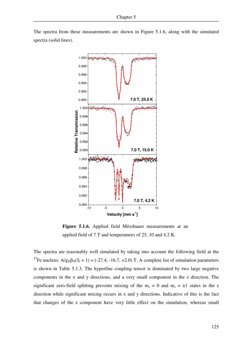
Chapter 5
125
The spectra from these measurements are shown in Figure 5.1.6, along with the simulated
spectra (solid lines).
Figure 5.1.6. Applied field Mössbauer measurements at an
applied field of 7 T and temperatures of 25, 10 and 4.2 K.
The spectra are reasonably well simulated by taking into account the following field at the 57Fe nucleus: A/gNβN(St = 1) = (-27.4, -16.7, +2.0) T. A complete list of simulation parameters
is shown in Table 5.1.3. The hyperfine coupling tensor is dominated by two large negative
components in the x and y directions, and a very small component in the z direction. The
significant zero-field splitting prevents mixing of the ms = 0 and ms = ±1 states in the z
direction while significant mixing occurs in x and y directions. Indicative of this is the fact
that changes of the z component have very little effect on the simulation, whereas small
-10 -5 0 5 100,990
0,992
0,994
0,996
0,998
1,000
7.0 T, 4.2 K
Velocity [mm s-1]
0.990
0.992
0.994
0.996
0.998
1.000
7.0 T, 15.0 K
Re
lati
ve
Tra
ns
mis
sio
n
0.990
0.992
0.994
0.996
0.998
1.000
7.0 T, 25.0 K

Chapter 5
126
adjustments in the x or y directions dramatically alters the pattern and splitting of the
simulation.
Table 5.1.3. Complete list of simulation parameters for 11.
A/gNβN(St = 1)a (-27.4, -16.7, +2.0) T
A/gNβN(SFe = 3/2)a (-18.3, -11.1, +1.3) T
δb 0.247 mm s-1
∆EQc +2.448 mm s-1
ηd 0.2
Dte +13.47 cm-1
E/Df 0.27
Гg 0.3 mm s-1
gISOh 2.0
a) Hyperfine coupling tensor components. b) Isomer shift at 80 K. c) Quadrupole splitting. d)
Asymmetry parameter. e) Zero-field splitting. f) Rhombicity. g) Line width. h) Isotropic g
value.
The A tensor at the 57Fe nucleus can be determined from the hyperfine coupling parameters of
the St = 1 system using spin projection techniques. Together with the isomer shift and
quadrupole splitting, the hyperfine coupling tensor exhibits the classic parameters (two large
negative values and one small positive value) of a five-coordinate intermediate-spin ferric
species. Therefore, the triplet ground state must arise through strong antiferromagnetic
coupling between the iron centre and a ligand-based π radical species.
DFT calculations of 11
The electronic structure of the complex was also examined using DFT calculations,
undertaken with the Orca package.76 Full details of the calculations are specified in chapter 7.
Extensive DFT studies of [M(gma)(X)m]n (M = Zn, Ni, Fe; gma = glyoxal-bis(2-
mercaptoanil); X = py, PH3, CN-, I-; m = 1, 2; n = 0, -1, +1) complexes were undertaken by
Ghosh et al.,70 and the work presented here continues this series of complexes. A broken-
symmetry (BS) approach with the B3LYP functional was utilised, whereby the computational
package assigns unpaired electron density across the molecule based on energetic concerns.
Since a radical is indicated by the spectroscopic data, it is useful to use the BS approach for
11. In order to reduce the computational resources required, a model complex was calculated
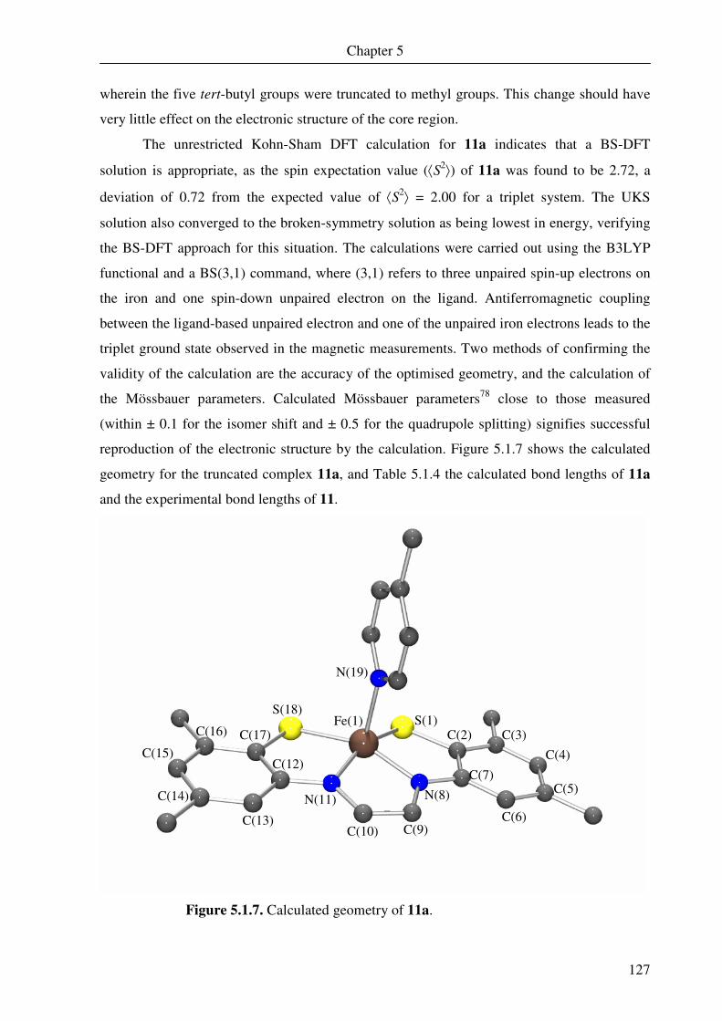
Chapter 5
127
wherein the five tert-butyl groups were truncated to methyl groups. This change should have
very little effect on the electronic structure of the core region.
The unrestricted Kohn-Sham DFT calculation for 11a indicates that a BS-DFT
solution is appropriate, as the spin expectation value (⟨S2⟩) of 11a was found to be 2.72, a
deviation of 0.72 from the expected value of ⟨S2⟩ = 2.00 for a triplet system. The UKS
solution also converged to the broken-symmetry solution as being lowest in energy, verifying
the BS-DFT approach for this situation. The calculations were carried out using the B3LYP
functional and a BS(3,1) command, where (3,1) refers to three unpaired spin-up electrons on
the iron and one spin-down unpaired electron on the ligand. Antiferromagnetic coupling
between the ligand-based unpaired electron and one of the unpaired iron electrons leads to the
triplet ground state observed in the magnetic measurements. Two methods of confirming the
validity of the calculation are the accuracy of the optimised geometry, and the calculation of
the Mössbauer parameters. Calculated Mössbauer parameters78 close to those measured
(within ± 0.1 for the isomer shift and ± 0.5 for the quadrupole splitting) signifies successful
reproduction of the electronic structure by the calculation. Figure 5.1.7 shows the calculated
geometry for the truncated complex 11a, and Table 5.1.4 the calculated bond lengths of 11a
and the experimental bond lengths of 11.
Figure 5.1.7. Calculated geometry of 11a.
Fe(1) S(1) S(18)
N(19)
N(11) N(8)
C(2) C(3)
C(4)
C(5)
C(6)
C(7)
C(9) C(10)
C(12)
C(17) C(16)
C(15)
C(14)
C(13)
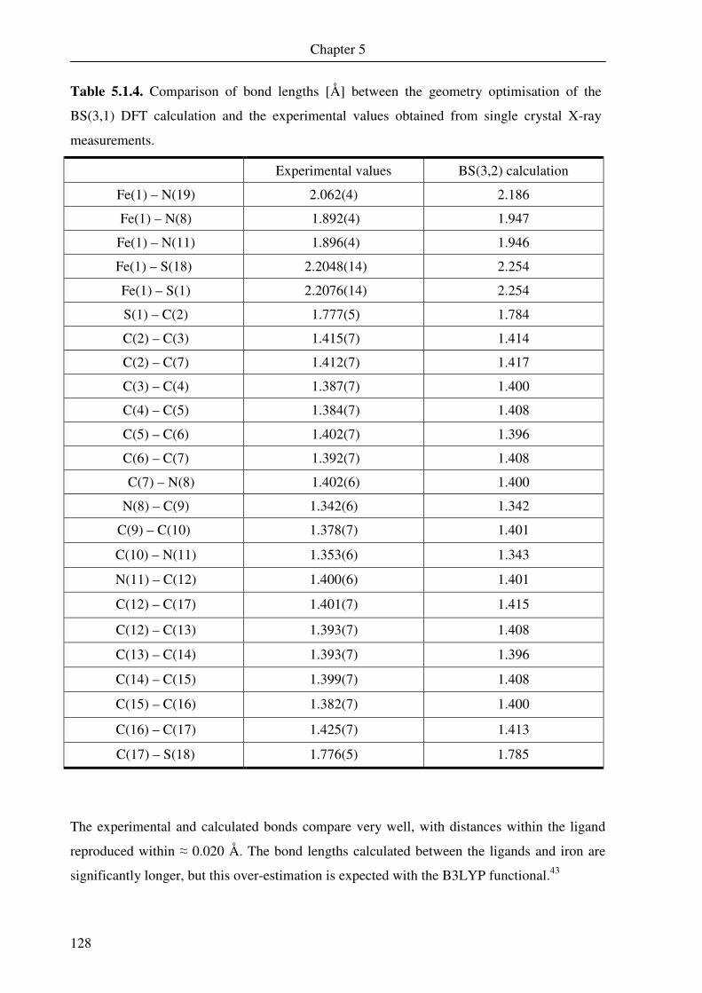
Chapter 5
128
Table 5.1.4. Comparison of bond lengths [Å] between the geometry optimisation of the
BS(3,1) DFT calculation and the experimental values obtained from single crystal X-ray
measurements.
Experimental values BS(3,2) calculation
Fe(1) – N(19) 2.062(4) 2.186
Fe(1) – N(8) 1.892(4) 1.947
Fe(1) – N(11) 1.896(4) 1.946
Fe(1) – S(18) 2.2048(14) 2.254
Fe(1) – S(1) 2.2076(14) 2.254
S(1) – C(2) 1.777(5) 1.784
C(2) – C(3) 1.415(7) 1.414
C(2) – C(7) 1.412(7) 1.417
C(3) – C(4) 1.387(7) 1.400
C(4) – C(5) 1.384(7) 1.408
C(5) – C(6) 1.402(7) 1.396
C(6) – C(7) 1.392(7) 1.408
C(7) – N(8) 1.402(6) 1.400
N(8) – C(9) 1.342(6) 1.342
C(9) – C(10) 1.378(7) 1.401
C(10) – N(11) 1.353(6) 1.343
N(11) – C(12) 1.400(6) 1.401
C(12) – C(17) 1.401(7) 1.415
C(12) – C(13) 1.393(7) 1.408
C(13) – C(14) 1.393(7) 1.396
C(14) – C(15) 1.399(7) 1.408
C(15) – C(16) 1.382(7) 1.400
C(16) – C(17) 1.425(7) 1.413
C(17) – S(18) 1.776(5) 1.785
The experimental and calculated bonds compare very well, with distances within the ligand
reproduced within ≈ 0.020 Å. The bond lengths calculated between the ligands and iron are
significantly longer, but this over-estimation is expected with the B3LYP functional.43

Chapter 5
129
The BS(3,1) DFT calculation of the Mössbauer parameters for 11a give an isomer
shift of 0.287 mm s-1 and a quadrupole splitting of +2.752 mm s-1. This compares extremely
well to the measured results of δ = 0.247 mm s-1 and ∆EQ = +2.448 mm s-1 obtained from the
zero-field and applied-field Mössbauer spectra. This indicates a very good agreement between
the calculated electronic structure and that found by spectroscopic and physical methods.
The calculated Mulliken spin density (Figure 5.1.8) shows an α electron density on the
iron of 2.697 and a ligand-based β spin of 0.806, indicating three unpaired electrons on the
iron and one unpaired electron on the ligand. Over 70% of the ligand-based spin density is
based on the two nitrogen and two carbon atoms, indicating that the radical is strongly
localised on the bridging moiety and that the bridge is oxidised to an α-diiminate(1-) π
radical.
Figure 5.1.8. Mulliken spin density calculated for 11a. Numbers indicate α-
spin density (yellow; positive) and β-spin density (red; negative).
The qualitative MO diagram for the calculation is shown in Figure 5.1.9. The lowest energy
doubly occupied MO is a canonical orbital, while the singly occupied MOs arise from a
corresponding orbital transformation. It is important to note that the axis system is twisted 45°
about the z axis, leading to the dxy and dx2-y2 orbitals swapping position but having no other
effect on the system. This was done to prevent the mixing of the xz and yz orbitals, increasing
clarity of the calculated output. It is useful to examine the corresponding orbitals as they
show most clearly the spin couplings, as the transformed orbitals are arranged so that the spin-
up and spin-down orbitals with the greatest overlap are paired. In this case the spin-up and
+2.697
-0.204
-0.203 -0.117
-0.117
+0.034
-0.082 -0.083
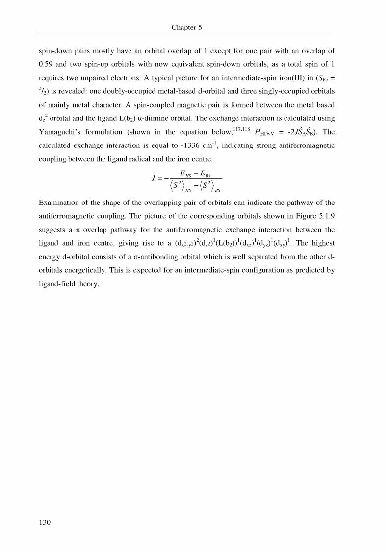
Chapter 5
130
spin-down pairs mostly have an orbital overlap of 1 except for one pair with an overlap of
0.59 and two spin-up orbitals with now equivalent spin-down orbitals, as a total spin of 1
requires two unpaired electrons. A typical picture for an intermediate-spin iron(III) in (SFe = 3/2) is revealed: one doubly-occupied metal-based d-orbital and three singly-occupied orbitals
of mainly metal character. A spin-coupled magnetic pair is formed between the metal based
dz2 orbital and the ligand L(b2) α-diimine orbital. The exchange interaction is calculated using
Yamaguchi’s formulation (shown in the equation below,117,118 ĤHDvV = -2JŜAŜB). The
calculated exchange interaction is equal to -1336 cm-1, indicating strong antiferromagnetic
coupling between the ligand radical and the iron centre.
BSHS
BSHS
SS
EEJ
22 −
−−=
Examination of the shape of the overlapping pair of orbitals can indicate the pathway of the
antiferromagnetic coupling. The picture of the corresponding orbitals shown in Figure 5.1.9
suggests a π overlap pathway for the antiferromagnetic exchange interaction between the
ligand and iron centre, giving rise to a (dx2-y2)2(dz2)1(L(b2))1(dxz)
1(dyz)1(dxy)
1. The highest
energy d-orbital consists of a σ-antibonding orbital which is well separated from the other d-
orbitals energetically. This is expected for an intermediate-spin configuration as predicted by
ligand-field theory.
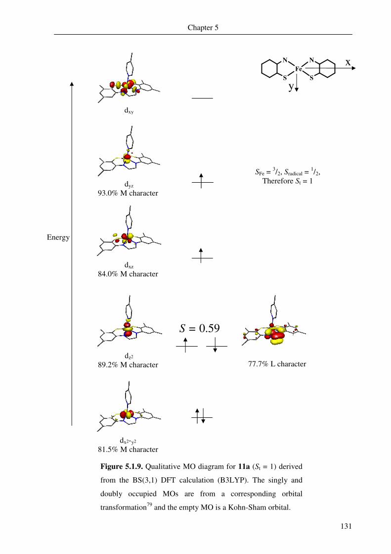
Chapter 5
131
Figure 5.1.9. Qualitative MO diagram for 11a (St = 1) derived
from the BS(3,1) DFT calculation (B3LYP). The singly and
doubly occupied MOs are from a corresponding orbital
transformation79 and the empty MO is a Kohn-Sham orbital.
S = 0.59
dxz 84.0% M character
dyz 93.0% M character
dz2 89.2% M character
dx2-y2 81.5% M character
77.7% L character
dxy
N
S
N
S
Fe
y
x
Energy
SFe = 3/2, Sradical = 1/2, Therefore St = 1

Chapter 5
132

133
CHAPTER 6
Conclusion

134
Chapter 6
135
6.0 Conclusion
All together, eleven complexes have been synthesised in order to examine the properties of
iron complexes containing a tetradentate aminobenzenethiol based ligand. Of particular
interest was the possibility of communication between the two halves of the ligand through a
short bridging spacer. Results have previously been obtained from the ligand 1,2-
ethanediamine-N,N’-bis(2-benzenethiol) (Figure 6.0.1).8,10,11 The carbon bridging moiety is
susceptible to oxidation to the glyoxal-bis(2-mercaptoaniline).
SH
NH HN
HS
Figure 6.0.1. 1,2-ethanediamine-N,N’-bis(2-benzenethiol)
The ligand 1,3-propanediamine-N,N’-bis(2-benzenethiol) (1LH4) (Figure 6.0.2) was chosen
for its three-carbon bridge, which removes the possibility of oxidation to an α-diimine form
and effectively precludes electronic communication through the bridge. In contrast to this, 2LH4 (1,2-bis(2-mercapto-3,5-di-tert-butylaniline)ethane) was chosen for the greater solubility
that the tertiary butyl groups confer.
SH
NH HN
HSSH
NH HN
HS
Figure 6.0.2. 1LH4 (left) and 2LH4 (right).
[Fe(1L•)]2 (1) and [Fe(2L•)]2 (2) were synthesised in order to examine the physical and
electronic structure of the oxidised dimeric species. This class of compounds is not unknown
and previous work conducted by Ghosh et al.11 allows comparison between 1 and 2 and
literature reports. It was found that 1 and 2 have very similar electronic structures, despite
some differences in physical structure.
Both compounds have a dimeric structure, where each monomer is made up of an iron
core bonded equatorially to the tetradentate ligands, 1L for 1 and 2L for 2. The monomers are
bonded through a bridging sulfur group from each ligand, which bonds to the iron of the
Chapter 6
136
opposite subunit. The most obvious difference in the X-ray crystal structures of the two
compounds is the arrangement of the dimer. In 1 the long axes of the two subunits of the
dimer are parallel, while in 2 the long axes are perpendicular. However, this structural
difference has no effect on the electronic structure of the compound. The X-ray crystal
structures also indicate the presence of o-iminothionebenzosemiquinonate π-radicals in the
terminal rings of the ligand. This implies that each ligand has an overall charge of -3, and
therefore each iron centre is must have a charge of +3. The electronic absorption spectra of
the two compounds show characteristic bands which confirm the presence of a ligand-based
π-radical.
Both compounds were found to have a diamagnetic ground state, from applied-field
Mössbauer measurements, and variable-temperature magnetic susceptibility measurements in
the case of 2. Due to coupling between the two centres the elucidation of the spin state at
each iron centre is not trivial, but close examination of the variable-temperature magnetic
moment of 2 allowed some clarification. The two ligand π-radicals couple strongly to the
iron centre, leaving each iron nucleus with an effective doublet spin-state. These in turn
couple strongly to each other with a coupling constant J = -409 cm-1.
The NMR spectra of 2 also showed some interesting shifts, which arise from the
paramagnetism of the compound at higher temperatures. The peaks could be identified using
low-temperature and two-dimensional spectroscopic techniques.
DFT calculations using the B3LYP functional have confirmed the experimental
results. This is the first time DFT calculations have been used to examine the nature of these
dimeric species. The lowest energy solution was found to be a broken symmetry solution,
where two ligand radicals are found in the terminal rings, and both of the iron centres are S = 3/2. The ligand radicals couple to the iron centres through the dxz orbitals, while the singly
occupied dz2 and dyz orbitals of each iron couple antiferromagnetically to the dz2 and dyz of
the other iron centre.
The dimers both reacted with iodine, to give complexes 3 and 4. These complexes
were synthesised to examine the electronic structure of this type of complex, and compare
these to the previously synthesised compounds of Sellmann and Ghosh, where some
confusion had existed about the oxidation states at both the metal and ligand.10,11 It was found
that 3 and 4 have very similar electronic structures, in that both have an intermediate-spin iron
core bound to two ligand-based π radicals which couple to the metal antiferromagnetically.
This was also found to be the case with Ghosh’s and Sellmann’s complexes.11,43 Neither the
tertiary butyl groups nor bridge length between 3, 4, Ghosh’s compound and Sellmann’s
Chapter 6
137
compound alter the spin state, but, as expected, do have a major effect on the solubility of the
compounds. The presence or absence of an unsaturated bridging moiety does not appear to
affect the ground state of the molecule.
Spectroscopic methods have proved vital to the correct elucidation of the metal and
ligand oxidation states, and several of these methods give markers unique to the particular
oxidation state which may be useful in future characterisation of similar complexes. These
include intense ligand-to-ligand charge transfer bands in the electronic spectrum, exhibited in
both 3 and 4, which indicate the presence of a diradical system. Likewise, the unusual
hyperfine coupling pattern that appears at gmin in the EPR spectrum can also be treated as a
marker for the presence of a diradical system where the apical ligand is an iodide or bromide.
For compound 3, single crystals suitable for X-ray crystallographic measurements were
obtained, and the structure was determined which indicated that the ligand was oxidised to
the semi-quinoidal state, due to the appearance of two short and four long C-C bonds.
The spin state of the iron could be explicitly determined for 4 through examination of
the hyperfine coupling tensor A in the applied field Mössbauer measurements. The
occurrence of large negative components (Axx, Ayy) and a small positive z component (Azz)
allow unequivocal assignment of the iron centre as being an intermediate spin ferric species
(SFe = 3/2). Thus, combined with the SQUID measurements indicating an St = ½ ground state,
the applied field Mössbauer spectroscopy provides a powerful indication of the overall
electronic configuration.
DFT calculations utilising the B3LYP functional and taking into account relativistic
effects with ZORA for iodine have been undertaken. These have found that the broken
symmetry solution involving two radicals coupled to a ferric ion is accurate for both 3 and 4,
as has been reported in the case of Sellmann’s and Ghosh’s archetypal complexes.
Six phosphine and phosphite adducts were synthesised, in order to examine the nature
of these complexes. All were synthesised using the dimers 1 or 2 as a starting material, and
upon reaction with trimethylphosphine or phosphite, triphenylphosphine or phosphite, the
five-coordinate compounds 5 – 10 were obtained. Complexes of this nature have previously
been synthesised, most notably by Sellmann et al.119 and Ghosh et al..96 Sellmann had
characterised the compounds as containing a closed-shell ligand bound to an iron(IV) centre,
partially due to misleading magnetic measurements and an apparently paramagnetic proton
NMR spectrum. Ghosh et al. revisited these complexes, and assigned them as iron(II)
complexes containing two ligand-based π radicals. The complexes were found to be
diamagnetic, as the initially paramagnetic magnetic measurements were due to the presence

Chapter 6
138
of a paramagnetic impurity, which could be removed upon repeated crystallisations. The
complexes synthesised here have also been characterised as containing an iron(II) species
bound to a ligand containing two o-iminothinobenzosemiquinonate π radicals. The
complexes containing triphenylphosphine or triphenylphosphite were unstable upon
dissolution, so trimethylphosphine and trimethylphosphite complexes were also synthesised,
due to the stronger binding properties exhibited by these ligands.
Structural determination of all six complexes was possible through the use of low
temperature X-ray diffraction analysis of single crystals. All six were found to be very
similar, and the structural parameters were found to be consistent with an iron(II) centre
bound to ligands (1L) or (2L). In both cases the aromatic systems of the ligands were oxidised
to give (1L••) or (2L••). The bond length of the iron-phosphorous bond is shortest for the
three phosphite complexes; however this is not the best indication of bond strength as the
triphenylphosphite is much more labile than trimethylphosphite.
The electronic absorption spectra of the six complexes are all very similar, with very
intense bands observed between 680 and 730 nm. These have been characterised as ligand-
to-ligand charge transfer bands,105 whose strong intensities can be a marker for complexes
containing two o-iminothinobenzosemiquinonate π radicals in a planar arrangement to one
another. The zero-field Mössbauer spectra are more ambiguous, giving parameters for the
iron nuclei that could arise from several oxidation and spin states. However, the measured
spectra are consistent with an iron(II) low-spin nucleus. The isomer shift also gives
information on the nature of the bond between iron and the phosphines or phosphites, which
is more covalent for trimethylphosphine, and has a large π backbonding component with
triphenylphosphite and trimethylphosphite.
The proton, carbon and phosphorous NMR spectra for complexes 5 – 8 show some
interesting features, which have not previously been characterised. Perhaps most notable are
the paramagnetic shifts observed in the proton NMR for complexes 5 and 7, which could
arise from a very small proportion of populated excited state, in which the ligand radicals are
uncoupled. The large shift of the 31P signal in 5 to more shielded values is very unusual, and
is due to the same effect. A large 31P shift is observed in 6, and it is possible that the
paramagnetic shift of the phosphine nucleus is a useful measure of this effect.
DFT calculations were undertaken on complexes 5 and 6, in order to elucidate the
spin state at the iron(II) centre. Unfortunately broken symmetry calculations converged on a
variety of solutions, remarkably none of which were lower in energy than RKS solutions.
Thus a legitimate broken symmetry solution could not be found. RKS DFT solutions were

Chapter 6
139
examined, and convincingly reproduced experimental structural and Mössbauer parameters.
For both 5 and 6 the HOMO and LUMO were found to be almost completely ligand based.
Complex 11 was obtained from the reaction of 2 with oxygen and 4-tert-
butylpyridine. The electronic structure of 11 could be established using a combination of
spectroscopic, magnetic and physical techniques. The ligand in the complex was
unexpectedly found to have a “gma” type structure, according to the X-ray crystallography.
The C-S and ring-carbon nitrogen bonds are lengthened compared to those of complex 3 and
there is no evidence of quinoidal-type distortion in the aromatic ring, though the modest
quality of the structure precludes strict assignment. Interestingly the N-C bonds of the bridge
are shorter than expected, though not short enough to be pure imine bonds. The C-C bond
length of the bridge is also considerably shorter than that expected for a single bond,
indicating delocalisation across the whole bridging moiety. The similarity of these bond
lengths to those observed in [Li(tBu2DAB)2]45 suggest a π radical in the bridge. In order for
this to occur the complex must be further oxidised by two electrons and undergo two
deprotonations. The reaction mixture, with a large excess of basic tert-butylpyridine and
further exposure to atmospheric oxygen provides the conditions necessary for the oxidation
and electronic rearrangement of the ligand. The oxidation of a presumed precursor (based on
the assignment of oxidation state of the dimer) is shown in Figure 6.0.3.
NR
R
S
N R
R
S
FeIII
N
H
H H
H
NR
R
S
N R
R
S
FeIII
H H
N
R
0 0
-2e-, -2H+
R
11
Figure 6.0.3. Scheme showing the oxidation and deprotonation
of hypothesised reactant to 11. R = tert-butyl.
Compound 11 was found to have a triplet ground state by magnetic susceptibility
measurements. The brisk decrease in µeff at low temperature is attributed to zero-field
splitting because the distance between the molecules in the solid state rules out any

Chapter 6
140
intermolecular interaction. The experimental results could be modelled by taking into
account a zero-field splitting of 13.47 cm-1. Further measurement of the magnetic
susceptibility at variable field and variable temperature gave the sign of the zero-field
splitting as positive and a rhombicity of 0.27. These values compare well with others from
five-coordinate intermediate-spin ferric compounds.
The Mössbauer spectrum of 11 shows an isomer shift of 0.247 mm s-1 and a
quadrupole splitting of 2.448 mm s-1. These values are characteristic of an intermediate-spin
iron(III) nucleus, but alone, they are not sufficient to assign the spin state. Further
measurements at variable temperatures and an applied field of 7 T permit elucidation of the
hyperfine coupling tensor. The parameters of this tensor were found to have two large
negative values in the x and y directions and a small positive value in the z direction. This
has been identified as a marker for intermediate-spin square-pyramidal iron(III).89,90 The
simulation of the applied-field measurements confirms the values for the zero-field splitting
and rhombicity.
BS-DFT calculations on a truncated model of 11 utilising the B3LYP functional show
very good agreement between the optimised geometry and that observed in the X-ray crystal
structure. The calculated Mössbauer parameters also match closely those measured, verifying
the validity of the calculation. The calculated spin density shows close to three α-spin
electrons on the iron centre and one β-spin electron on the ligand delocalised across the α-
diimine bridging group, supporting the formulation of the complex as an intermediate-spin
iron(III) coupled antiferromagnetically to a ligand radical. The qualitative MO diagram also
illustrates this situation, with a doubly occupied dx2-y2 orbital and three singly occupied dz2,
dxz and dyz orbitals. The corresponding orbitals also illustrate an α-diimine based orbital,
which couples antiferromagnetically to the iron centre. Thus the evidence obtained in the
course for this study indicates that complex 11 is a intermediate-spin ferric ion bound to a
(gma·)3- type ligand. It is clear that the ligand-based radical is coupled antiferromagnetically
to the iron(III), giving a singlet ground state.
As has been shown in this study, complexes containing an o-aminobenzenthiol or
α-diimine motif show a wide range of oxidation levels, whereas the central iron species does
not deviate from the commonly observed ferric and ferrous states.

141
CHAPTER 7
Methods and Equipment

142
Chapter 7
143
7.0 Methods and equipment
All measurements were performed at the Max Planck Institute for Bioinorganic Chemistry,
Mülheim an der Ruhr, Germany. Commercial grade chemicals were used in product synthesis,
and solvents were either distilled and dried before use or purified on an MBRAUN SPS 800
solvent purification system. Unless otherwise stated, all syntheses were performed under
argon using standard Schlenk techniques, in a MBRAUN Labmaster 130 glovebox under
argon (4.6 grade), or in a MBRAUN 200B glovebox under nitrogen (4.8 grade).
Elemental analysis
Elemental analyses were measured at the “Microanalytisches Labor H. Kolbe”, in Mülheim
an der Ruhr, Germany.
Mass spectrometry
All measurements were recorded by the group of Dr. W. Schrader at the Max-Planck-Institut
für Kohlenforshung, Mülheim an der Ruhr, Germany. Mass spectra in the electron impact
mode (EI; 70 eV) were determined on a Finnigan MAT 8200 mass spectrometer. Electron
Spray Ionisation (ESI) mass spectra were recorded on a Finnigan MAT 95 mass spectrometer
or a Hewlett-Packard HP 5989 instrument.
NMR spectroscopy
1H-, 13C- and 31P-NMR spectra were measured using a Bruker ARX 250, Bruker DRX 400 or
a Bruker DRX 500 spectrometer. 2-D COSY, HMQC and HMBC measurements were made
exclusively on the Bruker DRX 400 instrument. The spectra were referenced to SiMe4 using
the 13C or residual proton signals of the deuterated solvents as internal standards. 31P NMR
measurements were referenced against an external 85 % solution of H3PO4. Spectra were
analysed using MestReNova version 5.1.1.
Infrared spectroscopy
The infrared spectra were measured as KBr pellets from 4000 to 400 cm-1 on a Perkin-Elmer
FT-IR spectrophotometer.
Electronic spectroscopy
UV-Vis spectra were measured on a Perkin-Elmer UV-Vis Lambda 19 spectrophotometer or a
Hewlett Packard 8452A diode array spectrophotometer in the range 200-2000 nm.

Chapter 7
144
Magnetic susceptibility measurements
The measurements of the temperature or field dependent magnetisation of the sample were
performed in the range 2 to 295 K at 0.1 to 7 T on a Quantum Design SQUID Magnetometer
MPMS. The samples were contained in gelatine capsules and the response time measured four
times at each temperature, giving a total of 32 measured points. The resulting volume
magnetisation of the sample was corrected to take into account the diamagnetic contribution
and was recalculated as volume susceptibility. Diamagnetic corrections were calculated using
Pascal’s constants. The experimental results were simulated using the program julX120 version
1.2, calculating through full-matrix diagonalisation of the spin Hamiltonian. The following
Hamiltonian operators were used:
j
ji
iijHDVV SSJH ˆˆ2∑≠
⋅−=
BS
i
gH iiZE
r⋅∑= ˆβ
[ ]∑=
−++−=
ns
i
iyixi
iiiiziZFS SS
DESSSDH
1
2,
2,
2, (131
Indexes i and j indicate individual spins. The Heisenberg-Dirac-Van Vleck operator HHDVV
describes the spin-spin coupling, the operator HZE describes the Zeeman interaction and the
zero-field splitting is described by the HZFS operator. For the magnetic measurement the
calculated g-value obtained from the simulation is isotropic.
EPR spectroscopy
The X-band electron paramagnetic resonance (EPR) spectra were measured on frozen
solutions by using a Bruker ELEXSYS E300 spectrometer with a standard or dual- mode
cavity and an Oxford Instruments ESR 910 flow cryostat. All spectra were simulated with the
XSOPHE program by Hanson et. al., which is distributed by Bruker Biospin GmbH. Ligand
hyperfine interactions, including quadrupole interactions, were calculated with the full-matrix
approach.
57
Fe-Mössbauer spectroscopy
57Fe-Mössbauer Spectra were measured with Oxford Instruments Mössbauer spectrometers
(in uniform acceleration mode) that are capable of generating magnetic fields of up to 8 T. 57Co/Rh was used as the γ-radiation source. The minimum experimental line widths were 0.24
Chapter 7
145
mm s-1. Isomer shifts were referenced against α-iron at 298 K. The temperature of the sample
was controlled by an Oxford Instruments Variox Cryostat. For magnetic measurements, the
magnetic field was applied in a direction perpendicular to the γ-beam. The spectra were
simulated with the program MFIT121 version 1.0 in the case of zero-field measurements and
the program MX122 version 1.0 for applied field measurements. The following Hamiltonian
operators were used in the simulation procedure:
[ ] IBgIIiIIII
eQVH NNyxz
ZZ
NUCˆ)ˆˆ()1(ˆ3
)12(4222 ⋅−−++−
−=
rµη
IASH iiHFˆˆ ⋅⋅=
The operator HNUC was used to involve nuclear quadrupole and Zeeman interaction and HHF
was utilised to describe the coupling between the iron nucleus and electrons. The electronic
spin interactions due to electrons were described by the same Hamilton operators previously
stated by the magnetic susceptibility measurements.
X-ray crystallography
X-ray single crystal diffraction data were collected on either a Nonius-Kappa CCD
Diffractometer equipped with a graphite monochromator (Mo-Kα with λ = 0.71073 Å) or a
Siemens Smart System equipped with a Cu fine focus tube, with Cu- Kα with λ = 1.54178 Å.
Data were collected by the 2θ-ω scan method (3 ≤ 2θ ≤ 108°), and then corrected for
absorbtion and Lorenz polarisation effects.123,124 The SHELXL97125 program was used for
refinement of the structure, while SHELXTL123 was used for the solutions and artwork. The
structures were solved by direct and Patterson methods followed by Fourier-difference
techniques and anisotropic refinement by full-matrix least-squares on F2. Hydrogen atoms
were included at calculated positions with U < 0.08 Å in the last cycle of refinement. The
ellipsoid plots of the crystal structures were made with the ORTEP-3 and POV-Ray programs.
GC / GC-MS analysis
Gas chromatography of the organic compounds were measured either on an HP 5890 II
instrument equipped with a RTX-1701 15 m S-41 column or an HP 6890 instrument equipped
with a RTX-5 Amine 13.5 m S-63 column. GC-MS were performed on one of the above set-
ups with an HP 5973 mass spectrometer with a mass selective device.
Chapter 7
146
DFT calculations
All DFT calculations were performed with the ORCA program package.76 The geometry
optimizations of compounds were carried out at the B3LYP level of DFT.126-128 The all-
electron Gaussian basis sets were those developed by the Ahlrichs group.129,130 The triple-ζ
quality basis set TZV(P) with one set of polarization functions was used on the iron and all
non-carbon and non-hydrogen atoms.130 The slightly smaller polarized split-valence SV(P)
basis sets of double- ζ quality in the valence region were used for carbon and hydrogen
atoms.129 These contained a polarizing set of d-functions on the non-hydrogen atoms.
Scalar relativistic corrections for 3 and 4 were included using the zeroth-order regular
approximation (ZORA) method.131,132
The SCF calculations were tightly converged (1 × 10⁻⁸ Eh in energy, 1 × 10⁻⁷ Eh in the
density change and 1 × 10⁻⁷ in the maximum element of the DIIS error vector). The geometry
search for all compounds was carried out in redundant internal coordinates without imposing
symmetry constraints. In all cases the geometries were considered converged after five
conditions had been met: the energy gradient was less than 5 × 10⁻⁶ Eh, the gradient norm was
smaller than 1 × 10⁻⁴ Eh Bohr-1, the maximum gradient element was smaller than 3 × 10⁻⁴ Eh
Bohr-1, the root-mean square of all atoms was smaller than 2 × 10⁻³ Bohr and the maximum
displacements of all atoms was smaller than 4 × 10⁻³ Bohr.
Corresponding79 and canonical orbitals and density plots were generated with
Molekel.133
Single-point calculations on the optimised geometries of iron complexes with the
B3LYP functional were carried out in order to predict Mössbauer spectral parameters (isomer
shifts and quadrupole splittings). These calculations employed the CP(PPP) basis set134 for
iron and the TZV(P) basis sets for N, S, P and O atoms.135-137 The SV(P) basis sets were sued
for the remaining atoms. The Mössbauer shifts were calculated from the computed electron
densities at the iron centres.78
Many of the computational results in this thesis are described using the
broken-symmetry (BS) approach proposed by Ginsberg138 and Noodleman.139-143 For some of
the complexes in this work one can obtain several BS solutions to the spin-unrestricted
Kohn-Sham equations. We adopted the following notation: the system was divided into two
fragments. The notation BS(m,n) refers then to a broken-symmetry state with m unpaired
spin-iup electrons on fragment 1 and n unpaired electrons on fragment 2. In most cases
fragments 1 and 2 correspond to the metal and the ligand, respectively. Using this notation a
standard high-spin open-shell solution would be written down as BS(m+n,0). Generally, the
Chapter 7
147
BS(m,n) notation refers to the initial guess to the wavefunction. The variational process does
have the freedom to converge to a solution where BS(m-n,0) in which the n spin-down
electrons pair with the n < m spin-up electrons on the second fragment. This solution is then
the standard MS ≅ S = (m – n)/2 spin-unrestricted Kohn-Sham solution. The nature of the
solution is determined through examination of the corresponding orbital transformation
(COT) which, from the corresponding orbital overlaps, displays whether the system is best
described as a spin-coupled or closed-shell solution.
In the case of complexes 2 and 11 the crystallographically determined structures were
simplified and truncated models used for the calculations. In both cases the tertiary butyl
groups found on the ligands were replaced with methyl groups.

Chapter 7
148

149
CHAPTER 8
Experimental

150
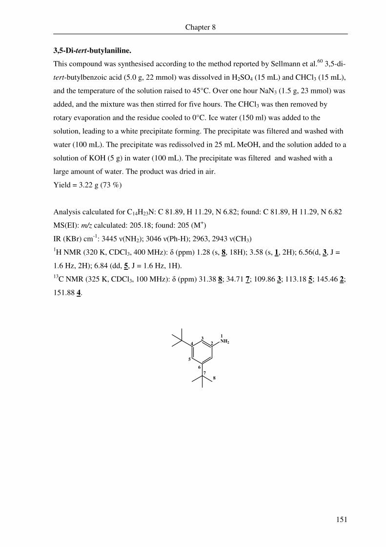
Chapter 8
151
3,5-Di-tert-butylaniline.
This compound was synthesised according to the method reported by Sellmann et al.60 3,5-di-
tert-butylbenzoic acid (5.0 g, 22 mmol) was dissolved in H2SO4 (15 mL) and CHCl3 (15 mL),
and the temperature of the solution raised to 45°C. Over one hour NaN3 (1.5 g, 23 mmol) was
added, and the mixture was then stirred for five hours. The CHCl3 was then removed by
rotary evaporation and the residue cooled to 0°C. Ice water (150 ml) was added to the
solution, leading to a white precipitate forming. The precipitate was filtered and washed with
water (100 mL). The precipitate was redissolved in 25 mL MeOH, and the solution added to a
solution of KOH (5 g) in water (100 mL). The precipitate was filtered and washed with a
large amount of water. The product was dried in air.
Yield = 3.22 g (73 %)
Analysis calculated for C14H23N: C 81.89, H 11.29, N 6.82; found: C 81.89, H 11.29, N 6.82
MS(EI): m/z calculated: 205.18; found: 205 (M+)
IR (KBr) cm-1: 3445 ν(NH2); 3046 ν(Ph-H); 2963, 2943 ν(CH3) 1H NMR (320 K, CDCl3, 400 MHz): δ (ppm) 1.28 (s, 8, 18H); 3.58 (s, 1, 2H); 6.56(d, 3, J =
1.6 Hz, 2H); 6.84 (dd, 5, J = 1.6 Hz, 1H). 13C NMR (325 K, CDCl3, 100 MHz): δ (ppm) 31.38 8; 34.71 7; 109.86 3; 113.18 5; 145.46 2;
151.88 4.
1
23
4
5
6
78
NH2
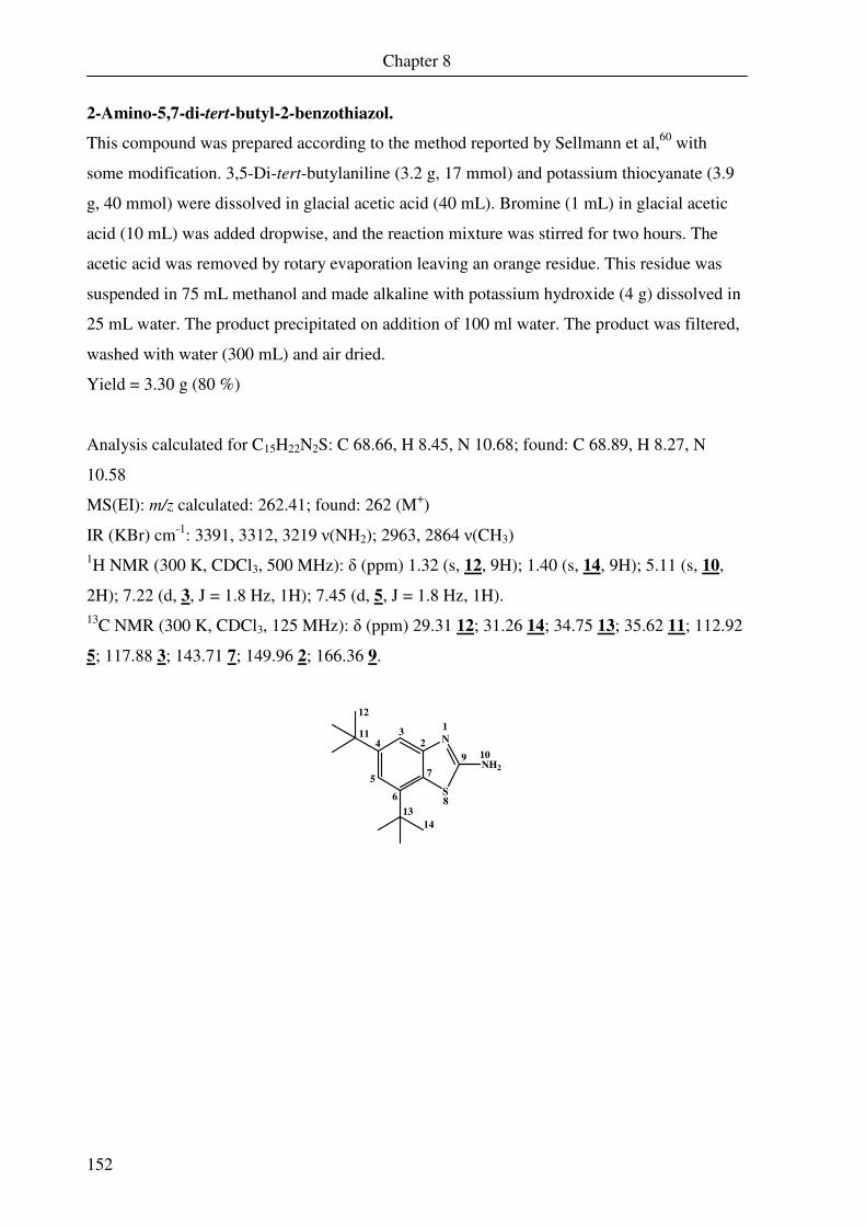
Chapter 8
152
2-Amino-5,7-di-tert-butyl-2-benzothiazol.
This compound was prepared according to the method reported by Sellmann et al,60 with
some modification. 3,5-Di-tert-butylaniline (3.2 g, 17 mmol) and potassium thiocyanate (3.9
g, 40 mmol) were dissolved in glacial acetic acid (40 mL). Bromine (1 mL) in glacial acetic
acid (10 mL) was added dropwise, and the reaction mixture was stirred for two hours. The
acetic acid was removed by rotary evaporation leaving an orange residue. This residue was
suspended in 75 mL methanol and made alkaline with potassium hydroxide (4 g) dissolved in
25 mL water. The product precipitated on addition of 100 ml water. The product was filtered,
washed with water (300 mL) and air dried.
Yield = 3.30 g (80 %)
Analysis calculated for C15H22N2S: C 68.66, H 8.45, N 10.68; found: C 68.89, H 8.27, N
10.58
MS(EI): m/z calculated: 262.41; found: 262 (M+)
IR (KBr) cm-1: 3391, 3312, 3219 ν(NH2); 2963, 2864 ν(CH3) 1H NMR (300 K, CDCl3, 500 MHz): δ (ppm) 1.32 (s, 12, 9H); 1.40 (s, 14, 9H); 5.11 (s, 10,
2H); 7.22 (d, 3, J = 1.8 Hz, 1H); 7.45 (d, 5, J = 1.8 Hz, 1H). 13C NMR (300 K, CDCl3, 125 MHz): δ (ppm) 29.31 12; 31.26 14; 34.75 13; 35.62 11; 112.92
5; 117.88 3; 143.71 7; 149.96 2; 166.36 9.
1
23
4
5
6
7
8
9 10
11
12
N
S
NH2
13
14

Chapter 8
153
2-Mercapto-3,5-di-tert-butylaniline.
This procedure was adapted from a report published by Sellmann et al.60 2-Amino-5,7-di-tert-
butyl-2-benzothiazol (3.30 g, 13 mmol) and potassium hydroxide (30 g, 0.53 mol) were
suspended in 2,3-butadiol (40 mL). This mixture was refluxed under argon for three hours at
200°C. The reaction mixture was then allowed to cool to less than 100°C. Acetic acid (50 mL)
and water (200 mL) were added to the warm solution. The product was extracted into diethyl
ether (150 mL), washed with water (2 × 100 mL) and dried over Na2SO4. The solvent is
removed on vacuum line, leaving a viscous yellow green oil. The product is used immediately
without further purification due to extreme sensitivity to air. The oil also contains some
residual 2,3-butadiol, as seen in the proton NMR.
Yield = 2.9 g (72 %)
MS(EI): m/z calculated: 237.4; found: 237 (M+)
IR (KBr) cm-1: 3476 ν(NH2); 2925, 2962 ν(CH3) 1H NMR (300 K, CDCl3, 400 MHz): δ (ppm) 1.26 (s, 12, 9H); 1.51 (s, 10, 9H), 3.51 (s, 1,
2H); 3.78 (s, 8, 1H); 6.71 (s, 3, 1H); 6.92 (s, 5, 1H).
NH2
SH
1
23
4
5
6
7
89
10
11
12
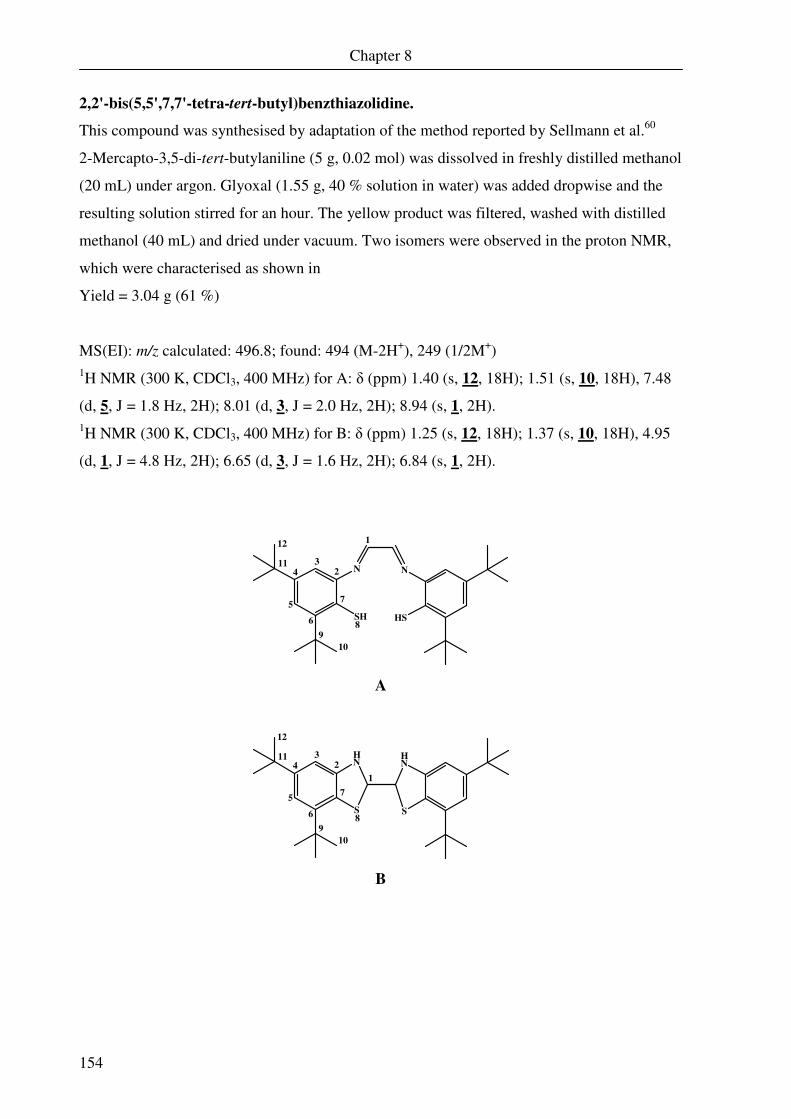
Chapter 8
154
2,2'-bis(5,5',7,7'-tetra-tert-butyl)benzthiazolidine.
This compound was synthesised by adaptation of the method reported by Sellmann et al.60
2-Mercapto-3,5-di-tert-butylaniline (5 g, 0.02 mol) was dissolved in freshly distilled methanol
(20 mL) under argon. Glyoxal (1.55 g, 40 % solution in water) was added dropwise and the
resulting solution stirred for an hour. The yellow product was filtered, washed with distilled
methanol (40 mL) and dried under vacuum. Two isomers were observed in the proton NMR,
which were characterised as shown in
Yield = 3.04 g (61 %)
MS(EI): m/z calculated: 496.8; found: 494 (M-2H+), 249 (1/2M+) 1H NMR (300 K, CDCl3, 400 MHz) for A: δ (ppm) 1.40 (s, 12, 18H); 1.51 (s, 10, 18H), 7.48
(d, 5, J = 1.8 Hz, 2H); 8.01 (d, 3, J = 2.0 Hz, 2H); 8.94 (s, 1, 2H). 1H NMR (300 K, CDCl3, 400 MHz) for B: δ (ppm) 1.25 (s, 12, 18H); 1.37 (s, 10, 18H), 4.95
(d, 1, J = 4.8 Hz, 2H); 6.65 (d, 3, J = 1.6 Hz, 2H); 6.84 (s, 1, 2H).
N
SH
1
23
4
5
6
7
89
10
11
12
N
HS
A
HN
S
1
23
4
5
6
7
89
10
11
12
HN
S
B
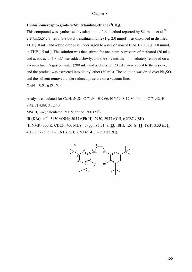
Chapter 8
155
1,2-bis(2-mercapto-3,5-di-tert-butylaniline)ethane (2LH4).
This compound was synthesised by adaptation of the method reported by Sellmann et al.60
2,2'-bis(5,5',7,7'-tetra-tert-butyl)benzthiazolidine (1 g, 2.0 mmol) was dissolved in distilled
THF (10 mL) and added dropwise under argon to a suspension of LiAlH4 (0.32 g, 7.8 mmol)
in THF (15 mL). The solution was then stirred for one hour. A mixture of methanol (20 mL)
and acetic acid (10 mL) was added slowly, and the solvents then immediately removed on a
vacuum line. Degassed water (200 mL) and acetic acid (20 mL) were added to the residue,
and the product was extracted into diethyl ether (80 mL). The solution was dried over Na2SO4
and the solvent removed under reduced pressure on a vacuum line.
Yield = 0.91 g (91 %)
Analysis calculated for C30H48N2S2: C 71.94, H 9.66, N 5.59, S 12.80; found: C 71.42, H
9.42, N 4.89, S 12.40.
MS(EI): m/z calculated: 500.9; found: 500 (M+)
IR (KBr) cm-1: 3430 ν(NH); 3055 ν(Ph-H); 2930, 2955 ν(CH3); 2587 ν(SH) 1H NMR (300 K, CDCl3, 400 MHz): δ (ppm) 1.31 (s, 13, 18H); 1.51 (s, 11, 18H), 3.53 (s, 1,
4H); 6.67 (d, 6, J = 1.6 Hz, 2H); 6.93 (d, 4, J = 2.0 Hz 2H).
NH
SH
1
2
34
5
6
7
8
9
10
11
12HN
HS
13

Chapter 8
156
1,3-bis[benzthiazolonyl(3)]propane.
A solution of 2-hydroxybenzothiazole (3.95 g, 0.026 mol) in ethanol (30 mL) was heated to
reflux and 1,3-dibromopropane (2.64 g, 0.013 mol) was added dropwise. The mixture was
heated to reflux for seven hours. The solution was cooled to room temperature, the cream
coloured precipitate filtered off and washed repeatedly with cold ethanol.
Yield = 2.95 g (66 %)
Analysis calculated for C17H14N2O 2S2: C 59.63, H 4.12, N 8.18, S 18.73; found: C 59.68, H
4.18, N 8.10, S 18.68.
MS(EI): m/z calculated: 342.44; found: 342 (M+)
IR (KBr) cm-1: 2923, 2864 ν(CH3); 1625 ν(C=O) 1H NMR (300 K, CDCl3, 500 MHz): δ (ppm) 1.32 (s, 12, 9H); 1.40 (s, 14, 9H); 2.09 (s, 10,
2H); 7.22 (d, 3, J = 1.8 Hz, 1H); 7.45 (d, 5, J = 1.8 Hz, 1H). 13C NMR (300 K, CDCl3, 100 MHz): δ (ppm) 29.54 1;
S
N N
S
O O
1
2
34
5
6
78
9
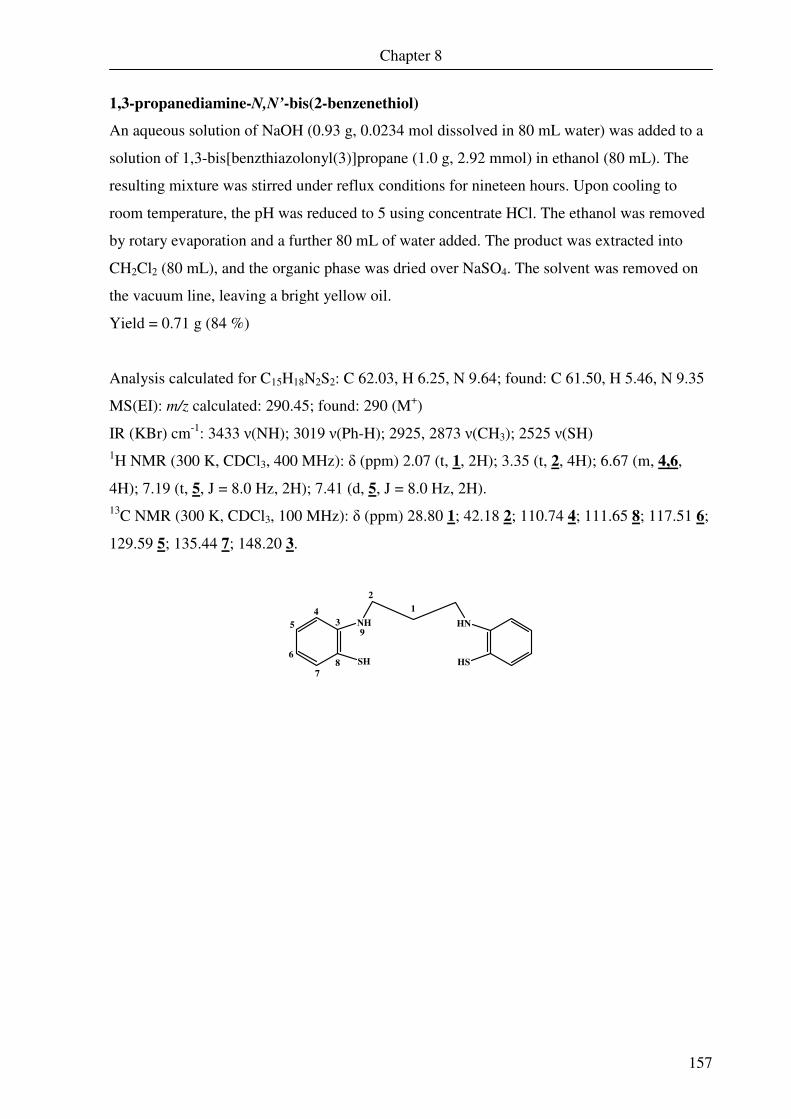
Chapter 8
157
1,3-propanediamine-N,N’-bis(2-benzenethiol)
An aqueous solution of NaOH (0.93 g, 0.0234 mol dissolved in 80 mL water) was added to a
solution of 1,3-bis[benzthiazolonyl(3)]propane (1.0 g, 2.92 mmol) in ethanol (80 mL). The
resulting mixture was stirred under reflux conditions for nineteen hours. Upon cooling to
room temperature, the pH was reduced to 5 using concentrate HCl. The ethanol was removed
by rotary evaporation and a further 80 mL of water added. The product was extracted into
CH2Cl2 (80 mL), and the organic phase was dried over NaSO4. The solvent was removed on
the vacuum line, leaving a bright yellow oil.
Yield = 0.71 g (84 %)
Analysis calculated for C15H18N2S2: C 62.03, H 6.25, N 9.64; found: C 61.50, H 5.46, N 9.35
MS(EI): m/z calculated: 290.45; found: 290 (M+)
IR (KBr) cm-1: 3433 ν(NH); 3019 ν(Ph-H); 2925, 2873 ν(CH3); 2525 ν(SH) 1H NMR (300 K, CDCl3, 400 MHz): δ (ppm) 2.07 (t, 1, 2H); 3.35 (t, 2, 4H); 6.67 (m, 4,6,
4H); 7.19 (t, 5, J = 8.0 Hz, 2H); 7.41 (d, 5, J = 8.0 Hz, 2H). 13C NMR (300 K, CDCl3, 100 MHz): δ (ppm) 28.80 1; 42.18 2; 110.74 4; 111.65 8; 117.51 6;
129.59 5; 135.44 7; 148.20 3.
SH
NH HN
HS
1
2
34
5
6
78
9
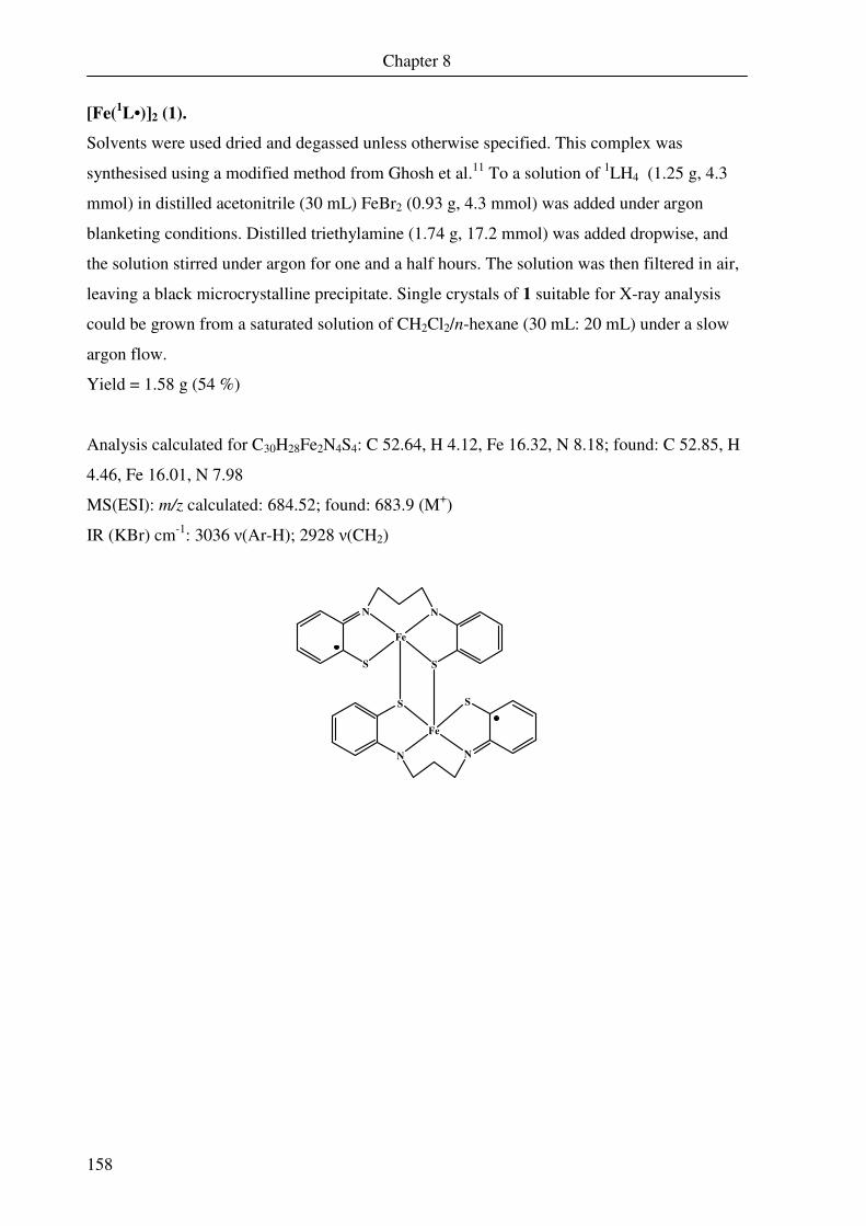
Chapter 8
158
[Fe(1L•)]2 (1).
Solvents were used dried and degassed unless otherwise specified. This complex was
synthesised using a modified method from Ghosh et al.11 To a solution of 1LH4 (1.25 g, 4.3
mmol) in distilled acetonitrile (30 mL) FeBr2 (0.93 g, 4.3 mmol) was added under argon
blanketing conditions. Distilled triethylamine (1.74 g, 17.2 mmol) was added dropwise, and
the solution stirred under argon for one and a half hours. The solution was then filtered in air,
leaving a black microcrystalline precipitate. Single crystals of 1 suitable for X-ray analysis
could be grown from a saturated solution of CH2Cl2/n-hexane (30 mL: 20 mL) under a slow
argon flow.
Yield = 1.58 g (54 %)
Analysis calculated for C30H28Fe2N4S4: C 52.64, H 4.12, Fe 16.32, N 8.18; found: C 52.85, H
4.46, Fe 16.01, N 7.98
MS(ESI): m/z calculated: 684.52; found: 683.9 (M+)
IR (KBr) cm-1: 3036 ν(Ar-H); 2928 ν(CH2)
N
S
N
S
Fe
N
S
N
S
Fe
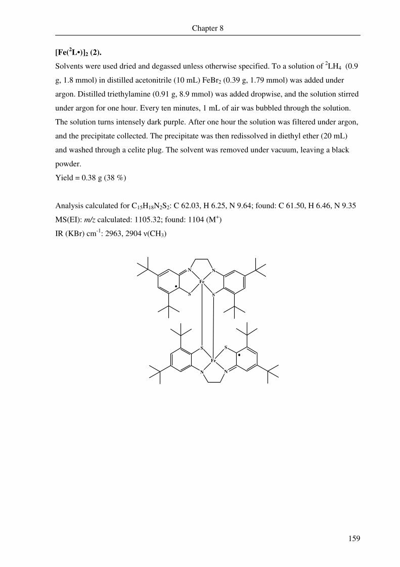
Chapter 8
159
[Fe(2L•)]2 (2).
Solvents were used dried and degassed unless otherwise specified. To a solution of 2LH4 (0.9
g, 1.8 mmol) in distilled acetonitrile (10 mL) FeBr2 (0.39 g, 1.79 mmol) was added under
argon. Distilled triethylamine (0.91 g, 8.9 mmol) was added dropwise, and the solution stirred
under argon for one hour. Every ten minutes, 1 mL of air was bubbled through the solution.
The solution turns intensely dark purple. After one hour the solution was filtered under argon,
and the precipitate collected. The precipitate was then redissolved in diethyl ether (20 mL)
and washed through a celite plug. The solvent was removed under vacuum, leaving a black
powder.
Yield = 0.38 g (38 %)
Analysis calculated for C15H18N2S2: C 62.03, H 6.25, N 9.64; found: C 61.50, H 6.46, N 9.35
MS(EI): m/z calculated: 1105.32; found: 1104 (M+)
IR (KBr) cm-1: 2963, 2904 ν(CH3)
N
S
N
S
Fe
N
S
N
S
Fe
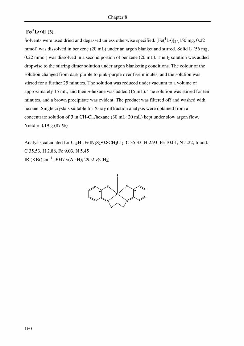
Chapter 8
160
[Fe(1L••)I] (3).
Solvents were used dried and degassed unless otherwise specified. [Fe(1L•)]2 (150 mg, 0.22
mmol) was dissolved in benzene (20 mL) under an argon blanket and stirred. Solid I2 (56 mg,
0.22 mmol) was dissolved in a second portion of benzene (20 mL). The I2 solution was added
dropwise to the stirring dimer solution under argon blanketing conditions. The colour of the
solution changed from dark purple to pink-purple over five minutes, and the solution was
stirred for a further 25 minutes. The solution was reduced under vacuum to a volume of
approximately 15 mL, and then n-hexane was added (15 mL). The solution was stirred for ten
minutes, and a brown precipitate was evident. The product was filtered off and washed with
hexane. Single crystals suitable for X-ray diffraction analysis were obtained from a
concentrate solution of 3 in CH2Cl2/hexane (30 mL: 20 mL) kept under slow argon flow.
Yield = 0.19 g (87 %)
Analysis calculated for C15H14FeIN2S2•0.8CH2Cl2: C 35.33, H 2.93, Fe 10.01, N 5.22; found:
C 35.53, H 2.88, Fe 9.03, N 5.45
IR (KBr) cm-1: 3047 ν(Ar-H); 2952 ν(CH2)
I
N
S
N
S
Fe
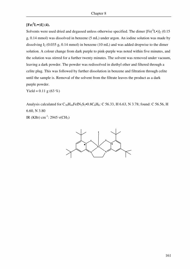
Chapter 8
161
[Fe(2L••)I] (4).
Solvents were used dried and degassed unless otherwise specified. The dimer [Fe(2L•)]2 (0.15
g, 0.14 mmol) was dissolved in benzene (5 mL) under argon. An iodine solution was made by
dissolving I2 (0.035 g, 0.14 mmol) in benzene (10 mL) and was added dropwise to the dimer
solution. A colour change from dark purple to pink-purple was noted within five minutes, and
the solution was stirred for a further twenty minutes. The solvent was removed under vacuum,
leaving a dark powder. The powder was redissolved in diethyl ether and filtered through a
celite plug. This was followed by further dissolution in benzene and filtration through celite
until the sample is. Removal of the solvent from the filtrate leaves the product as a dark
purple powder.
Yield = 0.11 g (63 %)
Analysis calculated for C30H44FeIN2S2•0.8C6H6: C 56.33, H 6.63, N 3.78; found: C 56.56, H
6.60, N 3.80
IR (KBr) cm-1: 2945 ν(CH3)
I
N
S
N
S
Fe

Chapter 8
162
[Fe(1L••)(P(CH3)3)] (5).
Complex 1 (0.20 g, 0.29 mmol) was suspended in dry benzene (10 mL) under an argon
blanket, and a solution of P(CH3)3 in toluene (1 M, 0.584 mL) was added slowly. The solution
immediately changed from dark purple to dark green. The solution was stirred for a further
ten minutes, then dry hexane was added (30 mL). After stirring for ten minutes a green
microcrystalline solid was apparent. The solution was filtered, leaving the green compound 5.
Single crystals suitable for X-ray analysis were grown from the slow evaporation of a
concentrate solution of 5 in dichloromethane:hexane (3:2).
Yield = 0.14 g (58 %)
Analysis calculated for C18H23FePN2S2: C 51.68, H 5.54, Fe 13.35, N 6.70, S 15.53; found: C
51.46, H 5.60, Fe 13.22, N 6.55, S 15.41
IR (KBr) cm-1: 3045 ν(Ar-H); 2963 ν(CH2); 941 ν(PCH3)
P
N
S
N
S
Fe
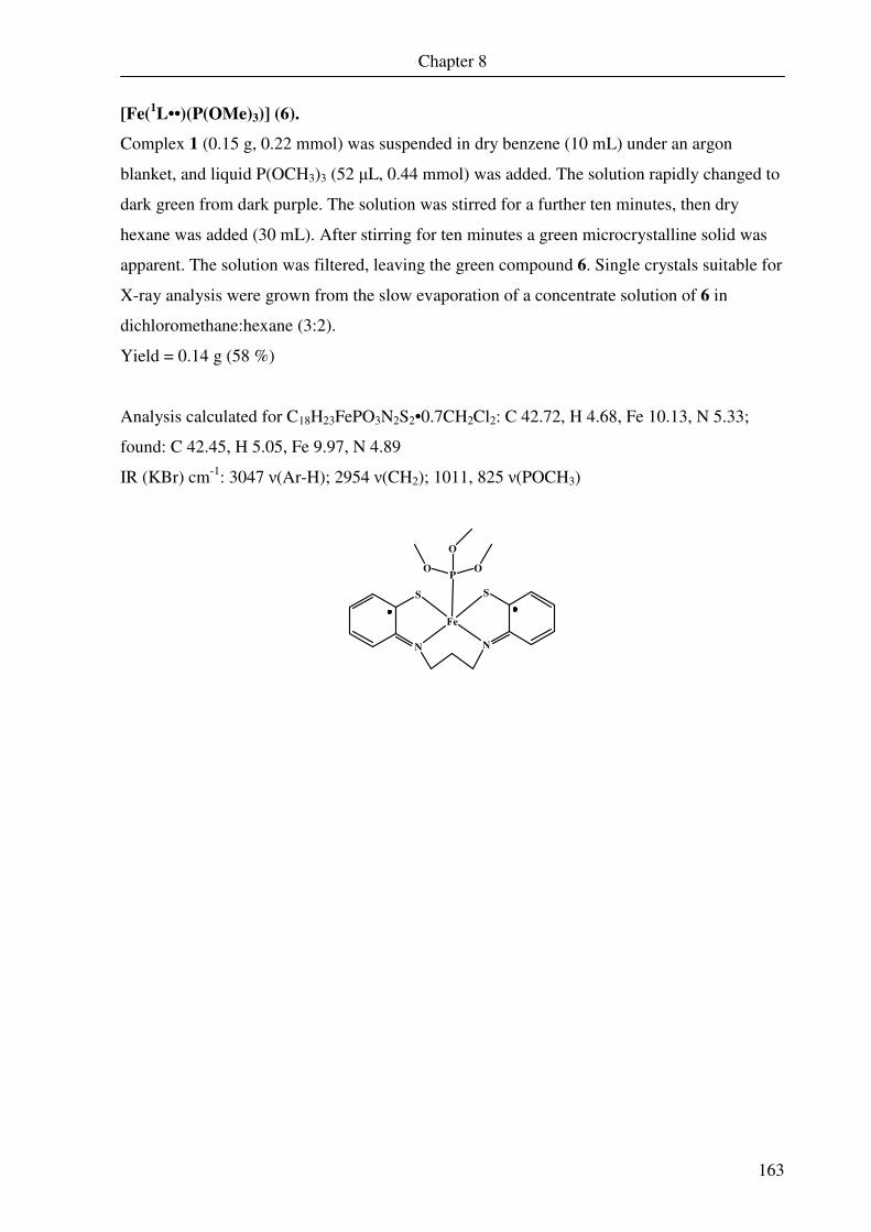
Chapter 8
163
[Fe(1L••)(P(OMe)3)] (6).
Complex 1 (0.15 g, 0.22 mmol) was suspended in dry benzene (10 mL) under an argon
blanket, and liquid P(OCH3)3 (52 µL, 0.44 mmol) was added. The solution rapidly changed to
dark green from dark purple. The solution was stirred for a further ten minutes, then dry
hexane was added (30 mL). After stirring for ten minutes a green microcrystalline solid was
apparent. The solution was filtered, leaving the green compound 6. Single crystals suitable for
X-ray analysis were grown from the slow evaporation of a concentrate solution of 6 in
dichloromethane:hexane (3:2).
Yield = 0.14 g (58 %)
Analysis calculated for C18H23FePO3N2S2•0.7CH2Cl2: C 42.72, H 4.68, Fe 10.13, N 5.33;
found: C 42.45, H 5.05, Fe 9.97, N 4.89
IR (KBr) cm-1: 3047 ν(Ar-H); 2954 ν(CH2); 1011, 825 ν(POCH3)
P
N
S
N
S
Fe
O
O
O
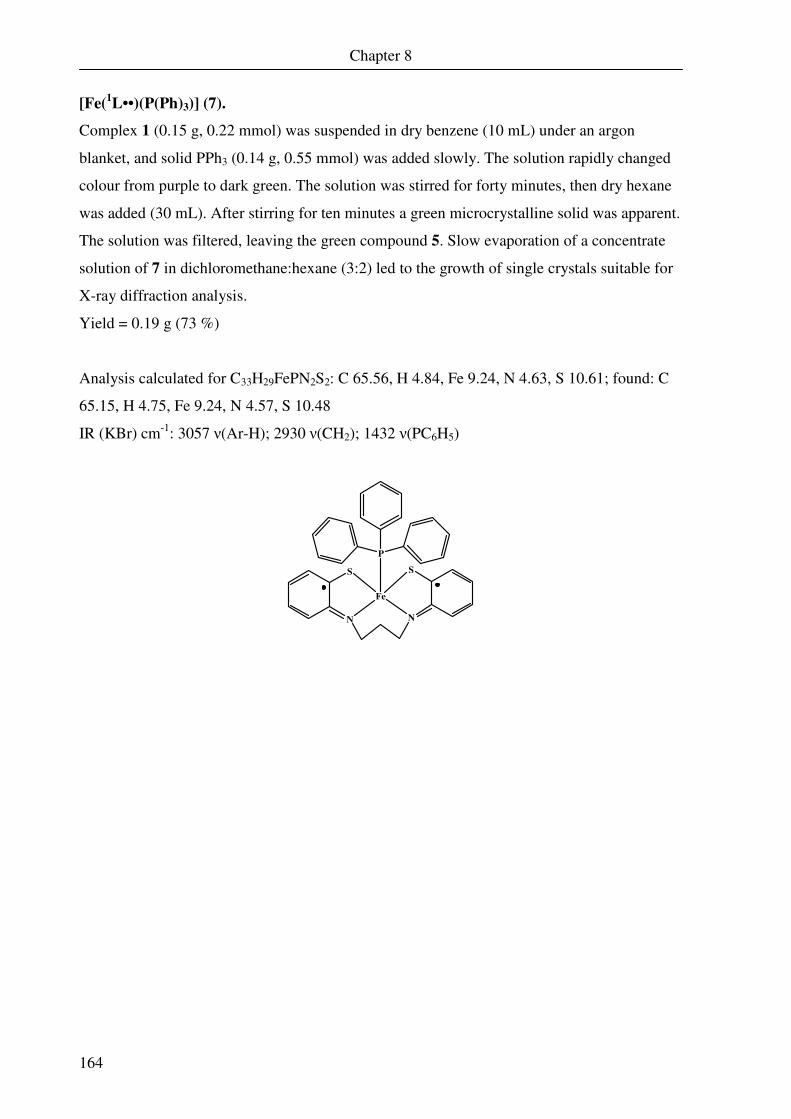
Chapter 8
164
[Fe(1L••)(P(Ph)3)] (7).
Complex 1 (0.15 g, 0.22 mmol) was suspended in dry benzene (10 mL) under an argon
blanket, and solid PPh3 (0.14 g, 0.55 mmol) was added slowly. The solution rapidly changed
colour from purple to dark green. The solution was stirred for forty minutes, then dry hexane
was added (30 mL). After stirring for ten minutes a green microcrystalline solid was apparent.
The solution was filtered, leaving the green compound 5. Slow evaporation of a concentrate
solution of 7 in dichloromethane:hexane (3:2) led to the growth of single crystals suitable for
X-ray diffraction analysis.
Yield = 0.19 g (73 %)
Analysis calculated for C33H29FePN2S2: C 65.56, H 4.84, Fe 9.24, N 4.63, S 10.61; found: C
65.15, H 4.75, Fe 9.24, N 4.57, S 10.48
IR (KBr) cm-1: 3057 ν(Ar-H); 2930 ν(CH2); 1432 ν(PC6H5)
P
N
S
N
S
Fe

Chapter 8
165
[Fe(1L••)(P(OPh)3)] (8).
Complex 1 (0.15 g, 0.22 mmol) was suspended in dry toluene (10 mL) under an argon
blanket, and liquid P(OPh)3 (0.17 g, 0.55 mmol) was added slowly. The solution rapidly
changed colour from purple to dark green. The solution was stirred under argon for forty
minutes, then dry hexane was added (30 mL). After stirring for ten minutes a dark precipitate
forms. The solution was filtered, leaving the dark green compound 8. Single crystals suitable
for X-ray diffraction analysis were grown from slow evaporation of a concentrate solution of
8 in dichloromethane:hexane (2:1, 200 mL).
Yield = 0.20 g (70 %)
Analysis calculated for C33H29FePO3N2S2•0.15CH2Cl2: C 59.85, H 4.44, Fe 8.39, N 4.21;
found: C 59.96, H 4.61, Fe 7.48, N 4.35
IR (KBr) cm-1: 3069 ν(Ar-H); 2928 ν(CH2); 1187, 922 ν(POC6H5)
P
N
S
N
S
Fe
O
O
O
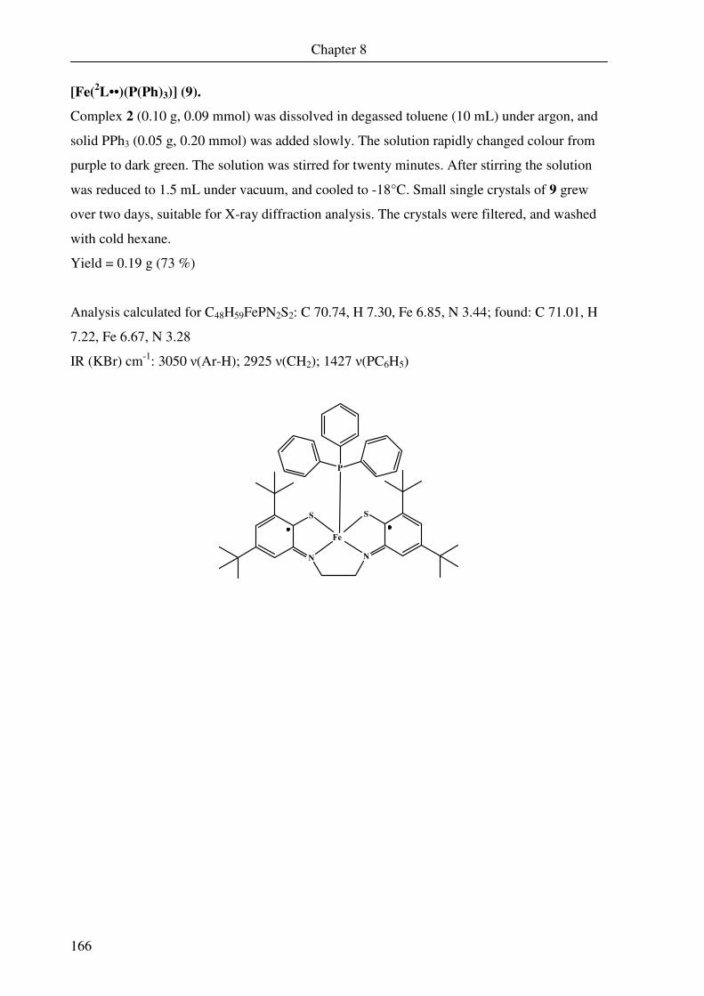
Chapter 8
166
[Fe(2L••)(P(Ph)3)] (9).
Complex 2 (0.10 g, 0.09 mmol) was dissolved in degassed toluene (10 mL) under argon, and
solid PPh3 (0.05 g, 0.20 mmol) was added slowly. The solution rapidly changed colour from
purple to dark green. The solution was stirred for twenty minutes. After stirring the solution
was reduced to 1.5 mL under vacuum, and cooled to -18°C. Small single crystals of 9 grew
over two days, suitable for X-ray diffraction analysis. The crystals were filtered, and washed
with cold hexane.
Yield = 0.19 g (73 %)
Analysis calculated for C48H59FePN2S2: C 70.74, H 7.30, Fe 6.85, N 3.44; found: C 71.01, H
7.22, Fe 6.67, N 3.28
IR (KBr) cm-1: 3050 ν(Ar-H); 2925 ν(CH2); 1427 ν(PC6H5)
N
S
N
S
FeI
P
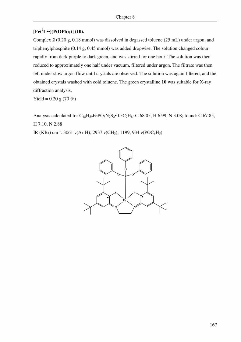
Chapter 8
167
[Fe(2L••)(P(OPh)3)] (10).
Complex 2 (0.20 g, 0.18 mmol) was dissolved in degassed toluene (25 mL) under argon, and
triphenylphosphite (0.14 g, 0.45 mmol) was added dropwise. The solution changed colour
rapidly from dark purple to dark green, and was stirred for one hour. The solution was then
reduced to approximately one half under vacuum, filtered under argon. The filtrate was then
left under slow argon flow until crystals are observed. The solution was again filtered, and the
obtained crystals washed with cold toluene. The green crystalline 10 was suitable for X-ray
diffraction analysis.
Yield = 0.20 g (70 %)
Analysis calculated for C48H59FePO3N2S2•0.5C7H8: C 68.05, H 6.99, N 3.08; found: C 67.85,
H 7.10, N 2.88
IR (KBr) cm-1: 3061 ν(Ar-H); 2937 ν(CH3); 1199, 934 ν(POC6H5)
N
S
N
S
FeI
P
O
OO

Chapter 8
168
[Fe(2Lgma•)(
t-Bupy)] (11).
Complex 2 (0.10 g, 0.09 mmol) was dissolved in degassed toluene (5 mL) and 4-tert-
butylpyridine (0.12 g, 0.91 mmol) was added dropwise. The solution was stirred for thirty
minutes followed by bubbling of twenty mL of air. The purple solution was left to evaporate
under argon flow, and the colour changed over a period of days from purple to reddish-brown.
Continual evaporation led to formation of black crystals of 11, which were filtered off and
washed with cold hexane. These crystals proved sufficient for X-ray diffraction analysis.
Yield = 0.06 g (40 %)
Analysis calculated for C39H57FeN3S2•2C10H13N: C 71.59, H 8.54, Fe 5.84, N 7.32, S 6.71;
found: C 71.48, H 8.43, Fe 5.88, N 7.34, S 6.80
IR (KBr) cm-1: 3025 ν(Ar-H); 2947 ν(CH3); 1605 ν(C=N)py; 1562 ν(C=N)
N
S
N
S
FeI
N

169
CHAPTER 9
Bibliography

170
Chapter 9
171
(1) Sumner, J. B. J. Biol. Chem. 1919, xxxviii, 59.
(2) Benini, S.; Rypniewski, W. R.; Wilson, K. S.; Miletti, S.; Ciurli, S.; Mangani, S. Structure 1999, 7, 205.
(3) Dixon, N. E.; Gazzola, T. C.; Blakeley, R. L.; Zermer, B. J. Am. Chem. Soc.
1975, 97, 4131. (4) Baron, A. J.; Stevens, C.; Wilmot, C.; Seneviratnes, K. D.; Blakeley, V.;
Dooley, D. M.; Phillips, S. E. V.; Knowles, P. F.; McPherson, M. J. J. Biol.
Chem. 1994, 269, 25095. (5) Metalloenzymes Involving Amino Acid-Residues and Related Radicals; Sigel,
H.; Sigel, A., Eds.; Marcel Decker: New York, 1994; Vol. 30. (6) Hegedus, L. S. Transition Metals in the Synthesis of Complex Organic
Molecules; University Science Books: Mill Valley, CA, 1994. (7) Jørgenson, C. K. Oxidation Numbers and Oxidation States; Springer:
Heidelberg, Germany, 1969. (8) Sellmann, D.; Emig, S.; Heinemann, F. W.; Knoch, F. Angew. Chem., Int. Ed.
Engl. 1997, 36, 1201-1203. (9) Sellmann, D.; Geck, M.; Knoch, F.; Ritter, G.; Dengler, J. J. Am. Chem. Soc.
1991, 113, 3819-28. (10) Sellmann, D.; Emig, S.; Heinemann, F. Angew. Chem., Int. Ed. Engl. 1997, 36,
1734-1736. (11) Ghosh, P.; Bill, E.; Weyhermüller, T.; Wieghardt, K. J. Am. Chem. Soc. 2003,
125, 3967-3979. (12) Szilagyi, R. K.; Lim, B. S.; Glaser, T.; Holm, R. H.; Hedman, B.; Hodgson, K.
O.; Solomon, E. I. J. Am. Chem. Soc. 2003, 125, 9158.
(13) Schrauzer, G. N.; Mayweg, V. J. Am. Chem. Soc. 1962, 84, 3221.
(14) Gray, H. B.; Williams, R.; Bernal, I.; Billig, E. J. Am. Chem. Soc. 1962, 84, 3596.
(15) Davison, A.; Edelstein, N.; Holm, R. H.; Maki, A. H. Inorg. Chem. 1963, 2,
1227. (16) Davison, A.; Edelstein, N.; Holm, R. H.; Maki, A. H. J. Am. Chem. Soc. 1963,
85, 2029.
(17) Baker-Hawkes, M. J.; Billig, E.; Gray, H. B. J. Am. Chem. Soc. 1966, 88, 4870. (18) Balch, A. L.; Holm, R. H. Chem. Commun. 1966, 15, 552.
Chapter 9
172
(19) Enemark, J. H.; Lipscomb, W. N. Inorg. Chem. 1965, 4, 1729. (20) Hamilton, W. C.; Bernal, I. Inorg. Chem. 1967, 6, 2003. (21) Birchall, T.; Greenwodd, N. N. J. Chem. Soc. (A) 1969, 286.
(22) Sellmann, D.; Binder, H.; Haussinger, D.; Heinemann, F. W.; Sutter, J. Inorg.
Chim. Acta 2000, 300-302, 829-836.
(23) Beloglazkina, E. K.; Moiseeva, A. A.; Chizhevskii, A. A.; Tarasevich, B. N.; Zyk, N. V.; Butin, K. P. Russ. Chem. Bull. Int. Ed. 2003, 52, 1990.
(24) Ghosh, P.; Stobie, K.; Bill, E.; Bothe, E.; Weyhermüller, T.; Ward, M. D.;
McCleverty, J. A.; Wieghardt, K. Inorg. Chem. 2007, 46, 522-532.
(25) Patra, A. K.; Bill, E.; Bothe, E.; Chlopek, K.; Neese, F.; Weyhermüller, T.; Stobie, K.; Ward, M. D.; McCleverty, J. A.; Wieghardt, K. Inorg. Chem. 2006, 45, 7877-7890.
(26) Ray, K.; Begum, A.; Weyhermüller, T.; Piligkos, S.; Van Slageren, J.; Neese,
F.; Wieghardt, K. J. Am. Chem. Soc. 2005, 127, 4403-4415.
(27) Ray, K.; Bill, E.; Weyhermüller, T.; Wieghardt, K. J. Am. Chem. Soc. 2005, 127, 5641-5654.
(28) Ray, K.; George, S. D.; Solomon, E. I.; Wieghardt, K.; Neese, F. Chem. Eur. J.
2007, 13, 2783-2797. (29) Ray, K.; Weyhermüller, T.; Goossens, A.; Craje, M. W. J.; Wieghardt, K.
Inorg. Chem. 2003, 42, 4082-4087. (30) Ray, K.; Weyhermüller, T.; Neese, F.; Wieghardt, K. Inorg. Chem. 2005, 44,
5345-5360.
(31) Balch, A. L.; Holm, R. H. J. Am. Chem. Soc. 1966, 88, 5201.
(32) Stiefel, E. I.; Waters, J. H.; Billig, E.; Gray, H. B. J. Am. Chem. Soc. 1965, 87, 3016.
(33) Christoph, G. C.; Goedken, V. L. J. Am. Chem. Soc. 1973, 95, 3869.
(34) Gerber, T. I. A.; Kemp, H. J.; du Preez, J. G. H.; Bandoli, G.; Dolmella, A. Inorg. Chim. Acta 1992, 202.
(35) Peng, S.-M.; Chen, C.-T.; Liaw, D.-S.; Chen, C.-I.; Wang, Y. Inorg. Chim.
Acta 1985, 101, L31. (36) Herebian, D.; Bothe, E.; Neese, F.; Weyhermüller, T.; Wieghardt, K. J. Am.
Chem. Soc. 2003, 125, 9116-9128.
Chapter 9
173
(37) Chlopek, K.; Bill, E.; Weyhermüller, T.; Wieghardt, K. Inorg. Chem. 2005, 44, 7087-7098.
(38) Chlopek, K., Ruhr-Universität, 2005. (39) Larkworthy, L. F.; Murphy, J. M.; Phillips, D. J. Inorg. Chem. 1968, 7, 1436. (40) Le Borgne, G.; Grandjean, D. Acta Crystallogr. 1973, B29, 1040.
(41) Ghosh, P.; Begum, A.; Bill, E.; Weyhermüller, T.; Wieghardt, K. Inorg. Chem. 2003, 42, 3208.
(42) Kawamoto, T.; Kuma, H.; Kushi, Y. Bull. Chem. Soc. Jpn. 1997, 70, 1599.
(43) Chlopek, K.; Muresan, N.; Neese, F.; Wieghardt, K. Chem. Eur. J. 2007, 13, 8390-8403.
(44) Ghosh, P.; Begum, A.; Bill, E.; Weyhermüller, T.; Wieghardt, K. Inorg. Chem.
2003, 42, 3208-3215. (45) Gardiner, M. G.; Hanson, G. R.; Henderson, M. J.; Lee, F. C.; Raston, C. L.
Inorg. Chem. 1994, 33, 2456. (46) Bart, S. C.; Hawrelak, E. J.; Lobkovsky, E.; Chirik, P. Organometallics 2005,
24, 5518.
(47) tom Dieck, H.; Bruder, H. J. Chem. Soc., Chem. Comm. 1977, 24, 149. (48) Walther, D.; Kreisel, G.; Kirmse, R. Z. Anorg. Allg. Chem. 1982, 487.
(49) Blanchard, S.; Neese, F.; Bothe, E.; Bill, E.; Weyhermüller, T.; Wieghardt, K. Inorg. Chem. 2005, 44, 3636-3656.
(50) Chlopek, K.; Bothe, E.; Neese, F.; Weyhermüller, T.; Wieghardt, K. Inorg.
Chem. 2006, 45, 6298-6307. (51) Khusniyarov, M. M.; Harms, K.; Burghaus, O.; Sundermeyer, J. Eur. J. Inorg.
Chem. 2006, 15, 2985. (52) Muresan, N.; Chlopek, K.; Weyhermüller, T.; Neese, F.; Wieghardt, K. Inorg.
Chem. 2007, 46, 5327-5337. (53) Spikes, G. H.; Bill, E.; Weyhermüller, T.; Wieghardt, K. Angew. Chem. Int.
Ed. 2008, 47, 2973. (54) Muresan, N.; Chlopek, K.; Weyhermüller, T.; Neese, F.; Wieghardt, K. Inorg.
Chem. 2007, 46, 5327-5337. (55) Spikes, G. H.; Bill, E.; Weyhermüller, T.; Wieghardt, K. Chem. Commun.
2007, 4339-4341.
Chapter 9
174
(56) Sellmann, D.; Hannakam, M.; Knoch, F.; Moll, M. Z. Naturforsch. 1992, 47b, 1545.
(57) Karsten, P.; Maichle-Mössmer, C.; Strähle, J. Z. Anorg. Allg. Chem. 1997, 623,
1644. (58) Ghosh, P.; Bill, E.; Weyhermüller, T.; Neese, F.; Wieghardt, K. J. Am. Chem.
Soc. 2003, 125, 1293.
(59) Sellmann, D.; Ruf, R.; Knoch, F.; Moll, M. Inorg. Chem. 1995, 34, 4745.
(60) Sellmann, D.; Emig, S.; Heinemann, F. W.; Knoch, F. Z. Naturforsch., B:
Chem. Sci. 1998, 53, 1461-1474.
(61) Balch, A. L.; Dance, I. G.; Holm, R. H. J. Am. Chem. Soc. 1968, 90, 1139.
(62) Sawyer, D. T.; Srivatsa, G. S.; Bodini, M. E.; Schaefer, W. P.; Wing, R. M. J.
Am. Chem. Soc. 1986, 108, 936. (63) Kang, B. S.; Weng, L. H.; Wu, D. X.; Wang, F.; Guo, Z.; Huang, L. R.; Huang,
Z. Y.; Liu, H. Q. Inorg. Chem. 1988, 27, 1128. (64) Alves, H.; Simao, D.; Novais, H.; Santos, I. C.; Gimenez-Saiz, C.; Gama, V.;
Waerenborgh, J. C.; Henriques, R. T.; Almeida, M. Polyhedron 2003, 22, 2481.
(65) Blanchard, S.; Bill, E.; Weyhermüller, T.; Wieghardt, K. Inorg. Chem. 2004,
43, 2324-2329. (66) Sellmann, D.; Lauderbach, F.; Heinemann, F. W. Eur. J. Inorg. Chem. 2005,
371-377. (67) Stiefel, E. I. Dithiolene Chemistry; John Wiley & Sons, Inc.: Hoboken, New
Jersey, 2004; Vol. 52. (68) Chun, H.; Weyhermüller, T.; Bill, E.; Wieghardt, K. Angew. Chem. Int. Ed.
2001, 40, 2489-2492. (69) Herebian, D.; Bothe, E.; Bill, E.; Weyhermüller, T.; Wieghardt, K. J. Am.
Chem. Soc. 2001, 123, 10012-10023. (70) Ghosh, P.; Bill, E.; Weyhermüller, T.; Neese, F.; Wieghardt, K. J. Am. Chem.
Soc. 2003, 125, 1293-1308. (71) Keutel, H.; Käpplinger, I.; Jäger, E.-G.; Grodzicki, M.; Schünemann, V.;
Trautwein, A. X. Inorg. Chem. 1999, 138, 2320.
(72) Wilting, J. Unpublished Results 2002.
(73) Sellmann, D.; Peters, K. P.; Heinemann, F. W. Eur. J. Inorg. Chem. 2004, 581-590.

Chapter 9
175
(74) Sellmann, D.; Peters, K. P.; Molina, R. M.; Heinemann, F. W. Eur. J. Inorg.
Chem. 2003, 903-907.
(75) Wong, L.; Kang, B. Chin. J. Struct. Chem. 1987, 6, 94.
(76) Neese, F., Orca - an Ab Initio, DFT and Semiempirical electronic structure package. Version 2.6, Revision 04, Lehrstuhl fuer Theoretische Chemie Institut fuer Physikalische und Theoretische Chemie, Universitaet Bonn, Germany, July 2007.
(77) Chlopek, K.; Muresan, N.; Neese, F.; Wieghardt, K. Chem. Eur. J. 2007, 13,
8390-8403.
(78) Sinnecker, S.; Slep, L. D.; Bill, E.; Neese, F. Inorg. Chem. 2005, 44, 2245. (79) Neese, F. J. Phys. Chem. Solids 2004, 65, 781.
(80) Ghosh, P.; Bill, E.; Weyhermüller, T.; Neese, F.; Wieghardt, K. J. Am. Chem.
Soc. 2002, 125, 1293. (81) Sellmann, D.; Käppler, O.; Knoch, F.; Moll, M. Z. Naturforsch. 1990, 45b,
803. (82) Bill, E.; Bothe, E.; Chaudhuri, P.; Chlopek, K.; Herebian, D.; Kokatam, S.;
Ray, K.; Weyhermüller, T.; Neese, F.; Wieghardt, K. Chem. Eur. J. 2005, 11, 204-224.
(83) Herebian, D.; Wieghardt, K.; Neese, F. J. Am. Chem. Soc. 2003, 125, 10997-
11005. (84) Chun, H.; Bill, E.; Weyhermüller, T.; Wieghardt, K. Inorg. Chem. 2003, 42,
5612-5620. (85) Kostka, K. L.; Fox, B. G.; Hendrich, M. P.; Collins, T. J.; Rickard, C. E. F.;
Wright, L. J.; Münck, E. J. J. Am. Chem. Soc. 1993, 115, 6746.
(86) Ganguli, P.; Marathe, V. R.; Mitra, S. Inorg. Chem. 1975, 14, 970.
(87) Niarchos, D.; Kostikas, A.; Simopoulos, A.; Coucouvanis, D.; Piltingsrud, D.; Coffman, R. E. J. Chem. Phys. 1978, 69, 4411.
(88) Wells, F. V.; McCann, S. W.; Wickman, H. H.; Kessel, S. L.; Hendrickson, D.
N.; Feltham, R. D. Inorg. Chem. 1982, 21, 2306.
(89) Dolphin, D. H.; Smas, J. R.; Tsin, T. B. Inorg. Chem. 1977, 16, 711. (90) Maltempo, M. M.; Moss, T. H. Q. Rev. Biophys. 1976, 9, 181. (91) van Lenthe, E.; Snijders, J. G.; Baerends, E. J. J. Chem. Phys. 1996, 105, 6505.
Chapter 9
176
(92) Balch, A. L. Inorg. Chem. 1967, 6, 2158. (93) Balch, A. L.; Dance, I. G.; Holm, R. H. J. Am. Chem. Soc. 1968, 90, 1139. (94) Balch, A. L.; Holm, R. H. Chem. Commun. 1966, 552.
(95) Chlopek, K.; Bill, E.; Weyhermüller, T.; Wieghardt, K. Inorg. Chem. 2005, 44, 7087-7098.
(96) Ghosh, P.; Bill, E.; Weyhermüller, T.; Wieghardt, K. J. Am. Chem. Soc. 2003,
125, 3967-3979. (97) Cotton, F. A.; Wilkinson, G. Advanced Inorganic Chemistry; 5th ed.; John
Wiley & Sons, Inc., 1988. (98) Toledo, J. C.; dos Santos Lima Neto, B.; Franco, D. W. Coord. Chem. Rev.
2005, 249, 419.
(99) Woska, D.; Prock, A.; Giering, W. P. Organometallics 2000, 19, 4629.
(100) Crabtree, R. The Organometallic Chemistry of the Transition Metals; John Wiley & Sons, Inc., 2001.
(101) Pacchioni, G.; Bagus, P. S. Inorg. Chem. 1992, 31, 4391. (102) Kühl, O. Coord. Chem. Rev. 2005, 249, 693.
(103) Dias, P. B.; Minas de Piedade, M. E.; Martinho Simões, J. A. Coord. Chem.
Rev. 1994, 135/136, 737. (104) Ghosh, P.; Bill, E.; Thomas, W.; Neese, F.; Wieghardt, K. J. Am. Chem. Soc.
2003, 125, 1293-1308. (105) Herebian, D.; Bothe, E.; Bill, E.; Weyhermüller, T.; Wieghardt, K. J. Am.
Chem. Soc. 2001, 123, 10012-10023.
(106) Tong, J.; Liu, S.; Zhang, S.; Li, S. Z. Spectrochim. Acta A 2007, 837. (107) Ziessel, R.; Stroh, C.; Heise, H.; Köhler, F. H.; Turek, P.; Claiser, N.;
Souhassou, M.; Lecomte, C. J. Am. Chem. Soc. 2004, 126, 12605.
(108) Dori, Z.; Eisenberg, R.; Stiefel, E. I.; Gray, H. B. J. Am. Chem. Soc. 1970, 92. (109) Holm, R. H.; Balch, A. L.; Davison, A.; Maki, A. H.; Berry, T. E. J. Am.
Chem. Soc. 1967, 89, 2866.
(110) Lalor, F.; Hawthorne, M. F.; Maki, A. H.; Darlington, K.; Davison, A.; Gray, H. B.; Dori, Z.; Stiefel, E. I. J. Am. Chem. Soc. 1967, 89, 2278.
(111) Maki, A. H.; Berry, T. E.; Davison, A.; Holm, R. H.; Balch, A. L. J. Am.
Chem. Soc. 1966, 88, 1080.
Chapter 9
177
(112) Jadamus, H.; Fernando, Q.; Freiser, H. Inorg. Chem. 1964, 3, 928. (113) Bayer, E.; Breitmaier, E. Chem. Ber. 1968, 101, 1579. (114) Corbin, J. L.; Work, D. E. Can. J. Chem. 1974, 52, 1054.
(115) Elder, M. S.; Prinz, G. M.; Thornton, P.; Busch, D. H. Inorg. Chem. 1968, 7, 2426.
(116) Sellmann, D.; Hannakam, M.; Knoch, F.; Moll, M. Z. Naturforsch. 1992, 47b,
1545. (117) Soda, T.; Kitagawa, Y.; Onishi, T.; Takano, Y.; Shigeta, Y.; Nagao, H.;
Yoshioka, Y.; Yamaguchi, K. Chem. Phys. Lett. 2000, 319, 223. (118) Yamaguchi, K.; Takahara, Y.; Fueno, T. Applied Quantum Chemistry; Reidel:
Dordrecht, 1986. (119) Sellmann, D.; Emig, S.; Heinemann, F. W.; Knoch, F. Angew. Chem., Int. Ed.
Engl. 1997, 36, 1201-1203.
(120) Bill, E. Home made program 2006. (121) Bill, E. Home made program 2007. (122) Bill, E. Home made program 2007.
(123) SHELXTL V.5, Siemens Analytical X-Ray Instruments, Inc. 1994, Madison, Wisconsin, USA.
(124) Sheldrick, G. M. SADABS 1994, University of Göttingen, Germany. (125) Sheldrick, G. M. SHELXL97 1997, University of Göttingen, Germany. (126) Becke, A. D. J. Chem. Phys. 1986, 84, 4524. (127) Perdew, J. P. Phys. Rev. B 1986, 33. (128) Perdew, J. P.; Yue, W. Phys. Rev. B 1986, 33, 8800. (129) Schäfer, A.; Horn, C.; Ahlrichs, R. J. Chem. Phys. 1992, 97, 2571. (130) Schäfer, A.; Huber, C.; Ahlrichs, R. J. Chem. Phys. 1994, 100, 5829. (131) van Lenthe, E.; Baerends, E. J.; Snijders, J. G. J. Chem. Phys. 1993, 99, 4597. (132) van Wüllen, C. J. Chem. Phys. 1998, 109, 392.
(133) Molekel, Advanced Interactive 3D-Graphics for Molecular Sciences, available under http://www.cscs.ch/molekel/.
Chapter 9
178
(134) Neese, F. Inorg. Chim. Acta 2002, 337, 181.
(135) Eichkorn, K.; Treutler, O.; Ohm, H.; Haser, M.; Ahlrichs, R. Chem. Phys. Lett. 1995, 242, 652.
(136) Eichkorn, K.; Treutler, O.; Ohm, H.; Haser, M.; Ahlrichs, R. Chem. Phys. Lett.
1995, 240. (137) Eichkorn, K.; Weigend, F.; Treutler, O.; Ahlrichs, R. Theor. Chem. Acc. 1997,
97, 119.
(138) Ginsberg, A. P. J. Am. Chem. Soc. 1980, 102, 111. (139) Noodleman, L. Chem. Phys. 1981, 74, 5737. (140) Noodleman, L.; Case, D. A.; Aizman, A. J. Am. Chem. Soc. 1988, 110, 1001. (141) Noodleman, L.; Davison, E. R. Chem. Phys. 1986, 109, 131.
(142) Noodleman, L.; Norman, J. G.; Osborne, J. H.; Aizman, A.; Case, D. A. J. Am.
Chem. Soc. 1985, 107, 3418. (143) Noodleman, L.; Peng, C. Y.; Case, D. A.; Mouesca, J. M. Coord. Chem. Rev.
1995, 144, 199.

179
CHAPTER 10
Appendix

180
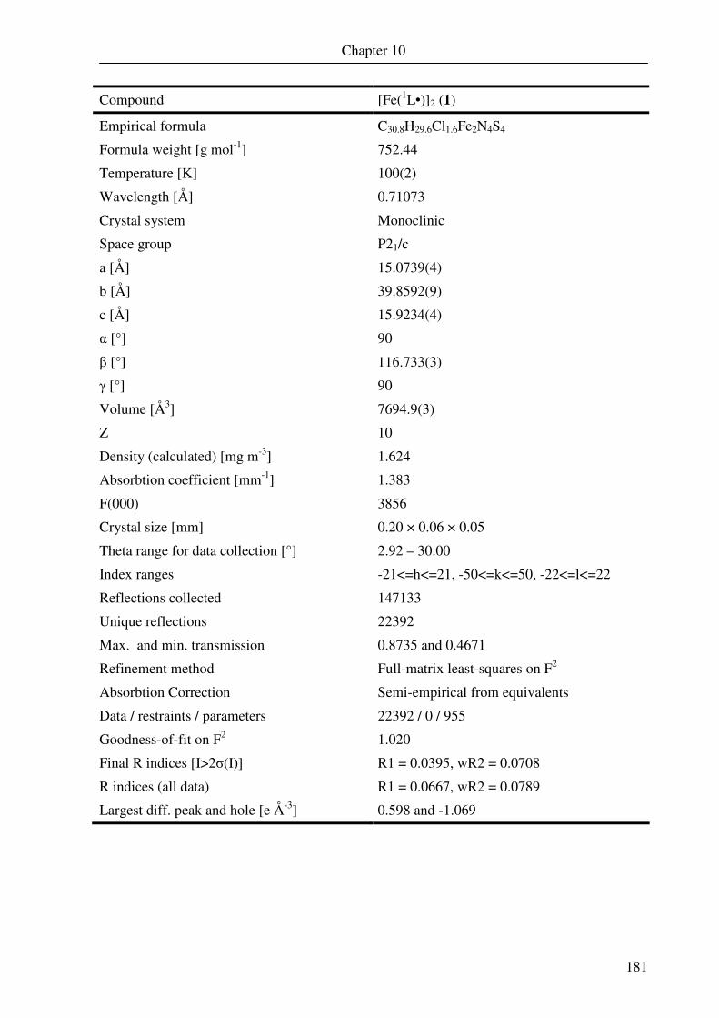
Chapter 10
181
Compound [Fe(1L•)]2 (1)
Empirical formula C30.8H29.6Cl1.6Fe2N4S4
Formula weight [g mol-1] 752.44
Temperature [K] 100(2)
Wavelength [Å] 0.71073
Crystal system Monoclinic
Space group P21/c
a [Å] 15.0739(4)
b [Å] 39.8592(9)
c [Å] 15.9234(4)
α [°] 90
β [°] 116.733(3)
γ [°] 90
Volume [Å3] 7694.9(3)
Z 10
Density (calculated) [mg m-3] 1.624
Absorbtion coefficient [mm-1] 1.383
F(000) 3856
Crystal size [mm] 0.20 × 0.06 × 0.05
Theta range for data collection [°] 2.92 – 30.00
Index ranges -21<=h<=21, -50<=k<=50, -22<=l<=22
Reflections collected 147133
Unique reflections 22392
Max. and min. transmission 0.8735 and 0.4671
Refinement method Full-matrix least-squares on F2
Absorbtion Correction Semi-empirical from equivalents
Data / restraints / parameters 22392 / 0 / 955
Goodness-of-fit on F2 1.020
Final R indices [I>2σ(I)] R1 = 0.0395, wR2 = 0.0708
R indices (all data) R1 = 0.0667, wR2 = 0.0789
Largest diff. peak and hole [e Å-3] 0.598 and -1.069

Chapter 10
182
Compound [Fe(2L•)]2 (2)
Empirical formula C60H88Fe2N4S4 • C6H14
Formula weight [g mol-1] 1191.46
Temperature [K] 100(2)
Wavelength [Å] 0.71073
Crystal system Monoclinic
Space group C2/c
a [Å] 26.2316(8)
b [Å] 14.7286(4)
c [Å] 18.1216(4)
α [°] 90
β [°] 110.60(1)
γ [°] 90
Volume [Å3] 6553.7(3)
Z 4
Density (calculated) [mg m-3] 1.208
Absorbtion coefficient [mm-1] 0.611
F(000) 2568
Crystal size [mm] 0.52 × 0.40 × 0.14
Theta range for data collection [°] 2.18 – 33.13
Index ranges -40<=h<=40, -22<=k<=22, -27<=l<=27
Reflections collected 95856
Unique reflections 12467
Max. and min. transmission 0.9194 and 0.7418
Refinement method Full-matrix least-squares on F2
Absorbtion correction Gaussian, face-indexed
Data / restraints / parameters 12467 / 0 / 356
Goodness-of-fit on F2 1.016
Final R indices [I>2σ(I)] R1 = 0.0311, wR2 = 0.0794
R indices (all data) R1 = 0.0388, wR2 = 0.0838
Largest diff. peak and hole [e Å-3] 0.490 and -0.604
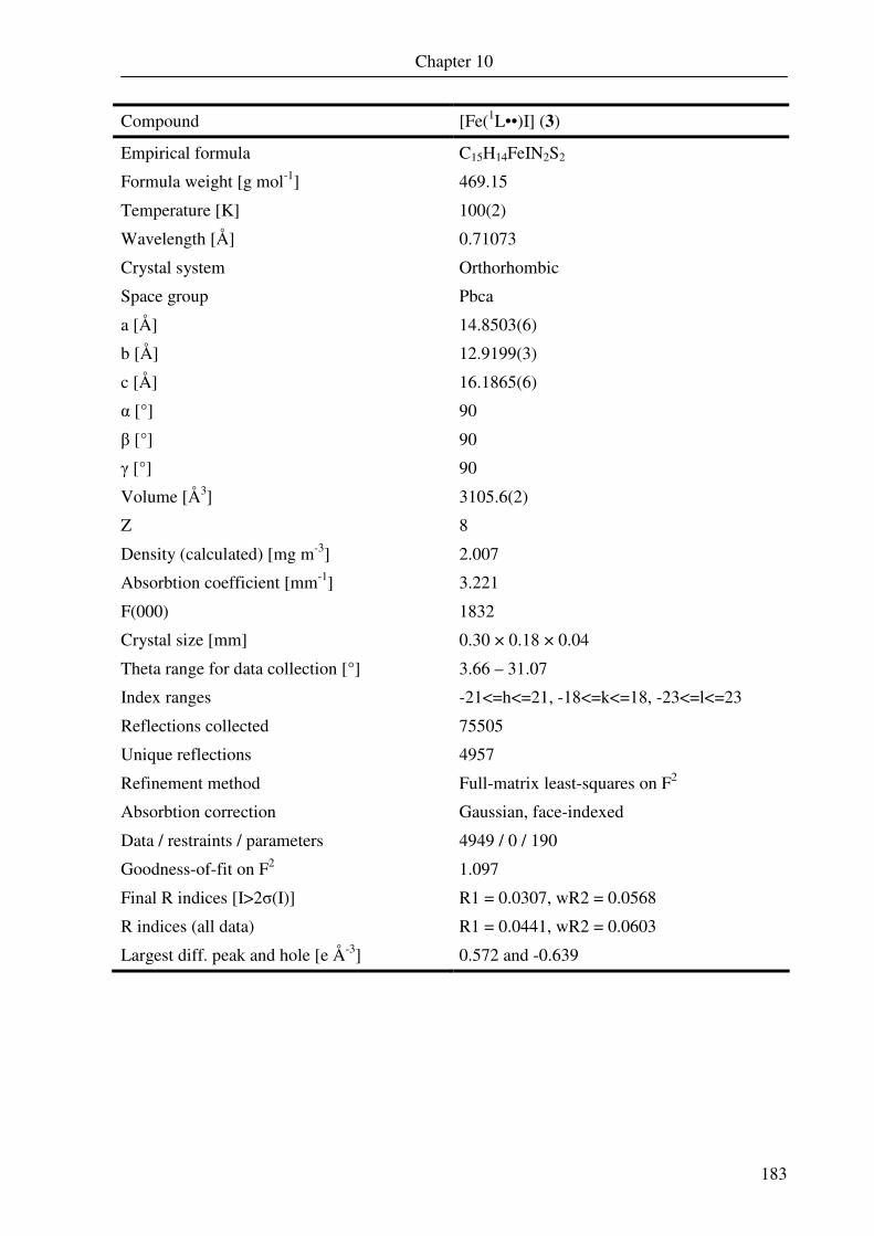
Chapter 10
183
Compound [Fe(1L••)I] (3)
Empirical formula C15H14FeIN2S2
Formula weight [g mol-1] 469.15
Temperature [K] 100(2)
Wavelength [Å] 0.71073
Crystal system Orthorhombic
Space group Pbca
a [Å] 14.8503(6)
b [Å] 12.9199(3)
c [Å] 16.1865(6)
α [°] 90
β [°] 90
γ [°] 90
Volume [Å3] 3105.6(2)
Z 8
Density (calculated) [mg m-3] 2.007
Absorbtion coefficient [mm-1] 3.221
F(000) 1832
Crystal size [mm] 0.30 × 0.18 × 0.04
Theta range for data collection [°] 3.66 – 31.07
Index ranges -21<=h<=21, -18<=k<=18, -23<=l<=23
Reflections collected 75505
Unique reflections 4957
Refinement method Full-matrix least-squares on F2
Absorbtion correction Gaussian, face-indexed
Data / restraints / parameters 4949 / 0 / 190
Goodness-of-fit on F2 1.097
Final R indices [I>2σ(I)] R1 = 0.0307, wR2 = 0.0568
R indices (all data) R1 = 0.0441, wR2 = 0.0603
Largest diff. peak and hole [e Å-3] 0.572 and -0.639

Chapter 10
184
Compound [Fe(1L••)(P(Me)3)] (5)
Empirical formula C18H23FeN2PS2
Formula weight [g mol-1] 418.32
Temperature [K] 100(2)
Wavelength [Å] 0.71073
Crystal system Monoclinic
Space group P21/c
a [Å] 18.6136(6)
b [Å] 7.3768(2)
c [Å] 14.3961(4)
α [°] 90
β [°] 109.374(3)
γ [°] 90
Volume [Å3] 1866.58(9)
Z 4
Density (calculated) [mg m-3] 1.489
Absorbtion coefficient [mm-1] 1.120
F(000) 872
Crystal size [mm] 0.20 × 0.12 × 0.04
Theta range for data collection [°] 2.99 – 32.50
Index ranges -28<=h<=28, -11<=k<=11, -21<=l<=21
Reflections collected 38904
Unique reflections 6744
Max. and min. transmission 0.9566 and 0.8071
Refinement method Full-matrix least-squares on F2
Absorbtion correction Semi-empirical from equivalents
Data / restraints / parameters 6744 / 0 / 220
Goodness-of-fit on F2 1.019
Final R indices [I>2σ(I)] R1 = 0.0317, wR2 = 0.0729
R indices (all data) R1 = 0.0440, wR2 = 0.0792
Largest diff. peak and hole [e Å-3] 0.519 and -0.764

Chapter 10
185
Compound [Fe(1L••)(P(OMe)3)]2 (6)
Empirical formula C18H23FeN2O3PS2
Formula weight [g mol-1] 466.32
Temperature [K] 100(2)
Wavelength [Å] 0.71073
Crystal system Orthorhombic
Space group Pbca
a [Å] 22.6000(7)
b [Å] 7.4711(3)
c [Å] 23.5006(7)
α [°] 90
β [°] 90
γ [°] 90
Volume [Å3] 3968.0(2)
Z 8
Density (calculated) [mg m-3] 1.561
Absorbtion coefficient [mm-1] 1.073
F(000) 1936
Crystal size [mm] 0.14 × 0.05 × 0.03
Theta range for data collection [°] 3.00 – 32.50
Index ranges -32<=h<=34, -11<=k<=11, -35<=l<=34
Reflections collected 42206
Unique reflections 7168
Max. and min. transmission 0.9685 and 0.8643
Refinement method Full-matrix least-squares on F2
Absorbtion correction Semi-empirical from equivalents
Data / restraints / parameters 7168 / 13 / 266
Goodness-of-fit on F2 1.042
Final R indices [I>2σ(I)] R1 = 0.0351, wR2 = 0.0764
R indices (all data) R1 = 0.0569, wR2 = 0.07849
Largest diff. peak and hole [e Å-3] 0.455 and -0.407
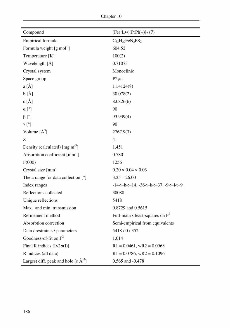
Chapter 10
186
Compound [Fe(1L••)(P(Ph)3)]2 (7)
Empirical formula C33H29FeN2PS2
Formula weight [g mol-1] 604.52
Temperature [K] 100(2)
Wavelength [Å] 0.71073
Crystal system Monoclinic
Space group P21/c
a [Å] 11.4124(8)
b [Å] 30.078(2)
c [Å] 8.0826(6)
α [°] 90
β [°] 93.939(4)
γ [°] 90
Volume [Å3] 2767.9(3)
Z 4
Density (calculated) [mg m-3] 1.451
Absorbtion coefficient [mm-1] 0.780
F(000) 1256
Crystal size [mm] 0.20 × 0.04 × 0.03
Theta range for data collection [°] 3.25 – 26.00
Index ranges -14<=h<=14, -36<=k<=37, -9<=l<=9
Reflections collected 38088
Unique reflections 5418
Max. and min. transmission 0.8729 and 0.5615
Refinement method Full-matrix least-squares on F2
Absorbtion correction Semi-empirical from equivalents
Data / restraints / parameters 5418 / 0 / 352
Goodness-of-fit on F2 1.014
Final R indices [I>2σ(I)] R1 = 0.0461, wR2 = 0.0968
R indices (all data) R1 = 0.0786, wR2 = 0.1096
Largest diff. peak and hole [e Å-3] 0.565 and -0.478

Chapter 10
187
Compound [Fe(1L••)(P(OPh)3)]2 (8)
Empirical formula C33H29FeN2O3PS2
Formula weight [g mol-1] 652.52
Temperature [K] 100(2)
Wavelength [Å] 0.71073
Crystal system Orthorhombic
Space group Pna21
a [Å] 13.0330(3)
b [Å] 24.9561(6)
c [Å] 8.7949(2)
α [°] 90
β [°] 90
γ [°] 90
Volume [Å3] 2860.57(12)
Z 4
Density (calculated) [mg m-3] 1.515
Absorbtion coefficient [mm-1] 0.769
F(000) 1352
Crystal size [mm] 0.16 × 0.07 × 0.04
Theta range for data collection [°] 3.72 – 32.50
Index ranges -17<=h<=19, -37<=k<=36, -13<=l<=13
Reflections collected 29097
Unique reflections 9241
Max. and min. transmission 0.7433 and 0.5169
Refinement method Full-matrix least-squares on F2
Absorption correction Semi-empirical from equivalents
Data / restraints / parameters 9241 / 1 / 379
Goodness-of-fit on F2 1.012
Final R indices [I>2σ(I)] R1 = 0.0362, wR2 = 0.0638
R indices (all data) R1 = 0.0531, wR2 = 0.0686
Largest diff. peak and hole [e Å-3] 0.375 and -0.338

Chapter 10
188
Compound [Fe(2L••)(P(Ph)3)]2 (9)
Empirical formula C48H59FeN2PS2
Formula weight [g mol-1] 814.19
Temperature [K] 100(2)
Wavelength [Å] 0.71073
Crystal system Triclinic
Space group P-1
a [Å] 10.4566(8)
b [Å] 14.5158(10)
c [Å] 16.4465(11)
α [°] 67.218(4)
β [°] 80.341(4)
γ [°] 74.581(4)
Volume [Å3] 2212.8(3)
Z 2
Density (calculated) [mg m-3] 1.223
Absorbtion coefficient [mm-1] 0.505
F(000) 868
Crystal size [mm] 0.04 × 0.03 × 0.006
Theta range for data collection [°] 2.98 – 22.50
Index ranges -9<=h<=11, -12<=k<=15, -17<=l<=17
Reflections collected 12277
Unique reflections 5766
Refinement method Full-matrix least-squares on F2
Absorption correction None
Data / restraints / parameters 5766 / 0 / 499
Goodness-of-fit on F2 1.037
Final R indices [I>2σ(I)] R1 = 0.0633, wR2 = 0.1158
R indices (all data) R1 = 0.1345, wR2 = 0.1484
Largest diff. peak and hole [e Å-3] 0.515 and -0.491

Chapter 10
189
Compound [Fe(2L••)(P(OPh)3)]2 (8)
Empirical formula C51.50H63FeN2O3PS2
Formula weight [g mol-1] 908.98
Temperature [K] 100(2)
Wavelength [Å] 0.71073
Crystal system Orthorhombic
Space group Pbca
a [Å] 18.0875(8)
b [Å] 16.8468
c [Å] 31.4518
α [°] 90
β [°] 90
γ [°] 90
Volume [Å3] 9583.9(8)
Z 8
Density (calculated) [mg m-3] 1.260
Absorbtion coefficient [mm-1] 0.478
F(000) 3864
Crystal size [mm] 0.14 × 0.12 × 0.07
Theta range for data collection [°] 2.97 – 27.50
Index ranges -22<=h<=23, -21<=k<=21, -40<=l<=40
Reflections collected 67364
Unique reflections 10953
Max. and min. transmission 1.0000 and 0.7266
Refinement method Full-matrix least-squares on F2
Absorption correction Semi-empirical from equivalents
Data / restraints / parameters 10953 / 5 / 577
Goodness-of-fit on F2 1.170
Final R indices [I>2σ(I)] R1 = 0.0566, wR2 = 0.1013
R indices (all data) R1 = 0.0856, wR2 = 0.1114
Largest diff. peak and hole [e Å-3] 0.638 and -0.462
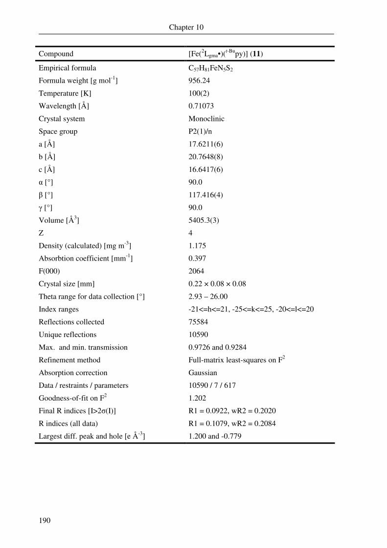
Chapter 10
190
Compound [Fe(2Lgma•)(t-Bupy)] (11)
Empirical formula C57H81FeN5S2
Formula weight [g mol-1] 956.24
Temperature [K] 100(2)
Wavelength [Å] 0.71073
Crystal system Monoclinic
Space group P2(1)/n
a [Å] 17.6211(6)
b [Å] 20.7648(8)
c [Å] 16.6417(6)
α [°] 90.0
β [°] 117.416(4)
γ [°] 90.0
Volume [Å3] 5405.3(3)
Z 4
Density (calculated) [mg m-3] 1.175
Absorbtion coefficient [mm-1] 0.397
F(000) 2064
Crystal size [mm] 0.22 × 0.08 × 0.08
Theta range for data collection [°] 2.93 – 26.00
Index ranges -21<=h<=21, -25<=k<=25, -20<=l<=20
Reflections collected 75584
Unique reflections 10590
Max. and min. transmission 0.9726 and 0.9284
Refinement method Full-matrix least-squares on F2
Absorption correction Gaussian
Data / restraints / parameters 10590 / 7 / 617
Goodness-of-fit on F2 1.202
Final R indices [I>2σ(I)] R1 = 0.0922, wR2 = 0.2020
R indices (all data) R1 = 0.1079, wR2 = 0.2084
Largest diff. peak and hole [e Å-3] 1.200 and -0.779


![Chem. Eur. J. 2010 16, 10971 10974 · 1 Chem. Eur. J. 2010, 16, 10971 – 10974 Non-innocent Behaviour of Dithiocarboxylate Ligands Based on N-heterocyclic Carbenes Saira Naeem,[a]](https://img.dokumen.tips/doc/110x75/5f79787ed5f93223856662bf/chem-eur-j-2010-16-10971-10974-1-chem-eur-j-2010-16-10971-a-10974-non-innocent.jpg)