An experimental investigation of a state-variable modal ...feeny/FarooqFeenyJVA12.pdf · An experimental investigation of a state-variable modal decomposition method for modal analysis

An experimental investigation of a state-variablemodal decomposition method for modal analysis

Umar FarooqDynamics and Vibrations Research Laboratory

Department of Mechanical EngineeringMichigan State University

E. Lansing, Michigan, 48824Email: [email protected]

B. F. Feeny∗

Department of Mechanical EngineeringMichigan State University

E. Lansing, Michigan, 48824Email: [email protected]

Phone: 517-353-9451Fax: 517-353-1750

ABSTRACTThis work presents the experimental evaluation of the state-variable modal decomposition (SVMD) method for

modal parameter estimation of multi-degree-of-freedom and continuous vibration systems. Using output responseensembles only, the generalized eigenvalue problem is formed to estimate eigen frequencies and modal vectorsfor a lightly damped linear clamped-free thin experimentalbeam. The estimated frequencies and modal vectorsare compared against the theoretical system frequencies and modal vectors. Satisfactory results are obtained forestimating both system frequencies and modal vectors for the first five modes. To validate the actual modes fromthe spurious ones, modal coordinates are employed that together with frequency and vector estimates substantiatethe true modes. The paper also addresses the error associated with estimation when the number of sensors is lessthan the active/dominant modes of the system shown via a numerical example.

1 IntroductionOutput-only modal analysis has gained popularity over recent years (for example [1–10]). Advantages of output-only

analysis over traditional modal analysis are the following. I) In many real life applications, the nature of excitationpreventsits measurement (for instance earthquake, wind, or traffic loads on structures), and output-only analysis eliminates the needto measure inputs. II) The construction of complex frequency response functions or transfer matrix functions requiresan experienced engineer to correlate various response rows(or columns) to correctly identify the system modes, and iscumbersome in cases when the modes are not well separated. III) Contrary to traditional modal analysis, in many casesoutput-only analysis can eliminate the need for stand-alone testing of the structure at various locations (or components).

Output-only methods can be either time or frequency based. Anon-exhaustive list of time domain output-only meth-ods includes the Ibrahim time domain method [1], polyreference method [2], eigensystem realization algorithm [3, 11],

∗Address all correspondence to this author.

VIB-09-1306 Farooq and Feeny 1

least square complex exponential method [4], which is similar to Prony’s method [12–14], independent component analy-sis [15, 16], and stochastic subspace identification methods [5]. Frequency based output-only methods include the orthogonalpolynomial methods [6, 7], complex mode indicator function[8], and frequency domain decomposition [9].

Recent additions to the time domain output-only family are the smooth orthogonal decomposition (SOD) [17–19] andthe state-variable modal decomposition (SVMD) [20, 21], which have shown good results for modal analysis of free responsesimulations. These methods are variants of proper orthogonal decomposition methods recently studied for structural modalanalysis [22–26]. The advantages of using these decomposition-based methods are that they do not involve the possibility ofoversized state matrices and their spurious modes (as in Ibrahim time domain and Prony’s method), estimation of states (forinstance in stochastic subspace identification methods) orspectral density functions (as in frequency domain decomposition),or constructing generalized block Hankel matrices (as in eigensystem realization algorithm), and thereby are simplerinconstruction and induce minimum assumptions.

In the previous works [20, 21], it was shown that for low noisecases, the SVMD method works very well in estimatingmodal parameters for simulations with free response and, insome cases, response to random excitations. However, toimplement the SVMD method in the real life applications, an experimental study must be conducted. The study would behelpful in understanding practical aspects of the estimation problem, for instance, proper selection of system model order,issues surrounding the number of sensors, linearity, boundary conditions, and effects of filtering. The experimental studiesconducted here address both the advantages and the limitations of applying the SVMD under the mentioned circumstances.This work thus deals with experimental verification of the ideas presented in the previous works.

We will begin by stating the assumptions for experiments. Next we will briefly revisit the SVMD method. Then we willdescribe a clamped-free beam experiment that presents a structural system modeled as an Euler-Bernoulli beam. Practicalaspects of data length and effects of filtering are addressed, followed by the use of modal coordinates for establishing true orspurious modes. Finally, we will highlight the limitationson using the SVMD method before we summarize our findings.

2 The state-variable modal decompositionIn this section, we summarize the state-variable modeling of vibration systems. The decomposition strategy is presented,

and then tied to the state-variable model.

2.1 AssumptionsWe assume the system is linear, time invariant, and has no poles in the right half plane such that techniques of system

estimation and control are applicable [27–35]. These conditions are generally necessary for calculating any frequencyresponse functions (FRFs) and hence are applicable to the output-only methods’ experimentation as well.

2.2 State-variable linear vibration modelThe state-variable model of linear vibration systems is used on systems with nonproportional (non-Rayleigh [36]) and

nonmodal (non-Caughey [37]) damping to obtain damped vibration modes [38, 39]. The equations of motion for free vibra-tions are

Mx+Cx+Kx = 0 (1)

wherex is ann×1 array of mass displacements,M ,C, andK , are then×n mass, damping, and stiffness matrices, and thedots indicate time derivatives. Then defining a 2n×1 state vectoryT = [xT ,xT ], and introducing the equationMx−Mx = 0(following Meirovitch [38, 40]), yields unforced equations of motion of the form

Ay+By = 0, (2)

where

A =

[

0 MM C

]

, B =

[

−M 00 K

]

. (3)


A andB are 2n×2n and symmetric, but are neither positive nor negative definite. (Using the formx− x = 0 in lieu of thefirst part in Eq. (2) would work as well, but would not produce the symmetry in matrixA.)

Assuming a response of the formy = eαtφ, the eigenvalue problem

αAφ+Bφ = 0 (4)

in general yields complex eigenvaluesα and eigenvectorsφ, with φ = [vT ,wT ]T , wheren×1 vector partitionv correspondsto characteristic shapes of velocity states, and partitionw represents characteristic shapes in displacement (complex modes).By the construction ofy, v = αw. The vectorsφ are orthogonal with respect to matricesA andB. The latter does not implythat the vectorsw are orthogonal with respect toM andK .

2.3 Decomposition strategyThe decomposition strategy [20], is based on the free-response state-variable ensembleY = [VT ,XT ]T , whereX is an

n×N displacement ensemble andV is then×N velocity ensemble, andW = [AT ,VT ]T , whereA is then×N accelerationensemble, whereN is the number of time samples. The “correlation” matricesR = YYT/N andN = YWT/N are thenformed.

In previous formulations of SVMD and SOD [17], then×N matrix X was assumed to be available, and the matrixVwas obtained by simple numerical differentiation, such that V = XDT

≈ X approximates the velocity ensemble. An exampleof an(N−2nd)×N matrixD of centered finite differences, withnd = 1 for half the span of the finite difference, is

D =1

2∆t

−1 0 1 0 . . . 00 −1 0 1 . . . 0...

..... .

. . .. . .

...0 . . . . . . −1 0 1

, (5)

where∆t represents the sampling time. ThusV is n× (N−2nd), and so the first and lastnd columns ofX are dropped so thatY has compatible partitions. We would then take the derivative W = YDT

≈ Y, this time using an(N−4nd)× (N−2nd)difference matrixD. The first and lastnd time samples ofY are then dropped so that the dimensions ofY andW are both2n×N−4nd. We then form the correlation matrixR = YYT/(N−4nd) and a nonsymmetric matrixN = YWT/(N−4nd).

But there may be other ways to obtain these ensembles. For example, if structural vibrations are sensed with accelerom-eters, the acceleration ensemble is sampled directly, and the velocity and displacement ensembles are obtained by carefulnumerical integration of the acceleration signals.

GivenR andN, the 2n×2n eigenvalue problem is then

αRψ = Nψ, (6)

which can be rewritten asαYYTψ = YWT ψ. Making use of Eq. (2),W ≈ Y = −A−1BY, and we have

αYY Tψ ≈−YYTBTA−Tψ. (7)

We expectYYT to be invertible. This is true if all displacement measurements are independent and ifN−4nd > n.As such,αψ ≈−BTA−Tψ. In matrix form

ΨΛ ≈−BTA−TΨ, (8)


whereΛ is a diagonal matrix of eigenvalues. Taking the inverse-transpose,Ψ−TΛ−1≈ −B−1AΨ−T , whenceBΨ−T

≈

−AΨ−TΛ, and hence

−A−1BΨ−T≈ Ψ−TΛ. (9)

LettingU = Ψ−T , the data eigenvalue problem leads to

−A−1BU ≈ UΛ, (10)

which is a generalized eigenvalue problem with matricesA andB, the solution of which determines the unknownsU andΛ.The matrix form of the structural eigenvalue problem of Eq. (4) is

−A−1BΦ = ΦΓ, (11)

a generalized eigenvalue problem with the same matricesA andB, the solution of which determines the unknownsΦ andΓ.The eigenvalue problems of Eqs. (10) and (11) have the same solution (within the modal normalization constants), indicatingthatΦ ≈ U = Ψ−T andΓ = Λ.

Ψ andΛ are 2n×2n matrices, corresponding to 2n eigenvectors and 2n eigenvalues, for ann-degree-of-freedom system.If the eigenvectors are complex, they come in conjugate pairs. That is, a conjugate pair of eigenvectors and eigenvaluesrepresents one mode. If the eigen solution is real, an eigenvector characterizes a response configuration decaying at a ratecontained in the corresponding eigenvalue. If, in fact, thedamping is “modal” (Caughey), there will ben independentdisplacement partitionsv among the 2n eigenvectors, which correspond to then more familiar synchronous normal modes.

Thus, we expect the eigenvalues of Eq. (6) to approximate thestate-variable eigenvalues, containing information aboutdamping and frequency. The inverse of the modal matrix from Eq. (6) resembles the complex linear normal modal matrix ofthe state-variable system Eq. (4), and contains velocity and displacement partitions. The only approximation in the method isin estimatingX ≈ XDT andY ≈ YDT , or in estimatingX andV by integratingA (or using a combination of these processesif V is measured). Hence we expect reasonable estimations when noise is limited and the step size is sufficiently smallcompared to characteristic time scales.

3 Clamped-free beam experimentThis section describes the modal parameter estimation of a clamped-free beam using the SVMD method for a free

vibration experiment. The system is assumed to follow the assumptions described in Section 2.1. The experimental setupofthe system is described as below.

A 941×52×3 mm3 clamped-free uniform steel beam as shown in Fig. 1 was prepared for the experiment conducted inthe Dynamics and Vibrations Research Lab at Michigan State University. The beam was sensed with 16 PCB model number352B10 accelerometers, each of which weighs 0.7 gm with a sensitivity listed in catalogue at about 10 mV/g (individualsensitivities vary slightly), equally spaced from clamp tothe beam tip. These accelerometers were bonded to the beam viabeeswax [12]. The beam properties were: elastic modulusE = 190× 109 GPa, densityρ = 7500 Kg/m3, mass per unitlength (including the sensor masses)m= 1.1907 Kg/m, (without the sensor masses ¯m= 1.1787 Kg/m, but the sensor masseswere included when calculating the theoretical natural frequencies of the system), and cross-sectional area moment ofinertiaI = 1.17×10−10 m4. Measurement signals from the accelerometers passed through signal conditioning amplifier PCB Modelnumber 481A02, the output of which was then fed to a data acquisition system (TEAC GX-1 Integrated Recorder) wherethe acceleration measurement signals were processed through a low pass filter and then converted into ASCII.txt format forrecording. Further processing of these files was done in Matlab.

The data were sampled at a rate ofFs = 5 kHz. The data were digitally filtered with the cut-off frequency of the low-pass filter set at 0.4 kHz. This value was set well below the Nyquist frequency to avoid aliasing effects. The beam wasexcited with an impulse applied between the second and thirdsensor locations, with the resulting response monitored bythe accelerometers. A superposition of accelerometer snapshots, plotted with lines to interpolate accelerations along the


beam between the accelerometers, is shown in Fig. 2. The measurement recording time was approximately 7.2 seconds,corresponding toN = 36,327 samples. The data were also high-pass filtered to reduce the low frequency noise effects onsubsequent integrations of the acceleration signals. For uniformity, each acceleration signal was then individuallycalibratedper its accelerometer sensitivity specifications. The magnitude of the fast Fourier transform (FFT) of one of the accelerationsignals is plotted in Fig. 3.

The ensemble matrix of acceleration time historiesA of size 16×N was formed. Using the Matlab routine “cumtrapz”,the velocityV and displacementX ensembles were obtained by numerical integration. All ensembles were processed toremove the respective means. Next, the correlation matrices YYT = R×N and YWT = N×N, for the decompositionmethod SVMD were formed, whereY = [VT ,XT ]T andW = [AT ,VT ]T .

3.1 Filtering effectsTo remove a low frequency “drift” in the integrated signal ensembles, data were high-pass filtered at a filter frequency

of 1.4 Hz. This value was selected at about half of the first natural frequency obtained from the FFT plot of Fig. 3. Note thatthe filter frequency was evaluated in the range of 0.5 Hz to 2.0Hz with no significant change observed in the high frequencyestimates, and some improvements were seen in the lowest frequency estimate as the filter frequency approached to 0.5 Hz.This suggests that as a limiting case, a maximum of one half ofthe fundamental frequency by FFT should be employed asthe filter corner frequency.

The frequency response of the second-order high-pass filtermodeled as a single-degree-of-freedom system is shown inFig. 4. The filter amplitude at twice the break frequency is observed to be 0 dB, thus implying that application of the filterdoes not reduce the component amplitudes of the estimated frequencies. The phase shifting effects caused by this filter canbe removed by running the filter “backwards”. In that way, thefilter becomes a fourth order system.

The filter is applied prior to, and after each numerical integration of the signals. Thus, to maintain consistency, theacceleration ensemble should be filtered thrice, the velocity ensemble twice and the displacement ensemble only once. Castthis way, the filter order becomes 12 for the ensembles.

A reviewer suggested that these filtering issues could be avoided by differentiating the acceleration twice, instead ofintegrating, to formY = [DAT ,AT ]T andW = YDT , from which the eigenvalue problem could be formulated. Indeed, thismight be possible for free vibrations, as two derivatives ofthe homogeneous equation of motion Eq. (2) yield an equationof the formA

...y +By = 0. As such, the eigenvalue problem so formulated should be connected to this equation by the same

development as in Section 2.3. While this approach would avoid integration drift and high-pass filtering, and might be worthinvestigating, differentiation also could excessively amplify high-frequency noise and overly emphasize high frequencycomponents of the response.

3.2 Identification resultsWe initially kept the firstN = 12,000 samples to minimize the contribution of the high frequency noise that dominated

the later part of the decayed signal ensembles. These reduced sized ensemble matricesY andW were then assembled into theSVMD eigenvalue problem from which the eigenvectors and eigenvalues were extracted. From the acceleration snapshots inFig. 2, we see that the beam acceleration had a dominant second mode, implying that the impulse input, or equivalently theinitial conditions, had a stronger effect on the second modal coordinate acceleration than the rest [38].

The theoretical frequency values and the values from takingthe FFT and log decrement method are tabulated in Table 1for the first two modes. The logarithmic decrement method wasapplied to carefully excited, dominantly single-mode ex-citation responses (obtained by constraining a nodal pointwhile plucking the beam). The SVMD method identified modalfrequencies and the respective damping ratios as also presented the same table. The error thus in the frequency estimates is1.41% and 0.30% respectively.

Since the high frequency modes are expected to damp out rather quickly, for the same experimental response, in orderto see higher modes, data were further pared down to the firstN = 1000 points. Then the decomposition method wasable to estimate the first five modes. The obtained frequency identification results for the first five modes are shown in the


Table 2. Damping estimates for the first three modes were again computed on the carefully excited, dominantly “pure mode”responses by the log decrement method and are compared against the identification scheme in the Table 3.

It is clear from these two (N = 12,000 andN = 1000) data sets that a trade-off exists between the number ofmodesto be estimated and the accuracy acquired from the estimation. For an estimation of lower modes, a large-time data set isexpected to be useful since higher modes generally dissipate quickly, leaving lower modes to dominate most of the recordedresponse. On the other hand, for the estimation of higher modes, a relatively short-time data set could be utilized with thecaveat that the “short-time” data set begins to err in the lower modal parameter estimates if the time record is short comparedto the lower modal periods. This can be observed in the damping estimate of the first mode that was completely “missed” bythe decomposition method even though the frequency estimate for that mode remains reasonable.

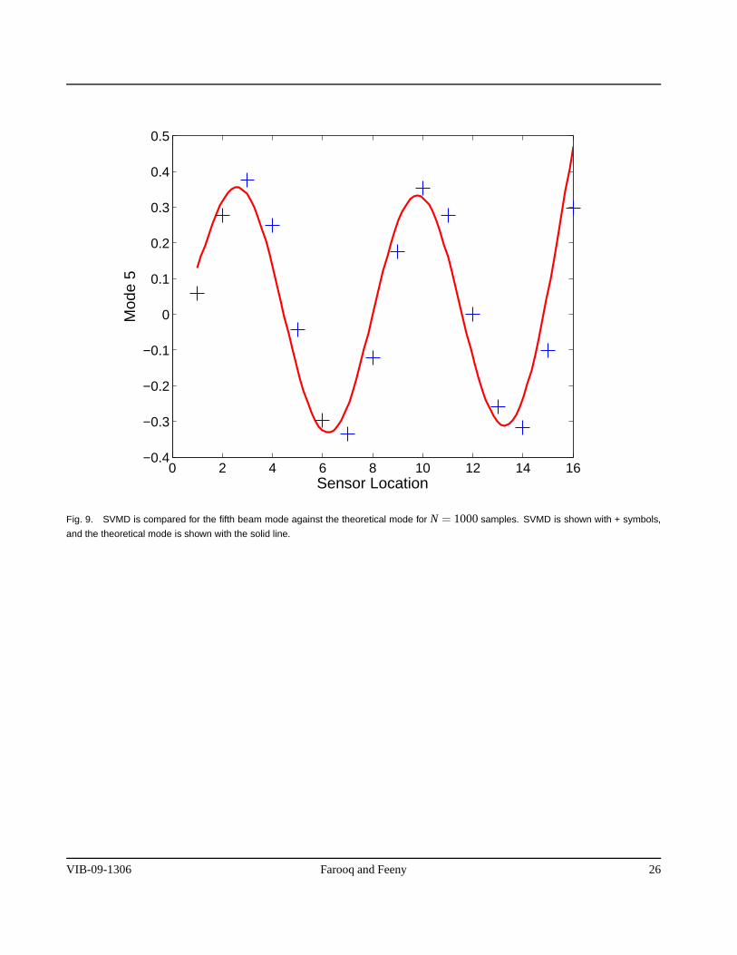
Mode shapes were then estimated using the SVMD method using the N = 1000 sample points. The eigenvectorsobtained from the method were normalized and are plotted separately for each mode in the Figures 5, 6, 7, 8, and 9. Thesemodal vectors and frequency estimates accord with the theoretical modes with a distortion observed in the lowest mode. Thisdistortion is speculated to be due to low frequency limit on the PCB sensor (per product specs, sensor’s working range is2-10,000 Hz, the lower limit being close enough to the fundamental frequency of the beam).

In both the long and short time-record examples, the number of identified modal sets is well less than the number,n, ofsensors. The remaining identified modes are spurious. The spurious modes are distinct from the estimated true modes andtheir complex conjugate pairs, and are dominated by noise. The extraction of shapes of higher modes is expected to improvefor shorter time records, similar to the trend with the frequency and damping estimates.

It is conceivable that spurious SVMD frequencies could be similar to the true frequencies. In this case, the quality ofmodal coordinates may give a clue to which modes are true.

3.3 Modal coordinatesThe POD uses proper orthogonal modal coordinates (POCs) to determine the modal frequencies and which modes

correspond to which frequencies, as explained in detail in references [22, 41]. To this end, the state-variable vector can bewritten as

y(t) =n

∑i=1

qi(t)φi, (12)

whereqi(t) are the modal-coordinate state variables. Sampled state variables can be written in matrix-ensemble form asY = ΦQ, whereΦ = Ψ−T from the SVMD eigenvalue problem (6), and elements in theith row ofQ are theith “state variablemodal coordinates” (SVMCs), which approximate the sampledmodal-coordinate state-variable historiesqi(t). Thus, modalcoordinatesQ are simply estimated by

Q = Φ−1Y = ΨTY, (13)

whereΦ approximates the state-variable linear normal modal matrix via Ψ, which is obtained by directly solving the SVMDeigenvalue problem (6).

Modal coordinates for the SVMD, the SVMCs, are presented in Fig. 10. It was shown [22, 41] that the POD directlyyields modal dominance and that proper orthogonal modal coordinates give information on modal frequencies. While SVMDgets frequency and damping estimates directly, modal coordinates can indicate the quality of decomposition. As a verification


step, frequencies can usually be estimated from modal coordinate histories either in the time domain or frequency domain. Inour beam experiment, however, withN = 1000, the first modal coordinate time history was not long enough to capture muchmore than a half period of first modal coordinate oscillation(although SVMD was still able to extract this mode). But thehigher modes had sufficient modal oscillations to easily estimate frequencies from the modal coordinates. Fig. 10 suggeststhat small amounts of lower modes have have leaked into the higher-modal coordinate histories, thus showing a significantlow-frequency perturbation on these signals, especially in the mode 3 and mode 4.

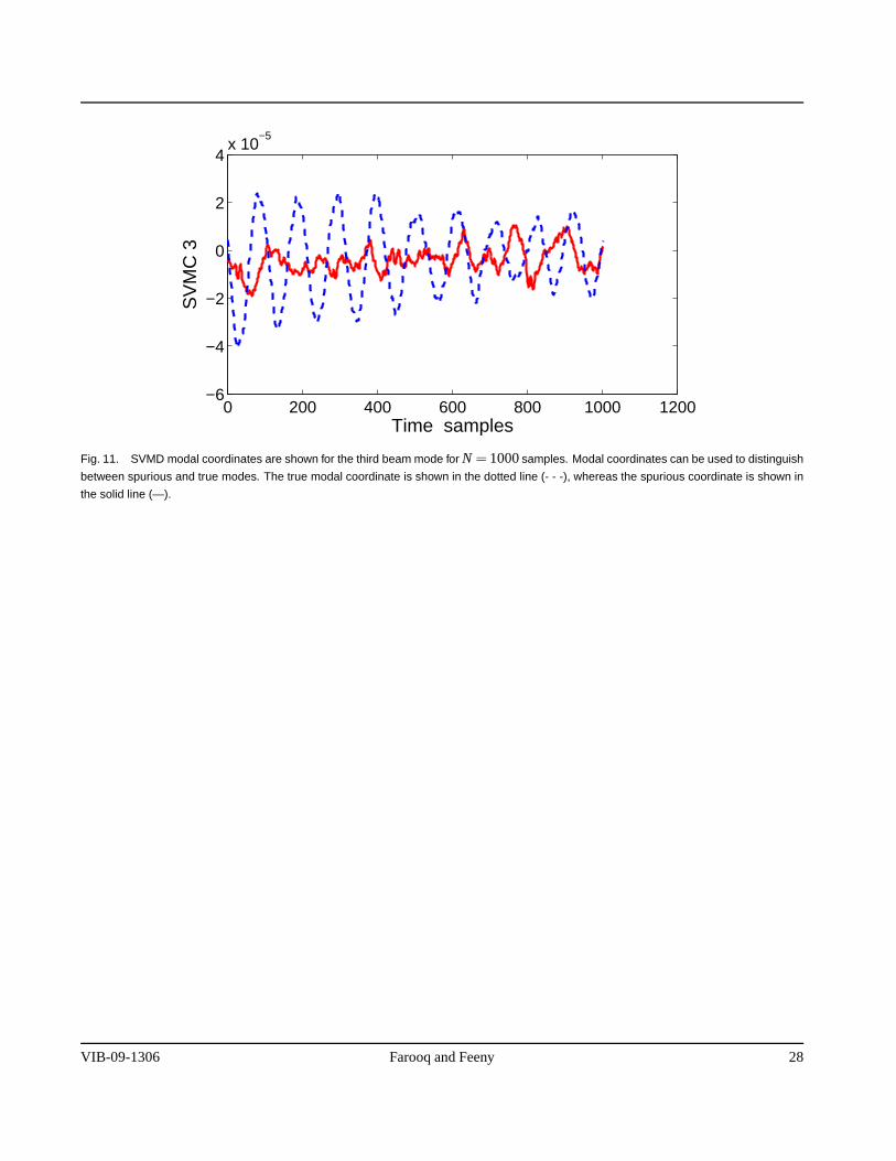
With the exception of maybe the fourth mode, coordinates aresmoothly shaped. A smooth periodic non-noisy modalcoordinate history can intuitively indicate a true mode. For the fourth mode, the latter half of the modal coordinate historyis distorted by noise. But the first half is good, so it is stilla candidate of a true mode. Thus, the first half of fourth SVMCwas tested, together with Fig. 8 and the frequency estimatedby SVMD, it was concluded to be a true system mode. Also, ifspurious frequencies are estimated by the SVMD, modal coordinates can help determine the true modes from fictitious ones.As an example, this is seen in Fig. 11 where modal frequenciesestimated by the SVMD are close (47.39 and 44.81 Hz), butthe modal coordinates clearly indicate the noisy, hence thespurious modal coordinate (shown in the figure as the solid line).

4 Limitations on the number of sensors and active modesIn the theoretical development of the SVMD method, it was implicitly assumed that a sufficient number of measurement

sensors were always available for obtaining the time seriesdata for modal parameter estimation. This number should begreater than or equal to the number of system frequencies present in the response. In real systems, however, only a limitednumber of sensors can be applied regardless of the number of active degrees of freedom. We observed in Sec. 3 the casewhen more sensors were available than there were active modes. In this case, SVMD was able to extract a fairly large numberof dominant true modal parameters (in addition to generating spurious modal estimations). In a situation, though, where thenumber of available sensors would be less than the active (dominant) system modes, the SVMD may run into problems. Tosee this, we will conduct a sensitivity analysis followed bya numerical simulation in the following sections.

4.1 Sensitivity analysisWe have seen that if the number,n, of sensors is greater than the number of true active modes, spurious modes are

present. Conversely, if the number of sensors employed for identification is less than active/dominant frequencies present inthe system, the identified frequencies may deviate from the actual frequencies. To explore this, in this section we analyzea harmonic oscillation that is contaminated by a small amplitude perturbation harmonic term with only one sensor beingused by the system. We are interested in the conditions underwhich the SVMD identification of the harmonic signal wouldproduce results with minimum or (in ideal case) no estimate deviations. The analysis is carried out by constructing theSVMD eigenvalue problem by this under-sensed system and by obtaining an approximate solution of system eigenvalues.

Consider a response signal containing two harmonic terms offrequenciesω1 andω2 such that the amplitudeA2 of theharmonic of frequencyω2 is very small as compared to the amplitudeA of the harmonic of frequencyω1, i.eA2 = εA. Then

x(t) = Acosω1(t)+ εAcosω2(t) (14)

Taking the derivative twice, we obtain

x(t) = −ω1Asinω1(t)− εAω2sinω2(t) (15)

x(t) = −ω21Acosω1(t)− εAω2

2cosω2(t) (16)

Forming they(t) andy(t) vectors, we get


y(t) =

[

xx

]

=

[

−ω1Asinω1t −ω2εAsinω2tAcosω1t + εAcosω2t

]

(17)

y(t) =

[

xx

]

=

[

−ω21Acosω1t −ω2

2εAcosω2t−ω1Asinω1t −ω2εAsinω2t

]

(18)

Thus, the key matricesy(t)y(t)T andy(t)y(t)T are obtained as

y(t)y(t)T =

ω21A2sin2 ω1t

+ω22ε2A2sin2 ω2t

+2ω1ω2εA2sinω1t sinω2t

−ω1A2sinω1t cosω1t

−ω1εA2sinω1t cosω2t


−ε2ω2A2sinω2t cosω2t





A2cos2 ω1t

+ε2A2cos2 ω2t

+2εA2cosω1t cosω2t

and

y(t)y(t)T =

ω31A2sinω1t cosω1t

+ω22ω1εA2sinω1t cosω2t

+ω32ε2A2sinω2t cosω2t

+ω21ω2εA2sinω2t cosω1t

ω1A2sin2 ω1t

+ω22ε2A2sin2 ω2t

+2ω1ω2εA2sinω2t sinω1t

−ω21A2cos2 ω1t

−ω22εA2cosω1t cosω2t

−εω21A2cosω1t cosω2t

−ω22ε2A2cos2 ω2t





We relate they(t)y(t)T andy(t)y(t)T to YYT andYWT by approximating the summations inYYT∆t andYWT∆t asintegrals on elements ofy(t)y(t)T andy(t)y(t)T . Integrating, making use of trigonometric identities, applying to the SVMDeigenvalue problem (6), and simplifying, we obtain

ω21A2 + ω2

2ε2A2

20

0A2 + ε2A2

2

ΨΛ (19)

=

0(ω2

1A2 + ω22ε2A2)

2

−

(ω21A2 + ω2

2ε2A2)

20

Ψ


which further simplifies to

ΨΛ =

0 1

−

(ω21A2 + ω2

2ε2A2)

(A2 + ε2A2)0

Ψ =

0 1

−

(ω21 + ω2

2ε2)

(1+ ε2)0

Ψ (20)

The identified eigenvalues of this system are

λ = −

(ω21 + ω2

2ε2)

(1+ ε2)(21)

We observe that if the perturbation amplitude is small, thatis if ε ≈ 0, then the eigenvalues are approximatelyω21 and the

SVMD correctly identifies the system frequency. However, ifε is significant, the eigenvalues estimation suffers greatly. Thiswould be the case where either the system may have high noise amplitudes, or the system may have many active/dominantmodes such that the harmonic amplitudes cannot be correlated (i.eA andA2 are independent, as opposed to the assumptionmade earlier in this analysis where harmonic amplitudes were related).

Addition of a third frequency perturbation of strengthε3 to the original signal approximately results inλ2 =−

(ω21 + ω2

2ε2 + ω23ε2

3)

(1+ ε2+ ε23)

,

that further deviates the SVMD identification from the actual frequency.This analysis is of this simple signal illustrates the repercussions of having limited availability of the sensor numbers

and significance of low amplitude noise on the signals when using the SVMD for modal parameter identification. Next, wewill present a more complicated numerical example.

4.2 Numerical ExampleIn this example, we simulated the numerical three-degree-of-freedom mass-spring-damper example using modal damp-

ing (c = 0.01M) shown in [22] with the difference of having an additional perturbation harmonic in the system as explainedbelow.

The computation usedN = 2000 data points, with time step∆t = 0.01, was corrupted with 8 bit quantization noise, andused a differentiation step size of 32 (nd = 16) [20, 21]. The response was constructed fromy(t) = Φq = Φq0eαt whereq0 = ΦTAy(0).

While constructing the modal coordinatesq(t), we added a perturbation harmonic of frequencyω = 2ω3, with anamplitudeε = 0.1 to the third modal signal. In this way, the system had a fourth frequency, effectively from an unmodeledmode, with only three sensors. The estimated parameters areshown in Table 4.

Modal identification of the first two modes was very good. We see that the third mode was “off”. The approximationof Eq. (21) estimates the undamped system frequency atω3e = 1.7048, which was not quite achieved due to presence ofdamping and additional degrees of freedom in the system. (When we ran a simulation for undamped case, SVMD estimatedω3 = 1.7483 which is closer to the predicted value). Also in general, increase in the noise amplitude resulted in increasederror in estimates.

It is clear from this simulation study that the decomposition method at best, is only as good as the number of sensorsavailable to it.

5 ConclusionWe have experimentally evaluated the modal parameter identification of structural systems using the state-variable modal

decomposition method on a thin beam. It is possible that our experiment has some deviation from standard assumptions suchas linearity, time invariance and ideal boundary conditions, and as such the identification can have some errors. The identifiedsystem was matched against the theoretical results of an Euler beam.

The decomposition method showed good results for modal parameter identification. For the beam, a greater numberof sensors was used than the active/dominant frequencies present in the system and the system frequencies, damping ratios


and mode shapes were obtained. We observed that data length can be slightly manipulated to either identify greater numberof modes or increase accuracy in lower modal identification.The trend observed was that short time records result inhigher-mode estimates whereas longer time records are goodfor lower-mode estimates. Some spurious modes can appearin parameter identification, and by using the modal coordinates together with the modal vectors, spurious modes can beefficiently separated. Work is is underway to quantify the quality of modal coordinates. The observations stated hereinweregained by testing multiple experimental test beams (not allshown). It was also observed that low frequency noise issuescanbe addressed by an appropriate filter selection.

This study also showed that if the number of active/dominantsystem modes is greater than the number of sensorsavailable, the SVMD method may not be able to accurately identify some of the modal parameters.

AchnowledgementsThis material is based upon work supported by the National Science Foundation under Grant No. CMMI-0727838.

Any opinions, findings, and conclusions or recommendationsexpressed in this material are those of the authors and do notnecessarily reflect the views of the National Science Foundation.

References[1] Ibrahim, S. R., and Mikulcik, E. C., 1977. “A method for the direct identification of vibration parameters from the free

response”.Shock and Vibration Bulletin,47(4), pp. 183–198.[2] Vold, H., Kundrat, J., Rocklin, G., and Russel, R., 1982.“A multi-input modal estimation algorithm for mini-computer”.

SAE Technical Papers Series, No 820194,91, pp. 815–821.[3] Juang, J.-N., and Pappa, R. S., 1985. “An eigensystem realization algorithm for modal parameter identification and

model reduction”.Journal of Guidance, Control and Dynamics,8(5), pp. 620–627.[4] Brown, D. L., Allemang, R. J., Zimmerman, R. D., and Mergeay, M., 1979. “Parameter estimation techniques for

modal analysis”.SAE Transactions, SAE Paper Number 790221,88, pp. 828–846.[5] Overschee, P. V., and De Moor, B., 1996.Subspace Identification for Linear Systems: Theory- Implementation-

Applications. Kluwer Academic Publishers, Boston.[6] Vold, H., 1986. “Orthogonal polynomials in the polyreference method”. In Proceedings of the International Seminar

on Modal Analysis, Katholieke University of Leuven, Belgium.[7] Richardson, M., and Formenti, D. L., 1982. “Parameter estimation from frequency response measurements using

rational fraction polynomials”. In Proceedings of the International Modal Analysis Conference, pp. 167–182.[8] Shih, C. Y., Tsuei, Y. G., Allemang, R. J., and Brown, D. L., 1988. “Complex mode indication function and its

application to spatial domain parameter estimation”.Mechanical System and Signal Processing,2, pp. 367–377.[9] Brincker, R., Zhang, L., and Andersen, P., 2001. “Modal identification of output-only systems using frequency domain

decomposition”.Smart Materials And Structures,10, pp. 441–445.[10] Liu, W., Gao, W.-C., and Sun, Y., 2009. “Application of modal identication methods to spatial structure using field

measurement data”.Journal of Vibration and Acoustics,131(5), p. 034503.[11] Juang, J.-N., and Phan, M. Q., 2001.Identification and Control of Mechanical Systems. Cambridge University Press,

New York.[12] Ewins, D. J., 1984.Modal Testing: Theory and Practice. Research Studies Press, Letchworth, Hertfordshire, England.[13] Braun, S., and Ram, Y. M., 1987. “Determination of structural modes via the prony model: System order and noise

induced poles”.The Journal of the Acoustical Society of America,81(5), pp. 1447–1459.[14] Arruda, J. R. F., Campos, J. P., and Pivab, J. I., 1996. “Experimental determination of flexural power flow in beams

using a modified prony method”.Journal of Sound and Vibration,197(3), October, pp. 309–328.[15] Kerschen, G., Poncelet, F., and Golinval, J. C., 2007. “Physical interpretation of independent component analysis in

structural dynamics”.Mechanical Systems and Signal Processing,21(4), May, pp. 1561–1575.[16] Poncelet, F., Kerschen, G., Golinval, J. C., and Verhelst, D., 2007. “Output-only modal analysis using blind source

separation techniques”.Mechanical Systems and Signal Processing,21, pp. 2335–2358.[17] Chelidze, D., and Zhou, W., 2006. “Smooth orthogonal decomposition-based vibration mode identification”.Journal

of Sound and Vibration,292, pp. 461–473.


[18] Zhou, W., and Chelidze, D., 2008. “Generalized eigenvalue decomposition in time domain modal parameter identifica-tion”. Journal of Vibration and Acoustics,130(1), Feb, pp. 1–6.

[19] Farooq, U., and Feeny, B. F., 2008. “Smooth orthogonal decomposition for randomly excited systems”.Journal ofSound and Vibration,316(3-5), Sep, pp. 137–146.

[20] Feeny, B. F., and Farooq, U., 2008. “A nonsymmetric state-variable decomposition for modal analysis”.Journal ofSound and Vibration,310(4-5), March, pp. 792–800.

[21] Feeny, B. F., and Farooq, U., 2007. “A state-variable decomposition method for estimating modal parameters”. InASME International Design Engineering Technical Conferences.

[22] Feeny, B. F., and Kappagantu, R., 1998. “On the physicalinterpretation of proper orthogonal modes in vibrations”.Journal of Sound and Vibration,211(4), pp. 607–616.

[23] Feeny, B. F., 2002. “On the proper orthogonal modes and normal modes of continuous vibration systems”.Journal ofVibration and Acoustics,124(1), pp. 157–160.

[24] Han, S., and Feeny, B. F., 2003. “Application of proper orthogonal decomposition to structural vibration analysis”.Mechanical Systems and Signal Processing,17(5), pp. 989–1001.

[25] Kerschen, G., and Golinval, J. C., 2002. “Physical interpretation of the proper orthogonal modes using the singularvalue decomposition”.Journal of Sound and Vibration,249(5), pp. 849–865.

[26] Feeny, B. F., and Liang, Y., 2003. “Interpreting properorthogonal modes in randomly excited vibration systems”.Journal of Sound and Vibration,265(5), pp. 953–966.

[27] Bendat, J. S., and Piersol, A. G., 1971.Random Data : Analysis and Measurement Procedures. John Wiley & Sons,New York.

[28] Bendat, J. S., and Piersol, A. G., 1986.Random Data : Analysis and Measurement Procedures, 2nd ed. John Wiley &Sons, New York.

[29] McConnell, K., 1995.Vibration Testing: Theory and Practice. John Wiley and Sons, Inc., New York.[30] Kailath, T., 1980.Linear Systems. Prentice Hall, Englewood Cliffs, NJ.[31] Rugh, W. J., 1995.Linear System Theory, 2 ed. Prentice Hall, Englewood Cliffs, NJ.[32] Chen, C.-T., 1998.Linear System Theory and Design, 3rd ed. Oxford University Press, New York, Aug.[33] Skogestad, S., and Postlethwaite, I., 2005.Multivariable Feedback Control: Analysis and Design. John Wiley and

Sons, New York, Sep.[34] Khalil, H. K., 2002.Nonlinear Systems, 3rd ed. Prentice Hall, Upper Saddle River, New Jersey.[35] Antsaklis, P. J., and Michel, A. J., 2006.Linear Systems. Birkhauser, New York.[36] Rayleigh, L., 1877.The Theory of Sound, Vol. 1. reprinted by Dover 1945, New York.[37] Caughey, T. K., 1960. “Classical normal modes in dampedlinear systems.”.Journal of Applied Mechanics,27,

pp. 269–271. Transactions of the ASME 82, series E.[38] Meirovitch, L., 1997.Principles and Techniques of Vibrations. Prentice Hall., New York.[39] Ginsberg, J., 2001.Mechanical and Structural Vibrations,. Wiley, New York.[40] Meirovitch, L., 1967.Analytical Methods in Vibrations. Macmillan, New York.[41] Feeny, B. F., 2002. “On proper orthogonal coordinates as indicators of modal activity”.Journal of Sound and Vibration,

255(5), pp. 805–817.


List of Tables1 Estimated modal parameters from the decomposition methodfor a linear beam free response compared to

the theoretical undamped Euler-Bernoulli eigen frequencies and to classical methods (FFT and single-modelogarithmic decrement) for data consisting of the firstN = 12,000 sample values . . . . . . . . . . . . . . 14

2 Experimental system frequencies (Hz.) estimated from SVMD based onN = 1000 samples of a linearbeam free response compared to the theoretical undamped Euler-Bernoulli beam eigenfrequencies and thefrequencies obtained by FFT. . . . . . . . . . . . . . . . . . . . . . . . . . .. . . . . . . . . . . . . . . . 15

3 Experimental modal damping estimated from the SVMD methodbased onN = 1000 samples of the linearfree response. Only the first three modal damping factor wereexperimentally estimated by logarithmicdecrement applied to “pure mode” responses. . . . . . . . . . . . . .. . . . . . . . . . . . . . . . . . . . 16

4 Modal parameters estimation from reduced number of sensors compared against the theoretical eigenvalueproblem from the model for a lightly damped three-degree-of-freedomdiscrete system with 8 bit quantizationnoise . . . . . . . . . . . . . . . . . . . . . . . . . . . . . . . . . . . . . . . . . . . . . .. . . . . . . . . 17


List of Figures1 The experimental setup of a clamped-free beam sensed with 16 accelerometers. . . . . . . . . . . . . . . . 182 Superposed snapshots of the 16 acceleration sample values, connected by lines across the clamped-free beam. 193 The amplitude plot of the FFT of the clamped-free beam. Onlythe first six modes are represented. . . . . . 204 The frequency response of the second order high-pass filterfor the post processing of the sensor signals. . . 215 SVMD is compared for the first beam mode against the theoretical mode forN = 1000 samples. SVMD is

shown with + symbols, and the theoretical mode is shown with the solid line. . . . . . . . . . . . . . . . . 226 SVMD is compared for the second beam mode against the theoretical mode forN = 1000 samples. SVMD

is shown with + symbols, and the theoretical mode is shown with the solid line. . . . . . . . . . . . . . . . 237 SVMD is compared for the third beam mode against the theoretical mode forN = 1000 samples. SVMD is

shown with + symbols, and the theoretical mode is shown with the solid line. . . . . . . . . . . . . . . . . 248 SVMD is compared for the fourth beam mode against the theoretical mode forN = 1000 samples. SVMD

is shown with + symbols, and the theoretical mode is shown with the solid line. . . . . . . . . . . . . . . . 259 SVMD is compared for the fifth beam mode against the theoretical mode forN = 1000 samples. SVMD is

shown with + symbols, and the theoretical mode is shown with the solid line. . . . . . . . . . . . . . . . . 2610 SVMD modal coordinates are shown for the first five beam modes based onN = 1000 samples. Modal

coordinates indicate the quality of the decomposition, andcan be used to distinguish between spurious andtrue modes. . . . . . . . . . . . . . . . . . . . . . . . . . . . . . . . . . . . . . . . . .. . . . . . . . . . 27

11 SVMD modal coordinates are shown for the third beam mode for N = 1000 samples. Modal coordinates canbe used to distinguish between spurious and true modes. The true modal coordinate is shown in the dottedline (- - -), whereas the spurious coordinate is shown in the solid line (—). . . . . . . . . . . . . . . . . . . 28


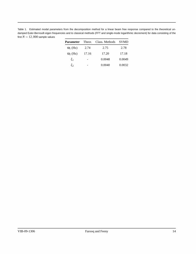
Table 1. Estimated modal parameters from the decomposition method for a linear beam free response compared to the theoretical un-

damped Euler-Bernoulli eigen frequencies and to classical methods (FFT and single-mode logarithmic decrement) for data consisting of the

first N = 12,000sample values

Parameter Theor. Class. Methods SVMD

ω1 (Hz) 2.74 2.75 2.78

ω2 (Hz) 17.16 17.20 17.18

ζ1 - 0.0048 0.0049

ζ2 - 0.0040 0.0032


Table 2. Experimental system frequencies (Hz.) estimated from SVMD based on N = 1000samples of a linear beam free response

compared to the theoretical undamped Euler-Bernoulli beam eigenfrequencies and the frequencies obtained by FFT.

Frequency Theoretical FFT SVMD

ω1 2.74 2.75 3.01

ω2 17.16 17.20 17.18

ω3 48.05 47.21 47.39

ω4 94.16 94.28 88.96

ω5 156.66 155.9 153.78


Table 3. Experimental modal damping estimated from the SVMD method based on N = 1000samples of the linear free response. Only

the first three modal damping factor were experimentally estimated by logarithmic decrement applied to “pure mode” responses.

Damping Log Decrement SVMD

ζ1 0.0048 -0.035

ζ2 0.0040 0.0040

ζ3 0.0036 0.018

ζ4 - 0.0077

ζ5 - 0.0017


Table 4. Modal parameters estimation from reduced number of sensors compared against the theoretical eigenvalue problem from the model

for a lightly damped three-degree-of-freedom discrete system with 8 bit quantization noise

Method Model SVMD

Mode (i) Freq. Damp. Freq. Damp.

Mode 1 0.4209 0.0119 0.4208 0.0125

Mode 2 1.0000 0.0050 0.9958 0.0050

Mode 3 1.6801 0.0030 1.7844 0.0054


Fig. 1. The experimental setup of a clamped-free beam sensed with 16 accelerometers.


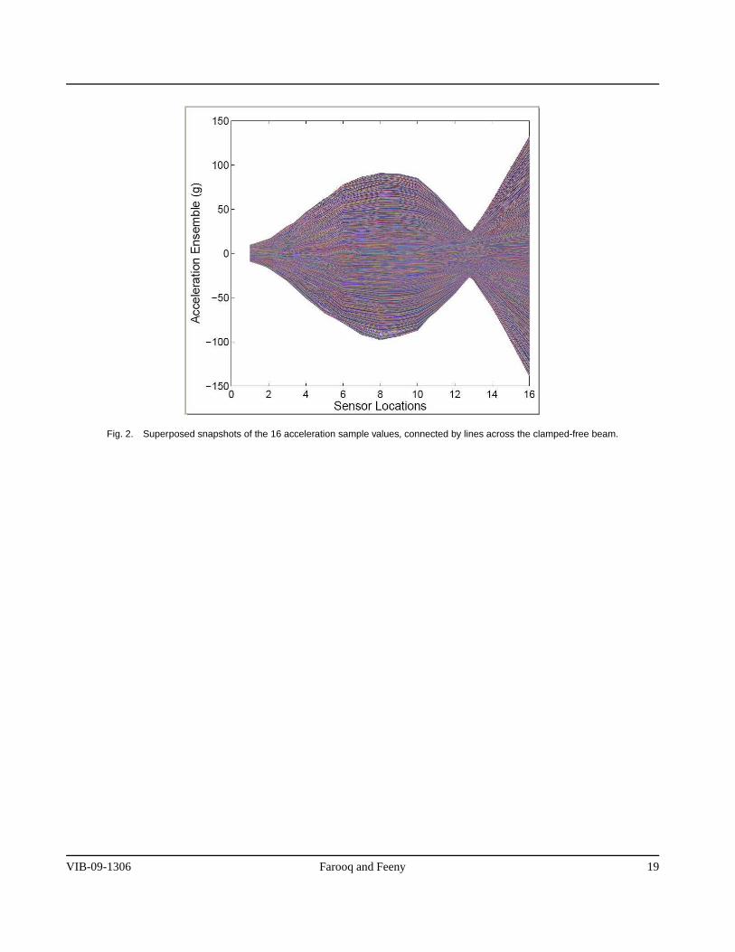
Fig. 2. Superposed snapshots of the 16 acceleration sample values, connected by lines across the clamped-free beam.


0 50 100 150 200 250 300 350

−240

−220

−200

−180

−160

−140

−120

−100

−80

−60

−40

Hz

|fft(

x)|

17.2

2.75

230.7

47.21 94.28155.9

Fig. 3. The amplitude plot of the FFT of the clamped-free beam. Only the first six modes are represented.


−80

−60

−40

−20

0

Mag

nitu

de (

dB)

10−2

10−1

100

101

102

0

90

180

Pha

se (

deg)

Frequency (Hz)

Fig. 4. The frequency response of the second order high-pass filter for the post processing of the sensor signals.


0 2 4 6 8 10 12 14 16−0.1

0

0.1

0.2

0.3

0.4

0.5

0.6

Sensor Location

Mod

e 1

Fig. 5. SVMD is compared for the first beam mode against the theoretical mode for N = 1000samples. SVMD is shown with + symbols,

and the theoretical mode is shown with the solid line.


0 2 4 6 8 10 12 14 16−0.5

−0.4

−0.3

−0.2

−0.1

0

0.1

0.2

0.3

0.4

Sensor Location

Mod

e 2

Fig. 6. SVMD is compared for the second beam mode against the theoretical mode for N = 1000samples. SVMD is shown with + symbols,



0 2 4 6 8 10 12 14 16−0.4

−0.2

0

0.2

0.4

0.6

Sensor Location

Mod

e 3

Fig. 7. SVMD is compared for the third beam mode against the theoretical mode for N = 1000samples. SVMD is shown with + symbols,



0 2 4 6 8 10 12 14 16−0.5

−0.4

−0.3

−0.2

−0.1

0

0.1

0.2

0.3

0.4

Sensor Location

Mod

e 4

Fig. 8. SVMD is compared for the fourth beam mode against the theoretical mode for N = 1000samples. SVMD is shown with + symbols,



0 2 4 6 8 10 12 14 16−0.4

−0.3

−0.2

−0.1

0

0.1

0.2

0.3

0.4

0.5

Sensor Location

Mod

e 5

Fig. 9. SVMD is compared for the fifth beam mode against the theoretical mode for N = 1000samples. SVMD is shown with + symbols,



0 500 1000−0.08

0

0.08S

VM

C 1

0 500 1000

−0.01

0

0.01

SV

MC

20 500 1000

−4

−2

0

2

x 10−5

SV

MC

3

0 500 1000−2

0

2x 10

−6

SV

MC

4

0 500 1000−4

−2

0

2

x 10−6

Time History

SV

MC

5

Fig. 10. SVMD modal coordinates are shown for the first five beam modes based on N = 1000samples. Modal coordinates indicate the

quality of the decomposition, and can be used to distinguish between spurious and true modes.


0 200 400 600 800 1000 1200−6

−4

−2

0

2

4x 10

−5

Time samples

SV

MC

3

Fig. 11. SVMD modal coordinates are shown for the third beam mode for N = 1000samples. Modal coordinates can be used to distinguish

between spurious and true modes. The true modal coordinate is shown in the dotted line (- - -), whereas the spurious coordinate is shown in

the solid line (—).


Documents

An experimental investigation of a state-variable modal ...feeny/FarooqFeenyJVA12.pdf · An experimental investigation of a state-variable modal decomposition method for modal analysis