Embed Size (px)
Citation preview
1
Appendix 10.2
AN EXAMPLE OF AIRPLANE PRELIMINARY DESIGN PROCEDURE - JET TRANSPORT E.G.Tulapurkara A.Venkattraman V.Ganesh REPORT NO: AE TR 2007-4 APRIL 2007
(Revised September 2013)

2
An Example of Airplane Preliminary Design
Procedure - Jet Transport
E.G.Tulapurkara*
A.Venkattraman†
V.Ganesh‡
Abstract
The aim of this report, is to present an application of the preliminary design
procedure followed in the course entitled “Airplane design(Aerodynamic)”. A 150 seater
jet airplane cruising at M = 0.8, at 11 km altitude and having a gross still air
range(GSAR) of 4000 km is considered$. The presentation is divided
into eight sections
• Data collection
• Preliminary weight estimation
• Optimization of wing loading and thrust loading
• Wing design
• Fuselage design, preliminary design of tail surface and preliminary
layout
• c.g. calculations
• Revised estimates of areas of horizontal and vertical tails
• Features of designed airplane
• Details of performance estimation
$ This report was originally prepared in 2007. After the preparation of report, some
changes have been incorporated in the text of the course material on “Airplane design
(Aerodynamic)”. Hence, there are some differences, in detail, in the procedures followed
in this report and those in the course material.
*AICTE Emeritus Fellow, Department of Aerospace Engineering, IIT Madras
†B.Tech Student, Department of Aerospace Engineering, IIT Madras
‡Dual Degree Student, Department of Aerospace Engineering, IIT Madras

3
Contents
1 Data collection 7
1.1 The design philosophy . . . . . . . . . . . . . . . . . . . . . . 7
1.1.1 Types of airplanes and market . . . . . . . . . . . . . . . 7
1.1.2 Budget and time constraints . . . . . . . . . . . . . . 8
1.1.3 Other constraints and standards . . . . . . . . . . . . 8
1.2 Preliminary design . . . . . . . . . . . . . . . . . . . . . . . . 9
1.2.1 Preliminary weight estimate . . . . . . . . . . . . . . 10
1.2.2 Wing parameters . . . . . . . . . . . . . . . . . . . . . 11
1.2.3 Empennage . . . . . . . . . . . . . . . . . . . . . . . . 12
1.2.4 Control surfaces . . . . . . . . . . . . . . . . . . . . . 13
1.2.5 Fuselage . . . . . . . . . . . . . . . . . . . . . . . . . . 13
1.2.6 Engines . . . . . . . . . . . . . . . . . . . . . . . . . . 14
1.2.7 Landing gear . . . . . . . . . . . . . . . . . . . . . . . 14
1.2.8 Overall height . . . . . . . . . . . . . . . . . . . . . . . . . . . 14
2 Revised weight estimation 25
2.1 Fuel fraction estimation . . . . . . . . . . . . . . . . . . . . . 25
2.1.1 Warm up and take-off . . . . . . . . . . . . . . . . . . 25
2.1.2 Climb . . . . . . . . . . . . . . . . . . . . . . . . . . . 26
2.1.3 Cruise . . . . . . . . . . . . . . . . . . . . . . . . . . . 26
2.1.4 Loiter . . . . . . . . . . . . . . . . . . . . . . . . . . . 27
2.1.5 Landing . . . . . . . . . . . . . . . . . . . . . . . . . . 27
2.2 Empty weight fraction . . . . . . . . . . . . . . . . . . . . . . 28
3 Wing loading and thrust loading 29
3.1 Landing distance consideration . . . . . . . . . . . . . . . . . 30
3.2 Maximum speed (Vmax) consideration . . . . . . . . . . . . . . 31
3.3 (R/C)max consideration . . . . . . . . . . . . . . . . . . . . . 36
3.4 Minimum fuel for range (Wfmin) consideration . . . . 38
3.5 Absolute ceiling consideration. . . . . . . . . . . . . . . . . . . . 39
3.6 Choice of optimum wing loading .. . . . . . . . . . . . . . . . 40
3.7 Consideration of wing weight (Ww) . . . . . . . . . . . . . . 41

4
3.8 Final choice of W/S . . . . . . . . . . . . . . . . . . . . . . . . . 42
3.9 Thrust requirements . . . . . . . . . . . . . . . . . . . . . . . 42
3.9.1 Requirement for Vmax . . . . . . . . . . . . . . . . . . . 43
3.9.2 Requirements for (R/C)max . . . . . . . . . . . . . . . . . . . 43
3.9.3 Take-off thrust requirements . . . . . . . . . . . . . . . . . . 43
3.10 Engine choice . . . . . . . . . . . . . . . . . . . . . . . . . . . 43
3.11 Engine characteristics . . . . . . . . . . . . . . . . . . . . . . 44
4 Wing design 45
4.1 Introduction . . . . . . . . . . . . . . . . . . . . . . . . . . . . 45
4.2 Airfoil selection . . . . . . . . . . . . . . . . . . . . . . . . . . 46
4.2.1 Design lift coefficient . . . . . . . . . . . . . . . . . . 46
4.2.2 Airfoil thickness ratio and wing sweep . . . . . . . . 46
4.3 Other parameters . . . . . . . . . . . . . . . . . . . . . . . . . 48
4.3.1 Aspect ratio . . . . . . . . . . . . . . . . . . . . . . . 48
4.3.2 Taper ratio . . . . . . . . . . . . . . . . . . . . . . . . 48
4.3.3 Root and tip chords . . . . . . . . . . . . . . . . . . . 49
4.3.4 Dihedral . . . . . . . . . . . . . . . . . . . . . . . . . . 49
4.3.5 Wing twist . . . . . . . . . . . . . . . . . . . . . . . . 49
4.4 Cranked wing design . . . . . . . . . . . . . . . . . . . . . . 49
4.5 Wing incidence(iw) . . . . . . . . . . . . . . . . . . . . . . . . 51
4.6 Vertical location of wing . . . . . . . . . . . . . . . . . . . . 52
4.7 Areas of flaps and ailerons . . . . . . . . . . . . . . . . . . . 52
5 Fuselage and tail layout 53
5.1 Introduction . . . . . . . . . . . . . . . . . . . . . . . . . . . . 53
5.2 Initial estimate of fuselage length . . . . . . . . . . . . . . . 53
5.3 Nose and cockpit - front fuselage . . . . . . . . . . . . . . . 53
5.4 Passenger cabin layout . . . . . . . . . . . . . . . . . . . . . 54
5.4.1 Cabin cross section . . . . . . . . . . . . . . . . . . . 54
5.4.2 Cabin length . . . . . . . . . . . . . . . . . . . . . . . 55
5.4.3 Cabin diameter . . . . . . . . . . . . . . . . . . . . . . 56
5.5 Rear fuselage . . . . . . . . . . . . . . . . . . . . . . . . . . . 56
5
5.6 Total fuselage length . . . . . . . . . . . . . . . . . . . . . . 56
5.7 Tail surfaces . . . . . . . . . . . . . . . . . . . . . . . . . . . . 57
5.8 Engine location . . . . . . . . . . . . . . . . . . . . . . . . . . 58
5.9 Landing gear arrangement . . . . . . . . . . . . . . . . . . . 58
6 Estimation of component weights and c.g. location 59
6.1 Airplane mass statement . . . . . . . . . . . . . . . . . . . . . 59
6.1.1 Structures group . . . . . . . . . . . . . . . . . . . . . 60
6.1.2 Propulsion group . . . . . . . . . . . . . . . . . . . . . 60
6.1.3 Fixed equipment group . . . . . . . . . . . . . . . . . . 60
6.2 Weights of various components . . . . . . . . . . . . . . . . . 61
6.3 C.G location and c.g. travel . . . . . . . . . . . . . . . . . . 61
6.3.1 Wing location along length of fuselage . . . . . . . . . . . . . . . . 61
6.4 C.G Travel for critical cases . . . . . . . . . . . . . . . . . . 63
6.4.1 Full payload and no fuel . . . . . . . . . . . . . . . . 63
6.4.2 No payload and no fuel . . . . . . . . . . . . . . . . . 63
6.4.3 No payload and full fuel . . . . . . . . . . . . . . . . . 63
6.4.4 Payload distribution for 15% c.g travel . . . . . . . . . 63
6.4.5 Summary of c.g. calculation . . . . . . . 64
7 Revised estimates of areas of horizontal and vertical tails 64
7.1 Stability and controllability . . . . . . . . . . . . . . . . . . . 64
7.2 Static longitudinal stability and control . . . . . . . . . . . . 65
7.2.1 Specifications . . . . . . . . . . . . . . . . . . . . . . . 65
7.2.2 Revised estimate of area of horizontal tail. . . . . . . . . . . . . . . . 65
7.3 Lateral stability and control . . . . . . . . . . . . . . . . . . 69
7.3.1 Specifications . . . . . . . . . . . . . . . . . . . . . . . 69
7.3.2 Equations for directional stability . . . . . . . . . . . . 69
7.3.3 Revised estimate of area of vertical tail . . . . . . . . . . . 69
8 Features of the designed airplane 71
8.1 Three-view drawing . . . . . . . . . . . . . . . . . . . . . . . 71
8.2 Overall dimensions . . . . . . . . . . . . . . . . . . . . . . . . 71
8.3 Engine details . . . . . . . . . . . . . . . . . . . . . . . . . . . 71

6
8.4 Weights . . . . . . . . . . . . . . . . . . . . . . . . . . . . . . 71
8.5 Wing geometry . . . . . . . . . . . . . . . . . . . . . . . . . . 72
8.6 Fuselage geometry . . . . . . . . . . . . . . . . . . . . . . . . 73
8.7 Nacelle geometry . . . . . . . . . . . . . . . . . . . . . . . . . 73
8.8 Horizontal tail geometry . . . . . . . . . . . . . . . . . . . . 73
8.9 Vertical tail geometry . . . . . . . . . . . . . . . . . . . . . . 74
8.10 Other details . . . . . . . . . . . . . . . . . . . . . . . . . . . 74
8.11 Crew and payload . . . . . . . . . . . . . . . . . . . . . . . . 74
8.12 Performance . . . . . . . . . . . . . . . . . . . . . . . . . . . . 74
9 Performance estimation 75
9.1 Estimation of drag polar . . . . . . . . . . . . . . . . . . . . . 75
9.1.1 Estimation of (CDO)WB . . . . . . . . . . . . . . . . . . 76
9.1.2 Estimation of (CDO)V and (CDO)H . . . . . . . . . . . 78
9.1.3 Estimation of misc drag - Nacelle . . . . . . . . . . . . 78
9.1.4 CDO of the airplane . . . . . . . . . . . . . . . . . . . . 78
9.1.5 Induced Drag . . . . . . . . . . . . . . . . . . . . . . . 79
9.1.6 Final drag polar . . . . . . . . . . . . . . . . . . . . . 79
9.2 Engine characteristics . . . . . . . . . . . . . . . . . . . . . . 80
9.3 Level flight performance . . . . . . . . . . . . . . . . . . . . . 82
9.3.1 Stalling speed . . . . . . . . . . . . . . . . . . . . . . . 82
9.3.2 Variation of Vmin and Vmax with altitude . . . . . . . . 84
9.4 Steady climb . . . . . . . . . . . . . . . . . . . . . . . . . . . 90
9.5 Range and endurance . . . . . . . . . . . . . . . . . . . . . . 95
9.6 Turning performance . . . . . . . . . . . . . . . . . . . . . . . 98
9.7 Take-off distance . . . . . . . . . . . . . . . . . . . . . . . . . 103
9.8 Landing distance . . . . . . . . . . . . . . . . . . . . . . . . . 104
9.9 Concluding remarks . . . . . . . . . . . . . . . . . . . . . . . . 104
10 Acknowledgements 105
References 105

7
1 Data collection
1.1 The design philosophy
The conceptual design forms the initial stage of the design process. In spite
of the fact that there are numerous airplanes, each having its own special
features,one can find common features underlying most of them. For example,
the following aspects would dominate the conceptual design of a commercial
transport jet.
1.1.1 Types of airplanes and market
The Civil transport jets could be classified in the following manner.
Class No. of Seats Typical GSAR
(km)
Propulsion
B - 747 type > 400 > 13000 High bypass
Turbofan
B – 757 type 200 – 400 10000 High bypass
Turbofan
B – 737 type 100 - 200 5000 Medium bypass
Turbofan
Regionals 30 - 100 2000 Turboprop
Table 1: Classification of civil jet airplane
From the values of gross still air range(GSAR) in Table 1, it is clear that
intercontinental flights would be restricted to the first two classes while the last
two would handle bulk of the traffic in regional routes. The different classes
cater to different sections of the market. One decides the range and payload
(i.e. passengers) after identifying the target market. In this report, an
airplane which caters to the traffic in regional routes is considered. A jet transport

8
airplane with a gross still air range(GSAR) of 4000 km and single-class seating
capacity of 150 passengers is considered. It is observed from Table 1, that this
airplane belongs to the B-737 class. The data for similar airplanes is collected
and used as the basis for making initial estimates.
The aim is to design an airplane that satisfies the following requirements.
Gross still air range = 4,000 km
No. of passengers = 150
Cruise Mach no. = 0.80
Altitude = 11,000 m
1.1.2 Budget and time constraints
Any design team would be required to work with a limited amount of funds
and time. These could dictate various aspects of the design process. For
example,innovations which could lead to spiralling budget may be shelved.
Also, in case of highly competitive markets, the ability to get the airplane
ready in the prescribed time frame is very crucial.The design team must
ensure that cost and time over-runs are minimized to the extent possible.
1.1.3 Other constraints and standards
Some of the major demands on the design arise from the various mandatory
and operational regulations. All commercial airplanes must satisfy the
airworthiness requirements of various countries. Typically, each country has its
own aviation authority (e.g, DGCA in India, EASA in Europe, FAA in USA).
Airworthiness requirements would cover the following aspects of the airplane
1. Flight
This includes performance items like take-off, climb, cruise, descent,
landing and response to rough air. Also included are requirements
of stability,controllability and maneuverability.
2. Structural
Flight loads, ground loads, emergency landing conditions and fatigue
evaluation

9
3. Powerplant
Fire protection, auxillary power unit,air intake/exhaust,fuel systems,cooling.
4. Other
Materials quality regulations and bird strike.
Passenger Safety is the primary aim behind these specifications. Additional
route-specific constraints may have to be taken into account on a
case-by-case basis. e.g, cruise altitude for airplanes flying over the Himalayas
must be well over 8 km.
In addition to safety and operational requirements, the design must satisfy
the environmental constraints. Two major environmental concerns are noise
and emissions :
The Engines are the primary source of noise in an airplane. The airframe
could also add to this.Maximum noise is produced during take-off and
landing. This can be reduced by opting for a shallower approach, as this
reduces the flight time spent near the airport. However, the reduction in
noise may not be significant. The development of high-bypass turbofan
engines has significantly reduced noise production.
The predominant source of emissions is the engine. The exhaust contains
particles, various gases including carbon dioxide(CO2) , water vapor
(H2O) , various oxides of nitrates(NOx), carbon monoxide(CO),unburnt
hydrocarbons and sulphur dioxide(SO2). All components except CO2
and H2O are considered as pollutants. Again, as in the case with noise,
emissions during landing and take-off are of particular concern due to
effect on people near airports. Various aviation authorities have set
limits on these emissions. The design team must adhere to such constraints.
1.2 Preliminary design
A careful look at the commercial transport jets in use, points out many common
features amongst them. Some of these are :
(i) Medium bypass turbofans
This choice regarding the type of engine is due to the following reasons.

10
In the flight regime of Mach number between 0.6 to 0.85, turbofans give
the best efficiency and moreover reduction in thrust output with speed
is not rapid. Also, the noise generated by a medium bypass turbofan engine is
considerably low. Following this trend a medium bypass turbofan is chosen as
the powerplant.
(ii) Wing mounted engines
Though not a rule, wing mounted engines dominate the designs of top aircraft
companies like Boeing and Airbus. Alternative designs could be adopted.
But,given the experience gained with the wing mounted engines and the large
data available a configuration with two wing mounted engines is adopted.
(iii) Swept back wings and a conventional tail configuration is chosen. Again, this
choice is dictated by the fact that a large amount of data (is available) for such
configurations.
1.2.1 Preliminary weight estimate
Given the number of passengers, the payload can be estimated in the following
manner:
1. Include one cabin crew member for 30 passengers. This gives 5 crew
members in the present case.
2. Include flight crew of pilot and co-Pilot.Thus the total of passenger + crew is
150+5+2 = 157.
3. Following Ref.4*, chapter 9, allow 110 kgf for each passenger (82 kgf weight
per passenger with carry on baggage + 28 kgf of checkin baggage)
Thus, payload (Wpay) is 157 × 110 = 17270 kgf.
The gross weight of the airplane (Wg) is now estimated.
From data collection, (Table 2) the following is observed.
* The reference numbers in this report refer to those given at the end of this
report (p105)

11
Aircraft No. of passengers Still air range(km) WTO or Wg (kgf)
737 – 300B 149 4185 60636
737 – 400B 168 3852 64671
737 – 700A 149 2935 60330
Table 2: Take off weight
Based on the above data, an initial weight of 60,000 kgf is chosen.
1.2.2 Wing parameters
To estimate the wing parameters, a value for wing loading (W/S) needs to be
chosen.This is one of the most important parameters that not only decides the
wing parameters but also plays an important role in the performance of the
airplane. After considering similar airplanes, an initial estimate for (W/S) is taken
as 5500 N/m2. The other parameters of the wing are also chosen based on data
of similar airplanes.
From aerodynamic considerations, it is desirable to have a large aspect ratio (A).
However,structural considerations dictate a moderate value. As the structural
design improves, the value of A increases. A value of 9.3. is chosen. Most
modern airplanes have a value close to 9 (Table A).The taper ratio(λ ) is roughly
the same for all airplanes in this category. A value of 0.24 is chosen forλ .The
wing quarter chord sweep( c/4Λ ) is chosen as o25 .
Considering the above choices the following values are obtained.
2g
S 60000×9.81S = W = =107.02 m
W 5500
(1)
The wing span(b) can be calculated from A and S
b = SA = 107.02×9.3 = 31.55 m (2)

12
The root chord ( rc ) and tip chord( tc ) of the wing can be obtained using the
following equations.
r
2S 2×107.02c = = = 5.47 m
b(1+λ) 31.55 1+0.24 (3)
tc = 5.47×0.24 = 1.31m (4)
1.2.3 Empennage As explained earlier, a conventional tail configuration has been chosen.
The geometric parameters of the horizontal and vertical tails are obtained
in this subsection.
The values of hS /S and vS /S from the data on similar airplanes(Table A) are:
hS=0.31
S and vS
= 0.21S
Hence,
Sh = 0.31 x 107.02 = 33.18 m2
Sv = 0.21 x 107.02 = 22.47 m2
The values of aspect ratios(Ah, Av) , from the data collection (Table A), are
chosen as :
Ah = 5 and Av = 1.7. Consequently, the spans (bh , bv) are:
h h hb = A S = 5×33.18 =12.88m (5)
v v vb = A S = 1.7×22.47 = 6.18m (6)
The chosen values of the taper ratios( h vλ ,λ ), from the data collection(Table A)
are hλ = 0.26 vλ = 0.3. The root chord (crh, crv) and tip chords (cth, ctv ) are:
h
rhh h
2S 2×33.18c = = = 4.09m
b (1+ λ ) 12.88 1+0.26 (7)
th h rhc =λ c = 0.26×4.09 =1.06m (8)
vrv
v v
2S 2×22.47c = = = 5.59m
b (1+ λ ) 6.18× 1+0.3 (9)
tv v rvc = λ c = 0.3 ×5.59 = 1.68m (10)

13
From the data collection, the quarter chord sweep back angles are: ohΛ =30 and
ovΛ =35 .
1.2.4 Control Surfaces
The following values are chosen based on the three-view drawings of similar
airplanes and the data in Table A.
Sele/Sh = 0.22
Srud/Sv = 0.25
Hence,
Sele = 7.53 m2
Srud = 5.8 m2
Trailing edge flaps type : Fowler flaps
Leading edge high lift devices : slats
Sflap/S = 0.17
Sslat/S = 0.10
bflap/b = 0.74
Area of T.E flaps = 18.98 m2
Area of L.E slats = 11.60 m2
bflap = 23.7 m
1.2.5 Fuselage
Aerodynamic considerations demand a slender fuselage. But, passenger
comfort and structural constraints limit the slenderness. From data collection
lf /b = 1.05 and lf / df = 8.86 are chosen.
lf = length of fuselage
df = diameter of fuselage
lf = 1.05 x 31.55 = 33.6 m (11)
df = 33.6/8.86 = 3.79 m (12)

14
1.2.6 Engines
Observing the thrust-to-weight ratio (T/W) of similar airplanes, a value of 0.3 is
chosen.This implies a thrust requirement of :
T = 0.3 × 60000 x 9.81 180 kN or 90 kN per engine
The CFMI FM56-3-B1 model of turbofan engine is noted to be close to this
engine requirement.
1.2.7 Landing Gear
A retractable tricycle type landing gear is chosen. It is the most commonly
used landing gear in this category of airplanes. It is favoured for the following
reasons.
1.During take-off and landing the weight of the plane is taken entirely by
the rear wheels.
2. Tricycle landing gear has better lateral stability on ground than the bicycle type
landing gear.
A total of 10 wheels - 2 below the nose and two pairs each on the sides(near the
wing fuselage junction) are chosen. The location of the wheels is chosen from
three-view drawings of similar airplanes.
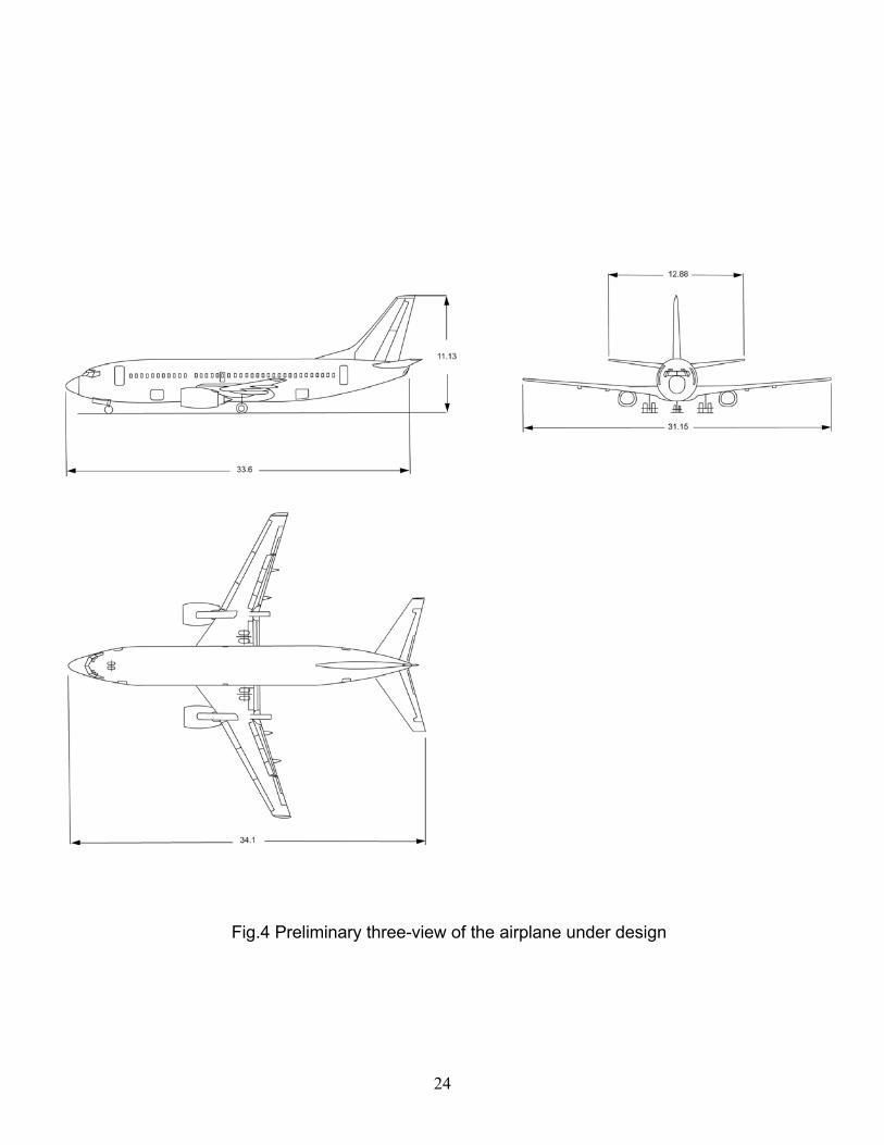
1.2.8 Overall height
Based on the dimensions of Boeing 737 - 300, 400 and 500, the overall height is
chosen as 11.13 m.
The preliminary three-view drawing of the airplane under design, is shown in Fig.4.

15
A B C D E F G H I Manufacturer
AIR-BUS
AIR-BUS
BOE-ING
BOE-ING
BOE-ING
BOE-ING
BOE-ING
BOE-ING
Type A319-
A320-
727- 737- 737- 737- 737- 737-
Model 100 200
200Adv
300 400 500 600 700
Initial service date
1995
1988
1970
1967
1967
1967
1998
1997
In service (ordered)
Africa 2(1) 27(6) 58 14(1) 7 17 (7) (2) Middle East/Asia/ Pacific
(4) 162 (47)
52 194 (19)
142 (5)
49(2) -
9(24)
Europe & CIS
48(82)
244 (105)
94 272 (12)
216(4) 145(1) 6(49) 21 (35)
North & South America
57 (264)
237 (146)
799
573 (11)
97(5)
165(1)
-
36 (146)
Total aircraft 107 (351)
670 (304)
1003 1053 (43)
462 (14)
376(4) 6(56) 66 (207)
Engine Manufacturer
CFMI
CFMI
P&W
CFMI
CFMI
CFMI
CFMI
CFMI
Model / Type
CFM 56-5A4
CFM 56-5A3
JTSD- 15A
CFM56-3-B1
CFM56-3B-2
CFM56-3-B1R
CFM56 -&B1B
CFM56 -JB20
No.of engines
2
2
3
2
2
2
2
2
Static thrust (kN)
99.7 111.2
71.2 89.0 97.9 82.3 82.0 89.0
Operation-al Items:
Accomodation
Max.seats (single class)
153
179
189
149
170
130
132
149
Two class seating
124
150
136
128
146
108
108
128
Table A – Data on 150 seater category airplanes (Contd…)
(Source http://www.bh.com/companions/034074152X/)

16
A B C D E F G H I Manufacturer
AIR-BUS
AIR-BUS
BOEI-NG
BOEI-NG
BOEI-NG
BOEI-NG
BOEI-NG
BOEI-NG
Type A319- A320- 727- 737- 737- 737- 737- 737- Model 100 200 200A
dv 300 400 500 600 700
No.abreast 6 6 6 6 6 6 6 6 Hold volume(m3)
27.00
38.76
43.10
30.20
38.90
23.30
23.30
30.2
Volume per Passenger
0.18
0.22
0.23
0.20
0.23
0.18
0.18
0.20
Mass (kg): Ramp 64400 73900 95238 56700 63050 52620 65310 69610 Max.take-off 64000 73500 95028 56470 62820 52390 65090 69400 Max.landing 61000 64500 72575 51710 54880 49900 54650 58060 Zero-fuel 57000 60500 63318 47630 51250 46490 51480 54650 Max.payload
17390 19190 18597 16030 17740 15530 9800 11610
Max.fuel payload
5360
13500
24366
8705
13366
5280
7831
10996
Design payload
11780
14250
12920
12160
13870
10260
10260
12160
Design fuelload
13020
17940
35944
12441
15580
11170
18390
19655
Operational Empty
39200
41310
46164
31869
33370
30960
36440
37585
Weight Ratios
Opsempty/ Max. T/O
0.613
0.562
0.486
0.564
0.531
0.591
0.560
0.542
Max. payload/ Max T/O
0.272
0.261
0.196
0.284
0.283
0.296
0.151
0.167
Max. fuel/ Max. T/O
0.295
0.256
0.255
0.281
0.253
0.303
0.316
0.296
Max.landing/ Max. T/O
0.953
0.878
0.764
0.916
0.874
0.952
0.840
0.837
Fuel (litres): Standard 23860 23860 30622 20105 20105 20105 26024 26024 Optional 40068 23170 23170 23170 Table A (Contd….)

17
A B C D E F G H I Manufacturer AIRBUS AIRBUS BOEING BOEING BOEING BOEING BOEING BOEING Type
A319-
A320-
727-
737-
737-
737-
737-
737-
Model 100 200 200Adv 300 400 500 600 700 DIMENSIONS Fuselage: Length(m) 33.84 37.57 41.51 32.30 35.30 29.90 29.88 32.18 Height(m) 4.14 4.14 3.76 3.73 3.73 3.73 3.73 3.73 Width(m) 3.95 3.95 3.76 3.73 3.73 3.73 3.73 3.73 Finess Ratio 8.57 9.51 7.00 7.40 7.40 7.40 7.40 7.40 Wing: Area(m2) 122.40 122.40 157.90 91.04 91.04 91.04 124.60 124.60 Span(m)
33.91
33.91
32.92
28.90
28.90
28.90
34.30
34.30
MAC(in) 4.29 4.29 5.46 3.73 3.73 3.73 4.17 4.17 Aspect Ratio 9.39 9.39 6.86 9.17 9.17 9.17 9.44 9.44 Taper Ratio 0.340 0.240 0.309 0.240 0.240 0.240 0.278 0.278 Average (t/c)%
11.00
12.89
12.89
12.89
¼ Chord Sweep(“)
25.00
25.00
32.00
25.00
25.00
25.00
25.00
25.00
High Lift Devices:
Trailing Edge flaps type
F1
F1
F3
S3
S3
S3
S2
S2
Flap Span/ Wing Span
0.780
0.780
0.740
0.720
0.720
0.720
0.599
0.599
Area (m2) 21.1 21.1 36.04 Leading edge Flap type
slats slats slats/ flaps
slats/ flaps
slats/ flaps
slats/ flaps
slats/ flaps
slats/ flaps
Area (m2) 12.64 12.64 Vertical Tail: Area (m2) 21.50 21.50 33.07 23.13 23.13 23.13 23.13 23.13 Height (m) 6.26 6.26 4.60 6.00 6.00 6.00 6.00 6.00 Aspect Ratio 1.82 1.82 0.64 1.56 1.56 1.56 1.56 1.56 Taper Ratio 0.303 0.303 0.780 0.310 0.310 0.310 0.310 0.310
Table A (Contd….)
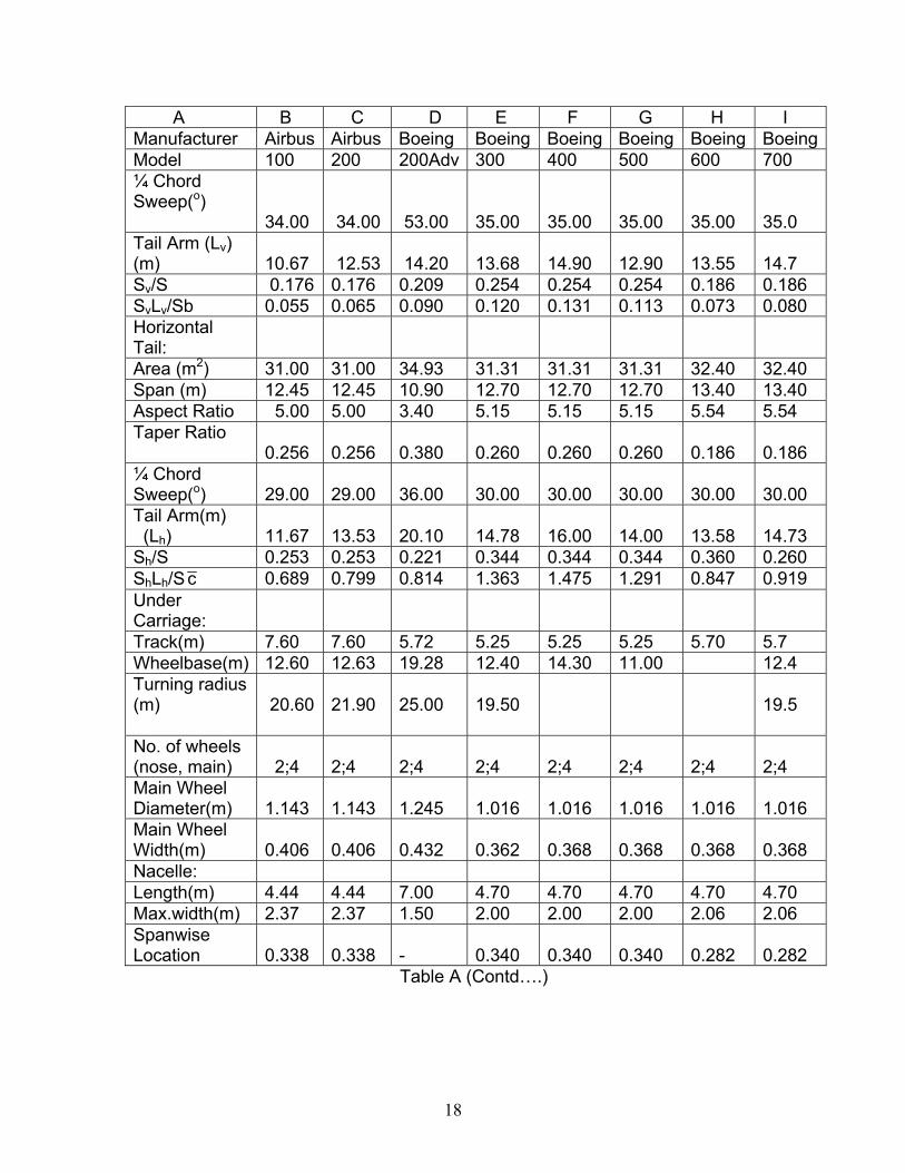
18
A B C D E F G H I Manufacturer Airbus Airbus Boeing Boeing Boeing Boeing Boeing BoeingModel 100 200 200Adv 300 400 500 600 700 ¼ Chord Sweep(o)
34.00
34.00
53.00
35.00
35.00
35.00
35.00
35.0
Tail Arm (Lv) (m)
10.67
12.53
14.20
13.68
14.90
12.90
13.55
14.7
Sv/S 0.176 0.176 0.209 0.254 0.254 0.254 0.186 0.186 SvLv/Sb 0.055 0.065 0.090 0.120 0.131 0.113 0.073 0.080 Horizontal Tail:
Area (m2) 31.00 31.00 34.93 31.31 31.31 31.31 32.40 32.40 Span (m) 12.45 12.45 10.90 12.70 12.70 12.70 13.40 13.40 Aspect Ratio 5.00 5.00 3.40 5.15 5.15 5.15 5.54 5.54 Taper Ratio
0.256 0.256
0.380
0.260
0.260
0.260
0.186
0.186
¼ Chord Sweep(o)
29.00
29.00
36.00
30.00
30.00
30.00
30.00
30.00
Tail Arm(m) (Lh)
11.67
13.53
20.10
14.78
16.00
14.00
13.58
14.73
Sh/S 0.253 0.253 0.221 0.344 0.344 0.344 0.360 0.260 ShLh/S c 0.689 0.799 0.814 1.363 1.475 1.291 0.847 0.919 Under Carriage:
Track(m) 7.60 7.60 5.72 5.25 5.25 5.25 5.70 5.7 Wheelbase(m) 12.60 12.63 19.28 12.40 14.30 11.00 12.4 Turning radius (m)
20.60
21.90
25.00
19.50
19.5
No. of wheels (nose, main)
2;4
2;4
2;4
2;4
2;4
2;4
2;4
2;4
Main Wheel Diameter(m)
1.143
1.143
1.245
1.016
1.016
1.016
1.016
1.016
Main Wheel Width(m)
0.406
0.406
0.432
0.362
0.368
0.368
0.368
0.368
Nacelle: Length(m) 4.44 4.44 7.00 4.70 4.70 4.70 4.70 4.70 Max.width(m) 2.37 2.37 1.50 2.00 2.00 2.00 2.06 2.06 Spanwise Location
0.338
0.338
-
0.340
0.340
0.340
0.282
0.282
Table A (Contd….)

19
Manufacturer AIR-BUS
AIR-BUS
BOE-ING
BOE-ING
BOE-ING
BOE-ING
BOE-ING
BOE-ING
Type A319- A320- 727- 737- 737- 737- 737- 737- Model 100 200 200Adv 300 400 500 600 700 PERFORMANCE
Loadings: Max.power load(kgf/kN)
320.96
330.49
444.89
317.25
320.84
318.29
396.89
389.89
Max wing load (kgf/m2)
522.88
600.49
601.82
620.28
690.03
575.46
522.39
556.98
Thrust/Weight Ratio
0.3176
0.3084
0.2291
0.3213
0.3177
0.3203
0.2568
0.2615
Take-off(m): ISA sea level 1750 2180 3033 1939 2222 1832 ISA +20oC SL 2080 2590 3658 2109 2475 2003 1878 2042 ISA 5000 ft 2360 2950 3962 2432 2316 ISA +20oC 5000ft
2870 4390 4176 2637 2649
Landing (m): ISA sea level 1350 1440 1494 1396 1582 1362 1268 1356 ISA +20oC SL 1350 1440 1494 1396 1582 1362 1268 1356 ISA 5000ft 1530 1645 1661 1576 1695 1533 ISA +20oC 5000 ft
1530
1645
1661
1576
1695
1533
Speeds (kt*/Mach):
V2 133 143 166 148 159 142 Vapp 131 134 137 133 138 130 Vno/Mno 381/
M 0.89 350/ M 0.82
390/ M 0.90
340/ M 0.82
340/ M 0.82
340/ M 0.82
392/ M 0.84
392/ M 0.84
Vne/Mne 350/ M 0.82
381/ M 0.89
M0.95
CLmax(T/O) 2.58 2.56 1.90 2.47 2.38 2.49 CLmax(Landing @MLM)
2.97 3.00 2.51 3.28 3.24 3.32
Table A (Contd….)
* 1 kt = 1.853 kmph

20
Manufacturer Airbus Airbus Boeing Boeing Boeing Boeing Boeing Boeing Type A319- A320 727- 737- 737- 737- 737- 737- Model 100 200 200Adv 300 400 500 600 700 Max.cruise: Speed (kt)* 487 487 530 491 492 492 Altitude (ft) 33000 28000 25000 26000 26000 26000 41000 41000 Fuel mass consumption (kg/h)
3160
3200
4536
3890
3307
3574
Long range Cruise:
Speed (kt) 446 448 467 429 430 429 450 452 Altitude (ft) 37000 37000 33000 35000 35000 35000 39000 39000 Fuel mass consumption (kg/h)
1980
2100
4309
2250
2377
2100
1932
2070
Range(nm*): Max payload 1355 637 2140 1578 1950 1360 Design range
1900
2700
2400
2850
2700
1700
3191
3197
Max fuel (+ payload)
4158
3672
3187
2830
3450
3229
3245
Ferry range Design Parameters:
W/SCLmax
(N/m2) 1726.69 1962.27 2356.82 1852.54 2090.56 1701.59
W/SCLtoST 2071.39 2423.85 3918.96 2196.64 2506.93 2024.27 Fuel/pax/ (kg)
0.0553
0.0443
0.1101
0.0341
0.0395
0.0608
0.0534
0.0480
Seats Range (seats nm)
235600
405000
326400
364800
394200
183600
344628
409216
1 kt = 1.853 kmph ; 1 nm = 1.853 km Table A – Data on 150 seater category airplanes (Concluded)
(Source http://www.bh.com/companions/034074152X/)

21
Fig.1 Three-view drawing of Boeing 737-300 Adapted from : http://www.the-blueprints.com
22
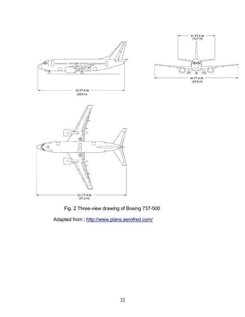
Fig. 2 Three-view drawing of Boeing 737-500 Adapted from : http://www.plans.aerofred.com/

23
Fig. 3 Three-view drawing of Boeing 737-700 Adapted from : http://www.the-blueprints.com
24
Fig.4 Preliminary three-view of the airplane under design

25
2 Revised weight estimation
In the previous section, an initial estimate for the aircraft parameters has
been carried out. In this section a revised weight is obtained by estimating fuel
weight and empty weight. According to Ref.4, chapter 3, the gross weight (Wg or
W0) is expressed as :
Wg = Wpay + Wcrew + Wf + We ; Wf = weight of fuel and We = empty weight (12a)
Dividing by Wg gives:
pay crew ef
g g g
W +W WW1 = + +
W W W
(12b)
To obtain revised estimate of Wg, (Wf / Wg) and (We / Wg ) are estimated in
sections 2.1 and 2.2.
Subsequently, pay crewg
ef
g g
W +WW =
WW1- +
W W
(12c)
2.1 Fuel fraction estimation
The fuel weight depends on the mission profile and the fuel required as reserve.
The mission profile for a civil jet transport involves:
Take off
Climb
Cruise
Loiter before landing
Descent
Landing
2.1.1 Warm up and take-off
The weight of the airplane at the start of take-off is W0 and the weight of the
airplane at the end of the take-off phase W1. The ratio (W1/W0) is estimated using
the guidelines given in Ref.4, chapter 3.
1
0
W=0.97
W

26
2.1.2 Climb
The weight of the airplane at the start of climb is W1 and the weight of the
airplane at the end of the climb phase is W2. The ratio ( 2W / 1W ) for this phase is
estimated following the guidelines given in Ref.4, chapter 3.
2
1
W=0.985
W
2.1.3 Cruise
The weight of the airplane at the start of cruise is W2 and the weight of the
airplane at the end of the cruise phase is W3. The ratio ( 3W 2/ W ) for the cruise
phase of flight is calculated using the following expression from Ref.4, chapter 3.
3
2 cruise cruise
W -RC= exp
W V (L / D)
; C = TSFC during cruise (13)
Gross still air range (GSAR) of the airplane is prescribed as 4000 km. Hence, the
Safe range during cruise GSAR 4000
= =26671.5 1.5
km
(L/D)max is taken as 18 from Fig. 3.6 of Ref.4. This value corresponds to an
average value for civil jet airplanes.
As prescribed in Ref.4, chapter 3,
(L/D)cruise = 0.866(L/D)max (14)
Hence, (L/D)cruise = 0.866 × 18 = 15.54
The allowances for (a) additional distance covered due to head wind during
cruise and (b) provision for diversion to another airport in the event of landing
being refused at the destination, are obtained as follows.
Head wind is taken as 15 m/s.
The cruise is at M = 0.8 at 11 km altitude. The speed of sound at 11 km altitude
is 295.2 m/s. Hence, Vcruise is 236 m/s or 849.6 kmph
The time to cover the cruise range of 2667 km at Vcr of 849.6 km/hr is :
2667Time = = 3.13 hours
849.6

27
Therefore, with a head wind of 15 m/s or 54 km/hr the additional distance needed
to be accounted for is :
Additional distance = 54 × 3.13 = 169 km
The allowance for diversion to another airport is taken as 400 km.
The total extra distance that is to be accounted for : 169 + 400 = 569 km.
The total distance during the cruise (R) = 2667 + 569 = 3236 km.
Following guidelines from Ref.4 chapter 3, TSFC during cruise is taken as
0.6 hr-1.
Substituting the various values in Eq.(13) yields,
3
2
W -3236×0.6= exp = 0.863
W 849.6×15.59
2.1.4 Loiter Sometimes the permission to land at the destination is not accorded immediately
and the airplane goes around in circular path above the airport. This phase of
flight is called loiter. The weight of the airplane at the end of loiter is 4W . The
ratio ( 4W 3/ W ) is calculated using the following expression from Ref.4, chapter 3.
4
3
W -E×TSFC= exp
W (L / D)
(15)
During Loiter, the airplane usually flies at a speed corresponding to (L/D)max .
Hence, that value is used in Eq.(15). The loiter time (E) is taken as 30 minutes
(0.5 hr). TSFC is taken as 0.6 hr-1.
Hence,
4
3
W -0.5 × 0.6= exp = 0.983
W 18
2.1.5 Landing
The weight of the airplane at the start of landing is W4 and the weight of the
airplane at the end of the landing is W5. Following the guidelines specified by
Ref.4, chapter 3, the ratio W5 4/ W is taken as :

28
5
4
W= 0.995
W
Finally,
5 5
g 0
W W= =0.97 × 0.985 × 0.863 × 0.983 × 0.995 = 0.806
W W
Allowing for a reserve fuel of 6%, the fuel fraction for the flight, or (Wf/ Wg ) is
given by :
5f
g 0
WW= = 1.06 1- = 0.205
W W
ζ
2.2 Empty weight fraction
The ratio (We/ Wg ) is called empty weight fraction. To determine this fraction, the
method given in Ref.4, chapter 3, is used. The relationship between We/Wg and
Wg for a jet transport is as follows.
-0.06eg
g
W= 1.02(2.202W )
W ; where, Wg is in kgf (16)
From subsection 1.2.1, (Wpay + Wcrew) is 17270 kgf.
Substituting in Eq.(12a) :
pay crew
g -0.06gf g e g
W W 17270W = =
1 - 0.205 - 1.202(2.202W )1- W / W - W / W
(16a)
Both the sides of Eq.(16a) involve Wg. The solution of this equation is obtained
by an iterative procedure. A guessed value of gross weight, (Wg (guess)), is
substituted on the right hand side of Eq.(16a) and value of Wg is obtained. If the
obtained value and the guest value are different, a new guest value is used. The
steps are repeated till the guest value and the obtained value are same. The
procedure is presented in Table 3.

29
Wg (guess) We/Wg(from eq.(16)) Wg(from eq.(16a))
60000 0.50274 59090
59090 0.50320 59184
59184 0.50315 59174
59174 0.50316 59175
59175 0.50316 59175
Table 3: Iterative procedure for Wg
Hence, the gross weight Wg is obtained as:
Wg = 59, 175 kgf
The important weight ratios are:
e
g
W= 0.503
W; f
g
W= 0.205
W; pay crew
g
W +W= 0.292
W
3 Wing loading and thrust loading
The thrust-to-weight ratio (T/W) and the wing loading(W/S) are the two
most important parameters affecting aircraft performance. Optimization of
these parameters forms a major part of the design activities conducted after
initial weight estimation. For example, if the wing loading used for the initial
layout is low, then the wing area would be large and there would be enough
space for the landing gear and fuel tanks. However, it results in a heavier wing.
Wing loading and thrust-to-weight ratio are interconnected for a number
of critical performance items, such as take-off distance, maximum speed, climb,
range etc. These two are often the design drivers. A requirement for short
take-off can be met by using a large wing (low W/S) with a relatively low T/W. On
the other hand, the same take-off distance could be met with a high W/S along
with a higher T/W.
In this section, different criteria are used to optimize the wing loading and thrust
loading.
Wing loading affects stalling speed, climb rate, take-off and landing distances,
minimum fuel required for range and turn performance.

30
Similarly, a higher thrust loading would result in more cost which is undesirable.
However, it would also lead to enhanced climb performance.
Hence, a trade-off is needed while choosing W/S and T/W. Optimization
of W/S and T/W based on various considerations is carried out in the following
subsections.
3.1 Landing distance consideration
To decide the wing loading from landing distance consideration the landing field
length needs to be specified. Based on data collection of similar airplanes in
Table A, the landing field length is chosen to be 1425 m.
sland = 1425 m
Next, the CLmax of the airplane is chosen. The Maximum lift coefficient
depends upon the wing geometry, airfoil shape, flap span and geometry, leading
edge slot or slat geometry, Reynolds number, surface texture and interference
from other parts of the airplane such as the fuselage, nacelles or pylons.
Reference 4, chapter 5 provides a chart for CLmax as a function of c/4Λ for
different types of high lift devices. For the airplane under design, it is decided to
use Fowler flap and slat as the high lift devices. This gives CLmax of 2.5 for a
oc/4Λ = 25 .
To calculate W/S based on landing considerations, the following formula is used.
2s Lmax
W 1= ρV C
S 2 (17)
The stalling speed Vs is estimated in the following manner.
(a) sland is prescribed as = 1425 m = 4675.2 feet
(b) According to Ref.4, chapter 3, the approach speed (Va) in knots is related to
the landing distance(sland) in feet as,
Valands (in feet)
(inknots) =0.3
(c) Va = 1.3 Vs
In the present case

31
(Va) (in knots) = 4675.2
= 124.84 kts = 64.25 m/s1.3
Hence, -1s
64.25V = = 49.4 ms
1.3 (18)
Now, using this value for Vs in Eq.(17),
-2
land
W= 3743 Nm
S
From Ref.4, chapter 3, for this type of airplane, Wland = 0.85 WTO. Hence, W/S based on WTO is :
-2
TO Land
W 1 W= = 4403 Nm
S 0.85 S
Allowing 10 % variation in Vs , gives the following range of wing loadings for
which the landing performance is near optimum:
23639 < p < 5328 N/ m 3.2 Maximum speed (Vmax) consideration The optimization of wing loading from consideration of Vmax is carried out through
the following steps.
(I) For jet transport airplanes, Vmax is sometimes decided based on the value of
maximum Mach number (Mmax). In turn Mmax is taken as :
Mmax = Mcruise + 0.04 Hence, Mmax = 0.80 + 0.04 = 0.84 and Vmax = 0.84 x 295.2 = 248 m/s (II) The estimation of drag polar and its alternate representation are carried out
as follows. It may be noted that the procedure given below is slightly different
from that given in subsection 4.4.1 of Ref.5.
The drag polar is expressed as :
2D DO LC = C + KC (19)

32
where,
1K =
πAe; e = Oswald efficiency factor (20)
Following Ref.4, chapter 2, DOC is given as :
wetDO f e
SC = C ×
S , (21)
where, Cfe = equivalent skin friction drag coefficient ; Swet = Wetted area of the
airplane.
From Fig 2.5 of Ref.4, Swet/S = 6.33.
The estimation of K is carried out next and then the value of DOC is deduced
using the earlier assumption that (L/D)max is 18.
Estimation of K: The value of Oswald efficiency factor (e) is estimated from Ref.6, chapter 2 as :
wing fuse
1 1 1= + + 0.05
e e e (22)
From Ref.12, chapter 1,
ewing = 0.84 for an unswept wing of A = 9.3 and λ = 0.24.
From Ref.9, chapter 7, ewing for a swept wing is :
wing wingΛ Λ=0e = e cos Λ - 5
Hence, in the present case, winge = 0.84 cos (25 -5) = 0.7893 (23)
From Ref.6, chapter 2 fuse
1= 0.1
e
Finally, 1 1
= +0.1+0.005e 0.7893
or e = 0.707
1K = = 0.0482
π×9.3×0.707

33
To get DOC , it is recalled that (L/D)max = 18 was assumed in subsection 2.1.3.
Further,
max
D0
1(L / D) =
2 C K (24)
Hence,
D0 2 2max
1 1C = = =0.0161
4K(L / D) 4×0.0482×18
Using this value of D0C in Eq.21, gives Cfe as :
f e
0.0161C = = 0.00254
6.33 (25)
Hence, the drag polar is :
2D LC = 0.0161+0.0482 C (25a)
Alternate representation of drag polar :
To obtain the optimum W/S based on maximum speed, the method given in
Ref.7, is followed. It is also described in section 4.4 of Ref.5. The drag polar is
expressed as :
2D 1 2 3C = F +F p+F p (26)
where,
ht vt wet1 fe fe t
w
S S SF = C 1+ + = C K
S S S
(27)
D0 12
(C -F )F =
W / S (28)
3 2
KF =
q (29)
Two values of F1, F2 and F3 are obtained as follows. From section 1.2 and subsections 1.2.1 to 1.2.7:
htS= 0.31
S
vtS= 0.21
S

34
Hence,
ht vtt
S SK = 1 + + = 1 + 0.31 + 0.21 = 1.52
S S
wet(exposed)Do feW
W
SC = C
S
(30)
To calculate (Swet(exposed)/S), the dimensions of the exposed wing are obtained as
follows. From subsection 1.2.2, the parameters of the equivalent trapezoidal wing
(ETW)are :
S = 107.02 m2
λ = 0.24 A = 9.3 b = 31.55 m cr = 5.47 m ct = 1.31 m o
c/4Λ =25
Hence, for ETW, the chord distribution is givenby :
r tr
c -cc(y) = c -
b / 2= 5.47 − 0.264y
Taking fuselage diameter of 3.79 m, the chord at y = 1.895 m is the root chord of
the exposed wing, (cr(exposed)) i.e.
cr(exposed) = = 5.47 − 0.264 x 1.895 = 4.97 m
Semi-span of the exposed wing is 31.55 3.79
= - = 13.89 m2 2
Hence, 2exposedwing
1S = (4.97+1.31)×13.89×2 = 87.23 m
2
The wetted area of the exposed wing ( wet(exposed wing)S ) is approximated as :
exposed wing exposedwing avgwetS = 2S 1+1.2(t / c) (31)
Assuming (t/c)avg of 12.5%, 2
wet(exposed wing)S = 2 87.23 1+1.2 (0.125) = 200.63 m
Hence,
D0 W
200.63(C ) = 0.0025× = 0.004687
107.02
F1 = 1.52 × 0.004687 = 0.007124

35
-6 2Do 12
C -F 0.0161 - 0.007124F = = = 1.632×10 m / N
W / S 5500
The above drag polar will not be valid at M greater than the Mcruise.
Hence, the drag polar (values of CDO and K) at Mmax needs to be estimated .
The drag divergence Mach number (MD) for the aircraft is fixed at M = 0.82
which is 0.02 greater than Mcruise. This would ensure that there is no wave
drag at Mcruise of 0.80. To estimate the increase in CDO from M = 0.80 to
M = 0.84, a reasonable assumption is that the slope of the CDO vs M curve
remains constant in the region between M = 0.82 and M = 0.84.
The value of this slope is 0.1 at M = 0.82. Hence, the increase in CDO is
estimated as 0.02 × 0.1 = 0.002.
From the data on B 787 available in website [Ref.2], it is observed that the
variation in K is not significant in the range M = 0.82 to 0.84. Hence, the value
of K is retained as in subcritical flow. However, better estimates are used in
performance calculations presented later (subsection 9.3.2).
Consequently, the drag polar that is valid at Mmax is estimated as :
2D LC = 0.0181 + 0.0482C (32)
The change in the CDO is largely due to change in the zero lift drag of the
wing, horizontal tail and vertical tail. This means that the change in CDO
affects the value of F1 alone.
Hence, at Mmax , F1 = 0.009124
The value of F3 depends on the dynamic pressure at Vmax.
max max cruiseV = M × speedof soundath = 0.84×295.2 = 248 m / s
2 2max max
1q = ρV = 0.5×0.364×248 = 11200.95
2
-10 4 23 2
0.0482F = = 3.84×10 m / N
11200.95
The optimum value of W/S, from Vmax consideration, is the wing loading (p)
which minimises thrust required for Vmax . The relation between the thrust
required for Vmax and p is:

36
1Vmax max 2 3
Ft = q +F +F p
p
; Vmaxt = (thrust required for Vmax ) / W (33)
Differentiating Eq.(33) and equating to zero gives the optimum wing loading
(poptimum) i.e.
vmax 1max 32
t F= q +F = 0
p p
Or 1optimum
3
Fp =
F
Hence, in the present case : 2optimum -10
0.009124p = = 4873.31N / m
3.84×10
The value of Vmaxt with p = optimump is found from Eq.(33) as :
Vmaxt = -6 -100.00912411200.95 +1.632×10 +3.84×10 ×4873.31
4873.31
= 0.06022 (33a)
If the value of Vmaxt can be permitted to be 5 % higher than the minimum in
Eq.(33a), i.e. 0.0632, Eq. (33) gives two values of p viz.
p1 = 3344 Nm-2
p2 = 7101 Nm-2
Thus, any value of p between 3344 and 7101 would be acceptable from Vmax
considerations with a maximum of 5% deviation from the optimum.
3.3 (R/C)max consideration
The value for (R/C)max at sea level is chosen as 700 m/min (11.67 m/s)
which is typical for passenger airplanes.The thrust required for climb at chosen
flight speed(V ) is related to (R/C) in the following manner(section 4.6 of
Ref.5).
R/c D
R / C qt = + C
V p ; R/ct = (Thrust required for climb) / W (34)
However, CD can be represented as :
CD = F1 + F2 p + F3p2
(35)

37
20
1q = ρ σV
2 (36)
Hence,
2
2R/c 0 1 2 3
R / C 1 Vt = + ρ σ F +F p+F p
V 2 p (37)
The flight speed for optimum climb performance is generally not high and value
of F1 corresponding to its value for M < Mcruise is appropriate. However, F3 is a
function of the dynamic pressure and depends on chosen flight velocity.
The aim here is to find the minimum sea level static thrust ( SR/Ct ) for various
values of V and then choose the minimum amongst the minima. For a chosen
V , differentiating Eq.(37) with p and equating to 0 gives the optimum wing
loading as
1opt
3
Fp =
F (37a)
Choosing different values of V, the values of popt and R/Ct are obtained using
Eqs.(37a) and (37). These values are presented in first 3 columns of Table 4.
However, the aim of the optimization is to obtain an engine with minimum sea
level static thrust (Ts). Since, thrust output varies with flight speed the values of
R/Ct need to be converted to SR/Ct . Where, SR/Ct is (Ts / W). The value of Ts is
chosen for the climb setting. The values of T at different velocities are obtained
from Ref.8, chapter 9 for an engine with bypass ratio of 6.5. The value of
R/Ct multiplied by (Ts/T) gives SR/Ct . The values of SR/Ct are also given in Table 4.
It is observed that R/ct has a minimum of 0.2469 at p = 4615. However, the values
of sR/ct are only slightly different from the minimum for values of V from 120 to
170 m/s. Hence, for wingloading (p) between 3391 to 6805 N/ m2 the thrust
loading would be close to the optimum.

38
V
(m/s)
popt R/ct sR/ct
80 1507 0.1893 0.2868
100 2355 0.1637 0.2641
120 3391 0.1487 0.2507
140 4615 0.14 0.2469
150 5298 0.1373 0.2483
160 6028 0.1356 0.2510
170 6805 0.1346 0.2554
180 7629 0.1343 0.2617
190 8500 0.1345 0.2691
200 9419 0.1354 0.2780
Table 4: Variation of sR/ct with different values of V
3.4 Minimum fuel for range (Wfmin) consideration
In cruise, the weight of the fuel (Wf) used is to cover the range (R) is related to
the wing loading (p) as given below (section 4.7 of Ref.5).
0 1f 2 3
ρ FRW = TSFC σq +F +F p
3.6 2 p
(38)
The values of F1, F2 and F3 corresponding to cruise conditions are as follows.
F1 = 0.007124
F2 = 1.632 × 10⁻⁶
Vcruise = Mcruise × 295.2 = 0.8 × 295.2 = 236.3 m/s
qcruise = 0.5 × ρ × 2cruiseV = 0.5 × 0.364 × 236.32
= 10159.59 N/m2
Hence, 2
-10 4 23
0.0482F = =4.67 × 10 m / N
10159.59
Differentiating Eq.(38) by p and equating to 0 gives the optimum wing loading
from range consideration as :

39
1optimum R
3
Fp =
F (39)
In this case, 2optimum -10R
0.007124p = = 3905.84 N / m
4.67×10
Using this value of p, in Eq.(38) along with R = 4000 km and
TSFC = 0.6 hr−1, yields :
fminW = 0.1514
Allowing an excess fuel of 5 % i.e. f minW = 0.1590 and using Eq.(38) gives
two values p1 and p2 as :
p1 = 2676 N/m2
p2 = 5700 N/m2
Thus, a value of p within p1 and p2 would be acceptable from the point of view
of minimizing fW .
3.5 Absolute ceiling consideration
At absolute ceiling (Hmax), the flight is possible at only one speed. Observing the
trend of Hmax as hcruise + 0.6 km the absolute ceiling Hmax is chosen as
11.6 km. To find the Hmaxt , the following two equations are solved (section
4.5 of Ref.5).
h 1 2t = 4K(F +F p) (40)
1h hmax 2
Ft =2q +F
p
(41)
The values of F1 and F2 corresponding to this case are :
F1 = 0.007124
F2 = 1.632 × 10⁻⁶
In the absence of a prescribed velocity at Hmax, the velocity corresponding
to flight at (L/D)max is assumed to calculate Hmaxq . The value of CL corresponding
to (L/D) max is given by :

40
DoL
C 0.0161C = = = 0.577
K 0.048 (42)
HmaxL
(W / S) 5500q = = = 9532.06
C 0.577
The solution for popt is obtained by solving Eqs.(40) and (41).
popt = 5500 Nm-2 as it should be.
Hmaxt corresponding to poptimum is :
Hmaxt = 0.05581
Allowing a 5 % variation in Hmaxt , gives the following two values.
Hmax1t = 0.05302
Hmax2t = 0.05860
The solutions to Eq.(40) with the new Hmaxt values are:
p1p1 = 4567 Nm-2
p2 = 6547 Nm-2
Similarly, using in Eq.(41), the two values are :
1p = 4942 Nm-2
2p = 6201 Nm-2
From the above four values, the lower and upper bounds for values of p from the
ceiling considerations are
1p = 4942 Nm-2
2p = 6201 Nm-2
Hence, for p between 4942 and 6201 N/m2 would be acceptable from
consideration of ceiling.
3.6 Choice of optimum wing loading
The range of wing loading which give near optimum results in various cases
discussed above are tabulated in Table 5.

41
Performance criteria Allowable range of W/S in (Nm-2)
sland 3639 - 5328
Vmax 3344 - 7101
(R/C)max 3391 - 6805
fW 2676 - 5700
hmax 4942 - 6201
Table 5: Allowable range of W/S in various cases
From the above table, it is observed that the range of wing loading in which all
the criteria are satisfied is 4942 to 5328 N/m2
3.7 Consideration of wing weight (Ww)
The weight of the wing depends on its area. According to Ref.4, chapter
15, for passenger airplanes, the weight of the wing is proportional to S0.6499.
Thus, a wing with lower area will be lighter and for wing area to be lower, the
W/S should be higher. However, for a passenger the consideration of fuel
required for range is also an important consideration. From section 3.4 it is noted
that the wing loading should be 3906 for fW to be minimum. At the same time
with a wing loading of 5700 N / m2, the value of fW is only 5 % higher than fminW
Hence, the advantage of choosing a wing loading higher than that indicated by
fminW requirement, is examined.
It may be pointed out that the weight of wing structure is about 12% of Wg.
The optimum W/S from range consideration is 3906 N/m2 whereas with
a 5% increase in Wf , the wing loading could go up to 5700 N/m2. If the
wing loading of 5700 N/m2 is chosen, instead of 3906 N/m2, the weight of
the wing would decrease by a factor of :
0.6493906
= 0.7825700

42
With weight of the wing as 12 % of Wg, the saving in the wing weight when higher
wing loading is chosen is :
12 x (1-0.782) = 2.6 %.
However, this higher wing loading results in an increase in fuel by 5 % of Wf. In
the present case, Wf is around 20% and hence a 5% in Wf means an increase in
the weight by 0.05 × 0.2 = 1%.
Thus, by increasing W/S from 3906 to 5700 N/m2, the saving in Wg
would be 2.6 - 1 = 1.6%. Thus, it is advantageous to have higher wing loading
W/S.
3.8 Final choice of W/S
It is observed from Table 5 that a wide range of wing loading is permissible which
still satisfies various requirements with permissible deviations from the optimum.
To arrive at the final choice, the take-off requirement is considered. The highest
wing loading which would permit take-off within permissible distance without
excessive (T/W) requirement is the criteria. From data collection,
the balanced field length for take-off is assumed to be 2150 m. From Fig.5.4
of Ref.4, the take-off parameter {(W/S)/ LTOC (T/W)} for this field length is 180.
With (W/S) in lb/ft2. The take-off is considered at sea level or = 1. The value of
LTOC is 0.8 x CLmax = 0.8 × 2.5 = 2. Generally the airplanes in this category have
(T/W) of 0.3. Substituting these values gives,
finalp = 108.2 lb/ft2 = 5195 Nm-2
It is reassuring that this value of p lies within the permissible values
summarized in Table 5.
3.9 Thrust requirements
After selecting the W/S for the aircraft, the thrust needed for various design
requirements is obtained. These requirements decide the choice of engine.
3.9.1 Requirement for Vmax
The chosen value of p i.e. 5195 Nm-2 is substituted in the following equation :

43
1Vmax max 2 3
Ft = q +F +F p
p
(43)
= 11200.95 -6 -100.009124+1.632×10 +3.84×10 ×5195
5195
= 0.0602 (44)
Referring to engine charts in Ref.8, chapter 9, for a turbo fan engine with bypass
ratio of 6.5, the thrust loading based on sea level static thrust is :
T 0.0602= = 0.334
W 0.18 (45)
In the present case, this would mean a thrust requirement of
Treq = 0.334 x 59175 x 9.81 = 193.9 kN
3.9.2 Requirements for (R/C)max
The following equation is used
22
R/c 0 1 2 3
R / C 1 Vt = + ρ σ (F + F p + F p )
V 2 p (46)
Substituting appropriate values, yields :
R/C
T= 0.252
W
(47)
In the present case, this implies a thrust requirement of 146.3 kN
3.9.3 Take-off thrust requirements
The value of (T/W) for take-off has been taken as 0.3.This implies a thrust
requirement of 0.3 x 59175 x 9.81 = 174.2 kN
3.10 Engine choice
From the previous section, it is observed that the maximum thrust requirements
occurs from Vmax consideration i.e. Tmax = 193.9 kN
As a twin engine configuration has been adopted, the above requirement implies
thrust per engine of 96.95 kN/engine.

44
An engine which supplies this thrust and has a TSFC of 0.6 hr−1 and bypass ratio
of around 6.5 is needed. Some of the engines which perform close to these
requirements are taken from Ref.8, chapter 9 and website 1.
Finally, CFM56-2B model of turbofan with a sea level static
thrust of 97.9 kN is chosen.
3.11 Engine characteristics
For calculation of the performance of the airplane, the variations of thrust and
TSFC with speed and altitude are required. Reference 8, chapter 9 has given
non-dimensional charts for turbofan engines with different bypass ratios.
Choosing the charts for bypass ratio = 6.5 and sea level static thrust of 97.9kN,
the engine curves are calculated and presented in Figs.5 and 6.
Fig. 5 Variations of thrust with Mach number at different altitudes
with cruise setting of engine.

45
Fig. 6 Variations of thrust with Mach number (a) at sea level with take-off setting and (b) at various altitudes with climb setting of engine 4 Wing Design
4.1 Introduction
The weight and the wing loading of the airplane have been discussed in sections
2 and 3 as 59175 kgf (579915 N) and 5195 N/m2 . These give wing area
as 111.63 m2 . The wing design involves choosing the following parameters.
1. Airfoil selection
2. Aspect ratio
3. Sweep
4. Taper ratio
5. Twist
6. Incidence
7. Dihedral
8. Vertical location
In the following subsections, the factors affecting the choice of these parameters

46
are mentioned and then the choices are effected.
4.2 Airfoil Selection
The airfoil shape influences CLmax , CDmin, CLopt , Cmac and stall pattern.
These in turn influence stalling speed, fuel consumption during cruise, turning
performance and weight of the airplane.
For high subsonic airplanes, the drag divergence Mach number(MD) is
an important consideration. It may be recalled that (MD) is the Mach
number at which the increase in the drag coefficient is 0.002 above the value
at low subsonic Mach numbers. A supercritical airfoil is specially designed to
increase MD. NASA has carried out tests on several supercritical airfoils and
recommends the use of NASA-SC(2) series airfoil with appropriate thickness
ratio and camber.
4.2.1 Design lift coefficient
The CLopt of an airfoil is the lift coefficient at which the drag coefficient is
minimum. For passanger airplanes, the airfoil is chosen in such a way that CLopt
equals LcruiseC .
Lcruisecruise
(W / S)C =
q (48)
Using the value of (W/S) = 5195 Nm-2 and q corresponding to
M = 0.8 at 11 km altitude, gives :
CLcruise = 0.512 (49)
CLopt is taken as 0.5 for choosing airfoil thickness ratio and wing sweep.
4.2.2 Airfoil thickness ratio and wing sweep
Airfoil thickness ratio (t/c) has a direct influence on drag, maximum lift, stall
characteristics, structural weight and critical Mach number. A higher t/c implies
a lower critical Mach number but also a lower wing weight. Thus, an optimum t/c
for the airfoil needs to be chosen.
CLopt = 0.5 has been chosen and the cruise Mach number is 0.8. In order
47
to ensure that the drag divergence Mach number is greater than Mcruise,
MD is chosen as 0.82. This is based on the consideration that there should
be no increase in drag at Mcruise . It may be recalled that DwaveΔC is 0.002 at MD
and the slope of the CD Vs M curve around MD is 0.1.
Reference 3 gives experimental results for several super-critical airfoils with
different values of (t/c) and CLopt . Curves for CLopt = 0.4, 0.7, 1.0 are available in
the aforesaid report.The curve corresponding to CLopt = 0.5 is obtained by
interpolation.
The MD for the wing is estimated in the following manner.
MD = (MD)airfoil + MA + ΛM (50)
where, MA and ΛΔM are corrections for influences of the aspect ratio
and the sweep.
The change in MD with A is almost zero for A > 8. Since, A = 9.3, has been
chosen the second term in the above equation will not contribute to
MD. Further, from Ref.[9], chapter 15, the change in MD due to sweep
is given as :
DΛ
DΛ=0
1 - MΛ1 - =
90 1 - M (51)
The supercritical airfoil with (t/c) = 14% has MD = 0.74 at CLopt of 0.5. Using this in
Eq.(51) gives which would give DΛM of 0.82 i.e.
Λ 1-0.82
1 - =90 1-0.74
oOr Λ = 27.7
The average thickness has been chosen as 14 %. However, to reduce the
structural weight, the (t/c) at wing root is increased and the (t/c) at wing tip is
decreased, Considering the features for Airbus A310 and Boeing B 767 which
have Mcruise = 0.8 and similar values of 1/4Λ , it is decided that the variation of (t/c)
along the span be such that (t/c) is 15.2% at root, 11.8% at spanwise
48
location of the thickness break and 10.3% at the tip. Thickness break location is
the spanwise location upto which the trailing edge is straight. From the data
collection this location is at 34% of semi-span.
4.3 Other parameters
4.3.1 Aspect ratio
The aspect ratio affects LαC , DiC and wing weight. The value of LαC decreases
as A decreases. For example, in the case of an elliptic wing,
Lα lα airfoil
AC = C
A +2 (52)
The induced drag coefficient can be expressed as
2L
Di
CC = (1+δ)
πA (53)
where, depends on A, λ and . A high value of A increases the span of the
wing which in turn requires more hanger space. A higher aspect ratio would also
result in poor riding quality in turbulent weather. All these factors need
careful optimization. However, at the present stage of design, A = 9.3 is chosen
based on trends indicated by data collection.
Correspondingly, the wing span would be
b = AS = 9.3×111.63 = 32.22 m
4.3.2 Taper ratio
Wing taper ratio is defined as the ratio between the tip chord and the root chord.
Taper ratio affects :
Induced drag
Weight of wing and
Tip stalling
Induced drag is low for taper ratios between 0.3 - 0.5. Lower the taper ratio,
lower is the weight. A swept wing also has higher structural weight than
an unswept wing. Since, the present airplane has a swept wing, a taper ratio of

49
0.24 has been chosen based on the trends of current swept wing airplanes.
4.3.3 Root and tip chords
Root chord and tip chord of the equivalent trapezoidal wing can now be
evaluated.
r
2S 2×111.63c = = 5.59 m
b(1+λ) 32.22 1+0.24
t rc = c λ = 5.59×0.24 = 1.34 m
Mean aerodynamic chord (mac) = 2
r
2 (1 + λ + λ )c = c = 3.9 m
3 (1+λ)
The location of the quarter chord of the mac from leading edge of the
root chord is calculated as 4.76 m.
4.3.4 Dihedral
The dihedral is the angle of the wing with respect to the horizontal plane
when seen in the front view. Dihedral of the wing affects the lateral stability of the
airplane. Since, there is no simple technique for arriving at the dihedral angle
that takes all the considerations into effect, the dihedral angle is chosen based
on data collected (Table A). Hence, a value of oΓ = 5 is chosen.
4.3.5 Wing twist
A linear twist of 3 is chosen tentatively.
4.4 Cranked wing design
An observation of the design of current high subsonic airplanes, indicates that
the trailing edge is straight for a part of the span, in the inboard region. This
results in a larger chord in the inboard section as compared to a normal swept
wing which is trapezoidal in shape. A larger chord in the inboard region has
following advantages.
1. More space for fuel and landing gear.

50
2.The lift distribution is changed such that more lift is produced in the
inboard region of wing, which reduces the bending moment at the root.
This type of design is called a wing with cranked trailing edge. The value
of the span upto which the trailing edge is straight has to be obtained by
optimization considering drag and weight of wing. However, at the present stage
of design, based on the current trends, the trailing edge is made unswept till 35%
of the semi span in the present case, the semi-span of the wing portion with
unswept trailing edge is:
0.35 × (32.22/2) = 5.64 m
Fig. 7 Plan forms of ETW and cranked wing The cranked wing and the equivalent trapezoidal wing (ETW) are shown in Fig.7.
The planform of the cranked wing is obtained as follows.
(i) The area of the cranked wing = area of ETW = 111.63 m2
(ii) The span of the cranked wing = span of ETW = 32.22 m
(iii) Tip chord of the cranked wing (cte) = tip chord of ETW (ctc) = 1.34 m
(iv) Leading edge sweep of cranked wing = leading edge sweep of ETW = 30.58o
(v) Rootchord of ETW = cre = 5.59 m. The root chord of the cranked wing is

51
obtained in the next two steps.
(vi) As mentioned above, the straight portion with unswept trailing edge of the
cranked wing extends upto 5.64 m on either side of root chord. Because of this
choice, the leading edge of the chord at a spanwise location (y) of 5.64 m is:
5.64 x tan 30.58 = 3.33 m behind the leading edge of the root chord.
(vii) Let crc be the root chord of the cranked wing. Considering the shape of the
cranked wing in Fig.7 and noting that the area of the cranked wing is 111.63 m2,
gives the following equation for crc.
rc rc rcc +c -3.33 c -3.33+1.342 ×5.64+ × 16.11-5.64 = 111.63
2 2
Or crc = 6.954 m.
4.5 Wing incidence(iw)
The wing incidence is the angle between wing reference chord and
fuselage reference line. Wing incidence is chosen to minimize the drag at
some operating conditions,usually cruise.The wing incidence is chosen such
that when the wing is at the correct angle of attack for the selected design
condition, the fuselage is at the angle of attack for minimum drag(usually at
zero angle of attack). The wing incidence is finally set using wind
tunnel data. However, an initial estimate, of iw, for preliminary design purpose,
is obtained as follows.
Lcruise Lα w 0LC = C i - α (54)
In the present case,
LcruiseC = 0.512
LαC is calculated using the following formula in Ref.4, chapter 12,
exposedLα 22 2
refmax2 2
S2πAC = (F)
Stan ΛA β2+ 4+ (1+ )
η β
(55)
where,
2 2β = 1 - M

52
η = 1
2
dF = 1.07 1+
b
exposedS = area of exposed wing
maxΛ = sweep angle of the maximum thickness line of airfoil
Substituting various values, gives
-1LαC = 6.276 rad = 0.1095 deg-1
The zero lift angle 0Lα for the airfoil was calculated using camber line of the
supercritical airfoil with 14% thickness ratio. The value is o-5.8 . Substituting the
values yields a value of iw which is negative. This can be attributed to the fact that
the value of LαC as estimated above is high. It may be pointed out that in
Appendix ‘C’ of Ref.14, the stability derivatives of Boeing 747 are evaluated.
There also the calculated value of LαC at M = 0.8 is higher than the experimental
value. This is because the estimated value is for a rigid wing. The actual wing is
flexible and the theoretical increase in LαC due to Mach number, is not realizied.
owi = 1 is chosen. This value is recommended in Ref.4, chapter 4.
4.6 Vertical location of wing
The wing vertical location for the airplane under design is chosen as low wing
configuration. This is typical for similar airplanes.
4.7 Areas of flaps and ailerons
These areas are chosen based on the data on similar airplanes.
1.Trailing edge : Fowler flaps.
2.Leading edge : full span slats.
flapS= 0.17
S, slatS
= 0.1S
, flapspan
= 0.74wingspan

53
5 Fuselage and tail layout
5.1 Introduction
The fuselage layout is important in the design process as the length of the
airplane depends on this.The length and diameter of the fuselage are related
to the seating arrangement.
The Fuselage of a passenger airplane can be divided into four basic sections viz.
nose, cockpit, payload compartment and tail fuselage. In this section, the
fuselage design is carried out by choosing the parameters of these sections.
5.2 Initial estimate of fuselage length
Observing the values of (lf /b) for similar airplanes, a value of 1.05 is chosen.
Using b = 32.22 m as obtained from wing design, the fuselage length is :
32.22 x 1.05 = 33.83 m.
Ref.4, chapter 6 provides the following relation between gross weight and length
of fuselage.
lf co= a W (56)
where, Wo is in lbs and lf in ft.
For a jet transport airplane, a = 0.67 and c = 0.43.
Using Wo = 59175 × 2.205 lbf, an lf of 31.83 m is obtained.
This is in good agreement of the value obtained based on data collection.
5.3 Nose and cockpit - front fuselage
The front fuselage accommodates the forward looking radar in the nose section,
the flight deck with associated windscreen, and the nose undercarriage.
Anthropometric data for flight crews provide the basis for the arrangement
of pilot’s seats, instruments and controls. Development of electronic
displays has transformed the traditional layout of the flight deck. The airplane
must be capable of being flown from either pilot’s seat ; therefore
the wind screen and front geometry is symmetric about the aircraft

54
longitudinal center line. Further, modern ’glass’ cockpit displays and side stick
controllers have transformed the layout of the flight deck from the traditional
aircraft configuration. The front fuselage profile presents a classical design
compromise between a smooth shape for low drag and the need to have flat
sloping windows to give good visibility. The layout of the flight deck and
the specified pilot window geometry is often the starting point of the overall
fuselage layout.
For the present design, the flight decks of similar airplanes are
considered and the value of lnose/lf is chosen as 0.03.
For the cockpit length (lcockpit), standard values are prescribed by Ref.4
chapter 9. The length of cockpit for the two member crew is chosen as 100
inches (2.5 m).
5.4 Passenger cabin layout
Two major geometrical parameters that specify the passenger cabin are
cabin diameter and cabin length. These are in turn decided by more
specific details like number of seats, seat width, seating arrangement (number
abreast), seat pitch, aisle width and number of aisles.
5.4.1 Cabin cross section
The shape of the fuselage cross section is dictated by the structural requirements
for pressurization. A circular shell resists the internal pressure loads
by hoop tension. This makes the circular section efficient and therefore lowest
in structural weight. However, a fully circular section may result in too
much unusable volume above or below the cabin space. This problem is
overcome by the use of several interconnecting circular sections to form the
cross-sectional layout. The parameters for the currently designed airplane
are arrived at by considering similar airplanes(Table A).
A circular cross section for the fuselage is chosen here.
The overall size must be kept small to reduce aircraft weight and drag, yet
the resulting shape must provide a comfortable and flexible cabin interior

55
which will appeal to the customer airlines. The main decision to be taken is
the number of seats abreast and the aisle arrangement.The number of seats
across will fix the number of rows in the cabin and thereby the fuselage
length.Design of the cabin cross section is further complicated by the need to
provide different classes like first class, business class, economy class etc.
5.4.2 Cabin length
Following the trend displayed by current airplanes, a two class seating
arrangement is chosen viz economy class and business class.The total number
of seats(150) is distributed as 138 seats in the economy class and 12 seats in
the business class.
Cabin parameters are chosen based on standards for similar airplanes. The
various parameters chosen are as follows.
Parameter Economy class Business class
Seat / pitch (in inches) 32 38
Seat width (in inches) 20 22
Aisle width (in inches) 22 24
Seats abreast 6 4
Number of aisles 1 1
Max. height (in m) 2.2 2.2
Since, the business class has a 4 abreast seating arrangement,the number
of rows required is 3 and the economy class has 23 rows.The cabin
length is found out by using the seat pitch for each of the classes.
Class No. of seats No. of rows Seat Pitch (in) Cabin length(m)
Economy 138 23 32 18.4
Business 12 3 38 2.85
Hence,the total cabin length will be 18.4 + 2.85 = 21.25 m.

56
5.4.3 Cabin diameter
Using the number of seats abreast,seat width,aisle width the
internal diameter of the cabin is calculated as:
dfinternal = 22 × 1 + 19 × 6 = 136 in = 3.4 m
According to the standards prescribed by Ref[4], chapter 9, the structural
thickness in inches is given by :
t = 0.02 dfinternal + 1 = 0.02 × 136 + 1 = 3.72 in = 0.093 m
Therefore, the external diameter of the fuselage is obtained as :
3.4+0.093 × 2 = 3.59 m.
5.5 Rear fuselage
The rear fuselage profile is chosen to provide a smooth, low drag shape which
supports the tail surfaces. The lower side of the profile must provide adequate
clearance for the airplane, when it is in rotation during take off. The rear fuselage
should also house the auxillary power unit(APU).
Based on data collected for similar airplanes the ratio ltail/lf is chosen as
0.25.
5.6 Total fuselage length
The cabin length and cockpit length have been decided to be 21.25 m and
2.5 m respectively. The ratios of nose and tail length with respect to lf have been
chosen as 3% and 25%. Thus, cabin and cockpit length form 72% of lf .
Hence, the fuselage length is calculated as 23.75/0.72 = 33 m.The lengths of
various parts of the fuselage are indicated below.
Nose length = 1 m
Cockpit length = 2.5 m
Cabin length = 21.25 m
Rear length = 8.25 m
Total = 33 m
It may be noted that the revised value of lf is nearly same as the earlier estimate.
The details like galleys, toilets, cabin crew seats, doors and emergency exits

57
have not been worked out. However, the ratio lf/b is in the range of values for
similar airplanes. Hence, it is assumed that aforesaid items can be suitably
accommodated.
5.7 Tail surfaces
The type and area of the tail surfaces are important from the point of view of
stability of the airplane. A conventional tail arrangement is chosen. Some of
the important parameters that decide the aerodynamic characteristics of the
tail are (a) area ratios (Sh/S) and ((Sv/S)) , (b) tail volume ratios (VH and VV ), (c)
tail arm and (d) tail span. All these parameters need to be decided for both the
horizontal and vertical tails.
From the data of similar airplanes, the following values are chosen.
Parameter Horizontal Tail Vertical Tail Area ratio (Sh/S), (Sv/S) 0.31 0.21 Aspect ratio 5 1.7 Taper ratio 0.26 0.31 The Areas of the horizontal and vertical tails (Sh and Sv) are: Sh = 0.31 × 111.63 = 34.61 m2
Sv = 0.21 × 111.63 = 23.44 m2
The spans of the horizontal and vertical tails (bh and bv) are : h h hb = A S = 5×34.61 = 13.15 m (57)
v v vb = A S = 1.7×23.44 = 6.31m (58)
The chord lengths of the horizontal and vertical tails are :
h
rhh h
2S 2×34.61c = = = 4.18 m
b (1+λ ) 13.15× 1+0.26
v
rvv v
2S 2×23.44c = = = 5.67 m
b (1+λ ) 6.31× 1+0.31
th h rhc = λ c = 0.26 4.18 = 1.09 m
tv v rvc = λ c = 0.31 5.67 = 1.76 m

58
Tail arm
Tail arm is the distance between the aerodynamic center of the wing and
the aerodynamic center of horizontal tail (lh) or vertical tail(lv). The values of the
tail arm are chosen based on the data collection as :
lh = 45 % of lf and lv = 42% of lf i.e.
lh = 0.45 x 33 =14.85 m
lv = 0.42 x 33 = 13.86 m
h hH
S l 34.61×14.85V = = = 1.18
Sc 111.63×3.9 (59)
V VV
S l 23.44×13.86V = = = 0.09
Sb 111.63×32.22 (60)
5.8 Engine location
The type of engine mounting and it’s location play a major role in deciding
the overall drag coefficient of the airplane. A conventional wing mounted engine
is chosen as it facilitates periodic engine maintenance. This is important in airline
industry where an unscheduled downtime could mean considerable loss to the
company. The engines are attached to the lower side of the wing using pylons to
reduce drag. The other reason for choosing a wing mounted engine is that the
fuel is stored in the wing and this reduces the length of the fuel lines.
From the data collection of similar airplanes, the engine location is fixed
at 34% of the semi span.
5.9 Landing gear arrangement
One of the principal moving parts on the aircraft is the landing gear. This
must be light, small, provide smooth ride during taxing and safe energy
absorption at touch down. It must be retractable to reduce drag during
flight. Housing of the landing gear is a space constraint. A conventional tricycle
landing gear is chosen based on the trend followed by similar airplanes. The
important parameters of this type of landing gear are wheel track, wheel base
and turning radius. The values of the parameters(shown below) are based

59
on data collection. Parameter Value
Wheel base (in m) 13.2
Track length (in m) 5.8
Turning radius (in m) 19.3
6 Estimation of component weights and c.g location
Airplane weight is a common factor which links different design activities namely
aerodynamics, structures, propulsion, layout, airworthiness, economic and
operational aspects. Hence, at each stage of the design, a check is made on the
expected total mass of the completed airplane. The design bureau has a
department which assees and controls the weight. In the preliminary design
stage, the estimates of the weights of major components of the airplane are
based on statistical data. As the components are manufactured and the airplane
prototype reaches completion it is possible to cross check the accuracy of the
estimates by weighing each component and where necessary initiate weight
reduction programmes.
6.1 Airplane mass statement
The weight of the entire airplane can be sub-divided into empty weight and
useful load. The empty weight can be further subdivided into weights of :
Structures group
Propulsion group
Equipment group
DCPR(Defense Contractor Planning Report) weight is taken as the weight
obtained after deducting weights of wheels, brakes, tyres, engines, starters,
batteries, equipments, avionics etc from the empty weight. DCPR weight is
important for cost estimation, and can be viewed as the weight of the parts of
the airplane that the manufacturer makes as opposed those of items bought
and installed.

60
It is a normal practice in aircraft design to list the various components of airplane
mass in a standard format.The components are grouped in convenient
subsections as given below.
6.1.1 Structures group
1. Wing (including control surfaces)
2. Tail (horizontal and vertical including controls)
3. Body (or fuselage)
4. Nacelles
5. Landing gear (main and nose units)
6. Surface controls
6.1.2 Propulsion group
1. Engine(s) (dry weight)
2. Accessory gearbox and drives
3. Induction system
4. Exhaust system
5. Oil system and cooler
6. Fuel system
7. Engine controls
8. Starting system
9. Thrust reversers
6.1.3 Fixed equipment group
1. Auxiliary power unit
2. Flight control systems (sometimes included in structural group)
3. Instruments and navigation equipment
4. Hydraulic systems
5. Electrical systems
6. Avionics systems
7. Furnishing
61
8. Air conditioning and anti-icing
9. Oxygen system
10. Miscellaneous (e.g.fire protection and safety systems)
6.2 Weights of various components
After making the classification between various groups and listing the
components in each group, the next step is to determine the weights of these
components.
In the preliminary design stage, it is not possible to know the size of individual
aircraft components in great detail but it is possible to use prediction
methods that progressively become more accurate as the airplane geometry
develops. Most airplane design textbooks contain a set of equations empirically
derived based on existing airplanes. In the present case, the weights of the
various individual components are calculated using the equations given in
Ref.16, chapter 8.
6.3 C.G location and c.g. travel
6.3.1 Wing location along length of fuselage
The longitudinal location of wing is decided based on the consideration that the
c.g. of the entire airplane with full payload and fuel is around the quarter chord
of the m.a.c of wing. For this purpose, the weights and the c.g locations of
various components are tabulated. Then applying moment equilibrium about the
nose of the airplane, the distance of the leading edge of root chord of the wing
from the nose (Xle) is calculated to satisfy the aforesaid requirement. The steps to
obtain Xle are given below.
As regards the c.g. locations of wing, horizontal tail and vertical tail it is assumed
that the c.g. is at 40% of the respective m.a.c.The fuselage c.g. is taken to be at
42% of it’s length.The engine c.g. location is taken to be at 40% of it’s length.For
this purpose the distance of the engine c.g. from the root chord is measured for
various airplanes and a distance of 2 m is chosen. All other components

62
(equipments, furnishings etc.) are assumed to have their combined c.g. location
at 42% of the fuselage length.The tabulated values are given below. The nose
wheel is placed at 14% of the fuselage length and the main landing gear position
is determined using the wheelbase from section 5.9.
Remarks:
(i) Using the data on equivalent trapezoidal wing in section 4.3.3, the locations
of the wing a.c. and c.g. are respectively 4.76 m and 5.34 m behind the leading
edge of the root chord of the wing.
(ii) Noting that the tail arm is 14.85 m and that the c.g of tail is 15 %
behind its a.c., the distance of the c.g. of the horizontal tail from the leading edge
of root chord of wing is 20.05 m. In a similar manner, the c.g. of the vertical tail
is at 19.56 m behind the leading edge of the root chord of wing.
The weights of various components and the c.g. locations are given in table
below.
Component Weight (kgf) c.g. location from nose (m)
Wing 5855.41 Xle+5.34
Fuselage 6606.60 13.86
Horizontal tail 1160.94 Xle+20.05
Vertical tail 746.22 Xle+19.56
Engine group 5659.19 Xle+2
Nose wheel 363.18 4.62
Main landing gear 1961.25 17.82
Fixed equipment total 7421.09 13.86
Fuel 12130.88 Xle+4.76
Payload 17270 14.13
Gross Weight 59175 Xle+4.76
Applying moment equilibrium about the nose of the airplane, Xle is obtained as
9.85 m from the nose of the airplane. Consequently, the location of the c.g. of
the airplane from the nose is at : 9.85 + 4.76 = 14.61 m.

63
6.4 C.G travel in critical cases
The movements of the c.g. under various loading conditions are examined below.
6.4.1 Full payload and no fuel
For the case of full payload and no fuel, the fuel contribution to the weight
is not present. However, it has been assumed that the fuel tanks are located
such that the c.g of the fuel is at the quarter chord of m.a.c. of wing. Since the
c.g. of the entire airplane is also at the quarter chord of wing m.a.c., there is no
shift in the c.g. when the fuel has been consumed. Hence, the C.G shift is 0%.
6.4.2 No payload and no fuel
For this case, the fuel as well as the payload contributions are not present.Since
the c.g of payload is not at the c.g of the entire airplane,the c.g is bound to
shift by a certain amount in this case.The moment calculations are performed
and the new c.g location is obtained at 14.93 m from the nose.Therefore, the c.g
shift : is 14.93 - 14.63 = 0.3 m i.e. 7.28 % of m.a.c.
6.4.3 No payload and full fuel
For this case,since there is no payload, the c.g shifts. On performing
calculations, the new c.g. location is obtained at 14.84 m.Therefore, the
c.g. shift is :14.84 - 14.63 = 0.21 m i.e. + 5.7 % .
Hence, the c.g shift is +5.17% of the m.a.c.
6.4.4 Payload distribution for 15% c.g travel
Sometimes the c.g. shift is calculated for hypothetical cases like (a) only half the
pay load concentrated in the front half of the passenger cabin and (b) only half
the pay load concentrated in the rear half of the passenger cabin. These cases
result in large shift in c.g. Hence, an alternate strategy is suggested.
According to Ref.7, a total c.g shift of 15% is acceptable for commercial
airplanes. To ensure this, as a first step the maximum payload that can be

64
concentrated in the front portion of the passenger cabin is calculated such that a
c.g shift of only 7.5% is obtained.
It is assumed that the percentage of payload is “x “and also the payload c.g of to
be at x % of the passenger cabin length. Performing the c.g. calculations yields
the value of x to be 90%.
As a second step, similar calculations are performed, such that the maximum
payload that can be concentrated at the rear half of the passenger cabin resulting
in a c.g shift of only 7.5 %. On performing the calculation, a value of 70% is
obtained for x .
Hence, the c.g locations for various critical cases and payload distributions
have been calculated.
6.4.5 Summary of c.g. calculation
Wing location (leading edge of root of trapezoidal wing) : 9.85 m
c.g location with full payload and full fuel : 14.61 m
c.g travel for no payload and no fuel : +7.28 % of m.a.c.
c.g travel for no payload and full fuel : + 5.17% of m.a.c.
For a c.g travel of 7.5% on either side of original c.g location: 90% of
passengers can be concentrated in the front or 70% in the rear.
7 Revised estimates of areas of horizontal and vertical tails
7.1 Stability and controllability
The ability of a vehicle to maintain its equilibrium is termed stability and
the influence which the pilot or control system can exert on the equilibrium
is termed its controllability.The basic requirement for static longitudinal stability
of any airplane is a negative value of dCmcg /dCL. Dynamic stability requires that
the vehicle be not only statically stable,but also that the motions following
a disturbance from equilibrium be such as to restore the equilibrium.
Even though the vehicle might be statically stable, it is possible that the
oscillations following a disturbance might increase in magnitude with each

65
oscillation,thereby making it impossible to restore the equilibrium.
7.2 Static longitudinal stability and control
7.2.1 Specifications
The horizontal tail must be large enough to insure that the static longitudinal
stability criterion, dCmcg/dCL is negative for all anticipated center of gravity
positions.
An elevator should be provided so that the pilot is able to trim the airplane
(maintain Cm = 0) at all anticipated values of CL .
The horizontal tail should be large enough and the elevator powerful enough
to enable the pilot to rotate the airplane during the take-off run, to the
required angle of attack.This condition is termed as the nose wheel
lift-off condition.
7.2.2 Revised estimate of the area of horizontal tail
In chapter 9 of Ref.5 procedures are indicated (a) to verify that the neutral point
stick-free is beyond aft most location of c.g. and (b) to verify that the elevator is
adequate to trim the airplane during landing.
Here, the following simpler approach is used to obtain the area of horizontal tail
(h.tail).
(i)Chapter 16 of Ref.4 presents a curve for ( mαC )stick-free vs M for different types of
airplanes. From this curve the appropriate value of mαC is obtained. From this
value of mαC , the static margin stick-free is calculated.
(ii) The contribution of wing, fuselage, power and h.tail are worked out for cruise
flight condition with airplane weight equal to the design gross weight. It may be
pointed out that (a) the contribution of wing is zero in this case as the c.g. is at
the a.c. of the wing (b) the contribution of h.tail should provide the required value
of static margin. This gives the required value of tail volume ratio HV .Subseque-
ntly the area of h.tail can be calculated.
66
The steps are as follows.
m m m m
L L L Lwing fuselage nacelle
m m
L Lpower h.tail
dC dC dC dC= + +
dC dC dC dC
dC dC
dC dC
(61)
:m
L Fus
dCContribution of fuselage
dC
From Ref.4 chapter 16, an approximate expression for this contribution is :
2m f f f
L wFus
dC K W l=
dC Sca
(63)
where,
Wf = width of fuselage = 3.59 m
lf = length of fuselage = 33 m
S = wing area = 111.63 m2
c = mean aerodynamic chord of wing = 3.9 m
aw = slope of lift curve of a wing = 6.276 rad-1 = 0.1095 deg-1
The value of Kf is obtained as 0.0119 from Fig.16.14 of Ref.4.
From section 45 : aw = 6.276 /radian = 0.1095 /degree
From Fig.16.14 of Ref.4, the value of Kf is 0.0119.
Hence, 2
m
L fus
dC 0.0119 × 3.59 × 33= = 0.1036
dC 111.63 × 3.9 × 0.1095
The contribution of nacelle to (dCm/dCL) is neglected.
Contribution of power m
L power
dC
dC
:
From Ref.11, Chapter 5,
pm
L power
T tdC=
dC Wc
(65)

67
where, T = thrust, W = weight of airplane, pt is the distance of the thrust line from
c.g. (the distance is measured perpendicular to the thrust line).
For the airplane under design, pt is estimated as 0.19 m. At the cruise altitude,
(T/W) is chosen as 0.06.
Hence,
m
L power,cruise
dC 0.06 × 0.19= = 0.00292
dC 3.9
Contribution of h.tail in stick-free case m
L h.tail
dC
dC
is (Ref.14, chapter 3):
t hαtmH t
L w hδeh.tail
a CdC dε= - V η 1- 1-
dC a dα C
at = slope of lift-curve of h.tail
aw = slope of lift-curve of wing
tη = tail efficiency
HV = Tail volume ratio
ε = down wash angle
= dCLt / edδ / LtdC /dα
CLt = lift coefficient of tail
eδ = elevator deflection
tα = angle of attack of h.tail
hαt h tC = C / α
hδe h eC = C / δ
Ch = hinge moment coefficient
Using Eq.(55), at = 0.0828 deg-1
From section 4.5, aw = 0.1095 deg-1
tη is assumed to be 0.95
dε / dα is estimated using the following approximate formula :

68
w114.6 × adε=
dα πA (64)
Or dε 114.6 × 0.1095
= = 0.43dα π × 9.3
: In the present case, from section 1.2.4, (Sele/Sh) = 0.22
From Ref.11, Fig.5.33, for this value of Sele/Sh, = 0.43
hαtC & hδeC :
Boeing airplanes generally have sealed internal balance. Reference 15, chapter
12 gives the values of hαC and hδeC for various values of cb / cf ; cb and cf are
lengths of elevator ahead and behind the hinge.
From this reference hαC = 0.0044 deg-1 and hδeC = 0.0068 deg-1.
Hence, contribution of h.tail is :
H
0.0828 0.0044×V ×0.95× 1-0.43 1-0.43×
0.1095 0.0065
= 0.296 HV
From chapter 16 of Ref.4, the recommended value of mαC , for a jet transport
flying at a Mach no. of 0.8 is - 1.15.
Hence,
mαm
L w
CdC -1.15= = = -0.183
dC a 6.276
Substituting in Eq.(61), yields:
H-0.183 = 0.1036 + 0.00292- 0.296 V
Or HV = 0.98
Noting that h hH
S lV =
S c
Or Hh
h
V cSS =
l
20.98 × 3.9 × 111.63= = 28.71m
14.86; note : c = 3.9 m, S = 111.63 m2 and
hl = 14.86 m

69
Remark:
Keeping in view the large number of approximations involved in
calculation of parameters during landing and take-off, the cross checks for
forward c.g. location and nose wheel lift-off conditions are not carried out at
this stage.
7.3 Lateral stability and control
7.3.1 Specifications
The directional static stability criterion, ndC / dβ , should be positive for any
flight speed greater than 1.2 times the stalling speed.
The yawing moment control (rudder) must be powerful enough to counteract
the yawing moment encountered (a) in roll (adverse yaw), (b) in cross-wind
landing or takeoff, (c) when one engine is inoperative for multi-engine airplanes.
The spin recovery is also effected primarily by the rudder.
7.3.2 Equations for directional stability
The equation for directional stability can be derived as (Ref.14, chapter 5):
β β β ββn
n n n n(wing) (Fuselage) (power) (V.Tail)
dC= C + C + C + C
d (72)
7.3.3 Revised estimate of area of vertical tail
In the preliminary analysis of directional static stability, the contributions of
wing, power and interference effects are ignored. It is further assumed that the
contributions to βnC due to wing sweep and low wing position cancel each other.
βn fuselageC :
An approximate formula from Ref.10 chapter 1-9 is :
β n nn (Fuselage)
-k VC =
28.7Sb (73)

70
where kn = a factor which depends on fineness ratio of fuselage
Vn = Volume of fuselage ,
b, S = wing span, area.
Reference 4, chapter 16 gives a slightly different formula for βn (Fuselage)C .
From Figure 1:9-2 of Ref.10, kn is 0.95,
Hence, βn (Fuselage)
0.95 × 217.86C = = 0.002005
28.7 × 111.63 × 32.22
nβ(V.tail)C :
nβ(V.tail)C v vv
S l= a
S b , (74)
va = slope of lift curve of v.tail = 0.0378 deg-1
VV = v vS l
S b
Hence, nβ(V.tail) VC = 0.0378 × V
The value of nβ(desirable)C is given by Ref.11, chapter 8 is :
1/2
nβ(desirable) 2
WC = 0.0005
b
, (75)
W = weight of airplane in lbs
b = span of wing in ft
Hence,
1
2
nβ(desirable) 2
59175×2.2046C = 0.0005 = 0.001709
32.22 / 0.3048
From Eq.(72),
nβ(desirable) nβ(fuse) nβ(V.tail)C = C + C (76)
Substituting various values : V0.001709 = -0.002005 + 0.0378 × V (77)
Or VV = 0.098
This value is almost the same as that obtained in the initial tail sizing.
Hence, the vertical tail area is :

71
Sv = V
v
V Sb
l
2111.63 × 32.22 × 0.098= = 25.43 m
13.86 , note vl = 13.86 m
8 Features of the designed airplane
8.1 Three-view drawing
The three-view drawing of the designed airplane is given in Fig.8
8.2 Overall dimensions
Length : 34.32
Wing Span : 32.22 m
Height above ground : 11.17
Wheel base : 13.2 m
Wheel track : 5.8 m
8.3 Engine details
Similar to CFM 56 - 2B
Seal Level Static Thrust : 97.9 kN
By pass ratio : 6.5 (For which the characteristics are given in Ref.8, chapter 9 )
SFC : At M = 0.8, h = 10972 m (36 000 ft), SFC is taken as 0.6 hr-1
8.4 Weights
Gross weight : 59175 kgf
Empty weight : 29706 kgf
Fuel weight : 12131 kgf
Payload : 17338 kgf
Maximum landing weight : 50296 kgf

72
Figure 8: Three-view drawing of the airplane
8.5 Wing geometry
Planform shape : Cranked wing
Area : 111.63 m2
Span : 32.22 m
Airfoil : NASA - SC(2) series, t/c = 14%, Clopt = 0.5
Root chord : 5.59 m (Equivalent trapezoidal wing)

73
Tip chord : 1.34 m (Equivalent trapezoidal wing)
Root chord of cranked wing : 6.954 m
Portion of wing with straight trailing edge : 5.64 m on either wing half
Mean aerodynamic chord : 3.9 m
Quarter chord sweep : o27.7
Dihedral : o5
Twist : o3
Incidence : o1
Taper ratio : 0.24 (Equivalent trapezoidal wing)
Aspect ratio : 9.3
8.6 Fuselage geometry
Length : 33 m
Maximum diameter : 3.59 m
8.7 Nacelle geometry
No. of nacelles : 2
Nacelle diameter : 1.62 m
Cross sectional area : 2.06 m2
Length of nacelle : 3.3 m (based on B737 nacelle)
8.8 Horizontal tail geometry
Area : 28.71 m2
Span : 11.98 m
Mean aerodynamic chord : 2.67 m
Quarter chord sweep : o32
Root chord : 3.80 m
Tip chord : 0.99 m
Taper ratio : 0.26
Aspect ratio : 5

74
8.9 Vertical tail geometry
Area : 25.43 m2
Span : 6.58 m
Root chord : 5.90 m
Tip chord : 1.83 m
Mean aerodynamic chord : 4.22 m
Quarter chord sweep : o37
Taper ratio : 0.31
Aspect ratio : 1.70
8.10 Other details
CLmax without flap : 1.4
CLmax with landing flaps : 2.7
Maximum load factor nmax : 3.5
CLmax with T.O flaps : 2.16
8.11 Crew and payload
Flight crew : 2 (pilot and co-pilot)
Cabin crew : 5
Passenger seating : 138 economy and 12 business class
8.12 Performance
The detailed performance estimation is given in section 9. The highlights are
as follows.
The performance is calculated for a gross weight of 59175 kgf and wing
loading of 5195 Nm-2 except for landing where the landing weight is
taken as 85% of take-off weight.
Maximum Mach no. at 36000 ft : 0.859 with cruise thrust and 0.874 with climb
thrust.
Maximum still air range: 5602 km at M = 0.81 and h = 36000 ft.
Maximum rate of climb at sea level : 1087 m/min with climb thrust
75
Absolute ceiling : 11.88 km
Service ceiling, (R/C )max of 30 m/min : 11.68 km ;
Take-off distance over 50 ft : 860 m(2820 ft) and balanced field length
: 1830 m(6000 ft)
Landing distance from 15 m : 1140 m(3740 ft)
Remark :
The designed airplane meets the requirements set out in the
specifications. The seating arrangement takes care of the passenger comfort
and the choice of engine reflects low level of noise.
9 Performance estimation
The details regarding overall dimensions, engine details, weights, geometric
parameters of wing, fuselage, nacelle, horizontal tail, vertical tail and other details
like CLmax in various conditions and maximum load factor are given in sections
8.2 - 8.10.
The details of flight condition for estimation of drag polar are as follows.
Altitude : 10972 m = 36000 ft
Mach number : 0.8
Kinematic viscosity : 3.90536 ×10⁻⁵m2/s
Density : 0.3639 kg/m3
Speed of sound : 295.07 m/s
Flight speed : 236.056 m/s
Weight of the airplane : 59175 kgf
9.1 Estimation of drag polar
The drag polar is assumed to be of the form:
2L
D DO
CC = C +
πAe
The quantity CDO is assumed to be given by:
DOC = DO WBC + DO V
C + DO HC + DO Misc
C (78)

76
where suffices WB, V, H, Misc denote wing-body combination, vertical tail,
horizontal tail, and miscellaneous contributions respectively.
9.1.1 Estimation of ( DOC )WB
Initially, the drag polar is obtained at a Mach number of 0.6 as suggested by
Ref.6. DO WBC is given as :
BDO DO W DO BWB
ref
SC = (C ) + (C )
S
The suffix B denotes fuselage and SB is the maximum frontal area of fuselage.
DO W(C ) is given as :
wetDO W f w
ref wing
St(C ) = C [1 + L ]
c S
Here, the Reynolds number used to determine the turbulent flat plate
skin friction coefficient is based on the mean aerodynamic chord ec of the
exposed wing. (Swet)e is the wetted area of the exposed wing.
Now cr = 5.59 m, ct = 1.34 m, (b/2) = 16.11 m and dfus = 3.59 m. Hence,
Root chord of the exposed wing = re
5.59 - 1.34 3.59c = 5.59 - × = 5.116 m
16.11 2
Taper ratio of exposed wing = e
1.34λ = = 0.262
5.116
Hence, 2
e
2 1 + 0.262 + 0.262c = 5.116 = 3.596 m
3 1 + 0.262
Semi-span of exposed wing = e(b / 2) = 16.11 - 1.795 = 14.315 m
2exposedwing
5.116 + 1.341S = 14.314 × 2 = 92.41m
2
M = 0.6, a = 295.07 m/s, V = 0.6 x 295.07 = 177.12 m/s, = 3.90536 × 10⁻⁵ m2/s.

77
Hence,
6-5
177.12 × 3.596Re = = 16.31× 10
3.90536 × 10
Average height of roughness = k = 1.015 × 10⁻⁵ m, corresponds to standard
camouflage paint, application (Ref.6).
Hence, 5-5
l 3.596= = 3.543 × 10
k 1.015 × 10
The Recutoff corresponding to the above value of l/k is 30×106.
The value of Cfw corresponding to Recutoff is obtained from Ref.6 as : 0.00265
(t/c)avg = 14% and (t/c)max at x/c > 0.3 gives L = 1.2.
Hence, 2wet wing
S = 2 × 92.41(1+1.2 × 0.14) = 215.8 m
(CDO)B is given as:
(CDO)B = (CDf )B + (CDp)B + CDb
b wet baseDO B fB Db
b B reffus
l S S60(C ) = C 1+ +0.0025 + C
(l / d)3 d S S
lf = 33.0 m and dmax = 3.59 m
6-5eb
177.12 × 33R = = 149.6 × 10
3.905 × 10
k = 1.015 × 10⁻⁵ m corresponds to standard camouflage paint, application.
Hence, 5-5
l 33= = 32.51× 10
k 1.015 × 10
The Recutoff corresponding to this l/k is 2.6×10⁸.
The value of CfB from Ref.6 is 0.00019
2wet fus(S ) 0.75 × π × 3.59 × 33 = 279 m
2 2B
πS = × 3.59 = 10.12 m
4
Hence, Df B
279(C ) = 0.0019 × = 0.0524
10.12
Dp B 3
60 279(C ) = 0.0019 + 0.0025 × (33 / 3.59) = 0.00524
(33 / 3.59) 10.12
CDb is assumed to be zero, since base area is almost zero.

78
Hence, (CDO)B = 0.0524 + 0.00524 + 0 = 0.0576
D canopyΔC is taken as 0.002. Hence, (CDO)B = 0.0596
Finally, Do WB
10.12(C ) = 0.00598 + 0.0596 = 0.01138
111.63
9.1.2 Estimation of (CDO)H and (CDO)V
The estimation of (CDO)H and (CDO)V can be done in a manner similar to that
for the wing. However, the details regarding the exposed tail area are
needed. In the absence of the detailed data on the shape of fuselage at
rear, a simplified approach given in Ref.6 is adopted, wherein CDf = 0.0025
is used for both horizontal and vertical tails and Swet equals 2(Sh + Sv).
Hence,
Do hv
1(C ) = 0.0025 × 2 × (28.71 + 25.43) = 0.0024
111.63 (79)
9.1.3 Estimation of misc. drag - Nacelle
For calculating drag due to the nacelles the short cut method is used : (Ref.6).
wetDO nacelle
ref
S(C ) = 0.006 ×
S
where, Swet is the wetted area of nacelle. Here, Swet = 16.79m2. Since, there are
two nacelles, the total wetted area is twice of this. Finally :
DO nacelle
16.79(C ) = 0.006 × × 2 = 0.0018
111.63
9.1.4 CDO of the airplane
Taking 2% as the interference drag (Ref.6), the CDO of the airplane is :
CDO = 1.02 [0.01138 + 0.0024 + 0.0018] = 0.0159 (80)

79
9.1.5 Induced drag
The expression for induced drag includes Oswald’s efficiency factor (e). This
quantity is estimated by adding the effects of all the aircraft components on
induced drag.
A rough estimate of e is :
wing fuselage other
1 1 1 1= + +
e e e e
From Ref.9, chapter 7
wing w Λ=0e = (e ) cos(Λ -5)
where is the wing sweep. From Ref.12 wing Λ=0(e ) = 0.97 for AR = 9.3, λ = 0.24.
Hence, ewing = 0.97 × cos (27.7− 5) = 0.8948. Also fus
f
1/ e= 0.8
(S / S) for a round
fuselage. Hence,
fus
1 10.12= 0.8 × = 0.0725
e 111.63
Finally, -1
1e = = 0.8064
0.8948 + 0.0725 + 0.05
Hence,
1 1
K = = = 0.04244πAe π × 9.3 × 0.8064
9.1.6 Final drag polar
2D LC = 0.0159 + 0.04244 × C (81)
The drag polar is shown in Fig.9 .

80
Figure 9: Subsonic drag polar Remarks:
(i)The polar given by Eq.(81) is valid at subcritical Mach numbers. The increase
in CDO and K at higher Mach numbers is discussed in sub section 9.3.2.
(ii)The maximum lift to drag ratio ((L/D)max) is given by:
maxDO
1L / D =
2 C K (81a)
Using Eq.(81a), (L/D)max is 19.25, which is typical of modern jet
transport airplanes.
(iii) It may be noted that the parabolic polar is an approximation and is not
valid beyond CLmax. It is also not accurate close to CL= 0 and CL = CLmax.
9.2 Engine characteristics
To calculate the performance, the variations of thrust and SFC with speed
and altitude are needed. Chapter 9 of Ref.8 contains these variations for turbofan
engines with various bypass ratios. The thrust variations vs Mach
number with altitude as parameters are given in non-dimensional form for

81
take-off, cruise and climb ratings. These values were obtained from the curves
and later smoothened. The values multiplied by 97.9 kN, the sea level static
thrust rating for the chosen engine, are shown in Figs. 10 and 11. Figure 10
also contains (a) the variation of thrust with Mach number at sea level with
take-off rating and (b) variations of climb thrust with Mach number at
h = 38000 and 39000 ft; these are obtained by interpolating the values at 36000
and 40000 ft and are used for computations of performance at these altitudes.
The SFC variation is also given in Ref.8, but is taken as 0.6hr-1 under cruise
conditions based on the value recommended in Ref.4 chapter 3.
Fig.10 Variations of thrust with Mach number (a) at sea level with take-off setting and (b) at various altitudes with climb setting of engine

82
Fig.11 Variations of thrust with Mach number at different altitudes
with cruise setting of engine.
9.3 Level flight performance
In steady Level flight, the equations of motion, in standard notations, are
T − D = 0 (82)
L −W = 0 (83)
2L
1L = W = ρV SC
2 (84)
2D
1T = D = ρV SC
2 (85)
9.3.1 Stalling speed
In level flight,
L
2WV =
ρSC
(86)

83
Since, CL cannot exceed CLmax, there is a flight speed below which the level
flight is not possible. The flight speed at CL = CLmax is called the stalling
speed and is denoted by Vs.
SLmax
2WV =
ρSC
(87)
Since, ρ decreases with altitude, Vs increases with height. It is noted that
W/S = 5195 N/m2, CLmax = 2.7 with landing flaps and CLmax = 1.4 without
flaps. The values of stalling speed at different altitudes and flap settings are
tabulated in Table 6 and shown in Fig.12.
h (m)
ρ
3(kg / m ) s LmaxV C = 1.4
(m/s)
s LmaxV (C = 2.7)
(m/s) 0 1.225 77.83 56.04 2000 1.006 85.86 61.83 4000 0.819 95.18 68.54 6000 0.659 106.06 76.37 8000 0.525 118.87 85.59 10000 0.412 134.09 96.56 11000 0.363 142.80 102.83 12000 0.310 154.52 111.27 Table 6: Variation of stalling speed with altitude
Fig.12 Stalling speed vs altitude

84
9.3.2 Variations of Vmin and Vmax with altitude
To determine Vmin and Vmax at each altitude, the following procedure is
adopted.
(i)The engine thrust (Tavail) as a function of velocity (or Mach number) at each
altitude, is obtained from the smoothened data.
(ii)The drag at each altitude is found as a function of velocity using the
drag polar and the level flight formulae given below.
L 2
2 × (W / S)C =
ρV (88)
2D DO LC = C + KC ; (89)
2D
1Drag = ρV SC
2 (90)
Tavail depends on Mach number or Tavail = f(M) (91)
The values of CDO = 0.0159 and K = 0.04244 are valid at subcritical Mach
number. However, the cruise Mach number (Mcruise) for this airplane is 0.8.
Hence, CDO and K are expected to become functions of Mach number
above Mcruise. To get some guidelines about variations of CDO and K,
The drag polars of B-727 given in volume 6, chapter 5 of Ref.13 are considered.
These drag polars are shown in the Fig.13 as discrete points.
Fig. 13 Drag polars at different Mach numbers for B727-100; Symbols are
data from Ref.13 and solid lines are the parabolic fits

85
These polars are approximated by the parabolic polar expression
namely 2D DO LC = C + K × C . The values of CDO and K at various
Mach numbers are given in Table 7. The parabolic fits are also shown
in Fig. 13.
M CDO K 0.7 0.01631 0.04969 0.76 0.01634 0.05257 0.82 0.01668 0.06101 0.84 0.01695 0.06807 0.86 0.01733 0.08183 0.88 0.01792 0.103 Table 7: Variations of CDO and K with Mach number (Parabolic fit)
The variations in CDO and K with Mach number are plotted in the Figs. 14 and 15.
It is seen that there is no significant increase in CDO and K upto M = 0.76. This is
expected to be the cruise Mach number for the airplane (B727-100). Following
analytical expressions are found to closely represent the changes in CDO and K
from M = 0.76 to M = 0.86.
2DOC = 0.01634 - 0.001× (M-0.76) + 0.11× (M-0.76) (92)
2 3K = 0.05257 + (M - 0.76) + 20.0 × (M - 0.76) (93)
Fig.14 Variation of CDO with Mach number

86
Fig. 15 Variation of K with Mach number
In the case of the present airplane, the cruise Mach number is 0.8. The variations
of CDO and K above Mcruise and upto M = 0.9, based on B727-100 data are taken
as follows.
2DOC = 0.0159 - 0.001× (M - 0.8) + 0.11× (M - 0.8) (94)
2 3K = 0.04244 + (M-0.8) + 20.0 × (M - 0.8) (95) (iii)The thrust available and thrust required curves are plotted at each altitude as
a function of velocity. The points of intersection give the (Vmin)e and Vmax at each
altitude (Fig.21); (Vmin)e is the minimum speed from thrust available consideration.
To arrive at Vmin, the minimum speed of the airplane at an altitude, the stalling
speed (Vs) also needs to be taken into account. Vmin is higher of (Vmin)e and Vs.
Since, the drag polar is not valid below Vs , in Figs 16 to 21 the thrust required
curves are plotted only when V > Vs ; Vs is taken for CLmax without flaps.The
calculations are carried out for h = 0, 10000, 15000, 25000, 30000 and 36000 ft,
i.e S.L, 3048, 4572, 7620, 9144 and 10972.8 m using Tavail as climb thrust and
cruise thrust. The plots are presented only for climb thrust case.
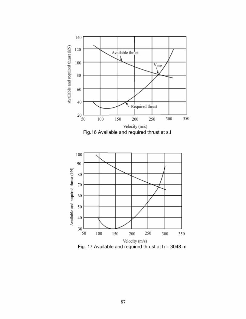
87
Fig.16 Available and required thrust at s.l
Fig. 17 Available and required thrust at h = 3048 m

88
Fig. 18 Available and required thrust at h = 4572 m
Fig.19 Available and required thrust at h = 7620 m

89
Fig. 20 Available and required thrust at h = 9144 m
Fig. 21 Available and required thrust at h = 10972 m The variations of Vs, (Vmin)e and Vmax are tabulated in Table 8 and presented in
Fig.22.

90
h (ft)
h (m)
Vs
(m/s) (Vmin)e
(m/s) T = Tcr
(Vmin)e
(m/s) T =Tclimb
Vmax
(m/s) T = Tcr
Vmax
(m/s) T =Tclimb
Vmax
(kmph) T=Tclimb
S.L 0 77.833 < Vs < Vs 258.711 269.370 969.7 10000 3048 90.579 < Vs < Vs 272.060 280.595 1010.1 15000 4572 98.131 < Vs < Vs 275.613 283.300 1019.9 25000 7620 116.292 < Vs < Vs 272.929 279.291 1005.4 30000 9144 127.278 < Vs < Vs 267.854 271.755 978.3 36000 10973 142.594 176.054 169.071 253.671 258.154 929.4 38000 11582 149.557 217.386 200.896 243.676 248.630 895.1 38995 11884 153.159 235.471 229.865 235.48 238.649 859.1 39220 11954 153.950 - 236.40 - 236.40 851.04 Table 8: Variations of Vmin and Vmax
Fig. 22 Variations of Vmin and Vmax with altitude 9.4 Steady climb
In this flight, the c.g. of the airplane moves along a straight line inclined to
the horizontal at an angle γ . The velocity of flight is assumed to be constant
during the climb. Since, the flight is steady, acceleration is zero and the
equations of motion can be written as:
T − D −W sin γ = 0 (96)
L −W cos γ = 0 (97)
To calculate the variation of rate of climb with flight velocity at different

91
altitudes, the following procedure is adopted.
(i) Choose an altitude.
(ii) Choose a flight speed.
Noting that CL = 2 W cos γ 2/ρSV , gives :
D DO 2
2W cosC = C + K
ρSV
Also
Vc = V sin γ
cos γ 2c2
V= 1 -
V
Using above equations yields the following equation for (Vc/V),
2
c cV VA + B + C = 0
V V
(98)
2 22
avail DO 22
kW 1 2kWA = ; B = - W; C = T - ρV SC -
1 2 ρV SρV S2
(99)
Since, altitude and flight velocity have been chosen, the thrust available
is read from the climb thrust curves in Fig.10. Further the variation of CDO
and K with Mach number is taken as in Eqs. (94) and (95).
(iii) Equation (98) gives 2 values of Vc/V. The value which is less than or equal to
1.0 is chosen as sin γ cannot be greater than unity. Hence,
γ -1c= sin (V / V) (100)
Vc = V sin γ (101)
(iv)This procedure is repeated for various speeds between Vmin and Vmax.
The entire procedure is then repeated for various altitudes.
The variations of (R/C) and γmax with velocity and with altitude as parameters
are shown in Figs. 23 and 25. The variations of (R/C)max and γmax with altitude
are shown in Figs. 24 and 26. The variations of V(R/C)max and Vγmax with altitude
are shown in Figs. 27 and 28. A summary of results is presented in Table 9.

92
h (ft)
h (m)
(R/C)max (m/min)
V(R/C)max (m/s)
γmax (degrees)
Vγmax (m/s)
0 0.0 1086.63 149.7 8.7 88.5 10000 3048.0 867.34 167.5 6.0 111.6 15000 4572.0 738.16 174.0 4.7 125.7 25000 7620.0 487.41 198.2 2.6 164.1 30000 9144.0 313.43 212.2 1.5 188.0 36000 10972.8 115.57 236.1 0.5 230.2 38000 11582.4 41.58 236.9 0.2 234.0 38995 11885.7 1.88 235.8 0.0 235.8 Table 9: Climb performance
Fig.23 Rate of climb vs velocity for various altitudes
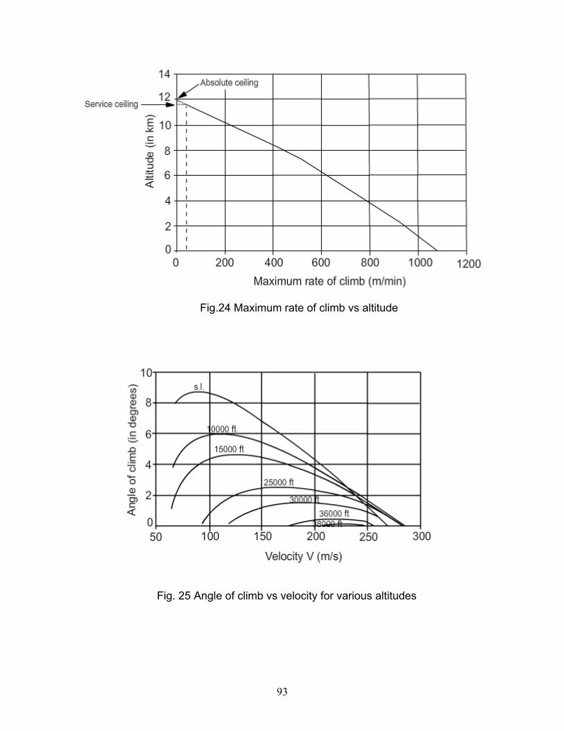
93
Fig.24 Maximum rate of climb vs altitude
Fig. 25 Angle of climb vs velocity for various altitudes

94
Fig. 26 Maximum angle of climb vs altitude
Fig. 27 Velocity at maximum rate of climb vs altitude

95
Fig.28 Velocity at maximum angle of climb vs altitude Remarks:
(i)The discontinuity in slope in Figs. 27 and 28 at high velocities are
due to the change in drag polar as the Mach number exceeds 0.8.
(ii) From Fig. 24, the absolute ceiling (at which (R/C)max is zero) is
11.88 km. The service ceiling at which (R/C)max equals 30 m/min is
11.68 km
9.5 Range and endurance
In this section, the range of the aircraft in a constant altitude and constant
velocity cruise is studied. Range is given by the formula:
-1 -11 22 2
DO DODO
2W 2W3.6 V K KR = tan - tan
ρV S C ρV S CTSFC KC
(102)
where, W1 is the weight of the airplane at the start of the cruise and W2
is the weight of the airplane at the end of the cruise.

96
The cruising altitude is taken as h = 10972 m. TSFC is taken to be constant
as 0.6hr-1. The variation of drag polar above M = 0.8 is given by
Eqs. (94) and (95).
W1 = W0 = 59175 × 9.81N
Wf = 0.205 ×W1
Allowing 6% fuel as trapped fuel, W2 becomes
W2 = W1 − 0.94 × Wf
The values of endurance (in hours) are obtained by dividing the expression
for range by 3.6V where V is in m/s. The values of range (R) and
endurance(E) in flights at different velocities are presented in Table 10 and
are plotted in Figs.29 and 30.
M
V
(in m/s)
CDO
K
R
(in km)
E
(in hours)
0.50 147.53 0.0159 0.04244 2979.0 5.61
0.55 162.29 0.0159 0.04244 3608.0 6.18
0.60 177.04 0.0159 0.04244 4189.6 6.57
0.65 191.79 0.0159 0.04244 4691.7 6.80
0.70 206.54 0.0159 0.04244 5095.6 6.85
0.75 221.30 0.0159 0.04244 5396.5 6.77
0.80 236.05 0.0159 0.04244 5599.8 6.59
0.81 239.00 0.0159 0.04256 5619.7 6.53
0.82 241.95 0.01592 0.04300 5621.6 6.45
0.83 244.90 0.01597 0.04388 5597.7 6.35
0.84 247.85 0.01604 0.04532 5544.1 6.21
0.85 250.80 0.01613 0.04744 5460.4 6.05
0.86 253.75 0.01624 0.05036 5349.3 5.86
0.87 256.71 0.01637 0.05420 5210.1 5.64
0.88 259.66 0.01652 0.05908 5051.1 5.40
Table 10: Range and endurance in constant velocity flights at h = 10972 m
(36000 ft)

97
Fig.29 Range in constant velocity flights at different flight speeds (h = 10972 m)
Fig.30 Endurance in constant velocity flights at different flight
speeds (h = 10972 m)
Remarks:
(i) It is observed that the maximum range of 5600 km is obtained at a
velocity of 239 m/s (860 kmph). Corresponding Mach number is 0.81.
which is slightly higher than the Mach number beyond which CDO and
K increase. This can be explained based on two factors namely

98
(a) the range increases as the flight speed increases (b) after Mcruise is
exceeded, CDO and K increase thus reducing (L/D)max.
(ii) The range calculated above is the gross still air range. The safe range
would be about two-thirds of this. In the present case, the safe range
would be 3733 km.
(iii)The maximum endurance of 6.85 hours occurs in a flight at
V = 206 m/s. (742 kmph). It can noted that the endurance is roughly
constant over a speed range of 190 m/s to 230 m/s.
9.6 Turning performance
In this section, the performance of the airplane in a steady, co-ordinated,
level turn is studied. The equations of motion in this case are:
T − D = 0
W - Lcos = 0
W
L sin =g
where, is the angle of bank.
These equations give:
2V
r =g tan
V gtan
ψ = =r V
L 1Load factor n = =
W cos
where,ψ is the rate of turn and r is the radius of turn.
The following procedure is used to obtain rmin and maxψ
1.A flight speed and altitude are chosen and the level flight lift coefficient
CLL is obtained as :
CLL 2
2(W / S)=
ρV
2. If CLmax / CLL < nmax, where nmax is the maximum load factor for

99
which the aircraft is designed, then the turn is limited by CLmax and
CLT1 = CLmax . However, if CLmax / CLL > nmax, then the turn is limited
by nmax, and CLT1 = nmaxCLL.
3. From the drag polar, CDT1 is obtained corresponding to CLT1 . Then,
2T1
1D = ρV S
2CDT1
If DT1 > Ta, where, Ta is the available thrust at that speed and altitude,
then the turn is limited by the engine output. In this case, the
maximum permissible value of CD in turning flight is obtained from :
aDT
2
TC =
1ρV S
2
From the above relation, the value of CLT is calculated as
DT DOLT
C -CC =
K
However, if DT1 < Ta , then the turn is not limited by the engine output
and the value of CLT calculated in step (2) is retained.
4. Once CLT is known, the load factor during the turn is determined as
LT
LL
Cn =
C
Once n is known, the values of , r and ψ can be calculated using the
equations given above.
The above steps are repeated for various speeds and altitudes. A
typical turning flight performance estimation is presented in Table 11. In
these calculations, CLmax = 1.4 and nmax = 3.5 are assumed. The variation
of turning flight performance with altitude is shown in Table. 12. Figures
31, 32, 33, 34 respectively present (a) radius of turn with velocity and with
altitude as parameter, (b) minimum radius of turn with altitude, (c) rate of
turn with velocity and with altitude as parameter and (d) maximum rate of
turn with altitude.

100
V
(m/s)
n
CLT
(degrees)
r
(m)
ψ
(rad/s)
78.83 1.026 1.4000 12.892 2767.70 0.0285
98.83 1.612 1.4000 51.670 787.21 0.1255
118.83 2.331 1.4000 64.596 683.63 0.1738
138.83 2.813 1.2376 69.173 747.41 0.1858
158.83 2.993 1.0062 70.482 911.60 0.1742
178.83 3.089 0.8192 71.112 1115.38 0.1603
198.83 3.080 0.6607 71.053 1383.50 0.1437
218.83 2.930 0.5189 70.045 1772.43 0.1235
238.83 2.573 0.3826 67.132 2452.36 0.0974
241.83 2.494 0.3617 66.363 2609.20 0.0927
Table 11 Typical turning flight performance at sea level
Fig.31 Radius of turn vs velocity at various altitudes

101
Fig.32 Velocity at rmin vs altitude
Fig. 33 ψ vs speed at various altitudes

102
Fig. 34 Velocity at maxψ vs altitude
h (m)
rmin (m)
Vrmin (m/s)
maxψ
(rad/s)
ψmaxV
(m/s) 0.0 666 126.8 0.1910 127.8 3048.0 945 132.6 0.1410 133.6 4572.0 1155 135.1 0.1170 136.1 7620.0 1971 138.3 0.0731 165.3 9144.0 3247 151.3 0.0513 187.3 10973.8 8582 211.0 0.0256 231.0 Table 12 Turning flight performance Remarks:
1. The maximum value of maxψ is 0.191 and occurs at a speed of 127.8 m/s
at sea level.
2. The minimum radius of turn is 666 m and occurs at a speed of 126.8 m/s
at sea level.
3. The various graphs show a discontinuity in slope when the criterion,
which limits the turn, changes from nmax to thrust available.

103
9.7 Take-off distance
In this section, the take off performance of the airplane is evaluated. The
take-off distance consists of take-off run, transition and climb to screen
height. Rough estimates of the distance covered in these phases can be
obtained by writing down the appropriate equations of motion. However, the
estimates are approximate and Ref.4 chapter 5 recommends the following
formulae for take-off distance and balance field length based on the take-off
parameter.
This parameter is defined as:
LTO
W / STake -off parameter =
σC (T / W) (103)
where, W/S is wing loading in lb/ft2, CLTO is 0.8 × CLland and σ is the density ratio
at take-off altitude.
In the present case:
2 2LTO
W= 5195 N/ m = 108.2 lb / ft ; C = 0.8 × 2.7 = 2.16; σ = 1.0 (sea level)
S
T 2 × 97.9 kNand = = 0.3373
W 59175 × 9.81
Hence,
Take-off parameter = 108.2
= 148.861.0 × 2.16 × 0.3373
(104)
From Ref.4, chapter 5, the take off distance, over 50’, is 2823 or 861 m. The
balance field length for the present case of two engined airplane is 6000 or
1829 m.
Remark:
It may be noted that the balance field length is more than twice the take off
distance.

104
9.8 Landing distance
In this section the landing distance of the airplane is calculated. From Ref.4
chapter 5, the landing distance for commericial airliners is given by the formula
landLmax
W 1S = 80 + 1000 ft
S σC
(105)
where, W/S is in lbs/ft2. In the present case:
(W/S)land = 0.85 × (W/S)takeoff = 0.85 × 108.5 = 92.225lb/ft2
CLmax = 2.7
σ = 1.0
Hence,
land
1S = 80 × 92.225 + 1000 = 3732 ft = 1138 m
1.0 * 2.7 (106)
9.9 Concluding remarks
1. Performance of a typical commercial airliner has been estimated for
stalling speed, maximum speed, minimum speed, steady climb, range,
endurance, turning, take-off and landing.
2. The performance approximately corresponds to that of B737-200.
3. Figure 35 presents the variation with altitude of the characteristic velocities
corresponding to :
stalling speed, Vs
maximum speed, Vmax
minimum speed as dictated by thrust, (Vmin)e
maximum rate of climb, V(R/C)max
maximum angle of climb, γ maxV
maximum rate of turn, ψmaxV
minimum radius of turn, Vrmin

105
Fig. 35 Variations of characteristic velocities with altitude
10 Acknowledgements The first author(EGT) thanks AICTE for the fellowship which enabled him to carry out the work at IIT Madras.
References 1. http://www.cfm56.com/engines/cfm56-5c/tech.html 2. http://www.lissys.demon.co.uk/samp1/ 3. Harris C.H. “NASA supercritical airfoils – A matrix of family- related airfoils”
NASA TP 2969 , March 1990. (This reference can be downloaded from the
site “NASA Technical Report Server (NTRS)”)
4. Raymer, D.P. “Aircraft design: a conceptual approach” AIAA educational
Series, Fourth edition (2006).
5. Web course under Aerospace Engineering of NPTEL entitled “Airplane design(Aerodynamic) ” by Tulapurkara E.G. (www.nptel.iitm.ac.in)

106
6. Roskam J.”Methods for Estimating Drag Polars of Subsonic Airplanes” Roskam Aviation and Engineering Corporation, Ottawa (1973). 7. Lebedinski. A.A. “Aircraft design – Part 1 - parametric studies” Published by
I.I.Sc Bangalore, (1971).
8. Jenkinson L. R., Simpkin P. and Rhodes D. “Civil jet aircraft design”
Arnold, (1999).
9. Hoerner S. F. “Fluid-dynamic drag”, published by Hoerner Fluid Dynamics,
Brick Town, NJ, (1965).
10. Wood K.D. “Aerospace vehicle design vol I.& II” Johnson Pub. Co Boulder
Colorado (1966). 11. Perkins, C.D. and Hage R.E. “Aircraft performance, stability and control” Wiley, (1949). 12 Abbott I. H. & Von Doenhoff A. E. “Theory of wing sections”, Dover, (1959).
13. Roskam, J “Airplane design Vol. I –VIII” Roskam aviation and Engg. Corp.
Ottawa, Kansas (1989), (2007).
14. Webcourse under Aerospace Engineering of NPTEL entitled “Flight dynamics – II – Airplane stability and control” by Tulapurkara E.G. (www.nptel.iitm.ac.in) 15. Dommasch,D.O. Sherby, S.S. and Connolly, T.F. “Airplane
aerodynamics” Pitman (1967).
16. Torenbeek. E. “Synthesis of subsonic airplane design” Delft University
Press, (1981).