An Examination of the Impact of Rent Control on Mobile Home

An Examination of the Impact of Rent Control on Mobile Home Prices in California

By

Diehang Zheng, Yongheng Deng, Peter Gordon, and David Dale-Johnson†

Lusk Center for Real Estate University of Southern California

Los Angeles, CA 90089-0626

September, 2006

Abstract

This study examines the impact of rent control of mobile home parks in seven counties of California between 1983 and 2003. We assembled an extensive and timely data set and, thus, were able to test more carefully specified econometric models than had been employed in prior studies of California mobile-home rent control. We find that the nature of the rent control regime differentially impacts mobile home prices: the imposition of rigid rent control, rent control without vacancy decontrol, leads to higher growth rates in resale prices. While a flexible regime, or rent control with vacancy decontrol, results in lower growth rates in resale prices. This is consistent with economic theory, suggesting that the imposition of rigid rent control will lead to the capitalization of future rent savings when a coach is sold. That is, the buyer will not only pay for the coach but also for the net present value of the expected savings associated with the future legally constrained pad rent obligations to the landlord.

† The authors are grateful for helpful comments from John Quigley, and participants at the International Conference for Real Estates and the Macroeconomy at Beijing, Hoyt Fellows Research Seminar at the Homer Hoyt Institute, and the Western Regional Science Association Annual Conference at Santa Fe. The authors also gratefully acknowledge the Pacific Legal Foundation for providing the mobile home data and the financial support from the Lusk Center for Real Estate at USC for this study.

1

1. Introduction

This study uses a unique micro-level mobile home transactions data set to analyze the impact

of mobile home rent control in California. Is so doing, we hope to advance our understanding of

the impact of price controls.

The social and economic impacts as well as the legal implications of price controls in the

rental housing market have been debated extensively among economists and legal scholars. There

appears to be widespread agreement on a number of points. Most economists agree that “a ceiling

on rents reduces the quantity and quality of housing available” (Alston, Kearl, and Vaughan,

1992).1 While some renters benefit from lower rents, there are also costs (Olsen, 1972).2 Severe

rent controls can cause undersupply in the apartment rental markets, and increase the search costs

for tenants (Arnott and Igarashi, 2000). Below-market prices, if enforced, create opportunities for

non-price rationing. Potential renters are obliged to invest time and effort chasing down access to

the limited supply. These resource expenditures do not accrue to any sellers and cannot be

converted to product and thus become a “deadweight” efficiency loss.

Also, maintenance of the existing housing stock and investment in new stock are expected to

decline. In fact, abandonment of housing stock by owners has been observed. Housing

conversions and demolitions have also been attributed to rent controls, an outcome further

reducing the housing stock. Additional efficiency losses come from renters failing to adjust their

housing consumption even though their circumstances change so they can hold on to their rent

controlled units. (See Gyourko and Linneman, 1988, and Glaeser and Luttmer, 2003, for a

thorough discussion of such effects for the case of New York city.) In addition, higher-income

households are likely have an advantage in tracking valuable information on available units.

Thus, equity gains from rent controls have seldom been realized by those most in need such

benefit, suggesting that rent control has not been a policy useful for lower-income households

1 Alston, Kearl, and Vaughan (1992) reported that from their survey of a stratified random sample of 1,350 economists employed in the United States, more than three-quarters of the respondents agreed with the above statement. 2 One seminal study of rent control in New York City estimated that the costs to property owners are two times the benefits to renters (Olsen, 1972).

2

that seek affordable housing (Quigley, 2002). For many reasons, then, rent controls preclude land

and housing markets from doing what they are supposed to do, namely allocate scarce resources

to their highest and best uses in light of ever changing wants, opportunities and constraints. Some

existing studies found that a well-designed rent control regime could improve the unrestricted

equilibrium of an imperfect market (Arnott, 1995). Rent control is preferred when the market

distortion is the unavailability of insurance against a sharp, unanticipated rent rise. However,

economists disagree on the net social effect of rent controls, for example, whether rent controls

might affect increased homelessness by reducing the supply of rental units (Tucker, 1989,

Quigley, 1990, HUD, 1991, Early and Olsen, 1998).

Rent control policies have caught the attention of legal scholars and have been extensively

litigated. Legal scholars have debated whether some rent control regulations have violated the

Fifth Amendment’s Takings Clause. In Yee v. City of Escondido, Cal. (90-1947), 503 U.S. 519

(1992), the Supreme Court affirmed a Superior Court decision rejecting the argument that the

ordinance effected a physical taking by depriving park owners of all use and occupancy of their

property and granting to their tenants, and their tenants' successors, the right to physically

permanently occupy and use the property. The Supreme Court ruled that the argument that rent

control ordinances benefit current but not future property owners has “nothing to do with whether

it causes a physical taking.” Since then, some legal scholars have nevertheless argued that certain

rent controls constitute a regulatory taking because the regulation has unfairly singled out some

property owners to bear a burden that should be borne by the public at-large. (See Rubinfeld,

1992, and Radford, 2004, for a discussion.)

A unique aspect of the mobile home industry is the separate ownership of the coach and the

pad where the coach is located; i.e., the mobile homeowner owns only the coach unit and rents a

pad in a mobile home park on which she parks her (not-so-mobile) home. If the rent of the pad is

constrained to be below market rents, coach owners are hypothesized to be able to sell the coach

for more than it would be worth without rent control, thereby capitalizing the rent savings arising

3

from rent control. The framework of separate ownership of coach unit and pad provides a unique

opportunity to explicitly test the economic impact of rent control policy.

Several studies by Hirsch (1988), Hirsch et al (1988) and Hirsch and Rufolo (1999) have

analyzed capitalization of the effects of rent control on coach unit values. Using straightforward

hedonic modeling techniques and relatively small samples, the authors demonstrated that the

savings from pad rent controls are capitalized.

In this study, we propose an extended economic model using a large sample of about

200,000 mobile home transaction records from January 1983 to May 2003 from seven counties in

California.3 The coach transaction records include information on each coach’s quality (brand,

length, and width), age, address, original sale price, last sale price, last sale date, etc.

The purpose of this study is twofold. First, we intend to provide a more explicit and

comprehensive measure of the economic impacts of rent controls through an analysis of micro

transactions data. Second, we seek to provide evidence on the extent to which mobile home rent

control constitutes a regulatory taking.

The remainder of this paper is organized as follows: Section two summarizes the unique

characteristics of the mobile home market and rent controls in such markets. Section three

describes our methodology for measuring rent control capitalization. Section four discusses the

data; Section five presents our empirical results. The last section offers concluding remarks.

2. The Mobile Home Industry

In 2003, almost 9 million of the nation's 121 million housing units were mobile homes. This

was 7.4 percent of the housing stock, up from 6.5 percent of the housing stock in 1987. Of the

more than 338 thousand mobile homes added to the U.S. housing stock in 1999, more than 10

percent were added in the western states. As the number of Americans living in mobile homes

increases, more attention is being paid to mobile home parks, their management and associated

3 The data are maintained by the California Department of Housing and Community Development (HCD).

4

public policies. Among the issues of great interest are the effects of various types of mobile home

rent control.

The imposition of rent controls in many California jurisdictions has been shown to explain

declining shipments of mobile homes to California (Hirsch and Rufolo, 1999). More up-to-date

time series transactions data for California also show that from 1983-2003 (through the month of

May), the number of mobile homes subject to rent controls increased. Figures 1a through 1c show

the transaction data in our sample by various mobile home descriptors including Total Traded

Square Feet, Total Traded Value (constant dollars), and the Number of Transactions.

Rent control policies and by-laws vary in scope and severity. Flexible rent control regimes

allow vacancy decontrol while more rigid regimes permit rent increases tied to one of a variety of

cost-of-living indices. Rent control regulations in many cities have gone through cycles of control

and decontrol, in some cases resulting in various vintages of the stock being grandfathered. A

visible result is that some cities have neighborhoods with well-kept free-market rental housing

adjacent to poorly maintained rent controlled housing.

Rent control systems are most well known for having been imposed on traditional

multi-family rental housing units where the landlord owns the land and the building and rents

individual units to tenants using formal or informal leasing arrangements. Legal systems have

evolved to define the property rights of landlords and tenants. Rent controlled systems often

“piggy-back” on these systems as security of tenure is deemed critical if landlords are permitted

to increase rents when a unit is vacated.4

In contrast, in mobile home parks, the site (“pad”) is rented to the tenant who either acquires

the mobile home from a prior tenant or buys a new mobile home which is then assembled on-site.

The curious distinction from the more common rent control of multi-family apartment units is

that in a mobile home park the landlord owns the land (the pad) and the tenant owns the

improvements (the coach). If there is no vacancy decontrol (ability on the part of the landlord to

4 In more rigid rent control systems, controls are tied to the unit rather than the tenant.

5

adjust the pad rent to the market rent when the coach is sold), the net present value of the

anticipated future rent savings should be capitalized into the sales price of the coach if it stays in

place. And usually it does as mobile homes are seldom moved once they are located on a pad.

This unique aspect of rent control for mobile home parks has been the subject of some empirical

analysis. Rent control systems for mobile home parks provide an opportunity to investigate the

economic impact of the rent control policy on the tenants of mobile parks (i.e., the mobile coach

owners).

Rapidly rising housing and land prices in California explain rising pad rents in many of the

state’s mobile home parks. As a consequence, renters in many jurisdictions responded by

launching efforts to have rent controls enacted into law. In 2003, ninety seven California cities

and eight counties had some sort of mobile home rent control.

In a series of papers published in the late 1980s, Hirsch and his colleagues (Hirsch, 1988,

and Hirsch and Hirsch 1988) examined the impacts of rent controls on mobile homes in

California. As alluded to previously, their analysis rests on the insight that ownership of mobile

home living space is divided between the owner of the coach and the owner of the land, which is

then leased to coach owners. Therefore, a coach atop a rent-controlled pad can be expected to sell

at a premium. Hirsch et al’s studies contain estimates of these values. Basing their analysis on a

relatively small sample of observed transactions from the mid-1980s, they estimated that sales

prices were boosted by 32 percent because of rent controls, other things equal.

An updated analysis by Hirsch and Rufolo (1999) focused on a single mobile home park in

Oceanside, California. A hedonic regression based on a sample of 90 mobile home sales over the

period 1986-1992 found that, other things equal, rent controls explain a price premium of eight

percent.

More recently, Quigley (2002) presented an economic analysis of mobile home rent control

based on a single mobile home park in San Rafael, California. The study documented the

arms-length sales of 40 mobile homes in that park during a three-year period. The study estimated

6

the average value of the rent control premium varied from $16 to $160,000. Price premiums for

coaches enjoying rent control benefits in this study averaged an impressive 366 percent.

3. The Model

This section lays out the methodology adopted to model the capitalization of rent control.

The approach to measuring housing price appreciation has advanced as a consequence of work by

Bailey, Muth and Nourse (1963), Case and Shiller (1989), Case and Quigley (1992) and Harding,

Rosenthal and Sirmans (2005) among others. In this paper, we employ repeat sales price indexes

in the mobile home market in California to examine the impact of variation in rent control

policies among jurisdictions, while controlling the socio-economics of the neighborhoods in

question and of the physical attributes of the coaches themselves.

As discussed in previous sections, due to the separate ownership of the mobile home coach

and the pad where the coach parks, coach owners in a jurisdiction with rigid rent control can

capitalize the anticipated savings from controlled rents when they sell their units. Our model

extends the work by Bailey, Muth and Nourse (1963) and Case and Shiller (1989) by

decomposing the mobile home repeated sale house price differential into mobile home property

value appreciation and the capitalization of the mobile home park rent control premium. 5

Consider a mobile home coach which is observed to have been purchased and sold in periods

t and t τ+ , respectively. The purchase price is

' '

, ,j t t ty zt j t

j

P A x e e eα β δ γ= ∏ (1)

where A is the parameter to capture the common factors’ effect on all the units in the study;

( ), 1,...,j tx j q= and ty are a set of property’s hedonic characteristics observed at time t; tz

is a vector of binary regulatory features indicating different rent control regimes; α , β and δ

5 Our decomposition process is similar to the model proposed by Harding, Rosenthal and Sirmans (2005) in which they modify the repeated sales house price index model by decomposing the housing price appreciation into the components of capital depreciation and impact of housing maintenances.

7

are shadow prices for hedonic characteristics, and regulatory features respectively; tγ is a vector

of parameter for price index capturing aggregate price appreciation.

Let the price vary over time, from equation (1) the selling price at time t τ+ will be

' '

, .j t t ty zt j t

j

P A x e e eτ τ τα β δ γτ τ

+ + ++ += ∏ (2)

From equations (1) and (2), the price ratio and the log price ratio, respectively, between

t τ+ and t can be expressed as follows:

( ) ( ) ( )' ',

,

,j

t t t t t ty y z zj tt

jt j t

xP e e eP x

τ τ τ

α

β δ γ γττ + + +− − −++⎛ ⎞

= ⎜ ⎟⎜ ⎟⎝ ⎠

∏ (3)

and

( ) ( )( ) ( ) ( ) ( )' ', ,ln ln ln .t

j j t j t t t t t t tjt

P x x y y z zPτ

τ τ τ τα β δ γ γ++ + + +

⎛ ⎞= − + − + − + −⎜ ⎟

⎝ ⎠∑ (4)

If we assume the hedonic characteristics and regulatory attributes remain constant between

the two transactions, i.e. , , ,j t j tx xτ+ = t ty yτ+ = , and t tz zτ+ = , then equation (4) can be

reduced to

( ) ,t tt tP Pe τγ γτ

+ −+ = (5)

or the price change reflexes only the appreciation of market value of a constant quality property.

This is exactly the repeat house price index model developed by Bailey, Muth and Nourse (1963)

and Case and Shiller (1989).

Suppose the binary regulatory attributes between t and t τ+ change from z to *z , as a

consequence of the adoption of a rent control ordinance during the time between the two

transactions. The transacted price growth can be decomposed into constant quality property price

appreciation and the impact of change in regulatory attributes.

* '( ) ( ) .t t z z

t tP Pe eτγ γ δτ

+ − −+ = (6)

8

Let’s assume the property price follows a log normal distribution6. We can test the above

specifications by taking logarithms and rearranging equations (5) and (6), such that,

( )ln( ) ,tt t

t

PPτ

τγ γ ε τ++= − + (7)

and

( )* 'ln( ) ( ) ,tt t

t

P z zPτ

τγ γ δ υ τ++= − + − + (8)

respectively, where ( )ε τ and ( )υ τ are random error terms following a normal distribution with

a diffusion variance which increases with the time span, τ , between the two transactions.

For the case of mobile homes, provided all the other characteristics except for the rent

control policy are time-invariant, the problem of selecting the proper specification of functional

form or how qualitative and quantitative characteristics determine housing price growth has been

eliminated. This elimination enhances the reliability of the estimates for the price index, γ .

For a sample of mobile homes that are transacted at various time periods, we obtain

( )' 'ln( ) ( ) ,tt t

t

P D RC RCPτ

τγ δ υ τ++= + − + (9)

where D is a vector of indicator variables taking values of -1, 0, or 1, determined by both

purchase and sale of each property7; γ is price index vector; RC is a vector of indicator variables

for various rent control regimes,8 and the modified repeated sales house price index model

expressed in equation (9) allows us to decompose the capitalization of any rent control premium

from property value appreciation.

Yet, Redfearn (2005) has pointed out an additional source of significant bias in aggregate

indexes is the ignorance of local dynamics. Case and Quigley (1992) acknowledged that it is

6 The same assumption was implied by Bailey, Muth and Nourse (1963), Case and Shiller (1989), and Case and Quigley (1992). 7 The indicator variable takes value of -1 if the first transaction of the property occurs in period t; and takes value of 1 if the second transaction of the property occurs in period t τ+ ; and takes value of 0 for all the other periods. 8 1 indicates the property is under rent control; 0 means no rent control policy adopted.

9

appropriate to control statistically for the varying characteristics of properties in inferring price

trends. Clapham et al. (2004) compared the stability of the repeat sales index and the hedonic

index and found that character-based hedonic indexes appear to be substantially more stable than

repeat-sales indexes. Hence we can modify equation (9) such that

( ) ( )( ) ( ) ( ) ( )

( ) ( )

' ', ,

''

ln ' ln ln

' ,

tj j t j t t t t t

jt

t t

P D x x y y RC RCP

D Z RC RC

ττ τ τ

τ

γ α β δ μ τ

γ θ δ μ τ

++ + +

+

⎛ ⎞= + − + − + − +⎜ ⎟

⎝ ⎠

= + + − +

∑

(10)

where θ is a vector of parameters which contains both α and β ; Z (contains x and y) is a

vector of control variables capturing the location effect (measured by county), as well as hedonic

effects (coach structure such as single-, double-, or triple-width, size, and neighborhood quality,

etc.). This additional vector measures the proportional effects of location and the coach’s

amenities on the price growth rate.

4. The Data

In this research, twenty years of transactions data for mobile homes in seven counties of

California (Los Angeles, Orange, Riverside, San Bernardino, San Diego, Santa Clara and

Ventura) were made available to us. After geo-coding and matching with census tracts, there were

201,228 records from the period beginning of January 1983 and ending in May 2003. As we

wished to create hybrid repeat-sale indexes, our focus is on sales of coaches for which there are

two transactions, the first purchase and one resale, thus records for single sales were removed

from the data set9. Other records were eliminated because of incomplete city or mobile home park

(Park ID) information. Outliers were also removed. 10 These modifications left a 20-year

population of 137,221 sales in the data set.

9 For those properties with more than two transactions, only one resale record is included in the analysis. 10 Records with incomplete geographic information and the top and bottom 1 percent of records based on the variables Original Sales Price (Constant 1996 dollar), Resale Price (Constant 1996 dollar), Size and Average Annual Growth

10

Each record in the original data set is a mobile home transaction and includes the county,

city, address, mobile home park name and ID, the original sale price for the new structure and

resale price, the dates of sale (year, month, and day), and measures of other attributes of the unit

such as model year, manufacturer, width, length, and type (single, double, or triple) and so on.

These data were combined with census data by census tract, including median household income,

changes in median household income, vacancy rate, proportion of the elderly (≥ 65 years old),

unemployment rate, and proportion of households with public assistance income, etc. We assume

the census tract descriptors apply to the population living in mobile home parks. Finally,

city-specific mobile home park rent control information was incorporated in the merged data set,

including an indicator of the nature of the rent control regime.11 Table 1 defines each of the

variables included in the data set.

There are 201 municipalities in the seven counties included in this study, among which 49

cities have a rent control ordinance. As many as 48,664 transactions in the data set (35.5 percent)

were actually in jurisdictions where there was rent control. Among those, around half were under

rigid rent control. From Figures 1a through 1c, we can see that the share of transactions as

measured by square footage, value and number has increased significantly over the twenty-year

period under study. Table 2 reveals in the right-hand column that the share of rent controlled units

among the total mobile home transactions in the seven counties grew from almost thirteen percent

in the early 1980’s to more than forty percent in 2003; moreover, the growth of those under rigid

rent control outpaces the growth of transactions of units under flexible rent control since the

middle 1990s. The change in the share of the square footage traded and the value traded

attributable to rent-controlled units is of the same order. Table 3 presents the annual growth rates

in rent-controlled units among the transactions as measured by square footage, value and number.

Rate were removed from the data set. We also explored the impact of focusing on properties where 0.5 < (Constant Resale Price/Constant Original Sales Price) < 3.0. We found that the results were robust to the imposition of this constraint. See Table 1 for descriptions of the variables. 11 For cities with rent control, dummy variables were including starting in the quarter in which rent control was implemented. We also included a dummy variable that indicates whether or not there is vacancy decontrol. No vacancy decontrol reflects a more rigid rent control regime.

11

The growth rates were 13.02, 13.19 and 13.17 percent, respectively. Clearly, rent control policies

in the mobile home marketplace in California are taking on increasing importance.

Table 4 provides descriptive statistics for the continuous covariates for the complete data set

as well as for each county. The original sale price varies from an average of $36,940 (San

Bernardino) to $46,410 (Santa Clara); while the average resale price varies from $22,085 (San

Bernardino) to $54,441 (Santa Clara). The average original sale price and resale price of the

seven counties are $40,775 and $34,118 respectively. Mobile homes are less likely to keep up

with rapid residential land market appreciation. Declines in the values of mobile homes are more

common than for “stick-built” houses because the land component is often not part of the selling

price.12

Census tract variables including Median Household Income, Proportion of Households with

Public Assistance Income, and Proportion of Persons ≥ 65 Years Old were collected and also

reported in Table 4. Other census tract-level variables, including Changes in Median Household

Income, Vacancy Rate, and Unemployment Rate, were collected but were ultimately not of

significance in the analysis so their summary statistics are not reported here.

Riverside county had the lowest median household income ($33,149) accompanied by the

highest elderly population (24.4 percent). Santa Clara county was at the other extreme with the

highest median household income ($52,492) and was tied with two other counties for the second

lowest proportion of elderly population (11.4 percent). Perhaps surprisingly, Los Angeles county

had the lowest proportion of elderly at 10.3 percent. San Bernardino and Riverside counties had

the highest proportion of households benefiting from public assistance (9.0 and 8.6 percent,

respectively) while Ventura and Orange counties had the lowest (5.0 and 5.2 percent,

respectively).

We ultimately used the census information to segment the data set. Specifically, high- (or

low-) income is defined by whether the census tract median household income is above (or

12 A more suitable comparable for mobile home sales would be sales of stick-built houses on leased land.

12

below) the median census tract household income in the corresponding county. High- (or low-)

elderly population proportion is defined by whether the census tract older population proportion

is above (or below) the median census tract elderly population proportion in the corresponding

county.

The smallest mobile homes are in San Bernardino and Los Angeles counties as measured by

Unit’s Size (1,093 and 1,094 square feet) while the largest are in Orange county (1,199 square

feet). Ventura and San Diego counties have the oldest units (20.85 and 20.75 years, respectively)

while Riverside county has the youngest (16.14 years).

Table 5 provides descriptive statistics for the sample’s categorical covariates. Double-width

mobile homes are the most common as indicated by a market share of almost 70 percent for the

type “Double”. The second biggest share is for single-width or the “Single” category at a market

share of 26 percent; triple-width or the “Triple” category represent the luxury high-end mobile

homes and have a five percent share of the market. The market share of double-width in Orange

county is about 15 percentage points higher than in Los Angeles, while the market share of

single-width is about 15 percentage points lower perhaps reflecting stage of the evolution of the

mobile home market as well as the role of mobile homes as a housing choice when the homes

were originally sold and the mobile home parks developed.

As noted earlier, a number of qualitative (“dummy”) variables were created which are

critical to the analysis. First, communities are identified in which rent control of mobile home

parks was present. Second, the policy is classified as rigid (by-laws which do not permit vacancy

decontrol) or flexible (by-laws which permit vacancy decontrol), depending on whether or not

vacancy decontrol is permitted. Then transactions within these jurisdictions were identified

accordingly. Third, the first transaction after the adoption of a rent control policy is also

indicated. The results of these classifications for the aggregate data set also appear in Table 5.

The prevalence of rent control ordinances varies dramatically among the seven counties.

While in the aggregate, less than five percent of the transactions in Orange county were in

13

rent-controlled parks, 82.7 percent of the transactions in Ventura county were in rent-controlled

parks. As noted earlier, there was significant variation in these percentages between 1983 and

2003 with an increasing number and share of mobile home units being regulated by rent control

policies over time. Of the 35.5 percent of mobile home transactions in our data set that are within

rent controlled jurisdictions, roughly half of them are in jurisdictions with flexible rent control

regimes and the rest are in jurisdictions with rigid rent control regimes.13

5. Empirical Results

We had a much larger and more comprehensive sample available to us than was employed in

Hirsch (1988), Hirsch et al (1988, 1999) or Quigley (2002). As noted, we focused on 137,221

observations collected from over twenty years of mobile home transactions between 1983 and the

early part of 2003. The ultimate transaction data base included only repeat- or multiple-sales

along with descriptive information about the coach. Each sale was geo-coded permitting the

census tract variables including Median Household Income (constant 1996 dollar), Proportion of

Households with Public Assistance Income and Proportion of Persons ≥ 65 Years Old to be

appended to each record. The first two are proxies for local amenity values as well as demand,

while the third is a proxy for one of the components of demand for mobile home units -- as many

older households choose mobile homes as a cost-effective housing choice in retirement.

Our working hypothesis was that because rigid rent control policies allow coach owners to

pass on future pad rent savings to subsequent owners of the coach, prices of coaches in these

communities will increase more rapidly or decrease less rapidly than the prices of coaches in

communities without rent control or flexible rent control. To be sure, this is actually a net effect.

Buyers value protections from rent increases but also may be wary of owning property in cities

13 Rent control regimes may become less rigid or more rigid through time as policies evolve due to the changing economic and political environment. We were able to identify regimes which are currently rigid (no vacancy decontrol permitted) or flexible (vacancy decontrol permitted). In order to ascertain whether today’s regime accurately reflected the nature of the regime since 1983, we surveyed every city in our data set (201). We received 55 responses in total with 20 of them from cities with rent control in place. The results of the survey supported the approach taken. We inferred that the results of the survey could be extrapolated to the full sample.

14

with governments that have shown themselves to be ready to place limits on property rights.

This suggests that any weak form of rent control could be associated with especially ambiguous

expectations. It is not clear which effect would dominate.

Thus, if rent control or the rigidity of the rent control regime influences the rate of change of

coach prices, the relevant estimated coefficient will be positive and significant. Moreover, the

biggest beneficiary is the first generation of mobile home owners when the rent control policy

is/was adopted. For the standard case, the following coach owners are not able to realize a

comparable benefit because they have paid for most of the premium for rent control upfront.

Nevertheless, in cases when future appreciation had been underestimated, there would be

additional rents to be further capitalized in the later transactions.

Table 6 presents the results of GLS estimation of equations (9) and (10).14 In model (1),

mobile homes values are positively influenced if rigid rent control policies are adopted but those

will decrease when flexible rent control policies are adopted. This set of relationships still holds

when the proportional effects of other hedonic factors have been considered in model (2).

Riverside and San Bernardino have the lowest growth rates, while Ventura outperforms all the

other counties. The larger luxury units experience higher appreciation than smaller ones. The

coaches in the neighborhoods with a higher proportion of households with public assistance

suffer from lower growth rates. For rent control policies, the first generation mobile home owners

under rent control benefit from the adoption of rigid rent control ordinances (rent control without

vacancy decontrol), but they experience a net loss, ceteris paribus, from flexible rent control (rent

control with vacancy decontrol), as suggested may be possible in our theoretical discussion.

14 We adopt GLS estimation approach to address the problem of heterogeneity due to the diffusion process of the error terms specified in equations (9) and (10). Following Case and Shiller (1989) and Deng, Quigley and Van Order (2000), we first estimate equations (9) and (10) by OLS. In the second stage, we estimate a diffusion process of the variance by

regressing the square term of residuals, 2ε , collected from the first stage OLS regression on a quadratic function of time span between the two sales, such that ( )2 2

1 2ε τ β τ β τ ω= + + , where τ is the duration between original sale and resale (measured in quarters), and ω is a normally distributed error term. In the third stage we re-estimate the mobile home price index model using a GLS estimation approach weighted by the square root of the estimated diffusion variance, ( )ε̂ τ , obtained from the second stage.

15

Our results also show that for the following generations of tenants, rigid rent control policy

is no longer a significant factor in determining the resale price, while a flexible rent control

regime may continue contributing to lower resale price.

Because rigid rent control practically freezes real rents paid, in a market where demand

increases in the long run such as in the market for mobile homes, the longer this restriction is in

force, the bigger would be the price gap, between the controlled units and the uncontrolled units.

Model (3) replaces the simple dummy variable “adoption of rent control without vacancy

decontrol” by the interactive variable “adoption of rent control without vacancy decontrol ×

number of years under rent control at time of transaction”. The interactive variable is significant

and keeps the same sign as its simple dummy counterpart in model (2). It shows that the adoption

of rigid rent control will push up the mobile home value by 1.5 percent per year till the first

transaction after the introduction of the policy. Also, because of different rent control adoption

schedules, San Diego and Santa Clara have different signs for their dummy variables in this

model compared to model (2).

Figure 2a provides the plot of dependent variable, Log (resale price/original price) or

Log-Ratio, for different counties. Santa Clara has the highest growth rate and the lowest variance;

Riverside has the lowest growth rate with the greatest variance. Hence, it is inappropriate to treat

the seven counties equally at the aggregate level.

Similarly, Figure 2b and 2c give the plots of Log-Ratio for different structure groups (single,

double, and triple), and for different rent control groups. Due to the difference among the

subgroups a proportional model as in Equation (10) is adopted.

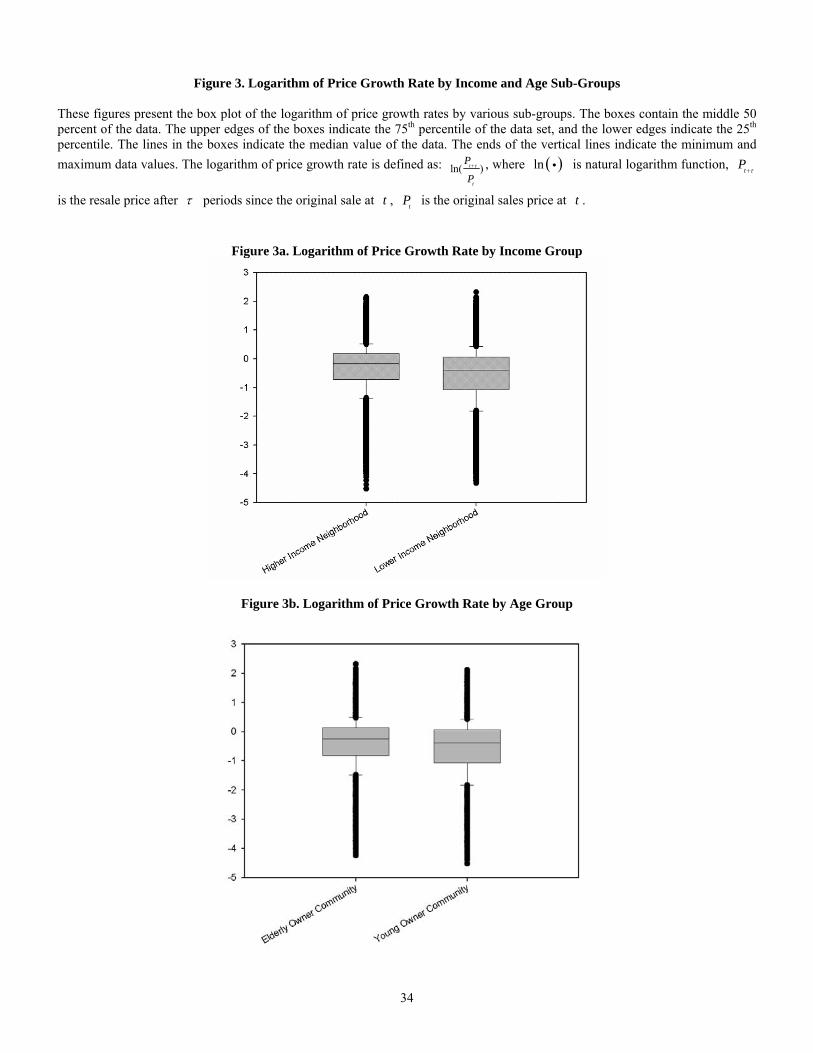
From a policy perspective it might be valuable to know which income-age group can benefit

the most from a rent control policy, and also, who might suffer the most. Figure 3a and 3b present

the plots of Log-Ratio by different median household income census tracts and different

proportion of elderly population census tracts. The differences between higher and lower income

communities, as well as older and younger communities are visible. Hence, we refine the full

16

sample and re-estimate the index with proportional location and hedonic factors for each

income/age group, in order to estimate rent control’s impact under different scenarios.

The re-estimated results for different median household income census tract groups are

presented in Table 7a. Adoption of rigid rent control leads to higher increase in resale price for

coaches in wealthier communities, but homeowners in poorer communities suffer less from the

adoption of flexible rent control. Moreover, the future homeowners in wealthier neighborhoods

can still enjoy the benefit from rigid rent control to a lesser extent.

Table 7b provides the estimates for census tracts with higher and lower proportions of

elderly population. Mobile home owners in neighborhoods with younger populations benefit from

the adoption of rigid rent control ordinances more than in the neighborhoods with elderly

populations, while the latter suffer less from new flexible rent control policies. Clearly, younger

mobile home owners have a longer anticipated benefit period. The following generations of

mobile home owners in older neighborhoods are relatively better off from both rigid and flexible

rent control ordinances and slightly better off under the former.

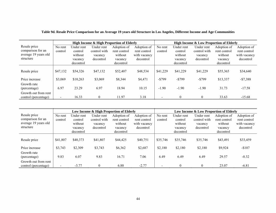
In Table 7c, we show the results for further refined subsamples by both median household

income and proportion of elderly population at the census tract level. When we consider income

and age at the same time, age is a higher order factor than income: both younger communities,

with higher or lower income, enjoy greater benefit from the adoption of rigid rent control than the

older communities. Homeowners in younger communities with higher median household income

are the biggest beneficiaries, while the ones in older communities with lower median household

income experience the lowest benefits. For the newly adopted flexible rent control policies,

homeowners in older communities with higher median household income might be the only

beneficiaries, and all the rest will suffer, especially the ones in younger communities with higher

median income. The future homeowners in the former community will continue benefiting from

rigid rent control but to a lesser extent.

17

Finally, Figure 4b presents the simulated comparison of indexes between units in the

jurisdictions without rent control and units in hypothetical jurisdictions which adopted rigid rent

control in the beginning of 1993. The price index of the latter diverges from the former soon after

the adoption of the policy. In Tables 9a, b, c and d, we report results for an average mobile home

in Los Angeles, we find that if the unit was under a flexible rent control regime before the

original purchase, its real growth rate in price would be 1.7 percentage points less than

comparable units in a market without rent control or units under a rigid rent control regime. In

contrast with an unchanged rent control policy environment, the adoption of rent control between

the first and second transactions leads to a greater and more significant change in prices. More

rigid rent control leads to a growth rate of 13.6 percentage points more than the units in a market

without rent control, or an increase in coach value of $8,081. In contrast, flexible rent control

results in a growth rate 8.8 percentage points lower than the coaches in a market without rent

control, or a loss in value of $1,088.

6. Conclusions

Mobile homes are usually owned by households that pay a periodic rent for use of the land in

a mobile home park (a pad) on which the coach is located. Because mobile homes tend not to be

mobile but rather fixed on the pad on which they are initially located, and since the pads are

rented, economic theory suggests that the imposition of rent control will lead to the capitalization

of future rent savings when a coach is sold. That is, the buyer will not only pay for the coach but

also for the net present value of the expected savings associated with the constrained future pad

rent obligations to the landlord.

Our results support the hypothesis, based on a more extensive and timely data set than had

been employed in similar prior studies in California. Results from our extensive analysis suggest

that higher income groups receive a relatively larger first time rigid rent control premium

(adoption of rigid rent control increases the coach value by 18.6 percent for higher income groups

18

and 12.5 percent for lower income groups, respectively), but also have to face greater losses from

the adoption of flexible rent control (coach value decrease by 11 percent for higher income

groups and 5 percent for lower income groups). Younger owners on average can get about a 24.8

percent premium for adoption of rigid rent control while elderly owners on average benefit from

an 8.6 percent premium which is 18 percentage points lower than the former. On the other hand,

the elderly owners are able to gain from the adoption of flexible rent control policies through a

6.6 percent increase in their coach value, while the younger owners suffer a 3.4 percent decrease.

When we combine the two factors of income and age, higher income younger owners are the

biggest winners from the adoption of rigid rent control which brings them a roughly 34 percent

increase in coach value. In contrast, lower income elderly owners on average benefit the least

from rigid rent control with a 7 percent increase in coach value. Higher income elderly owners

also benefit from rigid rent control with a 16 percent increase in coach values.

We hope to have contributed to the rent control discussion by estimating the size and

incidence of its impacts as well as how they vary with the strictness of the controls. This is a

controversial policy area and we hope that our estimated effects based on a much larger sample

than had heretofore been available as well as the use of more rigorous and detailed methods

enhance the quality of the debate.

19

References

Alston, Richard M., J. R. Kearl, and Michael B. Vaughan, 1992, “Is There a Consensus among Economists in the 1990’s?” American Economic Review, 82, 203-209.

Arnott, Richard, 1995, “Time for Revisionism on Rent Control?” The Journal of Economic Perspectives, 9:1, 99-120.

Arnott, Richard and Masahiro Igarashi, 2000, “Rent Control, Mismatch Costs and Search Efficiency,” Regional Science and Urban Economics, 30, 249-288.

Arnott, Richard, 1998, “Rent Control,” The New Palgrave Dictionary of Economics and the Law, New York: MacMillan and Co.

Bailey, Martin J., Richard F. Muth, and Hugh O. Nourse, 1963, “A Regression Model for Real Estate Price Index Construction,” Journal of the American Statistical Association, 58, 933-942.

Basu, Kaushik and Patrick M. Emerson, 2000, “The Economics and Law of Rent Control,” Economic Journal, 110, 939-962.

Case, Bradford and John M. Quigley, 1991, “The Dynamics of Real Estate Prices,” The Review of Economics and Statistics, 93:1, 50-58.

Case, Karl E. and Robert J. Shiller, 1989, “The Efficiency of the Market for Single Family Homes,” American Economic Review, 79:1, 125-37.

Caudill, Steven B., Richard W. Ault, and Richard P. Saba, 1989, “Efficient Estimation of the Costs of Rent Controls,” The Review of Economics and statistics, 71:1, 154-159.

Clapham, Eric, Peter Englund, John M. Quigley, and Christian L. Redfearn, 2004, “Revisiting the Past: Revision in Repeat Sales and Hedonic Indexes of House Prices”, unpublished working paper.

Deng, Yongheng, John M. Quigley, and Robert Van Order, 2000, “Mortgage Terminations, Heterogeneity and the Exercise of Mortgage Options,” Econometrica, 68, 275-307.

Early, Dirk W. and Edgar O. Olsen, 1998, “Rent Control and Homeless,” Regional Science and Urban Economics, 28, 797-816.

Early, Dirk W., 1999, “Rent Control, Rental Housing Supply, and the Distribution of Tenant Benefits,” Journal or Urban Economics, 48,185-204.

Epple, Dennis, 1998, “Rent Control with Reputation: Theory and Evidence,” Regional Science and Urban Economics, 28, 679-710.

Fallis, George and Lawrence B. Smith, 1984, “Uncontrolled Prices in a Controlled Market: The Case of Rent Control,” The American Economic Review, 74:1, 193-200.

Glaeser, Edwrd L., 1996, “The Social Costs of Rent Control Revisited,” National Bureau of Economic Research Working Paper 5441.

Glaeser, Edward L. and Erzo F.P. Luttmer, 2003, “The Misallocation of Housing Under Rent Control”, The American Economic Review, 93:4, 1027-1046.

Gyourko, Joseph and Linneman, Peter, 1989, “Equity and Efficiency Aspects of Rent Control: An Empirical Study of New York City,” Journal of Urban Economics, 26:1, 54-74.

Harding, John P., Stuart S. Rosenthal, and D.F. Sirmans, 2005, “Depreciation of Housing Capital, Maintenance, and the Gains from Homeownership Estimates From a Repeat Sales Model,” unpublished working paper.

Hill, R. Carter, J.R. Knight, and C.F. Sirmans, 1997, “Estimating Capital Asset Price Indexes,”

20

The Review of Economics and Statistics, 79:2, 226-233.

Hirsch, Werner Z., 1988, “An Inquiry into Effects of Mobile Home Park Rent Control,” Journal of Urban Economics, 24, 212-226.

Hirsch, Werner Z. and Joel G. Hirsch, 1988, “Legal-Economic Analysis of Rent Controls in A Mobile Home Context: Placement Values and Vacancy Decontrol,” UCLA Law Review, 35, 399-467.

Hirsch, Werner Z. and Anthony M. Rufolo, 1999, “The Regulation of Immobile Housing Assets under Divided Ownership,” International Review of Law and Economics, 19, 383-397.

Johnson, D. Gale, 1951, “Rent Control and the Distribution of Income”, The American Economic Review, 41:2, 569-582.

Malpezzi, Stephen, 1998, “Welfare Analysis of Rent Control with Side Payments: A Natural Experiment in Cairo, Egypt,” Regional Science and Urban Economics, 28, 773-795.

Mason, Carl and John M. Quigley, 2004, “The Curious Institution of Mobile Home Rent Control: A Case Study of Mobile Home Parks in California,” unpublished working paper.

Moon, Choon-Geol and Janet G. Stotsky, 1993, “The Effect of Rent Control on Housing Quality Change: A Longitudinal Analysis,” The Journal of Political Economy, 101:6, 1114-1148.

Murray, Michael P., C. Peter Rydell, C. Lance Barnett, Carol E. Hillestad, and Kevin Neels, 1991, “Analyzing Rent Control: The Case of Los Angeles,” Economic Inquiry, 29, 601-625.

Nagy, J., 1997, “Do Vacancy Decontrol Provisions Undo Rent Control?” Journal of Urban Economics, 42, 64-78.

Olsen, Edgar O., 1972, “An Econometric analysis of Rent Control”, The Journal of Political Economy, 80:6, 1081-1100.

Palmquist, Raymond B., 1980, “Alternative Techniques for Developing Real Estate Price Indexes,” The Review of Economics and Statistics, 62: 3, 442-448.

Quigley, John M., 1990, “Does Rent Control Cause Homeless? Taking the Claim Seriously,” Journal of Policy Analysis and Management, 9, 89-93.

Quigley, John M., 2002, “Economic Analysis of Mobile Home Rent Control: The Example of San Rafael, California,” unpublished working paper.

Radford, R. S. 2004, “Why Rent Control Is Still a Regulatory Taking?” unpublished working paper.

Rapaport, Carol, 1992, “Rent Regulation and Housing Market Dynamics,” The American Economic Review, 82:2, 446-451.

Redfearn, Christian L., 2005, “Measure Globally, Aggregate Locally: The Interplay of Housing Market Dynamics and Price Index Construction”, unpublished working paper.

Rubinfeld, Daniel L., 1992, “Regulatory Takings: The Case of Mobile Home Rent Control,” Chicago-Kent Review, 67(3), 923-929.

Tucker, W., 1989, “America’s Homeless: Victims of Rent Control,” Heritage Foundation Backgrounder, 685.

Turner, Bengt and Stephen Malpezzi, 2003, “A Review of Empirical Evidence on the Costs and Benefits of Rent Control,” Swedish Economic Policy Review, 10, 11-56.

US Department of Housing and Urban Development (HUD), 1991, Report to Congress on Rent Control. Office of Policy Development and Research.

Table 1. Definitions of Variables ADDRESS Address CITY Located city COUNTY Located county PARKNAME Mobile home park name PARKID Mobile home park ID MDLYR Model Year MFG Manufacturer TRADE Trade W1/L1 W1/L1 single wide/length W2/L2 W1W2/L1L2 double wide/length W3/L3 W1W2W3/L1L2L3 triple wide/length LEGAL Legal owner SOLD Sold date (year, month, day) ORIG Original sale price (current dollar) CONORIG Original sale price (constant 1996 dollar) RESALE Resale price (current dollar) CONRESALE Resale price (constant 1996 dollar) TYPE Type of the unit (single, double, triple) SIZE Total size of the unit (square footage) WELFARE Proportion of households with public assistance income, census tract MDHHY Median household income (current dollar) census tract OLD Proportion of persons ≥ 65 years old, census tract RENT CONTROL Dummy variable (1: with RC; 0: without RC) DECON Dummy variable (1: RC with vacancy decontrol) NODEC Dummy variable (1: RC without vacancy decontrol)

22

Table 2a. Time Varying Mobile Home Transaction Statistics

Total units traded (square footage, in thousands)

Year All

Rent control group

Rent control with

vacancy decontrol

Rent control without vacancy

decontrol

Percentage of rent control

group (%)

Percentage of rent control with

vacancy decontrol group (%)

Percentage of rent control without


1983 3780.61 549.43 235.73 313.69 14.53 6.24 8.30 1984 4692.13 793.32 403.75 389.57 16.91 8.60 8.30 1985 5338.81 1017.03 537.97 479.05 19.05 10.08 8.97 1986 5660.14 1169.70 659.36 510.34 20.67 11.65 9.02 1987 6159.30 1327.07 755.21 571.87 21.55 12.26 9.28 1988 6908.11 1708.47 955.21 753.26 24.73 13.83 10.90 1989 7668.03 2259.03 1360.25 898.78 29.46 17.74 11.72 1990 6747.48 2230.17 1353.02 877.15 33.05 20.05 13.00 1991 5545.80 1980.36 1212.42 767.93 35.71 21.86 13.85 1992 5588.80 2027.33 1204.14 823.18 36.27 21.55 14.73 1993 6533.61 2840.45 1554.55 1285.91 43.47 23.79 19.68 1994 7749.34 3650.92 1948.21 1702.72 47.11 25.14 21.97 1995 8438.82 4036.33 2013.67 2022.66 47.83 23.86 23.97 1996 7859.52 3427.39 1484.17 1943.22 43.61 18.88 24.72 1997 8421.09 3610.09 1557.90 2052.20 42.87 18.50 24.37 1998 9880.72 4042.02 1668.37 2373.65 40.91 16.89 24.02 1999 10559.00 4098.66 1846.78 2251.88 38.82 17.49 21.33 2000 10742.12 4444.57 1856.43 2588.13 41.38 17.28 24.09 2001 11350.12 4675.10 2134.15 2540.96 41.19 18.80 22.39 2002 11713.24 4629.11 1959.71 2669.40 39.52 16.73 22.79

2003* 3330.66 1339.89 645.71 694.19 40.23 19.39 20.84

* First five months of year 2003.

23

Table 2b. Time Varying Mobile Home Transaction Statistics (Con.)

Total traded value (constant 1996 dollar, in millions)

Year All

Rent control group

Rent control with vacancy

decontrol

Rent control without vacancy decontrol


group (%)





1983 149.15 20.47 8.25 12.22 13.73 5.53 8.19 1984 187.08 30.60 14.57 16.03 16.36 7.79 8.57 1985 214.95 38.27 18.81 19.47 17.81 8.75 9.06 1986 228.32 44.81 23.35 21.46 19.63 10.23 9.40 1987 248.29 51.68 27.23 24.45 20.82 10.97 9.85 1988 282.15 65.51 33.84 31.67 23.22 11.99 11.22 1989 316.37 87.19 48.03 39.16 27.56 15.18 12.38 1990 263.64 81.85 46.54 35.30 31.05 17.65 13.39 1991 187.68 62.05 35.87 26.18 33.06 19.11 13.95 1992 156.79 52.20 29.36 22.84 33.30 18.73 14.57 1993 141.68 60.83 31.11 29.73 42.94 21.96 20.98 1994 143.31 70.03 32.69 37.34 48.87 22.81 26.06 1995 146.08 71.54 30.04 41.50 48.97 20.56 28.41 1996 144.17 65.65 24.06 41.59 45.54 16.69 28.85 1997 172.45 80.86 29.87 50.99 46.89 17.32 29.57 1998 226.68 98.28 33.82 64.46 43.36 14.92 28.44 1999 264.58 105.92 41.79 64.13 40.03 15.79 24.24 2000 330.46 148.97 46.57 102.40 45.08 14.09 30.99 2001 358.56 153.78 56.01 97.77 42.89 15.62 27.27 2002 402.18 166.20 58.98 107.22 41.32 14.67 26.66

2003* 117.17 48.09 20.51 27.58 41.04 17.51 23.54


24

Table 2c. Time Varying Mobile Home Transaction Statistics (Con.)

Number of units transacted

Year All

Rent control group


decontrol



group (%)





1983 3452 455 198 257 13.18 5.74 7.44 1984 4311 671 351 320 15.56 8.14 7.42 1985 4883 848 458 390 17.37 9.38 7.99 1986 5167 974 568 406 18.85 10.99 7.86 1987 5619 1128 652 476 20.07 11.60 8.47 1988 6199 1460 828 632 23.55 13.36 10.20 1989 6763 1918 1197 721 28.36 17.70 10.66 1990 6050 1929 1192 737 31.88 19.70 12.18 1991 5057 1760 1081 679 34.80 21.38 13.43 1992 5150 1862 1113 749 36.16 21.61 14.54 1993 5929 2562 1419 1143 43.21 23.93 19.28 1994 6918 3221 1738 1483 46.56 25.12 21.44 1995 7517 3558 1801 1757 47.33 23.96 23.37 1996 6974 3016 1329 1687 43.25 19.06 24.19 1997 7481 3190 1412 1778 42.64 18.87 23.77 1998 8702 3583 1509 2074 41.17 17.34 23.83 1999 9195 3584 1663 1921 38.98 18.09 20.89 2000 9225 3802 1657 2145 41.21 17.96 23.25 2001 9815 4036 1889 2147 41.12 19.25 21.87 2002 10013 3974 1732 2242 39.69 17.30 22.39

2003* 2801 1133 554 579 40.45 19.78 20.67


25

Table 3. Annual Growth Rates (1984-2002)

Total units traded (square footage) Total traded value (constant 1996 dollar) Number of units transacted

Year All

Rent control group


decontrol

Rent control without vacancy decontrol All

Rent control group


decontrol

Rent control without vacancy decontrol All

Rent control group


decontrol


1984 24.11% 44.39% 71.27% 24.19% 25.43% 49.46% 76.55% 31.17% 24.88% 47.47% 77.27% 24.51% 1985 13.78% 28.20% 33.25% 22.97% 14.89% 25.09% 29.07% 21.47% 13.27% 26.38% 30.48% 21.88% 1986 6.02% 15.01% 22.56% 6.53% 6.22% 17.08% 24.15% 10.25% 5.82% 14.86% 24.02% 4.10% 1987 8.82% 13.45% 14.54% 12.06% 8.75% 15.34% 16.62% 13.95% 8.75% 15.81% 14.79% 17.24% 1988 12.16% 28.74% 26.48% 31.72% 13.64% 26.75% 24.29% 29.50% 10.32% 29.43% 26.99% 32.77% 1989 11.00% 32.23% 42.40% 19.32% 12.13% 33.10% 41.92% 23.66% 9.10% 31.37% 44.57% 14.08% 1990 -12.01% -1.28% -0.53% -2.41% -16.67% -6.13% -3.09% -9.85% -10.54% 0.57% -0.42% 2.22% 1991 -17.81% -11.20% -10.39% -12.45% -28.81% -24.19% -22.93% -25.84% -16.41% -8.76% -9.31% -7.87% 1992 0.78% 2.37% -0.68% 7.20% -16.46% -15.87% -18.15% -12.74% 1.84% 5.80% 2.96% 10.31% 1993 16.91% 40.11% 29.10% 56.21% -9.64% 16.53% 5.94% 30.13% 15.13% 37.59% 27.49% 52.60% 1994 18.61% 28.53% 25.32% 32.41% 1.15% 15.13% 5.10% 25.61% 16.68% 25.72% 22.48% 29.75% 1995 8.90% 10.56% 3.36% 18.79% 1.93% 2.15% -8.12% 11.14% 8.66% 10.46% 3.62% 18.48% 1996 -6.86% -15.09% -26.30% -3.93% -1.31% -8.23% -19.90% 0.22% -7.22% -15.23% -26.21% -3.98% 1997 7.15% 5.33% 4.97% 5.61% 19.61% 23.17% 24.15% 22.60% 7.27% 5.77% 6.25% 5.39% 1998 17.33% 11.96% 7.09% 15.66% 31.45% 21.54% 13.19% 26.43% 16.32% 12.32% 6.87% 16.65% 1999 6.86% 1.40% 10.69% -5.13% 16.72% 7.77% 23.57% -0.52% 5.67% 0.03% 10.21% -7.38% 2000 1.73% 8.44% 0.52% 14.93% 24.90% 40.64% 11.44% 59.67% 0.33% 6.08% -0.36% 11.66% 2001 5.66% 5.19% 14.96% -1.82% 8.51% 3.23% 20.28% -4.52% 6.40% 6.15% 14.00% 0.09% 2002 3.20% -0.98% -8.17% 5.05% 12.16% 8.07% 5.30% 9.66% 2.02% -1.54% -8.31% 4.42%

Average annual growth

rate

6.65% 13.02% 13.71% 13.00% 6.56% 13.19% 13.13% 13.79% 6.22% 13.17% 14.07% 13.00%

26

Figure 1a. Total Traded Square Footage (in thousands)

0

2,000

4,000

6,000

8,000

10,000

12,000

14,000

1983 1984 1985 1986 1987 1988 1989 1990 1991 1992 1993 1994 1995 1996 1997 1998 1999 2000 2001 2002

Without rent control Rent control with vacancy decontrol Rent control w/o vacancy decontrol

27

Figure 1b. Total Traded Value (constant $, base=1996) (in millions)

0

50

100

150

200

250

300

350

400

450

1983 1984 1985 1986 1987 1988 1989 1990 1991 1992 1993 1994 1995 1996 1997 1998 1999 2000 2001 2002


28

Figure 1c. Number of Transactions

0

2,000

4,000

6,000

8,000

10,000

12,000

1983 1984 1985 1986 1987 1988 1989 1990 1991 1992 1993 1994 1995 1996 1997 1998 1999 2000 2001 2002


29

Table 4. Descriptive Statistics – means and standard deviations of continuous covariates

All Los

Angeles Orange Riverside San

Bernardino San

Diego Santa Clara Ventura

Original price (constant 1996 dollar) 40,775 40,696 45,362 39,691 36,940 38,102 46,410 38,699 (21150) (22183) (21313) (20029) (18324) (19407) (25154) (18691) Resale price (constant 1996 dollar) 34,118 33,207 38,982 28,567 22,085 30,925 54,441 42,687 (26201) (24331) (26981) (25116) (17834) (22767) (31546) (28392) Median household income (constant 1996 dollar) 43,274 46,923 47,193 33,149 36,650 39,991 52,492 48,194 (13524) (14011) (12135) (9862) (11097) (10462) (15100) (11262) Proportion of households with public assistance income 0.067 0.070 0.052 0.086 0.090 0.059 0.057 0.050 (0.047) (0.046) (0.039) (0.040) (0.053) (0.045) (0.044) (0.033) Proportion of persons ≥ 65 years old 0.132 0.103 0.117 0.244 0.115 0.151 0.114 0.122 (0.094) (0.055) (0.088) (0.160) (0.067) (0.083) (0.079) (0.052) Unit's size (sq. ft.) 1,127 1,094 1,199 1,160 1,093 1,103 1,158 1,113 (396) (411) (370) (422) (383) (389) (406) (376) Unit's age 19.23 19.10 19.28 16.01 19.09 20.75 18.82 20.85 (9.15) (9.39) (9.15) (8.51) (9.24) (9.07) (8.55) (8.61) Sample size 137,221 31,404 23,934 12,912 20,827 28,551 13,423 6,170 Note: Standard deviations are in parenthesis.

30

Table 5. Descriptive Statistics – frequencies of categorical covariates

All Los

Angeles Orange Riverside San

Bernardino San Diego Santa Clara Ventura

Single 35,787 9,157 3,532 3,513 6,741 7,820 3,325 1,699 (26.1) (29.2) (14.8) (27.2) (32.4) (27.4) (24.8) (27.5) Double 94,110 20,394 18,997 8,338 13,265 19,457 9,412 4,247 (68.6) (64.9) (79.4) (64.6) (63.7) (68.1) (70.1) (68.8) Triple 7,324 1,853 1,405 1,061 821 1,274 686 224 (5.3) (5.9) (5.9) (8.2) (3.9) (4.5) (5.1) (3.6) Rent Control 48,664 8,828 1,092 7,865 8,959 10,871 5,948 5,101 (35.5) (28.1) (4.6) (60.9) (43.0) (38.1) (44.3) (82.7) Rent control with vacancy decontrol 24,341 7,035 1 5,720 3,401 4,745 252 3,187 (17.7) (22.4) (0.0) (44.3) (16.3) (16.6) (1.9) (51.7) Rent control without vacancy decontrol 24,323 1,793 1,091 2,145 5,558 6,126 5,696 1,914 (17.7) (5.7) (4.6) (16.6) (26.7) (21.5) (42.4) (31.0)

20,980 5,926 1 4,862 2,833 4,399 228 2,731 Adoption of rent control with vacancy decontrol (15.3) (18.9) (0.0) (37.7) (13.6) (15.4) (1.7) (44.3)

21,723 1,415 1,041 1,942 5,148 5,445 5,063 1,669 Adoption of rent control without vacancy decontrol (15.8) (4.5) (4.3) (15.0) (24.7) (19.1) (37.7) (27.1)

Sample size 137,221 31,404 23,934 12,912 20,827 28,551 13,423 6,170 Note: Percentages to corresponding full or county samples are in parenthesis.

31

Figure 2. Logarithm of Price Growth Rate by Sub-Groups

These figures present the box plot of the logarithm of price growth rates by various sub-groups. The boxes contain the middle 50% of the data. The upper edges of the boxes indicate the 75th percentile of the data set, and the lower edges indicate the 25th percentile. The lines in the boxes indicate the median value of the data. The ends of the vertical lines indicate the minimum and maximum data values. The logarithm of price growth rate is defined as:

ln( )t

t

P

Pτ+ , where ( )ln i is natural logarithm function, tP τ+ is the resale price after τ periods since the original sale

at t , tP is the original sales price at t .

Figure 2a. Logarithm of Price Growth Rate by County

32

Figure 2b. Logarithm of Price Growth Rate by Coach Structure

Figure 2c. Logarithm of Price Growth Rate by Rent Control Regime

33

Table 6. GLS Estimates for Rent Control Impact on Mobile Home Price

The table reports rent control impacts on mobile home prices. We estimate the rent control impact by decomposing the capitalization of rent control premium from a repeated-sales mobile home price index model specified in equations (9) and (10) using a three-stage GLS estimation approach. In the first stage, we use OLS to estimate the following mobile home price index model which decomposes the rent control premium capitalization from the mobile home price appreciation: ( )' 'ln( ) ' ( )t

t tt

P D Z RC RCPτ

τγ θ δ μ τ++= + + − + , where ( )ln i is

natural logarithm function, tP τ+ is the resale price after τ periods since the original sale at t , tP is the original sales price at t , D is a repeated-sales transaction vector composed of -1, 0 and 1; RC is a vector of indicator variables to capture the rent control premium capitalization; Z is a vector of hedonic characteristics capturing the location effect (measured by county), and coach structure characteristics, such as single, double, or triple-width, size, and neighborhood quality, etc., and μ is the normally distributed error term with a diffusion variance varying by the time span between two transactions. In the second stage, we estimate a diffusion process of the mobile home price index by regressing the square term of residuals, 2ε , collected from the first stage OLS regression on a quadratic

function of time span between the two sales, such that, ( ) 221 2

ε τ β τ β τ ω= + + , where τ is the duration between original sale and

resale (measured in quarters), and ω is a normally distributed error term. In the third stage we re-estimate the mobile home price index model using a GLS estimation approach weighted by the square root of the estimated diffusion variance, ( )ε̂ τ , obtained from the second stage. Fore readability, the estimated mobile home price indices are not reported in the table.

Impact of Rent Control Impact of Rent Control together with Other Effects (1) (2) (3) Orange County -0.04 -0.04 (-8.79) (-8.38) Riverside -0.28 -0.27 (-45.92) (-45.91) San Bernardino -0.30 -0.29 (-55.88) (-55.03) San Diego 0.31 -0.03 (50.24) (-6.47) Santa Clara -0.03 0.33 (-6.17) (53.87) Ventura 0.37 0.36 (42.13) (41.59) Double 0.19 0.19 (30.34) (30.39) Triple 0.26 0.27 (21.25) (21.46) Size 1.63E-05 1.67E-05 (2.47) (2.54)

-1.39 -1.34 (-39.57) (-38.18)

Under rent control without vacancy decontrol 0.01 0.01 (1.44) (1.10)

-0.02 -0.02 Under rent control with vacancy decontrol (-1.85) (-1.88) Adoption of rent control without vacancy decontrol 0.15 0.12 (28.77) (23.22)

0.015 Adoption of rent control without vacancy decontrol × number of months years under rent control (30.06)

-0.11 -0.09 -0.08 Adoption of rent control with vacancy decontrol (-20.70) (-16.57) (-15.76) R square 0.412 0.496 0.498 Sample size 137,221 137,221 137,221

34

Figure 3. Logarithm of Price Growth Rate by Income and Age Sub-Groups

These figures present the box plot of the logarithm of price growth rates by various sub-groups. The boxes contain the middle 50 percent of the data. The upper edges of the boxes indicate the 75th percentile of the data set, and the lower edges indicate the 25th percentile. The lines in the boxes indicate the median value of the data. The ends of the vertical lines indicate the minimum and maximum data values. The logarithm of price growth rate is defined as: ln( )t

t

P

Pτ+ , where ( )ln i is natural logarithm function, tP τ+

is the resale price after τ periods since the original sale at t , tP is the original sales price at t .

Figure 3a. Logarithm of Price Growth Rate by Income Group

Figure 3b. Logarithm of Price Growth Rate by Age Group

35

Table 7. GLS Estimates for Logarithm of Price Growth Rate, by Subgroups

The table reports rent control impacts on mobile home prices. We estimate the rent control impact by decomposing the capitalization of rent control premium from a repeated-sales mobile home price index model specified in equations (9) and (10) using a three-stage GLS estimation approach. In the first stage, we use OLS to estimate the following mobile home price index model which decomposes the rent control premium capitalization from the mobile home price appreciation:

( )' 'ln( ) ' ( )tt t

t

P D Z RC RCPτ

τγ θ δ μ τ++= + + − + , where ( )ln i is natural logarithm function, tP τ+ is the resale price after τ

periods since the original sale at t , tP is the original sales price at t , D is a repeated-sales transaction vector composed of -1, 0 and 1; RC is a vector of indicator variables to capture the rent control premium capitalization; Z is a vector of hedonic characteristics capturing the location effect (measured by county), and coach structure characteristics, such as single, double, or triple-width, size, and neighborhood quality, etc., and μ is the normally distributed error term with a diffusion variance varying by the time span between two transactions. In the second stage, we estimate a diffusion process of the mobile home price index by regressing the square term of residuals, 2ε , collected from the first stage OLS regression on a quadratic function of time span between the two sales, such that, ( )2 2

1 2ε τ β τ β τ ω= + + , where τ is the duration between original sale and resale (measured in quarters), and ω is a normally distributed error term. In the third stage we re-estimate the mobile home price index model using a GLS estimation approach weighted by the square root of the estimated diffusion variance, ( )ε̂ τ , obtained from the second stage. Fore readability, the estimated mobile home price indices are not reported in the table.

36

Table 7a. GLS Estimates for Logarithm of Price Growth Rate, by Census Tract Household Income

Higher Median Household

Income Lower Median Household

Income Orange County 0.04 -0.07 (4.49) (-9.53) Riverside -0.17 -0.34 (-18.21) (-39.15) San Bernardino -0.23 -0.35 (-29.81) (-44.49) San Diego 0.17 0.36 (13.57) (42.96) Santa Clara -0.061 -0.004 (-9.10) (-0.58) Ventura 0.37 0.37 (22.29) (33.58) Double 0.17 0.20 (16.65) (24.68) Triple 0.25 0.27 (13.41) (15.55) Size -1.22E-05 4.10E-05 (-1.23) (4.46)

-2.10 -1.00 Proportion of households with public assistance income (-26.47) (-22.94) 0.070 -0.014 Under rent control without vacancy decontrol (4.90) (-1.04) -0.02 0.01 Under rent control with vacancy decontrol

(-1.95) (0.44) 0.16 0.12 Adoption of rent control without vacancy decontrol

(18.40) (18.21) -0.11 -0.05 Adoption of rent control with vacancy decontrol

(-14.12) (-7.40) R square 0.44 0.54 Sample size 52,921 84,300

37

Table 7b. GLS Estimates for Logarithm of Price Growth Rate, by Census Tract Proportion of Elderly Population

Higher Proportion of Elderly Population

Lower Proportion of Elderly Population

Orange County -0.05 -0.03 (-6.50) (-4.75) Riverside -0.36 -0.21 (-40.69) (-25.65) San Bernardino -0.41 -0.19 (-54.09) (-25.75) San Diego 0.32 0.31 (36.98) (33.88) Santa Clara -0.08 0.03 (-11.78) (3.94) Ventura 0.33 0.41 (26.63) (33.51) Double 0.17 0.21 (18.40) (24.56) Triple 0.23 0.26 (13.26) (14.78) Size 4.99E-05 -2.63E-05 (5.21) (-2.96)

-1.13 -1.21 Proportion of households with public assistance income (-19.42) (-27.02)

0.06 -0.03 Under rent control without vacancy decontrol (4.29) (-2.51) 0.02 -0.03 Under rent control with vacancy decontrol

(1.73) (-2.54) 0.08 0.21 Adoption of rent control without vacancy decontrol

(11.50) (24.80) -0.02 -0.14 Adoption of rent control with vacancy decontrol

(-2.90) (-17.16) R square 0.48 0.52 Sample size 69,547 67,674

38

Table 7c. GLS Estimates for Logarithm of Price Growth Rate, by Census Tract Median Household Income and Proportion of

Elderly Population

High Income & High Proportion of Elderly

High Income & Low Proportion of Elderly

Low Income & High Proportion of Elderly

Low Income & Low Proportion of Elderly

Orange County 0.08 0.01 -0.02 -0.10 (6.96) (1.01) (-1.98) (-10.25) Riverside -0.21 -0.11 -0.32 -0.35 (-9.93) (-10.58) (-27.73) (-27.11) San Bernardino -0.47 -0.11 -0.35 -0.34 (-33.53) (-11.69) (-32.54) (-27.66) San Diego 0.33 0.15 0.40 0.31 (15.24) (9.68) (34.83) (24.44) Santa Clara -0.10 -0.02 0.01 0.01 (-9.92) (-1.91) (0.78) (1.14) Ventura 0.34 0.40 0.42 0.33 (10.94) (20.03) (28.25) (18.97) Double 0.16 0.17 0.19 0.22 (9.70) (13.29) (16.54) (18.68) Triple 0.26 0.18 0.26 0.25 (9.18) (7.68) (11.60) (9.51) Size -1.58E-05 -1.24E-05 4.04E-05 2.85E-05 (-1.01) (-0.99) (3.19) (2.12)

-0.99 -2.09 -0.88 -0.97 Proportion of households with public assistance income (-6.62) (-22.27) (-12.72) (-16.14)

0.15 -0.01 -0.04 0.02 Under rent control without vacancy decontrol (6.64) (-0.34) (-1.98) (1.11)

-0.011 -0.003 0.022 0.009 Under rent control with vacancy decontrol (-0.43) (-0.20) (1.30) (0.57)

0.11 0.26 0.06 0.22 Adoption of rent control without vacancy decontrol (8.49) (19.93) (7.82) (19.23)

0.031 -0.148 -0.03 -0.07 Adoption of rent control with vacancy decontrol (2.53) (-14.08) (-2.89) (-6.06)

R square 0.41 0.49 0.53 0.55 Sample size 24,826 28,095 44,721 39,579

39

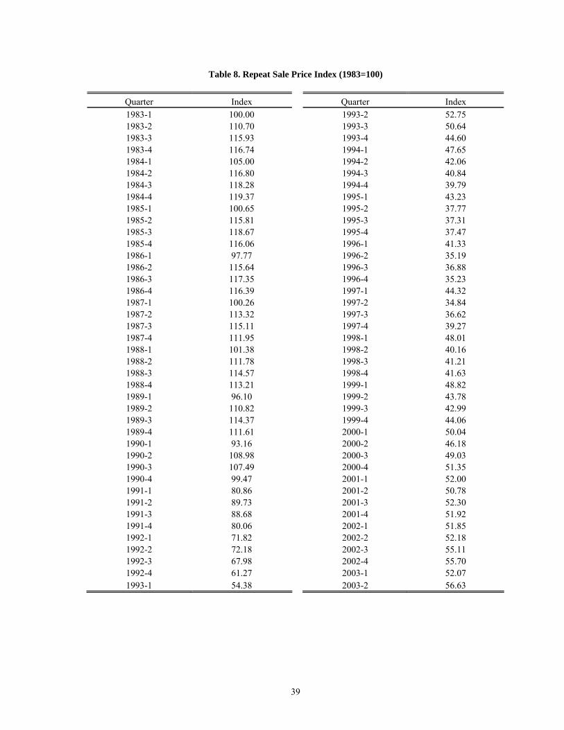
Table 8. Repeat Sale Price Index (1983=100)

Quarter Index Quarter Index 1983-1 100.00 1993-2 52.75 1983-2 110.70 1993-3 50.64 1983-3 115.93 1993-4 44.60 1983-4 116.74 1994-1 47.65 1984-1 105.00 1994-2 42.06 1984-2 116.80 1994-3 40.84 1984-3 118.28 1994-4 39.79 1984-4 119.37 1995-1 43.23 1985-1 100.65 1995-2 37.77 1985-2 115.81 1995-3 37.31 1985-3 118.67 1995-4 37.47 1985-4 116.06 1996-1 41.33 1986-1 97.77 1996-2 35.19 1986-2 115.64 1996-3 36.88 1986-3 117.35 1996-4 35.23 1986-4 116.39 1997-1 44.32 1987-1 100.26 1997-2 34.84 1987-2 113.32 1997-3 36.62 1987-3 115.11 1997-4 39.27 1987-4 111.95 1998-1 48.01 1988-1 101.38 1998-2 40.16 1988-2 111.78 1998-3 41.21 1988-3 114.57 1998-4 41.63 1988-4 113.21 1999-1 48.82 1989-1 96.10 1999-2 43.78 1989-2 110.82 1999-3 42.99 1989-3 114.37 1999-4 44.06 1989-4 111.61 2000-1 50.04 1990-1 93.16 2000-2 46.18 1990-2 108.98 2000-3 49.03 1990-3 107.49 2000-4 51.35 1990-4 99.47 2001-1 52.00 1991-1 80.86 2001-2 50.78 1991-2 89.73 2001-3 52.30 1991-3 88.68 2001-4 51.92 1991-4 80.06 2002-1 51.85 1992-1 71.82 2002-2 52.18 1992-2 72.18 2002-3 55.11 1992-3 67.98 2002-4 55.70 1992-4 61.27 2003-1 52.07 1993-1 54.38 2003-2 56.63

40

Figure 4a. Full Sample Index

0

20

40

60

80

100

120

140

1983

0119

8304

1984

0319

8502

1986

0119

8604

1987

0319

8802

1989

0119

8904

1990

0319

9102

1992

0119

9204

1993

0319

9402

1995

0119

9504

1996

0319

9702

1998

0119

9804

1999

0320

0002

2001

0120

0104

2002

0320

0302

41

Figure 4b. Comparison in Indexes: No Rent Control vs. Change in Rent Control Policy (Adoption of Rent Control without Decontrol)

30

35

40

45

50

55

60

65

70

75

1992

0119

9203

1993

0119

9303

1994

0119

9403

1995

0119

9503

1996

0119

9603

1997

0119

9703

1998

0119

9803

1999

0119

9903

2000

0120

0003

2001

0120

0103

2002

0120

0203

2003

01

Quarter

Adoption of rent control without decontrol No rent control

Adoption of rent control without decontrol

42

Table 9. Resale Price Comparison for an Average 19 years old Structure in Los Angeles The following Tables present the estimated resale prices for the average 19 years old mobile home units in each subgroup in Los Angeles County, under different rent control regimes. The average unit is defined as the one with average structure (double, triple), in census tract with average proportion of households with public assistance income, etc. By using the average units' characteristics and the parameters estimated in Table 7, we can simulate the resale prices as presented here.

Table 9a. Resale Price Comparison for an Average 19 years old Structure in Los Angeles Rent Control Regime

Resale price comparison for an average 19 years old structure

No rent control

Under rent control without vacancy decontrol

Under rent control with

vacancy decontrol

Adoption of rent control

without vacancy decontrol


with vacancy decontrol

Resale price $43,263 $43,263 $42,588 $48,824 $39,656 Price increase $2,519 $2,519 $1,845 $8,081 -$1,088 Growth rate (percentage) 6.18 6.18 4.53 19.83 -2.67 Growth out from rent control (percentage) - 0 -1.66 13.65 -8.85

43

Table 9b. Resale Price Comparison for an Average 19 years old Structure in Los Angeles, Different Income Communities

High Median Household Income Low Median Household Income Resale price comparison for an average 19 years old structure

No rent control

Under rent control without vacancy

decontrol


vacancy decontrol


without vacancy

decontrol



No rent control


decontrol


vacancy decontrol





Resale price $43,500 $46,760 $42,427 $51,538 $38,731 $38,237 $38,237 $38,418 $42,664 $36,406 Price increase $366 $3,625 -$707 $8,403 -$4,403 $2,744 $2,744 $2,926 $7,172 $914 Growth rate (percentage) 0.85 8.40 -1.64 19.48 -10.21 7.73 7.73 8.24 20.21 2.57 Growth out from rent control (percentage) - 7.56 -2.49 18.63 -11.05 - 0 0.51 12.47 -5.16

Table 9c. Resale Price Comparison for an Average 19 years old Structure in Los Angeles, Different Age Communities

High Proportion of Elderly Population Low Proportion of Elderly Population Resale price comparison for an average 19 years old structure

No rent control



vacancy decontrol





No rent control



vacancy decontrol





Resale price $47,383 $50,199 $48,503 $51,030 $46,435 $39,892 $38,574 $38,796 $49,560 $34,617 Price increase $4,903 $7,720 $6,024 $8,550 $3,956 $938 -$381 -$159 $10,605 -$4,338 Growth rate (percentage) 11.54 18.17 14.18 20.13 9.31 2.41 -0.98 -0.41 27.22 -11.14 Growth out from rent control (percentage) - 6.63 2.64 8.59 -2.23 - -3.38 -2.82 24.82 -13.54

44

Table 9d. Resale Price Comparison for an Average 19 years old Structure in Los Angeles, Different Income and Age Communities

High Income & High Proportion of Elderly High Income & Low Proportion of Elderly

Resale price comparison for an average 19 years old structure

No rent control



vacancy decontrol


without vacancy

decontrol



No rent control


decontrol


vacancy decontrol


without vacancy

decontrol



Resale price $47,132 $54,326 $47,132 $52,407 $48,534 $41,229 $41,229 $41,229 $55,365 $34,640 Price increase $3,069 $10,263 $3,069 $8,344 $4,471 -$799 -$799 -$799 $13,337 -$7,388 Growth rate (percentage) 6.97 23.29 6.97 18.94 10.15 -1.90 -1.90 -1.90 31.73 -17.58 Growth out from rent control (percentage) - 16.33 0 11.97 3.18 - 0 0 33.63 -15.68

Low Income & High Proportion of Elderly Low Income & Low Proportion of Elderly Resale price comparison for an average 19 years old structure

No rent control



vacancy decontrol


without vacancy

decontrol



No rent control


decontrol


vacancy decontrol


without vacancy

decontrol



Resale price $41,807 $40,373 $41,807 $44,425 $40,751 $35,746 $35,746 $35,746 $43,491 $33,459 Price increase $3,743 $2,309 $3,743 $6,362 $2,687 $2,180 $2,180 $2,180 $9,924 -$107 Growth rate (percentage) 9.83 6.07 9.83 16.71 7.06 6.49 6.49 6.49 29.57 -0.32 Growth out from rent control (percentage) - -3.77 0 6.88 -2.77 - 0 0 23.07 -6.81

45

Figure 5. Simulation Results: Resale Price Comparison for Los Angeles County

The following figures present the estimated resale prices for the average 19 years old mobile home units in each subgroup in Los Angeles County, under different rent control regimes. The average unit is defined as the one with average structure (double, triple), in census tract with average proportion of households with public assistance income, etc.

Figure 5a. Resale Price Comparison

$30,000

$32,000

$34,000

$36,000

$38,000

$40,000

$42,000

$44,000

$46,000

$48,000

$50,000

No rent control Under rent control withoutvacancy decontrol

Under rent control withvacancy decontrol

Adoption of rent controlwithout vacancy decontrol

Adoption of rent control withvacancy decontrol

46

Figure 5b. Resale Price Comparison-Median Household Income

$30,000

$35,000

$40,000

$45,000

$50,000

$55,000

No rentcontrol

Under rentcontrolwithoutvacancy

decontrol

Under rentcontrol with

vacancydecontrol

Adoption ofrent control

withoutvacancy

decontrol


with vacancydecontrol

No rentcontrol


decontrol


vacancydecontrol


withoutvacancy

decontrol



High Median Household Income Low Median Household Income

47

Figure 5c. Resale Price Comparison-Age Community

$30,000

$35,000

$40,000

$45,000

$50,000

$55,000

No rentcontrol


decontrol


vacancydecontrol


withoutvacancy

decontrol



No rentcontrol


decontrol


vacancydecontrol


withoutvacancy

decontrol



High Proportion of Elderly Population Low Proportion of Elderly Population

48

Figure 5d. Resale Price Comparison-Median Household Income and Elderly Proportion

$30,000

$35,000

$40,000

$45,000

$50,000

$55,000

$60,000

No

rent

con

trol

Und

er re

nt c

ontro

l with

out v

acan

cy d

econ

trol

Und

er re

nt c

ontro

l with

vac

ancy

dec

ontro

l

Ado

ptio

n of

rent

con

trol w

ithou

t vac

ancy

deco

ntro

l

Ado

ptio

n of

rent

con

trol w

ith v

acan

cy d

econ

trol

No

rent

con

trol

Und

er re

nt c

ontro

l with

out v

acan

cy d

econ

trol

Und

er re

nt c

ontro

l with

vac

ancy

dec

ontro

l

Ado

ptio

n of

rent

con

trol w

ithou

t vac

ancy

deco

ntro

l

Ado

ptio

n of

rent

con

trol w

ith v

acan

cy d

econ

trol

No

rent

con

trol

Und

er re

nt c

ontro

l with

out v

acan

cy d

econ

trol

Und

er re

nt c

ontro

l with

vac

ancy

dec

ontro

l

Ado

ptio

n of

rent

con

trol w

ithou

t vac

ancy

deco

ntro

l

Ado

ptio

n of

rent

con

trol w

ith v

acan

cy d

econ

trol

No

rent

con

trol

Und

er re

nt c

ontro

l with

out v

acan

cy d

econ

trol

Und

er re

nt c

ontro

l with

vac

ancy

dec

ontro

l

Ado

ptio

n of

rent

con

trol w

ithou

t vac

ancy

deco

ntro

l

Ado

ptio

n of

rent

con

trol w

ith v

acan

cy d

econ

trol

High Income & High Proportion ofElderly

High Income & Low Proportion ofElderly

Low Income & High Proportion ofElderly

Low Income & Low Proportionof Elderly

Documents

An Examination of the Impact of Rent Control on Mobile Home