An Evaluation of Possible Next-Generation High-Temperature ... · National Solar Thermal Test Facility (NSTTF) Sandia National Laboratories P.O. Box 5800 Albuquerque, New Mexico 87185-1127

SANDIA REPORT SAND2011-9320 Unlimited Release Printed December 2011

An Evaluation of Possible Next-Generation High-Temperature Molten-Salt Power Towers Gregory J. Kolb Prepared by Sandia National Laboratories Albuquerque, New Mexico 87185 and Livermore, California 94550 Sandia National Laboratories is a multi-program laboratory managed and operated by Sandia Corporation, a wholly owned subsidiary of Lockheed Martin Corporation, for the U.S. Department of Energy’s National Nuclear Security Administration under contract DE-AC04-94AL85000. Approved for public release; further dissemination unlimited.

2

Issued by Sandia National Laboratories, operated for the United States Department of Energy by Sandia Corporation. NOTICE: This report was prepared as an account of work sponsored by an agency of the United States Government. Neither the United States Government, nor any agency thereof, nor any of their employees, nor any of their contractors, subcontractors, or their employees, make any warranty, express or implied, or assume any legal liability or responsibility for the accuracy, completeness, or usefulness of any information, apparatus, product, or process disclosed, or represent that its use would not infringe privately owned rights. Reference herein to any specific commercial product, process, or service by trade name, trademark, manufacturer, or otherwise, does not necessarily constitute or imply its endorsement, recommendation, or favoring by the United States Government, any agency thereof, or any of their contractors or subcontractors. The views and opinions expressed herein do not necessarily state or reflect those of the United States Government, any agency thereof, or any of their contractors. Printed in the United States of America. This report has been reproduced directly from the best available copy. Available to DOE and DOE contractors from U.S. Department of Energy Office of Scientific and Technical Information P.O. Box 62 Oak Ridge, TN 37831 Telephone: (865) 576-8401 Facsimile: (865) 576-5728 E-Mail: [email protected] Online ordering: http://www.osti.gov/bridge Available to the public from U.S. Department of Commerce National Technical Information Service 5285 Port Royal Rd. Springfield, VA 22161 Telephone: (800) 553-6847 Facsimile: (703) 605-6900 E-Mail: [email protected] Online order: http://www.ntis.gov/help/ordermethods.asp?loc=7-4-0#online

mailto:[email protected]

http://www.osti.gov/bridge

mailto:[email protected]

http://www.ntis.gov/help/ordermethods.asp?loc=7-4-0#online

3

SAND2011-9320 Unlimited Release

Printed December 2011

An Evaluation of Possible Next-Generation High Temperature Molten-Salt Power Towers

Gregory J. Kolb National Solar Thermal Test Facility (NSTTF)

Sandia National Laboratories P.O. Box 5800

Albuquerque, New Mexico 87185-1127

Abstract

Since completion of the Solar Two molten-salt power tower demonstration in 1999, the solar industry has been developing initial commercial-scale projects that are 3 to 14 times larger. Like Solar Two, these initial plants will power subcritical steam-Rankine cycles using molten salt with a temperature of 565 °C. The main question explored in this study is whether there is significant economic benefit to develop future molten-salt plants that operate at a higher receiver outlet temperature. Higher temperatures would allow the use of supercritical steam cycles that achieve an improved efficiency relative to today’s subcritical cycle (~50% versus ~42%). The levelized cost of electricity (LCOE) of a 565 °C subcritical baseline plant was compared with possible future-generation plants that operate at 600 or 650 °C. The analysis suggests that ~8% reduction in LCOE can be expected by raising salt temperature to 650 °C. However, most of that benefit can be achieved by raising the temperature to only 600 °C. Several other important insights regarding possible next-generation power towers were also drawn: (1) the evaluation of receiver-tube materials that are capable of higher fluxes and temperatures, (2) suggested plant reliability improvements based on a detailed evaluation of the Solar Two experience, and (3) a thorough evaluation of analysis uncertainties.

4

ACKNOWLEDGMENTS I would like to thank several of my colleagues who provided support to this work and kept me from “reinventing the wheel,” which I hate to do. Bruce Kelly (Abengoa) gave me an initial set of GateCycle power-block models he developed under another recent Department of Energy project. He was always there to answer my persistent questions to allow me to successfully modify the models to meet the needs of the current study. Mike Wagner (National Renewable Energy Laboratory) developed a detailed multi-node receiver thermal model as part of his recent Master’s Thesis. I decided to use Mike’s model, rather than the one developed during the Solar Two project, to avoid recoding the defunct Solar Two model and because Mike’s model is similar to the one now in the System Advisor Model (SAM). Mike also made several modifications to this model to meet the needs of the current study. I obtained an algorithm developed by Siri Khalsa (Sandia National Laboratories [SNL] contractor) for another project that allowed me to quickly run SOLERGY the hundreds of times necessary to perform the uncertainty analysis. He is a mathematical genius who wants to use his analytical skills to save lives! He left SNL in the summer of 2011 and is now in medical school. Cliff Ho (SNL) ran the Latin-Hypercube sampling and stepwise-rank-regression software for me to support the uncertainty analysis. The last time I used this software was in 1992 and I did not want to relearn it, especially when I have an expert right down the hall. Finally, Bob Bradshaw (SNL, now retired) provided a concise table of expected corrosion rates for proposed receiver tube materials when exposed to molten salt. This avoided my review (and likely misinterpretation) of experimental results he has published in countless reports over the last 30 years. He was also willing to use his expert judgment to “fill in the blanks” when data were lacking.

5

CONTENTS

Chapter 1 Introduction ...................................................................................................................11 1.1 Overview of Molten-Salt Power Towers ......................................................................... 11 1.2 Overview of Study Tasks ................................................................................................ 14 1.3 Overview of Methodology and Data ............................................................................... 15

Chapter 2 Plant Design Definition .................................................................................................19 2.1 Plant Optical Designs ...................................................................................................... 19 2.2 Receiver Designs ............................................................................................................. 23 2.3 Salt Steam Generator Design .......................................................................................... 33 2.4 Balance of Plant ............................................................................................................... 38

Chapter 3 Performance Analysis ...................................................................................................47 3.1 Overview of the SOLERGY Computer Code ................................................................. 47 3.2 Development of SOLERGY Input Parameters ............................................................... 48 3.3 SOLERGY Analysis Results ........................................................................................... 66

Chapter 4 Reliability Analysis .......................................................................................................75 4.1 Overview of Pro-Opta Reliability Analysis Software ..................................................... 75 4.2 Validation of Pro-Opta with Solar One Data .................................................................. 75 4.3 Reliability Analysis of a Molten-Salt Power Tower ....................................................... 77

4.3.1 Logic Model Development .................................................................................. 77 4.3.2 Reliability Data Base ........................................................................................... 79 4.3.3 Plant Availability Prediction ............................................................................... 82 4.3.4 Plant Availability Improvement Opportunities ................................................... 83

Chapter 5 Levelized-Energy Cost Calculations .............................................................................89

Chapter 6 Uncertainty Analysis .....................................................................................................93 6.1 Goal and Philosophy ....................................................................................................... 93 6.2 Methodology ................................................................................................................... 93 6.3 Results ........................................................................................................................... 101

Chapter 7 Conclusions .................................................................................................................103

References ....................................................................................................................................107

APPENDIX A – Analysis of Operating Hours and Failures at Solar Two from January 14, 1998, to April 8, 1999 .............................................................................................................113

6

FIGURES Figure 1. Flow schematic of a molten-salt central receiver system. .............................................12 Figure 2. In the Solar Two receiver, molten salt flowed through 20-mm tubes arranged

within 24 panels. There were two flow paths, each containing 12 panels. .............................13 Figure 3. Study tasks. ....................................................................................................................14 Figure 4. The 95-m2 Generation 3 heliostat built by ATS in the 1980s is similar to the

default heliostat described in the DELSOL User’s Manual [10]. ............................................20 Figure 5. Receiver system schematic. ...........................................................................................23 Figure 6. Low-cycle fatigue strength for I-800, I-800H, and I-800HT alloys at temperatures

from 70 oF to 1400 oF [26]. Curves appear to have short hold times. Black squares are data from four tests of I800 reported in Reference 33 given 5-hour hold times. .....................26

Figure 7. Number of strain cycles. ................................................................................................26 Figure 8. Allowable strain range. ..................................................................................................28 Figure 9. Receiver tube heated by uniform solar flux. .................................................................28 Figure 10. Receiver temperatures at equinox noon, 565 oC salt outlet temperature. ....................34 Figure 11. Receiver temperatures at equinox noon, 600 oC salt outlet temperature. ....................34 Figure 12. Receiver temperatures at equinox noon, 650 oC salt outlet temperature. ....................35 Figure 13. Solar flux on receiver panels at noon on equinox as predicted by DELSOL. .............35 Figure 14. Normalized strain within receiver materials for the six case studies. .........................35 Figure 15. Steam generator system schematic proposed by Babcock and Wilcox [2]. ................36 Figure 16. Subcritical molten-salt steam generator heat balance. ................................................37 Figure 17. Supercritical molten-salt steam generator heat balance. .............................................38 Figure 18. Heat balance for subcritical Rankine plant with wet condenser cooling. ....................40 Figure 19. Heat balance for subcritical Rankine plant with dry condenser cooling. ....................41 Figure 20. Heat balance for supercritical Rankine plant with wet condenser cooling. ................42 Figure 21. Heat balance for supercritical Rankine plant with dry condenser cooling. .................43 Figure 22. Heat balance for ultrasupercritical Rankine plant with wet condenser cooling. .........44 Figure 23. Heat balance for ultrasupercritical Rankine plant with dry condenser cooling. ..........45 Figure 24. Program flow diagram for the SOLERGY computer code. ........................................48 Figure 25. Complete characterization for a centrifugal pump, including iso-efficiency curves,

in a two-dimensional system [56]. ...........................................................................................63 Figure 26. Parasitics for the cold-salt pump as a function of flow rate. .......................................64 Figure 27. Annual energy flows within the subcritical plant with wet cooling as predicted by

SOLERGY. ..............................................................................................................................67 Figure 28. Annual energy flows within the subcritical plant with dry cooling as predicted by

SOLERGY. ..............................................................................................................................68 Figure 29. Annual energy flows within the supercritical plant with wet cooling as predicted

by SOLERGY. .........................................................................................................................69 Figure 30. Annual energy flows within the supercritical plant with dry cooling as predicted

by SOLERGY. .........................................................................................................................70 Figure 31. Annual energy flows within the ultrasupercritical plant with wet cooling as

predicted by SOLERGY. .........................................................................................................71 Figure 32. Annual energy flows within the ultrasupercritical plant with dry cooling as

predicted by SOLERGY. .........................................................................................................72 Figure 33. Pro-Opta tool set. .........................................................................................................76

7

Figure 34. Reliability block diagram for the Solar One Pilot Plant (system boundaries are defined in Reference 58). .........................................................................................................76

Figure 35. Reliability block diagram for a molten-salt central receiver power plant. ..................78 Figure 36. Results from Pro-Opta uncertainty analysis of forced-outage availability. ................84 Figure 37. Methodology used in uncertainty analysis. ................................................................93 Figure 38. LCOE CDFs for the subcritical plant with dry cooling. ..............................................98 Figure 39. Top 20 contributors to LCOE uncertainty given 85% (top) and 90% (bottom)

plant availability parameters. .................................................................................................100 Figure 40. Comparison of steam-Rankine thermodynamic cycles. ............................................104

8

TABLES Table 1. Study Methods, Parameters, and Notes/Assumptions. ...................................................15 Table 2. Design Characterization of 1000-MWt Receiver Power Tower Plants. .........................21 Table 3. Receiver Tube Material Composition. [26], [27], [28] ...................................................24 Table 4. Number of Fatigue Cycles to Failure for I-800H [26], Inconel 625-LCF [27 and 29],

and Haynes 230 [30] as a Function of Strain at Temperature. .................................................25 Table 5. Linear Damage Calculation for Incoloy 800H at 1100 oF (593 oC). ..............................27 Table 6. Salt Corrosion Estimates as a Function of Salt Temperature and Cover Gas. ................32 Table 7. SOLERGY Input Parameters for Subcritical (Sub), Supercritical (SC), and Ultra-

Supercritical (USC) Rankine Plants.........................................................................................50 Table 8. DELSOL Field and Receiver Interception Efficiency as a Function of Sun Location

for 1000-MWt Receiver With 565 oC Outlet Temperature. .....................................................52 Table 9. DELSOL Field and Receiver Interception Efficiency as a Function of Sun Location

for 1000-MWt Receiver With 600 oC Outlet Temperature. .....................................................52 Table 10. DELSOL Field and Receiver Interception Efficiency as a Function of Sun

Location for 1000-MWt Receiver With 650 oC Outlet Temperature. ......................................53 Table 11. GateCycle Prediction of Gross Rankine Cycle Efficiency and Parasitics for

Subcritical Steam Plants. .........................................................................................................57 Table 12. GateCycle Prediction of Gross Rankine Cycle Efficiency and Parasitics for

Supercritical Steam Plants. ......................................................................................................58 Table 13. GateCycle Prediction of Gross Rankine Cycle Efficiency and Parasitics for Ultra-

supercritical Steam Plants. .......................................................................................................59 Table 14. GateCycle Rankine Plant Design Parameters. ..............................................................60 Table 15. Baseline Parasitics (MWe) ............................................................................................65 Table 16. Comparison of Annual Efficiencies for the Six Case Studies. .....................................73 Table 17. Forced-Outage Reliability Data for Solar One [58]. .....................................................77 Table 18. Reliability Data for Molten-Salt Plant Analysis. ..........................................................81 Table 18. Reliability Data for Molten-Salt Plant Analysis (continued)........................................82 Table 19. Contributors to Forced Outages Ranked by Systems Defined in Figure 35. ................84 Table 20. Contributors to Forced Outages Ranked by Basic Event. ............................................85 Table 21. Contributors to Forced Outages Assuming Reliability Improvements. ........................87 Table 22. IPP Financing Parameters. ............................................................................................89 Table 23. Baseline Costs and Roadmap Workshop Cost Goals for Commercial Power

Towers......................................................................................................................................90 Table 24. Data Used in LCOE Calculations. ................................................................................92 Table 25. Uncertainty Distributions for SOLERGY Parameters. .................................................95 Table 26. Uncertainty Distributions for Cost Parameters. ............................................................96 Table 27. Changes to Uncertainty Distributions for Improved Plant Availability Study. ..........102

9

ACRONYMS ATS Advanced Thermal Systems Company CDF cumulative distribution function DNI direct normal irradiation DOE Department of Energy DP Design Point DPD discrete-probability distribution EPRI Electric Power Research Institute FCR fixed charge rate FCV flow control valve HT Incoloy 800 product designator IPP Independent Power Producer ITC investment tax credit ITD initial-temperature difference LBL Lawrence Berkeley Laboratory LCF low-cycle fatigue LCOE levelized cost of electricity LHS Latin Hypercube sampling MDT mean downtime MTBF mean time between failures MWe megawatt electric MWt megawatt thermal NSTTF National Solar Thermal Test Facility O&M operations and maintenance OD outer diameter R&D research and development SAM System Advisor Model SNL Sandia National Laboratories SRC standardized regression coefficient

10

11

Chapter 1 Introduction

Development programs for central receiver technology in the United States have produced a large amount of valuable information regarding the design of plants intended to produce electric power. Although the emphasis has been on components and subsystems, much has been learned regarding full system design, fabrication erection, and operation. Solar One, a 10-megawatt electric (MWe) water-steam receiver project, operated from 1982 to 1988 to prove the viability of power tower technology. Plant operation continually improved, culminating in a 95% plant availability during the final operating year. Three commercial power towers using this first-generation technology are in operation today: Abengoa’s PS 10 and PS 20 plants in Spain, and eSolar’s 5-MWe Sierra plant in California. Much larger steam power towers with power ratings greater than 100 MWe are currently under construction by Brightsource at their Ivanpah site in California. After shutdown of Solar One, the United States and Europe compared second-generation concepts. The United States was promoting salt, the Europeans air. The results of the study convinced the United States to continue to pursue molten salt [1]. A few years later, the Solar One steam-receiver plant was redesigned into a power tower plant named Solar Two, which employed a molten-salt receiver and thermal storage system. The change was made from steam to molten salt primarily because of the ease of integrating a highly efficient (~99%) and low-cost energy storage system into the plant design. Solar Two operated from 1996 to 1999 and helped validate nitrate salt technology, reduce the technical and economic risks of power towers, and stimulate the commercialization of second-generation power tower technology. 1.1 Overview of Molten-Salt Power Towers A molten-salt central receiver power system uses a tubular-type receiver mounted on top of a tower. Reflected solar energy from a field of heliostats heats the receiver; molten salt is the heat-transfer fluid, and it also cools the receiver. Figure 1 shows a flow schematic of this system. The molten salt used in this system is a mixture of 60 wt% sodium nitrate and 40 wt% potassium nitrate. It is heated from 290 °C to 565 °C in the receiver and then flows in pipes to thermal storage. Hot salt is extracted from the storage system to generate steam within a molten-salt steam generator. The steam feeds a Rankine-cycle turbine to produce electricity. The cooled salt is returned through the thermal storage system to the receiver. In the configuration shown in Figure 1 the thermal storage system buffers the steam generator from solar transients and also supplies energy during periods of no insolation, at night or on partly cloudy days. Since the salt remains in a single liquid phase throughout the process, and because of its relatively high heat capacity, it can be stored in compact storage tanks. The hot-salt temperature of 565 °C enables steam production at temperatures and pressures typical of those used in conventional subcritical Rankine plants. Depending on the availability of cooling water at the site, the condenser in Rankine plant is cooled with either wet or dry cooling towers. Wet-cooled plants are somewhat more efficient than dry ones (43% versus 41%).

12

Figure 1. Flow schematic of a molten-salt central receiver system.

The molten salts used as the heat transfer fluid are in the same family as molten salts used in commercial heat-treating and industrial process plants. Extensive operational experience has been accumulated for these salt mixtures over the last 60 years. Because the molten salt has a freezing point near 220 °C, each subsystem containing salt must be trace-heated and/or easily drained to assure the salt does not freeze. The molten salts are not toxic and, when properly protected from overheating, are compositionally stable over an extended period of time. These salts have a low vapor pressure at high temperature and do not react chemically with water/steam; hence no unusual safety hazards are expected. The relatively inert characteristics of this fluid permit the design of the solar receiver, storage tanks, and steam generator using standard ASME codes for high-temperature containment and flow systems. These characteristics and the relative low cost and commercial availability of the molten salt make this fluid attractive for use with solar central receivers. This is particularly true for systems with large amounts of thermal storage. The basic salt receiver investigated in this study was demonstrated at Solar Two, as depicted in Figure 2. The salt flows through thin-walled metal tubes with a diameter in the 20- to 80-mm range. The exteriors of the tubes are painted black to enhance absorptance. Tubes are assembled into panels and configured in a cylindrical geometry. There are two flow circuits and 14 to 24 panels. The salt in each circuit passes through 7 to 12 panels in a series manner.

Storage TankCold Salt

Storage TankHot Salt

ConventionalEPGS

Steam Generator

o C565290 o C

13

Figure 2. In the Solar Two receiver, molten salt flowed through 20-mm tubes arranged within 24

panels. There were two flow paths, each containing 12 panels. Salt receivers have been demonstrated in the United States at a 5-megawatt thermal (MWt) scale (Sandia National Laboratories [SNL]) and at a 40-MWt scale (Solar Two). In Europe, a 10-MWt receiver was demonstrated in France (Themis). These receiver experiments were completed in the 1980s and 1990s and no longer exist. However, the first commercial plant began operating in Spain in 2011; the Gemasolar project built by Torresol Energy uses a 120-MWt receiver and 15 hours of thermal storage to power a 19.9-MWe turbine, both day and night. The three power plant types investigated in this report are: 1. 565 °C receiver salt temperature powering a subcritical steam-Rankine cycle; 2. 600 °C receiver salt temperature powering a supercritical steam-Rankine cycle; and 3. 650 °C receiver salt temperature powering an ultrasupercritical steam-Rankine cycle. The construction of the first 565 °C commercial-scale molten-salt plant in the United States is now under way near Tonopah, Nevada. The plant, built by SolarReserve, will combine a 580-MWt receiver with 11 hours of thermal storage to power a 110-MWe subcritical steam-Rankine cycle. The plant represents a factor of 14 scaleup from Solar Two. SolarReserve intends to deploy several of these initial-generation plants throughout the world. The three plant types listed above are possible second- third-, and fourth-generation configurations. The receiver thermal rating investigated here is the maximum practical size originally identified by the US Utility Studies (~1000 MWt) [2]. Larger molten-salt receivers are predicted to enjoy an improved economy of scale. In addition, if the receiver salt temperature can be raised to 600 °C and higher, it is feasible to interface with higher-efficiency supercritical

14

and ultrasupercritical steam cycles. The scaleup and efficiency improvement is expected to result in a significant reduction in the levelized cost of electricity (LCOE). 1.2 Overview of Study Tasks The study tasks and the interrelationships among them are depicted in Figure 3. In general, each task is the subject of a separate chapter of this report. “Plant Design Definition” consisted of optimizing the size of the receiver, tower, heliostat field, thermal storage, and steam-Rankine equipment to achieve the lowest LCOE, given a receiver thermal rating of 1000 MWt. Each of the three power plant types described in Section 1.1 were explored, either with wet or dry condenser cooling, for a total of six designs. For each design, an “Annual Performance Analysis” was performed to obtain a prediction of the annual net electricity produced by the plant. The performance analysis was conducted assuming plant outages due to equipment malfunctions did not occur, i.e., 100% availability. Equipment malfunctions will cause the plant to be unavailable for power production during a fraction of the calendar year. The “Reliability Analysis” determined this unavailability fraction, and the energy lost while the plant was down was subtracted from the performance analysis. A first-order “Analysis of Capital and O&M Costs” was performed; the costs were primarily derived from the power tower roadmap [3] recently developed for the Department of Energy (DOE). The results of these three parallel analyses were then used to calculate the LCOE for each of the six designs assuming plant ownership by an independent power producer. Next, an “Uncertainty Analysis” was performed to identify the analysis parameters that are most important to the uncertainty in the LCOEs. Since the purpose of research and development (R&D) is to reduce uncertainty, the resulting importance ranking is useful in planning and prioritizing future research efforts. The final task was to interpret the analysis and to draw appropriate “Results and Conclusions.”

Figure 3. Study tasks.

15

1.3 Overview of Methodology and Data The best available methods and data should be used when assessing proposed improvements in power tower technology. Many models exist with varying degrees of detail. However, the predictions of a model will only be accepted if it has been fully validated with experimental data. For example, a recent evaluation of 10 parabolic trough annual-performance models showed a +/- 6.5 to 13% variation in the prediction of annual performance even when all models supposedly used the same weather data and input parameters [4]. Further investigation revealed that most of the models with the highest variation relative to the mean had not been validated with data from real solar plants. Every effort has been made to use validated models and applicable experimental data within this study, as noted in Table 1. However, since the plants being modeled have not yet been built, complete validation is not possible and significant uncertainty remains in the results. The methods, main system parameters, and data sources used in this study are summarized in Table 1. How they were applied is fully described in the subsequent chapters.

Table 1. Study Methods, Parameters, and Notes/Assumptions.

Methods, Parameters Notes/Assumptions PLANT DESIGN DEFINITION

Optical design tool DELSOL used to determine tower height and field size

DELSOL was used to design the PS-10 and PS-20 commercial power towers.

Plant configuration Molten nitrate salt and a two-tank thermal storage

Basic design demonstrated at Solar Two.

Receiver thermal rating 1000 MWt (565 oC) 1000 MWt (600 oC) 1000 MWt (650 oC)

Size is similar to optimum in the Utility Study [2]. Perform three case studies with different salt temperatures.

Receiver peak solar flux 1 MW/m2 Solar Two was 0.80 but current salt receivers have higher flux limit [5].

Plant gross power rating Varies from 139 MWe to 167 MWe

Subcritical plants exist with this size. However, today’s supercritical plants are >400 MWe and must be scaled down1.

Capacity factors ~70% Includes plant outages due to scheduled and unscheduled maintenance.

Solar multiple 3.0 Solar Two had a solar multiple of 1.2 but lowest LCOE occurs at ~3 [6].

Solar plant design point Equinox noon, 950 W/m2 Typical value. Power generation design tool Use GateCycle 6.0 to

determine sizes of steam plant components

Code has been a power industry standard tool for many years [7].

1 Ansaldo is offering a 200 MW supercritical steam turbine but detailed information about it could not be found.

See www.ansaldoenergia.com.

16

Table 1. Study Methods, Parameters, and Notes/Assumptions (continued)

Methods, Parameters Notes/Assumptions Power cycle case studies Subcritical 540 oC/125 bar

Supercrit 591 oC/300 bar Ultrasuper 630 oC/330 bar

There are many new supercritical coal plants with >600 oC steam temperature.

Dry cooling equipment and design point condition

Use industry vendor information to calibrate GateCycle air-cooled condenser model

Assume use of an SPX air-cooled condenser [8]. Design condition is hottest time of year to optimize annual performance [9].

Tower type Concrete Steel tower used at Solar Two. However, for taller towers, concrete is lower cost [10].

Plant design life 30 years Typical value. Redundancy in design Redundant molten-salt cold

and hot pumps Utility plants typically have redundant pumps.

Land constraints None Assume flat land. Heliostat type/size 95 m2 Advanced Thermal

Systems Company (ATS) glass/metal with 16 mirror modules

An ATS heliostat has reliably operated at SNL for >20 years. Similar to DELSOL default heliostat.

Heliostat optical specs (pointing-type errors)

94% Reflectivity 95% Cleanliness 1.33 mrad mirror slope. 0.75 mrad tracking. All mirror modules are canted to slant range. All mirror modules are focused to six tower heights.

Typical specs [11].

PERFORMANCE ANALYSIS Annual energy Use SOLERGY SOLERGY was validated with data

from Solar One [12] and Solar Two [13].

Optical performance Use DELSOL to develop field efficiency versus sun position matrix used by SOLERGY

DELSOL validated against other optical codes [10] and Solar Two [13] data.

Receiver heat loss For 565 oC receiver, use Solar Two heat loss data. For higher-temperature receivers, use model.

Heat losses measured at Solar Two for a 565 oC receiver. Model [14] calibrated with Solar Two data [15].

Rankine cycle performance Use GateCycle 6.0 to develop thermodynamic efficiencies used by SOLERGY

Code has been a power industry standard tool for many years [7].

Site insolation, temperature, pressure, humidity, wind

1977 Aerospace file, 15-minute average data

Measured in Barstow, CA. Annual DNI 2.707 MWh/m2.

17

Table 1. Study Methods, Parameters, and Notes/Assumptions (continued)

Methods, Parameters Notes/Assumptions ANALYSIS OF COSTS Capital cost estimates Heliostats $120/m2

Receiver/tower $150/kWt Storage $25/kWht Steam generator $250/kWe Rankine power block $800/kWe with increased cost for supercritical and dry cooling features

Year 2020 Power Tower Roadmap values [3]. DELSOL tower cost algorithm with ctow1=1650000 and ctow2=0.0113 [10].

Accounting structure for capital costs

Utility Study [2] method Abengoa also used this method [16].

O&M costs $50/kW-yr Year 2020 Power Tower Roadmap value [3].

Price Year 2010 Land cost $2/m2 RELIABILITY ANALYSIS Calculation of plant availability Use SNL’s Pro-Opta

reliability analysis software [17]

Pro-Opta validated with Solar One data, as described in Chapter 4.

Component MTBFs and MDTs Use data from Solar Two, Themis, Electric Power Research Institute (EPRI), and Solar One

Heliostat field availability 99% Solar One data [51]. LEVELIZED COST OF ENERGY CALCULATION LCOE Method Use Lawrence Berkeley

Laboratory (LBL) Non-Utility Generator Cash Flow Model [18]

This is the basis for the System Advisor Model (SAM) [19] Independent Power Producer (IPP)model.

LCOE Economic Parameters Use 2020 Power Tower Roadmap Values. See parameters in Chapter 5.

UNCERTAINTLY ANALYSIS Uncertainty analysis method Stepwise regression [20]

and Latin-Hybercube Sampling [21]

Parameter estimation techniques Parameters are generally “best estimates” within a plausible range

Not all parameters are data-based. Many parameters and plausible ranges are developed using expert judgment.

18

19

Chapter 2 Plant Design Definition

The conceptual designs of possible next-generation 1000-MWt subcritical (565 oC), supercritical (600 oC), and ultra-supercritical (650 oC) molten-salt power plants are presented in this chapter. A Design Basis Document [11], issued shortly after conclusion of the Solar Two project, provided several recommended characteristics of a next-generation subcritical plant based on lessons learned from Solar Two. This information was reviewed and extended to include the designs considered here. 2.1 Plant Optical Designs The DELSOL3 computer code [10] was used to develop the optical designs. The code determined the number of heliostats, receiver dimensions, and tower height necessary to absorb 1000 MWt into the salt flowing through the receiver. When running DELSOL a flux constrained aiming strategy for the heliostats was employed such that peak flux on the receiver was limited to ~1 MW/m2 (1000 suns). This value is somewhat larger than the 800-sun limit adopted at Solar Two but is predicted to be acceptable using advanced receiver materials and less conservative design methods, as described in detail in Section 2.2. A surround heliostat field was chosen because the Utility Studies [2] showed that it resulted in a lower LCOE than a north heliostat field for very large plants, like those studied here. The optimum optical design selected by DELSOL is the one that results in the lowest LCOE. The optimization considers the cost of heliostats, the receiver, and the tower (versus height). The costs for these items were taken from industry information included in the Power Tower Roadmap2 [3]. The optimization also considers the annual optical performance of the heliostat field as well as the thermal losses of the receiver. In the latter trade-off, DELSOL compared the thermal losses versus beam-spillage losses to select the receiver dimensions (height and diameter) that produce the highest combined optical and thermal efficiency, given the 1000-sun flux limit. Based on the receiver thermal model described in Section 2.2, the thermal losses used in the optimizations were 30 kWt/m2 (565 oC), 36 kWt/m2 (600 oC), and 40 kWt/m2 (650 oC)3. All plants are assumed to use glass/metal heliostats similar to the 95-m2 Generation 3 version made by Advanced Thermal Systems Company (ATS) in the 1980s (see Figure 4). This size was selected because SNL’s analysis of heliostat cost versus size [22] indicated that the heliostats with sizes greater than 50 m2 will likely result in the lowest installed cost on a $/m2 basis. SNL has successfully operated a 148-m2 heliostat (also built by ATS) for more than 20 years, but the performance during windy conditions is not as stable as has been observed for somewhat smaller heliostats. Thus, the 95-m2 version was selected as the preferred heliostat. The optical error for the heliostat (expressed as pointing type) was taken from the Design Basis Document as 1.53 mrad root-mean-square (RMS). Of this, 0.75 mrad is due to tracking error and the remainder 2 The year 2020 cost values were used: heliostats ($120/m2), receiver and tower ($150/kWt). The latter was

achieved by setting DELSOL parameters CREC1=125e6, XREC=0.0, CTOW1=1.65E6, and CTOW2=0.013. 3 Thermal losses of 30 kWt/m2 were measured at Solar Two [15] given a 565 oC outlet temperature. The losses at

600 oC and 650 oC were estimated using the model. The model was calibrated to match the Solar Two data at 565 oC.

20

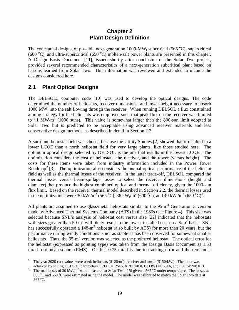
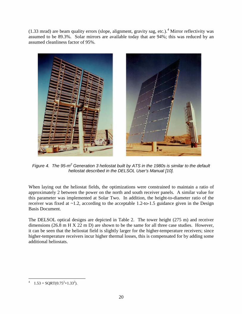
(1.33 mrad) are beam quality errors (slope, alignment, gravity sag, etc.).4 Mirror reflectivity was assumed to be 89.3%. Solar mirrors are available today that are 94%; this was reduced by an assumed cleanliness factor of 95%.

Figure 4. The 95-m2 Generation 3 heliostat built by ATS in the 1980s is similar to the default heliostat described in the DELSOL User’s Manual [10].

When laying out the heliostat fields, the optimizations were constrained to maintain a ratio of approximately 2 between the power on the north and south receiver panels. A similar value for this parameter was implemented at Solar Two. In addition, the height-to-diameter ratio of the receiver was fixed at ~1.2, according to the acceptable 1.2-to-1.5 guidance given in the Design Basis Document. The DELSOL optical designs are depicted in Table 2. The tower height (275 m) and receiver dimensions (26.8 m H X 22 m D) are shown to be the same for all three case studies. However, it can be seen that the heliostat field is slightly larger for the higher-temperature receivers; since higher-temperature receivers incur higher thermal losses, this is compensated for by adding some additional heliostats.

4 1.53 = SQRT(0.752+1.332).

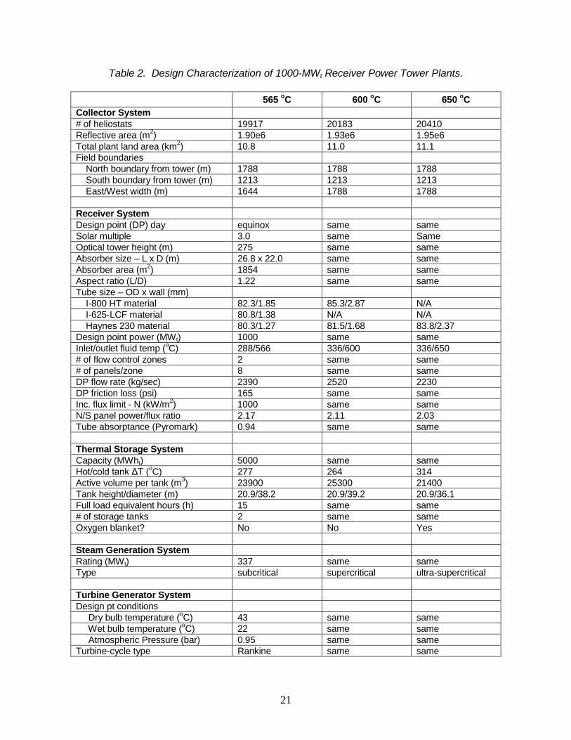
21

Table 2. Design Characterization of 1000-MWt Receiver Power Tower Plants.

565 oC 600 oC 650 oC Collector System # of heliostats 19917 20183 20410 Reflective area (m2) 1.90e6 1.93e6 1.95e6 Total plant land area (km2) 10.8 11.0 11.1 Field boundaries North boundary from tower (m) 1788 1788 1788 South boundary from tower (m) 1213 1213 1213 East/West width (m) 1644 1788 1788 Receiver System Design point (DP) day equinox same same Solar multiple 3.0 same Same Optical tower height (m) 275 same same Absorber size – L x D (m) 26.8 x 22.0 same same Absorber area (m2) 1854 same same Aspect ratio (L/D) 1.22 same same Tube size – OD x wall (mm) I-800 HT material 82.3/1.85 85.3/2.87 N/A I-625-LCF material 80.8/1.38 N/A N/A Haynes 230 material 80.3/1.27 81.5/1.68 83.8/2.37 Design point power (MWt) 1000 same same Inlet/outlet fluid temp (oC) 288/566 336/600 336/650 # of flow control zones 2 same same # of panels/zone 8 same same DP flow rate (kg/sec) 2390 2520 2230 DP friction loss (psi) 165 same same Inc. flux limit - N (kW/m2) 1000 same same N/S panel power/flux ratio 2.17 2.11 2.03 Tube absorptance (Pyromark) 0.94 same same Thermal Storage System Capacity (MWht) 5000 same same Hot/cold tank ΔT (oC) 277 264 314 Active volume per tank (m3) 23900 25300 21400 Tank height/diameter (m) 20.9/38.2 20.9/39.2 20.9/36.1 Full load equivalent hours (h) 15 same same # of storage tanks 2 same same Oxygen blanket? No No Yes Steam Generation System Rating (MWt) 337 same same Type subcritical supercritical ultra-supercritical Turbine Generator System Design pt conditions Dry bulb temperature (oC) 43 same same Wet bulb temperature (oC) 22 same same Atmospheric Pressure (bar) 0.95 same same Turbine-cycle type Rankine same same

22

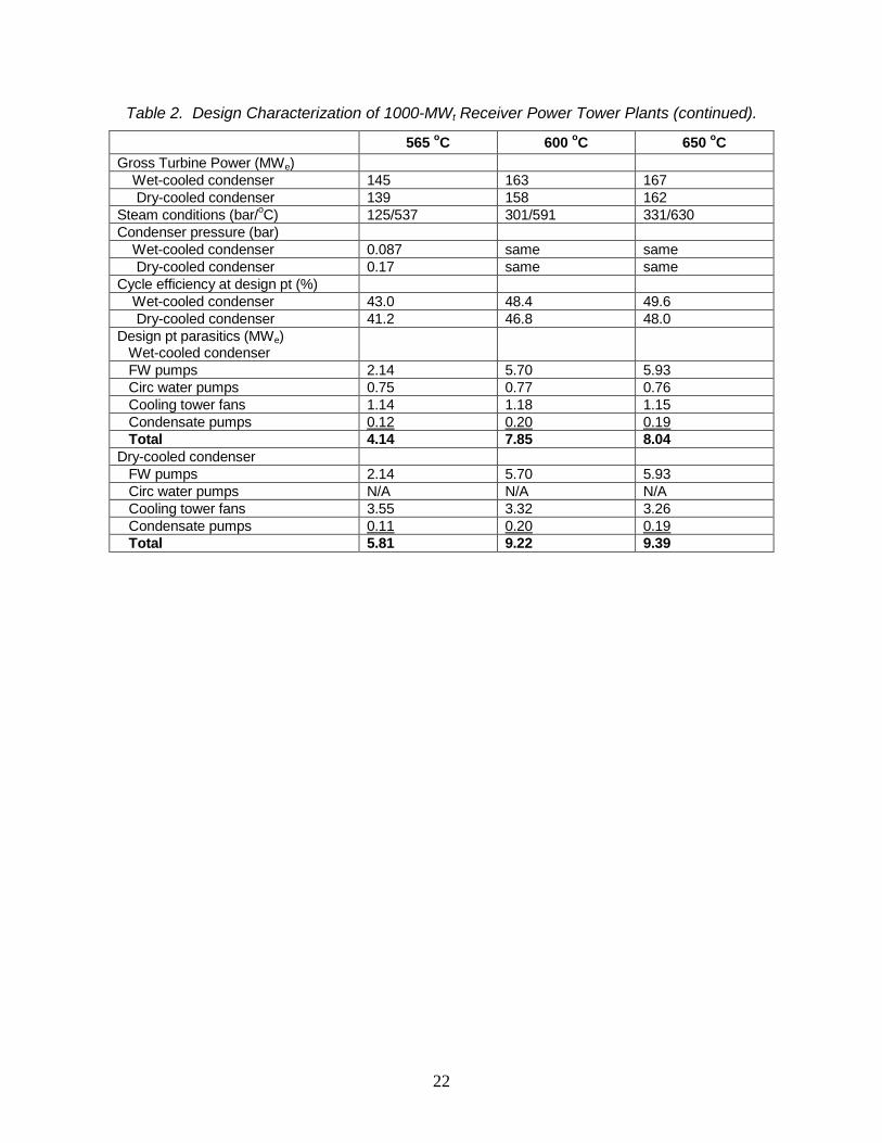
Table 2. Design Characterization of 1000-MWt Receiver Power Tower Plants (continued).

565 oC 600 oC 650 oC Gross Turbine Power (MWe) Wet-cooled condenser 145 163 167 Dry-cooled condenser 139 158 162 Steam conditions (bar/oC) 125/537 301/591 331/630 Condenser pressure (bar) Wet-cooled condenser 0.087 same same Dry-cooled condenser 0.17 same same Cycle efficiency at design pt (%) Wet-cooled condenser 43.0 48.4 49.6 Dry-cooled condenser 41.2 46.8 48.0 Design pt parasitics (MWe) Wet-cooled condenser

FW pumps 2.14 5.70 5.93 Circ water pumps 0.75 0.77 0.76 Cooling tower fans 1.14 1.18 1.15 Condensate pumps 0.12 0.20 0.19 Total 4.14 7.85 8.04 Dry-cooled condenser FW pumps 2.14 5.70 5.93 Circ water pumps N/A N/A N/A Cooling tower fans 3.55 3.32 3.26 Condensate pumps 0.11 0.20 0.19 Total 5.81 9.22 9.39

23

2.2 Receiver Designs The receiver system design is assumed to be similar to that demonstrated at Solar Two. A system schematic is shown in Figure 5. Molten salt is pumped up the tower, fills a cold-surge tank that is pressurized with air,5 and then flows through the receiver. Receiver absorber materials of historical and current interest were studied: Incoloy 800H (I-800H), Inconel 625-LCF, and Haynes 230. Incoloy was selected because it was the tube material used in a salt receiver test at SNL [23] before Solar Two6 and was also used in the Solar One steam receiver. Inconel 625-LCF was selected because it was extensively studied by industry and SNL after Solar Two as a possible next-generation material [25]. Haynes 230 was selected because it has been recently promoted as an excellent candidate material for solar dish and tower receivers by the material manufacturer.7 These materials were also selected because they are identified as candidate high-temperature tube materials within the ASME Boiler and Pressure Vessel Code. The chemical compositions of these three materials are shown in Table 3.

Figure 5. Receiver system schematic.

5 The primary function of the cold surge tank (also known as inlet tank) is to provide emergency receiver cooling

for a few minutes during station blackout. Given loss of AC power, the cold salt pumps will trip and the emergency power system will be used to quickly remove the heliostat beams from the receiver.

6 The tube material used at Solar Two was 316H SS. This material is not recommended in future salt receivers because it was found to be susceptible to stress-corrosion cracking [24].

7 According to data and analysis presented by Dr. Henry White (Haynes International) to SNL in August 2010, Haynes 230 is more thermally stable than I800 and Inconel 625-LCF alloys. Thus, the creation of deleterious phases that lead to embrittlement are less of a concern when operating above 600 oC.

24

Table 3. Receiver Tube Material Composition. [26], [27], [28]

Incoloy 800 HT Inconel 625-LCF Haynes 230 Nickel 30-35% 58% 57%

Chromium 19-23% 20-23% 22% Tungsten 14%

Molybdenum 8-10% 2% Iron 39.5% 5% 3%

Cobalt 1% 5% Manganese 0.5% 0.5%

Silicon 0.15% 0.4% Aluminum 0.25-0.6% 0.40% 0.3%

Carbon 0.06-0.1% 0.03% 0.1% Lanthanum 0.02%

Boron 0.015% Titanium 0.25-0.6% 0.4% Niobium 3.15-4.15% Sulfur 0.015%

Phosphorus 0.015% Nitrogen 0.02%

When the metal that comprises the tubes of the receiver is heated, it expands.8 Some of this expansion is accommodated in the receiver design by allowing the panels to grow in length. Some of this expansion, however, cannot be accommodated and so produces mechanical strains as heated metal constrained by colder material. These strains are termed “thermal strains” and result from “self constraint.” A solar receiver must, by its nature, operate cyclically. The receiver is heated to operating temperature and then allowed to relax to thermal equilibrium at least daily, and more often due to the passage of clouds over the plant. This cyclic operation results in thermal fatigue damage to the receiver tubes. This fatigue damage must be limited to a tolerable level over the 30-year lifetime of the receiver. Fatigue damage data were compiled from several sources; low-cycle fatigue (LCF) experimental data were adapted and used. The LCF data for the alloys investigated in this study appear in Table 4. It can be seen that the number of cycles to failure decreases as strain and/or temperature increases. Of the three alloys, I-800 has (by far) the most available data since it is the oldest alloy. The LCF data apply to relatively short strain cycles; a few-second strain cycle was typical. Strain cycles within a power tower typically last several hours, which calls into question the applicability of the few-second LCF data available in the literature. Previous experimental studies have shown that cyclic fatigue life is significantly reduced given long hold periods of an hour or more [31] [32] [33]. To obtain an answer to this question, longer cycle LCF data were 8 This section follows much of the general methodology described in Reference 29, and some of the text from that

paper has been reused here.

25

sought. Five-hour hold data were found for I-800 [33], but only four data points were identified. In Figure 6 these four points are plotted on top of the short-cycle LCF data published on the Special Metals website for I-800 type alloys [26]. The average of these plots suggests that fatigue life can be expected to be reduced by an approximate factor of 4 due to long hold times. This factor is also suggested by data in a paper comparing 10-second and 60-minute hold times for I-800 [32], and comparing 0- and 30-minute hold times for Inconel 625 [34]. Thus, in this study the cycles-to-failure shown in Table 4 were multiplied by a factor of ¼. These reduced values represent the allowable number of cycles for a given strain range and temperature. Table 4. Number of Fatigue Cycles to Failure for I-800H [26], Inconel 625-LCF [27 and 29], and

Haynes 230 [30] as a Function of Strain at Temperature. (These values were multiplied by ¼ in the analysis.)

StrainI800H 0.001 0.002 0.003 0.004 0.005 0.006 0.007 0.008

70 1.00E+07 1.00E+06 1.00E+05 7.00E+04 5.00E+04 2.50E+04 1.70E+04 1.30E+04Temp F 1000 1.00E+07 1.00E+06 1.00E+05 7.00E+04 2.60E+04 1.40E+04 1.00E+04 8.00E+03

1200 1.00E+06 1.00E+05 5.00E+04 2.50E+04 1.30E+04 8.00E+03 6.00E+03 4.00E+031400 7.00E+05 9.00E+04 2.30E+04 1.00E+04 7.00E+03 4.00E+03 3.20E+03 2.50E+03

StrainInconel 625 LCF 0.002 0.004 0.006 0.008 0.01 0.02

1000 1.00E+09 1.00E+07 1.00E+06 9.33E+04 3.63E+04 1.12E+03Temp F 1200 1.00E+08 3.63E+05 1.66E+04 3.72E+03 1.38E+03 1.62E+02

1500 1.00E+07 3.63E+04 3.72E+03 1.38E+03 5.89E+02 1.00E+02 Strain

Haynes 230 0.003 0.004 0.005 0.0055 0.0065 0.007 0.008 0.01 0.015 0.02800 1.00E+06 4.47E+05 1.86E+05 1.20E+05 3.98E+04 2.88E+04 1.48E+04 7.59E+03 2.24E+03 1.00E+03

Temp F 1400 2.00E+05 7.59E+04 8.13E+03 6.46E+03 5.13E+03 3.16E+03 2.04E+03 8.51E+02 5.01E+02 1.58E+02 Kistler [35] pointed out that the strain cycles experienced by a solar receiver vary in magnitude. This is because the receiver power level varies each day, and each cloud passage is different. Considerable advantage can be gained by accounting for the smaller cycles using a “linear damage rule” relative to treating all cycles as full cycles. This can be accomplished by first establishing the number of cycles expected and their range over the receiver lifetime. This accounting has been performed based upon data taken at the Solar One pilot plant, by tabulating cycles in the direct-normal insolation measured at the ground. The accounting is complex because each cycle has both a high and a low value of insolation. The cycles reported in Kistler can, however, be grouped by their range, assuming that cycles of the same range are equally damaging, regardless of their mean. The number of cycles in ten range groupings is shown in Figure 7. The cumulative damage resulting from these cycles can be calculated from the linear damage rule:

f

n

i ia

i DNN

=∑=1 ,

(1)

26

Figure 6. Low-cycle fatigue strength for I-800, I-800H, and I-800HT alloys at temperatures from 70 oF to 1400 oF [26]. Curves appear to have short hold times.9 Black squares are data from

four tests of I800 reported in Reference 33 given 5-hour hold times.

Figure 7. Number of strain cycles. 9 According to an email sent from Lew Shoemaker (Special Metals) to G. Kolb (SNL) on December 2, 2009, the I-

800 data is old and fatigue-cycle time is unknown. However, comparing the curve for I800 at 1200 oF with a similar curve found in Reference 32 suggests that the cycle time was ~10 seconds or less.

27

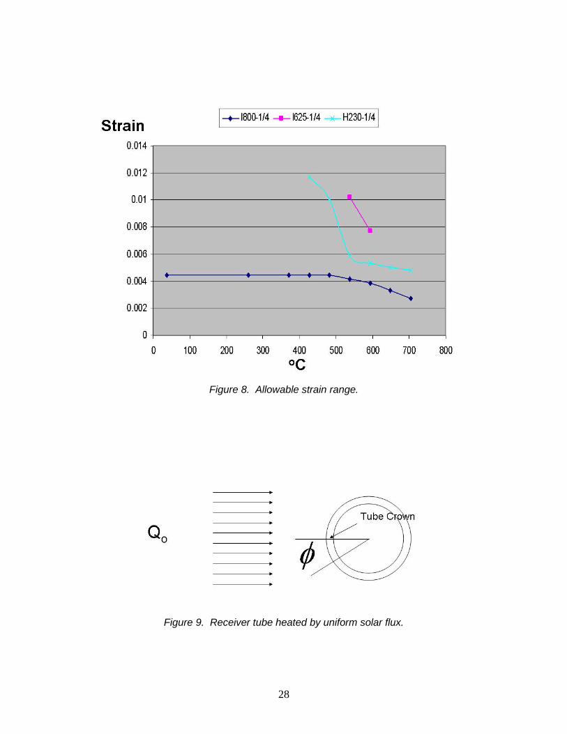
The allowable strain e. is defined as the full-range strain that results in a cumulative damage of 1 (failure) for the combination of cycles. An example of this calculation is presented in Table 5 for I-800H at a temperature of 1100 °F. In this example, the allowable strain range is found to be 0.00386. This strain corresponds to an allowable number of cycles of 12,800. For this case, the 98,900 cycles in the histogram are found to be equivalent to 12,800 full-range cycles. Similar calculations were performed for the range of tube temperatures anticipated in the operation of the receiver. An EXCEL spreadsheet was developed to perform the iterative calculations needed to determine the strain range that results in a cumulative damage of unity, for each temperature. The spreadsheet was also used to perform a linear interpolation of the cycles-to-failure values shown in Table 4. The resulting allowable strain-range curves for the three alloys are shown in Figure 8.

Table 5. Linear Damage Calculation for Incoloy 800H at 1100 oF (593 oC).

Design Strain 3.86e-03 Allowable Cycles 12800

Cycle Range Strain Range Number of Cycles

Allowable Cycles Lifetime

10% 3.86e-04 41100 20% 7.72e-04 15300 30% 1.16e-03 8900 1.18e+06 0.008 40% 1.54e-03 6900 7.02e+05 0.010 50% 1.93e-03 4900 2.24e+05 0.022 60% 2.32e-03 4000 1.00e+04 0.040 70% 2.70e-03 4200 5.41e+04 0.078 80% 3.09e-03 4800 1.81e+04 0.265 90% 3.47e-03 8000 1.55e+04 0.516 100% 3.86e-03 800 1.28e+04 0.062

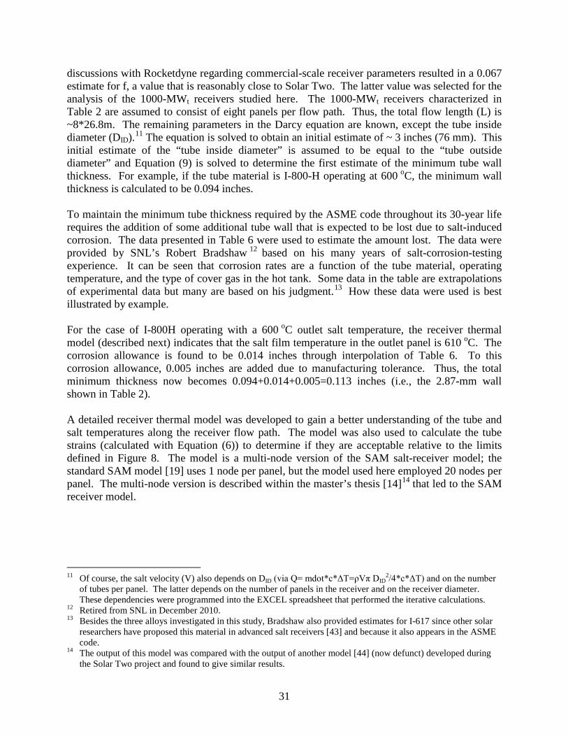
Total Cycles: 98900 Cumulative Damage: 1 Given the allowable strain range, the next step in the absorber tube design process was to derive the allowable heat flux. The allowable heat flux is defined as that heat flux that results in the allowable strain range. Consider a receiver tube heated by solar radiation as shown in Figure 9. The heat flux can be assumed to be nearly entirely spectral. Given this, the heat flux normal to the surface of the tube will have a cosine distribution owing to the curvature of the tube. )cos(φon qq = (2)

28

Figure 8. Allowable strain range.

Figure 9. Receiver tube heated by uniform solar flux.

29

Because the tube wall is thin relative to the tube diameter, it can be assumed that the heat flux conducts one-dimensionally through a thin tube wall into the molten salt. The wall temperature will be governed in this case by the following formulas:

( )

tTT

kq ion

−= (3)

( )sin TThq −= (4) The convection heat transfer coefficient that is determined from the Gnielinski correlation for turbulent flow in tubes is:

( )( )

( ) ( )1Pr8/7.121Pr1000Re8/

3221 −+−

=f

fNu DD (5)

The highest metal temperature will occur on the tube crown at the outside surface of the tube. This location will develop the highest compressive thermal stress due to the heating. Assuming that the tube remains straight (a plane-strain assumption) the mechanical strain that results is approximately the sum of the strain due to the through-thickness temperature difference, and the front-to-back temperature difference. The resulting formula for strain is Reference 36 :

[ ]( )

−

++

−−

= aveicocicoc T

TTTT212 ν

αε (6)

where ε is the strain, α is the coefficient of thermal expansion, ν is Poisson’s ratio, Toc is the outer crown temperature, Tic is the inner crown temperature, and Tavg is the average circumferential temperature. The average temperature of the cross section can be found from the expression:

π

πφπ

π

22

2

2∫− +

+

=s

io

ave

TdTT

T (7)

If Equations (2), (3), and (4), are substituted into Equation (7) to solve for Tave , one gets:

( )

π

sicoc

save

TTT

TT−

+

+=2 (8)

Equation (6) can be employed to derive an equation for the allowable heat flux for a given tube diameter and tube-wall thickness. For every salt temperature, there exists a heat flux that results in a strain and temperature at the tube crown that intersects the allowable strain curve of Figure

30

8. Because the material properties depend on temperature, an iterative process is required to establish this flux limit. The discussion thus far has focused on design of the receiver tubes to achieve a 30-year fatigue life. In addition to fatigue, the tube design should meet or exceed the requirements of the ASME Boiler and Pressure Vessel code [37], as well as be tolerant to the expected amount of salt-induced corrosion. Section I of the ASME Code stipulates the method to determine minimum tube-wall thickness.10 The thickness is a function of the operating pressure, temperature, and type of tube material. The relevant equations described in the code are

DPS

PDt 005.02

++

= (9)

−−−

=)005.0(

01.02DtD

DtSP (10)

where P = maximum fluid pressure (psi), D = tube outside diameter (inches), S = maximum allowable stress of tube material obtained from ASME Section II tables in PG-23 that show allowable stress versus operating temperature (psi) for each of the three alloys, and t = minimum required tube-wall thickness (inches). The maximum salt-fluid pressure (P) was selected to be 230 psi. The delta P across the Solar Two receiver was ~165 psi (60.4 m of head) and is also the approximate design delta P for commercial-scale receivers. The value of 230 was selected to add a 30% safety margin that might occur during abnormal events. (Pressures in this range are also similar to the operating pressure of the inlet salt tank located at the receiver inlet.) The value for outside diameter (D) was calculated via an iterative procedure programmed within an EXCEL worksheet. The Darcy-Weisbach equation

g

VDLfhID

f 2

2

= (11)

was first used to estimate an overall friction factor (f) for the Solar Two receiver. Data acquisition records collected during operation on September 13, 1998, were examined. Solution of the Darcy equation to match the test data produced a 0.054 estimate for f. In addition,

10 Section I of the code (Rules for Construction of Power Boilers) is primarily intended for water boilers. However,

as explained in the introduction to Section I, “…. the rules of this Section are not intended to apply to thermal fluid heaters in which a fluid other than water is heated by the application of heat resulting from the combustion of solid, liquid, or gaseous fuel but in which no vaporization of the fluid takes place; however, such thermal fluid heaters may be constructed and stamped in accordance with this Section, provided all applicable requirements are met ….” The molten-salt receivers designed in this report are “thermal fluid heaters” that meet the Section I criteria.

31

discussions with Rocketdyne regarding commercial-scale receiver parameters resulted in a 0.067 estimate for f, a value that is reasonably close to Solar Two. The latter value was selected for the analysis of the 1000-MWt receivers studied here. The 1000-MWt receivers characterized in Table 2 are assumed to consist of eight panels per flow path. Thus, the total flow length (L) is ~8*26.8m. The remaining parameters in the Darcy equation are known, except the tube inside diameter (DID).11 The equation is solved to obtain an initial estimate of ~ 3 inches (76 mm). This initial estimate of the “tube inside diameter” is assumed to be equal to the “tube outside diameter” and Equation (9) is solved to determine the first estimate of the minimum tube wall thickness. For example, if the tube material is I-800-H operating at 600 oC, the minimum wall thickness is calculated to be 0.094 inches. To maintain the minimum tube thickness required by the ASME code throughout its 30-year life requires the addition of some additional tube wall that is expected to be lost due to salt-induced corrosion. The data presented in Table 6 were used to estimate the amount lost. The data were provided by SNL’s Robert Bradshaw 12 based on his many years of salt-corrosion-testing experience. It can be seen that corrosion rates are a function of the tube material, operating temperature, and the type of cover gas in the hot tank. Some data in the table are extrapolations of experimental data but many are based on his judgment.13 How these data were used is best illustrated by example. For the case of I-800H operating with a 600 oC outlet salt temperature, the receiver thermal model (described next) indicates that the salt film temperature in the outlet panel is 610 oC. The corrosion allowance is found to be 0.014 inches through interpolation of Table 6. To this corrosion allowance, 0.005 inches are added due to manufacturing tolerance. Thus, the total minimum thickness now becomes 0.094+0.014+0.005=0.113 inches (i.e., the 2.87-mm wall shown in Table 2). A detailed receiver thermal model was developed to gain a better understanding of the tube and salt temperatures along the receiver flow path. The model was also used to calculate the tube strains (calculated with Equation (6)) to determine if they are acceptable relative to the limits defined in Figure 8. The model is a multi-node version of the SAM salt-receiver model; the standard SAM model [19] uses 1 node per panel, but the model used here employed 20 nodes per panel. The multi-node version is described within the master’s thesis [14]14 that led to the SAM receiver model.

11 Of course, the salt velocity (V) also depends on DID (via Q= mdot*c*ΔT=ρVπ DID

2/4*c*ΔT) and on the number of tubes per panel. The latter depends on the number of panels in the receiver and on the receiver diameter. These dependencies were programmed into the EXCEL spreadsheet that performed the iterative calculations.

12 Retired from SNL in December 2010. 13 Besides the three alloys investigated in this study, Bradshaw also provided estimates for I-617 since other solar

researchers have proposed this material in advanced salt receivers [43] and because it also appears in the ASME code.

14 The output of this model was compared with the output of another model [44] (now defunct) developed during the Solar Two project and found to give similar results.

32

Table 6. Salt Corrosion Estimates as a Function of Salt Temperature and Cover Gas.

Mils of Total Corrosion after 10 yrs - With Air Blanket -

Mils of Total Corrosion after 10 yrs - With Oxygen Blanket -

600 oC 625 oC 650 oC 600 oC 625 oC 650 oC

I-625-LCF 3*

a P 10 20 a P 3 6 10

b P

I-800H 3 d S

30 e f L

60 e L 10 c L 2 20 40

I-617 2 6 10 c L 2 4 7

Haynes 230 Slightly worse than I-625-LCF

Extrapolations based on data are underlined. Other values are estimates. 1 Mil = 0.001 inch Key: P power law kinetics, time0.7 L linear kinetics S square-root (parabolic) kinetics, time0.5 * thermal-cycling test, all others isothermal a SAND2000-8240 [38] b SAND2001-8758 [25] c APC, J. Metals, 1985 [39] d SAND82-8911, 600 oC loops report [40] e SAND86-9009, 605-630 oC hot corrosion report [41] f SAND82-8210, 630 oC loops report [42] Assumptions:

1. 10 years of continuous corrosion is equivalent to 30 years of receiver operation because the receiver is assumed to be filled with salt 8 hours per day.

2. Isothermal data extrapolations are valid for thermally cycled receiver conditions. 3. Difference between air or oxygen blanket is negligible at 600 oC but significant at 650 oC. 4. I-617 corrodes no faster than I-625 because compositions of alloys are similar. I-617 is expected

to corrode somewhat slower based on aluminum addition. Data in APC report for other test conditions support this assumption.

5. Molten-salt composition (oxide ion content) depends on Tmax in hot-salt storage tank. Kinetics are too slow for chemical shift corresponding to tube film temperature during a single receiver pass.

6. Data for Alloy 800-standard grade apply to I-800H. 7. Compression of oxide scale on ID of tubes may be beneficial for scale adherence after

substantial thickening. 8. For Haynes 230, Bradshaw’s statement of “slightly worse” was assumed to be 20% worse.

33

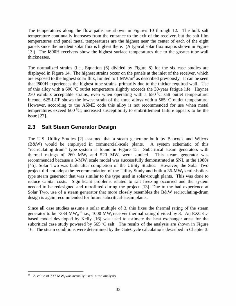
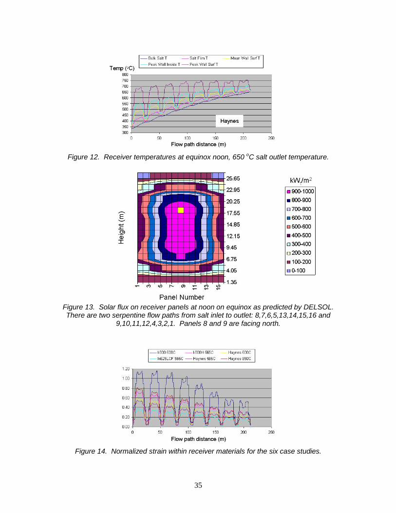
The temperatures along the flow paths are shown in Figures 10 through 12. The bulk salt temperature continually increases from the entrance to the exit of the receiver, but the salt film temperatures and panel metal temperatures are the highest near the center of each of the eight panels since the incident solar flux is highest there. (A typical solar flux map is shown in Figure 13.) The I800H receivers show the highest surface temperatures due to the greater tube-wall thicknesses. The normalized strains (i.e., Equation (6) divided by Figure 8) for the six case studies are displayed in Figure 14. The highest strains occur on the panels at the inlet of the receiver, which are exposed to the highest solar flux, limited to 1 MW/m2 as described previously. It can be seen that I800H experiences the highest tube strains, primarily due to the thicker required wall. Use of this alloy with a 600 oC outlet temperature slightly exceeds the 30-year fatigue life. Haynes 230 exhibits acceptable strains, even when operating with a 650 oC salt outlet temperature. Inconel 625-LCF shows the lowest strain of the three alloys with a 565 oC outlet temperature. However, according to the ASME code this alloy is not recommended for use when metal temperatures exceed 600 oC; increased susceptibility to embrittlement failure appears to be the issue [27]. 2.3 Salt Steam Generator Design The U.S. Utility Studies [2] assumed that a steam generator built by Babcock and Wilcox (B&W) would be employed in commercial-scale plants. A system schematic of this “recirculating-drum” type system is found in Figure 15. Subcritical steam generators with thermal ratings of 260 MWt and 520 MWt were studied. This steam generator was recommended because a 3-MWt scale model was successfully demonstrated at SNL in the 1980s [45]. Solar Two was built after completion of the Utility Studies. However, the Solar Two project did not adopt the recommendation of the Utility Study and built a 36-MWt kettle-boiler-type steam generator that was similar to the type used in solar-trough plants. This was done to reduce capital costs. Significant problems related to salt freezing occurred and the system needed to be redesigned and retrofitted during the project [13]. Due to the bad experience at Solar Two, use of a steam generator that more closely resembles the B&W recirculating-drum design is again recommended for future subcritical-steam plants. Since all case studies assume a solar multiple of 3, this fixes the thermal rating of the steam generator to be ~334 MWt,15 i.e., 1000 MWt receiver thermal rating divided by 3. An EXCEL-based model developed by Kelly [16] was used to estimate the heat exchanger areas for the subcritical case study powered by 565 oC salt. The results of the analysis are shown in Figure 16. The steam conditions were determined by the GateCycle calculations described in Chapter 3.

15 A value of 337 MWt was actually used in the analysis.

34

Figure 10. Receiver temperatures at equinox noon, 565 oC salt outlet temperature.


35


Figure 13. Solar flux on receiver panels at noon on equinox as predicted by DELSOL. There are two serpentine flow paths from salt inlet to outlet: 8,7,6,5,13,14,15,16 and

9,10,11,12,4,3,2,1. Panels 8 and 9 are facing north.

Figure 14. Normalized strain within receiver materials for the six case studies.

36

Figure 15. Steam generator system schematic proposed by Babcock and Wilcox [2].

No detailed designs currently exist for molten-salt steam generators that operate at supercritical and ultra-supercritical steam conditions. Kelly explored a concept [16], but much further work is required. Using Kelly’s first-order model, heat exchanger areas were estimated for a supercritical steam generator powered by 600 oC salt. The results of the analysis are given in Figure 17. The system configuration is simpler than a subcritical steam generator because there is no steam boiling regime.

37

Figure 16. Subcritical molten-salt steam generator heat balance.

38

Figure 17. Supercritical molten-salt steam generator heat balance.

2.4 Balance of Plant A two-tank thermal storage system, similar to that demonstrated at Solar Two, is assumed. The tank sizes given in Table 2 were determined using the SAM algorithm [19] given the assumed hot tank and cold tank temperatures for each case study. The tank dimensions necessary to achieve 15 hours of storage are nominally 21 m tall and 38.5 m in diameter. This is somewhat larger than the salt tanks currently operating at the Andasol trough plants.16 The cold tank temperature for the 565 oC case is the same as at Solar Two, i.e., 288 oC. The cold tank temperature selected for the 600 and 650 oC cases are somewhat higher than Solar Two (336 oC) because the GateCycle analysis of the power cycle suggested that a higher-power conversion system efficiency can be achieved with this return temperature. As described next, supercritical plants have a higher feedwater temperature. This will result in a higher salt return temperature to the cold tank (compare the feedwater and salt return temperatures in Figure 16 and 17).

16 The Andasol solar trough plants are using the largest molten-salt tanks currently in existence. They are 14 m tall

by 38.5 m in diameter. The cold tank temperature is the same as analyzed here, but the hot tank is only 390 oC.

39

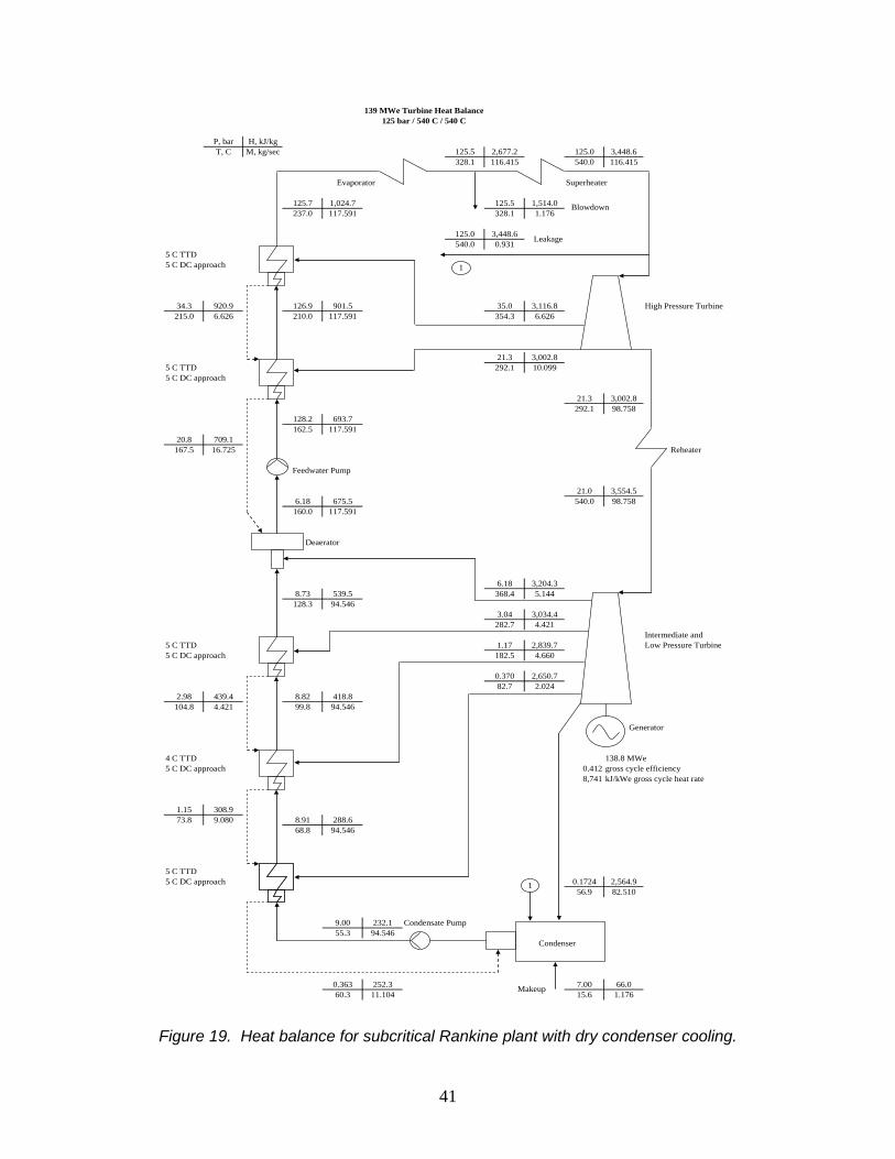
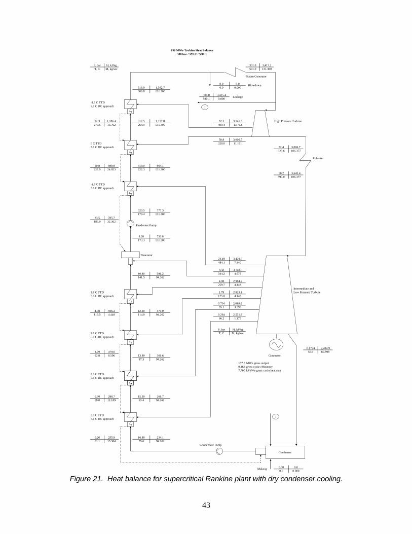
The steam turbine system designs are assumed to be similar to subcritical and supercritical designs found in today’s coal-fired power plants. As shown in Table 2, gross turbine system output is different for each case study given an identical 337 MWt thermal input from the steam generator. The different electrical outputs (from 139 to 167 MWe) are caused by variations in thermal-to-electric conversion efficiency. With supercritical pressures, because of the greater steam pressure range in the turbine from inlet through to the condenser, there is greater scope for including an extra stage or stages of feedwater heating; for example, the subcritical cycles depicted in Figures 18 and 19 incorporate 5 closed and 1 open heater and the supercritical cycles shown in Figures 20 through 23 have 7 closed and 1 open heater. This enables an even higher feedwater temperature to be achieved in supercritical cycles and thereby provide a further increase in cycle efficiency. Typical feedwater temperatures are ~300 °C compared to ~240 °C for sub-critical plants. Subcritical coal-fired plants currently exist in the 150-MWe power range. However, the smallest supercritical plants are greater than 400 MWe

17. Thus, it is assumed that supercritical technology can be successfully scaled down to the 150-MWe power range. It is also assumed that it is not practical to thermally cycle a supercritical-power block on a daily basis; it will need to operate nearly 24/7, much like it does in a coal plant. The much higher steam pressures (≥300 bar supercritical versus 125 bar subcritical) will result in very thick pipe walls and turbine casings, which should greatly increase startup time relative to a subcritical plant. Future solar power plants will likely require the use of dry-cooled condensers to reduce water consumption. Dry-cooling technology similar to that offered by SPX Cooling Technologies is assumed in the analysis. According to SPX design specifications [8], the air-side delta P across the cooling coils can be estimated to be ~1.5 mbar and the fan power required by each bay is ~200 hp. These parameters, along with the amount of rejected heat calculated by GateCycle, were used to determine the number of cooling bays. The design condition was the hottest time of the year (42.8 oC), a condenser design pressure of 0.17 bar (versus a typical value of 0.087 bar for wet-cooled plants), and a design initial-temperature difference (ITD) of 14 oC. 18 these assumptions were found to optimize the annual performance of dry-cooled solar trough plants [9].

17 Ansaldo is offering a 200 MW supercritical steam turbine but detailed information about it could not be found.

See www.ansaldoenergia.com. 18 ITD is defined as condenser temperature minus ambient temperature.

40

145 MWe Turbine Heat Balance125 bar / 540 C / 540 C

P, bar H, kJ/kgT, C M, kg/sec 125.5 2,677.2 125.0 3,448.6

328.1 116.415 540.0 116.415

Evaporator Superheater

125.7 1,024.7 125.5 1,514.0237.0 117.591 328.1 1.176

125.0 3,448.6540.0 0.931

5 C TTD5 C DC approach

34.3 920.9 126.9 901.5 35.0 3,116.8 High Pressure Turbine215.0 6.626 210.0 117.591 354.3 6.626

21.3 3,002.85 C TTD 292.1 10.0995 C DC approach

21.3 3,002.8292.1 98.758

128.2 693.7162.5 117.591

20.8 709.1167.5 16.725 Reheater

Feedwater Pump

21.0 3,554.56.18 675.5 540.0 98.758160.0 117.591

Deaerator

6.18 3,209.78.73 539.5 371.0 4.925128.3 95.941

3.04 3,040.4285.7 4.476

Intermediate and5 C TTD 1.17 2,846.1 Low Pressure Turbine5 C DC approach 185.7 4.717

0.370 2,655.985.4 3.784

2.98 439.4 8.82 418.8104.8 4.476 99.8 95.941

Generator

4 C TTD 145.1 MWe5 C DC approach 0.430 gross cycle efficiency

8,365 kJ/kWe gross cycle heat rate

1.15 308.973.8 9.193 8.91 288.6

68.8 95.941

5 C TTD5 C DC approach 0.0874 2,484.2

43.2 80.857

9.00 182.1 Condensate Pump43.3 95.941

Condenser

0.363 202.3 1.03 65.448.3 12.977 15.6 1.176

1

1

Blowdown

Leakage

Makeup

Figure 18. Heat balance for subcritical Rankine plant with wet condenser cooling.

41


P, bar H, kJ/kgT, C M, kg/sec 125.5 2,677.2 125.0 3,448.6

328.1 116.415 540.0 116.415

Evaporator Superheater

125.7 1,024.7 125.5 1,514.0237.0 117.591 328.1 1.176

125.0 3,448.6540.0 0.931

5 C TTD5 C DC approach

34.3 920.9 126.9 901.5 35.0 3,116.8 High Pressure Turbine215.0 6.626 210.0 117.591 354.3 6.626

21.3 3,002.85 C TTD 292.1 10.0995 C DC approach

21.3 3,002.8292.1 98.758

128.2 693.7162.5 117.591

20.8 709.1167.5 16.725 Reheater

Feedwater Pump

21.0 3,554.56.18 675.5 540.0 98.758160.0 117.591

Deaerator

6.18 3,204.38.73 539.5 368.4 5.144128.3 94.546

3.04 3,034.4282.7 4.421

Intermediate and5 C TTD 1.17 2,839.7 Low Pressure Turbine5 C DC approach 182.5 4.660

0.370 2,650.782.7 2.024

2.98 439.4 8.82 418.8104.8 4.421 99.8 94.546

Generator

4 C TTD 138.8 MWe5 C DC approach 0.412 gross cycle efficiency

8,741 kJ/kWe gross cycle heat rate

1.15 308.973.8 9.080 8.91 288.6

68.8 94.546

5 C TTD5 C DC approach 0.1724 2,564.9

56.9 82.510

9.00 232.1 Condensate Pump55.3 94.546

Condenser

0.363 252.3 7.00 66.060.3 11.104 15.6 1.176

1

1

Blowdown

Leakage

Makeup

Figure 19. Heat balance for subcritical Rankine plant with dry condenser cooling.

42


P, bar H, kJ/kg 301.0 3,417.2T, C M, kg/sec 591.0 131.200

Steam Generator

0.0 0.0316.0 1,362.7 0.0 0.000306.8 131.200

300.0 3,415.4590.1 0.197

-1.7 C TTD5.6 C DC approach

92.3 1,186.4 317.5 1,157.8 92.3 3,141.5 High Pressure Turbine270.5 13.751 264.9 131.200 409.4 13.751

50.8 3,006.70 C TTD 328.0 11.1525.6 C DC approach 52.4 3,006.7

329.6 106.100

Reheater

50.8 980.8 319.0 964.1227.9 24.903 222.3 131.200

50.2 3,643.4590.0 106.100


320.5 777.3179.4 131.200

23.5 785.7185.0 32.337

Feedwater Pump

8.58 733.8173.3 131.200

Deaerator23.49 3,429.0484.1 7.434

8.58 3,148.810.80 596.2 344.2 4.672141.5 94.185

4.08 2,986.6260.9 4.440

Intermediate and2.8 C TTD 1.79 2,827.3 Low Pressure Turbine5.6 C DC approach 177.9 4.138

0.704 2,674.197.2 3.584

4.08 596.2 12.30 479.0119.5 4.440 114.0 94.190 0.264 2,537.3

66.2 2.941

P, bar H, kJ/kg2.8 C TTD T, C M, kg/sec5.6 C DC approach

0.0874 2,409.11.79 479.0 43.2 78.89292.8 8.578 13.80 366.6 Generator

87.3 94.192163.1 MWe gross output0.484 gross cycle efficiency7,441 kJ/kWe gross cycle heat rate

2.8 C TTD5.6 C DC approach

0.70 288.7 15.30 266.769.0 12.162 63.4 94.192


0.26 204.8 16.80 183.048.9 15.103 43.4 94.192

Condensate Pump

Condenser

0.00 0.00.0 0.000

1

1

Blowdown

Leakage

Makeup

Figure 20. Heat balance for supercritical Rankine plant with wet condenser cooling.

43



Steam Generator

0.0 0.0316.0 1,362.7 0.0 0.000306.8 131.300

300.0 3,415.4590.1 0.000




329.6 106.377

Reheater

50.8 980.8 319.0 964.1227.9 24.923 222.3 131.300

50.2 3,643.4590.0 106.377


320.5 777.3179.4 131.300

23.5 785.7185.0 32.362

Feedwater Pump

8.58 733.8173.3 131.300

Deaerator23.49 3,429.0484.1 7.440

8.58 3,148.810.80 596.2 344.2 4.676141.5 94.262

4.08 2,984.2259.7 4.448


0.704 2,669.895.1 3.593

4.08 596.2 12.30 479.0119.5 4.448 114.0 94.262 0.264 2,531.8

66.2 1.175


0.1724 2,484.91.79 479.0 56.9 80.89892.8 8.596 13.80 366.6 Generator



0.70 288.7 15.30 266.769.0 12.189 63.4 94.262


0.26 255.9 16.80 234.161.1 13.364 55.6 94.262

Condensate Pump

Condenser

0.00 0.00.0 0.000

1

1

Blowdown

Leakage

Makeup Figure 21. Heat balance for supercritical Rankine plant with dry condenser cooling.

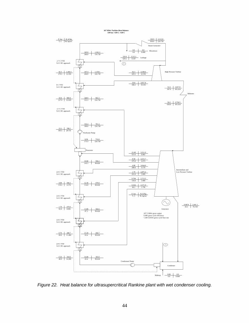
44



Steam Generator

0.0 0.0345.9 1,361.3 0.0 0.000306.8 124.730

329.9 3,512.1629.2 0.187




347.9 101.614

Reheater

50.8 980.8 348.9 965.3227.9 22.929 222.3 124.730

50.2 3,736.5630.0 101.614


350.4 781.4180.0 124.730

23.5 788.2185.5 29.731

Feedwater Pump

8.58 733.8173.3 124.730

Deaerator23.49 3,511.0521.0 6.802

8.58 3,215.710.80 596.2 375.9 4.373141.5 90.626

4.08 3,044.0288.8 4.176


0.704 2,713.3116.8 3.400

4.08 596.2 12.30 479.0119.5 4.176 114.0 90.626 0.264 2,571.9

66.2 2.796


0.0874 2,441.11.79 479.0 43.2 76.15892.8 8.085 13.80 366.6 Generator



0.70 288.7 15.30 266.769.0 11.484 63.4 90.626


0.26 204.8 16.80 183.048.9 14.280 43.4 90.626

Condensate Pump

Condenser

0.00 0.00.0 0.000

1

1

Blowdown

Leakage

Makeup

Figure 22. Heat balance for ultrasupercritical Rankine plant with wet condenser cooling.

45



Steam Generator

0.0 0.0345.9 1,361.3 0.0 0.000306.8 124.700

329.9 3,512.1629.2 0.000




347.9 101.776

Reheater

50.8 980.8 348.9 965.3227.9 22.924 222.3 124.700

50.2 3,736.5630.0 101.776


350.4 781.4180.0 124.700

23.5 788.2185.5 29.724

Feedwater Pump

8.58 733.8173.3 124.700

Deaerator23.49 3,511.0521.0 6.801

8.58 3,215.710.80 596.2 375.9 4.372141.5 90.603

4.08 3,041.3287.5 4.179


0.704 2,708.7114.5 3.405

4.08 596.2 12.30 479.0119.5 4.179 114.0 90.603 0.264 2,566.5

66.2 1.118


0.1724 2,518.81.79 479.0 56.9 77.98692.8 8.094 13.80 366.6 Generator



0.70 288.7 15.30 266.769.0 11.499 63.4 90.603


0.26 255.8 16.80 234.061.1 12.617 55.6 90.603

Condensate Pump

Condenser

0.00 0.00.0 0.000

1

1

Blowdown

Leakage

Makeup Figure 23. Heat balance for ultrasupercritical Rankine plant with dry condenser cooling.

46

47

Chapter 3 Performance Analysis

This chapter begins by describing the computer code used to estimate the annual energy of the plant designs described in Chapter 2. This is followed, in subsequent sections, by discussions of the development of the input parameters to the code and the results of the analysis. 3.1 Overview of the SOLERGY Computer Code The SOLERGY computer code [46] was used to predict the annual energy production of the power plant designs. This code was selected because it was shown to give a realistic estimate of the actual energy produced by the Solar One and Solar Two plants [12, 13]. SOLERGY simulates the operation of a solar central receiver power plant using an insolation record recorded at 15-minute intervals. The relatively short intervals are needed to model plant startup and the effects of cloud transients. The code has subroutines for each major plant system, i.e., heliostat field, receiver, thermal-energy storage, and turbine/generator. A program flow diagram is shown in Figure 24. For each 15-minute time step, SOLERGY determines the plant’s operational state (shutdown, starting up, etc.) and calculates steady-state power flows through each plant system. Annual plant performance is found by summing the performance at every 15-minute time step. SOLERGY’s computational algorithms are based on simple conservation of energy. There are no detailed thermodynamic calculations—no tracking of pressures and temperatures throughout the plant. Detailed calculations are necessary for the design and analysis of the performance over short periods but are not practical for an analysis of annual energy performance. Such calculations, however, are an important source of the data used as input to SOLERGY. In SOLERGY, user-specified plant operational parameters are used to determine the plant’s operation and performance during each time step. Examples of these parameters are (1) the time or energy required to start up and operate a system, (2) the parasitic load of major components and/or systems, and (3) the performance of individual components (e.g., receiver thermal losses or turbine efficiency). Parameters are typically estimated from hand-done calculations or obtained by running complex computer codes outside of SOLERGY. In some cases, data from tests performed at SNL or Solar One/Two can be used to estimate the code input parameters. The versions of SOLERGY used in this study are somewhat different than the original version documented in Reference 46. Improvements in the modeling of parasitic power consumption, system behavior during short-term cloud transients, and dry-condenser cooling constitute the most important differences. These improvements are described later in this chapter.

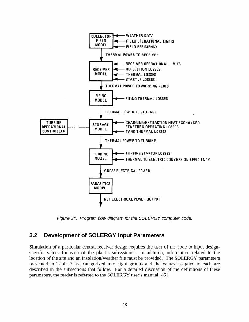
48

Figure 24. Program flow diagram for the SOLERGY computer code. 3.2 Development of SOLERGY Input Parameters Simulation of a particular central receiver design requires the user of the code to input design-specific values for each of the plant’s subsystems. In addition, information related to the location of the site and an insolation/weather file must be provided. The SOLERGY parameters presented in Table 7 are categorized into eight groups and the values assigned to each are described in the subsections that follow. For a detailed discussion of the definitions of these parameters, the reader is referred to the SOLERGY user’s manual [46].

49

Site Parameters The power plants are assumed to be located near the Solar One/Two site in Barstow, California. This site was selected because it has good insolation characteristics and an abundance of weather data exist. For example, the 30-year average value of direct-normal insolation in Barstow (Daggett) was estimated to be 2.74 MWhr/m2/yr [47]. The 15-minute weather file used in this study was measured in 1977 at Barstow by Aerospace Corporation; total annual direct normal irradiation (DNI) was 2.71 MWhr/m2/yr [48]. Parameters for the Heliostat Field This group addresses the availability and performance of the heliostats in the collector field. As described in Chapter 2, the field sizes for the subcritical, supercritical, and ultra-supercritical plants were calculated by the DELSOL3 computer code [10]. DELSOL3 was also used to determine field efficiency as a function of sun position. The results of these DELSOL calculations are presented in Tables 8 through 10. These efficiencies include optical losses due to heliostat reflectance, cosine effects, heliostat shading and blocking, atmospheric transmission, receiver interception, and receiver absorptance. When running DELSOL a flux constrained aiming strategy for the heliostats was employed such that peak flux on the receiver was limited to ~1 MW/m2 (1000 suns). This value is somewhat larger than the 800-sun limit adopted at Solar Two but is predicted to be acceptable using advanced receiver materials (see discussion in Section 2.2). As described in Chapter 2, all plants are assumed to use glass/metal heliostats similar to the 95 m2 Generation-3 version made by ATS in the 1980s (see Figure 4). The clean reflectance for this type of heliostat was measured to be 94% when new [49] and has not degraded significantly in more than 20 years of outdoor, face-up exposure at the National Solar Thermal Test Facility (NSTTF). The reflectivity values presented in Table 7 are the product of the clean reflectance and a cleanliness factor of 95%. The latter value was obtained from experience at trough power plants that suggests that regular mirror washing can achieve an annual-average cleanliness of 95% [50].

50

Table 7. SOLERGY Input Parameters for Subcritical (Sub), Supercritical (SC), and Ultra-Supercritical (USC) Rankine Plants.

Parameter Description Sub SC USC

Site Parameters SOLWEA Insolation/weather file 1977 Barstow, 2.707 MWh/m2 ALAT Local latitude (degrees) 34.9 34.9 34.9 ALONG Local longitude (degrees) 117.0 117.0 117.0 ZONE Local international time zone Pacific Pacific Pacific

Parameters for Heliostat Field FS Heliostat field reflective area (m2) 1901157 1926548 1948216 ELIM Minimum sun elevation angle for

heliostat field operation (degrees)

RFLCTY Heliostat reflectivity (included in Tables 8 to 10)

0.893 0.893 0.893

Heliostat availability 0.99 0.99 0.99 FR Field efficiency matrix Tab 8 Tab 9 Tab 10 WSLIM Wind stow speed (m/s) 17.9 17.9 17.9

Parameters for Receiver System EPS Receiver absorptance

(included in Tables 8 to 10) 0.94 0.94 0.94

RS Receiver thermal rating (MWt) 1000.0 1000.0 1000.0 ALPHAR Receiver cooldown parameter (hrs-1) 0.2 0.2 0.2 TREQD Time delay for receiver startup (hrs) 0.75 0.75 0.75 RMF Receiver minimum flow fraction 0.16 0.16 0.16 PLXLR Receiver thermal losses, hot (MWt)

vs. wind speed 55.5 66.6 74.9

PA(26) Receiver thermal losses, standby (MWt) 16.7 16.7 16.7 EXFAC Fraction of clear-sky insolation that is

unusable (if=0, all DNI is usable) 0 0 0

Parameters for Thermal Storage System PTSMAX Maximum charging rate (MWt) 1000.0 1000.0 1000.0 PFSMAX Maximum discharge rate (MWt) 337.5 337.5 337.5 EMAX Maximum value of storage (MWthr) 5000.0 5000.0 5000.0 EMIN Minimum value of storage (MWthr) 0 0 0 TNKLF Heat loss from storage system (MWt) 1.0 1.05 1.05 DLF Heat loss from steam generator (MWt) 1.0 1.0 1.0

Parameters for Steam Turbine System TBHWS Time between hot and warm start (hr) 12 12 12 TBHWS Time between warm and cold start (hr) 60 60 69 SDH Hot turbine sync delay (hr) 0.25 0.25 0.25

51

Table 7. SOLERGY Input Parameters for Subcritical (Sub),

Supercritical (SC), and Ultra-Supercritical (USC) Rankine Plants

Parameter Description Sub SC USC SDW Warm turbine sync delay (hr) 1.0 1.0 1.0 SDC Cold turbine sync delay (hr) 1.8 1.8 1.8 RDH Hot turbine ramp delay (hr) 0.4 0.4 0.4 RDW Warm turbine ramp delay (hr) 1.7 1.7 1.7 RDC Cold turbine ramp delay (hr) 2.7 2.7 2.7 TPFSL Thermal power for rated turbine

operation (MWt) 337.5 337.5 337.5

TMFS Minimum turbine flow fraction 0.3 0.3 0.3 ESMIN1 Minimum storage level for turbine

start, receiver operating (MWthr) 200.0 200.0 200.0

ESMIN2 Minimum storage level for turbine start, receiver not operating (MWthr)

337.5 337.5 337.5

ESMAX1 Storage level at which turbine must be started, receiver operating (MWthr)

200.0 200.0 200.0

TSTDR Time to startup steam generator (hr) (included startup in TMFS and SDX)

0. 0. 0.

FEPSS Turbine thermal-to-electric efficiency Tab 11 Tab 12 Tab 13 REPSS vs. fraction of rated power CEPSS vs. temperature (oF)

Piping Parameters YXLP Piping loss coefficients TXLP vs. ambient temperature ( /oF) 3.4e-4/-4. Same 3.2e-4/32. 3.2e-4/50. 3.0e-4/86. 2.8e-4/122.

Parameters for Steam Generator DLF Steam generator heat losses (MWt) 1.0 1.0 1.0 REFPC Reference power for steam generator

thermal losses (MWt) 337.5 337.5 337.5

PWARMD Maximum heat to steam generator during startup (MWt)

30.0 30.0 30.0

Parameters for Electrical Parasitics PA(1) Power to run heliostat field (MWe/m2) 5.22e-7 5.22e-7 5.22e-7 PA(2) Power to stow/unstow heliostat field

during 0.25 hr interval (MWe /m2)

PA(3)-PA(5) Cold salt pump curve-fit parameters Fig 26 Fig 26 Fig 26 PA(7)-PA(8) Turbine plant curve-fit parameters Tab 11 Tab 12 Tab 13

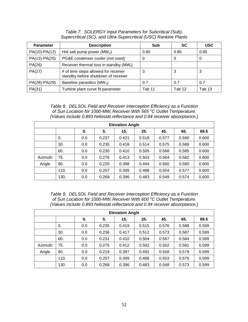
52

Table 7. SOLERGY Input Parameters for Subcritical (Sub), Supercritical (SC), and Ultra-Supercritical (USC) Rankine Plants

Parameter Description Sub SC USC PA(10)-PA(12) Hot salt pump power (MWe) 0.85 0.85 0.85 PA(13)-PA(25) PG&E condenser cooler (not used) 0 0 0 PA(26) Receiver thermal loss in standby (MWt) PA(27) # of time steps allowed for receiver

standby before shutdown of receiver 3 3 3

PA(28)-PA(29) Baseline parasitics (MWe) 0.7 0.7 0.7 PA(31) Turbine plant curve fit parameter Tab 11 Tab 12 Tab 13

Table 8. DELSOL Field and Receiver Interception Efficiency as a Function of Sun Location for 1000-MWt Receiver With 565 oC Outlet Temperature.

(Values include 0.893 heliostat reflectance and 0.94 receiver absorptance.)

Elevation Angle 0. 5. 15. 25. 45. 65. 89.5 0. 0.0 0.237 0.421 0.518 0.577 0.590 0.600 30. 0.0 0.235 0.418 0.514 0.575 0.588 0.600 60. 0.0 0.230 0.410 0.505 0.568 0.585 0.600

Azimuth 75. 0.0 0.276 0.413 0.503 0.564 0.582 0.600 Angle 90. 0.0 0.220 0.398 0.494 0.560 0.580 0.600

110. 0.0 0.257 0.399 0.488 0.554 0.577 0.600 130. 0.0 0.269 0.396 0.483 0.549 0.574 0.600



Elevation Angle 0. 5. 15. 25. 45. 65. 89.5 0. 0.0 0.235 0.419 0.515 0.576 0.588 0.599 30. 0.0 0.236 0.417 0.512 0.573 0.587 0.599 60. 0.0 0.231 0.410 0.504 0.567 0.584 0.599

Azimuth 75. 0.0 0.275 0.412 0.502 0.562 0.581 0.599 Angle 90. 0.0 0.219 0.397 0.492 0.558 0.579 0.599

110. 0.0 0.257 0.399 0.488 0.553 0.576 0.599 130. 0.0 0.268 0.396 0.483 0.548 0.573 0.599

53



Elevation Angle 0. 5. 15. 25. 45. 65. 89.5 0. 0.0 0.235 0.417 0.513 0.573 0.587 0.599 30. 0.0 0.236 0.415 0.510 0.571 0.586 0.599 60. 0.0 0.230 0.408 0.503 0.565 0.583 0.599

Azimuth 75. 0.0 0.275 0.412 0.501 0.561 0.580 0.598 Angle 90. 0.0 0.222 0.398 0.493 0.558 0.578 0.598

110. 0.0 0.259 0.400 0.489 0.553 0.575 0.598 130. 0.0 0.268 0.397 0.484 0.549 0.573 0.598

The value for heliostat availability was selected to be 99%. This value is supported by reliability data collected for the Solar One heliostat field [51]. The collector field startup angle is also supported by experience at Solar One/Two; the heliostats were typically tracking the receiver at sunrise. Parameters for the Receiver System This group of parameters addresses the performance of the receiver during startup, shutdown, and steady-state operation. The receiver thermal ratings are assumed to be 1000 MWt. The Utility Studies [2] investigated salt receivers with thermal ratings of ~500 MWt

19 and ~1000 MWt and a solar plant using the larger receiver was predicted to result in a lower LCOE. Another reason for selecting 1000 MW is due to the belief by SNL that supercritical Rankine plants will likely need to provide Baseload energy with power ratings of ~160 MWe (as described in Section 2.4). Given a conversion efficiency of 48%, this Rankine plant would require 160/0.48 = 333 MW of thermal energy. Studies have shown (e.g., see Reference 6) that a molten-salt plant with a solar multiple of 3 combined with 15 hours of thermal storage yields the lowest LCOE for a given turbine size and achieves a solar-only capacity factor of 70 to 75%20 for a plant installed in the Southwestern deserts. Thus, the receiver should be 3*333 or ~1000 MWt. Receiver absorptance was estimated by taking the average of possible best-case and worst-case values. The best case would be the value achieved at Solar One, i.e., 95%. This value was maintained during the final 2.5 years of its operation. The average absorptance for a molten-salt receiver could be somewhat lower than the receiver at Solar One, even though the tubes of both receivers are coated with the same Pyromark paint. This is because the paint on a salt receiver is exposed to a harsher environment; solar flux and temperatures are higher and any salt leakage

19 The salt receiver currently being promoted by SolarReserve is ~500 MWt. 20 If capacity factors greater than 70% are required, a small amount of fossil backup might be used to achieve a

typical baseload capacity factor of >80%.

54

will rapidly degrade the paint near the hole in the tube. It was therefore judged that in the worst case the average absorptance could be 93%, even with regular repainting of the receiver every few years. The minimum flow at which the receiver can operate, 16%, was measured during testing of a 5-MWt salt receiver at SNL during 1988 [23]; values between 15 and 20% were also demonstrated at Solar Two [13]. Thermal losses from the Solar Two receiver were measured to be between 2.7 and 3 MWt over a range of wind speeds [15]. Since the absorber surface area was 99 m2, the loss was ~30 kWt/m2. This value was used to estimate the thermal losses for the receiver in the subcritical plant with the same 285/565 oC salt inlet/exit temperatures as Solar Two. For the higher-temperature receivers in the supercritical plants, the receiver thermal model described in Section 2.2 was calibrated with the Solar Two data and used to calculate the increased thermal losses given a 600 or 650 oC outlet temperature, estimated to be 36 and 40 kWt/m2, respectively. When the receiver is in standby with no sun on it, the outlet temperature will drop to a few degrees below the inlet temperature. The receiver model predicts ~9 kWt/m2 with the receiver in standby. Standby can occur during startup of the receiver and while waiting for cloudy weather to clear. It was assumed the operators would maintain the receiver in cloud standby for 0.75 hours before shutting it down and draining it. Receiver startup in the morning and restart following cloud-induced shutdowns is simulated by selecting proper values for the SOLERGY parameters TREQD and ALPHAR. Experimentation with SOLERGY found the values listed in Table 7 to produce reasonable results; the salt receiver completed start up 1.25 hours after sunrise and returned to rated conditions 0.25 hours after a cloud shutdown. This matches experimental data recorded during the test of the 5-MWt salt receiver at SNL [23] and at Solar Two. (Typically, 0.5 hours is required to achieve minimum flow, followed by 0.75 hours of startup for a total of 1.25 hours to rated condition after sunrise.) When SOLERGY was validated with Solar One data it was found that use of 15-minute-average insolation data, rather than more frequent 3-minute data, led to an overprediciton of plant performance on days when large and frequent opaque clouds were passing over the heliostat field [12]. Since Solar One used a steam receiver that was powered by a relatively small heliostat field, this type of weather quickly caused the steam conditions in the receiver to degrade below the trip setpoint of the turbine. When the sun returned there was a significant amount of time when solar energy was not converted to electricity while the operators restarted the receiver and turbine. These short-term transients and corresponding energy losses were not captured by SOLERGY with 15-minute insolation data; however, they were captured when 3-minute data were used. Typical insolation data files have time steps of 15-minute or longer. SOLERGY was therefore improved to model the concept of “useful insolation.” The amount that is “useful” is a function of the time constant and trip setpoints of the solar plant, as well as the DNI time-step. The parameter EXFAC is used to capture these features associated with the plant design, as well as the weather file. The new SOLERGY model compares the DNI for a particular time step in the weather file with a value that would occur if the sky was totally clear and calculates a ratio of the 2 values. If the actual DNI is less than X% of clear sky value, SOLERGY will trip the receiver and force a restart at a later time step when the clouds clear the field. For example, it

55

was found that a value of 60% greatly improved the SOLERGY prediction of Solar One performance on partly cloudy days when 15-minute DNI data were used. All this being said, the value of EXFAC chosen for a molten-salt plant was set to zero, implying that all DNI in the 15-minute weather file is considered useful. Experience at Solar Two indicated that, unlike Solar One, the receiver and turbine could continue to operate through partly cloudy weather; since there was a storage tank between the turbine and receiver, clouds did not quickly lead to turbine trip. Parameters for the Thermal Storage System The maximum charging rate of the salt-storage system (PTSMAX) was set equal to the maximum power of the receiver, and the maximum discharge rate (PFSMAX) was set equal to the thermal power demands of the steam-generator system. A sun-following dispatch strategy of stored energy within the tanks was chosen. 21 This minimizes the size of the tanks because the stored energy is held for the minimum amount of time before being discharged to the steam generator. The size of the storage tanks was chosen to operate the turbine for 15 hours. Given a solar multiple of 3, approximately 15 hours of storage has been shown to result in the lowest LCOE [6]. Since the receiver is 1000 MWt, a solar multiple of 3 results in a steam generator with a 333-MWt rating.22 Fifteen hours of storage is thus 15 * 333 ~ 5000 MWht. This size is the value for EMAX in Table 7. The heat loss from the hot and cold tanks for the 5000-MWh system was based on a heat loss calculation performed by Chicago Bridge and Iron for a hypothetical commercial-scale system [53]. In that study, the heat loss for the hot tank within a 1560-MWh system was estimated to be 244 kW. Thermal losses from the cold tank were not given, but can be estimated by assuming the same overall heat transfer coefficient (UA). Assuming an ambient temperature of 25 oC, the value for the hot tank is estimated from UA = Q/ΔT = (244/(565-25)) = 0.45 kW/oC. The cold tank losses would therefore be Q = 0.45*(288-25) = 118 kWt. Total hot and cold tank thermal losses are therefore 362 kWt for the 1560-MWh system. Since the 5000 MWh is roughly three times larger, the total thermal losses are also assumed to be 3 times larger, or ~1 MWt. Parameters for the Steam-Turbine System This group of parameters addresses the performance of the turbine generators during startup and steady-state operation. The startup parameters were taken from the SOLERGY model developed by Bechtel National, Inc., for the US Utility Study [2]. This subcritical turbine was made by General Electric (GE) and was first proposed for use in the Solar 100 study [54]. The parameters were assumed to be the same for the supercritical turbines. 21 SOLERGY can also be run to maximize revenue according to a “time-of-day” electricity pricing schedule. The

optimum amount of storage given time-of-day pricing would be different than a “sun-following” dispatch strategy. See References 46 and 52.

22 The analysis was actually based on a value of 337 MWt.

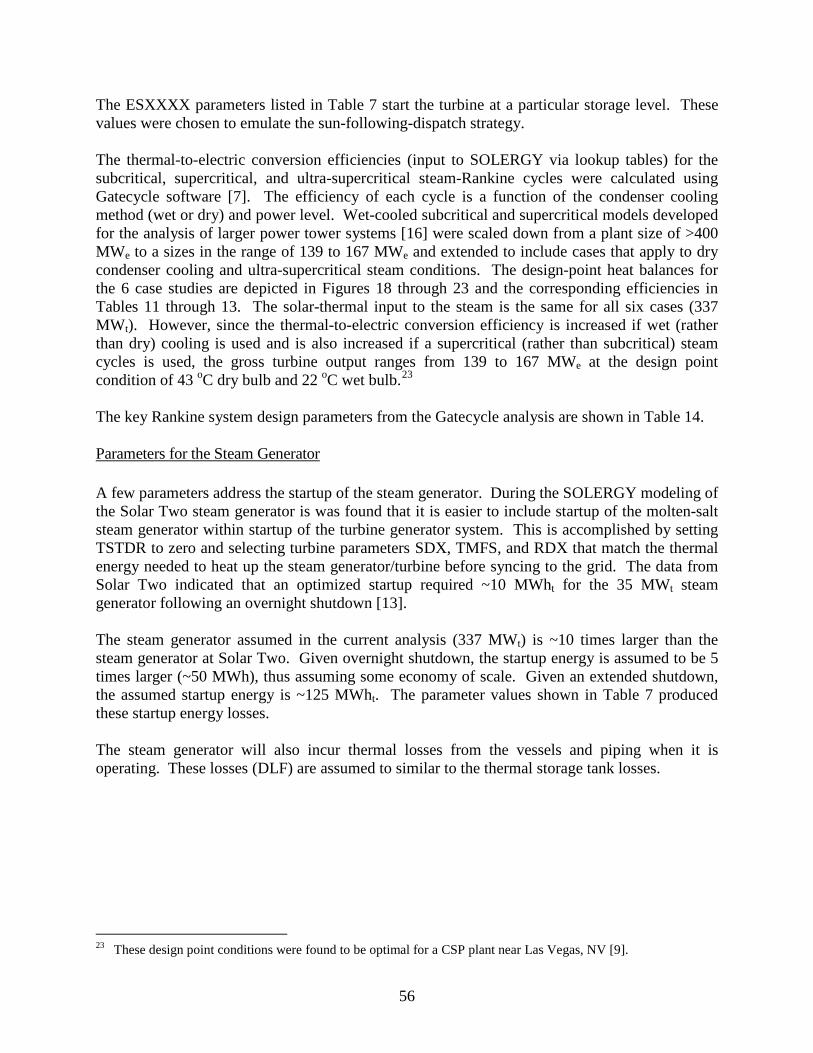
56

The ESXXXX parameters listed in Table 7 start the turbine at a particular storage level. These values were chosen to emulate the sun-following-dispatch strategy. The thermal-to-electric conversion efficiencies (input to SOLERGY via lookup tables) for the subcritical, supercritical, and ultra-supercritical steam-Rankine cycles were calculated using Gatecycle software [7]. The efficiency of each cycle is a function of the condenser cooling method (wet or dry) and power level. Wet-cooled subcritical and supercritical models developed for the analysis of larger power tower systems [16] were scaled down from a plant size of >400 MWe to a sizes in the range of 139 to 167 MWe and extended to include cases that apply to dry condenser cooling and ultra-supercritical steam conditions. The design-point heat balances for the 6 case studies are depicted in Figures 18 through 23 and the corresponding efficiencies in Tables 11 through 13. The solar-thermal input to the steam is the same for all six cases (337 MWt). However, since the thermal-to-electric conversion efficiency is increased if wet (rather than dry) cooling is used and is also increased if a supercritical (rather than subcritical) steam cycles is used, the gross turbine output ranges from 139 to 167 MWe at the design point condition of 43 oC dry bulb and 22 oC wet bulb.23 The key Rankine system design parameters from the Gatecycle analysis are shown in Table 14. Parameters for the Steam Generator A few parameters address the startup of the steam generator. During the SOLERGY modeling of the Solar Two steam generator is was found that it is easier to include startup of the molten-salt steam generator within startup of the turbine generator system. This is accomplished by setting TSTDR to zero and selecting turbine parameters SDX, TMFS, and RDX that match the thermal energy needed to heat up the steam generator/turbine before syncing to the grid. The data from Solar Two indicated that an optimized startup required ~10 MWht for the 35 MWt steam generator following an overnight shutdown [13]. The steam generator assumed in the current analysis (337 MWt) is ~10 times larger than the steam generator at Solar Two. Given overnight shutdown, the startup energy is assumed to be 5 times larger (~50 MWh), thus assuming some economy of scale. Given an extended shutdown, the assumed startup energy is ~125 MWht. The parameter values shown in Table 7 produced these startup energy losses. The steam generator will also incur thermal losses from the vessels and piping when it is operating. These losses (DLF) are assumed to similar to the thermal storage tank losses.

23 These design point conditions were found to be optimal for a CSP plant near Las Vegas, NV [9].

57

Table 11. GateCycle Prediction of Gross Rankine

Cycle Efficiency and Parasitics for Subcritical Steam Plants. (Designed at 43 oC (109 oF) Dry Bulb, 22 oC (72 oF) Wet Bulb.)

Wet-Cooled Condenser (43.0% η @DP)

Wet Bulb Power

50% 70% 100% 20 oF 42.7% η

585 FWP 78 CP

1142 CTF 744 CWP

2549 kW Total

43.1% η 1015 FWP

90 CP 1106 CTF 744 CWP

2955 kW Total

43.6% η 2140 FWP

116 CP 1058 CTF 745 CWP

4058 kW Total 40 oF 42.7% η 43.1% η 43.6% η 60 oF 42.2% η 42.8% η 43.4% η 80 oF 40.6% η

585 FWP 78 CP

1095 CTF 747 CWP

2506 kW Total

41.8% η 1015 FWP

90 CP 1075 CTF 747 CWP

2927 kW Total

42.6% η 2140 FWP

116 CP 1045 CTF 748 CWP

4048 kW Total

Dry-Cooled Condenser (41.2% η @DP)

Dry Bulb Power

50% 70% 100% 30 oF 41.1% η

585 FWP 78 CP

1229 CTF 1892 kW Total

41.5% η 1015 FWP

90 CP 1229 CTF

2333 kW Total

41.7% η 2140 FWP

114 CP 1229 CTF

3483 kW Total 60 oF 40.9% η

585 FWP 78 CP


41.3% η 1015 FWP

90 CP 1555 CTF

2660 kW Total

41.9% η 2140 FWP

114 CP 1944 CTF

4198 kW Total 90 oF 40.3% η

585 FWP 78 CP


41.0% η 1015 FWP

89 CP 2584 CTF

3688 kW Total

41.7% η 2140 FWP

114 CP 2953 CTF

5207 kW Total 120 oF 37.5% η

585 FWP 78 CP


39.0% η 1015 FWP

89 CP 3497 CTF

4600 kW Total

40.2% η 2140 FWP

113 CP 3497 CTF

5750 kW Total

FWP (Feed Pump), CP (Condensate Pump), CTF (Tower Fans), CWP (Circ Water Pump)

58

Table 12. GateCycle Prediction of Gross Rankine Cycle Efficiency and Parasitics for Supercritical Steam Plants. (Designed at 43 oC (109 oF) Dry Bulb, 22 oC (72 oF) Wet Bulb.)


Wet Bulb Power

50% 70% 100% 20 oF 47.1% η 48.0% η 49.1% η 40 oF 47.1% η 48.0% η 49.0% η 60 oF 46.6% η

2441 FWP 99 CP

1232 CTF 773 CWP

4545 kW Total

47.6% η 3620 FWP

138 CP 1208 CTF 773 CWP

5739 kW Total

48.8% η 5705 FWP

198 CP 1174 CTF 774 CWP

7851 kW Total 80 oF 44.9% η 46.4% η 47.9% η


Dry Bulb Power

50% 70% 100% 30 oF 45.7% η

2441 FWP 98 CP


46.6% η 3620 FWP

138 CP 1161 CTF

4918 kW Total

47.6% η 5709 FWP

198 CP 1355 CTF

7262 kW Total 60 oF 45.6% η

2441 FWP 98 CP


46.5% η 3619 FWP

138 CP 1650 CTF

5407 kW Total

47.6% η 5710 FWP

199 CP 1833 CTF

7741 kW Total 90 oF 44.8% η

2441 FWP 99 CP


46.2% η 3619 FWP

138 CP 2773 CTF

6530 kW Total

47.5% η 5710 FWP

199 CP 3120 CTF

9028 kW Total 120 oF 42.0% η

2441 FWP 99 CP


43.9% η 3620 FWP

138 CP 3253 CTF

7010 kW Total

45.8% η 5709 FWP

199 CP 3253 CTF

9161 kW Total


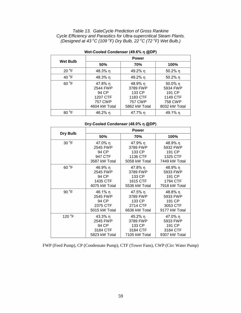
59

Table 13. GateCycle Prediction of Gross Rankine Cycle Efficiency and Parasitics for Ultra-supercritical Steam Plants.

(Designed at 43 oC (109 oF) Dry Bulb, 22 oC (72 oF) Wet Bulb.)


Wet Bulb Power

50% 70% 100% 20 oF 48.3% η 49.2% η 50.2% η 40 oF 48.3% η 49.2% η 50.2% η 60 oF 47.8% η

2544 FWP 94 CP

1207 CTF 757 CWP

4604 kW Total

48.9% η 3789 FWP

133 CP 1183 CTF 757 CWP

5862 kW Total

50.0% η 5934 FWP

191 CP 1149 CTF 758 CWP

8032 kW Total 80 oF 46.2% η 47.7% η 49.1% η


Dry Bulb Power

50% 70% 100% 30 oF 47.0% η

2545 FWP 94 CP


47.9% η 3789 FWP

133 CP 1136 CTF

5058 kW Total

48.9% η 5932 FWP

191 CP 1325 CTF

7449 kW Total 60 oF 46.9% η

2545 FWP 94 CP


47.8% η 3789 FWP

133 CP 1615 CTF

5536 kW Total

48.9% η 5933 FWP

191 CP 1794 CTF

7918 kW Total 90 oF 46.1% η

2545 FWP 94 CP


47.5% η 3789 FWP

133 CP 2714 CTF

6636 kW Total

48.8% η 5933 FWP

191 CP 3053 CTF

9177 kW Total 120 oF 43.3% η

2545 FWP 94 CP


45.2% η 3789 FWP

133 CP 3184 CTF

7105 kW Total

47.0% η 5933 FWP

191 CP 3184 CTF

9307 kW Total


60

Table 14. GateCycle Rankine Plant Design Parameters.

SUB SC USC Wet Dry Wet Dry Wet Dry

LP turbine exhaust area (m2) 3.3 1.9 3.2 1.9 3.1 1.9

FW heater areas (m2) 296 296 624 624 550 550 (top to bottom on heat balance diagram) 432 432 682 682 603 603 217 215 532 532 476 476 276 274 256 256 235 235 260 178 287 288 265 266 299 299 284 285 275 162 264 156

Steam generator duties (MWt) Preheater 58 58 Evaporator 135 135 269 269 268 268 Superheater 90 90 Reheater 54 54 68 68 69 69 Total 337 337 337 337 337 337

Steam generator areas (m2)24 Preheater 1533 1533 Evaporator 2229 2229 Superheater 1444 1444 Reheater 1510 1510

Condenser saturation pressure (bar) 0.087 0.17 0.087 0.17 0.087 0.17

Condenser cooling system Cooling tower air-side ΔP (mbar) 2.1 1.5 2.1 1.5 2.1 1.5 Number of dry-cooling bays 24 22 22 Initial Temperature Difference (oC) 14 14 14 OD surface area (x103 m2) 20 18.7 18.4 OD+Fin surface area (x103 m2) 592 552 542

24 The molten salt heat transfer areas were estimated by software developed by Abengoa Solar [16]. See Chapter 2.

61

Piping Parameters The piping model parameters in SOLERGY define the energy lost from the receiver riser and downwcomer as a function of ambient temperature. The values presented in the table are the SOLERGY defaults. The model predicts ~0.3 MWt of thermal loss during times when the receiver is operating. Parameters for Electrical Parasitics This group of parameters addresses the electrical power used by plant auxiliaries (pumps, fans, trace heaters, etc.) during various modes of plant operation and shutdown. This electrical energy is subtracted from the gross electricity produced by the turbine generator during the calendar year to yield the net electrical output of the plant. The electric power to track and stow the heliostats was estimated by the manufacturer ATS [55], and checked with experience at Solar One [12]. Like Solar Two, variable speed pumps are used to pump the salt up the tower and through the receiver. The receivers were designed to have the same delta P as Solar Two (165 psi at full flow) with the inlet tank set to 250 psi.25 The total head requirements for the cold salt pumps are expressed by the following equation [56]: Htotal = Hstatic + Hfull (Wx%/Wfull)2 (12) where Htotal = Total head (ft),26 Hstatic = Static head (ft) = tower height + receiver height, Hfull = Friction head loss across the receiver at full pump flow (ft), and (Wx%/Wfull) = Fraction of full flow. The power consumed by the pumps can be estimated from the traditional fluid mechanics: P = W * H/η. Given operation of a single 100% capacity pump (with the redundant pump idle), the specific equation used was EP = [W1pump * Htotal]/[ηpump * ηmotor * ηvarsp * fac] (13)

25 The receiver inlet tank contains a pressurized inventory of salt that passively discharges to protect the receiver

during a station blackout. The inventory cools the receiver for 1 to 2 minutes while the diesel generator starts to repower the cold salt pumps.

26 For molten salt at 288 oC (550 oF), the conversion factor from pressure to head is 0.833 psi per foot.

62

where EP = electric power for one 100% capacity pump (kW), W1pump = flow rate of 1 pump (lb/sec), ηpump = pump efficiency as a function of flow rate and head (Figure 25), ηmotor = pump motor efficiency (0.95), ηvarsp = efficiency of variable speed coupler (0.95), and fac= =units conversion factor (737.) to yield kW when pump flow is in lb/sec and head is in ft. Plots of Equation (13) for the cold-salt pumps are presented in Figure 26, along with the curve fit equations. The turbine-plant parasitics for the three salt plants were calculated by GateCycle. By studying the results in Tables 11 through 13, the following conclusions can be drawn:

• Parasitics for the supercritical plants are higher than the subcritical plant primarily because of the higher feedwater pump parasitic; this is caused by the much higher feedwater pressure in the supercritical plants (125 bar subcritical and >300 bar for supercritical).

• Parasitics of plants with wet-cooled condensers are a weak function of wet-bulb temperature (compare 20 oF and 80 oF entries in Table 11); this dependence can be ignored. Parasitics of plants with dry-cooled condensers are a strong function of dry-bulb temperature, due to the operation of more fan bays at higher temperature.

• There is a significant variation in parasitics as a function of load.27 The parasitic results shown in Tables 11 through 13 are input to SOLERGY via curve fit relationships. The numbers in the equations are input to SOLERGY via PA(7), PA(8), and PA(31). Subcritical Wet: P = 1.0 + 3.0 * Power Level Subcritical Dry: P = 3.6395 * Power Level + 0.02645 * Dry Bulb T – 1.0404 Supercritical Wet: P = 1.2 + 6.67 * Power Level Supercritical Dry: P = 7.033 * Power Level + 0.02756 * Dry Bulb T – 0.8767 Ultrasupercritical Wet = 1.42 + 6.63 * Power Level Ultrasupercritical Dry = 7.2406 * Power Level + 0.02711 * Dry Bulb T – 0.8861 Power for the hot-salt pumps was taken from calculations performed by Babcock and Wilcox during the US Utility Study to supply salt to a U-tube, U-shell subcritical steam generator with a power rating of 260 MWt [2]. Two pumps consumed 660 kWe. Thus, for the 337 MWt steam generators analyzed here it is assumed that hot pump parasitics are (337/260)*660 = 855 kWe.

27 However, since the steam generator/turbine is operating from storage, it runs at 100% power most of the time.

Thus, part load characteristics have a second order effect on the results.

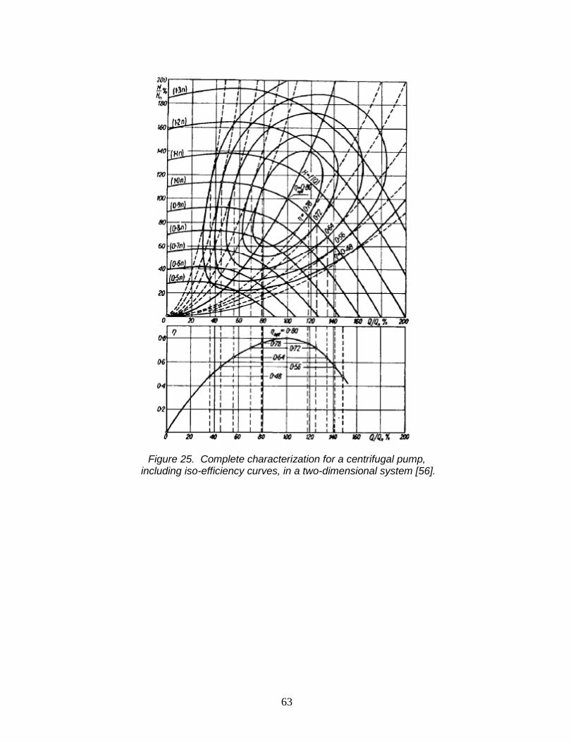
63

Figure 25. Complete characterization for a centrifugal pump,

including iso-efficiency curves, in a two-dimensional system [56].

64

Figure 26. Parasitics for the cold-salt pump as a function of flow rate. Second-order curve-fit parameters [const,W,W2] for SOLERGY are:

Sub [2.9675, 2.058, 6.6], SC [3.153, 2.09, 7.08], USC [2.785, 1.848, 6.24]. The baseline parasitics for the plants are presented in Table 15. These parasitics are assumed to occur during every hour of the year. The values were taken from Appendix B of the PG&E Utility Study [2] with a few modifications: (1) transformer losses and storage foundation cooling were added because of an apparent omission in the Utility Study and (2) plant lighting and HVAC were set to values that are consistent with the Solar One experience [12].

65

Table 15. Baseline Parasitics (MWe)

Load Sub SC USC

Turbine-Gen auxiliaries Lube oil pump Lube oil vapor extractor

36 3

Same

Collector system 8 Aux service water system 1 Storage foundation cooling 28 Secondary cooling water pump 1 Water treatment 56 Plant control system 30 Fire water jockey pump 3 Air compressor 10 Steam generator heaters 24 Small nitrate salt pipe trace heaters

183

Plant lighting 50 HVAC 100 Unidentified and overnight plant maintenance

100

Transformer losses 54 Total Baseline Parasitics 687 687 687

66

3.3 SOLERGY Analysis Results Figures 27 through 32 compare the annual energy flows calculated by SOLERGY for the six case studies. The left side of each diagram shows the calculated efficiencies for each of several categories. On the right side are the absolute values of the energy losses associated with each category. It can be noted that these calculations assumed 100% plant availability. Plant availability is calculated in Chapter 4. The category “REDIRECTED ENERGY” includes losses represented within the field-efficiency matrices (Tables 8 through 10 includes heliostat cosine, shading, blocking, reflectance, receiver interception, atmospheric transmission, and receiver absorptance), as well as heliostat unavailability and times in the weather file when field operation limits are exceeded (in this case, when high winds cause the shutdown of the heliostat field). Comparing the six case studies reveals that field efficiency is slightly worse for the supercritical plants; since receiver thermal losses are higher for the supercritical plants, additional heliostats were added by DELSOL to the southern portion of the field to compensate for this additional thermal loss and heliostats in the south field have the lowest cosine efficiency. The category “RCVR INCIDENT ENERGY” represents losses caused by defocussing of a portion of the heliostat field when the storage system is full. The efficiency of this category is nearly the same for all six case studies. The category “RECEIVER ABSORBED ENERGY” includes losses in the receiver incurred during startup and steady-state operation. The annual efficiencies for the receivers within the subcritical, supercritical, and ultrasupercritical plants are calculated to be 85.8%, 84.3%, and 83.3%, respectively. The subcritical receiver has the highest efficiency because it operates at the lowest temperature and incurs the lowest thermal losses. The category “ENERGY TO STORAGE” represents losses in the piping between the receiver and the storage system (i.e., the riser and downcomer). These losses are insignificant. The category “ENERGY TO TURBINE” includes the thermal losses from the hot and cold storage tanks as well as operation of the steam generator. The efficiency of this category is nearly the same for all six case studies.

67

PLANT SUMMARY - DAYS 1 TO 365 YEAR 1985 EFFICIENCY (MWHRS) ENERGY LOSSES I-------------------------I (MWHRS) I TOTAL INSOLATION I I 5146424.00 I I-------------------------I V I-------------------------I OUTAGE LOSSES 1.000 I AVAILABLE ENERGY I .00 (YEOUTAGE) I 5146424.00 I I-------------------------I V I-------------------------I FIELD LOSSES .990 I REDIRECTED ENERGY I 51464.19 HELIOSTAT UNAVAILABILITY LOSS .525 I 2674830.00 I 2420130.00 REFLECTANCE, COSINE,SHADOWING, BLOCKING, I-------------------------I SPILLAGE,TRANSMISION (OPERATION LIMITS=2051.30) V I-------------------------I STORAGE FULL .951 I RCVR INCIDENT ENERGY I 131497.60 DEFOCUS HELIOSTATS (YSUPTR) I 2543332.00 I I-------------------------I V I-------------------------I RECEIVER LOSSES I RECEIVER I 59211.55 RCVR MIN FLOW (YPLRMF) I ABSORBED ENERGY I 12025.50 SURPLUS ENERGY TO RCVR DEFOCUS HELIOSTATS (YSPTR) .858 I I .00 ABSORPTANCE (INCLUDED IN FIELD) I 2181052.00 I 177140.40 THERMAL LOSS (RADIATION AND CONVECTION) I-------------------------I 113902.80 RCVR STARTUP (YRSTRT) V I-------------------------I PIPING LOSSES 1.000 I ENERGY TO STORAGE I 910.25 I 2180141.00 I I-------------------------I V I-------------------------I STORAGE LOSSES I I I ENERGY TO I .993 I TURBINE* I 8760.00 TANK LOSS (YTNKLOS) I 2164816.00 I .00 STEAM GENERATOR STARTUP (INCLUDED IN TURBINE SYNC) I-------------------------I 6586.75 LOSS FROM STEAM GEN (YTPLDD) V * -21.75 MWHRS IN STORAGE AT END OF DAY 365 V I-------------------------I EPGS LOSSES .431 I GROSS ENERGY I 15778.12 TURBINE SYNC LOSS (YTSTRT) I 933282.20 I 1215754.00 RANKINE LOSS (APPROX) I-------------------------I V I-------------------------I AUXILIARY ENERGY I NET ENERGY I .922 I OUTPUT I 31516.38 TURBINE PLANT (YTPPAR) I I 34949.82 SOLAR PLANT (YSPPAR) I 860797.70 MWHe I 6018.10 BASELINE (YPMPAR) I-------------------------I .167 ( 72484.34 TOTAL AUX ENERGY (YPARN)) .167 OVERALL PLANT EFFICIENCY (TOTAL NET ELECTRICITY/ TOTAL DNI ON FIELD)

Figure 27. Annual energy flows within the subcritical plant with wet cooling as predicted by SOLERGY.

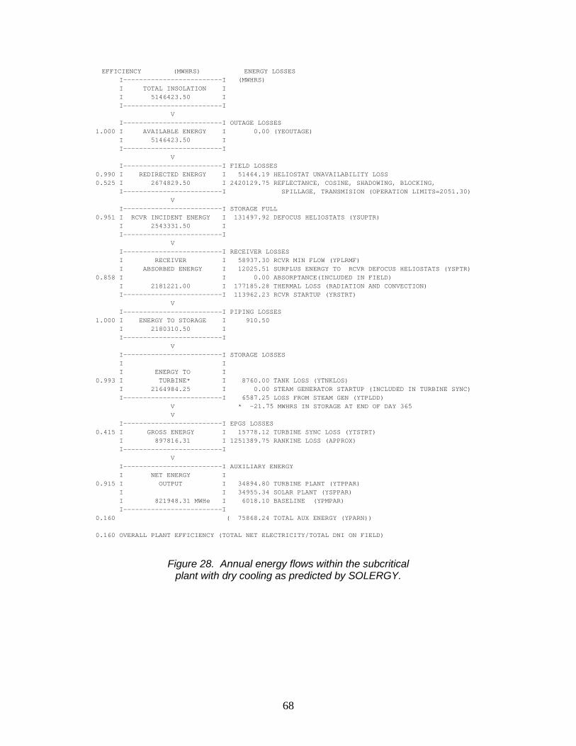
68

EFFICIENCY (MWHRS) ENERGY LOSSES I-------------------------I (MWHRS) I TOTAL INSOLATION I I 5146423.50 I I-------------------------I V I-------------------------I OUTAGE LOSSES 1.000 I AVAILABLE ENERGY I 0.00 (YEOUTAGE) I 5146423.50 I I-------------------------I V I-------------------------I FIELD LOSSES 0.990 I REDIRECTED ENERGY I 51464.19 HELIOSTAT UNAVAILABILITY LOSS 0.525 I 2674829.50 I 2420129.75 REFLECTANCE, COSINE, SHADOWING, BLOCKING, I-------------------------I SPILLAGE, TRANSMISION (OPERATION LIMITS=2051.30) V I-------------------------I STORAGE FULL 0.951 I RCVR INCIDENT ENERGY I 131497.92 DEFOCUS HELIOSTATS (YSUPTR) I 2543331.50 I I-------------------------I V I-------------------------I RECEIVER LOSSES I RECEIVER I 58937.30 RCVR MIN FLOW (YPLRMF) I ABSORBED ENERGY I 12025.51 SURPLUS ENERGY TO RCVR DEFOCUS HELIOSTATS (YSPTR) 0.858 I I 0.00 ABSORPTANCE(INCLUDED IN FIELD) I 2181221.00 I 177185.28 THERMAL LOSS (RADIATION AND CONVECTION) I-------------------------I 113962.23 RCVR STARTUP (YRSTRT) V I-------------------------I PIPING LOSSES 1.000 I ENERGY TO STORAGE I 910.50 I 2180310.50 I I-------------------------I V I-------------------------I STORAGE LOSSES I I I ENERGY TO I 0.993 I TURBINE* I 8760.00 TANK LOSS (YTNKLOS) I 2164984.25 I 0.00 STEAM GENERATOR STARTUP (INCLUDED IN TURBINE SYNC) I-------------------------I 6587.25 LOSS FROM STEAM GEN (YTPLDD) V * -21.75 MWHRS IN STORAGE AT END OF DAY 365 V I-------------------------I EPGS LOSSES 0.415 I GROSS ENERGY I 15778.12 TURBINE SYNC LOSS (YTSTRT) I 897816.31 I 1251389.75 RANKINE LOSS (APPROX) I-------------------------I V I-------------------------I AUXILIARY ENERGY I NET ENERGY I 0.915 I OUTPUT I 34894.80 TURBINE PLANT (YTPPAR) I I 34955.34 SOLAR PLANT (YSPPAR) I 821948.31 MWHe I 6018.10 BASELINE (YPMPAR) I-------------------------I 0.160 ( 75868.24 TOTAL AUX ENERGY (YPARN)) 0.160 OVERALL PLANT EFFICIENCY (TOTAL NET ELECTRICITY/TOTAL DNI ON FIELD)

Figure 28. Annual energy flows within the subcritical plant with dry cooling as predicted by SOLERGY.

69

EFFICIENCY (MWHRS) ENERGY LOSSES I-------------------------I (MWHRS) I TOTAL INSOLATION I I 5215156.00 I I-------------------------I V I-------------------------I OUTAGE LOSSES 1.000 I AVAILABLE ENERGY I .00 (YEOUTAGE) I 5215156.00 I I-------------------------I V I-------------------------I FIELD LOSSES .990 I REDIRECTED ENERGY I 52151.50 HELIOSTAT UNAVAILABILITY LOSS .524 I 2703542.00 I 2459462.00 REFLECTANCE, COSINE, SHADOWING, BLOCKING, I-------------------------I SPILLAGE, TRANSMISION (OPERATION LIMITS=2072.19) V I-------------------------I STORAGE FULL .953 I RCVR INCIDENT ENERGY I 127872.90 DEFOCUS HELIOSTATS (YSUPTR) I 2575669.00 I I-------------------------I V I-------------------------I RECEIVER LOSSES I RECEIVER I 63955.45 RCVR MIN FLOW (YPLRMF) I ABSORBED ENERGY I 12318.18 SURPLUS ENERGY TO RCVR DEFOCUS HELIOSTATS (YSPTR) .843 I I .00 ABSORPTANCE(INCLUDED IN FIELD) I 2172497.00 I 211255.30 THERMAL LOSS (RADIATION AND CONVECTION) I-------------------------I 115642.70 RCVR STARTUP (YRSTRT) V I-------------------------I PIPING LOSSES 1.000 I ENERGY TO STORAGE I 905.50 I 2171592.00 I I-------------------------I V I-------------------------I STORAGE LOSSES I I I ENERGY TO I .993 I TURBINE* I 9198.04 TANK LOSS (YTNKLOS) I 2155858.00 I .00 STEAM GENERATOR STARTUP (INCLUDED IN TURBINE SYNC) I-------------------------I 6559.00 LOSS FROM STEAM GEN (YTPLDD) V * -23.10 MWHRS IN STORAGE AT END OF DAY 365 V I-------------------------I EPGS LOSSES .484 I GROSS ENERGY I 15778.12 TURBINE SYNC LOSS (YTSTRT) I 1044489.00 I 1095590.00 RANKINE LOSS (APPROX) I-------------------------I V I-------------------------I AUXILIARY ENERGY I NET ENERGY I .905 I OUTPUT I 56270.31 TURBINE PLANT (YTPPAR) I I 36588.38 SOLAR PLANT (YSPPAR) I 945611.70 MWHe I 6018.10 BASELINE (YPMPAR) I-------------------------I .181 ( 98876.80 TOTAL AUX ENERGY (YPARN)) .181 OVERALL PLANT EFFICIENCY (TOTAL NET ELECTRICITY/ TOTAL DNI ON FIELD)

Figure 29. Annual energy flows within the supercritical plant with wet cooling as predicted by SOLERGY.

70


Figure 30. Annual energy flows within the supercritical plant with dry cooling as predicted by SOLERGY.

71

EFFICIENCY (MWHRS) ENERGY LOSSES I-------------------------I (MWHRS) I TOTAL INSOLATION I I 5273817.00 I I-------------------------I V I-------------------------I OUTAGE LOSSES 1.000 I AVAILABLE ENERGY I .00 (YEOUTAGE) I 5273817.00 I I-------------------------I V I-------------------------I FIELD LOSSES .990 I REDIRECTED ENERGY I 52738.12 HELIOSTAT UNAVAILABILITY LOSS .523 I 2728992.00 I 2492087.00 REFLECTANCE, COSINE, SHADOWING, BLOCKING, I-------------------------I SPILLAGE,TRANSMISION (OPERATION LIMITS=2089.33) V I-------------------------I STORAGE FULL .953 I RCVR INCIDENT ENERGY I 127897.40 DEFOCUS HELIOSTATS (YSUPTR) I 2601095.00 I I-------------------------I V I-------------------------I RECEIVER LOSSES I RECEIVER I 66978.60 RCVR MIN FLOW (YPLRMF) I ABSORBED ENERGY I 12878.65 SURPLUS ENERGY TO RCVR DEFOCUS HELIOSTATS (YSPTR) .833 I I .00 ABSORPTANCE(INCLUDED IN FIELD) I 2167631.00 I 236794.50 THERMAL LOSS (RADIATION AND CONVECTION) I-------------------------I 116812.00 RCVR STARTUP (YRSTRT) V I-------------------------I PIPING LOSSES 1.000 I ENERGY TO STORAGE I 902.50 I 2166729.00 I I-------------------------I V I-------------------------I STORAGE LOSSES I I I ENERGY TO I .993 I TURBINE* I 9198.04 TANK LOSS (YTNKLOS) I 2150999.00 I .00 STEAM GENERATOR STARTUP (INCLUDED IN TURBINE SYNC) I-------------------------I 6544.75 LOSS FROM STEAM GEN (YTPLDD) V * -12.52 MWHRS IN STORAGE AT END OF DAY 365 V I-------------------------I EPGS LOSSES .496 I GROSS ENERGY I 15867.46 TURBINE SYNC LOSS (YTSTRT) I 1067413.00 I 1067718.00 RANKINE LOSS (APPROX) I-------------------------I V I-------------------------I AUXILIARY ENERGY I NET ENERGY I .910 I OUTPUT I 57373.47 TURBINE PLANT (YTPPAR) I I 32798.57 SOLAR PLANT (YSPPAR) I 971222.60 MWHe I 6018.10 BASELINE (YPMPAR) I-------------------------I .184 ( 96190.09 TOTAL AUX ENERGY (YPARN)) .184 OVERALL PLANT EFFICIENCY (TOTAL NET ELECTRICITY/ TOTAL DNI ON FIELD)

Figure 31. Annual energy flows within the ultrasupercritical plant with wet cooling as predicted by SOLERGY.

72


Figure 32. Annual energy flows within the ultrasupercritical plant with dry cooling as predicted by SOLERGY.

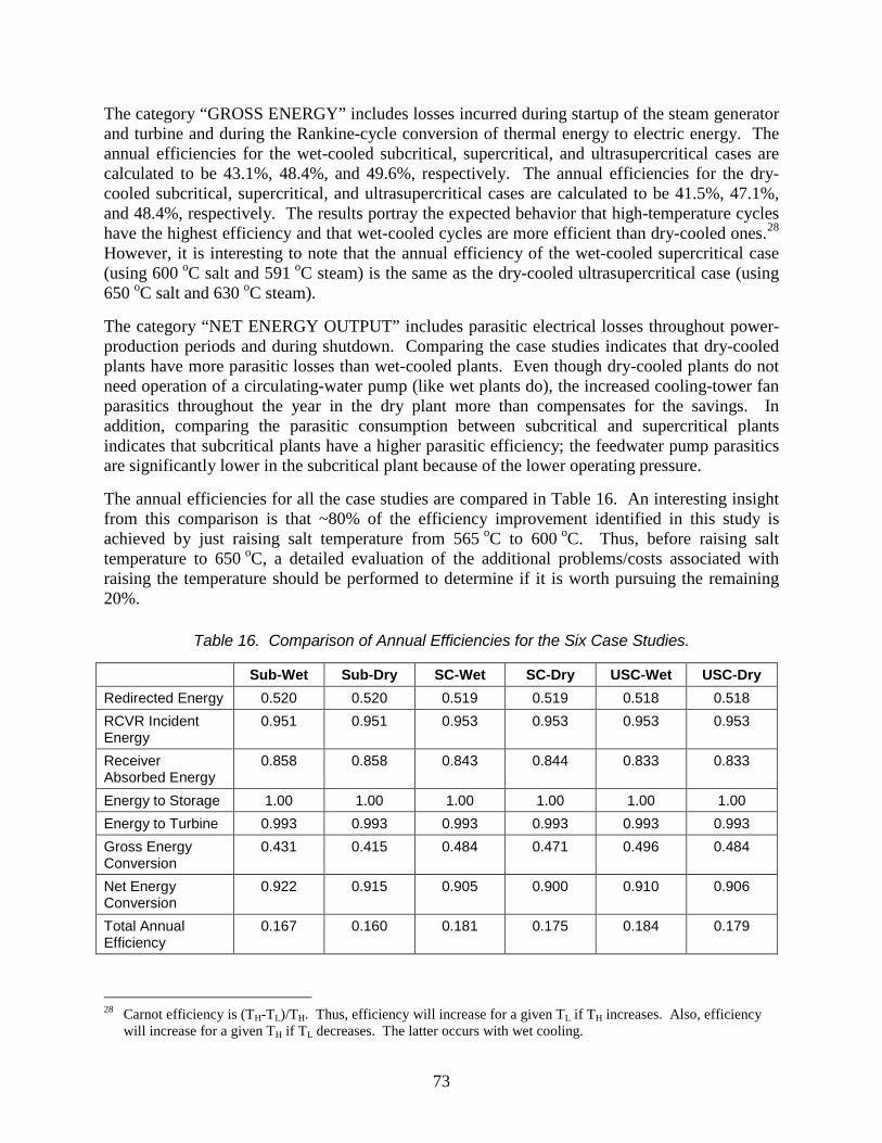
73

The category “GROSS ENERGY” includes losses incurred during startup of the steam generator and turbine and during the Rankine-cycle conversion of thermal energy to electric energy. The annual efficiencies for the wet-cooled subcritical, supercritical, and ultrasupercritical cases are calculated to be 43.1%, 48.4%, and 49.6%, respectively. The annual efficiencies for the dry-cooled subcritical, supercritical, and ultrasupercritical cases are calculated to be 41.5%, 47.1%, and 48.4%, respectively. The results portray the expected behavior that high-temperature cycles have the highest efficiency and that wet-cooled cycles are more efficient than dry-cooled ones.28 However, it is interesting to note that the annual efficiency of the wet-cooled supercritical case (using 600 oC salt and 591 oC steam) is the same as the dry-cooled ultrasupercritical case (using 650 oC salt and 630 oC steam). The category “NET ENERGY OUTPUT” includes parasitic electrical losses throughout power-production periods and during shutdown. Comparing the case studies indicates that dry-cooled plants have more parasitic losses than wet-cooled plants. Even though dry-cooled plants do not need operation of a circulating-water pump (like wet plants do), the increased cooling-tower fan parasitics throughout the year in the dry plant more than compensates for the savings. In addition, comparing the parasitic consumption between subcritical and supercritical plants indicates that subcritical plants have a higher parasitic efficiency; the feedwater pump parasitics are significantly lower in the subcritical plant because of the lower operating pressure. The annual efficiencies for all the case studies are compared in Table 16. An interesting insight from this comparison is that ~80% of the efficiency improvement identified in this study is achieved by just raising salt temperature from 565 oC to 600 oC. Thus, before raising salt temperature to 650 oC, a detailed evaluation of the additional problems/costs associated with raising the temperature should be performed to determine if it is worth pursuing the remaining 20%.

Table 16. Comparison of Annual Efficiencies for the Six Case Studies.

Sub-Wet Sub-Dry SC-Wet SC-Dry USC-Wet USC-Dry Redirected Energy 0.520 0.520 0.519 0.519 0.518 0.518 RCVR Incident Energy

0.951 0.951 0.953 0.953 0.953 0.953

Receiver Absorbed Energy

0.858 0.858 0.843 0.844 0.833 0.833

Energy to Storage 1.00 1.00 1.00 1.00 1.00 1.00 Energy to Turbine 0.993 0.993 0.993 0.993 0.993 0.993 Gross Energy Conversion

0.431 0.415 0.484 0.471 0.496 0.484

Net Energy Conversion

0.922 0.915 0.905 0.900 0.910 0.906

Total Annual Efficiency

0.167 0.160 0.181 0.175 0.184 0.179

28 Carnot efficiency is (TH-TL)/TH. Thus, efficiency will increase for a given TL if TH increases. Also, efficiency

will increase for a given TH if TL decreases. The latter occurs with wet cooling.

74

75

Chapter 4 Reliability Analysis

Equipment malfunctions will cause a solar power tower to be unavailable for power production during a certain fraction of the calendar year. In this chapter the reliability of the subcritical salt plant design is analyzed in order to estimate this unavailability fraction. Reasons for unavailability are also identified and discussed. 4.1 Overview of Pro-Opta Reliability Analysis Software SNL’s Pro-Opta software [17] was used to predict plant unavailability. As shown in Figure 33, this software has many capabilities that allow a detailed evaluation of the reliability of existing power plants as well as the optimization of proposed future plant designs. The package is currently being used to evaluate and improve the reliability of wind-turbine power plants [57]. The analysis presented in this chapter is the first time the software has been used to evaluate a solar power tower. To run the software, the analyst must provide a logic model and reliability data for the power plant components and/or subsystems. The logic model (called a “fault tree” or “reliability block diagram”) relates the series-parallel arrangement of the plant components. For example, the diagram in Figure 34 shows a series relationship between subsystems; if any of these subsystems fail, the plant becomes unavailable for power production. Two pieces of reliability data are input for each plant component: (1) the mean time between failures (MTBF), and (2) the mean downtime (MDT). Given this information, component availability (i.e. 1-unavailability) is calculated from the following equation: A = MTBF/(MTBF + MDT). (14) The numerator of this equation represents the hours the component is available for service, and the denominator represents total clock hours. The component availabilities for the individual components are combined via the logic model to calculate the availability for the total power plant. In addition to plant availability, the code provides other figures of merit regarding the plant. Some of these additional measures are discussed later in this chapter.

4.2 Validation of Pro-Opta with Solar One Data In order to gain confidence that the software could predict the availability of a solar power plant, a Pro-Opta model of the Solar One Pilot Plant was created to see if it could predict the actual value recorded at the plant from 1984 through 1987. The reliability of the Solar One plant was studied in depth [58] and MTBF and MDT parameters were generated for the plant components. The parameters for the components reported in Reference 58 were combined with the following equations to develop subsystem level MTBFs and MDTs: MTBFsys = (1/Σi(1/MTBFi)), (15) MDTsys = (Σi(MDTi/MTBFi))/(Σi(1/MTBFi). (16)

76

Figure 33. Pro-Opta tool set.

Figure 34. Reliability block diagram for the Solar One Pilot Plant (system boundaries are defined in Reference 58).

77

These equations are appropriate for combining components exhibiting a series logic relationship. They can be used because there was little component redundancy within the Solar One subsystems. The reliability parameters for the subsystems that were derived with these equations are presented in Table 17, and the series relationship among the subsystems is depicted in Figure 34. Using the data in Table 17, Pro-Opta predicts the availability due to forced outages to be 87.7%. Combining this with the fact that Solar One was down for scheduled outages an average of three weeks per year, a plant availability of 82.6% during the three-year power production phase is predicted (i.e., 0.877*49/52). The actual availability recorded at Solar One during this interval due to forced outages and scheduled outages was 82% [51].

Table 17. Forced-Outage Reliability Data for Solar One [58].

System MTBF (hrs)

MDT (DNI hrs)

Receiver 57.0 4.8 Main Steam 1150.0 2.6 Turbine/Generator 490.0 1.3 Aux Steam 5770.0 2.0 Feedwater 825.0 1.6 Condensate 2887.0 1.6 Water Quality 2887.0 1.9 Service Water 5774.0 15.7 Nitrogen 5774.0 1.0 HVAC 5774.0 5.8 Switchgear 1154.0 14.8 Master Control 100.0 2.9 Operator Error 2887.0 1.2 Grid 2887.0 3.8

4.3 Reliability Analysis of a Molten-Salt Power Tower 4.3.1 Logic Model Development The reliability model for the molten-salt power tower is loosely based on the configuration at Solar Two. Equipment redundancy was virtually nonexistent at Solar Two. There were two parallel cold salt pumps and two parallel hot salt pumps, but each pump provided 50% flow. There were also two parallel receiver flow control valves within each receiver flow loop, but experience at the plant indicated that failure of one of these was not automatically backed up by operation of the other. A Design Basis Document [11] was published after Solar Two that recommended a configuration for a commercial-scale plant. Rather than the two 50% cold pumps and two 50% hot pumps used at Solar Two, a single 100% hot pump and a single 100%

78

cold pump are suggested. Furthermore, rather than using Solar-Two-type pumps that draw salt from separate sumps located below the hot and cold salt storage tanks, the document promotes elimination of the sumps and the use of long-shafted hot and cold pumps that are installed directly within the storage tanks. It is important to note that the reliability model analyzed here is not based on the salt pump configuration recommended in the Design Basis Document for two reasons:

1. Use of sumps is retained because short-shafted pumps can be used and the operation of the salt pumps at Solar Two was flawless. There is no need to change a design configuration that worked so well.

2. Redundant 100% pumps rather than 50% pumps are also assumed to give the Solar Two approach more flexibility when repair of the salt pumps is required.

The reliability block diagram for the molten-salt plant is presented in Figure 35. It was prepared by modeling the equipment installed at Solar Two [59] and by examining the causes of forced outages during operation of the plant [60]. It can be noted that in some cases the blocks in the diagram represent individual components, while in others they represent entire subsystems. The reason for this apparent inconsistency is because reliability data are obtainable at different levels of detail. Below each block is a list of failures that will cause the block to be unavailable. Each of the failure modes listed in Figure 35 is quantified in the next section. This is followed by a quantification of the entire reliability block diagram in Section 4.3.3.

Figure 35. Reliability block diagram for a molten-salt central receiver power plant.

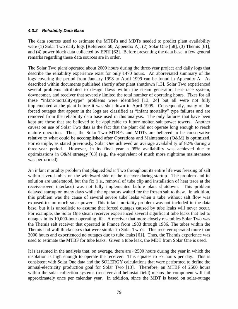
79

4.3.2 Reliability Data Base The data sources used to estimate the MTBFs and MDTs needed to predict plant availability were (1) Solar Two daily logs [Reference 60, Appendix A], (2) Solar One [58], (3) Themis [61], and (4) power block data collected by EPRI [62]. Before presenting the data base, a few general remarks regarding these data sources are in order. The Solar Two plant operated about 2000 hours during the three-year project and daily logs that describe the reliability experience exist for only 1470 hours. An abbreviated summary of the logs covering the period from January 1998 to April 1999 can be found in Appendix A. As described within documents published shortly after plant shutdown [13], Solar Two experienced several problems attributed to design flaws within the steam generator, heat-trace system, downcomer, and receiver that severely limited the total number of operating hours. Fixes for all these “infant-mortality-type” problems were identified [13, 24] but all were not fully implemented at the plant before it was shut down in April 1999. Consequently, many of the forced outages that appear in the logs are classified as “infant mortality” type failures and are removed from the reliability data base used in this analysis. The only failures that have been kept are those that are believed to be applicable to future molten-salt power towers. Another caveat on use of Solar Two data is the fact that the plant did not operate long enough to reach mature operation. Thus, the Solar Two MTBFs and MDTs are believed to be conservative relative to what could be accomplished after Operations and Maintenance (O&M) is optimized. For example, as stated previously, Solar One achieved an average availability of 82% during a three-year period. However, in its final year a 95% availability was achieved due to optimizations in O&M strategy [63] (e.g., the equivalent of much more nighttime maintenance was performed). An infant mortality problem that plagued Solar Two throughout its entire life was freezing of salt within several tubes on the windward side of the receiver during startup. The problem and its solution are understood, but the fix (i.e., removal of tube clip and installation of heat trace at the receiver/oven interface) was not fully implemented before plant shutdown. This problem delayed startup on many days while the operators waited for the frozen salt to thaw. In addition, this problem was the cause of several severe tube leaks when a tube without salt flow was exposed to too much solar power. This infant mortality problem was not included in the data base, but it is unrealistic to assume that forced outages caused by tube leaks will never occur. For example, the Solar One steam receiver experienced several significant tube leaks that led to outages in its 10,000-hour operating life. A receiver that more closely resembles Solar Two was the Themis salt receiver that operated in France from 1983 through 1986. The tubes within the Themis had wall thicknesses that were similar to Solar Two’s. This receiver operated more than 3000 hours and experienced no outages due to tube leaks [61]. Thus, the Themis experience was used to estimate the MTBF for tube leaks. Given a tube leak, the MDT from Solar One is used. It is assumed in the analysis that, on average, there are ~2500 hours during the year in which the insolation is high enough to operate the receiver. This equates to ~7 hours per day. This is consistent with Solar One data and the SOLERGY calculations that were performed to define the annual-electricity production goal for Solar Two [13]. Therefore, an MTBF of 2500 hours within the solar collection systems (receiver and heliostat field) means the component will fail approximately once per calendar year. In addition, since the MDT is based on solar-outage

80

hours, a value of 7 hours means that it could have taken up to 24 clock hours for the plant technicians to return the component to service (i.e., additional repair done at night). Since the plants analyzed in this report have near-base-load capacity factors of ~70%, it is not appropriate to use the steam power block reliability data from Solar One or Two, designed for a capacity factor of ~20%. EPRI has shown that fossil-fired power plants with high-capacity factors have a much longer MTBF than plants with low-capacity factors, attributed to less thermal cycling. Thus, reliability data for commercial steam plants with ~70% capacity factor were used in the analysis [61]29 and, for example, an MTBF for the steam generator and turbine system of 6130 hours (0.7*8760) means that these systems fail approximately once per calendar year. The EPRI reliability data are based on the analysis of subcritical steam-Rankine cycles. Since this analysis of next-generation power towers is also investigating supercritical steam-Rankine cycles, an attempt was made to obtain reliability data for supercritical plants. SNL’s technical librarian searched several data bases and could not find MTBF data for fossil-fired supercritical steam plants.30 Scheduled outages were deleted from the data bases and only data for unscheduled (or forced) outages are included. This was done because it is assumed the plant will be shut down for a total of one or two weeks per year to perform scheduled maintenance. This length of time is typical for commercial solar trough plants and appears to be more appropriate than the scheduled outage time at Solar One/Two. (Solar One and Two were first-of-a-kind plants and scheduled outages were conducted more often to check the status of the plant components.) Examples of scheduled maintenance activities include repainting of the receiver tubes and turbine overhaul. The MTBFs and MDTs derived from the four data sources are presented in Table 18. The columns are explained below: Component/subsystem – Each of these items can be found on the reliability block diagram shown in Figure 35. # of events – The number of times the component/subsystem led to a forced outage of the power plants shown in the Reference column. Fault Exposure Time (FET) (hrs) – The number of hours the component/subsystem was successfully operating at the power plant. If there were multiple similar components operating at the same time in the plant (e.g., pumps and valves), the value shown in the table is (FET)*(number of components).

29 EPRI studied seven combined cycle plants. Only data for the bottoming steam cycles were used. Typical steam

turbine size was ~100 MWe. 30 However, the availability/reliability of supercritical plants is expected to be high. According to Chandra Shekhar

(http://www.scribd.com/doc/3019711/Comparative-study-on-Subcritical-and-Super-Critical-Power-Cycles)“units installed in Japan over the past 10 years have achieved availabilities in the range of 98% to almost 100% with the exclusion of planned outages.” Also, according to Burns and McDonnell, “the availability of supercritical units built since 1990 is every bit as high as the subcritical units.” (www.massengineers.com/Documents/article-therankinecycle-013.pdf).

http://www.scribd.com/doc/3019711/Comparative-study-on-Subcritical-and-Super-Critical-Power-Cycles

81

Table 18. Reliability Data for Molten-Salt Plant Analysis.

Component or Subsystem

# of Events

Fault Exposure Time (hrs)

MTBF Nominal

(hrs)

MDT Nominal

(hrs)

Downtime Data (hrs)

Ref

Salt Flow Control Valves

3 19071 6357 8 1,8,15 Solar 2

Cold Salt Pumps 0 2934 Assume 2934

Assume 16

None Solar 2

Hot Salt Pumps 0 2934 Assume 2934

Assume 16

None Solar 2

Heat Trace System 2 1467 734 9 9(2) Solar 2 Rcvr Panel Drain Valves

1 17604 17604 3 3 Solar 2

Rcvr Inlet Tank Air System

5 1467 293 4 1,4(3),7 Solar 2

Rcvr Inlet Tank Level Instrument

1 1467 1467 3 3 Solar 2

Rcvr Tube Leak 0 3000 Assume 3000

14 0.7,3,6,13(2)16,22(4)

Solar 1 Themis

Rcvr Panel Replacement

Assume 15000

Assume 20

None

Rcvr Trips – Unknown Cause

6 1467 241 1.3 0.5(3),1.5, 2,3

Solar 2

Steam Gen Pumps 1 4401 4401 4 4 Solar 2 Steam Gen Tube Leak

Assume 61320

Assume 235

None

Steam Gen Trips – Unknown Cause

1 1467 1467 4 4 Solar 2

Plant Control Computers

8 1467 183 1.3 0.5,1(5),2, 2.5

Solar 2

Operator Error 2 1467 734 3 2,4 Solar 2 Heliostat Field Common Mode

2 1467 734 6.8 3.5,10 Solar 2

Heliostat Field Switchgear

1 5774 5774 7 7 Solar 1

Rankine Turbine 10 131470 13147 98 9.8(2),61(6), 300(2)

EPRI

Rankine Control System

11 131470 11952 5.8 4(2),6.4(2), 6(7)

EPRI

Rankine Circ Water Pumps

14 131470 9391 39 4,38(2), 43(11)

EPRI

Rankine Lube Oil System

2 131470 65736 125 125(2) EPRI

82

Table 18. Reliability Data for Molten-Salt Plant Analysis (continued).

Component or Subsystem

# of Events

Fault Exposure Time (hrs)

MTBF Nominal

(hrs)

MDT Nominal

(hrs)

Downtime Data (hrs)

Ref

Rankine Electric Generator

16 131470 8217 17 19(10), 14(6) EPRI

Rankine Condensate Pump

2 131470 65736 83 83(2) EPRI

Rankine Condenser 6 131470 21912 12 1.2,4.8(4),50 EPRI Service Water Sys 1 5774 5774 16 16 Solar 1 HVAC 3 1467 489 4.1 2,3.3,7 Solar 2 Maintenance Error 3 1467 489 6.2 2,6.5,10 Solar 2 Plant 4-kV Switchgear

1 5774 5774 0.4 0.4 Solar 1

Utility Grid 2 5774 2887 3.8 0.2,7.4 Solar 1 References – Solar Two [Appendix A], Solar One [58], Themis [61], EPRI [62]. MTBF Nominal (hrs) – The nominal value of MTBF is calculated as MTBF=FET/(# of events). If (# of events) is zero or assumed to be 1, a first-order MTBF based on engineering judgment is shown. MDT Nominal (hrs) – The nominal value of MDT is calculated as (Sum of downtime data)/(# of events). If no downtime data exist, a first-order MDT based on engineering judgment is shown. Downtime Data (hrs) – The downtime for each individual event is listed. The number of occurrences of the same downtime appears in parentheses. The downtimes listed are the number of hours solar energy collection was lost. For example, if the solar receiver failed one hour before sunset and it took 6 clock hours to repair the receiver, the downtime is 1 hour. However, because the steam-Rankine cycle is assumed to run 24/7 throughout much of the year, failures that occur after dark could cause the solar receiver to be shut down the next day due to a full hot tank.31 Thus, steam-Rankine downtimes are conservatively assumed to be based on clock hours. 4.3.3 Plant Availability Prediction Using the nominal MTBF and MDT values, Pro-Opta predicts a plant availability of 88.5% due to forced outages. Adding two weeks of scheduled outages would further reduce the overall annual availability to 85% = 88.5*(50/52). Pro-Opta can also be run to estimate the uncertainty associated with the availability prediction. Probability distributions are assigned to each MTBF and MDT and a sampling scheme is employed to propagate uncertainties through the logic model (fault tree or reliability block diagram). For cases with little failure data (like Solar Two) in which data are expressed as “X failures in Y hours of operation,” use of the gamma distribution is recommended by the guidance contained in the Pro-Opta User’s Manual. The “X” is the gamma-shape parameter and the “Y”

31 This occurred at Solar Two on a few occasions.

83

is the gamma-scale parameter. The mean of the gamma distribution is X/Y, which is convenient. However, the guidance warns the user that: “...it is important to realize that we are not trying to fit a gamma distribution to our data or implying that a gamma distribution is necessarily a good representation of the variability we might expect in failure rates. We recommend the gamma distribution in this situation because it reproduces the mean of our observations and gives us a reasonable representation of uncertainty. The gamma distribution is also easy to update if additional data become available.” To estimate the variability in MDT, the guidance in the Pro-Opta User’s Manual was followed:

• Given three or more downtime events, express the spread in downtimes as an empirical distribution. (For example, salt flow control valves [FCVs] in Table 18 have downtimes of 1, 8, and 15 hrs. A discrete-probability was created and each downtime was sampled with a 33.3% probability.)

• If just two downtimes are available, use a uniform distribution between high and low. (For example, see “Operator Errors” in Table 18).

• If a single downtime is all that is available, use the observed value as the best estimate in a triangular distribution and use judgment to add minimum and maximum values. (There are several cases like this in Table 18. The min/max values were assumed to be plus/minus a factor of 2.)

The result of the uncertainty analysis is shown in Figure 36. The mean plant availability due to forced outages is 88.3%, with a standard deviation of 1.8 points. 4.3.4 Plant Availability Improvement Opportunities The 85% nominal availability prediction is below the 90% goal established for initial commercial plants [3]. To achieve the goal requires an understanding of the most important contributors to the plant unavailability and an engineering evaluation of the most practical improvements. Pro-Opta was run to indentify the most important causes of plant unavailability. Table 19 displays the ranking according to system and Table 20 displays the ranking according to the basic failure event. As shown, the receiver system is expected to be the most important contributor to outages in a molten-salt plant. However, other systems and components are also predicted to be significant contributors.

84

Figure 36. Results from Pro-Opta uncertainty analysis of forced-outage availability.

Table 19. Contributors to Forced Outages Ranked by Systems Defined in Figure 35.

System Mean Fraction

1 Receiver 0.31252 Turbine Gen 0.14423 BOP/Other 0.13394 Steam Gen 0.11115 Heat Trace 0.10416 Plant Control 0.08587 Heliostat Field 0.07828 Transmission 0.01069 Hot Tank 0.0100

10 Cold Tank 0.009611 Cold Pump Trains <0.000512 Hot Pump Trains <0.0005

1.0000

85

Table 20. Contributors to Forced Outages Ranked by Basic Event.

Events Mean Fraction1 Rcvr Inlet Tank Air System 0.122802 Heat Trace System 0.104073 Maintenance Error 0.094704 Heliostat Field Common Mode Failures 0.067115 Rankine Turbine 0.060916 Control System Computers 0.054377 Rcvr Trips from Unknown Causes 0.046518 Steam Gen Tube Leak 0.034399 Rcvr Tube Leak 0.03244

10 Operator Error 0.0314211 Rankine Circ Water Pump 0.0306012 Service Water System 0.0238213 Steam Gen Trips from Unknown Causes 0.0235514 Rcvr Inlet Tank Level xmitter 0.0178515 Rankine Lube Oil System 0.0169416 Remote Heating Ventilation and Cooling 0.0153617 Rankine Electric Generator 0.0152618 Rcvr Panel Replacement 0.0121019 Rankine Condensate Pump 0.0115220 Heliostat Interface Switchgear 0.0111221 Hot Sump Flow Control Valve 0.0099822 Utility Grid 0.0099623 Rcvr Flow Control Valve 7 0.0099524 Rcvr Flow Control Valve 1 0.0098225 Rcvr Flow Control Valve 2 0.0098126 Rcvr Flow Control Valve 6 0.0097927 Rcvr Flow Control Valve 5 0.0097628 Rcvr Flow Control Valve 3 0.0097429 Steam Gen Salt Flow Control Valve 3 0.0096930 Steam Gen Salt Flow Control Valve 2 0.0096231 Steam Gen Salt Flow Control Valve 1 0.0096232 Rcvr Flow Control Valve 4 0.0096033 Cold Sump Flow Control Valve 0.0095634 Steam Gen Water Mix Pump 2 0.0083035 Steam Gen Water Mix Pump 3 0.0079836 Steam Gen Water Mix Pump 1 0.0079737 Rankine Condenser 0.0053738 Rankine Control System 0.0036639 Rcvr Panel Drain Valve 2 0.0016040 Rcvr Panel Drain Valve 5 0.0015741 Rcvr Panel Drain Valve 1 0.0015542 Rcvr Panel Drain Valve 6 0.0015543 Rcvr Panel Drain Valve 3 0.0015344 Rcvr Panel Drain Valve 7 0.0015345 Rcvr Panel Drain Valve 4 0.0015246 Rcvr Panel Drain Valve 8 0.0015047 4 kV Switchgear 0.0006348 Redundant Cold Salt Pumps <0.000549 Redundant Hot Salt Pumps <0.0005

1.00000

86

The ranking within these tables, as well as further review of the Solar Two MTBF and MDT data, can be used to identify reliability improvement opportunities to achieve the 90% availability goal. For example, lengthening the MTBF of the following events by a factor of 2 appears plausible and would likely have occurred naturally due to learning and optimization if Solar Two would have operated as long as Solar One.

• Receiver Inlet Tank Air System • Maintenance Error • Heat Trace System • Heliostat Field Common Mode Failures • Remote Station Heating Ventilation and Cooling • Control System Computers • Operator Error

It is also believed that more nighttime maintenance could reduce the average downtimes (MDTs) of the following items by 50%.

• Salt Flow Control Valves • Receiver Tube Leaks • Receiver Inlet Tank • Maintenance Errors • Heat Trace • Heliostat Field Common Mode Failures

In addition, more maintenance during nighttime and weather outages could reduce the needed annual scheduled outage time from two weeks to almost one week.32 Making all these changes to the data used in the analysis results in an annual availability of >90%. Pro-Opta was rerun to again determine the most important contributors to plant outages after the reliability improvements listed above are made. Table 21 gives the revised ranking.

32 Achieving one week scheduled outage per year may sound optimistic. However, the reduction in availability due

to the assumed one week of scheduled outages (51/52 = 0.98) can also be accomplished by scheduling nearly three weeks of outages in December and January since days are much shorter and weather is worse than an average week.

87

Table 21. Contributors to Forced Outages Assuming Reliability Improvements.

Events Mean Fraction

1 Rankine Turbine 0.082572 Rcvr Inlet Tank Air System 0.065233 Rcvr Trips from Unknown Causes 0.063994 Maintenance Error 0.060255 Heat Trace System 0.058346 Remote Heating Ventilation and Cooling 0.056097 Control System Computers 0.050648 Steam Gen Tube Leak 0.046699 Heliostat Field Common Mode Failures 0.0440210 Rankine Circ Water Pump 0.0422511 Service Water System 0.0331812 Steam Gen Trips from Unknown Causes 0.0325813 Rcvr Tube Leak 0.0325014 Operator Error 0.0292815 Rcvr Inlet Tank Level xmitter 0.0246116 Rankine Lube Oil System 0.0233517 Rankine Electric Generator 0.0211018 Rcvr Panel Replacement 0.0165919 Rankine Condensate Pump 0.0158920 Heliostat Interface Switchgear 0.0150621 Utility Grid 0.0137622 Steam Gen Water Mix Pump 2 0.0115323 Steam Gen Water Mix Pump 1 0.0109724 Steam Gen Water Mix Pump 3 0.0109725 Hot Sump Flow Control Valve 0.0091626 Rcvr Flow Control Valve 7 0.0090727 Rcvr Flow Control Valve 1 0.0090328 Rcvr Flow Control Valve 2 0.0090329 Rcvr Flow Control Valve 3 0.0090230 Rcvr Flow Control Valve 6 0.0090231 Steam Gen Salt Flow Control Valve 1 0.0090232 Rcvr Flow Control Valve 5 0.0090033 Steam Gen Salt Flow Control Valve 3 0.0089734 Steam Gen Salt Flow Control Valve 2 0.0089535 Rcvr Flow Control Valve 4 0.0089536 Cold Sump Flow Control Valve 0.0087937 Rankine Condenser 0.0074538 Rankine Control System 0.0050739 Rcvr Panel Drain Valve 2 0.0021940 Rcvr Panel Drain Valve 6 0.0021641 Rcvr Panel Drain Valve 5 0.0021642 Rcvr Panel Drain Valve 4 0.0021443 Rcvr Panel Drain Valve 3 0.0021444 Rcvr Panel Drain Valve 1 0.0021445 Rcvr Panel Drain Valve 7 0.0021346 Rcvr Panel Drain Valve 8 0.0020947 4 kV Switchgear 0.0008748 Redundant Cold Salt Pumps <0.000549 Redundant Hot Salt Pumps <0.0005

1.00000

88

89

Chapter 5 Levelized-Energy Cost Calculations

In this chapter the data presented in the previous chapters regarding performance and reliability are brought together with costs from the DOE Power Tower Roadmap to calculate an LCOE. The LCOE is the levelized 30-year price that would have to be charged for the electricity by an IPP given the financing parameters required by the debt and equity investors as defined in the project proforma. The financing parameters selected for this analysis were those used within the DOE Power Tower Roadmap [3]. They are summarized in Table 22. The LCOE for the central receiver plants were calculated with the following simple equation: LCOE = FCR*Installed Capital Costs + Annual O&M Costs (17) Annual Energy * Plant Availability

Table 22. IPP Financing Parameters.

General Analysis Period 30 yrs Inflation Rate 2.5%

Taxes and Insurance Federal Tax 35%/yr State Tax 8%/yr Property Tax 0.5%/yr Sales Tax 7.75%/yr Insurance 0.5%/yr Salvage Value 0 Construction Period Overnight

IPP Financing Parameters Loan term 20 yrs Loan rate 8%/yr Debt/equity fraction 54/46 (optimized) Equity required IRR 14% Minimum debt coverage ratio 1.4 Cashflows all positive? Yes PPA escalation rate 1.2%/yr

Tax Incentives (Equity Measures33) Investment tax credit (ITC) 10% Accelerated depreciation 5-yr MACRS

The fixed charge rate (FCR) is a single parameter that represents all the capital-financing-related assumptions in the analysis. The value used in the analysis was 7.5% based on the financial 33 Detailed studies performed by the California Energy Commission [64, 65] have shown that a combination of the

permanent federal ITC of 10%, 5-year or shorter accelerated depreciation, and property tax reductions, approximately equalizes the tax burden paid by solar power plants and fossil-fired plants of similar size. Thus, the “tax incentives” are actually “tax equity measures.”

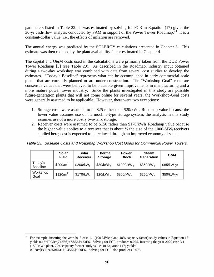
90

parameters listed in Table 22. It was estimated by solving for FCR in Equation (17) given the 30-yr cash-flow analysis conducted by SAM in support of the Power Tower Roadmap.34 It is a constant-dollar value, i.e., the effects of inflation are removed. The annual energy was predicted by the SOLERGY calculations presented in Chapter 3. This estimate was then reduced by the plant availability factor estimated in Chapter 4. The capital and O&M costs used in the calculations were primarily taken from the DOE Power Tower Roadmap [3] (see Table 23). As described in the Roadmap, industry input obtained during a two-day workshop was combined with data from several cost studies to develop the estimates. “Today’s Baseline” represents what can be accomplished in early commercial-scale plants that are currently planned or are under construction. The “Workshop Goal” costs are consensus values that were believed to be plausible given improvements in manufacturing and a more mature power tower industry. Since the plants investigated in this study are possible future-generation plants that will not come online for several years, the Workshop-Goal costs were generally assumed to be applicable. However, there were two exceptions:

1. Storage costs were assumed to be $25 rather than $20/kWht Roadmap value because the lower value assumes use of thermocline-type storage system; the analysis in this study assumes use of a more costly two-tank storage.

2. Receiver costs were assumed to be $150 rather than $170/kWht Roadmap value because the higher value applies to a receiver that is about ½ the size of the 1000-MWt receivers studied here; cost is expected to be reduced through an improved economy of scale.

Table 23. Baseline Costs and Roadmap Workshop Cost Goals for Commercial Power Towers.

Solar Field

Solar Receiver

Thermal Storage

Power Block

Steam Generation O&M

Today’s Baseline $200/m2 $200/kWt $30/kWht $1000/kWe $350/kWe $65/kW-yr

Workshop Goal $120/m2 $170/kWt

$20/kWht $800/kWe $250/kWe $50/kW-yr

34 For example, inserting the year 2013 case 1.1 (100 MWe plant, 48% capacity factor) study values in Equation 17

yields 0.15=[FCR*(743E6)+7.8E6]/423E6. Solving for FCR produces 0.075. Inserting the year 2020 case 3.1 (150 MWe plant, 72% capacity factor) study values in Equation (17) yields: 0.078=[FCR*(850E6)+10.35E6]/950E6. Solving for FCR also produces 0.075.

91

The Roadmap capital costs only represent direct costs. To convert to “Installed Costs” several indirect-type costs must be added. Indirects include Engineering, Procurement, and Construction costs, as well as other items such as project development costs and sales tax. Historical studies have shown that Indirects can be 40% or more of the direct costs, especially for early commercial power plants. However, as the technology matures and after several similar plants are deployed, the indirect-cost multiplier can be substantially reduced. In this study, this factor is assumed to be 1.25. Results of LCOE Calculations A summary of the LCOE calculations for all six case studies is presented in Table 24. The example below shows how Equation (17) was used to calculate the LCOE for the case entitled “subcritical wet.” Installed Capital Costs = (Direct Capital Costs) * Indirect Cost Multiplier = ($693E6) * 1.25 = $867E6 Annual O&M Costs = Fixed O&M Cost + Variable O&M Cost Fixed O&M Cost = $50/kWe-yr * 145000 kWe = $7.3E6/yr Variable O&M Cost = $3/MWhe * 775000 MWhe/yr = $2.3E6/yr Annual O&M Cost = $9.6E6/yr Plant Availability = 90% appears to be feasible from reliability analysis in Chapter 4 Annual Energy = 861E6 kWh from SOLERGY analysis in Chapter 3 LCOE = 0.075*$867E6 + $9.6E6 = 0.096 $/kWhe 861E6 kWh * 0.9

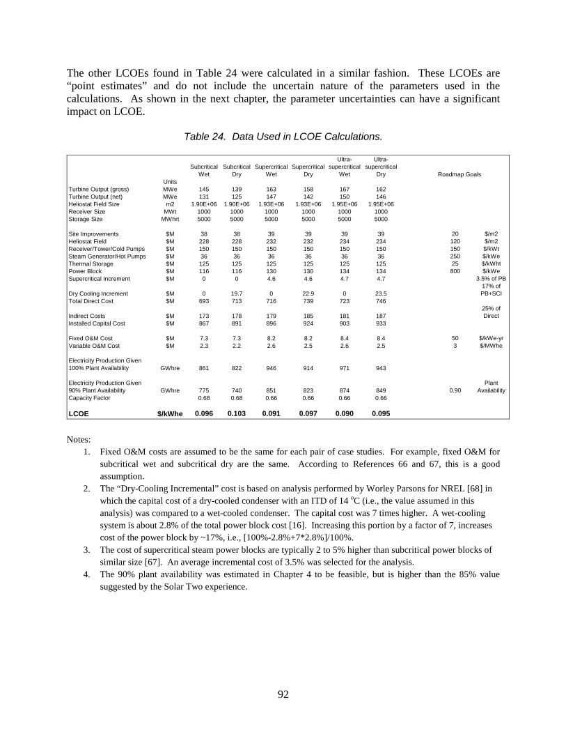
92

The other LCOEs found in Table 24 were calculated in a similar fashion. These LCOEs are “point estimates” and do not include the uncertain nature of the parameters used in the calculations. As shown in the next chapter, the parameter uncertainties can have a significant impact on LCOE.

Table 24. Data Used in LCOE Calculations.

Subcritical Wet

Subcritical Dry

Supercritical Wet

Supercritical Dry

Ultra-supercritical

Wet

Ultra-supercritical

Dry Roadmap GoalsUnits

Turbine Output (gross) MWe 145 139 163 158 167 162Turbine Output (net) MWe 131 125 147 142 150 146Heliostat Field Size m2 1.90E+06 1.90E+06 1.93E+06 1.93E+06 1.95E+06 1.95E+06Receiver Size MWt 1000 1000 1000 1000 1000 1000Storage Size MWhrt 5000 5000 5000 5000 5000 5000

Site Improvements $M 38 38 39 39 39 39 20 $/m2Heliostat Field $M 228 228 232 232 234 234 120 $/m2Receiver/Tower/Cold Pumps $M 150 150 150 150 150 150 150 $/kWtSteam Generator/Hot Pumps $M 36 36 36 36 36 36 250 $/kWeThermal Storage $M 125 125 125 125 125 125 25 $/kWhtPower Block $M 116 116 130 130 134 134 800 $/kWeSupercritical Increment $M 0 0 4.6 4.6 4.7 4.7 3.5% of PB

Dry Cooling Increment $M 0 19.7 0 22.9 0 23.517% of PB+SCI

Total Direct Cost $M 693 713 716 739 723 746

Indirect Costs $M 173 178 179 185 181 18725% of Direct

Installed Capital Cost $M 867 891 896 924 903 933

Fixed O&M Cost $M 7.3 7.3 8.2 8.2 8.4 8.4 50 $/kWe-yrVariable O&M Cost $M 2.3 2.2 2.6 2.5 2.6 2.5 3 $/MWhe

Electricity Production Given 100% Plant Availability GWhre 861 822 946 914 971 943

Electricity Production Given 90% Plant Availability GWhre 775 740 851 823 874 849 0.90

Plant Availability

Capacity Factor 0.68 0.68 0.66 0.66 0.66 0.66

LCOE $/kWhe 0.096 0.103 0.091 0.097 0.090 0.095 Notes:

1. Fixed O&M costs are assumed to be the same for each pair of case studies. For example, fixed O&M for subcritical wet and subcritical dry are the same. According to References 66 and 67, this is a good assumption.

2. The “Dry-Cooling Incremental” cost is based on analysis performed by Worley Parsons for NREL [68] in which the capital cost of a dry-cooled condenser with an ITD of 14 oC (i.e., the value assumed in this analysis) was compared to a wet-cooled condenser. The capital cost was 7 times higher. A wet-cooling system is about 2.8% of the total power block cost [16]. Increasing this portion by a factor of 7, increases cost of the power block by ~17%, i.e., [100%-2.8%+7*2.8%]/100%.

3. The cost of supercritical steam power blocks are typically 2 to 5% higher than subcritical power blocks of similar size [67]. An average incremental cost of 3.5% was selected for the analysis.

4. The 90% plant availability was estimated in Chapter 4 to be feasible, but is higher than the 85% value suggested by the Solar Two experience.

93

Chapter 6 Uncertainty Analysis

The parameters employed in the analysis of plant performance, cost, and reliability are not known precisely. In this chapter, uncertainty ranges are estimated for the parameters associated with the subcritical plant with dry cooling, followed by a determination of each parameters effect on the overall uncertainty in LCOE. As will be shown, this type of analysis is useful to planning and prioritizing future central receiver research. 6.1 Goal and Philosophy R&D programs for central receiver technology are conducted to reduce uncertainty regarding performance, cost, etc., so that more credible predictions of economic viability can be made. The systems analysis presented in this report attempts to integrate all the major parameters that have an influence on economic predictions. Therefore, if it can be determined that the parameters are most important to the uncertainty in the predictions of LCOE, this information can be used to help identify and prioritize future central receiver research. This is the goal of the work presented in this chapter. Uncertainty ranges were placed on the basic analysis parameters and these ranges were combined through the analytical models and a constrained sampling technique to obtain an uncertainty range on LCOE. This uncertainty was then decomposed, using linear regression techniques, to determine the influence of the individual analysis parameters. Financial parameters, such as FCR, can have a large impact on LCOE. However, uncertainty limits were not placed on them because they are not engineering-related and even if they were identified to be important to uncertainty, they could not be addressed by an R&D program. Based on the above discussion, it is evident the uncertainty analysis does not represent a rigorous statistical treatment. However, it represents the current state of knowledge regarding the uncertainties associated with the technology and the method appears useful to help plan and prioritize future R&D activities. 6.2 Methodology The analysis methodology steps are shown in Figure 37 and explained below.

Figure 37. Methodology used in uncertainty analysis.

94

Screening Analysis A screening analysis was conducted first. The goal was to reduce the several hundred parameters in the study to a smaller number more tractable for analysis. The number was reduced by (1) grouping the parameters, (2) treating parameters that are highly certain as point values or equations with no uncertainty, and (3) ignoring uncertainties associated with parameters that have been shown by other studies to have a small effect on LCOE. An example of parameter grouping is heliostat costs. Rather than subdividing heliostat costs into mirror costs, drive costs, motor costs, etc., these parameters were treated as a single parameter. An example of a set of parameters treated as an equation with no uncertainty is gross steam-Rankine-cycle efficiency. For a given plant design, known heat inputs, and ambient conditions, professional computer software used to predict steam-plant efficiency (such as the GateCycle code used here) have been validated with data collected at many different steam plants over the years. Reliability parameters were screened using the Pro-Opta importance ranking presented in Table 20. Based on that ranking, it was decided to input the plausible ranges for the reliability parameters associated with the top 20 components and to ignore the rest. 35 Since each component is characterized by a MTBF and MDT, 40 reliability parameters are included. Experience gained during the modeling of Solar Two was used to screen the uncertain annual performance parameters used by SOLERGY. The nine parameters listed in Table 25 were selected. Uncertainty limits were placed on all capital cost and O&M parameters. Limits were even placed on low-cost items that would not have a significant impact on the results. This was done to test the predictive capability of the computer code employed in the analysis. The nine cost parameters listed in Table 26 were selected. The screening analysis identified 58 parameters for further study: 40 reliability, 9 annual performance, and 9 cost. Establishing Plausible Ranges for Parameters The 58 parameters and associated ranges are summarized in Tables 25, 26, and a subset of Table 18. The values presented in previous chapters for performance, cost, and reliability were taken to be “best-estimate” values within a plausible range of values. Plausible ranges on the parameters were established through use of experimental evidence and expert judgment. The plausible range is expressed by a probability distribution. In general, the distributions assigned to each parameter followed the guidance given in the Pro-Opta user’s guide [17]. For example, when actual X/Y data were available (i.e., X results in Y tests), gamma and discrete-probability

35 The Pro-Opta uncertainty analysis described in Chapter 4 included plausible ranges for all the reliability

parameters.

95

distributions (DPDs) were used. However, if little or no data are available, experience is used to estimate lower and upper bounds for the parameters. If only the bounds can be estimated, a uniform probability distribution is assumed. If a most likely value is known to exist within the bounds, a triangular distribution is used. Also stated in the tables are the rationales used to establish the ranges. The information presented is sufficient to understand the rationales; if more detail is needed, the reader should refer to the discussion of these parameters in Chapters 3 and 4.

Table 25. Uncertainty Distributions for SOLERGY Parameters.

Parameter Best Estimate Distribution Rationale

Receiver Absorptance 0.94 Triangular 0.91-0.95

Upper bound was measured at Solar One during its final three years [51]. Lower bound is plausible because salt receiver has higher flux level and salt leaks can cause Pyromark coating to degrade.

Heliostat Cleanliness 0.95 Triangular 0.93-0.97

Best estimate is typical value at Kramer Junction trough plants [50]. Upper bound may be achievable with more frequent washes. Lower bound assumed symmetric to upper bound.

Receiver Turn Down 16% Triangular 10%-16%

Best estimate based on data from Solar Two [13]. It is feasible that a more aggressive operating procedure and/or design could reduce the turndown ratio.

Heliostat Availability 0.99 Triangular 0.970-0.995

Best estimate based on Solar One data [51]. Upper and lower bounds are plausible depending on the design of the heliostat and the field control system.

Receiver Thermal Losses 30 kWt/m2

Triangular 20 to 30kWt/m2

Best estimate based on Solar Two data [15]. The radiation and convection model in SAM predicts lower thermal losses for Solar Two. The difference between model and data is unresolved.

Parasitic Multiplier 1 Uniform ±20%

Since the SOLERGY and GateCycle parasitic power models were based on generic information, it was judged they could be in error by +/- 20%.

Unusable DNI 0% Triangular 0% to 40%

Solar Two demonstrated that the receiver can operate through very rapid insolation transients. Thus, the best estimate is that plant operators do not defocus field during cloudy weather. However, to reduce thermal fatigue the operators may decide to defocus in some cloud situations; 40% implies that operators will shut down if average DNI is less than 40% of clear-sky value within a 15-minute period.

Heliostat Stow Wind Speed 40 mph

Triangular 25 to 40 mph

Best estimate is from Solar One operations experience [51]. However, industry is currently considering designs that may stow as low as 25 mph.

Wind Effect on Beam Spillage

Not significant

Uniform 0 to 1.5%

Best estimate assumes very rigid heliostats. If heliostats are designed to meet minimum wind specs in Design Basis Document [11] up to ~1.5% annual loss could occur for Barstow-type weather based on DELSOL/SOLERGY sensitivity study.

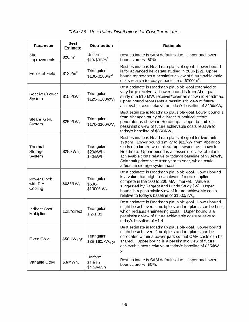
96

Table 26. Uncertainty Distributions for Cost Parameters.

Parameter Best Estimate Distribution Rationale

Site Improvements $20/m2

Uniform $10-$30/m2

Best estimate is SAM default value. Upper and lower bounds are +/- 50%.

Heliostat Field $120/m2 Triangular $100-$180/m2

Best estimate is Roadmap plausible goal. Lower bound is for advanced heliostats studied in 2006 [22]. Upper bound represents a pessimistic view of future achievable costs relative to today’s baseline of $200/m2.

Receiver/Tower System $150/kWt

Triangular $125-$180/kWt

Best estimate is Roadmap plausible goal extended to very large receivers. Lower bound is from Abengoa study of a 910 MWt receiver/tower as shown in Roadmap. Upper bound represents a pessimistic view of future achievable costs relative to today’s baseline of $200/kWt.

Steam Gen. System $250/kWe

Triangular $170-$300/kWe

Best estimate is Roadmap plausible goal. Lower bound is from Abengoa study of a larger subcritical steam generator as shown in Roadmap. Upper bound is a pessimistic view of future achievable costs relative to today’s baseline of $350/kWe.

Thermal Storage System

$25/kWht Triangular $20/kWht-$40/kWht

Best estimate is Roadmap plausible goal for two-tank system. Lower bound similar to $22/kWt from Abengoa study of a larger two-tank storage system as shown in Roadmap. Upper bound is a pessimistic view of future achievable costs relative to today’s baseline of $30/kWht. Solar salt prices vary from year to year, which could affect the storage system cost.

Power Block with Dry Cooling

$835/kWe Triangular $600-$1000/kWe

Best estimate is Roadmap plausible goal. Lower bound is a value that might be achieved if more suppliers compete in the 100 to 200 MWe market. Value is suggested by Sargent and Lundy Study [69]. Upper bound is a pessimistic view of future achievable costs relative to today’s baseline of $1000/kWe.

Indirect Cost Multiplier 1.25*direct

Triangular 1.2-1.35

Best estimate is Roadmap plausible goal. Lower bound might be achieved if multiple standard plants can be built, which reduces engineering costs. Upper bound is a pessimistic view of future achievable costs relative to today’s baseline of ~1.4.

Fixed O&M $50/kWe-yr Triangular $35-$60/kWe-yr

Best estimate is Roadmap plausible goal. Lower bound might be achieved if multiple standard plants can be collocated within a power park so that O&M costs can be shared. Upper bound is a pessimistic view of future achievable costs relative to today’s baseline of $65/kW-yr.

Variable O&M $3/MWhe Uniform $1.5 to $4.5/MWh

Best estimate is SAM default value. Upper and lower bounds are +/- 50%.

97

Performing LCOE Uncertainty Analysis The LCOE for the plant can be expressed by the following equation: LCOE = FCR * IND* (DC1 + DC2 + ... DC9) + O&MF + O&MV*AE*AVAIL (18) AE(P1, P2, ... P9) * AVAIL(R1, R2, ... R40) where FCR = fixed charge rate = 0.075, IND = Indirect cost multiplier, DCx = Direct costs associated with system X, O&MF = Fixed O&M costs, O&MV = Variable O&M costs, AE = SOLERGY prediction of annual energy given variations in performance parameters P1 through P9, and AVAIL = Pro-Opta prediction of plant availability given variations in reliability parameters R1 through R40. To obtain uncertainty limits on LCOE, the probability distributions associated with each of the 58 parameters must be convolved via the above function. This was done through use of Latin-Hypercube sampling (LHS) [21]. Unlike the Monte Carlo approach, which employs random sampling, LHS uses a constrained sampling scheme. LHS requires a fewer number of computer runs than Monte Carlo and can yield more precise estimates. The LHS computer code was used to sample the ranges of the 58 parameters. This sampling produced 301 different combinations of parameter values. Equation (18) was then solved for each combination to produce 301 values of LCOE.36 The LCOE values were then grouped to produce a cumulative distribution function (CDF), as shown in Figure 38. The analysis was performed two times assuming two different sets of reliability parameters, as explained in Section 6.3.

36 SOLERGY was run 301 times. Siri Khalsa developed a routine for another project to automate this process [70].

98

0

0.1

0.2

0.3

0.4

0.5

0.6

0.7

0.8

0.9

1

0.08 0.09 0.1 0.11 0.12 0.13 0.14

LCOE ($/kWh)

Cum

ulat

ive

Prob

abili

tyCDF - 90% Availability

CDF - 85% Availability

Figure 38. LCOE CDFs for the subcritical plant with dry cooling.

Identifying Parameters Important to Uncertainty in LCOE The Statisica computer code was used to identify and rank the parameters that are important to LCOE uncertainty [20] (called “stepwise rank regression”). The code attempts to fit a linear regression model to data sets of dependent versus independent variables and contains algorithms that protect against overfit of the data. In the case analyzed here, each of the 301 solutions to Equation (18) constituted a data set. The model is of the form: j

jj XBBY *0 ∑+= (19)

where Y = dependent variable (LCOE), B0 = intercept, Bj = regression coefficients, and Xj = independent variables (the 58 parameters).

99

The independent variables that are most important to the predictive capability of the regression model are brought into the model first, followed by variables of less importance. An R2 statistical test is performed to determine the goodness of fit. The R2 value varies between zero and one and should be close to one if the model predicts the observed values adequately. In addition to the intercept and regression coefficients, the code also calculates standardized regression coefficients (SRCs) for each independent variable. The SRCs are used to rank the independent variables in terms of their effect on uncertainty, and have the following physical interpretation: if all independent variables are increased or decreased by the same fraction of their standard deviation, the SRC is a relative ranking of how the dependent variable changes. The SRCs are presented in Figure 39. The linear regression models identified by Statistica are very good since the R2 values (~0.95) are close to unity for both analyses. SRC values have positive and negative signs. If the SRC has a positive value, an increase in the value of the independent variable will cause an increase in the dependent variable. If SRC is negative, an increase in the independent variable will cause a decrease in the dependent. Examples are: since collector cost is positive, an increase in this parameter will cause an increase in LCOE; since heliostat cleanliness is negative, an increase in this parameter will cause a decrease in LCOE. Please note that the inverse of MTBF (also called “failure rate”) is plotted.

100

Figure 39. Top 20 contributors to LCOE uncertainty

given 85% (top) and 90% (bottom) plant availability parameters.

101

6.3 Results Two separate analyses were run to represent the two different plant-availability studies described in Chapter 4: an 85% availability case study and a 90% case study. According to Figure 38, the LCOE for the subcritical plant with dry cooling is between 9 and 12.5 cents/kWh, given a nominal plant availability of ~90%. This range is applicable if reliability improvements relative to the Solar Two experience can be achieved. These improvements were described in Chapter 4 and are summarized in Table 27. It is interesting to compare this CDF with the 10.3-cent/kWh point estimate calculated for this case study in Chapter 5 (see Table 24). According to the CDF, the probability of achieving 10.3 cents or less is only ~20%; the more likely median value is shown to be ~10.8 cents. This occurred because several of the uncertainty distributions were not symmetric about the nominal value. For example, heliostat costs were characterized by a triangular distribution with upper and lower bounds of $100 and $180/m2, but with a most likely value of $120/m2. This comparison clearly shows that it is important to include uncertainties when estimating LCOE. For the 85% plant availability case, the MTBF and MDT uncertainty distributions based on the Solar Two reliability experience were used (see Table 18). Combining these reliability distributions with the performance and cost distributions described in Tables 25 and 26, respectively, yielded the ranking shown at the top of Figure 39. This figure indicates that heliostat cost (1) has the most important influence on LCOE uncertainty with the following parameters having approximately one-half to one-sixth the influence: storage cost (2), indirect cost (3), site development cost (4), receiver/tower cost (5), power block cost (6), fixed O&M cost (7), parasitic consumption (8), heat trace MTBF (9), and power block MDT (10). Other parameters in the analysis were ranked below these ten. Since heliostats comprise more than 1/3 of the total plant cost and have a large uncertainty in future cost, it is not surprising they dominate. Other studies have concluded the same [1, 71]. For the 90% plant availability case, the MTBF and MDT uncertainty distributions described in Table 27 were used. Combining these reliability distributions with the same performance and cost distributions yielded the ranking shown at the bottom of Figure 39. Comparison of the top versus bottom shows the top eight parameters to be the same. However, the ranking below that is different. Noticeably absent are the following reliability parameters that were assumed to be improved in the 90% plant availability case study: heat-trace MTBF, receiver inlet tank MDT and MTBF, maintenance error and operator error MTBFs, and heliostat field common-mode failure MTBF. Since the influences of these parameters are now much less, other uncertain parameters such as “wind-effect on heliostat spillage” and “receiver absorptance” have moved up the top-20 list. Since the purpose of central receiver R&D is to reduce the uncertainty associated with predictions of the economic viability of the technology, this importance ranking should help prioritize future central receiver research. The analysis indicates that primary emphasis should be placed on narrowing the uncertainty limits associated with several capital cost categories, especially heliostats.

102

Table 27. Changes to Uncertainty Distributions for Improved Plant Availability Study.

Parameter Best

Estimate (hrs)

Distribution Rationale

Receiver Inlet Tank MTBF 586 Triangular

293 to 586 Lengthening MTBF by a factor of 2 appears plausible through learning. Worst-case bound is Solar Two experience.

Maintenance Error MTBF 978 Triangular

489 to 978 Heat Trace System MTBF 1468 Triangular

734 to 1468 Heliostat Field Common Mode Failure MTBF 1468 Triangular

734 to 1468 Remote Station HVAC MTBF 978 Triangular

489 to 978 Control System Computers MTBF 366 Triangular

183 to 366

Operator Error MTBF 1468 Triangular 734 to 1468

Receiver Tube Leak MDT 7 Triangular

7 to 14 Reducing MDT by a factor of 2 appears plausible through learning. Worst-case bound is Solar Two experience.

Salt Flow Control Valve MDT 4 Triangular

4 to 8

Receiver Inlet Tank MDT 2 Triangular

to 4

Maintenance Error MDT 3.1 Triangular 3.1 to 6.2

Heat Trace MDT 4.5 Triangular 4.5 to 9

Heliostat Field Common Mode Failure MDT 3.4 Triangular

3.4 to 6.8

Scheduled Outages 1 week None

Reducing scheduled outage from 2 to 1 weeks/yr could happen with more nighttime scheduled maintenance.

103

Chapter 7 Conclusions

Since completion of the Solar Two molten-salt power tower demonstration in 1999, the solar industry has been developing initial commercial-scale projects that are 3 to 14 times larger. The first commercial plant, Gemasolar, began operating in Spain in 2011 and the first commercial U.S. plant is now under construction near Tonopah, Nevada. Like Solar Two, these initial plants will power subcritical steam-Rankine cycles using molten salt with a temperature of 565 °C. Several of these plants are expected to be built over the next decade. The main question explored in this study is whether there is significant economic benefit to develop future molten-salt plants that operate at a higher receiver outlet temperature. Higher temperatures would allow the use of supercritical steam cycles that achieve an improved efficiency relative to today’s subcritical cycle (~50% versus ~42%). The 2010 DOE/Industry Roadmap also suggested that future molten salts could benefit from higher operating temperatures. Thus, the LCOE of a 565 °C subcritical baseline plant was compared with possible future-generation plants that operate at 600 or 650 °C. The receiver thermal ratings of the plants that were studied are the maximum practical size originally identified by the DOE program in the late 1980s (~1000 MWt). This is 1.7X scaleup of the Tonopah plant. In addition, like Gemasolar, all plants incorporate 15 hours of thermal storage to achieve high solar-only capacity factors.37 The seven major conclusions of the study are underlined and discussed below. Significant economic benefit is realized by increasing salt temperature from 565 to 600 °C. There is no compelling argument to increase salt temperature to 650 °C. The analysis showed that increasing salt temperature from 565 to 650 oC should reduce LCOE by ~8%. However, ~80% of that reduction can be achieved by raising the temperature to only 600 °C. LCOE is direct function of power block efficiency. As shown in the analysis, raising salt temperature to 600 °C increases the design-point efficiency from 43% to 48.4% and raising it to 650 °C results in 49.6% (wet cooling cases). Thus, ~80% of the efficiency improvement is achieved by increasing the temperature to 600 °C. Figure 40 is helpful in understanding this nonlinear behavior of temperature versus efficiency. Figure 40 compares the steam cycles powered by the three salt temperatures on a temperature-entropy (TS) diagram. The efficiency of a particular steam cycle is the ratio of the area enclosed by the cycle (Aencl) divided by the total area (defined as Aencl plus the area of the rectangle below Aencl extrapolated to absolute zero). It can be seen that a significant increase in Aencl occurs when switching from a subcritical to a supercritical cycle because the thermodynamic cycle “jumps over the steam dome.” However, after jumping over the dome, only a small incremental increase in Aencl occurs when increasing temperatures from supercritical to ultra-supercritical.

37 DOE is currently directing a large R&D program to develop baseload solar technology that is a direct

replacement of coal-fired power plants. Coal produces 50% of the power in the United States.

104

Figure 40. Comparison of steam-Rankine thermodynamic cycles. The subcritical cycle is powered by 565 oC salt. The supercritical and ultra-supercritical cycles are powered by 600 and 650 oC salt, respectively. To improve clarity, only the

extremes (i.e., dots) of the ultra-supercritical cycle are shown; the full-cycle shape is similar to the supercritical cycle.

Limiting salt temperatures to 600 oC avoids several technical issues that would need to be addressed if it was desired to operate at 650 °C. For example, salt corrosion of receiver materials is fairly well understood at 600 oC, but not at 650 °C. Operation at 650 °C would likely require the development of a new solar salt, new receiver materials, and/or the inclusion of an oxygen-blanking system to reduce the rate of corrosion. This could increase costs beyond the estimates provided in this report, which could easily eliminate the remaining possible reduction in LCOE. To achieve the LCOE reduction possible with supercritical power towers will likely require a scale-up of today’s solar technology and a scale-down of today’s steam-power blocks. All the subcritical and supercritical plants investigated in this study are comprised of a 1000-MWt receiver, 15 hours of storage (5000 MWht), and a steam power block with a nominal rating between 140 and 165 MWe. Not all the technologies needed to build these plants currently exist. For example, the world’s largest molten-salt power tower now under construction in Nevada consists of a 585-MWt receiver and a 2900-MWht thermal storage system. Thus, the receiver/storage technologies studied here are 1.7X larger than today’s technology. Subcritical

105

steam-power blocks with an output of ~150 MWe currently exist. However, the smallest supercritical power blocks available today are ~450 MWe. Thus, the supercritical power blocks studied here are about 1/3 the size of today’s technology. An important assumption was made that it is not practical to thermally cycle a supercritical-power block on a daily basis; it will need to operate nearly 24/7, much like it does in a coal plant. The much higher steam pressures (≥300 bar supercritical versus 125 bar subcritical) will result in very thick pipe walls and turbine casings, which should greatly increase startup time relative to a subcritical plant. The 1000-MWt receiver size was selected as a “happy medium” to meet the technological and economic constraints that could likely be required to deploy a successful supercritical power tower. That is, the 1000-MWt size has been predicted in previous studies to result in a lower LCOE due to an improved economy of scale relative to ~500-MWt receivers. Also, preliminary discussions with supercritical power block providers suggest that scaling down by a factor of 3 may be feasible. Combining these two statements with the expected need to run baseload results in the 1000 MWt/5000 MWh/~150 MWe combination recommended here. A salt receiver with a flux limit that is 25% higher than demonstrated at Solar Two can likely be built to achieve a 30-year lifetime. The peak flux at Solar Two was 800 suns. The receivers investigated in this study increased the peak flux to 1000 suns. A higher flux receiver is desirable because less heat-exchange area is needed to absorb a given amount of power. A reduction in area reduces heat loss (improves efficiency) as well as the cost of the receiver. The recommended receiver tube materials are different than the 316SS used at Solar Two. Depending on the receiver outlet temperature, the following materials were investigated and appear to be possible: (1) 565 °C – Incoloy 800, Inconel 625-LCF, and Haynes 230, (2) 600 °C – Incoloy 800 and Haynes 230, and (3) 650 °C – perhaps Haynes 230. Further analysis and experiments are recommended, but the analysis conducted here suggests that these tube materials are appropriate and meet the 30-year lifetime requirements dictated by low-cycle thermal fatigue, salt corrosion, and strength as specified in the ASME boiler and pressure vessel code. Reliability improvements relative to the experience at Solar Two need to occur to achieve the 90% plant availability goal. Several problems and design flaws identified during startup and commissioning led to significant downtime at Solar Two. Consequently, the plant operated for less than 2000 total hours during the project lifetime. This short time precluded the achievement of a mature operating mode. Thus, even after correcting for known infant-mortality problems, an analysis of the existing data suggests ~85% plant availability, which is short of the 90% goal for the technology. Several of the remaining reliability problems would likely have been resolved through the natural course of learning if the plant would have run longer, but that is conjecture. (For example, Solar One operated for 10,000 hours and plant availability steadily improved from an initial value of 82% to 95%.) Several plant systems and components were targeted for improvement to achieve the 90% goal.

106

The LCOE of dry-cooled power tower is ~0.6 cents/kWh higher than a wet-cooled power tower. Critics of solar power towers often state the technology is not sustainable because they consume a large amount of water and are installed in desert regions that do not have this resource. Dry cooling of the condenser can reduce water consumption by more than 90%. A detailed comparison of wet versus dry cooling in this study suggests that LCOE will increase by ~0.6 cents/kWh if dry cooling is used. The incremental capital cost to implement dry cooling is insignificant relative to the total cost of the plant. However, LCOE is increased because annual efficiency is degraded from 16.7% to 16.0% for the subcritical plant using 565 oC salt and from 18.1% to 17.5% for the supercritical plant using 600 oC salt. The LCOE of future molten-salt power towers is uncertain and that uncertainty is dominated by the predicted cost for heliostats. Heliostats now being deployed within initial commercial projects cost about $200 to $250/m2. Significant cost reductions are predicted as the power-tower industry matures due to increases in manufacturing volume and technology improvements. But there is a large variation in expected future costs. An analysis of the causes of LCOE uncertainty found that heliostats had the dominant influence, followed by several other capital cost categories. Since heliostats comprise more than 1/3 of the total plant cost and have a large uncertainty in future cost, it is not surprising they dominate. Uncertainties in several performance and reliability parameters were also found to have a significant influence on LCOE uncertainty. Since the purpose of R&D is to reduce the uncertainty associated with predictions of the economic viability of the technology, the developed importance ranking can help prioritize future central receiver research. The Pro-Opta reliability software tool was validated with power tower data and is a useful power-tower analysis tool. Most of the software tools used in this study (DELSOL, SOLERGY, SAM, GateCycle, and Statistica) have been used within previous studies of power towers. However, this is the first study to use Pro-Opta software to analyze power tower reliability issues. To ensure its validity, software predictions were compared with reliability data collected during the Solar One project. The prediction of plant availability was very close to the data. Pro-Opta has also been used to study wind-farm power plants. This SNL-developed tool is easy to use and is available for free upon request.

107

References

1. M. Becker and P. Klimas (editors), J. Chavez, G. Kolb, and W. Meinecke (authors), Second Generation Central Receiver Technologies – A Status Report, Sandia National Laboratories (SNL) and Deutsche Forschungsanstalt fur Luft-und Raumfahrt (DLR), Verlag C. F. Muller, Karlsruhe, April 1993.

2. Pacific Gas & Electric Company, Solar Central Receiver Technology Advancement for Electric Utility Applications, Phase 1 Topical Report, Report No. 007.2-88.2, San Francisco, CA, September 1988. Arizona Public Service Company, Utility Solar Central Receiver Study, Report No. DOE/AL/38741-1, November 1988. Alternate Utility Team, Utility Solar Central Receiver Study, Report No. DOE/AL/38741-2, September 1988.

3. G. J. Kolb, C. K. Ho, T. R. Mancini, and J. A. Gary, Power Tower Technology Roadmap and Cost Reduction Plan, SAND2011-2419. Sandia National Laboratories, Albuquerque, NM, April 2011.

4. G. J. Kolb, “STAMP Work Package 9.2 – Model Benchmarking,” Presentation to SolarPACES Task Meeting, Granada, Spain, February 2011.

5. K. Miner, “Pratt & Whitney Rocketdyne Receiver Overview,” CSP Program Review Meeting, February 9-11, 2010, Albuquerque, NM, http://www1.eere.energy.gov/solar/past_meetings_workshops.html.

6. C. Turchi, M. Mehos, C. K. Ho, and G. J. Kolb, Current and Future Costs for Parabolic Trough and Power Tower Systems in the US Market, Proceedings of the SolarPACES 2010 Conference, Perpignan, France, September 21-24, 2010.

7. GE Energy, GateCycleTM Ver: 6.00 SP4, General Electric Company, Copyright 2010. 8. Rajesh Gupta (SPX), Air Cooled Condenser Using SRCTM, Single Row Aluminized

Carbon Steel Tube/Aluminum Fin Tube Bundle, memorandum to Babul Patel (Nexant Inc.), August 31, 2007, SRX Cooling Technologies, Overland Park, KS.

9. WorleyParsons Group, Inc., Analysis of Wet and Dry Condensing 125 MW Parabolic Trough Power Plants, NREL-2-ME-REP-0002 Rev 0, September 29, 2009. Also found in Water Use in Parabolic Trough Power Plants: Summary Results from Worley Parsons’ Analysis, by C. S. Turchi, M. J. Wagner, and C. F. Kutscher, National Renewable Energy Laboratory, NREL/TP-5500-49468, December 2010.

10. B. L. Kistler, A User's Manual for DELSOL3--A Computer Code for Calculating the Optical Performance and Optimal System Design for Solar Thermal Central Receiver Plants, SAND86-8018. Sandia National Laboratories, Livermore, CA, November 1986.

11. A. B. Zavoico, Solar Power Tower Design Basis Document, Rev. 0, SAND2001-2100. Sandia National Laboratories, Albuquerque, NM, July 2001.

12. D. J. Alpert and G. J. Kolb, Performance of the Solar One Power Plant as Simulated by the SOLERGY Computer Code, SAND88-0321. Sandia National Laboratories, Albuquerque, NM, April 1988.

108

13. H. E. Reilly and G. J. Kolb, Evaluation of Molten Salt Power Tower Technology Based on Experience at Solar Two, SAND2001-3674. Sandia National Laboratories, Albuquerque, NM, November 2001.

14. M. J. Wagner, Simulation and Predictive Performance Modeling of Utility Scale Central Receiver System Power Plants, Master’s Thesis, University of Wisconsin, Madison, Wisconsin, 2008.

15. J. E. Pacheco (editor), Final Test and Evaluation Results from the Solar Two Project, SAND2002-0120. Sandia National Laboratories, Albuquerque, NM, January 2002.

16. B. D. Kelly, Advanced Thermal Storage for Central Receivers with Supercritical Coolants, DOE Grant DE-FG36-08GO18149, Abengoa Solar Inc., Lakewood, CO, June 15, 2010.

17. Sandia Corporation, Design for Reliability User Guide for: Pro-Opta Fault Tree Interface, Pro-Opta Data Manager, Pro-Opta Results Module, Version 2.1.0, Sandia National Laboratories, Albuquerque, NM, copyright 2007.

18. R. Wiser and E. Kahn, Alternative Windpower Ownership Structures Financing Terms and Project Costs, LBNL-38921 UC-1321. Lawrence Berkeley National Laboratory, Berkeley, CA, May 1996.

19. National Renewable Energy Laboratory, System Advisor Model, Ver. 2010 11.9, Golden, CO, 2010.

20. Statistica, Statsoft, Inc., Tulsa, OK. 21. G. D. Wyss and K.H. Jorgensen, A User’s Guide to LHS: Sandia’s Latin Hypercube

Sampling Software, Sandia National Laboratories, Albuquerque, NM, 1988. 22. G. J. Kolb, S. A. Jones, M. W. Donnelly, D. Gorman, R. Thomas, R. Davenport, and R.

Lumia, Heliostat Cost Reduction Study, SAND2007-3293. Sandia National Laboratories, Albuquerque, NM, June 2007.

23. D. C. Smith and J. M. Chavez, A Final Report on the Phase 1 Testing of a Molten-Salt Cavity Receiver - Volume 1 - A Summary Report, SAND87-2290. Sandia National Laboratories, Albuquerque, NM, 1988.

24. B. Kelly, Lessons Learned, Project History, and Operating Experience of the Solar Two Project, SAND2000-2598. Sandia National Laboratories, Albuquerque, NM, November 2000.

25. R. W. Bradshaw and S. H. Goods, Accelerated Corrosion Testing of a Nickel-Base Alloy in a Molten Salt, SAND2001-8758. Sandia National Laboratories, Albuquerque, NM, November 2009.

26. Special Metals, “Incoloy® alloy 800H & 800HT®,” Under “Products” at www.specialmetals.com.

27. Special Metals, “Inconel® alloy 625LCF®,” Under “Products” at www.specialmetals.com. 28. Haynes International, “Haynes® 230® Alloy,” Under “Products” at www.haynesintl.com. 29. D. C. Smith, Design and Optimization of Tube-Type Receiver Panels for Molten Salt

Application, Solar Engineering 1992 - Vol. 2, American Society of Mechanical Engineers, New York, NY, 1992.

http://www.specialmetals.com/

http://www.specialmetals.com/

http://www.haynesintl.com/

109

30. Memo from Metcut Research Associates Incorporated to Cabot Corporation Haynes International Attn: George Lai, Number 330-44169-2, Project: Low Cycle Fatigue Testing of (30) Haynes Alloy 230 Smooth Bar Specimens Manufactured by Metcut Research from Material Supplied and Identified by Cabot Corporation, Frequency 0.33 Hz, July 22, 1987.

31. J. B. Conway and J. T. Berling, A New Correlation of Low-Cycle Fatigue Data Involving Hold Periods, Metallurgical Transactions, Vol. 1, pp. 324-325, January 1970.

32. J. B. Conway, J. T. Berling, and R. H. Stentz, “Low-Cycle Fatigue and Cyclic Stress-Strain Behavior of Incoloy 800,” Metallurgical Transactions, Vol. 3, pp. 1633-1637, June 1972.

33. S. Majumdar, Compilation of Fatigue Data for Incoloy 800 Alloys, ANS/MSD-78-3. Argonne National Laboratory, Argonne, Illinois, March 1978.

34. R. Bui-Quoc, R. Gomuc, A. Biron, H. L. Nguyen, and J. Masounave, “Elevated Temperature Fatigue-Creep Behavior of Nickel-Base Superalloy IN 625,” Low Cycle Fatigue, ASTM STP 942, H. D. Solomon, G. R. Halford, L. R. Kaisand, and B. N. Leis, Eds., American Society for Testing and Materials, Philadelphia, pp. 470-486, 1988.

35. B. L. Kistler, Fatigue Analysis of a Solar Central Receiver Design Using Measured Weather Data, SAND86-8017. Sandia National Laboratories, Livermore, CA, November 1986.

36. W. C. Young, R. J. Roark, and R. G. Budynas, Roark’s Formulas for Stress and Strain, 7th Edition, McGraw-Hill Book Company, 2003.

37. American Society of Mechanical Engineers, 2007 ASME Boiler and Pressure Vessel Code – Section I-Rules for Construction of Power Boilers and Section II-Materials, New York, NY, 2007.

38. R. W. Bradshaw and S. H. Goods, Corrosion Resistance of Nickel-Base Alloys in Molten Alkali Nitrates, SAND2000-8240. Sandia National Laboratories, Livermore, CA, November 2009.

39. J. R. Slusser, J. B. Titcomb, M. T. Heffelfinger, and B. R. Dunbobbin, Corrosion in Molten Nitrate-Nitrite Salts, Air Products Corporation, J. Metals, pp. 24-27, July 1985.

40. R. W. Bradshaw, A Thermal Convection Loop Study of Corrosion of Alloy 800 in Molten NaNO3-KNO3, SAND82-8911. Sandia National Laboratories, Livermore, CA, January 1983.

41. R. W. Bradshaw, Oxidation and Chromium Depletion of Alloy 800 and 316SS by Molten NaNO3-KNO3 at Temperatures Above 600 Degrees Centigrade, SAND86-9009. Sandia National Laboratories, Livermore, CA, January 1987.

42. R. W. Bradshaw, Thermal Convection Loop Corrosion Tests of 316SS and In800 in Molten Nitrate Salts, SAND82-8210. Sandia National Laboratories, Livermore, CA, February 1982.

43. C. Singer, R. Buck, R. Pitz-Paal, and H. Muller-Steinhagen, Assessment of Solar Power Tower Driven Ultrasupercritical Steam Cycles Applying Tubular Central Receivers with Varied Heat Transfer Media, Journal of Solar Energy Engineering, Vol. 132, November 2010.

110

44. F. Lippke, Solar Two Overall Efficiency at Reduced Receiver Outlet Temperatures, SAND2009-2437P. Sandia National Laboratories, Albuquerque, NM, April 1995.

45. Babcock and Wilcox, Molten Salt Electric Experiment Steam Generator Subsystem, Final Report, contractor report, SAND85-8181. Sandia National Laboratories, Albuquerque, NM, April 1986.

46. M. C. Stoddard, S. E. Faas, C. J. Chiang, and J. A. Dirks, SOLERGY - A Computer Code for Calculating the Annual Energy from Central Receiver Power Plants, SAND86-8060. Sandia National Laboratories, Livermore, CA, May 1987.

47. W. Marion and S. Wilcox, Solar Radiation Data Manual for Flat-Plate and Concentrating Collectors, NREL/TP-463-5607. National Renewable Energy Laboratory, Golden, CO, April 1994.

48. C. M. Randall, Barstow Insolation and Meteorological Data Base, Aerospace Report Number ATR-78 (7695-05)-2. The Aerospace Corporation, El Segundo, CA, March 1978 (Data from 1977 were provided in personal communications).

49. J. W. Strachan and R. M. Houser, Testing and Evaluation of Large-Area Heliostats for Solar Thermal Applications, SAND92-1381. Sandia National Laboratories, Albuquerque, NM, February 1993.

50. G. E. Cohen, D. W. Kearney, and G. J. Kolb, Final Report on the Operation and Maintenance Improvement Program for Concentrating Solar Power Plants, SAND99-1290. Sandia National Laboratories, Albuquerque, NM, June 1999.

51. L. G. Radosevich, Final Report on the Power Production Phase of the 10 MWe Solar Thermal Central Receiver Pilot Plant, SAND87-8022. Sandia National Laboratories, Livermore, CA, March 1988.

52. C. J. Chiang, SUNBURN: A Computer Code for Evaluating the Economic Viability of Hybrid Solar Central Receiver Electric Power Plants, SAND86-2165. Sandia National Laboratories, Albuquerque, NM, June 1987.

53. Bechtel Corporation, Investigation of Thermal Storage and Steam Generator Issues, contractor report, SAND93-7084. Sandia National Laboratories, Albuquerque, NM, August 1993.

54. Southern California Edison Company, Solar 100 Conceptual Study - Final Report, August 3, 1982.

55. D. Gorman, Advanced Thermal Systems, Englewood, CO, personal communication, 1990. 56. S. Lazarkiewicz and A. T. Troskolanski, Impeller Pumps - First Edition, Pergamon Press

Inc., New York, NY, 1965. 57. R. R. Hill, J. A. Stinebaugh, D. Briand, A. Benjamin, and J. Linsday, Wind Turbine

Reliability: A Database and Analysis Approach, SAND2008-0983. Sandia National Laboratories, Albuquerque, NM, February 2008.

58. G. J. Kolb and C. W. Lopez, Reliability of the Solar One Plant During the Power Production Phase, SAND88-2664. Sandia National Laboratories, Albuquerque, NM, October 1988.

111

59. Bechtel Corporation, “Solar Two Project Piping and Instrumentation Diagrams – Revised and Reissued for Construction,” dated May 15, 1998, San Francisco, CA.

60. Sandia National Laboratories, “Solar Two Data and Daily Reports – January 1998 – April 1999,” multiple binders.

61. B. Bonduelle et al., Themis Evaluation Report, Centre National de la Recherche Scientifique, Proceedings of the Third International Workshop on Solar Thermal Central Receiver Systems: Volume 1, Springer-Verlag Publishing Co., 1986.

62. Electric Power Research Institute, Reliability and Availability Assessments of Selected Domestic Combined-Cycle Power-Generating Plants, EPRI AP-2536, Palo Alto, CA, August 1982.

63. G. J. Kolb and C. W. Lopez, Reliability of the Solar One Plant During the Power Production Phase, Proceedings of the 16th Inter-RAM Conference for the Electric Power Industry, Monterey, CA, May 30 – June 2, 1989.

64. A. F. Jenkinsand H. E. Reilly, Tax Barriers to Solar Central Receiver Generation Technology, Solar Engineering 1995, American Society of Mechanical Engineers, New York, NY, 1995.

65. A. F. Jenkins, R. A. Chapman, and H. E. Reilly, Tax Barriers to Four Renewable Electric Generation Technologies, Solar Engineering 1996, American Society of Mechanical Engineers, New York, NY, 1996.

66. N. Spring, Supercritical Plants to Come Online in 2009, Power Engineering, July 2009. 67. M. Alf and J. Kern, “Primer on supercritical steam,” Siemens Power Generation,

http://www.elp.com/index/display/article-display/165839/articles/electric-light-power/volume-81/issue-1/power-pointers/primer-on-supercritical-steam.html

68. C. S. Turchi, Parabolic Trough Reference Plant for Cost Modeling with the Solar Advisor Model (SAM), NREL/TP-550-47605, July 2010.

69. Sargent and Lundy, Assessment of Parabolic Trough and Power Tower Solar Technology Cost and Performance Forecasts, prepared for Department of Energy and National Renewable Energy Laboratory, SL-5641, Chicago, IL, May 2003.

70. C. K. Ho, S. S. Khalsa, and G. J. Kolb, Methods for Probabilistic Modeling of Concentrating Solar Power Plants, Solar Energy, vol. 85, pp. 669-675, 2011.

71. C. K. Ho and G. J. Kolb, Incorporating Uncertainty into Probabilistic Performance Models of Concentrating Solar Power Plants, J. Solar Energy Engr., vol. 132, pp. 031012-1 – 0131012-8, 2010.



112

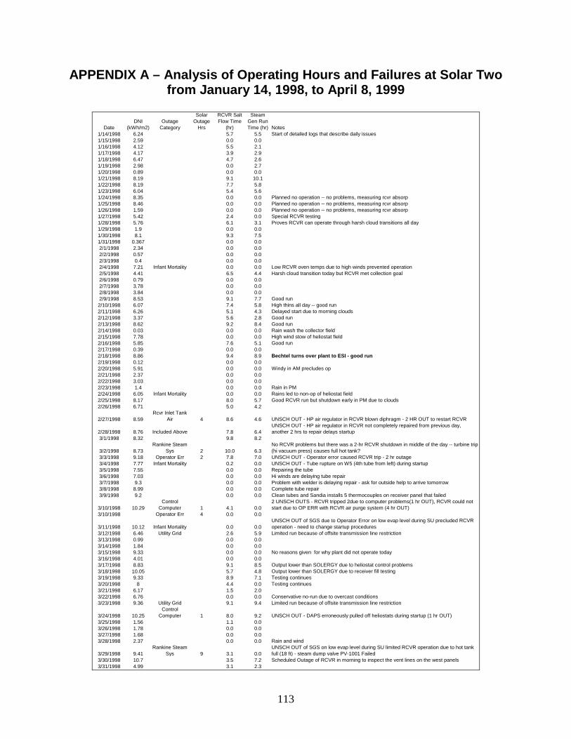
113

APPENDIX A – Analysis of Operating Hours and Failures at Solar Two from January 14, 1998, to April 8, 1999

DateDNI

(kWh/m2)Outage

Category

Solar Outage

Hrs

RCVR Salt Flow Time

(hr)

Steam Gen Run Time (hr) Notes

1/14/1998 6.24 5.7 5.5 Start of detailed logs that describe daily issues1/15/1998 2.59 0.0 0.01/16/1998 4.12 5.5 2.11/17/1998 4.17 3.9 2.91/18/1998 6.47 4.7 2.61/19/1998 2.98 0.0 2.71/20/1998 0.89 0.0 0.01/21/1998 8.19 9.1 10.11/22/1998 8.19 7.7 5.81/23/1998 6.04 5.4 5.61/24/1998 8.35 0.0 0.0 Planned no operation -- no problems, measuring rcvr absorp1/25/1998 8.46 0.0 0.0 Planned no operation -- no problems, measuring rcvr absorp1/26/1998 1.59 0.0 0.0 Planned no operation -- no problems, measuring rcvr absorp1/27/1998 5.42 2.4 0.0 Special RCVR testing1/28/1998 5.76 6.1 3.1 Proves RCVR can operate through harsh cloud transitions all day1/29/1998 1.9 0.0 0.01/30/1998 8.1 9.3 7.51/31/1998 0.367 0.0 0.02/1/1998 2.34 0.0 0.02/2/1998 0.57 0.0 0.02/3/1998 0.4 0.0 0.02/4/1998 7.21 Infant Mortality 0.0 0.0 Low RCVR oven temps due to high winds prevented operation2/5/1998 4.41 6.5 4.4 Harsh cloud transition today but RCVR met collection goal2/6/1998 0.79 0.0 0.02/7/1998 3.78 0.0 0.02/8/1998 3.84 0.0 0.02/9/1998 8.53 9.1 7.7 Good run2/10/1998 6.07 7.4 5.8 High thins all day -- good run2/11/1998 6.26 5.1 4.3 Delayed start due to morning clouds2/12/1998 3.37 5.6 2.8 Good run2/13/1998 8.62 9.2 8.4 Good run2/14/1998 0.03 0.0 0.0 Rain wash the collector field2/15/1998 7.78 0.0 0.0 High wind stow of heliostat field2/16/1998 5.85 7.6 5.1 Good run2/17/1998 0.39 0.0 0.02/18/1998 8.86 9.4 8.9 Bechtel turns over plant to ESI - good run2/19/1998 0.12 0.0 0.02/20/1998 5.91 0.0 0.0 Windy in AM precludes op2/21/1998 2.37 0.0 0.02/22/1998 3.03 0.0 0.02/23/1998 1.4 0.0 0.0 Rain in PM2/24/1998 6.05 Infant Mortality 0.0 0.0 Rains led to non-op of heliostat field2/25/1998 8.17 8.0 5.7 Good RCVR run but shutdown early in PM due to clouds2/26/1998 6.71 5.0 4.2

2/27/1998 8.59Rcvr Inlet Tank

Air 4 8.6 4.6 UNSCH OUT - HP air regulator in RCVR blown diphragm - 2 HR OUT to restart RCVR

2/28/1998 8.76 Included Above 7.8 6.4UNSCH OUT - HP air regulator in RCVR not completely repaired from previous day, another 2 hrs to repair delays startup

3/1/1998 8.32 9.8 8.2

3/2/1998 8.73Rankine Steam

Sys 2 10.0 6.3No RCVR problems but there was a 2-hr RCVR shutdown in middle of the day -- turbine trip (hi vacuum press) causes full hot tank?

3/3/1998 9.18 Operator Err 2 7.8 7.0 UNSCH OUT - Operator error caused RCVR trip - 2 hr outage3/4/1998 7.77 Infant Mortality 0.2 0.0 UNSCH OUT - Tube rupture on W5 (4th tube from left) during startup3/5/1998 7.55 0.0 0.0 Repairing the tube3/6/1998 7.03 0.0 0.0 Hi winds are delaying tube repair3/7/1998 9.3 0.0 0.0 Problem with welder is delaying repair - ask for outside help to arrive tomorrow3/8/1998 8.99 0.0 0.0 Complete tube repair3/9/1998 9.2 0.0 0.0 Clean tubes and Sandia installs 5 thermocouples on receiver panel that failed

3/10/1998 10.29Control

Computer 1 4.1 0.02 UNSCH OUTS - RCVR tripped 2due to computer problems(1 hr OUT), RCVR could not start due to OP ERR with RCVR air purge system (4 hr OUT)

3/10/1998 Operator Err 4 0.0 0.0

3/11/1998 10.12 Infant Mortality 0.0 0.0UNSCH OUT of SGS due to Operator Error on low evap level during SU precluded RCVR operation - need to change startup procedures

3/12/1998 6.46 Utility Grid 2.6 5.9 Limited run because of offsite transmission line restriction3/13/1998 0.99 0.0 0.03/14/1998 1.84 0.0 0.03/15/1998 9.33 0.0 0.0 No reasons given for why plant did not operate today3/16/1998 4.01 0.0 0.03/17/1998 8.83 9.1 8.5 Output lower than SOLERGY due to heliostat control problems3/18/1998 10.05 5.7 4.8 Output lower than SOLERGY due to receiver fill testing3/19/1998 9.33 8.9 7.1 Testing continues3/20/1998 8 4.4 0.0 Testing continues3/21/1998 6.17 1.5 2.03/22/1998 6.76 0.0 0.0 Conservative no-run due to overcast conditions3/23/1998 9.36 Utility Grid 9.1 9.4 Limited run because of offsite transmission line restriction

3/24/1998 10.25Control

Computer 1 8.0 9.2 UNSCH OUT - DAPS erroneously pulled off heliostats during startup (1 hr OUT)3/25/1998 1.56 1.1 0.03/26/1998 1.78 0.0 0.03/27/1998 1.68 0.0 0.03/28/1998 2.37 0.0 0.0 Rain and wind


Sys 9 3.1 0.0UNSCH OUT of SGS on low evap level during SU limited RCVR operation due to hot tank full (18 ft) - steam dump valve PV-1001 Failed

3/30/1998 10.7 3.5 7.2 Scheduled Outage of RCVR in morning to inspect the vent lines on the west panels3/31/1998 4.99 3.1 2.3

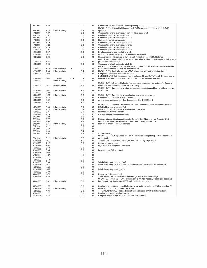
114

4/1/1998 6.32 0.0 0.0 Converative no operation due to many passing clouds

4/2/1998 8.72 Infant Mortality 4.5 3.4UNSCH OUT - Heliostat field burned the RCVR over covers - Lost ~4 hrs of RCVR operation

4/3/1998 4.37 0.0 0.0 Continue to perform oven repair - removed to ground level4/4/1998 6.07 0.0 0.0 Continue to perform oven repair in shop4/5/1998 5.15 0.0 0.0 Continue to perform oven repair in shop4/6/1998 3.12 0.0 0.0 High winds hampers over repair4/7/1998 8.19 0.0 0.0 Continue to perform oven repair in shop4/8/1998 10.23 0.0 0.0 Continue to perform oven repair in shop4/9/1998 9.29 0.0 0.0 Continue to perform oven repair in shop4/10/1998 9.97 0.0 0.0 Continue to perform oven repair in shop4/11/1998 3.97 0.0 0.0 Finishing receiver oven and other work4/12/1998 10.02 0.0 0.0 High Winds all day prevented operation of heliostat field4/13/1998 5.36 0.0 0.0 Receiver returned to service today, but high winds kept heliostat field stowed

4/14/1998 6.84 0.0 0.0Looks like BCS work and winds prevented operation. Perhaps checking aim of heliostats to prevent reburn of ovens?

4/15/1998 8.26 0.0 0.0 Continuing to check heliostats with BCS

4/16/1998 10.3 Heat Trace Sys 9 0.0 0.0UNSCH OUT - Riser plugged - 2 heat trace circuits found off. Perhaps riser strainer was frozen? Soaked riser at 600 F all day to recover.

4/17/1998 9.99 Infant Mortality 0.4 0.0 UNSCH OUT - Small tube leak on W5 (5th tube from left) noticed during startup4/18/1998 10.85 0.0 0.0 Completed tube repair and other misc jobs

4/19/1998 10.26 HVAC 3.25 5.4 0.82 UNSCH OUTS - ILS link caused field to defocus (15 min OUT). Then SG tripped due to cold salt in hot-pump sump (lost 5 hrs of collection because hot tank full)

4/19/1998 Infant Mortality 0.0 0.0

4/20/1998 10.03 Included Above 5.5 8.6UNSCH OUT - ILS tripped heliostat field again (same problem as yesterday). Cause is failure of HVAC in remote station #1 (3 hr OUT)

4/21/1998 10.22 Infant Mortality 1.1 8.8UNSCH OUT - Oven covers are burning again due to aiming problem - shutdown receiver most of day.

4/22/1998 9.93 9.9 13.14/23/1998 10.37 Infant Mortality 2.3 0.0 UNSCH OUT - Oven covers are oveheating due to aiming problem4/24/1998 9.78 0.0 0.0 Continue to troubleshoot aiming problem4/25/1998 4.52 0.0 0.0 Aiming issue semi resolved. See discussion in SAND2002-01204/26/1998 7.81 7.6 6.8

4/27/1998 9.68 Infant Mortality 9.9 6.5UNSCH OUT - Operator error caused SGS trip - procedures were not properly followed. RCVR offline due to hot tank full

4/28/1998 9.23 Infant Mortality 4.4 3.6 UNSCH OUT - Oven covers are oveheating once again4/29/1998 9.35 0.0 0.0 Repaired oven cover brackets4/30/1998 9.26 4.6 3.3 Receiver aimpoint testing continues5/1/1998 9.22 6.2 8.75/2/1998 9.77 0.0 0.0 Receiver aimpoint testing continues by Sandia's Bob Edgar and Ken Stone (MDAC)5/3/1998 9.08 7.5 7.7 Good run but early conservative shutdown due to many puffy clouds5/4/1998 6.75 Infant Mortality 0.0 0.0 High winds precluded RCVR preheat5/5/1998 4.12 0.0 0.05/6/1998 2.73 0.0 0.05/7/1998 4.94 3.4 0.05/8/1998 9.93 2.2 2.7 Aimpoint testing

5/9/1998 8.22 Infant Mortality 3.7 0.0UNSCH OUT - RCVR plugged tube on W5 identified during startup. RCVR operated in preheat only.

5/10/1998 10.01 1.0 0.0 The W5 tube plug ruptured today (5th tube from North). High winds.5/11/1998 7.17 0.0 0.0 Started to replace tube.5/12/1998 3.94 0.0 0.0 High winds are hampering tube repair5/13/1998 3.43 0.0 0.05/14/1998 9.35 0.0 0.0 Lowered panel W5 to ground5/15/1998 10.44 0.0 0.05/16/1998 8.82 0.0 0.05/17/1998 11.01 0.0 0.05/18/1998 9.58 0.0 0.05/19/1998 8.33 0.0 0.0 Winds hampering reinstall of W55/20/1998 10.07 0.0 0.0 Winds hampering reinstall of W5 - start to schedule 430 am work to avoid winds5/21/1998 11.33 0.0 0.05/22/1998 10.95 0.0 0.0 Winds in morning slowing work5/23/1998 9.93 0.0 0.05/24/1998 10.36 0.0 0.0 Receiver repairs completed5/25/1998 7.26 0.0 0.7 Spent most of the day reheating the steam generator after long outage

5/26/1998 6.62 Infant Mortality 0.0 0.0UNSCH OUT? See 7/8 - RCVR bypass valve (HV5020) heat trace cable and spare are both burned out. Don't start RCVR until fixed - Conservative?.

5/27/1998 11.05 0.0 0.0 Installed new heat trace. Used heliostats to try and thaw a plug in W8 first noted on 5/95/28/1998 9.52 Infant Mortality 0.0 0.0 UNSCH OUT - Could not thaw plug in W85/29/1998 4.06 0.0 0.0 Too windy to thaw W8 - decide to install new heat trace on W8 to help with thaw5/30/1998 11.03 0.0 0.0 Installed heat trace to help with thaw5/31/1998 7.48 0.0 0.0 Complete install of heat trace and test W8 temperatures

115

6/1/1998 11.12 Rcvr Trip - Unk 1.5 7.3 5.5 UNSCH OUT - Receiver trip, cause unknown (OUT 1.5 hrs). Tube thawed mid day

6/2/1998 10.82Steam Gen Trip - Unk 4 4.5 7.7 UNSCH OUT - SGS tripped (cause unknown). Hot Tank full thus trip receiver. (OUT ~4hrs)

6/3/1998 9.48 0.0 0.0 High winds during preheat and then stowed field rest of day 6/4/1998 10.83 9.1 11.8 Several tube plugs on W6 delayed startup until mid day.6/5/1998 10.63 Rcvr Trip - Unk 2 9.6 13.3 UNSCH OUT - 2 Receiver ILS trips (unknown cause) (OUT 2 hr)

6/6/1998 9.42 8.3 13.9Station blackout during night (when SGS operating?). Safely shutdown systems. Wind caused.

6/7/1998 10.54Helio Field

Common Mode 10 0.0 0.0UNSCH OUT - Last nights blackout caused many heliostat control strings to fail. All day to recover.

6/8/1998 8.94 7.6 15.6

6/9/1998 8.8Rcvr Panel

Drain Valves 3 6.7 7.2UNSCH OUT - RCVR drain valve solenoid failure delayed startup (gummed up, clean/reinstall) (OUT 3 hrs)

6/10/1998 5.59Control

Computer 0.5 6.1 9.2 UNSCH OUT - ILS trip (unknown) (OUT 30 min)6/11/1998 10.12 0.0 0.0 Scheduled Outage to install to replace RCVR ball valves with gate valves6/12/1998 7.21 0.0 0.0 Tried to test new gates valves but clouds hampered test6/13/1998 11.01 10.2 14.1 First ever SGS run through the night

6/14/1998 10.98Control

Computer 1 9.7 24.0UNSCH OUT - Master Control Computer failed delaying RCVR startup, needed to reboot (OUT 1 hr)

6/15/1998 10.43 11.6 24.0 Good run6/16/1998 10.41 Infant Mortality 2.5 9.4 UNSCH OUT - Several plugged tubes in W8 - high winds. Ended ~70 hr SGS run.

6/17/1998 11.64 6.6 4.5Plugs cleared but SU delayed to repair air tank to reduce air consumption - could have done this repair at night?

6/18/1998 11.32 13.1 16.6 Good run

6/19/1998 11.26 Infant Mortality 6.4 3.2UNSCH OUT see 7/8? - RCVR bypass valve (HV5020) heat trace cable and spare are both burned out. Delayed startup (4hrs) of RCVR (conservative decision?) -ordered cables

6/20/1998 11.16 12.3 15.3 Good run6/21/1998 11.61 Infant Mortality 10.9 9.6 UNSCH OUT - RCVR plug in W5 delayed startup by 2 hr

6/22/1998 11.5 Heat Trace Sys 9 0.0 0.0UNSCH OUT - Inlet tank vent valve (PV5003) obstructed with salt - cleaned and stoked (OUT 9hrs) valve heat trace failure??

6/23/1998 11.25 Infant Mortality 11.5 15.0UNSCH OUT - RCVR plug in W7 with 25 mph wind delayed startup ~2 hr. Removed PV5003 after run and found plug in pipe, not valve

6/24/1998 10.88 8.6 9.7 Dispatchability testing (25%, 50%, 75%)6/25/1998 10.8 Infant Mortality 1.9 0.0 UNSCH OUT - RCVR plug in W7 on SU with high winds - no run6/26/1998 11.08 10.2 9.8 Good run6/27/1998 11.22 9.4 11.5 Dispatchability test6/28/1998 11.54 8.7 12.4 Dispatchability test6/29/1998 11.41 Infant Mortality 11.1 15.9 UNSCH OUT - RCVR plug delayed SU by ~30 minutes6/30/1998 11.2 Infant Mortality 4.2 14.4 UNSCH OUT - RCVR plug delayed SU until afternoon7/1/1998 11.12 Infant Mortality 11.7 16.8 UNSCH OUT - RCVR plug delayed SU a few hours7/2/1998 10.79 Infant Mortality 12.3 24.0 UNSCH OUT - RCVR plug delayed SU ~2 hours7/3/1998 10.83 12.5 24.0 Good run7/4/1998 11.05 12.2 24.0 Good run


Air 1 11.0 24.0UNSCH OUT - Unknown problem caused spill through inlet tank vent (OUT 1 hr) - supect inlet tank air valve malfunction

7/6/1998 9.4 11.5 24.4 Good run7/7/1998 7.52 9.0 18.87/8/1998 7.76 9.2 9.3 HV5020 thermocouple connection failed but did not impact operation


Sys 1.5 11.2 8.5 UNSCH OUT - Turbine control problem caused SU failure. Hot tank full (OUT 1.5 hr)7/10/1998 11.08 Infant Mortality 11.4 14.9 UNSCH OUT - RCVR plug on W7 delayed SU ~2 hours

7/11/1998 11.86 Infant Mortality 9.2 0.0UNSCH OUT - RCVR plug on W5 prevented operation - cold tank was heated to 600 F due to salt circulation

7/12/1998 11.94 Infant Mortality 9.1 8.7 UNSCH OUT - RCVR plug on W5 delayed SU ~3 hours7/13/1998 11.86 Infant Mortality 12.1 11.1 UNSCH OUT - RCVR plug on W7 delayed SU ~0.5 hours

7/14/1998 11.41Steam Gen Water Pump 4 11.4 7.9

UNSCH OUT - SGS water pump P853 tripped 2 times on hi temperature. Hot Tank full. (OUT 4 hr)


Sys 4 7.6 8.0UNSCH OUT - Turbine tripped. Exhaust instrument recalibration fixed the problem (OUT 4 hr)

7/16/1998 10.77 Salt FCVs 15 0.0 0.0 UNSCH OUT - Repair salt valve leak (PSV5071) piping (cold pump recirc line) - out all day

7/17/1998 8.72 Included Above 1.8 0.0UNSCH OUT - Complete repair of PSV5071 - reheat the valve with heat trace. Total OUT was 15 hrs.

7/18/1998 7.15 8.2 4.0 Firecracker 250 race puts much dust in the air

7/19/1998 7.1Maintenance

Err 10 0.0 0.0UNSCH OUT - PV5003 Inlet Tank Vent Valve did not close during morning fill. Operations found no problem but nightshift found valve open. (OUT 10 hr)

7/20/1998 1.83 0.0 0.0


Air 4 4.6 1.8 UNSCH OUT - Inlet tank pressure control failed (OUT 4 hr)7/22/1998 4.59 0.0 0.0 SCHED OUT - Inspecting/cleaning internals of SGS Preheater.

7/23/1998 6.96 0.0 0.0SGS outage continues. Much other work being done, e.g. cold pump motors were sent off site

7/24/1998 10.34 0.0 0.07/25/1998 10.92 0.0 0.07/26/1998 11.06 0.0 0.07/27/1998 10.63 0.0 0.0 Inspected Evaporator today. Took many days to cool down the kettle.

7/28/1998 8.75 0.0 0.0Evaporator temperature and pressure coming up slowly. Emergency diesel failed several start attempts

7/29/1998 10.56 0.0 2.3 Testing SGS after heating up. Outage ends.7/30/1998 11.19 4.4 1.4 Short run today but no report is available to explain why


Air 4 8.2 13.3UNSCH OUT - Late start - looks like to adjust inlet vessel vent valve PV5003 to ensure tight closure

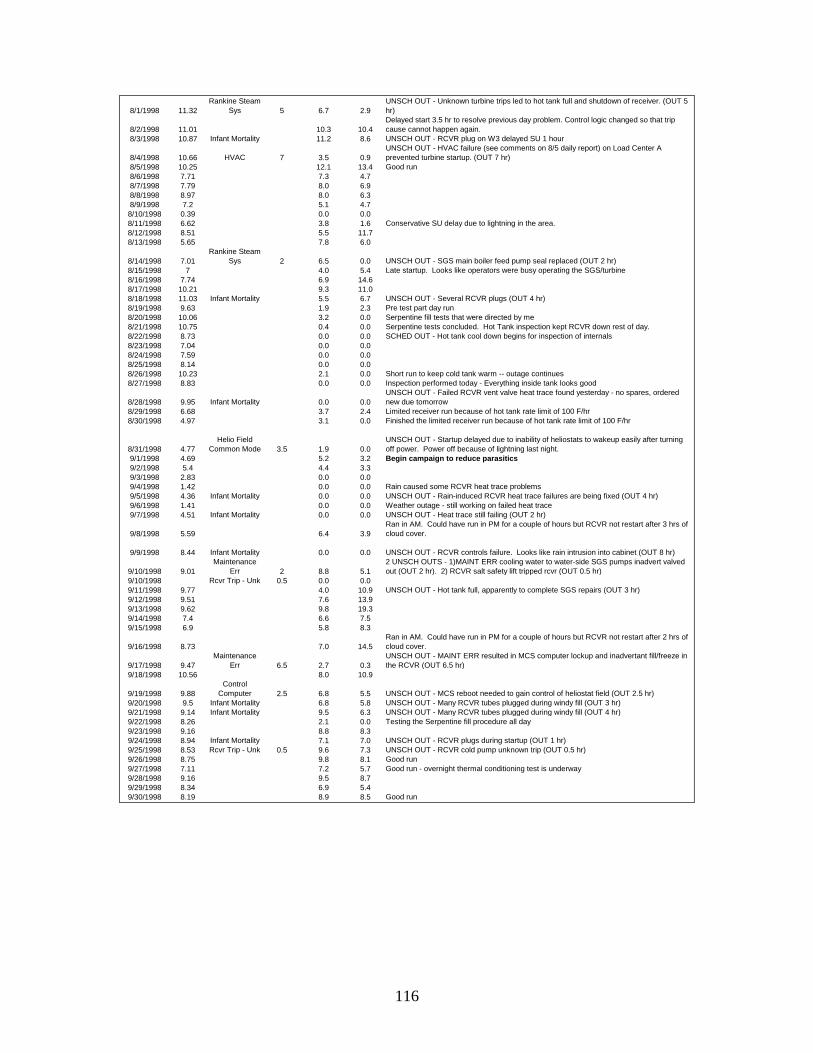
116


Sys 5 6.7 2.9UNSCH OUT - Unknown turbine trips led to hot tank full and shutdown of receiver. (OUT 5 hr)

8/2/1998 11.01 10.3 10.4Delayed start 3.5 hr to resolve previous day problem. Control logic changed so that trip cause cannot happen again.

8/3/1998 10.87 Infant Mortality 11.2 8.6 UNSCH OUT - RCVR plug on W3 delayed SU 1 hour

8/4/1998 10.66 HVAC 7 3.5 0.9UNSCH OUT - HVAC failure (see comments on 8/5 daily report) on Load Center A prevented turbine startup. (OUT 7 hr)

8/5/1998 10.25 12.1 13.4 Good run8/6/1998 7.71 7.3 4.78/7/1998 7.79 8.0 6.98/8/1998 8.97 8.0 6.38/9/1998 7.2 5.1 4.78/10/1998 0.39 0.0 0.08/11/1998 6.62 3.8 1.6 Conservative SU delay due to lightning in the area.8/12/1998 8.51 5.5 11.78/13/1998 5.65 7.8 6.0


Sys 2 6.5 0.0 UNSCH OUT - SGS main boiler feed pump seal replaced (OUT 2 hr)8/15/1998 7 4.0 5.4 Late startup. Looks like operators were busy operating the SGS/turbine8/16/1998 7.74 6.9 14.68/17/1998 10.21 9.3 11.08/18/1998 11.03 Infant Mortality 5.5 6.7 UNSCH OUT - Several RCVR plugs (OUT 4 hr)8/19/1998 9.63 1.9 2.3 Pre test part day run8/20/1998 10.06 3.2 0.0 Serpentine fill tests that were directed by me8/21/1998 10.75 0.4 0.0 Serpentine tests concluded. Hot Tank inspection kept RCVR down rest of day.8/22/1998 8.73 0.0 0.0 SCHED OUT - Hot tank cool down begins for inspection of internals8/23/1998 7.04 0.0 0.08/24/1998 7.59 0.0 0.08/25/1998 8.14 0.0 0.08/26/1998 10.23 2.1 0.0 Short run to keep cold tank warm -- outage continues8/27/1998 8.83 0.0 0.0 Inspection performed today - Everything inside tank looks good

8/28/1998 9.95 Infant Mortality 0.0 0.0UNSCH OUT - Failed RCVR vent valve heat trace found yesterday - no spares, ordered new due tomorrow

8/29/1998 6.68 3.7 2.4 Limited receiver run because of hot tank rate limit of 100 F/hr8/30/1998 4.97 3.1 0.0 Finished the limited receiver run because of hot tank rate limit of 100 F/hr

8/31/1998 4.77Helio Field

Common Mode 3.5 1.9 0.0UNSCH OUT - Startup delayed due to inability of heliostats to wakeup easily after turning off power. Power off because of lightning last night.

9/1/1998 4.69 5.2 3.2 Begin campaign to reduce parasitics9/2/1998 5.4 4.4 3.39/3/1998 2.83 0.0 0.09/4/1998 1.42 0.0 0.0 Rain caused some RCVR heat trace problems9/5/1998 4.36 Infant Mortality 0.0 0.0 UNSCH OUT - Rain-induced RCVR heat trace failures are being fixed (OUT 4 hr) 9/6/1998 1.41 0.0 0.0 Weather outage - still working on failed heat trace9/7/1998 4.51 Infant Mortality 0.0 0.0 UNSCH OUT - Heat trace still failing (OUT 2 hr)

9/8/1998 5.59 6.4 3.9Ran in AM. Could have run in PM for a couple of hours but RCVR not restart after 3 hrs of cloud cover.

9/9/1998 8.44 Infant Mortality 0.0 0.0 UNSCH OUT - RCVR controls failure. Looks like rain intrusion into cabinet (OUT 8 hr)


Err 2 8.8 5.12 UNSCH OUTS - 1)MAINT ERR cooling water to water-side SGS pumps inadvert valved out (OUT 2 hr). 2) RCVR salt safety lift tripped rcvr (OUT 0.5 hr)

9/10/1998 Rcvr Trip - Unk 0.5 0.0 0.09/11/1998 9.77 4.0 10.9 UNSCH OUT - Hot tank full, apparently to complete SGS repairs (OUT 3 hr) 9/12/1998 9.51 7.6 13.99/13/1998 9.62 9.8 19.39/14/1998 7.4 6.6 7.59/15/1998 6.9 5.8 8.3

9/16/1998 8.73 7.0 14.5Ran in AM. Could have run in PM for a couple of hours but RCVR not restart after 2 hrs of cloud cover.


Err 6.5 2.7 0.3UNSCH OUT - MAINT ERR resulted in MCS computer lockup and inadvertant fill/freeze in the RCVR (OUT 6.5 hr)

9/18/1998 10.56 8.0 10.9

9/19/1998 9.88Control

Computer 2.5 6.8 5.5 UNSCH OUT - MCS reboot needed to gain control of heliostat field (OUT 2.5 hr)9/20/1998 9.5 Infant Mortality 6.8 5.8 UNSCH OUT - Many RCVR tubes plugged during windy fill (OUT 3 hr)9/21/1998 9.14 Infant Mortality 9.5 6.3 UNSCH OUT - Many RCVR tubes plugged during windy fill (OUT 4 hr)9/22/1998 8.26 2.1 0.0 Testing the Serpentine fill procedure all day9/23/1998 9.16 8.8 8.39/24/1998 8.94 Infant Mortality 7.1 7.0 UNSCH OUT - RCVR plugs during startup (OUT 1 hr)9/25/1998 8.53 Rcvr Trip - Unk 0.5 9.6 7.3 UNSCH OUT - RCVR cold pump unknown trip (OUT 0.5 hr)9/26/1998 8.75 9.8 8.1 Good run9/27/1998 7.11 7.2 5.7 Good run - overnight thermal conditioning test is underway9/28/1998 9.16 9.5 8.79/29/1998 8.34 6.9 5.49/30/1998 8.19 8.9 8.5 Good run

117

10/1/1998 9.32Control

Computer 1 4.1 5.12 UNSCH OUTS - 1) MCS lockup delayed RCVR SU (OUT 1 hr) 2) Main steam bypass valve erratic causes SGS trip (OUT 4 hr)

10/1/1998Rankine Steam

Sys 4 0.0 0.010/2/1998 9.55 9.0 8.910/3/1998 8.45 Infant Mortality 0.0 0.0 UNSCH OUT - high winds preclude RCVR preheat - cold ovens10/4/1998 9.11 Infant Mortality 9.6 7.7 UNSCH OUT - plugged tubes during RCVR SU (OUT 2 hr)10/5/1998 9.84 HVAC 2 7.0 7.0 UNSCH OUT - RCVR remote station HVAC problem delayed SU (OUT 2 hr)10/6/1998 9.25 10.7 9.0 Good run10/7/1998 6.73 9.9 7.9 Outstanding demonstration of energy collection during difficult cloud conditions10/8/1998 8.54 9.9 8.9 Good run10/9/1998 9.19 9.4 8.9 Good run10/10/1998 9.13 Infant Mortality 8.5 7.2 UNSCH OUT - plugged tubes during RCVR SU (OUT 2 hr)10/11/1998 8.18 Infant Mortality 9.5 7.7 UNSCH OUT - plugged tubes during RCVR SU (OUT 0.5 hr)10/12/1998 5.61 5.8 6.0 Good run10/13/1998 8.61 9.6 7.8 Good run10/14/1998 6.63 Infant Mortality 6.1 0.0 UNSCH OUT - plugged tubes during RCVR SU (OUT 2 hr)10/15/1998 6.67 Infant Mortality 0.0 0.0 UNSCH OUT - high winds preclude RCVR preheat - cold ovens

10/16/1998 8.13 Rcvr Trip - Unk 3 4.8 7.9UNSCH OUT - RCVR tripped due to erroneous salt flow transmitter, but no problem found (OUT 3 hr)

10/17/1998 8.96 10.2 5.810/18/1998 8.85 10.0 8.2 Good run

10/19/1998 8.01Control

Computer 2 7.9 7.3 UNSCH OUT - MCS anomaly delayed SU of RCVR (OUT 2 hr)10/20/1998 8.28 10.0 9.0 Good run

10/21/1998 8.3 Salt FCVs 1 8.3 7.4UNSCH OUT - RCVR flow control valve 5302A problem. Adjust and continue SU. B valve is not auto backup. (OUT 2 hr)

10/22/1998 9.32 0.0 0.0SCHED OUT - Installing heat trace on lower tube clip area to mitigate plugged tube problem W3, W5, W7

10/23/1998 7.07 0.0 0.0 Outage continues - 24 hr average parasitic power is reduced to 416 kW10/24/1998 1.76 2.1 0.0 Receiver ran on a bad weather day10/25/1998 6.48 7.1 7.1 Good run10/26/1998 7.42 6.1 4.5

10/27/1998 8.36 0.0 0.0SCHED OUT - Installing heat trace on lower tube clip area to mitigate plugged tube problem W4, W6, W8,

10/28/1998 7.37 0.0 0.0 Outage continues - 24 hr average parasitic power is 446 kW 10/29/1998 2.91 0.0 0.010/30/1998 3.21 0.0 0.0

10/31/1998 8.91 Infant Mortality 2.5 5.1 0.7UNSCH OUT - RCVR Backtube TC fails causing RCVR trip lock in -Heliostats would not go to preheat (OUT 2.5 hr). Remove TC from scan.

11/1/1998 7.76 7.7 13.611/2/1998 6.6 8.7 6.6 Good run11/3/1998 8.27 9.7 8.0 Good run11/4/1998 7.69 9.3 7.8 Good run11/5/1998 7.25 Infant Mortality 8.2 4.0 UNSCH OUT - plugged tubes in W5, W7 during RCVR SU (OUT 4.5 hr)11/6/1998 7.79 Infant Mortality 8.8 7.4 UNSCH OUT - plugged tubes during RCVR SU (OUT 0.5 hr)11/7/1998 5.96 Infant Mortality 0.0 0.0 UNSCH OUT - high winds preclude RCVR preheat - too cold to fill11/8/1998 4.06 0.0 0.011/9/1998 7.37 Infant Mortality 4.7 4.4 UNSCH OUT - plugged tubes (W4, W5, W6, W7) during RCVR SU (OUT 2 hr)11/10/1998 7.19 5.1 5.411/11/1998 0.33 0.0 0.011/12/1998 8.57 8.8 7.2 Receiver efficiency test run today11/13/1998 8.51 6.6 5.4 Receiver efficiency test run today11/14/1998 8.6 0.0 0.0 No run today (Weekend) lack of manpower11/15/1998 8.13 0.0 0.0 No run today (Weekend) lack of manpower11/16/1998 6.57 Infant Mortality 1.2 0.0 UNSCH OUT - DOWNCOMER RUPTURED

0.0 0.02/23/1999 8.67 3.8 0.0 Short receiver run after returning from long outage2/24/1999 7.42 3.6 2.5 Short run with many restart problems that were resolved2/25/1999 7.45 6.3 4.8

2/26/1999 8.18 Salt FCVs 8 2.6 0.0UNSCH OUT - Flow control problems in RCVR (OUT 8 hr), SEGS 1 Storage System destroyed today.

2/27/1999 8.2 0.0 0.0 Budget prohibits run on weekend - Smoke from SEGS 1 fire2/28/1999 8 0.0 4.5 Budget prohibits run on weekend - Ran SGS to get ready for Monday run

118

3/1/1999 7.63 8.3 5.2 Receiver efficiency test. Defocussing lead to an E that is 75% of SOLERGY3/2/1999 8.38 10.2 8.8 Receiver efficiency test. Defocussing lead to an E that is 90% of SOLERGY

3/3/1999 8.54 5.6 4.8 Receiver drain/fill test in high winds - Receiver did not meet refill temperature requirements

3/4/1999 8.93 Infant Mortality 8.1 3.9UNSCH OUT - High AM winds caused numerous RCVR plugs on SU -- W4, 5, 7, and 8 (OUT 3 hr)

3/5/1999 9.56 Infant Mortality 9.9 8.3UNSCH OUT - High AM winds caused RCVR plugs (OUT 1 hr), Receiver efficiency testing continues

3/6/1999 7.09 0.0 0.0 Budget prohibits run on weekend 3/7/1999 6.63 0.0 0.0 Budget prohibits run on weekend


Air 7 3.0 0.0UNSCH OUT - Air inlet valve to inlet vessel. Valve OK but no signal to computers (OUT 7 hr)


Level Inst 3 1.5 3.2 UNSCH OUT - Nuclear level detector for inlet vessel repaired and calibrated (OUT 3 hr)3/10/1999 5.66 Rcvr Trip - Unk 0.5 6.5 3.9 UNSCH OUT - 2 RCVR trips for unknown reasons (OUT 0.5 hr)3/11/1999 5.9 2.7 0.0 Receiver fill and drain tests during cloudy/windy weather - good results3/12/1999 8.41 10.4 9.5 Receiver efficiency test. Defocussing lead to an E that is 85% of SOLERGY3/13/1999 7.41 0.0 0.0 Budget prohibits run on weekend3/14/1999 2.74 0.0 0.0 Budget prohibits run on weekend3/15/1999 5.67 0.0 0.0 High winds and clouds prevented operation3/16/1999 1.05 0.0 0.03/17/1999 9.31 10.0 8.3 Receiver efficiency test. Defocussing lead to an E that is 85% of SOLERGY3/18/1999 8.23 9.6 9.4 Receiver efficiency test. Defocussing lead to an E that is 89% of SOLERGY3/19/1999 2.82 0.0 0.0 Performed some scheduled maintenance during bad weather3/20/1999 9.77 0.0 0.0 Budget prohibits run on weekend3/21/1999 9.38 0.0 0.0 Budget prohibits run on weekend3/22/1999 7.88 8.1 8.3 Receiver efficiency test. Defocussing lead to an E that is 75% of SOLERGY3/23/1999 8.43 9.4 9.5 Receiver efficiency test. Defocussing lead to an E that is 75% of SOLERGY3/24/1999 8.41 9.4 10.7 Receiver efficiency test. Defocussing lead to an E that is 82% of SOLERGY3/25/1999 0.14 0.0 0.0

3/26/1999 9.04 Infant Mortality 4.2 2.0UNSCH OUT - Operator Error led to SGS trip - Conservative shutdown since turbine insulation is soaked with oil (OUT 6 hr)

3/27/1999 9.35 1.0 6.7Budget prohibits run on weekend - but running turbine in steam dump mode because of oil in insulation

3/28/1999 8.01 0.0 0.0 Budget prohibits run on weekend

3/29/1999 8.41Control

Computer 1 9.7 8.9UNSCH OUT - Receiver tripped 2 time due to ILS problems (OUT 1 hr). Turbine idle due to oil. E is 86% of SOLERGY.

3/30/1999 7.7 9.1 8.9Receiver efficiency test. Defocussing lead to an E that is 75% of SOLERGY. Turbine idle due to oil.

3/31/1999 3.75 0.0 0.0 Weather outage. Winds ~ 50 mph.4/1/1999 5.82 6.2 6.3 Receiver testing. E is 94% of SOLERGY.

4/2/1999 9.47 0.3 0.0Receiver test. Studied the discharge of the inlet tank during blackout conditions with no RCVR pump. Looks good.

4/3/1999 2.33 0.0 0.0 Budget prohibits run on weekend4/4/1999 5.05 0.0 0.0 Budget prohibits run on weekend4/5/1999 8.77 4.3 0.0 Short run. No daily report to say why.4/6/1999 1.33 0.0 0.04/7/1999 6.96 1.8 0.0 Receiver blackout test. Looks good. 4/8/1999 8.21 11.4 9.2 Ran aimpoint test for T&E group. RCVR shut down for last time at 7 pm.

1460 1474

119

DISTRIBUTION Internal distribution (distributed electronically unless otherwise noted): 1 MS0899 RIM-Reports Management 9532 (electronic copy)

120