HAL Id: hal-01136715https://hal.archives-ouvertes.fr/hal-01136715

Submitted on 27 Mar 2015

HAL is a multi-disciplinary open accessarchive for the deposit and dissemination of sci-entific research documents, whether they are pub-lished or not. The documents may come fromteaching and research institutions in France orabroad, or from public or private research centers.

L’archive ouverte pluridisciplinaire HAL, estdestinée au dépôt et à la diffusion de documentsscientifiques de niveau recherche, publiés ou non,émanant des établissements d’enseignement et derecherche français ou étrangers, des laboratoirespublics ou privés.

An evaluation metric for intraseasonal variability and itsapplication to CMIP3 twentieth-century simulations

Prince Xavier, Jean-Philippe Duvel, Pascale Braconnot, F.J. Doblas-Reyes

To cite this version:Prince Xavier, Jean-Philippe Duvel, Pascale Braconnot, F.J. Doblas-Reyes. An evaluation metricfor intraseasonal variability and its application to CMIP3 twentieth-century simulations. Journal ofClimate, American Meteorological Society, 2010, 23 (13), pp.3497-3508. �10.1175/2010JCLI3260.1�.�hal-01136715�

An Evaluation Metric for Intraseasonal Variability and its Applicationto CMIP3 Twentieth-Century Simulations

PRINCE K. XAVIER* AND JEAN-PHILIPPE DUVEL

Laboratoire de Meteorologie Dynamique, Ecole Normale Superieure, Paris, France

PASCALE BRACONNOT

Laboratoire des Sciences du Climat et de l’Environnement, Gif-sur-Yvette, France

FRANCISCO J. DOBLAS-REYES

European Centre for Medium-Range Weather Forecasts, Reading, United Kingdom

(Manuscript received 26 May 2009, in final form 5 February 2010)

ABSTRACT

The intraseasonal variability (ISV) is an intermittent phenomenon with variable perturbation patterns. To

assess the robustness of the simulated ISV in climate models, it is thus interesting to consider the distribution

of perturbation patterns rather than only one average pattern. To inspect this distribution, the authors first

introduce a distance that measures the similarity between two patterns. The reproducibility (realism) of the

simulated intraseasonal patterns is then defined as the distribution of distances between each pattern and

the average simulated (observed) pattern. A good reproducibility is required to analyze the physical source of

the simulated disturbances. The realism distribution is required to estimate the proportion of simulated events

that have a perturbation pattern similar to observed patterns. The median value of this realism distribution is

introduced as an ISV metric. The reproducibility and realism distributions are used to evaluate boreal

summer ISV of precipitations over the Indian Ocean for 19 phase 3 of the Coupled Model Intercomparison

Project (CMIP3) models. The 19 models are classified in increasing ISV metric order. In agreement with

previous studies, the four best ISV metrics are obtained for models having a convective closure totally or

partly based on the moisture convergence. Models with high metric values (poorly realistic) tend to give

(i) poorly reproducible intraseasonal patterns, (ii) rainfall perturbations poorly organized at large scales,

(iii) small day-to-day variability with overly red temporal spectra, and (iv) less accurate summer monsoon

rainfall distribution. This confirms that the ISV is an important link in the seamless system that connects

weather and climate.

1. Introduction

The intraseasonal variability (ISV) of tropical convec-

tion is characterized by large-scale organized perturba-

tions with maximum amplitudes over the Indo-Pacific

region. In boreal winter, they propagate eastward from

the western Indian Ocean to the central Pacific and are

generally referred to as the Madden–Julian oscillation

(MJO) (Madden and Julian 1994). The character of ISV

in boreal summer over the Indian Ocean (see Goswami

2005 for a review) is rather distinct. It initiates around 58S

in the eastern Indian Ocean and propagates northeast-

ward with a speed of about 18 latitude per day. With typical

periods of 30–40 days, these propagating rainbands reach

up to 258N and contribute largely to the rainfall over India.

The summer ISV shows marked seasonality in accordance

with the large seasonal variations of the intertropical con-

vergence zone (ITCZ) over the Indian monsoon region

(Bellenger and Duvel 2007). The strong convective ISV

center is over the eastern equatorial Indian Ocean in May

and shifts to the Arabian Sea (along the west coast of

India) and to the Bay of Bengal in June. The ISV variance

patterns persist for the rest of the monsoon period (July,

* Current affiliation: Met Office Hadley Centre, Exeter, United

Kingdom.

Corresponding author address: Prince K. Xavier, Met Office

Hadley Centre, FitzRoy Road, Exeter EX1 3PB, United Kingdom.

E-mail: prince.xavier@metoffice.gov.uk

1 JULY 2010 X A V I E R E T A L . 3497

DOI: 10.1175/2010JCLI3260.1

� 2010 American Meteorological Society

August, and September) but with a reduced amplitude.

This seasonality in the ISV is intimately related to the

ocean thermal structure and atmosphere–ocean feedbacks

(Xavier et al. 2008; Bellenger and Duvel 2007; Duvel and

Vialard 2007). The ISV is an important component of the

Asian summer monsoon system that can modulate the

synoptic weather systems (Goswami et al. 2003) and

contribute to the seasonal rainfall and its interannual

variability (e.g., Goswami et al. 2006). Therefore, the ac-

curate representation of the ISV in climate models is im-

portant for monsoon forecasting at a range of time scales.

The representation of the ISV in general circulation

models (GCMs) has always been a challenge, primarily

due to its strong dependence on the physical parameter-

izations (Lin et al. 2008, 2006; Waliser et al. 2003; Sperber

et al. 2001; Slingo et al. 1996). In a recent study Xavier

et al. (2008) assess the representation of summer ISV over

the Indian Ocean in the European climate models par-

ticipating in the Development of a European Multimodel

Ensemble System for Seasonal-to-Interannual Prediction

(DEMETER) project. Importantly, the lack of large-scale

organization of convection was regarded as a major cause

of the poor representation of ISV in the DEMETER

models. Lin et al. (2008) analyzed the summer ISV repre-

sented in 14 Intergovernmental Panel on Climate Change

(IPCC) Fourth Assessment Report (AR4) models (sec-

tion 2) and found that the models show a wide range of

skill in the representation of summer ISV, often with

reduced amplitudes and overreddened spectra.

Most of these studies have employed methodologies

based either on empirical orthogonal functions (EOFs),

lead–lag correlations, composites or wavenumber–

frequency spectral analysis (Wheeler and Weickmann

2001). Xavier et al. (2008) have shown that, while the use

of an average EOF (or composites) for a season may be

robust in the observations, caution should be taken on

such a priori assumptions on the robustness of the sim-

ulated ISV. As suggested in Goulet and Duvel (2000,

hereafter GD2000), for an intermittent phenomenon with

large differences between events, the use of a few EOFs

or a single composite might result in quantities that are

pure mathematical without much physical significance.

Lin et al. (2008) present an evaluation of the relative

amplitudes of northward wavenumbers (extracted using

wavenumber–frequency spectra between 458S and 458N

with constraints on the meridional periodicity). The lead–

lag correlations that they have used to compare the north-

ward propagation of rainfall anomalies in the models

pertain to the issue of whether the intraseasonal events

are reproducible in the models. The Climate Variability

and Predictability (CLIVAR) MJO working group has

developed a set of diagnostics that are based on re-

projection of actual outgoing longwave radiation (OLR)

and wind signals on a couple of observed EOFs (Wheeler

and Hendon 2004). Using this index on a GCM simula-

tion output will extract the time evolution of the so-defined

MJO signal, but with no precise information on the GCM

representation of the intraseasonal perturbation patterns.

Moreover, these diagnostics are specifically designed for

zonally propagating intraseasonal perturbations confined

between 158S and 158N. Therefore, the poleward propa-

gating monsoon ISV during boreal summer is not accu-

rately diagnosed with the Wheeler and Hendon index.

An eventwise approach for the assessment of the tropical

ISV in the climate models was first introduced by Xavier

et al. (2008). This method is based on local mode anal-

ysis (LMA) originally developed by GD2000. It provides

the amplitude, phase, degree of large-scale organization,

and period of each organized convective ISV event. The

associated characteristics in other fields such as the sea

surface temperature and winds can also be derived from

this analysis technique.

The objective of this study is to evaluate two major as-

pects of the intermittent ISV, namely, (i) the reproduc-

ibility of the pattern of intraseasonal events and (ii) their

degree of realism. Based on these diagnostics an evalua-

tion metric is defined that can objectively evaluate the ISV

in different models and potentially assess the role of dif-

ferent model physics in the representation of the ISV. A

brief description of the climate models and observations is

given in section 2. The LMA results of summer ISV in

phase 3 of the Coupled Model Intercomparison Project

(CMIP3) are described in section 3. Based on the LMA,

measures of the reproducibility and degree of realism of

the large-scale organized perturbation patterns of ISV are

defined in section 4 and a model evaluation metric is

presented. This metric is applied to evaluate the relation-

ship between high frequency variability and the seasonal

mean rainfall climate in the models (section 5) and results

are summarized in section 6.

2. Models and data

Major international modeling centers have performed

long-term simulations of the twentieth-century climate in

order to better assess their representation of the present-

day climate in preparation for the twenty-first-century

climate sensitivity experiments for the IPCC fourth As-

sessment Report. Most of the modeling centers used the

latest versions of their models, which incorporate state-

of-the-art research results. These include, for example, im-

plementation of prognostic cloud microphysics schemes,

different triggering and closure solutions, and the consid-

eration of some processes such as convective momentum

transport in deep convection schemes. Moreover, many

modeling centers increased their model horizontal and

3498 J O U R N A L O F C L I M A T E VOLUME 23

vertical resolutions and some conducted experiments with

different resolutions. Therefore, it is of interest to assess

the ISV simulations in these new generation climate models

to look at the effects of the updated physical processes,

higher resolution, and air–sea coupling. Such an evalu-

ation is also important for evaluating the general per-

formance of the climate models used for climate change

projections in the IPCC AR4. The model outputs are

archived in the CMIP3 multimodel database at the Pro-

gram for Climate Model Diagnosis and Intercomparison

(PCMDI). The details of the horizontal resolution, clo-

sure, and trigger of different convective schemes in 19

climate IPCC AR4 models are summarized from the

IPCC AR4 (http://www.ipcc-data.org/ar4/gcm_data.html)

and are listed in Table 1. Daily rainfall data from the

models are used for the computation of ISV. Observed

rainfall ISV is derived from the 18-daily (1DD) data of

the Global Precipitation Climatology Project (GPCP)

(Huffman et al. 2001). The rainfall in most models

covers a period of 40 years, while the 1DD GPCP data

is for the period 1997–2006.

3. Local mode analysis of summer ISV

The intraseasonal variability of deep convection over

the Indo-Pacific region is an intermittent phenomenon

presenting various perturbation patterns depending mostly,

but not uniquely, on season. Owing to the relatively long

periodicity of the perturbation (around 40 days) in regard

to the seasonal evolution of the ITCZ, two perturba-

tions succeeding one another in time are rarely simi-

lar (GD2000). However, as shown in Duvel and Vialard

(2007) and in the following, the observed perturbation

pattern for a given season is quite reproducible from one

event to another if one considers only a given basin (i.e.,

the Indian Ocean basin) instead of the whole Indo-Pacific

region. In this case, the seasonal average perturbation

pattern well represents the ensemble of intraseasonal

events. This good reproducibility shows that robust phys-

ical processes are at the origin of the intraseasonal vari-

ability of the convection at a basin scale. Reproducibility

is thus an interesting characteristic of the intraseasonal

variability and has to be correctly simulated by coupled

GCMs.

The metric presented here quantifies the reproduc-

ibility and the realism of the intraseasonal variability

simulated by a given GCM. The reproducibility index is

a measure of the similarity between each element of an

ensemble of patterns and the average pattern for this

ensemble (this also applies to observations). The realism

is a measure of the similitude between each element of

the ensemble of patterns simulated by a GCM and the

observed average pattern. For both observed and simulated

time series, the ensemble of patterns is extracted using

the LMA technique. This technique is fully explained

and validated in GD2000 and in Duvel and Vialard

(2007). Here we only give a brief account of the main

features of this technique. The LMA is applied to a time

series sx(t), where x is a region and t is the time step

(1 day, 1 # t # T). The LMA aims to detect different

organized perturbations that succeed one another in

time. Here, the input signal sx(t) is the precipitation time

series bandpass filtered between 20 and 90 days. Since

most of the intraseasonal variance is between 30 and

80 days (e.g., Wheeler and Hendon 2004), we consider that

the 20–90-day band is sufficiently large to encompass

all of the variability that can possibly be identified as a

realistic intraseasonal variability in the GCMs.

The LMA is based on a series of complex EOF

(CEOF) computation done on a running time section.

The length of this time section is small in regard to the

time scale considered so that the percentage of variance

explained by the first CEOF is large. The pattern of this

first CEOF thus well represents the actual intraseasonal

variability for the corresponding time section. Here, we

use a time section of 90 days and the running analysis is

performed with a time step m of 5 days. For each time

step m, the first CEOF characterizes the intraseasonal

perturbation in the corresponding 90-day time section.

These characteristics are (i) a temporal spectrum cm(k),

(ii) a spatial pattern Zm(x), and (iii) a percentage of

variance Pm.

Here, the cross-spectrum matrix of the CEOF analy-

sis is computed only for the five first harmonics (i.e., 18

to 90 days), the signal for the remaining 40 harmonics

being negligible, so that 1 # k # 5. The first eigenvector

of this matrix is the temporal complex spectrum cm(k)

that is used to compute the corresponding spatial pat-

tern Zm(x). Here Zm(x) is complex and gives the regional

amplitude and relative phase of the event associated with

the spectrum cm(k). The aim is now to extract an en-

semble of intraseasonal events from all CEOF analyses

performed with the time steps m. As shown in GD2000,

maxima in the Pm time series correspond to 90-day time

sections centered on an intraseasonal perturbation well

organized at large scale. The patterns for adjacent time

sections are similar. By contrast, minima in the Pm time

series correspond to time sections centered on transition

between two different intraseasonal events. The ensem-

ble of maxima in the Pm time series thus corresponds to

an ensemble of intraseasonal events associated with an

ensemble of patterns.

Following the method detailed in GD2000, it is pos-

sible to compute an average spatial perturbation pattern

Z(x) from an ensemble of intraseasonal events. If Z(x) is

computed from all intraseasonal events obtained from

1 JULY 2010 X A V I E R E T A L . 3499

sx(t) (1 # t # T), it is similar to the pattern of the first

CEOF performed over a single time section of length T.

However, the LMA makes it possible to compute an

average pattern from a selection of intraseasonal events.

Here, we consider simply the average pattern for all

events with a time section centered between June and

September. Let them be Zobs(x) for observations and

Zmod(x) for the GCMs (Fig. 1). To have an idea on the

number of samples used in this study, GPCP observations

has an average of 2.4 organized summer intraseasonal

events per year and in the models they range from 2.0 to

2.55 events per year. The average event in the observations

[Zobs(x), Fig. 1a] is based on 24 events (in 10 years).

The clockwise rotation of the segments (representing

the phase at a given grid box) indicates the propaga-

tion of intraseasonal convection perturbation. In the

observations they start at around 58S, 858E and propa-

gate northward (with also an eastward component) to

the north Bay of Bengal and the west coast of India.

The models show a wide range of skill in reproducing

the observed amplitude and propagation characteristics

of the average summer ISV [Zmod(x), Fig. 1]. There are

a few models [Bjerknes Centre for Climate Research

Bergen Climate Model version 2.0 (BCCR-b2.0); Max

TABLE 1. IPCC AR4 models and their AGCM features.

Model label Institution

Equivalent grid

resolution Deep convection

bccr_b2_0 Bjerknes Centre for Climate

Research, Norway

2.88 3 2.88 (T42) Bougeault (1985)

mpi_echm5 Max Planck Institute for

Meteorology, Germany

2.88 3 2.88 (T42) Tiedtke (1989);

Nordeng (1994)

echo_miug Meteorological Institute of the

University of Bonn, Germany

3.758 3 2.88 (T30) Tiedtke (1989)

cnrm_cm_3 Centre National de Recherches

Meteorologiques, France

2.88 3 2.88 (T42) Bougeault (1985)

gfdl_c2_0 National Oceanic and Atmospheric

Administration (NOAA)/Geophysical

Fluid Dynamics Laboratory (GFDL),

United States

2.58 3 2.08 Moorthi and

Suarez (1992)

csiro_3_0 Commonwealth Scientific and

Industrial Research

Organisation (CSIRO),

Australia

1.8758 3 1.8758 (T63) Gregory and

Rowntree (1990)

ukmo_hcm3 Met Office, United Kingdom 1.258 3 1.8758 Gregory and

Rowntree (1990)

mri_2_3_2 Meteorological Research

Institute, Japan

2.88 3 2.88 (T42) Pan and

Randall (1998)

miro_mres Center for Climate System

Research, Japan

2.88 3 2.88 (T42) Pan and

Randall (1998)

csiro_3_5 CSIRO, Australia 1.8758 3 1.8758 (T63) Gregory and

Rowntree (1990)

ingv_ech4 Istituto Nazionale di Geofisica e

Vulcanologia, Italy

3.758 3 2.88 (T30) Tiedtke (1989)

ncar_csm3 National Center for Atmospheric

Research (NCAR), United States

1.48 3 1.48 (T85) Zhang and

McFarlane (1995)

ncar_pcm1 NCAR, United States 2.88 3 2.88 (T42) Zhang and

McFarlane (1995)

cgcm3_T47 Canadian Centre for Climate

Modeling and Analysis, Canada

2.58 3 2.58 (T47) Zhang and

McFarlane (1995)

cgcm3_T63 Canadian Centre for Climate

Modeling and Analysis, Canada

1.8758 3 1.8758 (T63) Zhang and

McFarlane (1995)

ipsl_cm_4 Institut Pierre-Simon Laplace, France 3.758 3 2.58 Emanuel (1991)

inm_cm3_0 Institute of Numerical

Mathematics, Russia

58 3 48 Betts (1986)

fgoals1_0 Chinese Academy of Sciences, China 58 3 48 Zhang and

McFarlane (1995)

giss_aom1 National Aeronautics and Space

Administration (NASA) Goddard

Institute for Space Studies (GISS),

United States

48 3 38 Russell et al. (1995)

3500 J O U R N A L O F C L I M A T E VOLUME 23

Planck Institute (MPI) ECHAM5] that produce a quite

realistic average perturbation pattern with their ampli-

tudes and phases resembling the observed pattern. Most

models, however, produce either weaker amplitude or

shifted position of the perturbation or wrong propaga-

tion characteristics. The aim of the present article is to

present an objective metric to assess the ability of a GCM

to produce not only such an average pattern but also an

FIG. 1. The average patterns of precipitation ISV for summer [June–September (JJAS)] from the observations and the CMIP3 models.

Shades represent the standard deviation of the ISV in mm day21. The segment represents the phase of the propagation and its length is

proportional to the standard deviation. The angle of segment (phase) increases clockwise with time (e.g., northward propagation for

a segment rotating clockwise toward the north). The number of local modes used to construct each pattern is indicated on the top left of

each panel. For example, the observed pattern is constructed from 24 events in the 10 years, while in the models it is constructed from

a larger number of events. The models are arranged from left to right and top to bottom according to their metric value (see Fig. 3).

1 JULY 2010 X A V I E R E T A L . 3501

ensemble of spatially organized, reproducible, and re-

alistic intraseasonal events.

4. Reproducibility, realism, and modelevaluation metric

Unlike in the conventional average diagnostics of ISV,

LMA provides more insight into the construction of the

average intraseasonal perturbation pattern and its resem-

blance to the observed. In this study we focus on two im-

portant aspects that define the quality of ISV represented

in GCMs, namely (i) the event-to-event reproducibility of

each ISV event and (ii) their degree of realism. Since

individual intraseasonal events are not necessarily identi-

cal, the average spatial perturbation pattern Z(x) must

be complemented with a measure of its resemblance

with the patterns of each event Zm(x) used to compute it.

Such a measure will be useful to verify if the average pat-

tern is representative of the different intraseasonal events,

that is, if it is appropriate to give a physical interpretation

of the average pattern or if it is merely a mathematical

object resulting from a combination of varied events. This

resemblance is computed as the normalized distance d(m)

between the complex eigenvectors representing the aver-

age pattern Z(x) and the pattern of each individual event

Zm(x). Here d(m) is calculated considering the phase that

minimizes the distance between the vectors (see GD2000).

Such a minimization is necessary since two eigenvectors

that are identical, except for a constant phase difference,

represent actually the same mode. The distance increases

as the amplitude and the phase differences between the

vector components increase. Therefore, they compare the

spatial distribution of amplitude and phases of each ISV

event to the average pattern. The convention is that the

patterns are identical for a normalized distance of 0 and

orthogonal for a distance of 1. The measure of reproduc-

ibility [say, drep(m)] in the observations is computed as

the distance between Zobs(x) and Zobsm (x) and between

Zmod(x) and Zmodm (x) in the GCMs. The frequency dis-

tribution of the distances drep(m) is given in Fig. 2.

The observed intraseasonal events have all distances

less than 0.7 with an median value of 0.36 signifying the

robustness of individual intraseasonal events Zobsm (x)

in the construction of the average spatial perturbation

pattern [Zobs(x)]. This justifies the use of an average di-

agnostic such as EOF analysis, composite, or regression

to describe the Indian Ocean ISV in the observations.

However, in most models, these distances are quite large

(average distance around 0.6 for many models), indi-

cative of rather irregular and less-reproducible events.

This is a caution on the use of assessment approaches that

assume that the modeled ISV is as regular and repro-

ducible as the observed ISV. Such approaches may yield

average ISV patterns that are more of mathematical ob-

jects constructed by several less-reproducible events in

the models and hence a proper physical interpretation

of the average perturbation patterns may be difficult.

However, there are some models having reproducibility

comparable to the observations (e.g., BCCR-b2.0; MPI

ECHAM5). The robustness of average patterns pre-

sented in Fig. 1 depends strongly on these distributions.

The average pattern for models with large spread and

large average distances must be interpreted with caution

since very few actual intraseasonal perturbation pat-

terns Zmodm (x) are similar to the average pattern Zmod(x).

It should, however, be noted that the statistics in this

FIG. 2. Distribution of distances between individual intra-

seasonal events to their average summer ISV pattern in the ob-

servations and models. The bars range from the 25th percentile to

the 75th percentile. The horizontal line represents the range of

values and the median (50th percentile) are represented by the

vertical lines on each bar. The models are arranged from top to

bottom according to their metric value (see Fig. 3).

3502 J O U R N A L O F C L I M A T E VOLUME 23

study applies only for the Indian Ocean basin for summer

and may vary depending on the size of the basin and

the season considered. For instance, Duvel and Vialard

(2007) show that these distances are quite small in the

observations while considering only the Indian Ocean

basin in summer, but larger when considering also the

northwest Pacific.

A desirable property of an ISV evaluation metric in

GCMs is that it incorporates several elements of model

representation of the phenomenon. The approach de-

scribed above may be extended to evaluate the realism

of simulated ISV patterns. This realism is given by the

distribution of the distances dreal(m) between simulated

patterns Zmodm (x) and the average observed pattern Zobs(x)

(given in Fig. 1, top left). In the observations, dreal(m)

equals drep(m) by definition. The frequency distributions

of these distances of the 19 IPCC models are given in

Fig. 3. As expected, these distances are significantly larger

for most models compared to those in Fig. 2, suggesting

that, even though some models produce reasonably re-

producible intraseasonal events, they are quite far from

reality. The average multimodel distance distribution peaks

at 0.75. A few models (BCCR-b2.0 and MPI ECHAM5,

for instance) produce reasonably reproducible and re-

alistic intraseasonal events.

An objective evaluation metric for the ISV in climate

models is derived based on the above diagnostics. The

metric can be summarized by considering only the 50th

percentile value (median) of dreal(m) (a software pack-

age to compute the metric is available online at http://

www.lmd.ens.fr/jpduvel/lma/LMA_Metric.html). There-

fore, a lower value of the so-defined metric indicates that

more intraseasonal events have realistic patterns. The

metric value is shown as black dots in Fig. 3. The models

are arranged in the order of their metric value for the

Indian Ocean region in boreal summer. The values of the

metric presented here apply to the Indian Ocean region

during boreal summer and they may vary depending on

either the region or season considered. The simulated

average intraseasonal perturbation patterns (Fig. 1) re-

veal that the models that have reasonable ISV amplitudes

(shades in Fig. 1), propagation characteristics (shown as

the phases), and locations of convection centers have

smaller values of the metric. Models with larger values

of the metric generally produce much weaker ISV

amplitude.

The ability of a model to simulate the large-scale or-

ganization of the ISV of the convection may also be di-

agnosed using LMA results. This diagnostic is based on

the regional LMA variance Am(x)2 of each event. This

LMA variance is the part of the signal having common

spectral characteristics with other regions [the spectral key

cm(k)] during the intraseasonal event. The ratio between

the LMA variance and the variance of the 20–90-day

signal over the same time segment is thus an indicator of

the part of the local signal corresponding to the large-scale

intraseasonal perturbation. The average ratio over all in-

traseasonal events (Fig. 4) thus highlights regions strongly

impacted by large-scale organized events. The observed

ratio is large (with values larger than 0.7) over the eastern

equatorial Indian Ocean, which is a source region of the

convective intraseasonal perturbations in summer. The

high values over the Bay of Bengal and eastern Arabian

Sea suggest that most of the ISV of the convection over

this region is due to large-scale organized convective per-

turbations. The ratio for each model is arranged according

the metric in Fig. 3. For models with a good ISV metric,

FIG. 3. Distribution of distances between individual intra-

seasonal events to the observed average summer ISV pattern in the

observations and models. The bars range from the 25th percentile

to the 75th percentile. The line represents the range of values. The

median (50th percentile) is denoted by the black dots. Models are

arranged according to the median distance.

1 JULY 2010 X A V I E R E T A L . 3503

the ratio is comparable to the observations in both mag-

nitude and location with, in particular, a maximum ratio

for the east equatorial Indian Ocean. Models with a poor

ISV metric tend to produce a smaller ratio and, generally,

wrong position of the maximum values. A smaller ratio

reveals that large-scale organized events have a weaker

impact on the regional ISV. A possible consequence is

that the convective heating perturbation is organized at

a smaller scale, giving a too weak dynamical response

(Bellenger et al. 2009). The link between the ratio and the

ISV metric thus suggests that part of the problem in sim-

ulating the ISV can be related to the lack of large-scale

organization of the convection, either for the triggering of

the intraseasonal events or for its evolution.

5. Scale interactions

Kitoh (2006) presents a review on the future changes

of the South Asian summer monsoon due to CO2 in-

crease as projected by the state-of-the-art climate models.

FIG. 4. Ratio of amplitude of each individual large-scale organized ISV event over a 90-day time segment to the amplitude of the

20–90-day bandpass filtered rainfall amplitude over the same time segment. The value for a particular region represents the average con-

tribution of large-scale organized convective perturbations to the local, more stochastic (or related to local instability) rainfall variability.

3504 J O U R N A L O F C L I M A T E VOLUME 23

Although a few studies reported that the South Asian

summer monsoon becomes weak or there is no signifi-

cant change in precipitation (Zhao and Kellogg 1988;

Lal and Singh 2001), most models show that the seasonal

mean precipitation increases and interannual variabil-

ity increases as well (Meehl and Washington 1993;

Bhaskaran et al. 1995; Kitoh et al. 1997; Douville et al.

2000; Meehl and Arblaster 2003). The projections of these

regional-scale climate changes, however, are highly model

dependent and there are large differences among models

for projected changes in monsoon precipitation, includ-

ing even the sign of change (Kitoh 2006 and references

therein). The seamless prediction paradigm (Palmer

et al. 2008) postulates that the large uncertainties in the

projected climate change are at least due in part to the fact

that the models do not accurately capture the weather–

climate link. ISV is known as an important component

of the monsoon system that interacts with the synoptic

weather events and the seasonal mean and interannual

variations (Goswami et al. 2006). How accurate the sta-

tistics of the collection of synoptic weather systems at the

high frequency (HF) end of the spectrum is represented

in a model can possibly influence the ISV and seasonal to

interannual time scales and beyond. The ISV evaluation

metric defined in this study can be a useful tool in as-

sessing the link between the high-frequency variability

and the climatology of CMIP3 models. In this section we

examine the relationship between the HF variability, the

ISV representation, and the monsoon precipitation cli-

matology in each model and observations.

The Fourier power spectra of the detrended time se-

ries of precipitation for each grid point in the domain

258N–08, 708–1008E for each summer is calculated and

the average spectra are shown in Fig. 5a. Most models

seriously underestimate HF power, and only a couple of

models produce realistic variance in the 10–60-day band.

Intriguingly, contrary to the observations, most models

produce strongly reddened power spectra (with large

power at low frequencies), as noted by Lin et al. (2008)

as well. The redness of the spectrum of each model is

estimated by the ratio between variances in the intra-

seasonal and the HF band. A comparison of the ratio

and the model evaluation metric (Fig. 5b) shows a sig-

nificant (r 5 0.47 at 95% level) relationship. Models that

tend to produce realistic intraseasonal perturbation pat-

terns have more realistic variance (Fig. 5c) and have re-

duced and more realistic spectral redness.

The simulated seasonal average rainfall distribution

can be evaluated by computing the spatial correlation

between simulated and observed rainfall maps. Since the

ISV modulates the position of the ITCZ in the course

of the monsoon season, there may be a link between

the characteristics of the intraseasonal events and the

average rainfall distribution. One could therefore try to

verify if models with a good ISV metric also produce a

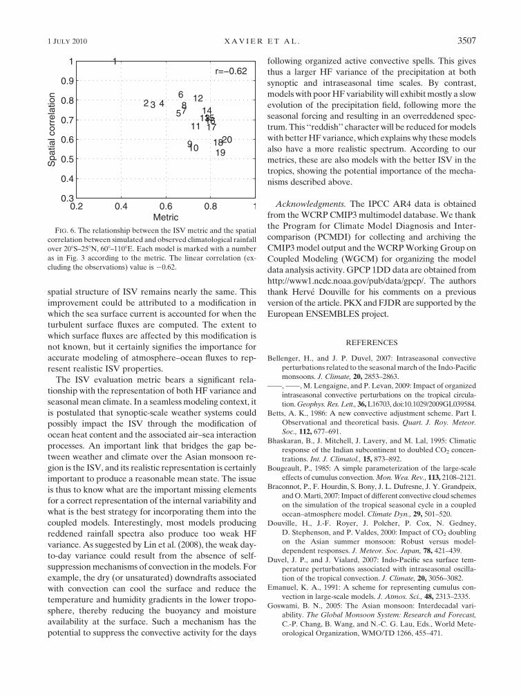
good average rainfall distribution. A correlation of 20.62

(significant at 99% level) suggests a strong tendency for

models with better ISV realism metric to have more spa-

tially consistent monsoon rainfall climatology (Fig. 6). It

is, however, not trivial to establish a direction of cau-

sality for such a link since a correct location of the

convective variability at all time scales (synoptic to in-

traseasonal) is obviously dependent on the correct lo-

cation of the ITCZ. The ISV realism metric implicitly

takes this fact into account since a small distance be-

tween observed and simulated ISV patterns implies a

correct simulation of the main rainfall areas. In such a

case, the ISV realism metric will be mathematically re-

lated to this correlation and hide a possible effect of the

ISV on the representation of the average rainfall dis-

tribution. However, the ISV reproducibility (Fig. 2) is

independent of the observed average rainfall distribu-

tion and can be compared. A link between these two

factors will indicate that the ability of a model to give

reproducible intraseasonal events is somewhat linked to

its ability to give a correct average rainfall distribution.

There is, indeed, a correlation of 20.44 between these

two factors that is significant at the 95% level. This may

also indicate that well-organized and reproducible in-

traseasonal events can develop only in realistic mean

states. The precise knowledge of the origin of this link

needs analyses that are outside the scope of this study.

6. Summary and discussions

Diagnostics on the representation of summer ISV

over the Indian Ocean in the CMIP3 models are pre-

sented with a focus on event-to-event reproducibility

and realism. The LMA used here provides a measure

of the reproducibility and realism by identifying in a

single mathematical form: the perturbation pattern of

each individual organized convective ISV event. This

measure evaluates the robustness of the average ISV

perturbation pattern (Fig. 1). Second, the resemblance

of simulated intraseasonal events to a typical observed

pattern is measured for each simulated ISV event, and

the most probable distance is presented as a metric for

evaluating the simulation of tropical ISV. This gives an

objective evaluation of simulated ISV in terms of their

amplitude, propagation characteristics, and reproduc-

ibility from one event to the other.

The models show a wide range of skills in representing

the ISV. There are a few models that produce realistic

amplitude, propagation characteristics, and event-to-

event reproducibility. Xavier et al. (2008) pointed out

a few issues in representing the intraseasonal air–sea

1 JULY 2010 X A V I E R E T A L . 3505

interaction processes. The lack of representation of di-

urnal SST variability and the associated coupled feed-

backs were proposed to be a source of the DEMETER

model biases. This, however, would require experi-

ments with models that can resolve the oceanic mixed

layer and exchange of fluxes with the atmosphere at

subdiurnal intervals. The convective parameterization is

known to have a strong impact in the climate models

whose signatures can be found even in the deep ocean

circulation (Braconnot et al. 2007). For Atmospheric

Model Intercomparison Project I (AMIP I) simulations,

Slingo et al. (1996) noted that the models with reason-

able levels of intraseasonal activity used convection

schemes with a closure on buoyancy rather than on

moisture supply. Several recent analyses demonstrated

improved MJO simulations for models with mass-flux

convection schemes that use adjustment type of closures

(Liu et al. 2005). However, these findings may be argu-

able since Wang and Schlesinger (1999) demonstrated

that it is possible to alter substantially the strength of the

MJO by modifying the particular trigger used within the

convection scheme as well as the fundamental scheme

itself. The large sensitivity of ISV simulation demands

more dedicated analysis before any conclusions are

drawn on the advantages or drawbacks of any particu-

lar convection scheme. Considering that the large-scale

convective organization depends largely on the con-

vective parameterization, our metric is able to classify

the models based on the convective organization and

thereby highlights the need for improvements in con-

vection schemes. This enhances the utility of the metric

as a diagnostic tool since it can evaluate the drawbacks

in parameterized physics and the complex feedbacks.

One observation is that, as shown in the Table 1, the

BCCR and Centre National de Recherches Meteo-

rologiques (CNRM) models have the same atmospheric

model [Action de Recherche Petite Echelle Grande

Echelle Climate Model (ARPEGE-Climat) Version 3],

and there is a marked improvement in the ISV ampli-

tude in BCCR compared to CNRM, even though the

FIG. 5. (a) Detrended power spectra of JJAS rainfall averaged over 258N–08, 708–1008E in the observations and the

models. (b) The relationship of the ISV metric to the redness of the spectra defined as the ratio of 10–60-day variance

to the 2–10-day variance. (c) The relationship between the metric and total variance in the 2–60-day band. Each

model is marked with a number as in Fig. 3 according to the metric. The linear correlation values (excluding the

observations) in (b) and (c) are indicated.

3506 J O U R N A L O F C L I M A T E VOLUME 23

spatial structure of ISV remains nearly the same. This

improvement could be attributed to a modification in

which the sea surface current is accounted for when the

turbulent surface fluxes are computed. The extent to

which surface fluxes are affected by this modification is

not known, but it certainly signifies the importance for

accurate modeling of atmosphere–ocean fluxes to rep-

resent realistic ISV properties.

The ISV evaluation metric bears a significant rela-

tionship with the representation of both HF variance and

seasonal mean climate. In a seamless modeling context, it

is postulated that synoptic-scale weather systems could

possibly impact the ISV through the modification of

ocean heat content and the associated air–sea interaction

processes. An important link that bridges the gap be-

tween weather and climate over the Asian monsoon re-

gion is the ISV, and its realistic representation is certainly

important to produce a reasonable mean state. The issue

is thus to know what are the important missing elements

for a correct representation of the internal variability and

what is the best strategy for incorporating them into the

coupled models. Interestingly, most models producing

reddened rainfall spectra also produce too weak HF

variance. As suggested by Lin et al. (2008), the weak day-

to-day variance could result from the absence of self-

suppression mechanisms of convection in the models. For

example, the dry (or unsaturated) downdrafts associated

with convection can cool the surface and reduce the

temperature and humidity gradients in the lower tropo-

sphere, thereby reducing the buoyancy and moisture

availability at the surface. Such a mechanism has the

potential to suppress the convective activity for the days

following organized active convective spells. This gives

thus a larger HF variance of the precipitation at both

synoptic and intraseasonal time scales. By contrast,

models with poor HF variability will exhibit mostly a slow

evolution of the precipitation field, following more the

seasonal forcing and resulting in an overreddened spec-

trum. This ‘‘reddish’’ character will be reduced for models

with better HF variance, which explains why these models

also have a more realistic spectrum. According to our

metrics, these are also models with the better ISV in the

tropics, showing the potential importance of the mecha-

nisms described above.

Acknowledgments. The IPCC AR4 data is obtained

from the WCRP CMIP3 multimodel database. We thank

the Program for Climate Model Diagnosis and Inter-

comparison (PCMDI) for collecting and archiving the

CMIP3 model output and the WCRP Working Group on

Coupled Modeling (WGCM) for organizing the model

data analysis activity. GPCP 1DD data are obtained from

http://www1.ncdc.noaa.gov/pub/data/gpcp/. The authors

thank Herve Douville for his comments on a previous

version of the article. PKX and FJDR are supported by the

European ENSEMBLES project.

REFERENCES

Bellenger, H., and J. P. Duvel, 2007: Intraseasonal convective

perturbations related to the seasonal march of the Indo-Pacific

monsoons. J. Climate, 20, 2853–2863.

——, ——, M. Lengaigne, and P. Levan, 2009: Impact of organized

intraseasonal convective perturbations on the tropical circula-

tion. Geophys. Res. Lett., 36, L16703, doi:10.1029/2009GL039584.

Betts, A. K., 1986: A new convective adjustment scheme. Part I.

Observational and theoretical basis. Quart. J. Roy. Meteor.

Soc., 112, 677–691.

Bhaskaran, B., J. Mitchell, J. Lavery, and M. Lal, 1995: Climatic

response of the Indian subcontinent to doubled CO2 concen-

trations. Int. J. Climatol., 15, 873–892.

Bougeault, P., 1985: A simple parameterization of the large-scale

effects of cumulus convection. Mon. Wea. Rev., 113, 2108–2121.

Braconnot, P., F. Hourdin, S. Bony, J. L. Dufresne, J. Y. Grandpeix,

and O. Marti, 2007: Impact of different convective cloud schemes

on the simulation of the tropical seasonal cycle in a coupled

ocean–atmosphere model. Climate Dyn., 29, 501–520.

Douville, H., J.-F. Royer, J. Polcher, P. Cox, N. Gedney,

D. Stephenson, and P. Valdes, 2000: Impact of CO2 doubling

on the Asian summer monsoon: Robust versus model-

dependent responses. J. Meteor. Soc. Japan, 78, 421–439.

Duvel, J. P., and J. Vialard, 2007: Indo-Pacific sea surface tem-

perature perturbations associated with intraseasonal oscilla-

tion of the tropical convection. J. Climate, 20, 3056–3082.

Emanuel, K. A., 1991: A scheme for representing cumulus con-

vection in large-scale models. J. Atmos. Sci., 48, 2313–2335.

Goswami, B. N., 2005: The Asian monsoon: Interdecadal vari-

ability. The Global Monsoon System: Research and Forecast,

C.-P. Chang, B. Wang, and N.-C. G. Lau, Eds., World Mete-

orological Organization, WMO/TD 1266, 455–471.

FIG. 6. The relationship between the ISV metric and the spatial

correlation between simulated and observed climatological rainfall

over 208S–258N, 608–1108E. Each model is marked with a number

as in Fig. 3 according to the metric. The linear correlation (ex-

cluding the observations) value is 20.62.

1 JULY 2010 X A V I E R E T A L . 3507

——, R. S. Ajayamohan, P. K. Xavier, and D. Sengupta, 2003:

Clustering of synoptic activity by Indian summer monsoon

intraseasonal oscillations. Geophys. Res. Lett., 30, 1431,

doi:10.1029/2002GL016734.

——, G. Wu, and T. Yasunari, 2006: Annual cycle, intraseasonal

oscillations and roadblock to seasonal predictability of the

Asian summer monsoon. J. Climate, 19, 5078–5099.

Goulet, L., and J. P. Duvel, 2000: A new approach to detect and

characterize intermittent atmospheric oscillations: Applica-

tion to the intraseasonal oscillation. J. Atmos. Sci., 57, 2397–

2416.

Gregory, D., and P. R. Rowntree, 1990: A mass flux convection

scheme with representation of cloud ensemble characteristics

and stability-dependent closure. Mon. Wea. Rev., 118, 1483–1506.

Huffman, G. J., R. Adler, M. Morrissey, D. Bolvin, S. Curtis,

R. Joyce, B. McGavock, and J. Susskind, 2001: Global pre-

cipitation at one-degree daily resolution from multisatellite

observations. J. Hydrometeor., 2, 36–50.

Kitoh, A., 2006: Asian monsoons in future. The Asian Monsoon,

B. Wang, Ed., Springer/Praxis Publishing, 631–649.

——, S. Yukimoto, A. Noda, and T. Motoi, 1997: Simulated

changes in the Asian summer monsoon at times of increased

atmospheric CO2. J. Meteor. Soc. Japan, 75, 1019–1031.

Lal, M., and S. K. Singh, 2001: Global warming and monsoon cli-

mate. Mausam (New Delhi), 52, 245–262.

Lin, J. L., and Coauthors, 2006: Tropical intraseasonal variability

in 14 IPCC AR4 climate models. Part I: Convective signals.

J. Climate, 19, 2665–2690.

——, K. Weickman, G. Kiladis, B. Mapes, S. Schubert, M. Suarez,

J. Bacmeister, and M. Lee, 2008: Subseasonal variability as-

sociated with Asian summer monsoon simulated by 14 IPCC

AR4 Coupled GCMs. J. Climate, 21, 4541–4567.

Liu, P., B. Wang, K. Sperber, T. Li, and G. Meehl, 2005: MJO in the

NCAR CAM2 with the Tiedtke convective scheme. J. Cli-

mate, 18, 3007–3020.

Madden, R. A., and P. R. Julian, 1994: Observations of the

40–50-day tropical oscillation: A review. Mon. Wea. Rev., 122,813–837.

Meehl, G. A., and W. M. Washington, 1993: South Asian summer

monsoon variability in a model with doubled atmospheric

carbon dioxide concentration. Science, 260, 1101–1104.

——, and J. Arblaster, 2003: Mechanisms for projected future

changes in South Asian monsoon precipitation. Climate Dyn.,

21, 659–675.

Moorthi, S., and M. J. Suarez, 1992: Relaxed Arakawa–Schubert: A

parameterization of moist convection for general circulation

models. Mon. Wea. Rev., 120, 978–1002.

Nordeng, T. E., 1994: Extended versions of the convective pa-

rameterization scheme at ECMWF and their impact on the

mean and transient activity of the model in the tropics.

European Centre for Medium-Range Weather Forecasts,

ECMWF Tech. Memo. 206, 41 pp.

Palmer, T. N., F. Doblas-Reyes, A. Weisheimer, and M. Rodwell,

2008: Toward seamless prediction: Calibration of climate

change projections using seasonal forecasts. Bull. Amer. Me-

teor. Soc., 89, 459–470.

Pan, D.-M., and D. A. Randall, 1998: A cumulus parameterization

with a prognostic closure. Quart. J. Roy. Meteor. Soc., 124,

949–981.

Russell, G. L., J. R. Miller, and D. Rind, 1995: A coupled atmosphere–

ocean model for transient climate change studies. Atmos.–Ocean,

33, 683–730.

Slingo, J. M., and Coauthors, 1996: Intraseasonal oscillations in

15 atmospheric general circulation models: Results from an

AMIP diagnostic subproject. Climate Dyn., 12, 325–357.

Sperber, K. R., and Coauthors, 2001: Dynamical seasonal pre-

dictability of the Asian summer monsoon. Mon. Wea. Rev.,

129, 2226–2248.

Tiedtke, M., 1989: A comprehensive mass flux scheme for cumulus

parameterization in large-scale models. Mon. Wea. Rev., 117,1779–1800.

Waliser, D. E., and Coauthors, 2003: AGCM simulations of in-

traseasonal variability associated with the Asian summer

monsoon. Climate Dyn., 21, 423–446.

Wang, W., and M. E. Schlesinger, 1999: The dependence on con-

vection parameterization of the tropical intraseasonal oscil-

lation simulated by the UIUC 11-layer atmospheric GCM.

J. Climate, 12, 1423–1457.

Wheeler, M., and K. Weickmann, 2001: Real-time monitoring and

prediction of modes of coherent synoptic to intraseasonal

tropical variability. Mon. Wea. Rev., 129, 2677–2694.

——, and H. H. Hendon, 2004: An all-season real-time multivariate

MJO index: Development of an index for monitoring and

prediction. Mon. Wea. Rev., 132, 1917–1932.

Xavier, P. K., J.-P. Duvel, and F. J. Doblas-Reyes, 2008: Boreal

summer intraseasonal variability in coupled seasonal hind-

casts. J. Climate, 21, 4477–4497.

Zhang, G. J., and N. A. McFarlane, 1995: Sensitivity of climate

simulations to the parameterization of cumulus convection

in the Canadian Climate Centre General Circulation Model.

Atmos.–Ocean, 33, 407–446.

Zhao, Z., and W. Kellogg, 1988: Sensitivity of soil moisture to

doubling of carbon dioxide in climate model experiments.

Part II: The Asian monsoon region. J. Climate, 1, 367–378.

3508 J O U R N A L O F C L I M A T E VOLUME 23