TMO Progress Report 42-138 August 15, 1999

An Estimate of Interference Effect From theLos Angeles Area High-Density Fixed

Services (HDFS) on the GoldstoneDSN Receiver Above 30 GHz:

Monte Carlo SimulationC. Ho,1 M. Sue,1 and C. Ruggier1

A large number of microwave transmitters will be installed in large urban centersin the future to provide high-density fixed services (HDFS). The frequency bandproposed for use by these transmitters overlaps the Ka-band (27–40 GHz) allocatedfor NASA’s Deep Space Network (DSN) receivers. Interference signals from thesetransmitters can propagate over the horizon and interfere with the DSN throughvarious mechanisms, such as ducting, rain scattering, and diffraction. In this article,we have used the available International Telecommunication Union (ITU) modelsand a Monte Carlo simulation to estimate the aggregate interference power fromthe HDFS transmitters in the Los Angeles area as received by a DSN station lo-cated at Goldstone, California. It was found that, for a worst-case scenario, whena single transmitter main beam points to the DSN antenna and the separation dis-tance is less than 200 km, the threshold for protecting the DSN receiver at Ka-bandwill be exceeded. An urban area such as Los Angeles has been assumed to have3000 HDFS transmitters spreading with various maximum radial distances. Oursimulation shows that the distributed effective isotropic radiated power (EIRP) ofmultiple HDFS sites will produce higher interference power at Goldstone as com-pared with an equivalent single transmitter with a normally distributed EIRP. Whenthe HDFS spatial distribution has a maximum radial distance of 50 km, the receivedinterference power at Goldstone exceeds the DSN threshold. The aggregate powerand antenna gain increase with increasing transmitter numbers and distributed ra-dial distances. This article provides solid results for consideration by the ITU andthe HDFS community, and presents possible interference-mitigating approaches forthe future HDFS deployment.

I. Introduction

Commercial operators are now proposing to install hundreds and thousands of high-density fixedservices (HDFS) microwave transmitters in large urban centers [1] such as Los Angeles. These trans-mitters will share the same frequencies in the Ka-band (32 GHz and 37 to 38 GHz) with some Space

1 Communication Systems and Research Section.

1

Research Service (SRS) receiving Earth stations. To face this challenge, the World Radio Communi-cations Conference-97 (WRC-97) Resolution 126 requested that the International TelecommunicationUnion–Radio Communication (ITU-R) conduct, as a matter of urgency and in time for the World Ra-dio Communications Conference-99 (WRC-99), appropriate studies to determine sharing criteria betweenstations in the fixed service and stations in other services that are allocated the same frequencies [2].The three DSN worldwide tracking stations utilize this frequency band and may become vulnerable tointerference from the planned deployment of HDFS transmitters. Since these HDFS transmitters operateat relatively strong signal power (up to −60 dBW/Hz), they will seriously interfere with the sensitiveDSN receivers. Thus, it has become imperative to accurately predict the impact of HDFS transmitterson NASA’s DSN receivers in the Ka-band.

The procedures for calculating the coordination distances around an SRS Earth station for interferencefrom a point-to-point transmitter, such as in ITU-R Recommendations IS.847, P.620, and P.452, havebeen well documented [1,3–8]. The procedures in these recommendations are based on the computation ofthe minimum permissible transmission loss that satisfies the protection criteria for emissions originatingat a single station [3–7]. These conditions do not apply to a high-density deployment with multipleterrestrial transmitters over an extended area. Recently, ITU–Joint Rapporteurs Group (ITU-JRG)7D/9D [9–12] developed a method to theoretically calculate the aggregate gain from a large number ofHDFS transmitters by using a normal distribution. They assumed that HDFS transmitter sites will not bespatially distributed, which differs significantly from a real HDFS deployment pattern. Thus, this methodmay underestimate the interference effects, since multiple HDFS transmitters were considered to beequivalent to a single transmitter with an aggregate net power. To simulate a real transmitter distribution,we need to examine the integrated interference power from a large number of HDFS transmitters withvarious spatial distributions. In this article, we followed a Monte Carlo approach to simulate severalthousand HDFS transmitter sites spreading in the Los Angeles area and to calculate the interferencepower received at the Goldstone, California, tracking station. Models and procedures that were used aredescribed in the following section.

II. Models and Procedures

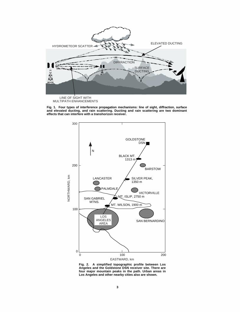
There are several mechanisms [3,5–7,13–15] that can cause the interference signals to propagate withsignificantly low attenuation, as shown in Fig. 1. Other than direct coupling within a line of sight betweenthe receiving Earth station and the transmitter, interference signals also can propagate over the horizonthrough diffraction, surface or elevated ducting, rain scattering, the tropospheric scatter mechanism, etc.[3,5–7]. The diffraction propagation mechanism only makes a contribution at relatively short distances(<200 km) [16], while coupling through rain scattering becomes less effective beyond the 300-km range[17,18]. Ducting-propagation effects, however, remain important over a wider range (∼500 km) [19,20].Interference by tropospheric scatter is generally too low to be considered in this article [13,14].

A. Path Profile Analysis

At first, the profile for the interference-signal propagation path was analyzed to identify which inter-ference mechanisms are related to geomorphologic features [3]. Because the main purpose of this articleis to assess interference effects from transmitters in the Los Angeles area on the Goldstone DSN receiver,a simplified topographic map for this area is presented in Fig. 2. The center of Los Angeles is about200 km away from Goldstone. Along the great circle path between the two locations, there are fourmajor mountain peaks. Two mountain peaks within the San Gabriel Mountains have greater heights(1900 m and 2750 m), which will cause large diffraction losses and partially block the surface-ductingpropagation. However, interference signals still can propagate to the Goldstone site through an elevatedduct and rain scattering. Four small cities behind the San Gabriel Mountains will have lower diffractionlosses since there are no large mountain peaks that block the surface propagation toward the Goldstoneantenna.

2

ELEVATED DUCTINGHYDROMETEOR SCATTER

DIFFRACTION

SURFACEDUCTING

Fig. 1. Four types of interference propagation mechanisms: line of sight, diffraction, surfaceand elevated ducting, and rain scattering. Ducting and rain scattering are two dominanteffects that can interfere with a transhorizon receiver.

LINE OF SIGHT WITHMULTIPATH ENHANCEMENTS

SAN GABRIELMTNS.

MT. WILSON, 1900 m

SILVER PEAK,1350 m

BLACK MT.1313 m

GOLDSTONEDSN

N

LANCASTER

PALMDALEVICTORVILLE

BARSTOW

SAN BERNARDINO

100

200

0100 200

Fig. 2. A simplified topographic profile between LosAngeles and the Goldstone DSN receiver site. There arefour major mountain peaks in the path. Urban areas inLos Angeles and other nearby cities also are shown.

300

MT. ISLIP, 2750 m

EASTWARD, km

NO

RT

HW

AR

D, k

m

0

LOSANGELES

AREA

3

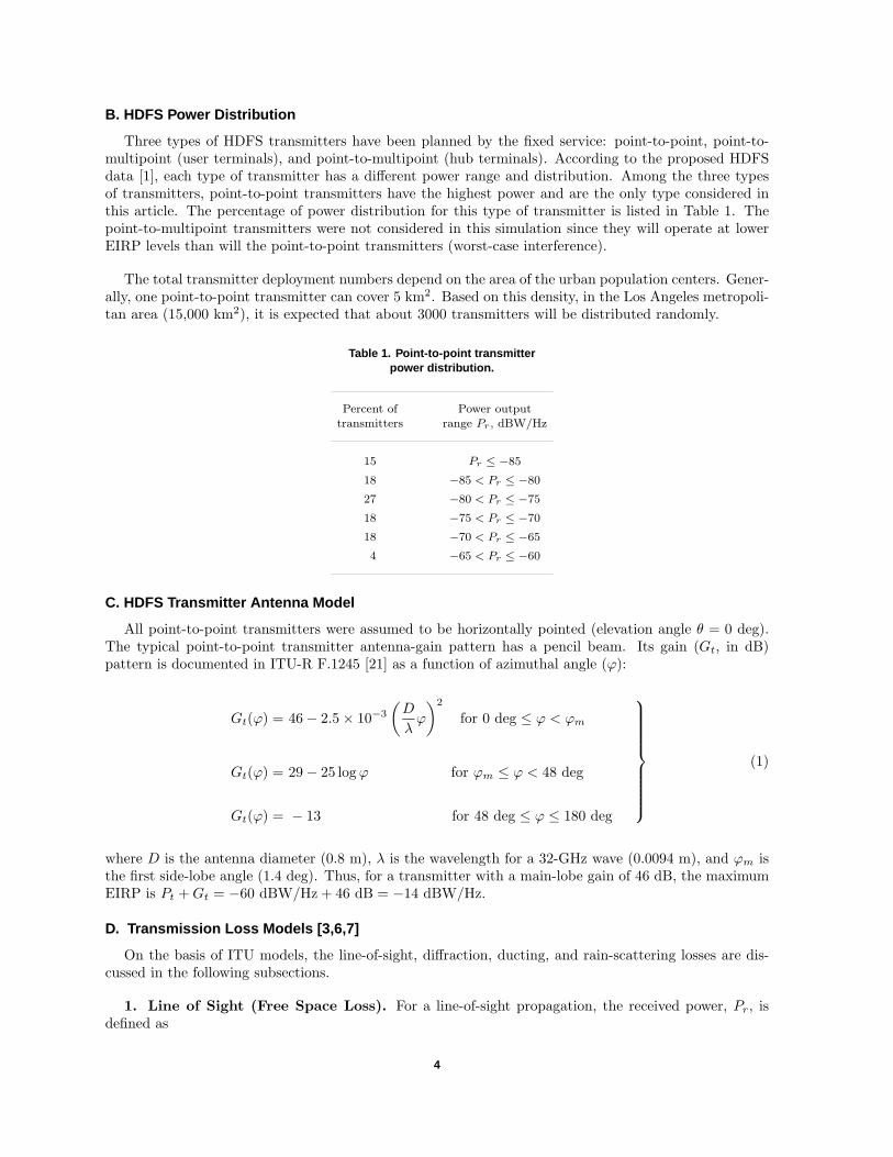
B. HDFS Power Distribution

Three types of HDFS transmitters have been planned by the fixed service: point-to-point, point-to-multipoint (user terminals), and point-to-multipoint (hub terminals). According to the proposed HDFSdata [1], each type of transmitter has a different power range and distribution. Among the three typesof transmitters, point-to-point transmitters have the highest power and are the only type considered inthis article. The percentage of power distribution for this type of transmitter is listed in Table 1. Thepoint-to-multipoint transmitters were not considered in this simulation since they will operate at lowerEIRP levels than will the point-to-point transmitters (worst-case interference).

The total transmitter deployment numbers depend on the area of the urban population centers. Gener-ally, one point-to-point transmitter can cover 5 km2. Based on this density, in the Los Angeles metropoli-tan area (15,000 km2), it is expected that about 3000 transmitters will be distributed randomly.

Table 1. Point-to-point transmitterpower distribution.

Percent of Power outputtransmitters range Pr, dBW/Hz

15 Pr ≤ −85

18 −85 < Pr ≤ −80

27 −80 < Pr ≤ −75

18 −75 < Pr ≤ −70

18 −70 < Pr ≤ −65

4 −65 < Pr ≤ −60

C. HDFS Transmitter Antenna Model

All point-to-point transmitters were assumed to be horizontally pointed (elevation angle θ = 0 deg).The typical point-to-point transmitter antenna-gain pattern has a pencil beam. Its gain (Gt, in dB)pattern is documented in ITU-R F.1245 [21] as a function of azimuthal angle (ϕ):

Gt(ϕ) = 46− 2.5× 10−3

(D

λϕ

)2

for 0 deg ≤ ϕ < ϕm

Gt(ϕ) = 29− 25 logϕ for ϕm ≤ ϕ < 48 deg

Gt(ϕ) = − 13 for 48 deg ≤ ϕ ≤ 180 deg

(1)

where D is the antenna diameter (0.8 m), λ is the wavelength for a 32-GHz wave (0.0094 m), and ϕm isthe first side-lobe angle (1.4 deg). Thus, for a transmitter with a main-lobe gain of 46 dB, the maximumEIRP is Pt +Gt = −60 dBW/Hz + 46 dB = −14 dBW/Hz.

D. Transmission Loss Models [3,6,7]

On the basis of ITU models, the line-of-sight, diffraction, ducting, and rain-scattering losses are dis-cussed in the following subsections.

1. Line of Sight (Free Space Loss). For a line-of-sight propagation, the received power, Pr, isdefined as

4

Pr =PtGtGrLb

=PtGtGrLfsL

(2)

where Lb = LfsL = (PtGtGr)/Pr is the basic transmission loss, Lfs = ([4πdf ]/c)2 is the free space loss,d is the distance between the receiver and transmitter, c is the speed of light, Pt is the transmitter power,and Gr is the receiver antenna gain. Thus, there is a general relation in logarithm:

Pr = EIRP +Gr − Lb (3)

in dB. Furthermore,

Lfs = 20[log(

4πc

)+ log f + log d

](4)

in dB. Changing units of frequency, f , from Hz to GHz, and of d from m to km, we have

Lfs = 92.45 + 20 log f + 20 log d (5)

in dB. In Eq. (2), L is the correction term for loss:

L = Ag +Ad (6)

in dB, where Ag is gaseous attenuation [22], Ad is the defocus factor due to the Earth’s curvature, and

Ag = (γo + γw)d = 0.2d (7)

where γo is loss from oxygen and γw is loss from water vapor, in dB/km. Thus,

Lb − Lfs + L = Lfs +Ag +Ad (8)

in dB. When f = 32 GHz and d = 200 km, we have Lb = 188 dB.

2. Diffraction Over Mountains [16]. Diffraction loss, Ld, is defined as

Ld = Lb + Lds = Lb +∑i

Ji(ν) (9)

in dB, where Lds =∑i Ji(ν) is all subpath diffraction over edges and troughs in the path profiles and

J(ν) is a function defined in [16]. For a 200-km path profile between Los Angeles and Goldstone, thereare four major mountain peaks. The total subpath diffraction loss is

∑i

Ki(ν) = 33

in dB. Thus, total loss due to diffraction is 221 dB over a 200-km path from Los Angeles to Goldstone.

5

3. Transhorizon Ducting (Mode 1) [3,5–7,13,14]. For a transhorizon ducting propagation alongthe great circle of the Earth, the transmission loss, L1, is a function of p, the percentage of time of aweather condition:

L1(p) = 92.5 + 20 log f + 10 log d1 +Ah + [γd(p) + γo + γw]d1 (10)

in dB. Different from a two-dimensional free space loss, 20 log d, given in Eq. (5), ducting propagation hasa one-dimensional loss, 10 log d1, due to tropospheric layer trapment. In Eq. (10), Ah = 7.5 dB is a lossdue to ducting coupling and obstacles, and γd(p) is ducting attenuation (0.1954 dB/km), a function of thepercentage of time. Taking an approximation of 10 log d1 = 20+0.01d1, and γ(p) = 0.01+γd(p)+γo+γw,we have

L1(p) = 120 + 20 log f + γ(p)d1 +Ah (11)

in dB.

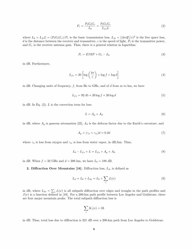
Transmission loss for ducting as a function of required time percentage for which the loss is notexceeded is plotted in Fig. 3 for different distances and for p = 0.001, d1 = 200 km, and γdd1 = 38 dB.Thus,

L1(0.001) = 208

in dB. Corresponding to a larger p, there is a larger loss, L1, or smaller interference. Similarly to Eq. (3),the received interference power is given by

Pr(p) = EIRP +Gr − L1(p) (12)

in dB.

4. Rain Scattering (Mode 2) [3,6,7,17,18,23]. For the rain-scattering transmission loss, L2, adefinition different from that for ducting loss is used. The received interference power is independent ofreceiver antenna gain:

L2(p) =PtPr

(13)

From the radar equation, we have

Pr =PtGrηV Ar

(4π)2(R1)2(R2)2(14)

where η is the cross-section/unit volume, Ar is the effective receiver antenna area, V is the scatteringvolume, and R1 and R2 are distances (km) from rain cells to the transmitter and the receiver, respectively.Transmission loss due to the rain scattering is [6]

L2(p) = 168 + 20 log d2 − 20 log f − 13.2 logR−Gt + 10 logAb − 10 logC + Γ + γgd2 (15)

6

Zone A2 (INLAND) FROM IS.847 MODEL

100 km

200 km

300 km

400 km

500 km

600 km

700 km

800 km

900 km

1000 km

600

500

400

300

200

10-3 10-2 10-1 100

TR

AN

SM

ISS

ION

LO

SS

( L

1 ), d

B

PERCENTAGE OF TIME ( p )

Fig. 3. Transmission loss due to ductingalong a great circle as a function of the per-centage of time in weather exceeded, for dis-tances from 100 to 1000 km.

in dB, where R is the rain rate, a function of percentage of time of the weather condition, Ab, and C andΓ are other correction factors. The loss as a function of p, the percentage of time in weather exceeded, isplotted in Fig. 4 for different distances. For p = 0.001 in rain zone E, a 200-km distance, and a transmittergain of Gt = 46 dB, we have L2 = 160 dB.

Furthermore, we also can represent the loss in another form, because

Pr(p) = Pt − L2(p) = Pt +Gt − L2(p)−Gt

= EIRP − [L2(p) +Gt]

= EIRP − L∗2(p) (16)

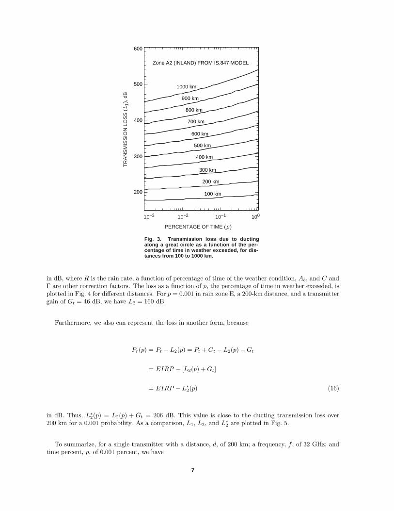
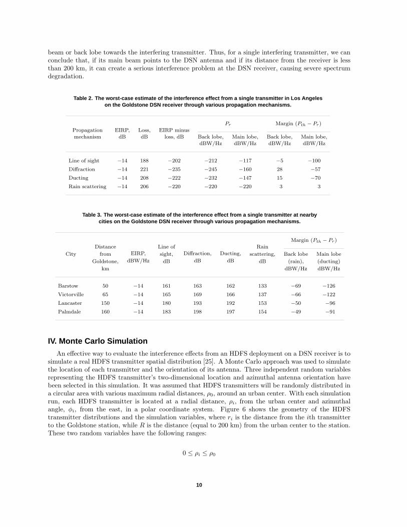
in dB. Thus, L∗2(p) = L2(p) + Gt = 206 dB. This value is close to the ducting transmission loss over200 km for a 0.001 probability. As a comparison, L1, L2, and L∗2 are plotted in Fig. 5.

To summarize, for a single transmitter with a distance, d, of 200 km; a frequency, f , of 32 GHz; andtime percent, p, of 0.001 percent, we have

7

250 km

PROPAGATION MODEL 2(RAIN SCATTERING)

300 km

400 km

500 km

150 km

350 km

450 km

200 km

100 km

250

200

150

100

10-3 10-2 10-1 100

RA

IN S

CA

TT

ER

ING

LO

SS

( L

2 ), d

B

PERCENTAGE OF TIME ( p )

Fig. 4. Transmission loss due to rain scatter-ing as a function of the percentage of time inweather exceeded, for distances from 100 to500 km.

Lb = 188 dB (line-of-sight loss, including gaseous attenuation)

Ld = 221 dB (diffraction loss over mountains)

L1 = 208 dB (ducting transmission loss, 0.001 percent of the time)

L∗2 = 206 dB (rain-scattering loss, 0.001 percent of the time)

Through this comparison, we find that both ducting and rain scattering have smaller transhorizonlosses and, thus, cause stronger coupling of the interference signals. The simulation was performed todetermine interference coupling in the ducting mode only.

5. DSN Receiver Model [24]. There are three NASA DSN receivers, which are located in Gold-stone, California, USA; Canberra, Australia; and Madrid, Spain, respectively. In this article, only theGoldstone 70-m receiver antenna was modeled. DSN operations allow the interference to be exceeded by0.001 percent of the time (weather condition) in order to meet the requirement for manned space missions.This receiver antenna has a gain (pencil-beam) pattern similar to that of a point-to-point transmitterantenna, as described in Subsection II.C [21]. Here we have used a standard large antenna model as doc-umented in ITU Radio Regulations [24] for a DSN antenna pattern with the following parameters: a DSNantenna with a diameter of D = 70 m; a threshold power spectral flux density of pd = −251 dBW/m2Hz atKa-band; and a corresponding threshold power spectral density of Pth = ζπ(D/2)2pd = −217 dBW/Hz,where antenna efficiency, ζ, is 52 percent, main-lobe gain at the bore site is 85 dB, and back-lobe gain is−10 dB.

8

FREE SPACE LOSS

RAIN SCATTERING LOSS ( L2 )

DUCT PROPAGATION LOSS ( L1 )

180

160

140

120

1000 50 100 150

TR

AN

SM

ISS

ION

LO

SS

, dB

i

PROPAGATION DISTANCE, km

Fig. 5. A comparison of transmission lossesdue to ducting and rain scattering as a func-tion of propagation distances for 0.001 per-cent of time in weather exceeded.

200 250 300

200

220

240

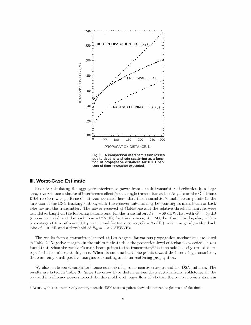
III. Worst-Case Estimate

Prior to calculating the aggregate interference power from a multitransmitter distribution in a largearea, a worst-case estimate of interference effect from a single transmitter at Los Angeles on the GoldstoneDSN receiver was performed. It was assumed here that the transmitter’s main beam points in thedirection of the DSN tracking station, while the receiver antenna may be pointing its main beam or backlobe toward the transmitter. The power received at Goldstone and the relative threshold margins werecalculated based on the following parameters: for the transmitter, Pt = −60 dBW/Hz, with Gt = 46 dB(maximum gain) and the back lobe −12.5 dB; for the distance, d = 200 km from Los Angeles, with apercentage of time of p = 0.001 percent; and for the receiver, Gr = 85 dB (maximum gain), with a backlobe of −10 dB and a threshold of Pth = −217 dBW/Hz.

The results from a transmitter located at Los Angeles for various propagation mechanisms are listedin Table 2. Negative margins in the tables indicate that the protection-level criterion is exceeded. It wasfound that, when the receiver’s main beam points to the transmitter,2 its threshold is easily exceeded ex-cept for in the rain-scattering case. When its antenna back lobe points toward the interfering transmitter,there are only small positive margins for ducting and rain-scattering propagation.

We also made worst-case interference estimates for some nearby cites around the DSN antenna. Theresults are listed in Table 3. Since the cities have distances less than 200 km from Goldstone, all thereceived interference powers exceed the threshold level, regardless of whether the receiver points its main

2 Actually, this situation rarely occurs, since the DSN antenna points above the horizon angles most of the time.

9

beam or back lobe towards the interfering transmitter. Thus, for a single interfering transmitter, we canconclude that, if its main beam points to the DSN antenna and if its distance from the receiver is lessthan 200 km, it can create a serious interference problem at the DSN receiver, causing severe spectrumdegradation.

Table 2. The worst-case estimate of the interference effect from a single transmitter in Los Angeleson the Goldstone DSN receiver through various propagation mechanisms.

Pr Margin (Pth − Pr)Propagation EIRP, Loss, EIRP minusmechanism dB dB loss, dB Back lobe, Main lobe, Back lobe, Main lobe,

dBW/Hz dBW/Hz dBW/Hz dBW/Hz

Line of sight −14 188 −202 −212 −117 −5 −100

Diffraction −14 221 −235 −245 −160 28 −57

Ducting −14 208 −222 −232 −147 15 −70

Rain scattering −14 206 −220 −220 −220 3 3

Table 3. The worst-case estimate of the interference effect from a single transmitter at nearbycities on the Goldstone DSN receiver through various propagation mechanisms.

Margin (Pth − Pr)Distance Line of Rain

EIRP, Diffraction, Ducting,City from sight, scattering, Back lobe Main lobedBW/Hz dB dBGoldstone, dB dB (rain), (ducting)

km dBW/Hz dBW/Hz

Barstow 50 −14 161 163 162 133 −69 −126

Victorville 65 −14 165 169 166 137 −66 −122

Lancaster 150 −14 180 193 192 153 −50 −96

Palmdale 160 −14 183 198 197 154 −49 −91

IV. Monte Carlo Simulation

An effective way to evaluate the interference effects from an HDFS deployment on a DSN receiver is tosimulate a real HDFS transmitter spatial distribution [25]. A Monte Carlo approach was used to simulatethe location of each transmitter and the orientation of its antenna. Three independent random variablesrepresenting the HDFS transmitter’s two-dimensional location and azimuthal antenna orientation havebeen selected in this simulation. It was assumed that HDFS transmitters will be randomly distributed ina circular area with various maximum radial distances, ρ0, around an urban center. With each simulationrun, each HDFS transmitter is located at a radial distance, ρi, from the urban center and azimuthalangle, φi, from the east, in a polar coordinate system. Figure 6 shows the geometry of the HDFStransmitter distributions and the simulation variables, where ri is the distance from the ith transmitterto the Goldstone station, while R is the distance (equal to 200 km) from the urban center to the station.These two random variables have the following ranges:

0 ≤ ρi ≤ ρ0

10

ri

fi

ji

0 xc

HDFS

yc

r0

R

ri

DSN

Fig. 6. HDFS spatial distribution configuration and simulation variables. Transmitters aredeployed in a circular area with a maximum radius, r0

, around the center of Los Angeles.Each transmitter has a random location, (ri , fi ), and a main-beam orientation, ji . The Gold-stone DSN receiver has a distance ri from the receiver and a 200-km distance from the citycenter.

−180 deg ≤ φi ≤ 180 deg

The main beam of the transmitter antenna gain has a fixed elevation angle, θ = 0 deg, and a randomazimuthal angle, ϕ, with

−180 deg ≤ ϕi ≤ 180 deg

Assuming that the Los Angeles metropolitan center has a geographic coordinate (xc, yc), the transmitter’slocation may be described as in a Cartesian coordinate system:

Xi =xi + xc

Yi =yi + yc

(17)

where

xi =ρi cosφi

yi =ρi sinφi

(18)

Considering only the ducting propagation loss, L1, with a time percent of p = 0.001, the total interferencepower spectral flux density, PSFD, can be obtained by non-coherently summing all received powers atGoldstone:

11

PSFD =n∑i

(Pt +Gt(ϕi)− L1(ρi, φi)) (19)

in dB, where the transmitter number is n = 3000 and Pt = −60 dBW/Hz. Each simulation was per-formed with a random HDFS spatial distribution configuration of 3000 transmitters in the Los Angelesarea. Because every transmitter was assigned three random numbers—location, ρi and φi, and antennabeam azimuth orientation, ϕi—9000 independent random numbers were generated for each Monte Carlosimulator run or each HDFS deployment. An interference power value at Goldstone from each patternis obtained by combining the signal from each transmitter as given by Eq. (19). We made 1200 trials(HDFS transmitter spatial distributions), and every trial was initiated with a different sequence of ran-dom numbers. These trials were repeated for different maximum radial distances (ρ0 = 1, 10, 30, and50 km). Finally, 1200 integrated power flux density values were obtained for each fixed HDFS maximumradial distance. Figures 7(a) through 7(c) provide some examples to show the interference power fluxesfor various numbers of transmitters and radial distances.

V. Simulation Results

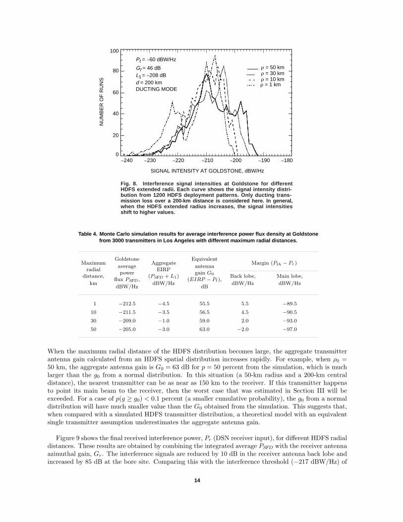
A Monte Carlo approach was used to simulate possible future HDFS transmitter installation patterns.Since a large number of trials were performed, the results for interference power are statistically significant.Figure 8 shows interference PSFD distributions at the Goldstone site for HDFS spatial distributions withdifferent maximum radial distances (1, 10, 30, and 50 km). Each PSFD distribution curve has 1200 sampleswith a 1-dB power increment, as stated in the previous section. The PSFD curves generally shift to higherpower (to the right) with increasing radial distance. Thus, the average power flux also increases with anincreasing radial distance. These PSFD distributions were difficult to model due to large fluctuations inthe curves. However, they are significantly different from a normal (Gaussian) distribution, indicating anonsymmetrical distribution with a gradual tail at the low-power side.

A large number of trials should be performed in a future study to improve the accuracy of the distri-butions. This will lead to determination of the relationship between the aggregate PSFD, the transmitterantenna gain, and the radial distances of HDFS spatial distributions. Some possible HDFS transmitterdeployment patterns with less interference effects on the DSN receiver also can be simulated.

When it is assumed that the aggregate power from multiple HDFS transmitters can be reduced toan equivalent single transmitter, with Pt = −60 dBW/Hz, an equivalent aggregate transmitter antennagain may be deduced. JRG 7D/9D has proposed the use of a theoretical model (normal distribution)for this calculation [9–12]. For a transmitter antenna-gain pattern as described in Subsection II.C [21],m = 46 dB, where m is the mean of the antenna gains averaged over all uniformly distributed azimuthalsamples. For a normal distribution [9, 10], when the probability is p(g ≥ g0) = 50 percent and the totaltransmitter number is n = 3000, the mean aggregate antenna gain for all transmitters is g0 = nm = 55 dB.

In order to make a comparison of the aggregate antenna gain of an equivalent single transmitterdetermined from a normal distribution with an actual HDFS distribution, we also have derived thetransmitter antenna gain from the simulation. Since an actual HDFS transmitter deployment pattern inthe Los Angeles area cannot be known until it is built, an average power flux (the mean values in Fig. 8)is used for the calculation of the aggregate transmitter antenna gain. At first, the aggregate interferencepower spectral flux density, PSFD, at Goldstone as calculated from Eq. (19) is used to infer the equivalentEIRP by (PSFD + L1). For the Los Angeles–Goldstone case, d = 200 km and L1 = 208 dB. Then, usingEIRP−Pt, we can obtain the equivalent aggregate transmitter antenna gain, G0. The results for differentHDFS distribution radial distances are listed in Table 4.

The g0 value determined from the normal distribution was found to approach the equivalent transmit-ter antenna gain, G0 = 55.5 dB, calculated from the simulation, when the radial distance was ρ0 = 1 km.

12

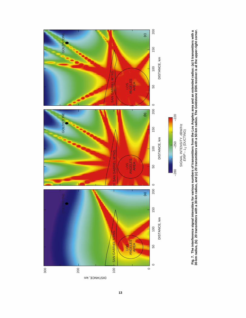
Fig

. 7.

Th

e in

terf

eren

ce s

ign

al in

ten

siti

es f

or

vari

ou

s n

um

ber

s o

f tr

ansm

itte

rs f

rom

th

e L

os

An

gel

es a

rea

and

an

ext

end

ed r

adiu

s: (

a) 5

tra

nsm

itte

rs w

ith

a30

-km

rad

ius,

(b

) 2

0 tr

ansm

itte

rs w

ith

a 3

0-km

rad

ius,

an

d (

c) 2

0 tr

ansm

itte

rs w

ith

a 5

0-km

rad

ius.

Th

e G

old

sto

ne

DS

N r

ecei

ver

is a

t th

e u

pp

er-r

igh

t co

rner

.

(a)

DIS

TA

NC

E, k

m

300

200

100 0

050

100

150

200

DISTANCE, km

-280

-250

-220

SIG

NA

L IN

TE

NS

ITY

, dB

W/H

zE

IRP

- L

1 (D

UC

TIN

G)

(b)

(c)

DIS

TA

NC

E, k

m

050

100

150

200

DIS

TA

NC

E, k

m

050

100

150

200

LOS

AN

GE

LES

AR

EA

LOS

AN

GE

LES

AR

EA

LOS

AN

GE

LES

AR

EA

SA

N G

AB

RIE

L M

TN

S.

SA

N G

AB

RIE

L M

TN

S.

SA

N G

AB

RIE

L M

TN

S.

GO

LDS

TO

NE

GO

LDS

TO

NE

GO

LDS

TO

NE

13

Pt = -60 dBW/Hz

Gt = 46 dBL1 = -208 dBd = 200 kmDUCTING MODE

r = 50 kmr = 30 kmr = 10 km

100

80

60

40

20

0

SIGNAL INTENSITY AT GOLDSTONE, dBW/Hz

-240

NU

MB

ER

OF

RU

NS

-230 -220 -210 -200 -190 -180

Fig. 8. Interference signal intensities at Goldstone for differentHDFS extended radii. Each curve shows the signal intensity distri-bution from 1200 HDFS deployment patterns. Only ducting trans-mission loss over a 200-km distance is considered here. In general,when the HDFS extended radius increases, the signal intensitiesshift to higher values.

r = 1 km

Table 4. Monte Carlo simulation results for average interference power flux density at Goldstonefrom 3000 transmitters in Los Angeles with different maximum radial distances.

Goldstone EquivalentMaximum Aggregate Margin (Pth − Pr)average antenna

radial EIRPpower gain G0distance, (PSFD + L1) Back lobe, Main lobe,

flux PSFD, (EIRP − Pt),km dBW/Hz dBW/Hz dBW/Hz

dBW/Hz dB

1 −212.5 −4.5 55.5 5.5 −89.5

10 −211.5 −3.5 56.5 4.5 −90.5

30 −209.0 −1.0 59.0 2.0 −93.0

50 −205.0 −3.0 63.0 −2.0 −97.0

When the maximum radial distance of the HDFS distribution becomes large, the aggregate transmitterantenna gain calculated from an HDFS spatial distribution increases rapidly. For example, when ρ0 =50 km, the aggregate antenna gain is G0 = 63 dB for p = 50 percent from the simulation, which is muchlarger than the g0 from a normal distribution. In this situation (a 50-km radius and a 200-km centraldistance), the nearest transmitter can be as near as 150 km to the receiver. If this transmitter happensto point its main beam to the receiver, then the worst case that was estimated in Section III will beexceeded. For a case of p(g ≥ g0) < 0.1 percent (a smaller cumulative probability), the g0 from a normaldistribution will have much smaller value than the G0 obtained from the simulation. This suggests that,when compared with a simulated HDFS transmitter distribution, a theoretical model with an equivalentsingle transmitter assumption underestimates the aggregate antenna gain.

Figure 9 shows the final received interference power, Pr (DSN receiver input), for different HDFS radialdistances. These results are obtained by combining the integrated average PSFD with the receiver antennaazimuthal gain, Gr. The interference signals are reduced by 10 dB in the receiver antenna back lobe andincreased by 85 dB at the bore site. Comparing this with the interference threshold (−217 dBW/Hz) of

14

THRESHOLD

-100

-120

-140

-160

-180

-200

ANGLE FROM MAIN BEAM (j)

PO

WE

R R

EC

EIV

ED

(P

r ), d

BW

/Hz

-100 -50 0 50 100 150

Fig. 9. Received interference powers at Goldstone after the DSNreceiver antenna gain in all azimuthal angles. Three curves corre-spond to signals from transmitters with different extended radii. Asa reference, the DSN reciever threshold level also is shown. Whenthe radius is greater than 30 km, the threshold is exceeded.

-150

-220

-240

r = 50 kmr = 30 kmr = 10 kmr =

the DSN receiver, all signals in the main lobe greatly exceed the threshold. In the back-lobe side, whenthe HDFS maximum radial distance is less than 50 km, only small positive margins can be expected.However, if the maximum aggregate PSFD (values in the higher-power side in Fig. 8) are selected witha lower probability, both the aggregate antenna gain and the received power increase by ∼20 dB. Thereceiver’s threshold definitely will be exceeded at all azimuthal angles.

VI. Conclusion and Summary

In this article, an approach was developed to quantitatively estimate, using a Monte Carlo simulation,the aggregate interference power from various transmitter deployment patterns with random orientations.We have estimated the interference level of the HDFS from the Los Angeles area at the Goldstone 70-mDSN tracking station. Based on our results, we find that the HDFS will become a serious problem for theDSN tracking-station receivers, especially when the HDFS transmitter main beams are directly pointedto the DSN antenna. In addition, if HDFS transmitters operate with higher transmitter power or atdistances less than 200 km from the DSN antenna, the receiver’s performance may be severely degraded.We summarize these results in the following.

(1) A thorough literature search was conducted for all ITU documents related to transhori-zon propagation interference effects and all HDFS operating parameters. Interferencefrom a single transmitter through ducting, rain scattering, and diffraction has been fullyinvestigated. Aggregate interference effects from HDFS transmitter spatial distributionshave been assessed using a simulation technique for the first time.

(2) Worst-case estimates were performed for a single transmitter with the highest power levelin the Los Angeles area and the cities near Goldstone. At a 200-km separation distance,when the transmitter’s main beam is exactly pointed at the DSN antenna, only smallpositive margins can be expected relative to the back lobe of the receiver antenna for0.001 percent of the time (weather condition). For some cities with distances less than200 km, interference signals will largely exceed the threshold of the receiver.

15

(3) Monte Carlo simulations were conducted to examine the interference effects on the Gold-stone tracking station using 3000 HDFS transmitters in the Los Angeles area. The impactof HDFS EIRP levels, spatial distributions, and maximum radial distances has been ex-amined. Preliminary statistical results for aggregate power distributions from 1200 trialswith different maximum radial distances of the HDFS distributions were obtained. Theresults show that, when the HDFS transmitter spatial distributions have large radialdistances, aggregate transmitter antenna gains and interference power received at Gold-stone are much greater than those calculated from a normal distribution. When theradial distance is 50 km, the DSN receiver interference threshold will be exceeded.

(4) We have developed an approach, using a Monte Carlo simulation, to quantitatively studythe interference effect of HDFS transmitters with various orientations and distributionson the DSN. As a future study, actual HDFS distributions can be simulated more realis-tically, and any HDFS deployment patterns proposed to mitigate the interference effects,such as coordinated (planned) antenna pointing, can be examined using this simulationtool. This tool also can be used to estimate potential interference to the DSN from othertranshorizon terrestrial services.

Acknowledgments

We would like to thank Dr. Anil V. Kantak for reviewing this article andDr. Nasser Golshan for his suggestions. We also are grateful to Dr. Dan Bathker ofJPL TMOD and to Dr. Louis J. Ippolito of Stanford Telecom ACS for his input.

References

[1] “Elements of a Methodology to Estimate the Global Distribution of PotentialHub Stations of Point-to-Multipoint Fixed Service Systems,” contributed byUSA, Document 7D-9D/36-E, ITU-R, 1998.

[2] “Correspondence Group on High Density Systems in the Fixed Service (HDFS)Above 30 GHz,” Resolutions 126, 726, and 133 (WRC-97), Document 9B/66-E,7D-9D/32, ITU-R, 1998.

[3] “Prediction Procedure for the Evaluation of Microwave Interference BetweenStations on the Surface of the Earth at Frequencies Above About 0.7 GHz,”Recommendation ITU-R P.452-8, ITU-R, 1997.

[4] “Method for the Determination of the Coordination Area Around an Earth Sta-tion in Frequency Band Between 1 GHz and 40 GHz Shared Between Space andTerrestrial Radio Communication Services,” Appendix S7 (28), Radio Regula-tions, ITU-R, 1994.

[5] “A Comparison of Coordination Distances for Propagation Mode (1) of Ap-pendix S7 Calculated Using Recommendation ITU-R P.620-3 and Recommen-dation ITU-R IS.847-1, and Data Measured in Europe for Frequencies Between6 and 30 GHz,” contributed by UK, Document 3M/25-E, ITU-R, 1998.

16

[6] “Determination of the Coordination Area of an Earth Station Operating With aGeostationary Space Station and Using the Same Frequency Band as a Systemin a Terrestrial Service,” Recommendation ITU-R IS.847-1, ITU-R, 1993.

[7] “Propagation Data Required for the Evaluation of Coordination Distances in theFrequency Range 0.85–60 GHz,” Recommendation ITU-R P.620-3, ITU-R, 1997.

[8] CCIR, “Propagation Data Required for the Evaluation of Coordination Distancein the Frequency Range 1–40 GHz,” Report 724-2, in vol. V, Propagation in Non-Ionized Media, Recommendations and Reports of the CCIR, 1986, Geneva: Intl.Telecomm. Union, 1986.

[9] “Consideration of the Statistical Characteristics of Parameters Affecting SharingBetween Stations in the Space Research Service and HDFS Stations in the FixedService in Bands Above 30 GHz,” contributed by USA, Document US7D-9D/xxx,ITU-R, 1998.

[10] “Methodology to Estimate the Number of Stations and to Aggregate the Emis-sions of High-Density Fixed Systems in the Fixed Service for the Purpose of De-termining the Coordination Contour and Coordination Distance in Bands Above30 GHz Shared with Receiving Earth Stations in the Space Research Service,”contributed by USA, Document USJRG 7D-9D/xyz, ITU-R, 1999.

[11] “Co-Frequency Sharing of Spectrum Between High-Density Fixed Systems andSpace Research Systems in the 31.8–32.3 GHz Band,” contributed by Canada,Document 7D-9D/31-E, ITU-R, 1998.

[12] “Co-Frequency Sharing of Spectrum Between High-Density Fixed Systems andScientific Satellite Systems in the 37–38 GHz and 40.0–40.5 GHz Bands,” con-tributed by Canada, Document 7D-9D/39-E, ITU-R, 1998.

[13] CCIR, “Radiometeorological Data,” Report 563-3, in vol. V, Propagation in Non-Ionized Media, Recommendations and Reports of the CCIR, 1986, Geneva: Intl.Telecomm. Union, 1986.

[14] CCIR, “Effects of Tropospheric Refraction on Radiowave Propagation,” Report718-2, in vol. V, Propagation in Non-Ionized Media, Recommendations and Re-ports of the CCIR, 1886, Geneva: Intl. Telecomm. Union, 1986.

[15] B. R. Bean and E. J. Dutton, Radio Meteorology, New York: Dover PublicationsInc., 1966.

[16] “Propagation by Diffraction,” Recommendation ITU-R P.526-5, ITU-R, 1997.

[17] R. K. Crane, “Bistatic Scatter From Rain,” IEEE Trans. Ant. Prop., vol. AP-22,pp. 312–320, 1974.

[18] J. Awaka, K. Nakamura, and H. Inomata, “Bistatic Rain-Scatter Experiment at34.8 GHz,” IEEE Trans. Ant. Prop., vol. AP-31, pp. 693–698, 1983.

[19] M. P. M. Hall, editor, Effects of the Troposphere on Radio Communication, Lon-don: Peter Peregrinus, 1980.

[20] R. K. Crane, “A Review of Transhorizon Propagation Phenomena,” Radio Sci.,vol. 16, pp. 649–669, 1981.

[21] “Mathematical Model of Average Radiation Patterns for Line-of-Sight Point-to-Point Radio-Relay System Antennas for Use in Certain Coordination Studiesand Interference Assessment in the Frequency Range From 1 to About 40 GHz,”Recommendation ITU-R F.1245, ITU-R, 1997.

17

[22] CCIR, “Attenuation by Atmospheric Gases,” Report 719-2, in vol. V, Propaga-tion in Non-Ionized Media, Recommendations and Reports of the CCIR, 1886,Geneva: Intl. Telecomm. Union, 1986.

[23] CCIR, “Scattering by Precipitation,” Report 882-1, in vol. V, Propagation inNon-Ionized Media, Recommendations and Reports of the CCIR, 1886, Geneva:Intl. Telecomm. Union, 1986.

[24] Radio Regulations 3, Appendices 25–44, Norwegian Telecommunications Admin-istration, Oslo, 1982.

[25] “Principles and a Methodology for Frequency Sharing in the 1610.6–1613.8 and1660–1660.5 MHz Bands Between the Mobile-Satellite Service (Earth-to-Space)and the Radio Astronomy Service,” contributed by Radiocommunication StudyGroup 8, Document 8/1021-E, ITU-R M., ITU-R, 1997.

18