Embed Size (px)
Citation preview

An Energy-Regenerative Vehicle Suspension
System – Development, Optimization, and
Improvement
by
Bo Huang
M.Phil., The Hong Kong University of Science and Technology, 2010
B.Eng., Tianjin University, 2007
Thesis Submitted in Partial Fulfillment of the
Requirements for the Degree of
Doctor of Philosophy
in the
School of Mechatronic Systems Engineering
Faculty of Applied Sciences
Bo Huang 2016
SIMON FRASER UNIVERSITY
Summer 2016

ii
Approval
Name: Bo Huang
Degree: Doctor of Philosophy
Title of Thesis: An Energy-Regenerative Vehicle Suspension System – Development, Optimization, and Improvement
Examining Committee: Chair: Amr Marzouk Lecturer
Farid Golnaraghi Senior Supervisor Professor
Mehrdad Moallem Supervisor Professor
Siamak Arzanpour Supervisor Associate Professor
Gary Wang Internal Examiner Professor School of Mechatronic Systems Engineering
Ebrahim Esmailzadeh External Examiner Professor Department of Automotive, Mechanical and Manufacturing Engineering University of Ontario Institute of Technology
Date Defended/Approved:
August 23, 2016

iii
Abstract
With the rapid development of hybrid and fully electric vehicles,
electromagnetic suspensions have shown great potential for capturing energy
while offering high-level ride comfort. The objective of this research was to
develop an electromagnetic-based vehicle suspension system that allows for
regeneration of road-induced vibration energy and supplies better dynamics
control. A small-scale proof-of-concept system consisting of a mass-spring-
damper system, ball screw mechanism, and direct current (DC) machine was
designed. The vibration energy in the mass-spring-damper system caused
vertical motion of sprung mass and the ball screw mechanism to convert the
translational motion into rotary motion, which resulted in the generation of back
electromotive force of the DC machine.
Systematic optimization methodologies were utilized to provide for
selective adaption of suspension parameters, such as spring constant (rate) and
damping coefficient, according to different road surface conditions, including
harmonic and stochastic waveforms. By maximizing the average of power
generation or minimizing the root-mean-square of the sprung mass’s absolute
acceleration by selecting optimal parameters, the suspension allowed operation
in either energy-oriented mode or control-oriented mode.
Furthermore, a bandwidth enhancement technique utilizing cubic
nonlinearities was demonstrated to improve the energy harvesting capability of
the suspension system. A self-powered regenerative Skyhook control strategy
was proposed to overcome the trade-off between passive control (insufficient
control) and active control (external energy demand) for the suspension system.
Keywords: Energy harvesting, regenerative vehicle suspension, design optimization, bandwidth enhancement, Skyhook control

iv
Dedication
To my beloved wife, Xueling, and my daughter, Lydia
To my parents

v
Acknowledgements
It is my pleasure to express my deep gratitude to my senior supervisor, Dr.
Farid Golnaraghi, for his tremendous support and patient guidance during my
Ph.D. study. His experience and insight into this research are invaluable, and
have helped me advance and achieve my academic goals.
Moreover, I would like to thank my co-supervisor, Dr. Mehrdad Moallem,
and my supervisory committee member, Dr. Siamak Arzanpour, for taking their
time and effort and providing valuable advices through my research. I would also
like to thank my internal and external examiners, Dr. Gary Wang and Dr. Ebrahim
Esmailzadeh, for attending my Ph.D. defence and giving helpful feedback on this
thesis. In addition, I would like to thank my friends and colleagues, Dr. Chen-Yu
Hsieh and Dr. Amr Marzouk, for their collaboration and help in working on this
project.
Finally, it does not matter where I am, it matters who I am with that makes
life meaningful. I would like to give special thanks to my wife and my parents, for
their love that becomes the most important support and encouragement for every
progress I have made.

vi
Table of Contents
Approval ................................................................................................................ ii Abstract ................................................................................................................ iii Dedication ............................................................................................................ iv Acknowledgements ............................................................................................... v
Table of Contents ................................................................................................. vi List of Tables ....................................................................................................... ix List of Figures ....................................................................................................... x
List of Acronyms ................................................................................................. xv Nomenclature .....................................................................................................xvi
Chapter 1. Introduction ...................................................................................... 1
1.1. Traditional Vehicle Suspension Systems ...................................................... 3 1.1.1. Passive Suspension Systems ............................................................ 5 1.1.2. Semi-Active Suspension Systems ...................................................... 6
1.1.3. Active Suspension Systems ............................................................... 7 1.2. Energy-Regenerative Suspension Systems ................................................. 7
1.3. Optimal Design of Suspension Systems ..................................................... 11 1.4. Bandwidth Enhancement ............................................................................ 14
1.5. Research Objectives and Thesis Outline .................................................... 16 1.6. Thesis Contributions ................................................................................... 18
Chapter 2. Development of an Energy-Regenerative Suspension System ............................................................................................ 19
2.1. System Description and Prototype Design ................................................. 19
2.2. Mathematical Modeling ............................................................................... 21
2.2.1. DC Motor and Generator .................................................................. 21 2.2.2. Ball Screw Mechanism ..................................................................... 23 2.2.3. Output Force of the Regenerative Damper ...................................... 24
2.2.4. Dynamics of the Quarter-Car Suspension System ........................... 25 2.3. Numerical Simulation and Experimental Test ............................................. 26
2.3.1. Equivalent Damping Ratio ................................................................ 28 2.3.2. Time Responses Based on Harmonic Excitations ............................ 30 2.3.3. Frequency Responses Based on Harmonic Excitations ................... 32
2.3.4. Power Regeneration Efficiency ........................................................ 33 2.4. Conclusion .................................................................................................. 37
Chapter 3. Optimization of Energy-Regenerative Suspension System Under Harmonic Excitation ........................................................... 38
3.1. System Performance Indices ...................................................................... 38

vii
3.1.1. Ride Comfort – Absolute Acceleration Transmissibility .................... 38 3.1.2. Energy Harvesting – Power Generation Transmissibility ................. 39
3.2. Problem Definition ...................................................................................... 42 3.3. Optimization Procedure .............................................................................. 43
3.3.1. Flowchart of the Optimization Procedure ......................................... 43 3.3.2. Optimization Design Chart ............................................................... 45 3.3.3. Global Optimization .......................................................................... 46
3.3.4. Local Optimization ............................................................................ 46 3.4. Simulation and Experimental Results ......................................................... 49
3.5. Conclusion .................................................................................................. 51
Chapter 4. Optimization of Energy-Regenerative Suspension System Under Stochastic Road Excitation................................................ 52
4.1. Problem Definition ...................................................................................... 52
4.1.1. Alternative Dynamic Equations of the Suspension System .............. 52 4.1.2. Standard Road Profile ...................................................................... 54
4.1.3. Ground-Tire Interface ....................................................................... 54 4.1.4. The Ride Comfort Cost Function ...................................................... 55
4.1.5. The Power Generation Cost Function .............................................. 58 4.2. Optimization Procedure .............................................................................. 60
4.2.1. Optimization Rule and Design Chart ................................................ 61
4.2.2. Local Optimization for Energy Harvesting ........................................ 63 4.3. Simulation and Experimental Results ......................................................... 66
4.3.1. Road Profile Generation ................................................................... 66 4.3.2. System Performance of Ride Comfort and Power Generation ......... 67
4.4. Conclusion .................................................................................................. 73
Chapter 5. Bandwidth Enhancement Utilizing Nonlinear Stiffness .............. 74
5.1. Motivation ................................................................................................... 74
5.2. Nonlinear Variable Inductor System ........................................................... 77 5.2.1. System Description and Modeling .................................................... 77
5.2.2. Theoretical Analysis ......................................................................... 80 5.3. Physical Nonlinear Spring System Versus Synthesized Nonlinear
Inductor System .......................................................................................... 91 5.4. Piecewise Linear Spring System ................................................................ 96
5.4.1. Introduction ...................................................................................... 96
5.4.2. System Description and Modeling .................................................... 98 5.4.3. Perturbation Analysis ..................................................................... 101
5.4.4. Power Generation and Bandwidth Analysis ................................... 108 5.4.5. Experimental Setup and Test Results ............................................ 111
5.5. Conclusion ................................................................................................ 120

viii
Chapter 6. Regenerative Skyhook Control for the Hybrid Vehicle Suspension System ..................................................................... 122
6.1. Control Methods for Vehicle Suspension Systems ................................... 122 6.1.1. Active Skyhook Control .................................................................. 123 6.1.2. Semi-Active Skyhook Control ......................................................... 124 6.1.3. Semi-Active Rakheja-Sankar Control ............................................. 126 6.1.4. Modified Skyhook Control .............................................................. 126
6.1.5. Comparison of Different Control Methods ...................................... 128 6.2. Operation Modes for the Hybrid Suspension System ............................... 132
6.2.1. Schematic of the Hybrid Suspension System................................. 132 6.2.2. Conditions of Self-Powered Control ............................................... 133
6.3. Numerical Simulation Results ................................................................... 136 6.4. Conclusion ................................................................................................ 138
Chapter 7. Conclusion and Future Work ...................................................... 140 7.1. Conclusion ................................................................................................ 140
7.2. Future Work .............................................................................................. 142
References ...................................................................................................... 144

ix
List of Tables
Table 2.1 Parameter values of the experimental setup ....................................... 28
Table 2.2 Values of load resistor and equivalent damping ratio .......................... 30
Table 3.1 Experimental results of performance indices for different load resistances .................................................................................... 51
Table 4.1 Different driving situations ................................................................... 62
Table 4.2 Experimental results of performance indices in Highway I and City situations ................................................................................ 73
Table 5.1 Equivalent parameters of the nonlinear suspension model ................. 80
Table 5.2 Comparison of FoMs for linear and nonlinear energy harvesters ...... 116

x
List of Figures
Figure 1.1 Mercedes-Benz active suspension system .......................................... 2
Figure 1.2 2-DOF quarter-car suspension model .................................................. 4
Figure 1.3 1-DOF linear model of suspension systems: (a) passive suspension, (b) semi-active suspension, and (c) active suspension ...................................................................................... 5
Figure 1.4 Electromagnetic (EM) damper using ball screw and nut ...................... 9
Figure 1.5 Schematic view of a hybrid EM damper ............................................. 10
Figure 1.6 EM shock absorber using a rack-pinion mechanism .......................... 10
Figure 1.7 EM suspension using an algebraic screw mechanism ....................... 10
Figure 1.8 Root-mean-square (RMS) optimization design chart ......................... 14
Figure 2.1 1-DOF model of the regenerative suspension system ....................... 20
Figure 2.2 CAD prototype of the regenerative suspension system ..................... 20
Figure 2.3 Circuit diagram of motor/generator .................................................... 21
Figure 2.4 Dynamics of ball screw and DC motor ............................................... 24
Figure 2.5 Experimental test setup for the regenerative suspension system ...... 27
Figure 2.6 Damping ratios with different load resistances ................................... 30
Figure 2.7 Time responses based on harmonic excitations in (a) 5 Hz and (b) 8 Hz .......................................................................................... 31
Figure 2.8 Frequency responses of relative displacement, absolute acceleration and generated power from experimental results (a-c) and simulation results (d-f) .................................................... 33
Figure 2.9 Mechanical efficiency of the system with 30 Ω load resistance for different excitation frequencies ................................................. 34
Figure 2.10 Electrical efficiency of the system with 30 Ω load resistance for different excitation frequencies ................................................. 36
Figure 2.11 Power regeneration efficiency of the system ................................... 36

xi
Figure 3.1 Flowchart of the optimization procedure ............................................ 44
Figure 3.2 Contour curves for functions and
in terms of ( ),
and optimization points for ride comfort and power generation ..................................................................................... 46
Figure 3.3 Local optimization for ride comfort performance versus damping coefficient for various spring constants ........................... 48
Figure 3.4 Local optimization for power generation performance versus damping coefficient for various spring constants ........................... 48
Figure 3.5 RMS of absolute acceleration transmissibility versus damping coefficient ...................................................................................... 50
Figure 3.6 Average of power generation transmissibility versus damping coefficient ...................................................................................... 50
Figure 4.1 Contour curves for functions and in terms of ( ) and optimum points for ride comfort and power generation, based on different driving situations: (a) Highway I, (b) Highway II, (c) City, and (d) Off-road ............................................. 62
Figure 4.2 Local optimization for energy harvesting in a City driving
situation when the spring constant is selected as , respectively ................................................................................... 66
Figure 4.3 Standard road profile for (a) Highway I and (b) City situations ........... 67
Figure 4.4 Power spectral density of road profile for (a) Highway I and (b) City situations ................................................................................ 67
Figure 4.5 Comparison of RMS of absolute acceleration between analytical solution and experimental test for (a) Highway I situation and soft spring setup, (b) Highway I situation and hard spring setup, (c) City situation and soft spring setup, and (d) City situation and hard spring setup .................................. 69
Figure 4.6 Comparison of expectation of generated power between analytical solution and experimental test for (a) Highway I situation and soft spring setup, (b) Highway I situation and hard spring setup, (c) City situation and soft spring setup, and (d) City situation and hard spring setup .................................. 70

xii
Figure 4.7 System responses in the Highway I situation with optimal damping for best ride comfort performance: (a) absolute acceleration and (b) generated power; for best power generation performance: (c) absolute acceleration and (d) generated power ........................................................................... 71
Figure 4.8 System responses in the City situation with optimal damping for best ride comfort performance: (a) absolute acceleration and (b) generated power; for best power generation performance: (c) absolute acceleration and (d) generated power ....................... 72
Figure 5.1 A simple model of a linear suspension system and its frequency-response curve ............................................................. 75
Figure 5.2 Frequency-response curves of linear and nonlinear systems ............ 76
Figure 5.3 1-DOF model of the regenerative suspension system with (a) physical nonlinear spring and (b) nonlinear variable inductor ........ 77
Figure 5.4 Frequency responses of the system at primary resonance: (a) amplitude curve and (b) phase curve ............................................ 88
Figure 5.5 State plane of ( ) for , where two stable solutions exist ....... 89
Figure 5.6 Jump phenomena of the system at primary resonance: (a) amplitude curve and (b) phase curve ............................................ 90
Figure 5.7 Time responses of the system at primary resonance: (a) low
frequency ( ) and (b) high frequency ( ) ....................... 91
Figure 5.8 Lord controlled equilibrium mount system .......................................... 96
Figure 5.9 1-DOF piecewise linear oscillator and its stiffness property ............... 97
Figure 5.10 Cubic curve and piecewise linear fitting curve ................................. 98
Figure 5.11 Mechanical model of the nonlinear regenerative suspension system ........................................................................................... 99
Figure 5.12 Stiffness of the system in terms of the relative displacement ........... 99
Figure 5.13 The analytical frequency-response curves of the relative displacement: (a) amplitude and (b) phase ................................. 107
Figure 5.14 Jump phenomena of relative displacement curves: (a) amplitude and (b) phase .............................................................. 108

xiii
Figure 5.15 Frequency-response curve of power generation and bandwidth .................................................................................... 109
Figure 5.16 CAD prototype of the regenerative suspension system with piecewise springs ........................................................................ 112
Figure 5.17 Experimental test setup for the regenerative suspension system with piecewise springs .................................................... 112
Figure 5.18 Experimental frequency responses of the regenerative suspension system with piecewise springs: (a) relative displacement and (b) generated power ....................................... 114
Figure 5.19 Comparison between linear and nonlinear systems ...................... 115
Figure 5.20 Mechanical, electrical, and overall efficiency of power generation ................................................................................... 116
Figure 5.21 FoM for different values of load resistor ......................................... 117
Figure 5.22 FoM for different values of coupler clearance ................................ 117
Figure 5.23 Stochastic road profile to simulate a City situation ......................... 118
Figure 5.24 Relative displacement of linear and nonlinear systems ................. 119
Figure 5.25 Absolute acceleration of linear and nonlinear systems .................. 119
Figure 5.26 Generated power of of linear and nonlinear systems ..................... 120
Figure 6.1 Schematic structure of a typical Skyhook control system model ...... 123
Figure 6.2 Situation of a vehicle running through a speed hump ...................... 129
Figure 6.3 Profile of the bump excitation ........................................................... 129
Figure 6.4 Absolute acceleration responses of the system with different control methods based on bump excitation ................................. 130
Figure 6.5 Absolute acceleration responses of the system with different control methods based on harmonic excitation ........................... 131
Figure 6.6 RMS of absolute acceleration transmissibility for different control methods ........................................................................... 132
Figure 6.7 Schematic of the hybrid suspension system .................................... 133

xiv
Figure 6.8 Algorithm for determining the suspension system operating with the self-powered regenerative Skyhook control strategy ............. 135
Figure 6.9 Excitation profile with frequency sweeping from 2 Hz to 9 Hz .......... 136
Figure 6.10 Absolute acceleration of the sprung mass for passive and controlled systems: (a) 0 - 7 s and (b) zoomed-in at 1 s - 3 s ...... 137
Figure 6.11 Instantaneous power and cumulative energy of the battery ........... 138

xv
List of Acronyms
back-EMF Back electromotive force
cc Complex conjugate
DC Direct current
EM Electromagnetic
EVs Electrical vehicles
GVs Gasoline vehicles
MSE Mean-square error
MR Magneto-rheological
PSD Power spectral density
RMS Root-mean-square
SMR Switch-mode rectifier
1-DOF One-degree-of-freedom
2-DOF Two-degrees-of-freedom

xvi
Nomenclature
Symbol Description Unit Symbol Description Unit
Absolute acceleration transmissibility of the sprung mass
1/s2 Average of power generation transmissibility
W/m2
Normalized value of
1 Motor damping
coefficient N·s/m
Viscous damping coefficient
N·s/m Upper bound of the damping coefficient
N·s/m
Lower bound of the damping coefficient
N·s/m Optimal damping coefficient
N·s/m
Semi-active damping coefficient
N·s/m Damping coefficient of the Skyhook damper
N·s/m
Coefficient of the ball screw
mm/rad Total energy into the system
J
Energy absorbed by the DC motor/generator
J Required energy for the damping force
J
Energy dissipated by viscous damping
J Cumulative generated energy
J
Kinetic and potential energies
J Back-EMF voltage V
Expectation of generated power by the damper
W Temporal excitation frequency
Hz
Output force of the shock absorber
N Temporal cut-off frequency of the filter to simulate ground-tire interface
Hz
Full cut-off temporal frequency
Hz Natural frequency Hz
Road displacement PSD
m3 Road roughness coefficient
m3

xvii
Current through the load resistor
A Instantaneous current through the inductor
A
Reference current of SMR
A Inertia of the ball screw
kg·m2
Inertia of the gearbox
kg·m2 Inertia of the motor kg·m2
Spring constant N/m First spring constant of the piecewise spring system
N/m
Second spring constant of the piecewise spring system
N/m Back-EMF coefficient
V/rad/s
Transmission ratio of the gearbox
1 Nonlinear stiffness N/m
Torque constant N·m/A Lead ratio of the ball screw
mm/rev
Inductance in SMR H Nonlinear inductance
H
Sprung mass kg Spatial frequency
( )
m-1
Reference spatial
frequency ( )
m-1 Full cut-off spatial frequency
m-1
Power generation transmissibility
W/m2 Average power flow per cycle
W
Desired power for the damping force
W Instantaneous power generated by the damper
W
Internal resistance of DC motor
Ω Load resistance Ω
RMS of absolute acceleration transmissibility
1/s2 Normalized value of
1
PSD of absolute acceleration of the sprung mass
m2/ s3·rad
PSD of relative velocity between sprung mass and excitation
m2/ s·rad

xviii
Relative velocity transmissibility
1/s Vehicle speed m/s
Terminal voltage controlled by SMR
V Terminal voltage of the load resistor
V
Road index (=2) 1 Length of the tire footprint
m
Displacement of the sprung mass
m Velocity of the sprung mass
m/s
Acceleration of the sprung mass
m/s2 Displacement of base excitation
m
Velocity of base excitation
m/s Acceleration of base excitation
m/s2
Stroke displacement of the shock absorber
m Stroke velocity of the shock absorber
m/s
Stroke acceleration of the shock absorber
m/s2 Factor of the nonlinearity
1
Clearance of the coupler
mm Damping ratio 1
Total efficiency of power regeneration
1 Efficiency of the ball screw
1
Electrical efficiency of power transfer
1 Efficiency of the gearbox
1
DC generator efficiency
1 Mechanical efficiency of energy generation
1
SMR power conversion efficiency
1 Angular displacement of the motor gear shaft
rad
Angular velocity of the motor gear shaft
rad/s Angular acceleration of the motor gear shaft
rad/s2
Relative displacement transmissibility
1 Detuning parameter for the nearness of excitation frequency to natural frequency
1

xix
Output torque of the shock absorber
N·m Output torque of the motor
N·m
Flux of the inductor V·s Excitation frequency rad/s
Radian cut-off frequency of the filter to simulate ground-tire interface
rad/s Natural frequency rad/s

1
Chapter 1. Introduction
Today, conventional gasoline vehicles (GVs) still have the edge in the
market. However, partly due to their exhaust gas, air pollution is becoming more
serious. Electric vehicles (EVs) are consequently becoming more popular. This
has to do with their numerous attractive properties, which are listed below (U.S.
Department of Energy, n.d.):
- They are environmentally friendly. EVs help improve the green environment since they emit no exhaust gas pollutants. Also, electricity can be generated from clean energy produced at nuclear-, solar-, or wind-powered plants. Such energy causes no air pollution.
- They are characterized by performance improvements. Electric motors used in EVs offer quieter operation, faster responses, and stronger acceleration than most GVs.
- They cost less. The price of electricity is only about one sixth of that of gas. Moreover, EVs require less maintenance than GVs.
- They are energy efficient. EVs convert about 59-62% of energy from the grid to power their wheels. This is about three times higher than what GVs convert.
With the development of EVs, extending the range of battery power has
become increasingly important. This will help overcome the significant battery-
related challenges of EVs, for instance, their limited driving ranges and long
recharge times. A new approach to increasing the battery range is the use of
energy-harvesting technology in vehicle parts such as the suspension system
(Hsu, 1996).

2
Figure 1.1 illustrates a typical suspension system in Mercedes-Benz S-
Class vehicles (Mercedes-Benz: Magic Body Control, n.d.). An automotive
suspension system supports the vehicle body on the axles and suppresses
undesirable vibration from road roughness. It is responsible for enhancing
passengers’ ride comfort and vehicles’ road handling characteristics by
absorbing the induced energy from the road into a spring and dissipating it into
heat over time using a damper. Traditional suspension systems, such as passive
suspension systems, have conventional springs and oil dampers with constant
properties that are inexpensive and simple to manufacture, but performance is
limited due to their compromise between ride comfort and road handling. To
achieve better vibration isolation and control performance, many semi-active and
active suspension systems have been designed (Dyer, 2015). However, these
sophisticated systems need additional power to realize control tasks. To this end,
sufficient available power is of the greatest importance. In addition, range of
battery power has been introduced as a new performance indicator for EVs and
hybrid EVs.
Figure 1.1 Mercedes-Benz active suspension system
Recent attention to vibration-based energy harvesting has resulted in the
creation of techniques for regenerative vehicle suspension. Rather than

3
dissipating energy through viscous damping, the suspension is able to convert
the mechanical energy from systems into electrical energy and charge the
battery directly. Therefore, a self-powered suspension system has been taken
into consideration. The system is able to produce control force using regenerated
power from the damper with no additional energy cost. Furthermore, the
remaining energy can be used to extend the power range which is a strong merit
for EVs.
Different from conventional passive suspension systems, regenerative
suspension systems are expected to capture energy within a wide range of
excitation frequencies when energy saving is concerned. On the other hand, they
also act as vibration isolators to suppress road-disturbance-induced vibrations for
improving passengers’ comfort. It is necessary to note that the damper behaves
contradictorily under these two scenarios. As a result, in the design of system
parameters, it is impossible to achieve both objectives simultaneously. In
practical applications, most optimization problems are multi-objective in nature.
The best solution is usually subjective, taking many issues into consideration,
and is contingent on compromise. Therefore, developing a systematic
optimization method becomes the key challenge in determining the proper
system parameters for energy harvesting – ride control scenarios.
1.1. Traditional Vehicle Suspension Systems
Typically, the suspension system on a vehicle has the following primary
functions (Bastow, Howard, & Whitehead, 2004):
(1) To isolate a car body from road disturbances in order to provide good ride
quality:
Ride quality in general can be qualified by the vertical acceleration of the
passenger locations. The presence of a well-designed suspension provides

4
isolation by reducing the vibratory forces transmitted from the axle to the vehicle
body. This in turn reduces vehicle body acceleration. In the case of the two-
degrees-of-freedom (2-DOF) quarter-car suspension as shown in Figure 1.2,
sprung mass acceleration can be used to quantify ride quality.
xs
k
ms
c
mu
xu
ykt
Figure 1.2 2-DOF quarter-car suspension model
(2) To keep good road holding:
The road holding performance of a vehicle can be characterized in terms
of its cornering, braking and traction abilities. Improved cornering, braking and
traction are obtained if the variations in normal tire load are minimized. This is
because the lateral and longitudinal forces generated by a tire depend directly on
the normal tire load. Since a tire roughly behaves like a spring in response to
vertical forces, variations in normal tire load can be directly related to vertical tire
deflection ( ). The road holding performance of a suspension can therefore
be quantified in terms of tire deflection performance.
(3) To provide good handling:

5
The pitch and roll accelerations of a vehicle during cornering, braking and
traction are measures of good handling. Half-car and full-car models can be used
to study the pitch and roll performance of a vehicle. A good suspension system
should ensure that pitch and roll motion are minimized.
(4) To support the vehicle’s static weight:
This task is performed well if the rattle space requirements in the vehicle
are kept small. In the case of the quarter-car model, it can be quantified in terms
of the maximum suspension deflection ( ) undergone by the suspension.
Based on controllability, suspension systems can be classified as passive,
semi-active, or active systems. The simplest model of suspension systems is
considered to be a one-degree-of-freedom (1-DOF) linear mass-spring-dashpot
system, as shown in Figure 1.3, where (a), (b), and (c) indicate passive, semi-
active, and active suspension systems, respectively.
k
m
c
xs
y
k
m
c
xs
y
k
mxs
y
Fa
(a) (b) (c)
Figure 1.3 1-DOF linear model of suspension systems: (a) passive suspension, (b) semi-active suspension, and (c) active suspension
1.1.1. Passive Suspension Systems
Passive suspensions are the most common systems that are utilized in
passenger vehicles. As indicated in Figure 1.3 (a), these systems are composed
of conventional springs and dampers with fixed characteristics. The designer pre-

6
sets the parameter properties, such as spring constant and damping coefficient,
to achieve an optimum performance for a certain application. Since the
parameter values are not tunable, suspension performance is different under
different conditions, and it is a compromise between ride comfort and road
handling (Gillespie, 1992). On the other hand, passive suspension systems
require no external power and are mechanically reliable. They are also simple
and inexpensive to manufacture and are easily established.
1.1.2. Semi-Active Suspension Systems
Semi-active suspensions were first proposed by (Karnopp, Crosby, &
Harwood, 1974) and have increasingly gained popularity in vehicle suspension
applications. These systems can only change the damping coefficient, and do not
add energy to the suspension system. The most popular method in this category
is Skyhook control, which is an idea stating that the mass body can maintain a
stable posture if it is travelling suspended by an imaginary straight line (i.e.
Skyhook). This theory forms the bases of some other semi-active control
methods, such as Rakheja-Sankar control (Rakheja & Sankar, 1985). They are
referred to as adaptive-passive suspensions to some extent. The advantage of
these systems over passive suspension systems is that their damping properties
are able to be tuned to different levels through applying a low-power electrical
command signal to a semi-active damper, as shown in Figure 1.3 (b). The
command signal changes either the oil flow rate of the solenoid valve dampers or
the properties of the material inside the magneto-rheological (MR) dampers. The
other advantage of semi-active suspensions is they are essentially passive
devices with adjustable properties (e.g., damping ratio). Therefore, they will act
as passive suspensions if semi-active control fails, so they are robustly stable
and more stable than active suspension systems. Semi-active suspension
systems are considered to be a compromise between passive and active
suspension systems (Alanoly & Sankar, 1987). MR-based suspension dampers
have been developed and commercialized by Delphi Automotive Corporation and

7
named MagneRide (Magneride ™ Controlled Suspension System, n.d.). This
system has been utilized in a number of high-end vehicles, such as GM Cadillac,
Audi, and Ferrari.
1.1.3. Active Suspension Systems
In most cases, active suspension systems use hydraulic actuators to
provide a desired force, which can actively control the acceleration and relative
motion of the vehicle’s body by using external power. (Thompson, 1976) first
applied modern optimal control theory to the design of an active suspension
system for a motor vehicle. (Karnopp, 1983) studied an active suspension
concept involving active damping force with velocity feedback. The essential
elements of an active suspension system are the sensors that measure the
system’s movement in real time. Although active suspensions have better control
performance than semi-active and passive suspensions, their high power
consumption, weight, cost, and low reliability/stability limit their practical
implementation by vehicle manufacturers. Figure 1.3 (c) depicts a generalized
active suspension system where is the active damping force instead of the
damping properties in the passive and semi-active suspension systems.
Developed products include Mercedes-Benz’s Active Body Control System
(Mercedes-Benz: Active Body Control ABC, n.d.), Bose’s linear Electromagnetic
(EM) Suspension System (Bose Suspension System, n.d.), and Michelin’s Active
Wheel System (Adcock, 2012).
1.2. Energy-Regenerative Suspension Systems
EM motors were first proposed for use as energy-regenerative dampers
two decades age. From then on, they have held the interest of many
researchers. Basically there are two different kinds of EM motors: linear and
rotary. They have very different properties, and a number of researches on these

8
two kinds of motors have been conducted. (Hsu, 1996) addressed the application
of EM motors as actuators of active suspension systems and analyzed their
power-recovery property. His analysis indicated that under 97 km/h highway
driving condition, the potentially recoverable power is about 100 watts per wheel,
which is about 5% of the propulsion power to maintain GM’s EV1 at the same
speed. (Suda, Nakadai, & Nakano, 1998) proposed a mechanism with two linear
direct current (DC) motors aligned vertically. The upper one was utilized as an
actuator for Skyhook control, and the lower one was utilized as a regenerative
damper. The study confirmed the possibility of a hybrid system that attains active
control only with regenerated vibration energy. (Nakano, Suda, & Nakadai, 2003)
improved the regenerative suspension system using a single linear DC motor.
The study showed that self-powered active control is attainable and had a
suppression performance similar to externally powered active control. (Suda,
Shiiba, Hio, Kawamoto, Kondo, & Yamagata, 2004) proposed an EM damper
consisting of a rotary DC motor, planetary gears, ball screw, and nut, as shown in
Figure 1.4. By utilizing the power electronic circuits, the EM damper achieved
controllable and tunable nonlinear damping force for ride comfort improvement.
Since it was used as an active suspension and energy generator simultaneously,
no external power source was needed. Later this technique was put into other
applications, such as the control of truck cabins (Nakano, 2004). (Zhang, Huang,
Yu, Gu, & Li, 2007) designed an energy-regenerative actuator consisting of a
three-phase brushless DC motor with a lead screw. The experiment results
showed the total generated power was 11.73 watts. (Stribrsky, Hyniova, Honcu,
& Kruczek, 2007) presented an active suspension system using a linear AC
motor. The system was able to recuperate energy and maintain the energy
balance using control. The investigation of energy regeneration of active
suspension systems in hybrid EVs by (Montazeri-Gh & Soleymani, 2010)
indicated that around 68 watts of power was regenerated on a smooth highway,
which is less than that needed by active control. The regenerated power made
contributions, but the system was not completely self-powered. (Ebrahimi,

9
Bolandhemmat, Khamesee, & Golnaraghi, 2011) proposed a hybrid linear EM
damper based on the eddy current damping effect, which was utilized as a
source of passive damping. The EM damper consisted of a fixed stator and a
movable slider, as shown in Figure 1.5. The eddy currents produced a repulsive
force that was proportional to the velocity between the slider and the stator, and
acted as a viscous damper. Furthermore, it had energy harvesting capability and
so did not require an external power supply. (David & Bobrovsky, 2011)
proposed a similar active suspension with energy regeneration capabilities based
on a linear generator. About 5% to 10% of a vehicle’s power consumption might
be restored by using their proposed suspension configurations. (Li, Zuo, Kuang,
& Luhrs, 2012) introduced an EM shock absorber based on a rack-pinion
mechanism for the purpose of energy harvesting and vibration suppression, as
illustrated in Figure 1.6. The road test showed that peak power of 67.5 watts and
average power of 19.2 watts could be obtained from four shock absorbers at 48
km/h (Li, Zuo, Luhrs, Lin, & Qin, 2013). (Singal & Rajamani, 2013) explored the
idea of a fully self-powered active suspension system, providing performance
similar to that of the active system at zero energy cost. However, the results were
only based on sinusoidal excitation, which is not suitable to real-world situations.
(Sabzehgar, Maravandi, & Moallem, 2014) designed an algebraic screw
mechanism paired with a rotary permanent magnet synchronous generator that
offered high efficiency.
Figure 1.4 Electromagnetic (EM) damper using ball screw and nut

10
Figure 1.5 Schematic view of a hybrid EM damper
Figure 1.6 EM shock absorber using a rack-pinion mechanism
Figure 1.7 EM suspension using an algebraic screw mechanism

11
Besides EM-based regenerative dampers, many scholars have studied
self-powered MR dampers in recent decades. (Wang, Chen, & Spencer Jr, 2009)
proposed a MR damper system with a rack-pinion mechanism and linear
permanent magnet DC generator. (Choi & Wereley, 2009) designed an energy
harvesting device consisting of a stator and a permanent magnet added to a MR
damper. (Kim, Jung, & Koo, 2010) presented a smart MR damping system
employing an EM induction system with the aim of generating electrical energy to
power the damper. (Sapiński, 2010, 2011) developed a vibration power generator
composed of permanent magnets and a foil-wound coil that could harvest and
apply the energy to vary the damping characteristics of the attached MR damper.
(Chen & Liao, 2012) proposed a MR damper prototype that integrated self-
sensing ability and self-contained power generation within a single device.
So far, the previous works intended to explore the possibility of power
recovery from suspension systems, but lacked a systematic method to actively
tune the system parameters to achieve the optimum of either dynamic control or
power recovery requirements. Therefore, developing an analytical solution to
optimize system performance metrics is a key element in the design of effective
energy harvesting suspension systems.
1.3. Optimal Design of Suspension Systems
The optimization process is the coordination of the relationships between
parameters, performance indices, and design constraints. In practical
applications, most optimization problems are multi-objective in nature. Therefore,
the best solution usually does not exist, and the decision to adopt the better
solution may be subjective. Hence there is not a universally accepted method for
every application. To date, there are various approaches to the optimization
problems of suspension systems. (Tamboli & Joshi, 1999) analyzed a half-car
model and suggested an optimization technique for minimizing the root-mean-

12
square (RMS) acceleration response from the ride comfort point of view. The
analysis is based on an exponential-type power spectral density (PSD) curve
approximated to highway-type road conditions. (Gobbi & Mastinu, 2001)
introduced an optimization method based on multi-objective programming (MOP)
and monotonicity analysis, subjected to the excitation coming from road
irregularities. The derivation of the analytical formula became possible by
exploiting MOP, which represented a theoretical way of selecting parameters
featuring the best compromise among conflicting performance indices. (Verros,
Natsiavas, & Papadimitriou, 2005) proposed a methodology for optimizing the
suspension damping and stiffness parameters of a nonlinear quarter-car model.
The random road excitation was simulated by a series of sinusoidal inputs, and
the cost function was a weighted sum of three performance indices. By selecting
different sets of weights, the corresponding optimal parameters could be
obtained. (Georgiou, Verros, & Natsiavas, 2007) employed multi-objective
optimization in the design of passive and semi-active suspension systems, based
on a 2-DOF quarter-car model moving over rough roads. (Jazar, Narimani,
Golnaraghi, & Swanson, 2003) proposed an optimization method for a 1-DOF
quarter-car model by minimizing the cost functions that were the RMS of
absolute acceleration transmissibility and relative displacement transmissibility.
As indicated in Figure 1.8, the RMS values were used to create the design charts
and the optimal values of the parameters that could be selected regarding the
minimization of acceleration transmissibility with respect to relative displacement
transmissibility. Later, (Jazar, Alkhatib, & Golnaraghi, 2006) used a 2-DOF
quarter-car model to derive the symbolical formula of the RMS of frequency
responses and the corresponding design curves. The relationship between the
parameters and selection criteria was presented in terms of the design curves.
(Arzanpour, Eslaminasab, Shubert, Narimani, & Golnaraghi, 2006) extended the
RMS optimization method from the frequency domain to the time domain. Unlike
the steady-state response that was concerned with the frequency domain, the
transient response was concerned with the time domain. The results showed the

13
optimal parameters in the two domains are not the same, so there is no
exclusively optimal value for both transient and steady-state responses.
(Eslaminasab, Arzanpour, & Golnaraghi, 2007) utilized similar RMS methods to
design the optimal parameters for asymmetric passive dampers and also
discussed the feasibility of the optimal design of semi-active dampers. RMS
optimization techniques were proven to be useful in the suspension system
design.
All the above works have been theoretically proven and verified by
numerical simulations. However, lack of experimental verification casts doubt on
their feasibility in practice. Furthermore, in these studies, only conventional
suspension designs were considered; hence, above methods cannot be applied
to a regenerative suspension system for optimization of energy harvesting
performance. (Zuo & Zhang, 2013) investigated the relationships between power
generation and road roughness, driving speed, and suspension parameters for
their proposed regenerative suspension system; however, there no closed-form
analytical solutions were derived, so the study is not generally applicable to other
systems.

14
RM
S o
f A
bso
lute
Acc
ele
rati
on
Tra
nsm
issi
bili
ty [
1/s
2]
RMS of Relative Displacement Transmissibility
Line of maxima
Line of minima
Figure 1.8 Root-mean-square (RMS) optimization design chart
1.4. Bandwidth Enhancement
In view of energy harvesting, the limited bandwidth of the linear resonant
generator restricts effectiveness and becomes a big concern. A fundamental
drawback of this kind of generator is that it must ensure that its natural frequency
matches the main frequency of the input vibration. To overcome the
disadvantage of the linear energy harvester, a number of strategies for the
purpose of increasing operating frequency have been studied. Basically there are
two strategies broadly investigated by researchers (Zhu, Tudor, & Beeby, 2010):
- Tuning the resonant frequency
(Cammarano, Burrow, Barton, Carrella, & Clare, 2010) proposed a tuning
method for the resonant energy harvester, using a generalized electrical load.
The operating frequency range was shown to be over three times greater with
optimized load impedance compared to a normal resonant energy harvester.
(Challa, Prasad, Shi, & Fisher, 2008) designed a vibration energy harvesting
device with bidirectional resonance frequency tunability using a magnetic force

15
technique, which enabled a extension of the unturned frequency region.
The problem of tuning resonant frequency is that it is hard to realize when the
excitation frequency is unknown or unpredictable, which is the case with random
road excitation.
- Widening bandwidth
Widening the bandwidth eliminates the uncertainty of the excitation
frequency, so it is more suitable to apply to the suspension system. (Burrow,
Clare, Carrella, & Barton, 2008) added magnetic reluctance forces to the linear
spring compliance to introduce a third-order nonlinearity, thus providing a wider
bandwidth of operation. (Ramlan, Brennan, Mace, & Kovacic, 2010) investigated
a nonlinear mechanism with hardening stiffness, which also introduced a cubic
nonlinearity and had the effect of shifting the resonance frequency, so a greater
bandwidth could be obtained. (Mann & Sims, 2009) proposed an energy
harvesting device with magnetic restoring forces to levitate an oscillating center
magnet. The system was able to be modeled with the Duffing equation under
static and harmonic excitation, thus improving energy harvesting performance.
Besides the nonlinear techniques mentioned above, there are other
sophisticated nonlinear methods currently implemented in the control and
dynamical applications that can be utilized in bandwidth enhancement. (Nayfeh,
Mook, & Marshall, 1973) investigated nonlinear couplings of different modes in
ships and found that internal resonance (IR) led to energy transfer into the roll
mode. (Anderson, Nayfeh, & Balachandran, 1996) studied on a flexible cantilever
beam with widely separated natural frequencies, investigating the exchange of
energy between high-frequency modes and a low-frequency mode due to
quadratic nonlinear couplings. (Golnaraghi, 1991) exploited beat phenomena
resulting from quadratic nonlinearities as a control technique for flexible
structures. He designed a sliding mass-spring-dashpot mechanism as a vibration
controller. When the IR condition was satisfied by tuning the linear spring, the
energy of the plant was transferred and dissipated through the controller. (Tuer,

16
Duquette, & Golnaraghi, 1993) and (Duquette, Tuer, & Golnaraghi, 1993)
conducted theoretical and experimental studies on vibration suppression of a
similar beam as (Golnaraghi, 1991) with improved performance, by means of a
more dominant rotational IR controller.
All the researches discussed above were performed based on a coupling
quadratic nonlinear phenomenon known as IR, which transfers energy from 1-
DOF to the other in superharmonic or subharmonic resonance when the natural
frequencies of two modes are commensurable or nearly commensurable, such
as or . The other nonlinear technique that can be utilized in
bandwidth enhancement is parametric resonance, which can be described by
Mathieu’s equation. A similar energy-transferring phenomenon occurs in
superharmonic or subharmonic resonance when the frequency of the parametric
cyclic term is commensurable with the natural frequency of the system. (Oh,
Nayfeh, & Mook, 2000) investigated the indirectly excited roll motion in ships and
found the vessel could exhibit a large-amplitude roll motion because of the
energy transferred from the pitch or heave motions, where the roll motion was
not directly excited. (Ramakrishnan & Feeny, 2012) analyzed the dynamic
behavior of a horizontal axis wind turbine blade rotation in steady operation and
wind conditions, and modeled the system using a forced Mathieu equation with
cubic nonlinearity, considering direct and parametric excitations.
1.5. Research Objectives and Thesis Outline
This research aims at introducing a novel regenerative suspension system
that is capable of providing damping control and energy harvesting. The main
objectives of this research include design and development of such a system,
fabrication of a proof-of-concept prototype and its experimental verification,
optimization of the system parameters design for the best control and power
regeneration performance, and improvement of the system such as bandwidth

17
enhancement and a self-powered control strategy. Specifically, the outline of this
thesis is as follows:
In Chapter 1, a brief background of traditional vehicle suspension systems
is introduced. A literature review of related researches on energy-regenerative
suspension systems is discussed.
In Chapter 2, an energy-regenerative suspension system consisting of a
DC machine, a ball screw mechanism, and an adjustable load resistor is
developed, and mathematical modeling of such system is derived. A test-bed is
established and experimental results are obtained and compared with numerical
simulations to confirm the effectiveness of the system.
In Chapter 3, a systematic optimization method is presented to provide a
graphical design guideline by selection of stiffness and damping coefficients to
reach either best ride comfort or maximum energy harvesting. A bench
experiment is carried out to experimentally verify the proposed technique.
In Chapter 4, a design optimization methodology is proposed for predicting
and optimizing the performance of the suspension system to efficiently capture
the vibrational energy induced by random road irregularities to maintain the
passenger’s comfort. Closed-form analytical solutions of performance metrics are
derived. An experimental test is implemented to confirm the theoretical analysis.
In Chapter 5, a bandwidth enhancement technique utilizing nonlinear
stiffness for the linear suspension system is provided. Perturbation methods are
applied to obtain approximate solutions of the nonlinear responses analytically. A
piecewise spring system is developed to produce a cubic-like nonlinearity to the
original suspension system. Experimental results are obtained to prove the
improvement on the power regeneration performance.
In Chapter 6, a regenerative Skyhook control strategy is studied to supply
active Skyhook control to the system using the self-regenerated power. An

18
algorithm is designed to efficiently and safely control the system operating
between energy regeneration mode and active control mode. Numerical
simulations are performed to prove the theoretical work.
In Chapter 7, conclusions of the research are stated and future works are
discussed.
1.6. Thesis Contributions
1. The mathematical modeling of the 1-DOF quarter-car system, the
fabricated prototype and established test bench can be used in other
similar applications for vibrational energy harvesting.
2. The design optimization methodologies can be easily implemented as
guidelines for vehicle designers and applied in the real world. They
have great potential for practical usage, not only in automotive areas
but other aspects of vibration applications.
3. Three journal papers and several conference papers have been
published based on the research in this thesis.

19
Chapter 2. Development of an Energy-Regenerative Suspension System
2.1. System Description and Prototype Design
Regenerative shock absorbers were designed to replace traditional
dampers to achieve the desired damping while harvesting energy. In general,
there are two types of configurations of regenerative shock absorbers, that is,
linear and rotary. The linear shock absorbers utilize the relative motion between
the magnetic field and the coils to generate power. The rotary shock absorbers
convert the linear motion to the rotary motion of a permanent magnetic DC
generator, which has higher efficiency and is capable of generating more power.
To this end, an energy-regenerative suspension system was designed and can
be simplified as a 1-DOF quarter-car model, which is shown in Figure 2.1. The
model comprises sprung mass, physical springs, and shock absorbers,
consisting of a DC motor/generator, planetary gearbox, and a ball screw
mechanism to convert the vertical motion between the sprung mass and base
excitation to the rotary motion of the screw shaft. A load resistor was connected
to the motor terminal that acted as a battery. The motor was able to provide
different values of damping force by adjusting the value of the load resistor.
Based on the system description, a proof-of-concept prototype was designed
using SolidWorks 2012, as shown in Figure 2.2.

20
y
x
Physical
spring
k
Variable
electrical resistor
realized by SMR
Base
loadR
Sprung Mass m
DC Motor/
Generator
Ball
screw
d
Shock
absorber
bF
mE
Figure 2.1 1-DOF model of the regenerative suspension system
Base excitation
DC motor/generator
Sprung mass
Ball screw mechanism
Springs
Figure 2.2 CAD prototype of the regenerative suspension system

21
2.2. Mathematical Modeling
The whole system shown in Figure 2.1 represents the dynamics of one
wheel of the vehicle and a quarter of the suspended mass. It consists of
elements in both mechanical and electrical domains. The mechanical domain is
represented by a 1-DOF mass-spring-damping system, while the electrical
domain includes a low-power switch-mode rectifier (SMR) connected to the
terminal of the DC motor. The purpose of such power electronic circuit is not only
to represent the dynamics of a variable physical resistor, but to harvest
instantaneous power dissipated by the DC motor. The study on variable
resistance synthesis through SMR was done by (Hsieh, Huang, Golnaraghi, &
Moallem, 2014), and its operation and control are not covered by this thesis, so
the details are not explained here.
2.2.1. DC Motor and Generator
Figure 2.3 depicts a model of the DC machine connected to the SMR in
electrical domain. When the motor is used as a generator, the internal inductance
is ignored in common like most previous investigations (Stephen, 2006).
Variable
electrical resistor
realized by SMR
DC Motor/
Generator
mE
intR
tVcV
aL
I
Figure 2.3 Circuit diagram of motor/generator
The back electromotive force (back-EMF) voltage was generated due to
the rotation of the motor and can be defined as

22
(1)
where is back-EMF coefficient, and are transmission ratio and efficiency
of the gearbox, is angular velocity of the motor gear shaft.
Simultaneously, the motor provides mechanical torque according to the
current passing through the load resistor . Therefore, by controlling the
current through SMR, the torque generated by the motor can be adjusted
accordingly. To ensure correct resistor synthesis, the expected current is
derived in terms of as follows:
(2)
where is the Internal resistance of DC motor. To guarantee that current
varies according to Eq. (2), the terminal voltage is controlled in SMR based on
(3)
where is the inductance in SMR. Therefore, the output torque of the motor is
expressed in terms of the current as
(4)

23
2.2.2. Ball Screw Mechanism
A ball screw mechanism transforms an axial stroke into rotary motion and
then induces the motor shaft to rotate dynamically. There are some assumptions
in the following modeling procedure:
- Motor rotor and ball screw are assumed to be rigid.
- Backlash and torsion of the ball screw are not considered.
That is, the relationship between angular and stroke motion in the
transformation of the ball screw should be
(5)
Where is the efficiency of the ball screw, and
(6)
The relationship between the ball screw and the DC motor is illustrated in
Figure 2.4.

24
DC Motor/
Generator
Ball
Screw
.
z,z
.
,
i
bb F,
l,J b
mJ
Figure 2.4 Dynamics of ball screw and DC motor
It should be noted that nonlinearities from the ball screw, such as backlash
effect, were ignored since the ball screw used in this work was the pre-load type
that reduces backlash influence significantly.
2.2.3. Output Force of the Regenerative Damper
The damper consisted of the DC machine with a gearbox and a ball screw
mechanism. The gearbox amplified the rotation of the motor by and
diminishes the torque to the motor by . Therefore, the equations of the rotor
dynamics are as follows
( )
(7)

25
(8)
where , , and are the inertia of the motor, gearbox, and ball screw,
respectively. is the torque constant of the motor. is the angular acceleration
of the motor gear shaft. and are output torque of the shock absorber and
motor respectively.
According to the properties of the ball screw mechanism, the relationship
between torque and force of the damper is given by
(9)
Consequently, the equivalent output force of the damper is obtained as
follows
(10)
2.2.4. Dynamics of the Quarter-Car Suspension System
The dynamic equation of the suspension system can be derived as
(11)
where the excitation is considered as . is the displacement of the
sprung mass. is the sprung mass. is the spring constant. The wheel exhibits
a low pass filter characteristic that smooths out disturbances due to road input.
Substituting Eq. (10) into Eq. (11), the dynamic equation can be expressed as

26
(
) ( ) (12)
where is the coefficient of inherent viscous damping and
(13)
(14)
Eq. (12) can be simplified as
(15)
where
(16)
(17)
2.3. Numerical Simulation and Experimental Test
An experimental test-bed was developed to provide verification of the
proposed regenerative suspension system, as depicted in Figure 2.5. The
system physically implemented a 1-DOF quarter-car system, consisting of a
mass plate on bearings and four parallel springs. A Maxon DC motor (RE40-

27
218011) was used in the place of a traditional damper and was attached with a
planetary gearhead (GP52C-223083). A THK precision-ground ball screw (KX-10)
was connected to the DC motor for converting vertical movement to rotary motion.
The accuracy grade of the ball screw is between C0 and C5,1 and the travel
distance error ranges from 3 to 18 per 100 mm. Since the test result of the
suspension stroke does not exceed 12mm, the travel distance error is limited to
under 2.25 . A MTS Hydraulic Actuator (Series 248) was utilized as a shaker to
provide base excitation to the suspension system. A dSPACE DS1103 system
was used as the I/O interface to acquire the voltage signal, displacement signal,
and acceleration signal, from the DC generator, a string potentiometer, and an
accelerometer. Table 2.1 shows the parameter values of the experimental setup.
Sprung mass
SpringsBall screw
Encoder
Planetary gearhead
String potentiometer
DC motor/generator
Accelerometer
Hydraulic shaker
Figure 2.5 Experimental test setup for the regenerative suspension system
1 According to the JIS standards (JIS B 1192-1997)

28
Table 2.1 Parameter values of the experimental setup
Parameter Value
Sprung mass ( ) 20 kg
Total spring constant ( ) 25220 N/m
Softest spring constant used for optimization ( ) 10795 N/m
Hardest spring constant used for optimization ( ) 73320 N/m
Inherent viscous damping coefficient ( ) 234.42 Ns/m
Rotor inertia of the DC motor ( ) 120 gcm2
Torque constant of the DC motor ( ) 170 mNm/A
Back-EMF coefficient of the DC motor ( ) 170 mV/rad/s
Internal resistance of the DC motor ( ) 10.2 Ω
Rotor inertia of the gearhead ( ) 17.6 gcm2
Gear ratio of the gearhead ( ) 12:1
Efficiency of the gearhead ( ) 83%
Rotor inertia of the ball screw ( ) 1248 gcm2
Lear ratio of the ball screw ( ) 60 mm/r
Efficiency of the ball screw ( ) 95%
Travel length of the ball screw 300mm
2.3.1. Equivalent Damping Ratio
The damping coefficient of the regenerative suspension system depends
on the value of the load resistor. Therefore, the variable damping coefficient was
realized by adjusting the load resistor according to Eq. (14). By changing the load
resistance from 490 Ω to 10 Ω, the equivalent damping coefficient ranged from
304.1 Ns/m to 1959 Ns/m. Since the damping coefficient does not reflect the
extent of the damping in the system, we used damping ratio to quantify it.
Mathematically, the damping ratio can be described as

29
√
(18)
Based on Eq. (18), the value of the damping ratio was calculated and
varied from 0.059 to 1.46. The different values of the load resistor and
corresponding damping values are listed in Table 2.2, and their relationship is
shown in Figure 2.6.

30
Table 2.2 Values of load resistor and equivalent damping ratio
Load Resistance (Ω) 490 250 120 100 80 60
Damping Coefficient ( ) 304.1 368.3 502 550.5 620.6 730.7
Damping Ratio ( ) 0.16 0.19 0.26 0.29 0.33 0.38
Load Resistance (Ω) 50 40 30 20 10
Damping Coefficient ( ) 813.1 928.4 1101 1387.9 1959
Damping Ratio ( ) 0.43 0.49 0.58 0.73 1.03
0 50 100 150 200 250 300 350 400 450 5000
0.2
0.4
0.6
0.8
1
1.2
1.4
Load resistance (Ohm)
Dam
ping
rat
io
Figure 2.6 Damping ratios with different load resistances
2.3.2. Time Responses Based on Harmonic Excitations
The experiment was conducted by the base excitation with constant
amplitude (10 mm) and certain frequencies (5 Hz and 8 Hz). The damping ratio
was selected as 0.18 and realized by using the 490 Ω load resistor. In Figure 2.7,
it can be seen that simulation results shown in the red curves match the
experimental results indicated by the blue curves.

31
0 0.2 0.4 0.6 0.8 1 1.2 1.4 1.6 1.8 2-15
-10
-5
0
5
10
15
Time (sec)
Re
lati
ve D
isp
lace
me
nt
(mm
)
Experimental results
Simulation results
0 0.2 0.4 0.6 0.8 1 1.2 1.4 1.6 1.8 2-6
-4
-2
0
2
4
6
8
Experimental results
Simulation results
Re
lati
ve D
isp
lace
me
nt
(mm
)
Time (sec)
(a)
(b)
Figure 2.7 Time responses based on harmonic excitations in (a) 5 Hz and (b) 8 Hz

32
2.3.3. Frequency Responses Based on Harmonic Excitations
The performance of the experimental system was also examined by
producing the frequency response over frequencies of 2 Hz to 9 Hz, with base
excitation amplitude of 10 mm. Different values of load resistors and their
corresponding damping ratio were chosen according to Table 2.2. Both
numerical simulation results and experimental results of frequency responses of
relative displacement between sprung mass and base excitation, sprung mass’s
absolute acceleration, and generated power are indicated in Figure 2.8. From the
results, it can be seen that the simulation results well match the experimental
results. Therefore, the dynamic model is able to provide an acceptable prediction
of the real system’s responses. The regenerative damper is able to provide the
desired damping force as the traditional damper, by selecting the proper load
resistance.

33
2 3 4 5 6 7 8 90
2
4
6
8
10
12
Frequency (Hz)
Am
plit
ud
e o
f re
lati
ve d
isp
lace
me
nt
(mm
)R
load=490
Rload
=250
Rload
=100
Rload
=80
Rload
=60R
load=50
Rload
=120
Rload
=30R
load=40
Rload
=20
Rload
=10
(a)
2 3 4 5 6 7 8 90
5
10
15
20
25
Frequency (Hz)(b)
Am
plit
ud
e o
f ab
solu
te a
cce
lera
tio
n
(m/s
2 )
2 3 4 5 6 7 8 90
5
10
15
20
25
Frequency (Hz)
Am
plit
ud
e o
f ge
ne
rate
d p
ow
er
(W)
(c)
10
12
Frequency (Hz)
Am
plit
ud
e o
f re
lati
ve d
isp
lace
me
nt
(mm
)
(d)
Frequency (Hz)
Am
plit
ud
e o
f ab
solu
te a
cce
lera
tio
n
(m/s
2)
(e)
Frequency (Hz)
Am
plit
ud
e o
f ge
ne
rate
d p
ow
er
(W)
(f)
2 3 4 5 6 7 8 90
2
4
6
8
2 3 4 5 6 7 8 90
5
10
15
20
25
30
2 3 4 5 6 7 8 90
5
10
15
20
25
30
35
40
45
Figure 2.8 Frequency responses of relative displacement, absolute acceleration and generated power from experimental results (a-c) and
simulation results (d-f)
2.3.4. Power Regeneration Efficiency
The total efficiency of power regeneration should be separated into
mechanical efficiency and electrical efficiency. The energy into the system ( )
is equal to the energy dissipated by viscous damping ( ) plus the energy

34
absorbed by the DC motor/generator ( ) plus the kinetic and potential energies
( ) that build up the mass-spring oscillation. Therefore, the mechanical
efficiency can be derived by
(19)
It can be seen that only energy absorbed by electrical damping contributes
to power regeneration. Figure 2.9 shows the mechanical efficiency of the system
with the load resistance of 30 Ω under excitation frequencies of 5 Hz to 9 Hz.
From the results, the mechanical efficiency ranges from 31% to 41% and
achieves the maximum around 8Hz. The viscous damping loss ratio is also
calculated based on and ranges from 6% to 8%. Therefore, 51% to 63%
of the total input energy flows into the mass-spring oscillation.
5 5.5 6 6.5 7 7.5 8 8.5 90.3
0.32
0.34
0.36
0.38
0.4
0.42
Frequency (Hz)
Mec
han
ical
Eff
icie
ncy
Figure 2.9 Mechanical efficiency of the system with 30 Ω load resistance for different excitation frequencies

35
The electrical efficiency refers to DC generator efficiency and SMR
power conversion efficiency , where and can be defined below (Huang,
Hsieh, Golnaraghi, & Moallem, 2015):
(20)
∫
∫
(21)
where and are the average charged battery power and harvestable power.
Subsequently, the total power transfer efficiency in the electrical domain, defined
as the product of DC generator efficiency and SMR power conversion efficiency,
can be written as
(22)
The experimental result of the electrical efficiency is presented in Figure
2.10, under the same conditions as for mechanical efficiency. The electrical
efficiency ranges from 67% to 95%, and the highest efficiency is obtained around
7 Hz.

36
5 5.5 6 6.5 7 7.5 8 8.5 90.65
0.7
0.75
0.8
0.85
0.9
0.95
1
Frequency (Hz)
Ele
ctri
cal E
ffic
ien
cy
Figure 2.10 Electrical efficiency of the system with 30 Ω load resistance for different excitation frequencies
Overall, the total efficiency of power regeneration can be obtained as
(23)
Figure 2.11 shows the total power regeneration efficiency of the system.
5 5.5 6 6.5 7 7.5 8 8.5 90.2
0.22
0.24
0.26
0.28
0.3
0.32
0.34
0.36
0.38
0.4
Frequency (Hz)
Po
wer
Reg
ener
atio
n E
ffic
ien
cy
Figure 2.11 Power regeneration efficiency of the system

37
2.4. Conclusion
In order to improve the energy efficiency of electric vehicles, an energy-
regenerative suspension system was proposed, and its mathematical modeling
was represented. Compared to the linear motor, a DC rotary motor was used
because of its low cost and low weight. In order to convert the translational
motion between the sprung mass and excitation into the rotary motion of the
motor’s terminal, a precision-ground preload type ball screw mechanism was
chosen as it has small travel error and nonlinearities, such as backlash, etc. A
test-bed based on the dSPACE DS1103 data acquisition platform was
established to perform experimental tests to verify the effectiveness of the
proposed suspension system. The results indicated that the electrical damping
was adjustable in terms of the load resistance, and showed a good agreement
between experiments and simulations. Up to 40% of the input power is able to be
captured by the proposed system.
For the purpose of finding the optimum solutions of suspension
parameters, spring constant and damping coefficient, optimization studies based
on two different types of excitations, harmonic and stochastic, are presented in
Chapter 3 and Chapter 4, respectively.

38
Chapter 3. Optimization of Energy-Regenerative Suspension System Under Harmonic Excitation
A systematic method for predicting and optimizing the performance of an
energy-regenerative suspension system to efficiently capture the vibratory
energy induced by road irregularities is presented. The optimization of a vehicle’s
ride comfort and power regeneration performance is realized by selecting the
optimized spring constant and actively tuning the damping coefficient. The
method provides a graphical guideline for the selection of system parameters
aimed at either best ride comfort or maximum energy harvesting. A design chart
is created according to the optimization rule, and used to choose the optimal
spring constant and real-time damping switch of suspension systems, based on
system performance indices as introduced in Section 2.3. A test-bed is utilized to
experimentally verify the effectiveness of the proposed technique. The results
indicate that the analytical and simulation results concerning the optimal values
for dynamic control and power regeneration match the experimental results.
3.1. System Performance Indices
3.1.1. Ride Comfort – Absolute Acceleration Transmissibility
For evaluation of the suspension system’s ride comfort performance, the
transmissibility of absolute acceleration of the sprung mass is defined as follows:

39
|
|
√ ( )
√( ) ( )
(24)
The ride comfort of the suspension system across the operational
frequency range of road excitation was determined by calculating the RMS of the
absolute acceleration transmissibility. For an operational range from to
, the RMS value can be calculated as follows:
√
∫
(25)
To create an optimization chart in the next chapter, the normalized value
of was derived by
(26)
where and is the
normalized data of .
3.1.2. Energy Harvesting – Power Generation Transmissibility
In the design of an energy harvesting suspension system, the power
generated from vibration is distributed to three areas: mechanical dissipation,
electrical loss, and power feeding the electrical load. To capture useful power,
the amount delivered to the electrical load needs to be maximized. The total

40
current passing through the electrical load and the motor’s internal resistor can
be obtained as
(27)
The instantaneous electrical power generated by the damper is a function
of the relative speed of the system, which is
(28)
From Eq. (14) we can get
(29)
Substituting Eq. (29) into (28), we obtain
(
) (30)
Considering the period of the cycle as
, the average power flow per
cycle is calculated as follows (Stephen, 2006):
∫
(
) | | (31)
41
which is related to the square of the amplitude of relative velocity. Similar to Eq.
(24), the relative velocity transmissibility can be obtained as follows:
|
|
√( ) ( )
(32)
Similarly, the power generation transmissibility can be built as
|
|
(
) |
|
(
)
[( ) ( )
]
(33)
To evaluate the generated power across the operational frequency range,
the average of generated power transmissibility according to Eq. (25) can be
calculated as follows:
∫
(34)
Similar to Eq. (26), is normalized between 0 and 1 for the
optimization analysis and expressed as
( ) (35)

42
where ( ) and is the
normalized data of .
3.2. Problem Definition
From Eq. (24) and (33), the RMS of absolute acceleration transmissibility
and the average of power generation transmissibility are functions of spring
constant and electrical damping . Hence, an optimization method was
proposed to determine the value of ( ) for best ride comfort or energy
harvesting, by taking and as the objective functions, respectively.
The optimization rule is defined as
| |
(36)
where
|
|
√( ) ( )
(37)
The constraints of the optimization rule include the frequency range
covered by the excitation, physical limitation of the spring, the limited range of the
adjustable damping that can be applied by the DC motor, and the allowable

43
bounce of the suspension (i.e., the maximum relative displacement
transmissibility).
3.3. Optimization Procedure
3.3.1. Flowchart of the Optimization Procedure
A flowchart of the proposed optimization procedures is shown in Figure
3.1.

44
Start
InitializeFrequency range: [ ]Feasible region: [ ] [ ]Allowable bounce:Initial parameter values:
Initial optimal values:
lowhigh
lowkhighk
lowchighc
itlimBounce
lowk
lowkk lowcc
kkride
kkpow
ccride
ccpow
Design vector[ ]k c
?kk highYes
Stop
No
Yes
Optimal solution derived[ ][ ]
ridek ridec
powk powc
?cc high
Re-design parameters vector
kkk
lowcc
No
?BounceMAX itlimYes Re-design parameters vector
ccc
No
Evaluate
MAX
Evaluate
c,kRMS a
c,kAVG p
minimum? c,kRMS a
Yes
No
maximum? c,kAVG p
Yes
Optimum value for ride comfort
kkride ccride
Optimum value for power generation
kkpow ccpow
No
Figure 3.1 Flowchart of the optimization procedure

45
3.3.2. Optimization Design Chart
An optimization design chart was created by defining and
as
the Cartesian coordinates, using and as parameters. As illustrated in Figure
3.2, each solid curve indicates the values of (
) in terms of a certain
value of and different values of ; each dashed curve indicates the values of
(
) in terms of a certain value of and different values of . By
overlapping the solid and dotted curves, a grid figure was plotted where each
intersection on the grid corresponds to a certain pair of ( ), which uniquely
determines a value of (
). The contour lines of the suspension bounce
were drawn in colors, with an interval of 0.2. In this case, we supposed the road
to be approximated as sinusoidal in cross section and the wavelength to be 3 m;
a vehicle’s speed from 20 km/h to 100 km/h determined the frequency of the
base excitation, which ranges from 2 Hz to 9 Hz. means the
maximum damper play must be less than twice the excitation amplitude, which
may vary due to different situations. Therefore, a convex feasible region of the
optimization was produced by the constraints, which are shown in the shadow.
Therefore, the design chart allows prediction of the system’s performance based
on any selection of ( ). In practice, each type of vehicle presents a unique
parameter distribution grid as in Figure 3.2. But the method is universal and
applicable to the optimal design of all vehicle models (Huang, Hsieh, Golnaraghi,
& Moallem, 2015).

46
0 0.1 0.2 0.3 0.4 0.5 0.6 0.7 0.8 0.9 10
0.1
0.2
0.3
0.4
0.5
0.6
0.7
0.8
0.9
1
RMS of Absolute Acceleration Transmissibility (Normalized)
Ave
rage
of
Po
we
r G
en
era
tio
n T
ran
smis
sib
ility
(N
orm
aliz
ed
)
c2
c3
c4
c5
c6
c7
c8
k1
k2
k3
k4
k5
k6
k7
k8
c1
Optimum points for power generation
Optimum points for ride comfort
3max
8.2max
6.2max
4.2max
2.2max 6.1max
4.1max
8.1max
2max
Feas
ible
Reg
ion
Figure 3.2 Contour curves for functions and
in terms of ( ),
and optimization points for ride comfort and power generation
3.3.3. Global Optimization
Referring to Figure 3.2, the global optimum points for ride comfort and
power generation performance can be found where and
. From the results, it can be seen that soft spring and soft
damping provide the best ride comfort but the minimum power generation;
hard spring and moderate damping lead to the best power generation
and medium ride comfort. Global optimization provides a guideline for pre-setting
the suspension parameters in terms of the performance requirements.
3.3.4. Local Optimization
For the present, the suspension parameters cannot be tuned when they
are pre-set. In this work, an electronic circuit was developed to provide an
adjustable damping coefficient in real time that could improve the suspension’s
performance. As a result, the local optimization is meaningful in guiding the on-
47
line damping switch under different conditions. For each spring constant
selected, the local minima for ride comfort with respect to the damping
coefficient can be found where
(38)
Similarly, the local optimization for power generation performance is found
where the maxima exist:
(39)
In Figure 3.3, the local optimization for ride comfort indicates that for the
higher spring constants, the optimum damping coefficient is on the upper
boundary, and for the lower spring constants, the optimum damping coefficient
shifts to the lower boundary. In Figure 3.4, the local optimization for power
generation indicates that for the higher spring constants, the optimum damping
coefficient is lower, and for the lower spring constants, the optimum damping
coefficient becomes higher.

48
0 200 400 600 800 1000 1200 1400 1600 1800 20000
0.1
0.2
0.3
0.4
0.5
0.6
0.7
0.8
0.9
1
Damping coefficient (Ns/m)
RM
S o
f A
bso
lute
Acc
eler
atio
n
Tran
smis
sib
ility
(N
orm
aliz
ed)
k7
k6
k5
k4k3
k2
k8
k1
Local optimum points for ride comfort
Figure 3.3 Local optimization for ride comfort performance versus damping coefficient for various spring constants
0 200 400 600 800 1000 1200 1400 1600 1800 20000
0.1
0.2
0.3
0.4
0.5
0.6
0.7
0.8
0.9
1
Damping coefficient (Ns/m)
Ave
rage
of
Po
we
r G
en
era
tio
n
Tran
smis
sib
ility
(N
orm
aliz
ed
) k8 k7
k6
k5
k4
k3
k2 k1
Local optimum points for power generation
Figure 3.4 Local optimization for power generation performance versus damping coefficient for various spring constants

49
3.4. Simulation and Experimental Results
To verify the proposed optimization method, an experimental test was
conducted using the developed regenerative suspension system. By producing
the frequency responses over frequencies of 2 Hz to 9 Hz with base excitation
amplitude of 10 mm, the curves of RMS of absolute acceleration transmissibility
and average of power generation transmissibility with respect to the damping
coefficient were built and plotted in Figure 3.5 and Figure 3.6. The parameters
used for simulation were the same as shown in Table 2.1 and Table 2.2. All the
results were normalized between 0 and 1 according to Eq. (26) and (35) for
comparison between simulation and experimental results. Referring to Figure
3.5, optimum ride comfort performance exists at the lower boundary, where
. The results match the guidelines for optimization
design of a suspension with a soft spring, which is detailed in Section 3.3.3 and
3.3.4. Also, referring to Figure 3.6, both simulation and experimental results
denote that there is an optimum point at , where
maximum energy harvesting is achieved. Hence an important observation is that
the maximum power can be generated when the damping is neither highest nor
lowest. The absolute values of the performance indices for
are listed in Table 3.1. The minimum and
maximum values are depicted in bold.

50
0 200 400 600 800 1000 1200 1400 1600 18000
0.1
0.2
0.3
0.4
0.5
0.6
0.7
0.8
0.9
1
Damping coefficient (Ns/m)
RM
S o
f A
bso
lute
Acc
ele
rati
on
Tr
ansm
issi
bili
ty (
No
rmal
ize
d)
Experimental result
Simulation result
Optimum point for ride comfort
Figure 3.5 RMS of absolute acceleration transmissibility versus damping coefficient
0 200 400 600 800 1000 1200 1400 1600 18000
0.1
0.2
0.3
0.4
0.5
0.6
0.7
0.8
0.9
1
Damping coefficient (Ns/m)
Ave
rage
of
Po
we
r G
en
era
tio
n
Tran
smis
sib
ility
(N
orm
aliz
ed
)
Experimental resultSimulation resultOptimum point for power generation
Figure 3.6 Average of power generation transmissibility versus damping coefficient

51
Table 3.1 Experimental results of performance indices for different load resistances
Load Resistance
RMS of Relative
Displacement
(mm)
RMS of Absolute
Acceleration
(m/s2)
Average Generated
Power
(W)
6.98 7.97 3.98
3.92 10.08 11.73
3.41 10.95 12.43
1.85 12.62 5.03
3.5. Conclusion
In this chapter, an optimization strategy for finding optimum suspension
parameters to achieve optimum ride comfort and power regeneration based on
the harmonic excitation was presented. The strategy aimed at optimizing the
suspension’s power regeneration or ride comfort performance by maximizing the
average of the power generation transmissibility or minimizing the RMS of the
absolute acceleration transmissibility. A graphical design rule was illustrated to
demonstrate the existence of global and local optimum points. The experimental
test was implemented, and results matched well with analytical results. In real
world, the road excitation cannot be modeled as harmonic because it is
stochastic in nature. Therefore, the optimization strategy is extended to the case
of stochastic excitation, and is presented in the next Chapter.

52
Chapter 4. Optimization of Energy-Regenerative Suspension System Under Stochastic Road Excitation
In this chapter, an analytical methodology for the optimal design of the
system under stochastic road excitation is proposed. The optimization technique
provides design guidelines for determining the stiffness and damping coefficients
aimed at the optimal performance in terms of ride comfort and energy
regeneration. The corresponding performance metrics are selected as RMS of
sprung mass acceleration and expectation of generated power. The actual road
roughness is considered as the stochastic excitation defined by ISO 8608
(International Organization for Standardization, 1995) standard road profiles and
used in deriving the optimization method. A test-bed is utilized, and the
experiments under different driving conditions are conducted to verify the
effectiveness of the proposed method. The test results suggest that the analytical
approach is credible in determining the optimality of the system’s performance.
4.1. Problem Definition
4.1.1. Alternative Dynamic Equations of the Suspension System
To define cost functions for the optimization procedure, it is necessary to
change the formula of the dynamic equation of the proposed regenerative
suspension system. Eq. (12) can be alternatively expressed as

53
(
) (
)
(
)
(40)
or
(
) (
) (41)
Eq. (40) and (41) can be simplified as
( ) ( ) (42)
and
( ) (43)
where
(44)
54
4.1.2. Standard Road Profile
The road profiles are characterized in terms of displacement PSD, which
are considered as typical stochastic inputs. According to ISO 8608 (International
Organization for Standardization, 1995), the displacement PSD in the spatial
frequency can be described as
(
)
(45)
where , is road roughness coefficient, is the reference
spatial frequency and . Assuming a vehicle is driving at speed , the
temporal excitation frequency and the spatial excitation frequency have the
relationship of , and similarly we have . Therefore, the PSD
of road excitation in the spatial frequency domain can be transferred to that in the
temporal frequency domain by knowing that , and can be
described as
|
√
|
(46)
4.1.3. Ground-Tire Interface
The ground-tire interface motion into the vehicle is used as the measure of
the terrain elevation (Ashmore & Hodges, 1992), and the measurement is limited
to the short wavelengths by the length of the tire footprint in contact with the
terrain. Specifically, variations in the terrain elevation with a wavelength equal to
or less than the length of the tire footprint cannot be measured, since the
elevation seen by the tire at that wavelength is at the maximum attenuation.

55
Hence, the tire acts as a low-pass filter of the terrain elevation, with a full cut-off
spatial frequency of , where is the length of the tire footprint.
Suppose at vehicle speed , the full cut-off temporal frequency should be around
Hz. Using a first-order low-pass filter to simulate the ground-
tire interface, the cut-off frequency of the filter can be found at where -
3 db attenuation happens. Therefore, the low-pass filter is derived to approximate
the effects of the tire by
(47)
where .
4.1.4. The Ride Comfort Cost Function
The optimization method was designed by deriving analytical formulas of
performance indices (i.e., ride comfort and power regeneration) over the whole
frequency range. The analytical formulas represent a theoretical way of selecting
optimum parameters, such as stiffness and damping coefficients, and also create
a design chart for visualizing the optimal values of the suspension parameters
when a number of constraints and conflicting requirements on the system’s
performance have to be satisfied.
The ride comfort cost function is defined as RMS of absolute acceleration
of the sprung mass. The transfer function between the excitation and absolute
acceleration is given by Eq. (42)
( )
( ) (48)

56
According to ISO 2631-1 (International Organization for Standardization,
1997), a method evaluating the effect of exposure to vibration on humans is
designed by weighting the RMS acceleration with human vibration-sensitivity
curves, which can be approximated by a second-order quasi-least-square filter,
whose transfer function is given by (Zuo & Nayfeh, 2003)
(49)
Therefore, the PSD of absolute acceleration can be obtained as
| | | | | | (50)
and the expectation of absolute acceleration square is given by
∫
(51)
The PSD of absolute acceleration, relative displacement, and relative velocity all
can be expressed as a fraction with the polynomial of in both the numerator
and denominator. According to (Newland, 2012), the analytical solutions exist for
if can be written as
| | (52)
where

57
(53)
Similar approaches have been utilized by a number of researchers in studies of
optimization and energy harvesting from random vibrations, such as (Gobbi &
Mastinu, 2001), (Halvorsen, 2008), (Adhikari, Friswell, & Inman, 2009), and
(Zhao & Erturk, 2013). The PSD of absolute acceleration based on Eq. (50) can
be obtained as
|
|
(54)
where
( )
( )
( )
( )
( )
( )
(55)
and the analytical solutions of can be derived and expressed as

58
(56)
Therefore, the ride comfort cost function can be obtained as
√ (57)
4.1.5. The Power Generation Cost Function
From the energy harvesting perspective, the amount delivered to the
electrical load needs to be maximized. Therefore, the expectation of the
generated power is chosen as the power generation cost function. The total
current passing through the electrical load can be obtained as
(58)
The instantaneous electrical power generated by the damper can be
expressed as

59
(
) (59)
Thus the expectation of the generated power can be obtained by
(
) (60)
To obtain the analytical solutions of , the expectation of relative velocity
square should be given first. The transfer function between the excitation
and relative velocity can be derived based on Eq. (43)
( ) (61)
Therefore, the PSD of relative velocity can be obtained as
| | | | (62)
and the expectation of relative velocity square is given by
∫
(63)
Similarly, the PSD of relative velocity is obtained as

60
|
|
(64)
and the expectation of relative velocity square is given by
(65)
where
( )
( )
(66)
Therefore, the power generation cost function is
(
)
(67)
4.2. Optimization Procedure
In this section, an image-based design optimization of the proposed
quarter-car suspension model based on standard road excitation is examined.
The following procedure was used to optimize the suspension stiffness and
61
damping coefficients of the 1-DOF quarter-car model for ride comfort and power
generation.
4.2.1. Optimization Rule and Design Chart
The objectives of this optimization are to minimize the RMS of absolute
acceleration experienced by the sprung mass and maximize the expectation of
the power generated by the damper. The constraints of the optimization rule
include the physical limitation of the spring ( ) and the limited range of
the adjustable damping that can be applied by the DC motor ( ). The
values of the objective functions are calculated by Eq. (57) and (67).
The expression of the optimization rule is defined as
(68)
An optimization design chart is created by defining and as the
Cartesian coordinates, using and as parameters. As illustrated in Figure 4.1,
each solid curve indicates the values of ( ) in terms of a fixed value of
and different values of ; each dashed curve indicates the values of ( ) in
terms of a fixed value of and different values of . By overlapping the solid and
dashed curves, a grid figure was plotted where each intersection on the grid
corresponds to a certain pair of ( ), which exclusively determines a value of
( ). Four different conditions, shown in Table 4.1, were analyzed to deal
with the practical situations in real life.

62
Table 4.1 Different driving situations
Driving Situation Road Condition Driving Speed
Highway I Grade A 120 km/h
Highway II Grade B 90 km/h
City Grade C 50 km/h
Off-road Grade D 30 km/h
11 12 13 14 15 16 17 18 19
5
10
15
20
25
30
35
40
c8
c7
c6
c5
c4
c3
c2
c1
k8
k7
k6
k5
k4
k1
k2
k3
Optimum points for power generation
Optimum points for ride comfort
6.8 7 7.2 7.4 7.6 7.8 8 8.21
2
3
4
5
6
7
8
9
10
11
12
RMS of Absolute Acceleration (m/s2)
Exp
ect
atio
n o
f G
en
era
ted
Po
we
r (w
)
c8
c6
c5
k8
c4
c3
k6
k7
c2
c1
k5
k1
k4
c7
k3
k2
Optimum points for power generation
Optimum points for ride comfort
10 10.5 11 11.5 12 12.5
5
10
15
20
25
c8
c7c
6
c4
c3
c2
c1
k8
k7
k1
k4
c5
k6k
5
k3
k2
Optimum points for power generation
Optimum points for ride comfort
10.5 11 11.5 12 12.5 13 13.5 14 14.5
5
10
15
20
25
30
c8
c7
c6 c
5
c4
c3
c2
c1
k8
k7
k6
k5
k4k
1
k3
k2
Optimum points for power generation
Optimum points for ride comfort
(a) (b)
(c) (d)
RMS of Absolute Acceleration (m/s2)
RMS of Absolute Acceleration (m/s2) RMS of Absolute Acceleration (m/s2)
Exp
ect
atio
n o
f G
en
era
ted
Po
we
r (w
)
Exp
ect
atio
n o
f G
en
era
ted
Po
we
r (w
)
Exp
ect
atio
n o
f G
en
era
ted
Po
we
r (w
)
Figure 4.1 Contour curves for functions and in terms of ( ) and optimum points for ride comfort and power generation, based on different driving situations: (a) Highway I, (b) Highway II, (c) City, and (d) Off-road
By inspecting Figure 4.1, it may be noted that

63
(1) The global optimum points for ride comfort and power generation
performance can be found where a red circle with the lowest value in the
x-axis and a green square with the highest value in the y-axis;
(2) For each stiffness denoted by a solid blue curve, the local optimum
damping points can be found where a minima of absolute acceleration and
a maxima of generated power exist;
(3) For ride comfort optimization, low stiffness and low damping provide the
best performance; with an increase of stiffness, local optimal damping
moves to a higher value;
(4) For power generation optimization, high stiffness and high damping
provide the best performance; local optimal damping does not depend
significantly on stiffness;
(5) With low stiffness, optimal ride comfort and power generation are in
conflict; with high stiffness, both optimal damping points get closer, and
optimal ride comfort and power generation become consistent and thus
can be optimized simultaneously;
(6) Under Highway conditions, the variation range of absolute acceleration is
small. Therefore, optimal stiffness and damping coefficient can be
selected to improve power generation effectively while not sacrificing ride
comfort significantly;
(7) When stiffness is pre-set, the damping coefficient can be changed
between two local optimal points on the same blue curve in real time by an
electronic circuit proposed by (Huang, Hsieh, Golnaraghi, & Moallem,
2015).
4.2.2. Local Optimization for Energy Harvesting
When the spring constant is selected and its value is fixed, the local
optimization for energy harvesting is determined by the damping coefficient
chosen to satisfy the following condition:

64
(69)
The complete closed-form expression of the optimum damping coefficient
can be obtained by solving Eq. (69). It should be noted that the damping
coefficient must be a positive real number. Therefore, only one analytical solution
was found that maximizes the electrical power generation. The expression is
√
(70)
where

65
( )
( )( ) (
)
( )( )
( )( )
√ √
√
(71)
In Figure 4.2, local optimization curves for power generation in the City
driving situation are plotted. It can be seen that the analytical solutions match the
maximum points on the curves. By decreasing the interval of the parameters
selection, the optimum points from the design chart approach the analytical
solutions.

66
0 500 1000 1500 2000 2500 3000 35000
5
10
15
20
25
30
35
Damping coefficient (Ns/m)
Exp
ect
atio
n o
f G
en
era
ted
Po
we
r (w
)
k8
k6
k4
k2
Analytical solutions of optimum points
Graphic solutions of optimum points
Figure 4.2 Local optimization for energy harvesting in a City driving
situation when the spring constant is selected as , respectively
4.3. Simulation and Experimental Results
The 1-DOF experimental system proposed in Section 2.4 was utilized to
verify the proposed optimization method.
4.3.1. Road Profile Generation
The road profile can be represented by a unit-intensity white noise signal
passing through a first-order transfer function given by
√
(72)
The numerical calculation for the road profile was carried out by
Matlab/Simulink. Figure 4.3 shows the generated road roughness in the time
domain for Highway I and City situations (see Table 4.1). Fast Fourier transform

67
was used to get the PSD from the time domain to the frequency domain. Figure
4.4 indicates that the transformed PSD curve fits the theoretical value well.
2 4 6 8 10 12 14 16 18 20-25
-20
-15
-10
-5
0
5
10
15
Time (sec)
Dis
pla
cem
en
t o
f ro
ad p
rofi
le (
mm
)
2 4 6 8 10 12 14 16 18 20
0
20
40
60
80
100
Time (sec)
Dis
pla
cem
en
t o
f ro
ad p
rofi
le (
mm
)(a) (b)
Figure 4.3 Standard road profile for (a) Highway I and (b) City situations
10-2 10-1 100 101 102 10310-14
10-12
10-10
10-8
10-6
10-4
10-2
Frequency (Hz)
PSD
of
road
pro
file
Generated PSD
Theoretical PSD
10-12
10-10
10-8
10-6
10-4
10-2
100
Frequency (Hz)
PSD
of
road
pro
file
Generated PSD
Theoretical PSD
(a) (b)
10-2 10-1 100 101 102 103
Figure 4.4 Power spectral density of road profile for (a) Highway I and (b) City situations
4.3.2. System Performance of Ride Comfort and Power Generation
In this experiment, the suspension was excited by the standard road
profile, as depicted in Figure 4.3. The responses of the system, such as absolute
acceleration and instantaneous power, were acquired, and RMS of absolute
acceleration and expectation of generated power were calculated over the road
range. Two different sets of springs were selected with soft stiffness and hard

68
stiffness, respectively. The variable electrical damping coefficient ranges from
70.2 Ns/m to 3042.5 Ns/m by adjusting the value of the load resistor from 640 Ω
to 5 Ω. The absolute acceleration of the sprung mass ( ) and voltage of the load
resistor ( ) were measured, and the instantaneous electrical power was
calculated based on .
To verify the proposed optimization method, the curves of RMS of
absolute acceleration and expectation of generated power were built and
compared with the optimization curves depicted in Figure 4.1. For a better view
of the comparison, the plot, such as in Figure 4.1, was divided into two equivalent
plots which show ride comfort and power generation performance individually.
Referring to Figure 4.5 and Figure 4.6, the optimum points derived from the
analytical solution (red solid circle and green solid square) and experimental test
(red hollow circle and green hollow square) match well under different conditions,
although some value differences between the curves exist due to the
uncertainties in the experimental tests that cannot be estimated in the analytical
solution.

69
0 500 1000 1500 2000 2500 3000 35006.8
7
7.2
7.4
7.6
7.8
8
8.2
8.4
Damping coefficient (Ns/m)
RM
S o
f A
bso
lute
Acc
ele
rati
on
(m
/s2)
Experimental results
Analytical results
Optimum point for ride comfort7
7.2
7.4
7.6
7.8
8
8.2
Analytical results
Experimental results
Optimum point for ride comfort
10
10.5
11
11.5
12
12.5
13
13.5
Experimental results
Analytical results
Optimum point for ride comfort11.5
12
12.5
13
13.5
14
Analytical results
Optimum point for ride comfort
Experimental results
Damping coefficient (Ns/m)
0 500 1000 1500 2000 2500 3000 3500RM
S o
f A
bso
lute
Acc
ele
rati
on
(m
/s2)
0 500 1000 1500 2000 2500 3000 3500
Damping coefficient (Ns/m)
RM
S o
f A
bso
lute
Acc
ele
rati
on
(m
/s2)
0 500 1000 1500 2000 2500 3000 3500
Damping coefficient (Ns/m)
RM
S o
f A
bso
lute
Acc
ele
rati
on
(m
/s2)
(a) (b)
(c) (d)
Figure 4.5 Comparison of RMS of absolute acceleration between analytical solution and experimental test for (a) Highway I situation and soft spring
setup, (b) Highway I situation and hard spring setup, (c) City situation and soft spring setup, and (d) City situation and hard spring setup

70
0
2
4
6
8
10
12Ex
pe
ctat
ion
of
Ge
ne
rate
d P
ow
er
(w)
Analytical results
Experimental results
Optimum point for power generation
Experimental results
Analytical results
Optimum point for power generation
0
5
10
15
20
25Analytical results
Optimum point for power generation
Experimental results
0
5
10
15
20
25
30
Optimum point for power generation
Experimental results
Analytical results
0 500 1000 1500 2000 2500 3000 3500
Damping coefficient (Ns/m)
(a)
Damping coefficient (Ns/m)
0 500 1000 1500 2000 2500 3000 3500
(b)
0
2
4
6
8
10
12
Exp
ect
atio
n o
f G
en
era
ted
Po
we
r (w
)
0 500 1000 1500 2000 2500 3000 3500
Damping coefficient (Ns/m)
0 500 1000 1500 2000 2500 3000 3500
Damping coefficient (Ns/m)
(c) (d)
Exp
ect
atio
n o
f G
en
era
ted
Po
we
r (w
)
Exp
ect
atio
n o
f G
en
era
ted
Po
we
r (w
)
Figure 4.6 Comparison of expectation of generated power between analytical solution and experimental test for (a) Highway I situation and soft
spring setup, (b) Highway I situation and hard spring setup, (c) City situation and soft spring setup, and (d) City situation and hard spring setup
Figure 4.7 shows the absolute acceleration and generated power in the
time domain when damping is selected at the ride comfort optimal point or power
generation optimal point in the Highway I situation, while Figure 4.8 shows the
results in the City situation. Comparing the responses between different
performance optimizations (ride comfort / power generation) in the time domain,
we can see that changing damping and stiffness values significantly influences
the suspension system’s performance.

71
0 2 4 6 8 10 12 14 16 18 20-30
-20
-10
0
10
20
30
Time (sec)
0
1
2
3
4
5
6
7
8
9
10
Ge
ne
rate
d p
ow
er
(w)
-40
-30
-20
-10
0
10
20
30
0
20
40
60
80
100
120
Ab
solu
te A
cce
lera
tio
n (
m/s2)
0 2 4 6 8 10 12 14 16 18 20
Time (sec)
0 2 4 6 8 10 12 14 16 18 20
Time (sec)
Ab
solu
te A
cce
lera
tio
n (
m/s2)
0 2 4 6 8 10 12 14 16 18 20
Time (sec)
Ge
ne
rate
d p
ow
er
(w)
(c) (d)
(a) (b)
Figure 4.7 System responses in the Highway I situation with optimal damping for best ride comfort performance: (a) absolute acceleration and (b) generated power; for best power generation performance: (c) absolute
acceleration and (d) generated power

72
0 2 4 6 8 10 12 14 16 18 20-40
-30
-20
-10
0
10
20
30
40
50
Time (sec)
0
2
4
6
8
10
12
14
16
18
20
-50
-40
-30
-20
-10
0
10
20
30
40
50
0
50
100
150
200
250
Ab
solu
te A
cce
lera
tio
n (
m/s2)
0 2 4 6 8 10 12 14 16 18 20
Time (sec)
Ge
ne
rate
d p
ow
er
(w)
0 2 4 6 8 10 12 14 16 18 20
Time (sec)
Ab
solu
te A
cce
lera
tio
n (
m/s2)
0 2 4 6 8 10 12 14 16 18 20
Time (sec)
Ge
ne
rate
d p
ow
er
(w)
(a) (b)
(c) (d)
Figure 4.8 System responses in the City situation with optimal damping for best ride comfort performance: (a) absolute acceleration and (b) generated power; for best power generation performance: (c) absolute acceleration
and (d) generated power
Table 4.2 demonstrates the calculated values of experimental results in
the corresponding Figure 4.7 and Figure 4.8 for a better comparison. From the
table, we can see that optimization makes a significant improvement in both ride
comfort and power generation.

73
Table 4.2 Experimental results of performance indices in Highway I and City situations
Highway I City
RMS of Absolute
Acceleration
(m/s2)
Average of
Generated
Power (W)
RMS of Absolute
Acceleration
(m/s2)
Average of
Generated
Power (W)
Optimal Ride
Comfort 7.0889 0.4496 9.0132 1.2851
Optimal Power
Generation 7.7261 6.3898 10.3372 14.5139
4.4. Conclusion
In this chapter, an analytical methodology for the optimal design of the
suspension system based on stochastic road excitation was proposed. The
actual road roughness was modeled by the ISO 8608 standard road profile for
different roughness grades and utilized in deriving the closed-form solutions.
Four different driving conditions were analyzed, and optimization design charts
were produced analytically. To validate the obtained optimum parameters,
experiments were implemented under different driving conditions, and test results
suggested that the proposed method was effective and credible in predicting and
determining the optimality of system performance.
Thus far the suspension system has a narrow bandwidth which limits the
power regeneration capability, as opposed to the system which has wider
bandwidth. Therefore, an attempt is made to enhance the system’s frequency
bandwidth by introducing nonlinearities, and is presented in the next chapter.

74
Chapter 5. Bandwidth Enhancement Utilizing Nonlinear Stiffness
This chapter aims at introducing how to utilize cubic nonlinearities in the
system to extend the bandwidth, which has been proven to be useful for energy
harvesting purposes but was not used in vehicle systems before. It also aims to
explain how the regenerative damper can act as a traditional damper to provide
the damping force for vibration suppression and how much power the system can
regenerate. Two different nonlinear systems are investigated that electrically and
mechanically realize the cubic nonlinearity, respectively.
5.1. Motivation
To date, the linear resonant generator is the most common device used in
energy harvesting applications. In accordance with this concept, the generator
captures the maximum power at its resonant frequency. However, a drawback
occurs in that performance is sacrificed significantly if a difference between two
frequencies exists because of the narrow bandwidth of this system, as shown in
Figure 5.1.

75
x
k
m
c
y
Frequency
Am
plit
ud
e
ωpeak
Bandwidth
-3db
Figure 5.1 A simple model of a linear suspension system and its frequency-response curve
The limited bandwidth of the linear resonant generator restricts the
effectiveness of harvesting energy because it must ensure that its natural
frequency matches the main frequency of the input vibration. However, road
roughness always contains a broad range of frequencies, and it is hard to
measure the main frequency. To overcome this disadvantage, a cubic
nonlinearity strategy is considered in this chapter. By adding cubic nonlinearities
into the regenerative suspension system, the forced oscillation of the system is
governed by the Duffing equation (Nayfeh, 2011), whose form is expressed as
(73)
where is the external excitation; , , and indicate the level of
damping, spring constant, and nonlinearity in the system. The system modeled
by the Duffing equation presents a jump resonance phenomenon in the
frequency response and is supposed to bend the frequency-response curve to
the higher/lower range, thus effectively extending the bandwidth. A typical
frequency response of the vibrational system with cubic nonlinearities is shown in
Figure 5.2 and is compared with the frequency response of the conventional

76
linear vibrational system. There are two unstable response regions indicated in
red.
Frequency
Am
plit
ud
eLinear
Positive nonlinearities
Negative nonlinearities
Figure 5.2 Frequency-response curves of linear and nonlinear systems
For the purpose of providing cubic nonlinearities for the suspension
system, there are two different methods taken into consideration: physical
nonlinear spring and synthesized nonlinear stiffness. Theoretically, both methods
result in the same system response, but they have different effects in terms of
power regeneration. The 1-DOF suspension systems using these two methods
are represented in Figure 5.3, respectively.

77
y
x
Physical
linear
spring
kL
Base
Sprung Mass m
DC Motor/
Generator
Ball
screw
d
Shock
absorber
bF
mE
y
x
Physical
spring
k
Variable resistor
Base
loadR
Sprung Mass m
DC Motor/
Generator
Ball
screw
d
Shock
absorber
bF
mE
Physical
nonlinear
spring
kN
Variable
resistor
loadR
Nonlinear variable
inductor
LN
(a) (b)
Figure 5.3 1-DOF model of the regenerative suspension system with (a) physical nonlinear spring and (b) nonlinear variable inductor
5.2. Nonlinear Variable Inductor System
5.2.1. System Description and Modeling
Since it is difficult to manufacture a pure cubic nonlinear physical spring in
practice, nonlinear stiffness synthesization in the electrical domain is taken into
consideration first. In order to correctly supply the cubic nonlinearity to the
system, a variable inductor was designed in the electronic circuit (Hsieh, Huang,
Golnaraghi, & Moallem, 2013). The controller should always maintain both the
instantaneous current and voltage flux through the inductor to the following
relationship:
(74)
Where ∫ is the flux (integral of terminal voltage) of the inductor,
is the factor of the nonlinearity. Differentiating both sides of Eq. (74), we
obtain

78
(75)
∫
(76)
Therefore, in Eq. (76) is the nonlinear inductance to be designed in
the electronic circuit in order to satisfy the relationship, as indicated in Eq. (74).
Since a permanent magnetic DC motor acts as a generator simultaneously, the
internal resistance of the motor is concerned while the internal inductance is
ignored. Therefore, the total current and output torque of the motor can be
derived as
(77)
(78)
Based on Eq. (7), the equation of the rotor dynamics, the output torque of
the damper would be
(79)

79
According to the properties of the ball screw mechanism, as indicated in
Eq. (5) and (9), the equivalent output force of the damper is obtained as follows:
(80)
Consequently, assuming the external excitation is , the
dynamic equation of the whole system is derived as
(
) (
)
(81)
Eq. (81) can be simplified as
(82)
The equivalent mass, damping coefficient, linear and nonlinear spring
constant, and excitation amplitude are listed in Table 5.1.

80
Table 5.1 Equivalent parameters of the nonlinear suspension model
Symbol Description
5.2.2. Theoretical Analysis
In this section, the effect of cubic nonlinearities is studied by utilizing the
perturbation method (e.g., method of multiple scales, method of averaging,
Lindstedt-Poincare technique). Especially the method of multiple scales will be
used to analyze the system dynamics. The dynamic equation of the nonlinear
suspension system, as shown in Eq. (82), can be rewritten as
(83)
where
√
√
(84)
Theoretically, there are multiple resonances existing in the system with
cubic nonlinearities (Nayfeh & Mook, 2008). Since, in reality, most energy
introduced from the road surface to the suspension locates in the region around
the natural frequency, we focused on analyzing the nonlinear effect on the
primary resonance where the excitation frequency is near the natural frequency.

81
(1) Nondimensionalization
In order to guarantee the solution to be independent, the system response
needs to be dimensionless with respect to the initial displacement , whereas
the time can be made dimensionless by using
. Thus, let
(85)
and
(86)
By performing transformation, Eq. (83) becomes
(87)
(88)
where
(89)

82
Assuming the damping and nonlinear terms interact at the same level of
approximation, we let
(90)
where
√ (91)
Finally, Eq. (88) becomes
(92)
(2) Perturbation Analysis of Primary Resonance
A detuning parameter, , is introduced to quantitatively describe the
nearness of excitation frequency to natural frequency . Accordingly, it can
be written as
(93)
An approximate solution to the problem can be obtained by a number of
perturbation techniques. To use the method of multiple scales, we reorder the
level of excitation so that it appears at , where the nonlinear and damping
terms first appear. This leads to a linear problem at .
Let and rewrite Eq. (92) as

83
(94)
Introducing the normal scale and the slower scale , then
Eq. (94) becomes
(95)
where first- and second-order derivative operators with respect to the and
are
(96)
(97)
We seek an approximate solution for in a power series of , which is
expressed in the form
(98)
Substituting (98) into (95) and equating coefficients of like powers of , we
obtain
(99)
(100)

84
The general solution of Eq. (99) is expected to be in the form of
(101)
where and are complex conjugates and in polar form:
(102)
Substituting Eq. (101) into (100) results in
(103)
where stands for the complex conjugate of the preceding terms. Based on Eq.
(93), we can derive that
(104)
Substituting (104) into (103) and eliminating the secular terms (setting
coefficients of to 0) yields
(105)
Expressing in polar form as in Eq. (102) and separating real and
imaginary parts in Eq. (105) lead to a pair of first-order ordinary differential
equations

85
(106)
(107)
In order to transform the non-autonomous system depicted by Eq. (106)
and (107) into an autonomous system, a transformation is introduced
(108)
(109)
Therefore, Eq. (106) and (107) become
(110)
(111)
Considering that when the steady-state motions of the system occur, the
time derivatives of and are both zero, which means . Thus, Eq.
(110) and (111) become
(112)
(113)
Squaring and adding the two equations, we obtain the solution as

86
(
)
(114)
In addition, we can also obtain the solution in terms of and , which
gives
(115)
For the first-order approximation, Eq. (103) can be rewritten as
(116)
The particular solution of Eq. (116) can be derived as
(117)
Finally it follows that the approximation solution (dimensionless) of the
system is
(118)
We determined the stability of the steady-state motion by investigating the
nature of the singular points of Eq. (110) and (111). The Jacobian matrix of
Eq. (110) and (111) at ( ) is derived as

87
[
|
|
|
| ]
[ (
)
(
)
] (119)
One can obtain the following eigenvalue equation by taking the
determinant of the matrix:
[ (
)
(
)
] (120)
Expanding this determinant yields
(
) (
) (121)
Hence the steady-state motions are unstable (saddle points) when
(
) (
) (122)
and are otherwise stable.
(3) Frequency Responses
A representative curve of or as a function of can be obtained for
given , and , which is called a frequency-response curve. By solving Eq.
(114) and (115), a series of points corresponding to the singular points in
different state planes can be plotted. From Eq. (114), the amplitude curve is

88
obtained. The solution is valid only if
, so the peak amplitude is given by
. Figure 5.4 (a) shows the amplitude curve. From Eq. (115), the phase
curve is obtained. Since and , we know that . Figure 5.4
(b) shows the phase curve. The other parameters are selected as ,
, , .
-20 -15 -10 -5 0 5 10 15 200
1
2
3
4
5
6
7
0
0.5
1
1.5
2
2.5
3
3.5
-20 -15 -10 -5 0 5 10 15 20
a γ
σ σ
(a) (b)
P1
P2
P1
P2
Stable portion
Unstable portion
Figure 5.4 Frequency responses of the system at primary resonance: (a) amplitude curve and (b) phase curve
From the frequency-response curves, it can be seen that the effect of the
cubic stiffness is to bend the amplitude curve and distort the phase curve to the
right for the positive nonlinearity (or to the left for the negative nonlinearity). The
extent of bending is dependent on the value of . From Figure 5.4, the portion
indicated by a series of red circles indicates the unstable states that meet the
condition in Eq. (122). Therefore, the steady-state solutions corresponding to the
portion of red circles cannot be physically realized by the system.
In the region where unstable steady-state solutions exist, there are more
than one stable steady-state solutions. In this case, the initial conditions
determine which steady-state solution is physically realized by the system. To
illustrate this point, we used Eq. (110) and (111) to calculate trajectories in the
state plane corresponding to certain with different initial conditions. Figure 5.5
shows the trajectories for . The blue curve indicates the trajectory with the

89
initial condition ( ), and it leads to the stable foci P1(0.98, 2.99);
the red curve indicates the trajectory with the initial condition ( ),
and it leads to the stable foci P2(5.18, 0.96). The arrows indicate the direction of
the motion of the representative points.
0 1 2 3 4 5 60
0.5
1
1.5
2
2.5
3
3.5
4
a
γ
P1
P2
Figure 5.5 State plane of ( ) for , where two stable solutions exist
(4) Jump Phenomenon
The bending of the frequency-response curve is responsible for a jump
phenomenon. A simulation was performed to illustrate this phenomenon. In this
simulation, the amplitude of the excitation was held fixed, the frequency of the
excitation ( ) is slowly varied up (-5 to +25) and down (+25 to -5), and the
amplitude and phase of the harmonic response were observed. Figure 5.6 shows
jump phenomena of the amplitude and phase. The blue curves indicate the
trajectories when starts from a low frequency ( ) to a high frequency
( ); the red curves indicate the trajectories when starts from a high
frequency ( ) to a low frequency ( ). The arrows indicate the direction
of the motion and jump.

90
-5 0 5 10 15 20 250
1
2
3
4
5
6
7
-5 0 5 10 15 20 250
0.5
1
1.5
2
2.5
3
3.5
σ σ
(a) (b)
a γ
Figure 5.6 Jump phenomena of the system at primary resonance: (a) amplitude curve and (b) phase curve
(5) Time Responses
To verify the correctness of system responses approximated by the
perturbation method, time response curves of dimensional solutions were
generated and showed both transient and steady-state responses, based on two
stable points at lower frequency ( ) and higher frequency ( ). The
comparison was performed between numerical simulation results and analytical
results approximated by the method of multiple scales, as shown in Figure 5.7.
From the comparison, we can see that there are some deviations in phases
under transient responses at the higher frequency. The results verify that the
approximation using the perturbation method (i.e., the method of multiple scales)
is capable of predicting the system responses with some errors in certain
regions.

91
0 0.5 1 1.5 2 2.5 3 3.5 4-6
-4
-2
0
2
4
6
8x 10⁻³
Time (sec)
Am
plit
ud
e (
m)
-0.02
-0.015
-0.01
-0.005
0
0.005
0.01
0.015
0.02
0.025
Time (sec)
Am
plit
ud
e (
m)
0 0.5 1 1.5 2 2.5 3 3.5 4
Numerical solutionAnalytical solution
Numerical solutionAnalytical solution
(a) (b)
Figure 5.7 Time responses of the system at primary resonance: (a) low
frequency ( ) and (b) high frequency ( )
5.3. Physical Nonlinear Spring System Versus Synthesized Nonlinear Inductor System
The purpose of introducing the nonlinear variable inductor was to apply
the cubic nonlinearity to the system, thus widening the bandwidth and increasing
power generation potential. Therefore, it was necessary to examine the
generated power delivered to the electrical load and compare it to the power from
the physical nonlinear spring system.
(1) Circuit Model

92
Physical Nonlinear Spring System Synthesized Nonlinear Inductor System
Terminal
DC Motor/
Generator
mE
intR
tV
tI
loadR
LN
Terminal
DC Motor/
Generator
mE
intR
tV
tI
loadR
The circuit model represents the terminal of power generation connected
to the DC motor/generator. For the physical nonlinear spring system, the terminal
is a load resistor; for the synthesized nonlinear inductor system, the terminal is a
parallel of load resistor and variable nonlinear inductor.
(2) Nonlinear Stiffness
Physical Nonlinear Spring System Synthesized Nonlinear Inductor System
The nonlinear variable inductor is studied here to replace the nonlinear
physical spring, so this is the prerequisite that the nonlinear stiffness from the two
systems should be equivalent. That is,
(123)
(3) Dynamic Equation and Responses

93
Physical Nonlinear Spring System Synthesized Nonlinear Inductor System
The two dynamic equations are equal and result in the same responses
( ). Therefore, the back-EMF generated from the two systems are both equal
to
.
(4) Terminal Current
Physical Nonlinear Spring System Synthesized Nonlinear Inductor System
The terminal current is also the current through the DC motor/generator,
which differs between the two systems. Part of the current in the second system
comes from the nonlinear inductor element.
(5) Terminal Voltage
Physical Nonlinear Spring System Synthesized Nonlinear Inductor System
The terminal voltage is derived from the following relationship referring to
the circuit models of the two systems:
(124)
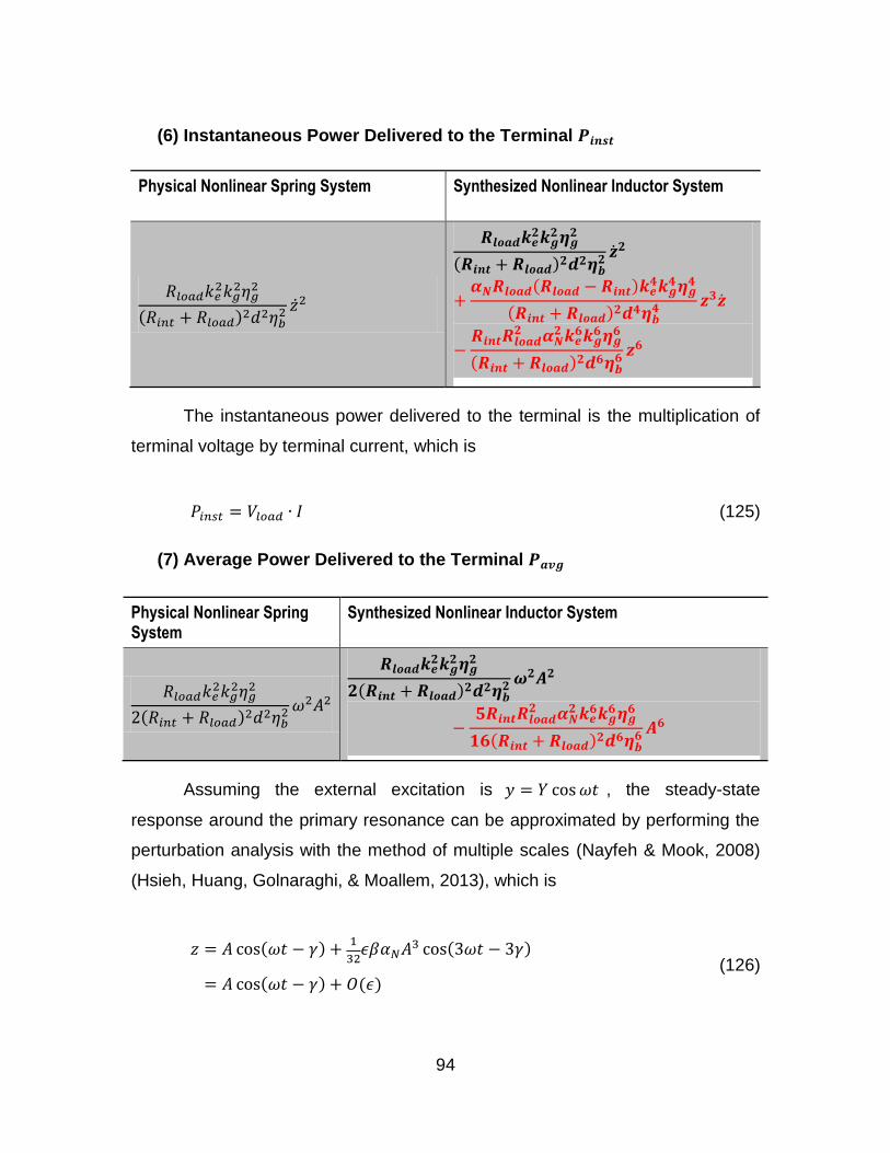
94
(6) Instantaneous Power Delivered to the Terminal
Physical Nonlinear Spring System Synthesized Nonlinear Inductor System
The instantaneous power delivered to the terminal is the multiplication of
terminal voltage by terminal current, which is
(125)
(7) Average Power Delivered to the Terminal
Physical Nonlinear Spring System
Synthesized Nonlinear Inductor System
Assuming the external excitation is , the steady-state
response around the primary resonance can be approximated by performing the
perturbation analysis with the method of multiple scales (Nayfeh & Mook, 2008)
(Hsieh, Huang, Golnaraghi, & Moallem, 2013), which is
(126)

95
where is the amplitude of the dominant approximation term, is a small
parameter and , is the phase shift of the solution, and is a constant.
The average energy harvested per cycle is
∫
(127)
Substituting Eq. (126) into the expression of and calculating based on
Eq. (127), we obtain the expression of , as shown in the above table. Since
the following conditions are always satisfied,
(128)
The average power harvested from the nonlinear synthesized inductor system is
always less than that from the nonlinear physical spring system. The reason is
that part of the power (
in average per cycle) is consumed to
control the circuit for nonlinear inductor realization.
Therefore, it is necessary to utilize the physical spring instead of electrical
elements to provide cubic nonlinearities to the system for the purpose of
maximizing energy harvesting.
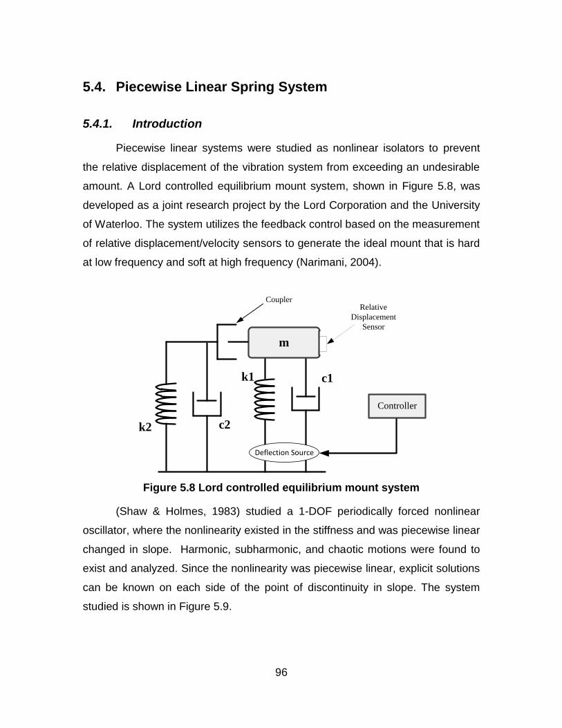
96
5.4. Piecewise Linear Spring System
5.4.1. Introduction
Piecewise linear systems were studied as nonlinear isolators to prevent
the relative displacement of the vibration system from exceeding an undesirable
amount. A Lord controlled equilibrium mount system, shown in Figure 5.8, was
developed as a joint research project by the Lord Corporation and the University
of Waterloo. The system utilizes the feedback control based on the measurement
of relative displacement/velocity sensors to generate the ideal mount that is hard
at low frequency and soft at high frequency (Narimani, 2004).
k1
m
c1
Deflection Source
Controller
Relative
Displacement
Sensor
k2 c2
Coupler
Figure 5.8 Lord controlled equilibrium mount system
(Shaw & Holmes, 1983) studied a 1-DOF periodically forced nonlinear
oscillator, where the nonlinearity existed in the stiffness and was piecewise linear
changed in slope. Harmonic, subharmonic, and chaotic motions were found to
exist and analyzed. Since the nonlinearity was piecewise linear, explicit solutions
can be known on each side of the point of discontinuity in slope. The system
studied is shown in Figure 5.9.

97
x
m
c
y
Displacement
Forc
e
xd
k1
k1+k2
k1
xd
k2
Figure 5.9 1-DOF piecewise linear oscillator and its stiffness property
Inspired by previous investigations on piecewise linear oscillation systems,
the work in this chapter presents a nonlinear energy-regenerative system with
piecewise linear springs to simulate physical nonlinear springs that provide the
cubic nonlinearity, thus improving the bandwidth of power recovery. Figure 5.10
shows the displacement-force curve of the cubic nonlinear spring, with a
piecewise linear fit that can be realized by piecewise linear springs. This means
that the nonlinear relationship between the displacement and the force is
expressed by
(129)
and can be approximated by the piecewise linear function:
(130)
where , , and are the stiffness of the first, second spring, and the
clearance between the second spring and sprung mass. Their values can be
determined by minimizing the mean-square error, MSE( ), between the cubic

98
curve and piecewise linear fitting curve, given , , , and constraint ,
which is the maximum displacement the system can achieve.
Cubic curve
Piecewise linear fitting curve
Displacement
Forc
e
xd
-xd
x
F
k1
k1+k2
k1
k1+k2
Figure 5.10 Cubic curve and piecewise linear fitting curve
5.4.2. System Description and Modeling
Figure 5.11 illustrates the mechanical model of the nonlinear regenerative
suspension system that was considered. Based on the previous proposed model
in Figure 2.1, a second spring set was installed and will interact if the relative
motion of the sprung mass, with respect to the base excitation, exceeds the
clearance Δ. When the amplitude of the relative motion is smaller than the
clearance Δ, the system oscillates at the first stage, where the overall stiffness is
equal to . When the amplitude of the relative motion exceeds the clearance Δ,
the system oscillates at the second stage, where the overall stiffness is equal to
. The stiffness of the system is illustrated in Figure 5.12.

99
y
x
Physical
spring
k1
Variable
electrical resistor
realized by SMR
Base
loadR
Sprung Mass m
DC Motor/
Generator
Ball
screw
d
Shock
absorber
bF
mE
Physical
spring
k2
Coupler
Δ
Δ
Figure 5.11 Mechanical model of the nonlinear regenerative suspension system
Relative displacement
Stiffness
z
k
Δ-Δ
k1
k1+k2
Figure 5.12 Stiffness of the system in terms of the relative displacement
Based on the dynamic modeling in Chapter 2, the governing equation of
the system in Figure 5.11 is expressed as
(131)

100
where
(132)
The other parameters, and , are presented in Table 5.1.
Similar to Section 5.2.2, the dynamic equation of the nonlinear suspension
system, as shown in Eq. (131), can be rewritten as
(133)
where
√
√
√
√
(134)
In order to approximate the system response by using the perturbation
method, we perform the nondimensionalization of the dynamic equation with
respect to the excitation displacement and dimensionless time
.
Assuming the excitation is in the harmonic form , let
(135)

101
Therefore, the dynamic equation (133) is rearranged as
(136)
where
(137)
When the relative displacement stays within the clearance (i.e., | | | |),
the system operates as a linear system based on forced excitation; when the
relative displacement goes beyond the clearance (i.e., | | | |), the system acts
as another linear system with a combined spring constant and an offset on the
excitation by .
5.4.3. Perturbation Analysis
Among the different methods used in perturbation analysis, the method of
averaging is the only one that is applicable when the system contains hard
nonlinearity because it transforms nonlinearities to slow and fast varying
parameters (Nayfeh, 2011).
We are trying to find out the first-order approximation of the solution of Eq.
(136), which is considered to be
(138)
It follows from Eq. (138) that

102
(139)
Using the method of averaging, we assume that parameters and are
slowly varying functions of ; that is, and . In this case, by
differentiating (138), we have
(140)
Comparing Eq. (139) and (140) implies
(141)
By differentiating (139), we have
(142)
Substituting Eq. (142), (139), and (138) into (136) yields
(143)
Eq. (143) can be simplified by substituting
,
[
]
(144)

103
Solving Eq. (141) and (144) leads to
[
]
(145)
[
]
(146)
Since and are assumed to be slowly varying, averages of and
may remain constant over a period [0, 2 ], so that
∫ [
]
(147)
∫ [
]
(148)
where

104
(149)
(
) (150)
since . Performing the integration in Eq. (147) and (148),
we get
(
) (151)
[
]
(152)
Considering that when the steady-state motions of the system occur, the
time derivatives of and are both zero, which means . Thus, Eq.
(151) and (152) lead to
(153)
(154)
Squaring and adding the above two equations, we obtain the solution as

105
[
]
(155)
where
(156)
(157)
(158)
(159)
(160)
Since is a positive real number, it should always satisfy that
(161)
and
[
] (162)
Eq. (155) is an implicit function of frequency response that describes the
relationship between dimensionless amplitude and excitation frequency. We can
also obtain the phase function using Eq. (153) and (154), which is

106
(
) (163)
(1) Stability Analysis
To investigate the stability of the steady-state solution, we derived the
Jacobian matrix of Eq. (151) and (152) at singular points ( )
[
|
|
|
| ]
[
] (164)
where
[ (
)
(
)
] (165)
[
(
)
(
)
(
)
] (166)
By studying the characteristics of eigenvalues of the Jacobian matrix, it
always satisfies that the trace of the Jacobian matrix, . Therefore, the
steady-state motions are unstable when the determinant of the Jacobian matrix,
. That is
(167)

107
Otherwise, the steady-state motions satisfying that are stable.
(2) Frequency Responses
Frequency-response curves of the amplitude and phase of the system’s
relative displacement can be obtained analytically by solving Eq. (155) and (163),
given that , , , ⁄ , and
⁄ . The curves are compared with responses of the linear system and
plotted in Figure 5.13.
0 1 2 3 4 5 6 7 8 9 100
1
2
3
4
5
6
7
8
9
10
Frequency (Hz)
Am
plit
ud
e o
f th
e r
ela
tive
dis
pla
cem
en
t (m
m)
Linear system
Nonlinear system
Nonlinear system(Unstable region)
0 1 2 3 4 5 6 7 8 9 100
0.5
1
1.5
2
2.5
3
3.5
Frequency (Hz)
Ph
ase
of
the
re
lati
ve d
isp
lace
me
nt
Linear system
Nonlinear system
Nonlinear system(Unstable region)
(a) (b)
Figure 5.13 The analytical frequency-response curves of the relative displacement: (a) amplitude and (b) phase
Similar to the frequency-response curves of the system with the nonlinear
variable inductor, the amplitude curve is bent and the phase curve is distorted
due to the effect of the piecewise linear stiffness. The extent of bending is
dependent on the value of and . The portion in green indicates the unstable
states that meet the condition in Eq. (167). Therefore, the steady-state solutions
corresponding to the unstable portion cannot be realized by the system.
In the region where unstable steady-state solutions exist, there are two
stable steady-state solutions: One is nonlinear response, and the other is linear
response. Therefore, two possible stable motions can be observed and the
status is determined by the initial condition. Due to the existence of multiple

108
solutions, a jump phenomenon occurs when the frequency of the excitation is
slowly varied up or down. Figure 5.14 shows the amplitude and phase of the
harmonic response by performing the numerical simulation based on Eq. (151)
and (152). Blue solid curves indicate the trajectories when the frequency sweeps
up and red dot curves indicate the trajectories when the frequency sweeps down.
Arrows in each figure demonstrate the direction of the motion and jump.
0 1 2 3 4 5 6 7 8 9 100
1
2
3
4
5
6
7
8
9
10
Frequency (Hz)
Am
plitu
de
of
the
re
lati
ve
dis
pla
ce
me
nt
(mm
)
Sweep up
Sweep down
0 1 2 3 4 5 6 7 8 9 10
Frequency (Hz)
0
1
2
3
4
5
6
7
8
9
10
Am
plit
ud
e o
f th
e r
ela
tive
dis
pla
cem
en
t (m
m)
0 1 2 3 4 5 6 7 8 9 100
0.5
1
1.5
2
2.5
3
3.5
Frequency (Hz)
Ph
as
e o
f th
e r
ela
tiv
e d
isp
lac
em
en
t
Sweep up
Sweep down
0 1 2 3 4 5 6 7 8 9 10
Frequency (Hz)
0
0.5
1
1.5
2
2.5
3
3.5
Ph
ase
of
the
re
lati
ve d
isp
lace
me
nt
(a) (b)
Figure 5.14 Jump phenomena of relative displacement curves: (a) amplitude and (b) phase
5.4.4. Power Generation and Bandwidth Analysis
Assuming excitation and period of the cycle ⁄ , the
average power flow per cycle is calculated according to Eq. (31)
(
) (168)
Furthermore, the average power can be nondimensionalized as

109
|
|
(
) (169)
By solving Eq. (155) and (169), the frequency-response curves of power
generation can be obtained and plotted in Figure 5.15. Based on this, we can
define the bandwidth of the proposed system and a figure of merit (FoM) for
energy harvesting capability.
0 1 2 3 4 5 6 7 8 9 100
1
2
3
4
5
6
7
8
9x 10
-3
Frequency (Hz)
Ge
ne
rate
d p
ow
er
(no
nd
ime
ns
ion
alize
d)
Linear
Nonlinear (sweep up)
Nonlinear (sweep down)
0 1 2 3 4 5 6 7 8 9 10
Frequency (Hz)
0
20
40
60
80
100
120
140
160
180
Ge
ne
rate
d p
ow
er
(no
nd
ime
nsi
on
aliz
ed
)
(fkD ,PkD)
(fLD ,1/2PkD) (fHD ,1/2PkD)
(fkU ,PkU)
(fLU ,1/2PkU) (fHU ,1/2PkU)
(fkL ,PkL)
(fLL ,1/2PkL) (fHL ,1/2PkL)
Δf of nonlinear system
Δf of linear system
3dB Bandwidth for sweeping down
3dB Bandwidth for sweeping up
Figure 5.15 Frequency-response curve of power generation and bandwidth
The operation bandwidth of a wideband energy harvester was introduced
by (Liu, Badel, Formosa, & Wu, 2015). Due to the characteristics of the
piecewise energy harvester, its bandwidth needs to be analyzed for the
frequency sweep up and sweep down, respectively. As shown in Figure 5.15, the
3 dB bandwidth for sweeping up can be found from the peak-power point
( ) and two half peak-power points ( ) and ( ).
Similarly, the bandwidth for sweeping down can be obtained from three
corresponding parameters ( ), ( ), and ( ). Therefore,

110
the total operation bandwidth is defined to cover the favorable range for both
sweeping up and sweeping down responses, which is
(170)
The bandwidth of the linear system is also depicted based on three points
( ), ( ), and ( ) and is expressed as .
To examine the energy harvesting capability of the proposed system, a
new FoM is introduced based on two critical factors: operation bandwidth, , as
described in Eq. (170); and expectation of power generation across the whole
excited frequency range, , which can be expressed as
∫
(171)
where and are upper and lower bounds of the excitation frequency.
and are the average power generation at a certain frequency
for sweeping up and down situations, respectively. and denote the
probability to obtain a response in frequency sweeping up and down, which
satisfy that
(172)
Therefore, the energy harvesting FoM can be defined as
(173)

111
provides a systematic methodology to evaluate the system’s
energy harvesting performance. It also implies that the sum of the average power
generation and the ratio of the operation bandwidth to the whole frequency range
make a coupling contribution to the evaluation.
5.4.5. Experimental Setup and Test Results
To validate the analytical results from the previous theoretical analysis by
the perturbation method, a prototype was fabricated and an experimental test-
bed was developed to test its nonlinearity and performance.
(1) Prototype Design and Test-Bed
Based on the prototype, as shown in Figure 2.2, a second pair of die
springs with higher stiffness (i.e., 116109 N/m) was installed on top of the first
pair of springs and a pair of couplers was set up around the sprung mass, as
depicted in Figure 5.16. Figure 5.17 indicates the test-bed setup based on the
designed prototype. All the other hardware descriptions are mentioned in
Chapter 2.4, and the values of corresponding parameters are listed in Table 2.1.

112
Base excitation
DC motor/generator
Coupler
Sprung mass
Ball screw mechanism
Piecewise springs
Figure 5.16 CAD prototype of the regenerative suspension system with piecewise springs
Sprung mass
Piecewise SpringsBall screw
Coupler
Planetary gearhead
String potentiometer
DC motor/generator
Accelerometer
Hydraulic shaker
Figure 5.17 Experimental test setup for the regenerative suspension system with piecewise springs
(2) Frequency Responses
This experiment was performed to study frequency responses of the
system based on harmonic excitations and compare its energy harvesting

113
performance with that of the linear system. After applying a sweeping sinusoidal
excitation slowly increased from 2 Hz to 10 Hz and also decreased from 10 Hz to
2 Hz, the responses of the system were measured and analyzed. During the test,
the amplitude of the excitation was held constant at 7 mm, and the clearance
between the coupler and sprung mass was 4 mm. The value of the load resistor
was chosen as 490 Ω. At each frequency step, the amplitude of the relative
displacement was captured by the string potentiometer, the absolute acceleration
of the sprung mass was measured by the accelerometer, and the terminal
voltage of the load resistant was read and recorded by the dSPACE DS1103
system. The generated power was calculated by the load resistance and its
terminal voltage at different frequencies. Figure 5.18 shows the frequency
responses of the system, where experimental results are indicated by dotted
lines compared to the numerical simulation results depicted by solid lines.
2 3 4 5 6 7 8 9 100
5
10
15
Frequency (Hz)
Am
plitu
de
of
rela
tiv
e d
isp
lac
em
en
t (m
m)
Experimental (Linear)
Experimental (Nonlinear-sweep up)
Experimental (Nonlinear-sweep down)
Numerical (Linear)
Numerical (Nonlinear-sweep up)
Numerical (Nonlinear-sweep down)
2 3 4 5 6 7 8 9 10
Frequency (Hz)
Am
plit
ud
e o
f th
e r
ela
tive
dis
pla
cem
en
t (m
m)
5
10
15
0
1
2
3
4
5
(a)

114
2 3 4 5 6 7 8 9 100
5
10
15
20
25
30
Frequency (Hz)
Av
era
ge
of
ge
ne
rate
d p
ow
er
(W)
Experimental (Linear)
Experimental (Nonlinear-sweep up)
Experimental (Nonlinear-sweep down)
Numerical (Linear)
Numerical (Nonlinear-sweep up)
Numerical (Nonlinear-sweep down)
2 3 4 5 6 7 8 9 10
Frequency (Hz)
5
10
15
0
20
25
30
Ave
rage
of
the
Ge
ne
rate
d p
ow
er
(W)
(b)
Figure 5.18 Experimental frequency responses of the regenerative suspension system with piecewise springs: (a) relative displacement and
(b) generated power
Referring to Figure 5.18 (a), when the excitation frequency increases, the
relative displacement increases the same as the linear system until the moving
mass hits the couplers at point 1. From this moment, the increasing rate changes,
and the amplitude keeps increasing until it reaches point 2, where the amplitude
suddenly and dramatically decreases to point 3. Then the system becomes linear,
and no more rattling occurs.
As the excitation frequency decreases, the system acts as linear from
point 3 to point 4, where the moving mass hits the couplers again and the rattling
begins. The amplitude of the relative displacement rapidly increases to point 5
and begins to decrease to point 1, where the mass stops hitting the couplers and
the system resumes as linear.
From the results, it can be seen that the regenerative suspension system
with piecewise springs provides a jump phenomenon, which is a typical feature of
the cubic nonlinearity, as shown in Figure 5.6. Therefore, the bandwidth of the

115
regenerative suspension system is extended by utilizing the piecewise linear
springs.
The comparison between the linear and nonlinear systems is indicated in
Figure 5.19. The results reveal the advantages and disadvantages of the
nonlinear suspension system. By using piecewise springs, the system’s response
bandwidth is widened, thus improving its power generation capability. But the
relative displacement and absolute acceleration are both increased, which
means the control performance of the system is sacrificed as a result. The trade-
off between dynamic control and power generation should be considered when
applying the nonlinear technique.
Figure 5.19 Comparison between linear and nonlinear systems
(3) Power Generation Efficiency
According to Section 2.3.4, mechanical efficiency, electrical efficiency, and
overall efficiency of power generation are defined. The experimental results from
4 Hz to 8 Hz where nonlinearities exist were obtained, as displayed in Figure
5.20.
0
2
4
6
8
10
12
14
16
18
20
RMS of relativedisplacement
(mm)
RMS of absoluteacceleration
(m^2/s)
Average ofgenerated power
(w)
Linear
Nonlinear (Frequencyincreased)
Nonlinear (Frequencydecreased)

116
4 5 6 7 80.498
0.499
0.5
0.501
0.502
0.503
4 5 6 7 80.6
0.7
0.8
0.9
1
4 5 6 7 80.32
0.35
0.38
0.41
0.44
0.47
4 5 6 7 8Frequency (Hz)
0.498
0.499
0.5
0.501
0.502
0.503
Me
chan
ical
Eff
icie
ncy
0.32
0.35
0.38
0.41
0.44
0.47
Ove
rall
Effi
cie
ncy
Electrical Efficie
ncy
0.6
0.7
0.8
0.9
1
Overall Efficiency
Electrical EfficiencyMechanical Efficiency
Figure 5.20 Mechanical, electrical, and overall efficiency of power generation
Results show that the mechanical efficiency maintains at around 50% and
the electrical efficiency ranges from 66% to 93%. The overall efficiency of power
generation was obtained within the range of 33% to 46%, and the highest
efficiency was obtained around 6 Hz.
(4) Comparison of FoM for energy harvesting performance
FoMs of the proposed energy harvesting system and linear system were
calculated, and corresponding values are listed in Table 5.2, along with
parameters and . It is assumed that the probability of frequency increase
and frequency decrease is equal, which means .
Table 5.2 Comparison of FoMs for linear and nonlinear energy harvesters
(Hz) (W) (W Hz)
Linear system 1.39 1.03 1.432
Nonlinear system 4.40 5.91 26.004
Figure 5.18 and Table 5.2 confirm that both the amplitude of power
generation across the excitation frequency range and operation bandwidth are

117
increased due to the piecewise linear stiffness. Thus, the FoM of the system’s
energy harvesting performance is improved significantly.
To analyze system parameters’ effect on FoM for energy harvesting, we
obtained frequency responses of the energy harvester based on different values
of the electrical load resistor (i.e., ) and coupler clearance (i.e., ). The
corresponding FoMs were calculated and compared, as shown in Figure 5.21
and Figure 5.22.
1 2 3 4 52
3
4
5
6
1 2 3 4 52
3
4
5
6
1 2 3 4 55
10
15
20
25
30
150 200 300 400 490
Load resistor (Ohm)
5
10
15
20
25
30
FoM
(W·H
z)
2
3
4
5
6
Δ f
(H
z)E p
(W
)
Δ f
Ep
FoM
Figure 5.21 FoM for different values of load resistor
1 2 3 41
2
3
4
5
1 2 3 42
4
6
8
10
1 2 3 48
13
18
23
28
3 4 5 6
Coupler clearance (mm)
8
13
18
23
28
FoM
(W·H
z)
1
2
3
4
5
Δ f
(H
z)
E p (
W)
2
4
6
8
10
FoM
Ep
Δ f
Figure 5.22 FoM for different values of coupler clearance

118
By varying and , we find some characteristics of the proposed
energy harvester as follows:
Higher load resistor provides larger bandwidth and higher average of power generation, thus increasing the FoM for energy harvesting;
Increasing coupler clearance improves bandwidth but decreases average of power generation. There is an optimum value of clearance setup to obtain the best FoM for energy harvesting.
(5) Experimental Results of Stochastic Excitation
The system was also examined by applying a stochastic excitation which
was generated as a standard road roughness in the time domain to simulate a
City situation (See Table 4.1). The excitation profile is shown in Figure 5.23.
0 2 4 6 8 10 12 14 16 18 20-100
-80
-60
-40
-20
0
20
40
60
80
100
Time (sec)
Bas
e e
xcit
atio
n a
nd
ab
solu
te
dis
pla
cem
en
t (m
m)
Figure 5.23 Stochastic road profile to simulate a City situation
Figure 5.24 through Figure 5.26 show the system responses, including
relative displacement, absolute acceleration, and generated power in the time
domain, compared with the linear system responses. The results show that the
control of relative displacement and the power generation capability both
improved, while the control of absolute acceleration declined. Therefore, from the
energy harvesting point of view, piecewise linear springs improve the system’s

119
performance and can be a physical alternative to the nonlinear variable inductor.
On the other hand, it should be noted that the system’s control performance is
sacrificed by utilizing piecewise linear springs so it must be maintained at an
acceptable level. The balance between dynamic control and power generation
may vary in different driving situations and depending on the user’s demand.
0 2 4 6 8 10 12 14 16 18 20-8
-6
-4
-2
0
2
4
6
8
Time (sec)
Am
plit
ud
e o
f re
lati
ve d
isp
lace
me
nt
(mm
)
Linear systemNonlinear system
(a) (b)
Figure 5.24 Relative displacement of linear and nonlinear systems
-50
-40
-30
-20
-10
0
10
20
30
40
50
Am
plit
ud
e o
f ab
solu
te a
cce
lera
tio
n
(m/s
2)
0 2 4 6 8 10 12 14 16 18 20Time (sec)
Linear systemNonlinear system
(a) (b)
Figure 5.25 Absolute acceleration of linear and nonlinear systems
0
0.5
1
1.5
2
2.5
3
RMS of relativedisplacement (mm)
Linearsystem
Nonlinearsystem
6.5
7
7.5
8
8.5
9
9.5
RMS of absoluteacceleration (m/s^2)
Linearsystem
Nonlinearsystem
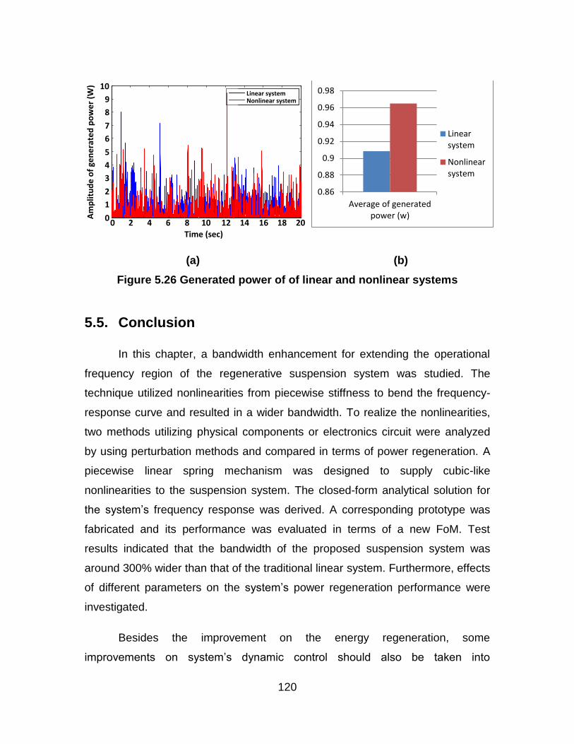
120
0
1
2
3
4
5
6
7
8
9
10A
mp
litu
de
of
gen
era
ted
po
we
r (W
)
0 2 4 6 8 10 12 14 16 18 20Time (sec)
Linear systemNonlinear system
(a) (b)
Figure 5.26 Generated power of of linear and nonlinear systems
5.5. Conclusion
In this chapter, a bandwidth enhancement for extending the operational
frequency region of the regenerative suspension system was studied. The
technique utilized nonlinearities from piecewise stiffness to bend the frequency-
response curve and resulted in a wider bandwidth. To realize the nonlinearities,
two methods utilizing physical components or electronics circuit were analyzed
by using perturbation methods and compared in terms of power regeneration. A
piecewise linear spring mechanism was designed to supply cubic-like
nonlinearities to the suspension system. The closed-form analytical solution for
the system’s frequency response was derived. A corresponding prototype was
fabricated and its performance was evaluated in terms of a new FoM. Test
results indicated that the bandwidth of the proposed suspension system was
around 300% wider than that of the traditional linear system. Furthermore, effects
of different parameters on the system’s power regeneration performance were
investigated.
Besides the improvement on the energy regeneration, some
improvements on system’s dynamic control should also be taken into
0.86
0.88
0.9
0.92
0.94
0.96
0.98
Average of generatedpower (w)
Linearsystem
Nonlinearsystem

121
consideration. Compared to the passive suspension system, the semi-active
suspension system can provide a better control performance, so a study on a
self-powered regenerative Skyhook control is demonstrated in the next chapter.

122
Chapter 6. Regenerative Skyhook Control for the Hybrid Vehicle Suspension System
In this chapter, the hybrid suspension system, a self-powered suspension
system with capabilities of energy harvesting and active/semi-active control, is
presented. A modified Skyhook control strategy is designed to offer better control
performance while recapturing energy from the excitation input. Two operational
modes, including regeneration mode and control mode, are studied. An intelligent
strategy to manage the switching between two modes is also proposed. Based
on the rule, the system can be prevented from running out of energy. Therefore,
unlike the traditional active and semi-active suspension systems, the control of
the hybrid suspension system is independent of external energy. The numerical
simulation is conducted, and the results reveal that the system performs not only
as well as the active suspension system but saves energy at the same time.
6.1. Control Methods for Vehicle Suspension Systems
In this section, passive damping control and several active/semi-active
control methods are examined (Shen, Golnaraghi, & Heppler, 2006). The control
performances of different methods are compared through the numerical
simulation. To fully understand the effects of the examined control strategies, the
transient response and steady-state response are evaluated based on bump
excitation and harmonic excitation, respectively.

123
6.1.1. Active Skyhook Control
Because one of the major performance metrics of a vehicle suspension
system is the minimization of acceleration of the sprung mass, (Karnopp, Crosby,
& Harwood, 1974) proposed the Skyhook method, which attempts to limit the
movement of the sprung mass through the introduction of a fictitious damper
between the mass and a fixed inertial reference. The schematic structure of a
typical Skyhook control system model is shown in Figure 6.1.
ms
x
yk c1
c2
Figure 6.1 Schematic structure of a typical Skyhook control system model
This control method is achieved in practice through use of an actuator in a
fully-active system. Considering a 1-DOF suspension system equipped with a
Skyhook damper, the damping force can be found as follows:
(174)
where is the damping coefficient of the Skyhook damper and is the velocity
of the sprung mass. However, conventional dampers and the electrical damper
proposed in this thesis can only generate the damping force proportional to the
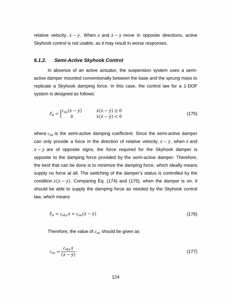
124
relative velocity, . When and move in opposite directions, active
Skyhook control is not usable, as it may result in worse responses.
6.1.2. Semi-Active Skyhook Control
In absence of an active actuator, the suspension system uses a semi-
active damper mounted conventionally between the base and the sprung mass to
replicate a Skyhook damping force. In this case, the control law for a 1-DOF
system is designed as follows:
(175)
where is the semi-active damping coefficient. Since the semi-active damper
can only provide a force in the direction of relative velocity, , when and
are of opposite signs, the force required for the Skyhook damper is
opposite to the damping force provided by the semi-active damper. Therefore,
the best that can be done is to minimize the damping force, which ideally means
supply no force at all. The switching of the damper’s status is controlled by the
condition . Comparing Eq. (174) and (175), when the damper is on, it
should be able to supply the damping force as needed by the Skyhook control
law, which means
(176)
Therefore, the value of should be given as
(177)

125
It can be seen from Eq. (177) that when the relative velocity is very small,
the required damping coefficient can be extremely large. However, in reality, the
damping coefficient is limited by the physical constraints of the semi-active
damper, which are upper and lower bounds, and . Thus, according to
(Liu, Waters, & Brennan, 2005), the feasible damping coefficient can be rewritten
as
( (
))
(178)
The control law described in Eq. (178) is continuously variable. To simplify
the operation, an on-off control scheme has been proposed which acts as a
conventional passive damper, and the damping coefficient is switched between
the maximum and minimum values of the damper (Karnopp, Crosby, & Harwood,
1974). The control law can be written as
(179)
The difference between continuous Skyhook control and on-off Skyhook
control is that the former method attempts to provide the same amplitude and
phase as those of the active Skyhook control when the damper is enabled.
However, its performance is constrained by the limitations of the physical device.
The latter method can only guarantee that the damping force remains the same
sign as the active Skyhook damper. Experiments show that both semi-active
Skyhook control methods provide comparable performance and gain big
improvements over the passive suspension system (Ivers & Miller, 1989).

126
6.1.3. Semi-Active Rakheja-Sankar Control
Research by (Rakheja & Sankar, 1985) found that the damping force
provided by a passive damper tends to increase the acceleration of the
suspended mass when it is in the same direction as the spring force. Ideally, a
semi-active damper should provide no damping force or minimized damping in
this situation. To overcome this effect, (Alanoly & Sankar, 1987) suggested that
the damping force should be set off when in the same direction as the spring
force, and should cancel out the spring force when in the opposite direction. An
on-off control strategy was designed accordingly and mathematically expressed
as follows:
(180)
Much as the Skyhook method was simplified to provide an on-off control
since it is difficult to make the damping force fully follow the spring force due to
the limitation of the physical damper in practice, a new form of the Rakheja-
Sankar control strategy that does not require following the spring force was
created as
(181)
6.1.4. Modified Skyhook Control
By utilizing a control method called double-band hysteresis current control
(DB-HCC), a SMR power electronic circuit was developed that is capable of
providing either positive or negative damping by controlling the electric current to
alternate between regenerative and motoring modes (Hsieh, Huang, Golnaraghi,
& Moallem, 2016). Therefore, the damper can supply a negative force from a

127
negative damping coefficient, . In this case, a modified Skyhook control
algorithm was proposed and can be written as
(182)
when , is determined for either better vehicle control (i.e.,
negative force) or energy harvesting (i.e., zero force), respectively. This is due to
the negative direction of current results in power consumption of the electrical
load. The Skyhook damping coefficient can be realized by synthesizing a
tunable load resistance, , by the proposed SMR power electronics.
Specifically, it can be calculated referring to Eq. (29)
(183)
The desired positive or negative damping force can be provided by tuning
the circuit current , in terms of the reference current . By recalling Eq. (27), in
order to implement the control algorithm in the electrical domain by the SMR, the
current should be controlled to the following reference current:
(184)
When the stored energy is enough to supply a negative current, the
damper provides active Skyhook control to maintain the best dynamic control.
Otherwise, it acts as a semi-active Skyhook damper.

128
6.1.5. Comparison of Different Control Methods
Numerical simulations are conducted in this section to compare the control
performance of different control methods, including passive control, semi-active
Skyhook control, semi-active Rakheja-Sankar control, and modified Skyhook
control. The evaluated system is the proposed 1-DOF regenerative suspension
system whose dynamic equation follows Eq. (42) and (43).
During the simulation spring constant does not vary, while the damping
coefficient is adjusted by the control strategy and can have a value of either
or . In the following simulation, the value of the load
resistance is selected as 40 to achieve the optimal damping for energy
harvesting, as introduced in Chapter 3. The testing is conducted under the
following assumptions:
- The damper is capable of a value of zero and is able to instantly change values;
- The spring and damper are operating linearly;
- The modified Skyhook control is able to provide negative damping force as needed;
- The relative displacement sensor and the absolute acceleration sensor are operating with perfect accuracy, linearly and instantaneously;
- Ride comfort is used as the criterion of control performance so the absolute acceleration of the sprung mass is compared based on different control methods.
(1) Transient Response
The test of the system’s transient response utilizing different control
methods is based on bump excitation. Assuming a vehicle is running through a
speed hump that is 350 mm wide and 50 mm high and the vehicle speed is kept
at 12.6 km/h, the situation is indicated in Figure 6.2.

129
Figure 6.2 Situation of a vehicle running through a speed hump2
The bump excitation can be expressed mathematically as
(185)
and the profile of the excitation is shown in Figure 6.3.
Time (sec)Am
plit
ud
e o
f b
um
p e
xcit
atio
n (
m)
0 0.01 0.02 0.03 0.04 0.05 0.06 0.07 0.08 0.09 0.10
0.01
0.02
0.03
0.04
0.05
Figure 6.3 Profile of the bump excitation
The simulation results are shown in Figure 6.4. All the semi-active and
active control methods can provide better control of the bump excitation.
Specifically, both semi-active control methods made 10.3% and 11.2%
decreases in the first and second peak acceleration (Point 1 and Point 2)
compared with the passive system. Furthermore, Skyhook control decreased
2 According to product specifications from JMP Holdings Pty Ltd.

130
28.4%, and Rakheja-Sankar control decreased 16.2% in the third peak
acceleration (Point 3). The modified Skyhook control method contributed to
11.3%, 56.8%, and 43% decreases, respectively. Due to the discontinuity of the
excitation acceleration at Point 3, a sudden drop happened from Point 3 to Point
4, where all the control methods performed worse than the passive system.
Overall, the modified Skyhook strategy offers the best control performance in
dealing with the bump excitation.
0 0.05 0.1 0.15 0.2 0.25 0.3 0.35 0.4 0.45 0.5-60
-40
-20
0
20
40
60
Time [sec]
Ab
solu
te A
cce
lera
tio
n [
m/s
2]
4
3
2
1
Passive system
Skyhook control
Rakheja-Sankar control
Modified Skyhook control
Figure 6.4 Absolute acceleration responses of the system with different control methods based on bump excitation
(2) Steady-State Response (Frequency Response)
The test of the system’s steady-state response based on different control
methods is examined in terms of the system’s frequency response over 2 Hz to 9
Hz with base excitation amplitude of 20mm. The curves of the system’s absolute
acceleration transmissibility are plotted in Figure 6.5. Results show that both
semi-active control methods did not improve performance in the low frequency
region (i.e., excitation frequency lower than natural frequency) and the Rakheja-
Sankar method even performed worse than the passive system. However, in the
high-frequency region where excitation frequency is higher than natural

131
frequency, both semi-active controls obtained lower absolute acceleration than
the passive system. Apparently, the modified Skyhook control strategy
contributed to a significant reduction of absolute acceleration over the whole
frequency range, thus achieving the best control performance. The RMS values
of the absolute acceleration transmissibility are calculated and plotted in Figure
6.6, which quantifies the control performance by using different control methods
(lower is better).
2 3 4 5 6 7 8 90
200
400
600
800
1000
1200
1400
1600
1800
2000
Frequency [Hz]
Ab
solu
te A
cce
lera
tio
n T
ran
smis
sib
ility
[1
/s2]
Passive system
Skyhook control
Rakheja-Sankar control
Modified Skyhook control
Figure 6.5 Absolute acceleration responses of the system with different control methods based on harmonic excitation

132
Figure 6.6 RMS of absolute acceleration transmissibility for different control methods
6.2. Operation Modes for the Hybrid Suspension System
In this section, a decision strategy for mode switch between energy
harvesting and dynamic control is proposed. The amount of the energy required
for the active control is calculated, and the conditions under which the self-
powered system would be feasible are studied.
6.2.1. Schematic of the Hybrid Suspension System
The schematic of the proposed hybrid suspension system is shown in Figure
6.7. The system consists of two operating modes: regeneration mode and control
mode.
In regeneration mode ( ), the system supplies the positive
damping force while harvesting real power from the regenerative vehicle
suspension. In control mode ( ), the system provides either negative
(i.e. consuming energy) or zero (i.e. no energy flow) damping force that depends
0
200
400
600
800
1000
1200
RMS of absolute accelerationtransmissibility
Passive
Semi-active Skyhook
Semi-active R-S
Modified Skyhook

133
on the relationship between desired energy and stored energy, and the damper
alternates between active and semi-active while the suspension is under control.
DC Motor/Generator
Power Source
When induced energy larger than battery energy (Em>Eb)
When battery energy larger than induced energy (Em<Eb)
Hybrid suspension system
Regeneration mode
Control mode
Battery
Harvesting energy Draining energy
Em
Eb
Figure 6.7 Schematic of the hybrid suspension system
6.2.2. Conditions of Self-Powered Control
Assuming the induced back-EMF voltage by the electrical motor/generator
is , the instantaneous electrical power generated by the damper is
(
)
(186)
Thus, the cumulative generated energy is calculated as
∫
(187)
When the active Skyhook control is set on, the desired negative damping
force is given by
(188)

134
Since is to be provided by the DC motor, the desired power to supply
the damping force can be calculated by
(189)
Eq. (189) shows that the power is always negative to provide a negative
damping force, which means the damper is draining power in this case.
Therefore, the required energy during the time will be
(190)
When the stored energy in the battery, , is higher than the desired
energy for the active control, , the system is able to provide enough power for
the damping force without external energy.
The algorithm to determine the suspension system operating with the self-
powered regenerative Skyhook control strategy is described in Figure 6.8.

135
Yes
No
Check battery energyEgen
Calculate desired damping force
Fd
Is desired dampingforce positive?
Fd > 0 ?
Regeneration mode
Control mode
Calculate desired powerPd
Calculate desired energyEd
Is battery energyavailable?Eeng > Ed ?
Yes
No
Apply positive damping force Fd to the suspension
Cut off circuit Fd = 0
Apply negative damping force Fd to the suspension
Calculate instantaneous power generated Pgen
Calculate instantaneous power consumed Pd
Calculate energy generated during time dt
dE = Pgen x dt
Calculate energy consumed during time dt
dE = Pd x dt
No energy flow during time dtdE = 0
Update energy in the batteryE = E + dE
Figure 6.8 Algorithm for determining the suspension system operating with the self-powered regenerative Skyhook control strategy

136
6.3. Numerical Simulation Results
To verify the feasibility and effectiveness of the suspension system
utilizing the proposed self-powered regenerative Skyhook control strategy, the
numerical simulation was implemented in Matlab environment to evaluate the
performance of the controlled system. The values of the main parameters for the
quarter-car suspension system were selected as in Table 2.1. The capacity of the
battery was 24 kWh, and initially it was assumed that the battery was fully
discharged. The excitation profile is a harmonic waveform whose amplitude is 20
mm, and frequency is sweeping from 2 Hz to 9 Hz with increments at 0.1 Hz/s for
70 s. The profile of the excitation is shown in Figure 6.9.
0 1 2 3 4 5 6 7-0.025
-0.02
-0.015
-0.01
-0.005
0
0.005
0.01
0.015
0.02
0.025
Time [sec]
Exci
tati
on
pro
file
[m
]
Figure 6.9 Excitation profile with frequency sweeping from 2 Hz to 9 Hz
Figure 6.10 (a) indicates the absolute acceleration of the sprung mass for
passive control, semi-active Skyhook control, externally-powered modified
Skyhook control, and self-powered modified Skyhook control. The zoomed-in
waveform between 1 s to 3 s is shown in Figure 6.10 (b). The instantaneous
power of the battery and its cumulative energy the whole time are depicted in
Figure 6.11.

137
0 1 2 3 4 5 6 7-100
-80
-60
-40
-20
0
20
40
60
80
100
Time [sec]
Ab
solu
te A
cce
lera
tio
n [
m/s
2]
Passive
Semi-active Skyhook
Modified Skyhook
Modified Skyhook (self-powered)
(a)
1 1.2 1.4 1.6 1.8 2 2.2 2.4 2.6 2.8 3-40
-30
-20
-10
0
10
20
30
40
Time [sec]
Abs
olut
e A
ccel
erat
ion
[m/s
2 ]
Passive
Semi-active Skyhook
Modified Skyhook
Modified Skyhook (self-powered)
(b)
Figure 6.10 Absolute acceleration of the sprung mass for passive and controlled systems: (a) 0 - 7 s and (b) zoomed-in at 1 s - 3 s

138
0 1 2 3 4 5 6 7-60
-40
-20
0
20
40
60
Time [sec]
Inst
anta
ne
ou
s p
ow
er
[W]
0 1 2 3 4 5 6 70
1
2
3
4
5
6
7
8
Time [sec]
Cu
mu
lati
ve e
ne
rgy
[J]
(a) (b)
Regeneration mode
Control mode
Figure 6.11 Instantaneous power and cumulative energy of the battery
Referring to Figure 6.10, the self-powered modified Skyhook control
method performed as well as the externally-powered modified Skyhook control
method before 2 Hz. After 2 Hz, the performance of the self-powered modified
Skyhook control appears moderate, between the externally-powered modified
Skyhook control and semi-active Skyhook control. Figure 6.11 (a) shows how the
controller switched between regeneration mode and control mode. Figure 6.11 (b)
indicates that the energy reached maximum before 2 Hz and reduced gradually
afterwards, which explains why the control performance declined after 2 Hz.
Apparently, the self-powered modified Skyhook control strategy proposed in this
work outperformed semi-active control methods, and its property of external
power independence is a big advantage over active control methods.
6.4. Conclusion
In this chapter, a regenerative Skyhook control strategy was demonstrated
and compared with other damping control methods based on bump and
harmonic excitations. The strategy was able to provide energy harvesting and
dynamic control simultaneously. An algorithm was described in determining two
operating modes for the suspension system. It was demonstrated, through the

139
numerical simulation, that the proposed control strategy was able to operate
using self-generated power and outperformed the conventional semi-active
control methods. The next chapter concludes the overall work proposed in this
thesis, and outlines potential future works.

140
Chapter 7. Conclusion and Future Work
7.1. Conclusion
At present, a series of energy and environmental issues caused by
excessive vehicles have been a serious concern. Large amounts of energy are
consumed, but only a small ratio of that is utilized to drive a car. One important
reason is that much energy has been wasted by the shock absorber in the
suspension system. The traditional suspension system contains a viscous shock
absorber that dissipates road energy into waste heat. On the other hand, to
maintain better ride comfort for passengers, conventional passive suspension is
not suitable because it cannot accomplish variable control objectives. Various
sophisticated suspension control strategies, including active and semi-active
control methods, have been proposed to improve the control performance;
however, they consume a certain level of electrical power.
The main objective of the research in this thesis is to regenerate the waste
energy from the vehicle suspension and enable the dynamic control of the
vehicle sprung mass simultaneously. Motivated by the demand of both energy
saving and dynamic control, an energy-regenerative vehicle suspension system
is developed to meet the purpose. The proposed system not only harvests
vibrational energy induced by road irregularities, but also provides adjustable
levels of damping in the electrical domain to achieve a suitable ride comfort. The
contributions of this thesis are summarized as follows:

141
1. A 1-DOF energy-regenerative suspension system was designed, and
its mathematical modeling was derived. A small-scale proof-of-concept
prototype was manufactured, and a test-bed was established to verify
its effectiveness. Experimental results were obtained and compared
with numerical simulation results. The results showed that the
proposed system is capable of providing appropriate damping control
and regenerating energy from external excitation.
2. Two systematic optimization methodologies for parameters design of
the suspension system were proposed, with respect to harmonic
excitation and ISO standard road profile. Both methods presented
graphical optimization rules in terms of RMS of the absolute
acceleration transmissibility and average of the power generation
transmissibility. The experimental results demonstrated that the
optimization strategies well predicted the system performance under
different conditions and were effective when used as the guideline for
optimal design of the regenerative suspension system.
3. A nonlinear strategy for the purpose of extending the suspension
system’s operational frequency region was implemented. The
technique utilized cubic nonlinearity to introduce a Duffing equation to
the system’s dynamic modeling. Thus, it overcomes the limited
bandwidth of the linear resonant generator. A piecewise linear spring
system was used to physically realize nonlinear phenomena, and it
significantly improved the energy harvesting capability of the
suspension system according to the experiment results.
4. A regenerative Skyhook control strategy was proposed for the
combination of power regeneration and active Skyhook control. The
possibility of the strategy’s external power independence was
examined, and a mode switch algorithm was designed to guarantee

142
that the Skyhook control operates using the self-generated energy.
Numerical simulations were conducted to verify the effectiveness of the
proposed strategy, which therefore mitigates the contradiction between
control deficiency of passive suspension control and power
consumption of active suspension control.
7.2. Future Work
Based on the completed work and results obtained from this research,
additional works are taken into consideration and expected to be accomplished in
the future, as follows:
1. This work has shown a strong relationship between RMS analysis and
stochastic-based analysis. The expectation of the stochastic response
has been derived from the RMS information. In future work, the explicit
relationship between RMS results for the harmonic excitation and
results for the stochastic excitation should be investigated. Similar
method can be utilized to analyze the system response based on
bump excitation, by transforming the response in time-domain to the
sequence in frequency-domain.
2. The cubic nonlinearity introduced in this thesis is able to extend the
system’s bandwidth; however, it also sacrifices the control
performance, especially at high frequency. To maintain ride comfort
and road handling at an acceptable level, some advanced optimization
strategies should be investigated to deal with the trade-off between
power regeneration and ride comfort/road handling of the nonlinear
suspension system using perturbation methods.
3. Currently the nonlinearities are added physically to the system by
using piecewise linear spring. However, considering the size and

143
weight would be increased due to additional components, future work
should investigate on introducing nonlinearities electronically.
4. In this work, feasibility of the regenerative Skyhook control strategy
using self-power is examined by numerical simulations but lacks
experimental verification. The experimental test on the regenerative
Skyhook control strategy should be implemented for future work.

144
References
Adcock, I. (2012). Michelin's innovative active wheel. Retrieved from http://www.roadandtrack.com/car-shows/news/a21961/michelins-innovative-active-wheel-2012-goodwood-festival-of-speed-36312/.
Adhikari, S., Friswell, M. I., & Inman, D. J. (2009). Piezoelectric energy harvesting from broadband random vibrations. Smart Materials and Structures, 18(11), 115005.
Alanoly, J., & Sankar, S. (1987). A new concept in semi-active vibration isolation. Journal of Mechanical Design, 109(2), 242-247.
Anderson, T. J., Nayfeh, A. H., & Balachandran, B. (1996). Coupling between high-frequency modes and a low-frequency mode: Theory and experiment. Nonlinear Dynamics, 11(1), 17-36.
Appleyard, M., & Wellstead, P. E. (1995). Active suspensions: Some background. In Control Theory and Applications, IEE Proceedings, IET, 142(2), 123-128.
Arzanpour, S., Eslaminasab, N., Shubert, B., Narimani, A., & Golnaraghi, M. F. (2006). A novel technique for frequency and time optimization of automotive engine mount parameters. ASME International Mechanical Engineering Congress and Exposition, (pp. 1613-1620).
Ashmore, S. C., & Hodges, H. C. (1992). Dynamic force measurement vehicle (DFMV) and its application to measuring and monitoring road roughness. In J. J. Henry, & J. C. Wambold, Vehicle, Tire, Pavement Interface (pp. 69-69). ASTM Special Technical Publication 1164.
Barton, D. A., Burrow, S. G., & Clare, L. R. (2010). Energy harvesting from vibrations with a nonlinear oscillator. Journal of Vibration and Acoustics, 132(2), 021009.
Bastow, D., Howard, G., & Whitehead, J. P. (2004). Car suspension and handling (4th ed.). Warrendale, PA: SAE international.

145
Beeby, S. P., Torah, R. N., Tudor, M. J., Glynne-Jones, P., O'Donnell, T., Saha, C. R., et al. (2007). A micro electromagnetic generator for vibration energy harvesting. Journal of Micromechanics and Microengineering, 17(7), 1257.
Biglarbegian, M. M., & Golnaraghi, F. (2006). Intelligent control of vehicle semi-active suspension systems for improved ride comfort and road handling. In Fuzzy Information Processing Society. NAFIPS 2006. Annual meeting of the North American (pp. 19-24). IEEE.
Biglarbegian, M. M., & Golnaraghi, F. (2008). A novel neuro-fuzzy controller to enhance the performance of vehicle semi-active suspension systems. Vehicle System Dynamics, 46(8), 691-711.
Bogsjö, K., Podgórski, K., & Rychlik, I. (2012). Models for road surface roughness. Vehicle System Dynamics, 50(5), 725-747.
Bolandhemmat, H. C., & Golnaraghi, F. (2010). Development of a systematic and practical methodology for the design of vehicles semi-active suspension control system. Vehicle System Dynamics, 48(5), 567-585.
Bose Suspension System. (n.d.). Retrieved from https://www.bose.co.uk/GB/en/automotive/innovations/suspension-system/.
Bourmistrova, A., Storey, I., & Subic, A. (2005). Multiobjective optimisation of active and semi-active suspension systems with application of evolutionary algorithm. In Proceedings of the 2005 International Conference on Modelling and Simulation, (pp. 12-15). Melbourne, Australia.
Burrow, S. G., & Clare, L. R. (2007). A resonant generator with non-linear compliance for energy harvesting in high vibrational environments. In Electric Machines & Drives Conference. IEMDC'07. IEEE International (pp. 715-720). IEEE.
Burrow, S. G., Clare, L. R., Carrella, A., & Barton, D. (2008). Vibration energy harvesters with non-linear compliance. The 15th International Symposium on: Smart Structures and Materials & Nondestructive Evaluation and Health Monitoring (pp. 692807-692807). International Society for Optics and Photonics.
Cammarano, A., Burrow, S. G., Barton, D. A., Carrella, A., & Clare, L. R. (2010). Tuning a resonant energy harvester using a generalized electrical load. Smart Materials and Structures, 19(5), 055003.

146
Challa, V. R., Prasad, M. G., Shi, Y., & Fisher, F. T. (2008). A vibration energy harvesting device with bidirectional resonance frequency tunability. Smart Materials and Structures, 17(1), 015035.
Chen, C., & Liao, W. H. (2012). A self-sensing magnetorheological damper with power generation. Smart Materials and Structures, 21(2), 025014.
Choi, Y. T., & Wereley, N. M. (2009). Self-powered magnetorheological dampers. Journal of Vibration and Acoustics, 131(4), 044501.
Crews, J. H., Mattson, M. G., & Buckner, G. D. (2011). Multi-objective control optimization for semi-active vehicle suspensions. Journal of Sound and Vibration, 330(23), 5502-5516.
David, S., & Bobrovsky, B. (2011). Actively controlled vehicle suspension with energy regeneration capabilities. Vehicle System Dynamics, 49(6), 833-854.
Davis, B. R., & Thompson, A. G. (2001). Power spectral density of road profiles. Vehicle System Dynamics, 35(6), 409-415.
Di Monaco, F., Tehrani, M. G., Elliott, S. J., Bonisoli, E., & Tornincasa, S. (2013). Energy harvesting using semi-active control. Journal of Sound and Vibration, 332(23), 6033-6043.
Duquette, A. P., Tuer, K. L., & Golnaraghi, M. F. (1993). Vibration control of a flexible beam using a rotational internal resonance controller, part II: Experiment. Journal of Sound and Vibration, 167(1), 63-75.
Dyer, E. (2015). 3 technologies that are making car suspensions smarter than ever. Retrieved from http://www.popularmechanics.com/cars/a14665/why-car-suspensions-are-better-than-ever/.
Ebrahimi, B. (2009). Development of hybrid electromagnetic dampers for vehicle suspension systems. Doctoral dissertation, University of Waterloo, Ontario, Canada.
Ebrahimi, B., Bolandhemmat, H., Khamesee, M., & Golnaraghi, M. F. (2011). A hybrid electromagnetic shock absorber for active vehicle suspension. Vehicle System Dynamics, 49(1), 311-332.
Ebrahimi, B., Khamesee, M. B., & Golnaraghi, F. (2008). Eddy current damper feasibility in automobile suspension: modeling, simulation and testing. Smart Materials and Structures, 18(1), 015017.

147
Ebrahimi, B., Khamesee, M. B., & Golnaraghi, F. (2009). A novel eddy current damper: theory and experiment. Journal of Physics D: Applied Physics, 42(7), 075001.
Ebrahimi, B., Khamesee, M. B., & Golnaraghi, F. (2010). Permanent magnet configuration in design of an eddy current damper. Microsystem Technologies, 16(1-2), 19-24.
Ebrahimi, B., Khamesee, M. B., & Golnaraghi, M. F. (2008). Design and modeling of a magnetic shock absorber based on eddy current damping effect. Journal of Sound and Vibration, 315(4), 875-889.
Ebrahimi, B., Khamesee, M. B., & Golnaraghi, M. F. (2008). Feasibility study of an electromagnetic shock absorber with position sensing capability. In Industrial Electronics. IECON 2008. 34th Annual Conference of IEEE (pp. 2988-2991). IEEE.
El-Hami, M., Glynne-Jones, P., White, N., Hill, M., Beeby, S., James, E., et al. (2001). Design and fabrication of a new vibration-based electromechanical power generator. Sensors and Actuators A: Physical, 92(1), 335-342.
Eslaminasab, N. (2008). Development of a semi-active intelligent suspension system for heavy vehicles. Doctoral dissertation, University of Waterloo, Ontario, Canada.
Eslaminasab, N., Arzanpour, S., & Golnaraghi, M. F. (2007). Optimal design of asymmetric passive and semi-active dampers. ASME International Mechanical Engineering Congress and Exposition, (pp. 1841-1847).
Gao, W., Zhang, N., & Dai, J. (2008). A stochastic quarter-car model for dynamic analysis of vehicles with uncertain parameters. Vehicle System Dynamics, 46(12), 1159-1169.
Georgiou, G., Verros, G., & Natsiavas, S. (2007). Multi-objective optimization of quarter-car models with a passive or semi-active suspension system. Vehicle System Dynamics, 45(1), 77-92.
Gillespie, T. D. (1992). Fundamentals of vehicle dynamics. Warren, PA: Society of Automotive Engineers.
Gobbi, M., & Mastinu, G. (2001). Analytical description and optimization of the dynamic behaviour of passively suspended road vehicles. Journal of Sound and Vibration, 245(3), 457-481.

148
Gobbi, M., Haque, I., Papalambros, P. P., & Mastinu, G. (2006). A critical review of optimization methods for road vehicles design. In 11th AIAA/ISSMO Multidisciplinary Analysis and Optimization Conference, (pp. 6-8).
Gobbi, M., Haque, I., Papalambros, P. Y., & Mastinu, G. (2005). Optimization and integration of ground vehicle systems. Vehicle System Dynamics, 43(6-7), 437-453.
Gobbi, M., Levi, F., & Mastinu, G. (2006). Multi-objective stochastic optimisation of the suspension system of road vehicles. Journal of Sound and Vibration, 298(4), 1055-1072.
Golnaraghi, M. F. (1991). Regulation of flexible structures via nonlinear coupling. Dynamics and Control, 1(4), 405-428.
Halvorsen, E. (2008). Energy harvesters driven by broadband random vibrations. Journal of Microelectromechanical Systems, 17(5), 1061-1071.
Hong, K. S., & Hedrick, J. K. (2002). Modified skyhook control of semi-active suspensions: A new model, gain scheduling, and hardware-in-the-loop tuning. Journal of Dynamic Systems, Measurement, and Control, 124(1), 158-167.
Hsieh, C. Y. (2014). Energy harvesting and control of a regenerative suspension system using switched mode converters. Doctoral dissertation, Simon Fraser University, BC, Canada.
Hsieh, C. Y., Huang, B., Golnaraghi, F., & Moallem, M. (2014). Sky-hook control for a regenerative suspension system. IEEE 80th Vehicular Technology Conference, (pp. 1-6). Vancouver.
Hsieh, C. Y., Huang, B., Golnaraghi, F., & Moallem, M. (2016). Regenerative skyhook control for an electromechanical suspension system using a switch mode rectifier. IEEE Transactions on Vehicular Technology, accepted.
Hsieh, C. Y., Huang, B., Golnaraghi, M. F., & Moallem, M. (2013). A bandwidth enhanced regenerative suspension system for electric vehicles. Advanced Microsystems for Automotive Applications 2013, (pp. 257-267).
Hsu, P. (1996). Power recovery property of electrical active suspension systems. In Energy Conversion Engineering Conference, 1996. IECEC 96., Proceedings of the 31st Intersociety. IEEE.

149
Huang, B., Hsieh, C. Y., Golnaraghi, F., & Moallem, M. (2015). A methodology for optimal design of a vehicle suspension system with energy regeneration capability. Journal of Vibration and Acoustics, 137(5), 051014.
Huang, B., Hsieh, C. Y., Golnaraghi, F., & Moallem, M. (2015). Development and optimization of an energy-regenerative suspension system under stochastic road excitation. Journal of Sound and Vibration, 357, 16-34.
Inamdar, K. V. (2011). Vehicle suspension optimization for stochastic inputs. Master's thesis, University of Texas at Arlington.
International Organization for Standardization. (1995). ISO 8608: Mechanical vibration - Road surface profiles - Reporting of measured data.
International Organization for Standardization. (1997). ISO 2631-1: Mechanical vibration and shock – Evaluation of human exposure to whole-body vibration – Part 1: General requirements.
Ivers, D., & Miller, L. (1989). Experimental comparison of passive, semi-active on/off, and semi-active continuous suspensions. SAE Technical Paper, No. 892484.
Jayachandran, R., & Krishnapillai, S. (2013). Modeling and optimization of passive and semi-active suspension systems for passenger cars to improve ride comfort and isolate engine vibration. Journal of Vibration and Control, 19(10), 1471-1479.
Jazar, G. N., Alkhatib, R., & Golnaraghi, M. F. (2006). Root mean square optimization criterion for vibration behaviour of linear quarter car using analytical methods. Vehicle System Dynamics, 44(6), 477-512.
Jazar, G. N., Narimani, A., Golnaraghi, M. F., & Swanson, D. A. (2003). Practical frequency and time optimal design of passive linear vibration. Vehicle System Dynamics, 39(6), 437-466.
Jin-qiu, Z., Zhi-zhao, P., Lei, Z., & Yu, Z. (2013). A review on energy-regenerative suspension systems for vehicles. In Proceedings of the World Congress on Engineering, 3, pp. 3-5.
Karnopp, D. (1983). Active damping in road vehicle suspension systems. Vehicle System Dynamics, 12(6), 291-311.
Karnopp, D., Crosby, M. J., & Harwood, R. A. (1974). Vibration control using semi-active force generators. Journal of Manufacturing Science and Engineering, 96(2), 619-626.

150
Kawamoto, Y., Suda, Y., Inoue, H., & Kondo, T. (2007). Modeling of electromagnetic damper for automobile suspension. Journal of System Design and Dynamics, 1(3), 524-535.
Kawamoto, Y., Suda, Y., Inoue, H., & Kondo, T. (2008). Electro-mechanical suspension system considering energy consumption and vehicle manoeuvre. Vehicle System Dynamics, 46(S1), 1053-1063.
Kim, I. H., Jung, H. J., & Koo, J. H. (2010). Experimental evaluation of a self-powered smart damping system in reducing vibrations of a full-scale stay cable. Smart Materials and Structures, 19(11), 115027.
Kovacic, I., & Brennan, M. J. (2008). On the use of two classical series expansion methods to determine the vibration of harmonically excited pure cubic oscillators. Physics Letters A, 372(22), 4028-4032.
Kovacic, I., Brennan, M. J., & Lineton, B. (2008). On the resonance response of an asymmetric Duffing oscillator. International Journal of Non-Linear Mechanics, 43(9), 858-867.
Kowal, J., Pluta, J., Konieczny, J., & Kot, A. (2008). Energy recovering in active vibration isolation system—results of experimental research. Journal of Vibration and Control, 14(7), 1075-1088.
Li, Z., Zuo, L., Kuang, J., & Luhrs, G. (2012). Energy-harvesting shock absorber with a mechanical motion rectifier. Smart Materials and Structures, 22(2), 025008.
Li, Z., Zuo, L., Luhrs, G., Lin, L., & Qin, Y. (2013). Electromagnetic energy-harvesting shock absorbers: design, modeling, and road tests. IEEE Transactions on Vehicular Technology, 62(3), 1065 - 1074.
Liu, W. Q., Badel, A., Formosa, F., & Wu, Y. P. (2015). A new figure of merit for wideband vibration energy harvesters. Smart Materials and Structures, 24(12), 125012.
Liu, Y., Waters, T., & Brennan, M. (2005). A comparison of semi-active damping control strategies for vibration isolation of harmonic disturbances. Journal of Sound and Vibration, 280(1), 21-39.
Magneride™ Controlled Suspension System. (n.d.). Retrieved from http://www.bwigroup.com/en/pshow.php?pid=22.
Mann, B. P., & Sims, N. D. (2009). Energy harvesting from the nonlinear oscillations of magnetic levitation. Journal of Sound and Vibration, 319(1), 515-530.

151
Mercedes-Benz: Active Body Control ABC. (n.d.). Retrieved from http://techcenter.mercedes-benz.com/en_CA/abc/detail.html.
Mercedes-Benz: Magic Body Control. (n.d.). Retrieved from http://techcenter.mercedes-benz.com/en/magic_body_control/detail.html.
Montazeri-Gh, M., & Soleymani, M. (2010). Investigation of the energy regeneration of active suspension system in hybrid electric vehicles. IEEE Transactions on Industrial Electronics, 57(3), 918-925.
Montazeri-Gh, M., Soleymani, M., & Hashemi, S. (2013). Impact of traffic conditions on the active suspension energy regeneration in hybrid electric vehicles. IEEE Transactions on Industrial Electronics, 60(10), 4546-4553.
Nakano, K. (2004). Combined type self-powered active vibration control of truck cabins. Vehicle System Dynamics, 41(6), 449-473.
Nakano, K., Suda, Y., & Nakadai, S. (2003). Self-powered active vibration control using a single electric actuator. Journal of Sound and Vibration, 260(2), 213-235.
Narimani, A. (2004). Development of linear and nonlinear isolation techniques for passive and semi-active applications. Doctoral dissertation, University of Waterloo, Ontario, Canada.
Narimani, A., Golnaraghi, M. E., & Jazar, G. N. (2004). Frequency response of a piecewise linear vibration isolator. Journal of Vibration and Control, 10(12), 1775-1794.
Nayfeh, A. H. (2011). Introduction to perturbation techniques. Hoboken, NJ: John Wiley & Sons.
Nayfeh, A. H., & Mook, D. T. (2008). Nonlinear oscillations. Hoboken, NJ: John Wiley & Sons.
Nayfeh, A. H., Mook, D. T., & Marshall, L. R. (1973). Nonlinear coupling of pitch and roll modes in ship motions. Journal of Hydronautics, 7(4), 145-152.
Newland, D. E. (2012). An introduction to random vibrations, spectral & wavelet analysis (3rd ed.). Mineola, NY: Courier Dover Publications.
Oh, I. G., Nayfeh, A. H., & Mook, D. T. (2000). A theoretical and experimental investigation of indirectly excited roll motion in ships. Philosophical Transactions of the Royal Society of London. Series A: Mathematical, Physical and Engineering Sciences, 358(1771), 1853-1881.

152
Prabakar, R. S., Sujatha, C., & Narayanan, S. (2013). Response of a quarter car model with optimal magnetorheological damper parameters. Journal of Sound and Vibration, 332(9), 2191-2206.
Rakheja, S., & Sankar, S. (1985). Vibration and shock isolation performance of a semi-active “on-off” damper. Journal of Vibration and Acoustics, 107(4), 398-403.
Ramakrishnan, V., & Feeny, B. F. (2012). Resonances of a forced mathieu equation with reference to wind turbine blades. Journal of Vibration and Acoustics, 134(6), 064501.
Ramlan, R., Brennan, M. J., Mace, B. R., & Kovacic, I. (2010). Potential benefits of a non-linear stiffness in an energy harvesting device. Nonlinear Dynamics, 59(4), 545-558.
Renno, J. M., Daqaq, M. F., & Inman, D. J. (2009). On the optimal energy harvesting from a vibration source. Journal of Sound and Vibration, 320(1), 386-405.
Robson, J. D., & Dodds, C. J. (1976). Stochastic road inputs and vehicle response. Vehicle System Dynamics, 5(1-2), 1-13.
Rouillard, V., Bruscella, B., & Sek, M. (2000). Classification of road surface profiles. Journal of Transportation Engineering, 126(1), 41-45.
Roundy, S. (2005). On the effectiveness of vibration-based energy harvesting. Journal of Intelligent Material Systems and Structures, 16(10), 809-823.
Sabzehgar, R., Maravandi, A., & Moallem, M. (2014). Energy regenerative suspension using an algebraic screw linkage mechanism. IEEE/ASME Transactions on Mechatronics(99), 1-9.
Saha, C. R., O'Donnell, T., Loder, H., Beeby, S., & Tudor, J. (2006). Optimization of an electromagnetic energy harvesting device. IEEE Transactions on Magnetics, 42(10), 3509-3511.
Sapiński, B. (2010). Vibration power generator for a linear MR damper. Smart Materials and Structures, 19(10), 105012.
Sapiński, B. (2011). Experimental study of a self-powered and sensing MR-damper-based vibration control system. Smart Materials and Structures, 20(10), 105007.
Sharp, R. S., & Crolla, D. A. (1987). Road vehicle suspension system design- a review. Vehicle System Dynamics, 16(3), 167-192.

153
Shaw, S. W., & Holmes, P. J. (1983). A periodically forced piecewise linear oscillator. Journal of Sound and Vibration, 90(1), 129-155.
Shen, Y., Golnaraghi, M., & Heppler, G. (2006). Semi-active vibration control schemes for suspension systems using magnetorheological dampers. Journal of Vibration and Control, 12(1), 3-24.
Shirahatti, A., Prasad, P. S., Panzade, P., & Kulkarni, M. M. (2008). Optimal design of passenger car suspension for ride and road holding. Journal of the Brazilian Society of Mechanical Sciences and Engineering, 30(1), 66-76.
Singal, K., & Rajamani, R. (2013). Zero-energy active suspension system for automobiles with adaptive sky-hook damping. Journal of Vibration and Acoustics, 135(1), 011011.
Smith, M. C., & Swift, S. J. (2011). Power dissipation in automotive suspensions. Vehicle System Dynamics, 49(1-2), 59-74.
Song, X. (2009). Cost-effective skyhook control for semiactive vehicle suspension applications. The Open Mechanical Engineering Journal, 3(1), 17-25.
Stephen, N. G. (2006). On energy harvesting from ambient vibration. Journal of Sound and Vibration, 293(1-2), 409-425.
Stribrsky, A., Hyniova, K., Honcu, J., & Kruczek, A. (2007). Energy recuperation in automotive active suspension systems with linear electric motor. Proceedings of the 15th Mediterranean Conference on Control & Automation. IEEE, (pp. 1-5).
Suda, Y., Nakadai, S., & Nakano, K. (1998). Hybrid suspension system with skyhook control and energy regeneration (development of self-powered active suspension). Vehicle System Dynamics, 29(S1), 619-634.
Suda, Y., Shiiba, T., Hio, K., Kawamoto, Y., Kondo, T., & Yamagata, H. (2004). Study on electromagnetic damper for automobiles with nonlinear damping force characteristics: (road test and theoretical analysis). Vehicle System Dynamics, 41, 637-646.
Tamboli, J. A., & Joshi, S. G. (1999). Optimum design of a passive suspension system of a vehicle subjected to actual random road excitations. Journal of Sound and Vibration, 219(2), 193-205.

154
Tang, X., & Zuo, L. (2012). Simultaneous energy harvesting and vibration control of structures with tuned mass dampers. Journal of Intelligent Material Systems and Structures, 23(18), 2117-2127.
Tang, X., & Zuo, L. (2012). Vibration energy harvesting from random force and motion excitations. Smart Materials and Structures, 21(7), 075025.
Tehrani, M. G., & Elliott, S. J. (2014). Extending the dynamic range of an energy harvester using nonlinear damping. Journal of Sound and Vibration, 333(3), 623-629.
Thompson, A. G. (1976). An active suspension with optimal linear state feedback. Vehicle System Dynamics, 5(4), 187-203.
Tuer, K. L., Duquette, A. P., & Golnaraghi, M. F. (1993). Vibration control of a flexible beam using a rotational internal resonance controller, Part I: Theoretical development and analysis. Journal of Sound and Vibration, 167(1), 41-62.
U.S. Department of Energy. (n.d.). Retrieved from http://www.fueleconomy.gov/feg/evtech.shtml.
Valášek, M., Novak, M., Šika, Z., & Vaculin, O. (1997). Extended ground-hook-new concept of semi-active control of truck's suspension. Vehicle System Dynamics, 27(5-6), 289-303.
Verros, G., Natsiavas, S., & Papadimitriou, C. (2005). Design optimization of quarter-car models with passive and semi-active suspensions under random road excitation. Journal of Vibration and Control, 11(5), 581-606.
Wang, Z., Chen, Z., & Spencer Jr, B. F. (2009). Self-powered and sensing control system based on MR damper: presentation and application. Proc. SPIE 7292, Sensors and Smart Structures Technologies for Civil, Mechanical, and Aerospace Systems, 729240.
Williams, C. B., & Yates, R. B. (1996). Analysis of a micro-electric generator for microsystems. Sensors and Actuators A: Physical, 52(1), 8-11.
Williams, C. B., Shearwood, C., Harradine, M. A., Mellor, P. H., Birch, T. S., & Yates, R. B. (2001). Development of an electromagnetic micro-generator. In IEE Proceedings- Circuits, Devices and Systems, 148(6), 337-342.
Yao, G. Z., & Yeo, S. H. (2002). MR damper and its application for semi-active control of vehicle suspension system. Mechatronics, 12(7), 963-973.

155
Zhang, H. W., & Li, W. (2009). Comparison between skyhook and minimax control strategies for semi-active suspension system. World Academy of Science, Engineering and Technology, 55, (pp. 618-621).
Zhang, Y., Huang, K., Yu, F., Gu, Y., & Li, D. (2007). Experimental verification of energy-regenerative feasibility for an automotive electrical suspension system. IEEE International Conference on Vehicular Electronics and Safety. ICVES, (pp. 1-5).
Zhao, S., & Erturk, A. (2013). Electroelastic modeling and experimental validations of piezoelectric energy harvesting from broadband random vibrations of cantilevered bimorphs. Smart Materials and Structures, 22(1), 015002.
Zheng, X. C., Yu, F., & Zhang, Y. C. (2008). A novel energy-regenerative active suspension for vehicles. Journal of Shanghai Jiaotong University (Science), 13, 184-188.
Zhu, D., Tudor, J. M., & Beeby, P. S. (2010). Strategies for increasing the operating frequency range of vibration energy harvesters: a review. Measurement Science and Technology, 21(2), 022001.
Zuo, L., & Nayfeh, S. A. (2003). Low order continuous-time filters for approximation of the ISO 2631-1 human vibration sensitivity weightings. Journal of Sound and Vibration, 265(2), 459-465.
Zuo, L., & Zhang, P. S. (2013). Energy harvesting, ride comfort, and road handling of regenerative vehicle suspensions. Journal of Vibration and Acoustics, 135(1), 011002.


![REGENERATIVE BRAKING SYSTEM IN ELECTRIC VEHICLES · REGENERATIVE BRAKING SYSTEM IN ELECTRIC VEHICLES ... REGENERATIVE BRAKING SYSTEM ... Regenerative action during braking[9]](https://img.dokumen.tips/doc/110x75/5adccef67f8b9a1a088c7cf0/regenerative-braking-system-in-electric-vehicles-braking-system-in-electric-vehicles.jpg)


![Regenerative Suspension System-Project Review [Compatibility Mode]](https://img.dokumen.tips/doc/110x75/5871c9191a28ab423c8b48bd/regenerative-suspension-system-project-review-compatibility-mode.jpg)