Embed Size (px)
Citation preview

SOFTWARE – PRACTICE AND EXPERIENCESoftw. Pract. Exper. (2013)Published online in Wiley Online Library (wileyonlinelibrary.com). DOI: 10.1002/spe.2217
An empirical time analysis of evolutionary algorithmsas C programs
Sergio Nesmachnow1,*,†, Francisco Luna2 and Enrique Alba3
1Facultad de Ingeniería, Universidad de la República, Montevideo, Uruguay2Departamento de Informática, University Carlos III of Madrid, Madrid, Spain
3Departamento de Lenguajes y Ciencias de la Computación, University of Málaga, Málaga, Spain
SUMMARY
This article presents an empirical study devoted to characterize the computational efficiency behavior of anevolutionary algorithm (usually called canonical) as a C program. The study analyzes the effects of severalimplementation decisions on the execution time of the resulting evolutionary algorithm. The implementationdecisions studied include: memory utilization (using dynamic vs. static variables and local vs. global vari-ables), methods for ordering the population, code substitution mechanisms, and the routines for generatingpseudorandom numbers within the evolutionary algorithm. The results obtained in the experimental analysisallow us to conclude that significant improvements in efficiency can be gained by applying simple guidelinesto best program an evolutionary algorithm in C. Copyright © 2013 John Wiley & Sons, Ltd.
Received 10 July 2012; Revised 2 July 2013; Accepted 4 July 2013
KEY WORDS: empirical execution time analysis; evolutionary algorithms; C programming language;software
1. INTRODUCTION
Evolutionary algorithms (EAs) are computational bio-inspired methods that mimic the evolutionaryprocess of species in nature in order to solve optimization, search, and machine learning problems[1]. In the last 20 years, EAs have been widely used as powerful tools for solving complex opti-mization problems in very different real-life applications of diverse domains such as bioinformatics,engineering, telecommunications, and others [2].
From a software point of view, EAs are stochastic iterative programs, which allow to com-pute accurate suboptimal solutions for a given optimization problem. This kind of metaheuristicmethods are very useful when solving problems with a large number of constraints, with epistasisamong variables, or for large dimension problem instances, where classical enumerative determinis-tic techniques are not well suited to compute solutions efficiently. In this context, the computationalefficiency of a given EA, as well as of other metaheuristic methods, is a very important issue whentrying to address a given problem in reasonable execution times.
As with any other type of computer program, the decisions made when designing and implement-ing a given EA are very important to characterize its computational performance. However, thesedesign and implementation decisions are seldom reported in scientific articles, which often focusmore on studying the search capabilities of EAs for a given optimization problem. But, in the end,it is not the abstract algorithm what runs, but the specific EA implementation. Thus, its programcomplexity matters, and impacts the computational efficiency.
*Correspondence to: Sergio Nesmachnow, Facultad de Ingeniería, Universidad de la República, Montevideo, Uruguay.†E-mail: [email protected]
Copyright © 2013 John Wiley & Sons, Ltd.

S. NESMACHNOW, F. LUNA AND E. ALBA
Figure 1. A taxonomy of design and implementation decisions that impact in the evolutionary algorithm(EA) execution time.
In evolutionary computing, the computational efficiency is specially critical when working withlarge problem instances, large population sizes, or complex search operators. Figure 1 presents ataxonomy of the main design and implementation decisions that significantly impact the executiontime of a given EA. The classification includes many aspects, from high-level (abstract) designdecisions such as the model for EAs and the language/paradigm selected to implement it, to low-level decisions such as the use of static or dynamic variables and the methods used for the randomnumber generations. This work focuses on these latter low-level decisions and their effect on thecomputational cost of this type of optimizer.
Nowadays, there is a large number of different implementations of EAs, which have become verypopular mainly due to their vast applicability as optimization solvers in diverse scientific domains.With the exception of a few libraries for EAs and other metaheuristic methods, which are publiclyavailable and well documented (e.g., MALLBA [3], ParadisEO [4], and ECJ [5]), little informationis actually provided on the implementation details of the included EAs. The lack of such informa-tion prevents researchers from being aware of the influence of several low-level implementationdecisions on the computational performance of EAs.
The computational performance of EAs is very important in several contexts, such as in industrialand commercial applications, and also in academic research. For example, computational efficiencyis important in many real-world applications where the solutions to the optimization problem haveto be computed within a given time frame, that is, as in on the fly problem solvers and online appli-cations, such as multiprocessor scheduling, routing in vehicular networks, and so on. Furthermore,the computational performance is even critical in real-time computing applications, where the cor-rectness of an operation/solution depends not only upon its logical correctness but also upon thetime in which it is performed. In both the academic and technological research worlds the computa-tional efficiency is also a very important issue in daily research work with EAs (and metaheuristicsin general), because the results when solving a given problem have to be provided with statisti-cal significance, and thus a considerable number of independent runs has to be performed, usuallyrequiring long execution times. As a consequence, for example, an efficient EA implementationcould allow researchers to meet deadlines easily (e.g., in production lines, or in conferences andjournal publications) when their problem instances are very large, and engineers could benefit fromthe time improvements by dedicating more time to other stages in a given production process, or
Copyright © 2013 John Wiley & Sons, Ltd. Softw. Pract. Exper. (2013)DOI: 10.1002/spe

AN EMPIRICAL TIME ANALYSIS OF EAS AS SOFTWARE PROGRAMS
to explore alternative product designs. These motivating arguments are further developed belowin Section 3.
In any EA application, we can distinguish between the efficiency of the algorithm implementationand the whole efficiency when solving its target problem. Most studies (if not all) go for this latterglobal analysis, whereas in this article, we target the algorithm itself regardless of its utilization.Indeed, it aims at characterizing the computational efficiency behavior of a C implementation of abasic EA by studying the effects of several decisions on its execution time. The choice of C has beenmotivated by two main facts: on the one hand, it is the language that ranks the second in popularitywithin the programming community (17.141% by March, 2013), and was the most popular in 2012[6]; on the other hand, based on our experience on the area, it does not only have a long traditionwithin the EA community (e.g., [7, 8]), but it is also used in the recent literature (e.g., [9, 10]).
We have devised an experimental evaluation that has studied the impact of several relevantimplementation issues from those provided in the proposed taxonomy, which are applicable incontext of the C language. First, we have evaluated using static versus dynamic memory to storethe population and fitness values, because EAs usually operate directly on this computer mem-ory and, in many times, the amount of such memory can be rather large (large population sizesor highly dimensional optimization problems). The second analyzed issue elaborates on usinglocal or global variables in the EA main program. Despite it is not recommended as a good pro-gramming practice, its study has been motivated by the fact that we have found it as an widelyused mechanism for a fast access to these EA components. Third, we have studied using diversemethods for ordering the EA population when it is required. Indeed, many well-known selectionmechanisms such as linear ranking or niching methods for improving the diversity, demand thepopulation to be sorted. The fourth target considered is here is the evaluation of code substitutionmechanisms for functions within the EA (both macros and inlining). The rationale of choosing thiselement is to provide the reader with some insights about the cost of structuring the code withmany function calls. Finally, the fifth issue has to do with the decision on the routines used for thepseudorandom numbers generation. This is a key point in stochastic algorithms such as EAs, andother studies have been already carried out in the literature [11, 12]. The goal is to measure theimpact on the EA efficiency when using the standard random number generators versus using moreadvanced proposals that are known to supply the EA with an enhanced stochasticity. This analysismight be useful for many researchers, because a big deal of variants of EAs—including geneticalgorithms, memetic algorithms, estimation of distribution algorithms, and others—and other bio-inspired computing methods with a similar implementation approach are currently in use within theresearch community.
In summary, the main research questions (RQs) addressed in this manuscript on EA as softwareprograms are as follows:
� RQ1: Can the implementation of the population in an EA (static vs. dynamic) alter thecomputing times by significant values (i.e., over 5% of the total execution time)?� RQ2: Can the use of global variables reduce the efficiency of an EA by significant values?� RQ3: When ordered populations are needed, can the sorting procedure significantly affect the
computational efficiency?� RQ4: Can the use of macro expansions/code substitution/inline functions significantly improve
the execution time of EAs?� RQ5: Can standard and new state-of-the-art pseudorandom number generators influence the
time efficiency (apart from its numerical behavior)?
The fundamental question that motivated the analysis presented in this article is: how much gainin performance can be obtained when applying a simple set of best practices for a C implementationof EAs, taking into account the results from empirical analyses performed to answer RQ1 to RQ5?
The contributions of the research reported in this article largely improves upon our previous work[13] as follows: RQ1 and RQ2 have been revisited as long as their results help to better understandthe new contents. RQ3 and RQ4 are entirely new, and RQ5 extends the analysis by including new
Copyright © 2013 John Wiley & Sons, Ltd. Softw. Pract. Exper. (2013)DOI: 10.1002/spe
S. NESMACHNOW, F. LUNA AND E. ALBA
pseudorandom number generators. In addition, the benefits of applying our suggested best prac-tices for a C implementation of the EA are independently validated for solving two well-knownbenchmark optimization problems—the Knapsack problem [14] and the NK landscapes problem[15]—and also a real-world application: the task scheduling problem in heterogeneous computingsystems [16]. As the main conclusions from the experimental analysis will show, our work providesempirical evidences that significant efficiency improvements can be attained by applying simplesuggestions about the implementation of an EA as a C program.
The rest of the manuscript is organized as follows. The basic operation of evolutionary algorithmsis briefly described in Section 2, and the computational complexity of the typical operators in a tra-ditional EA is presented. The main motivations for performing the study reported in this article arepresented in Section 3, along with a review of related work and the description of the methodologyemployed in the empirical analysis. The target problem and the data representation are introducedin Section 4. After that, Section 5 is the core of our work, and it describes the experiments thatanalyze the impact of low-level implementation decisions on the computational efficiency of EAsimplemented in C. The validation of the experimental efficiency results when applying the stud-ied implementation decisions for a basic EA is performed in Section 6, by solving the Knapsackproblem, the NK landscapes problem, and the task scheduling problem in heterogeneous computingsystems. Finally, Section 7 presents the conclusions for the main RQs and formulates the main linesfor future work.
2. EVOLUTIONARY ALGORITHMS
This section briefly describes the basic EAs subject of this study and presents a theoreticalcomplexity analysis of their main components.
2.1. Basic EA Operation
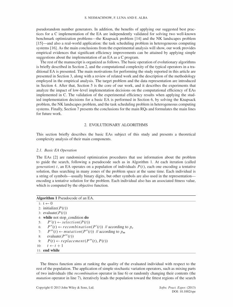
The EAs [2] are randomized optimization procedures that use information about the problemto guide the search, following a pseudocode such as in Algorithm 1. At each iteration (calledgeneration) t , an EA operates on a population of individuals P.t/, each one encoding a tentativesolution, thus searching in many zones of the problem space at the same time. Each individual isa string of symbols—usually binary digits, but other symbols are also used in the representation—encoding a tentative solution for the problem. Each individual also has an associated fitness value,which is computed by the objective function.
Algorithm 1 Pseudocode of an EA.1: t 02: initialize(P.t/)3: evaluate(P.t/)4: while not stop_condition do5: P 0.t/ selection.P.t//
6: P 00.t/ recombination.P 0.t// // according to pc7: P 000.t/ mutation.P 00.t// // according to pm8: evaluate(P 000.t/)9: P.t/ replacement.P 000.t/,P.t//
10: t t C 111: end while
The fitness function aims at ranking the quality of the evaluated individual with respect to therest of the population. The application of simple stochastic variation operators, such as mixing partsof two individuals (the recombination operator in line 6) or randomly changing their contents (themutation operator in line 7), iteratively leads the population toward the fittest regions of the search
Copyright © 2013 John Wiley & Sons, Ltd. Softw. Pract. Exper. (2013)DOI: 10.1002/spe

AN EMPIRICAL TIME ANALYSIS OF EAS AS SOFTWARE PROGRAMS
cutting point
0 0 1 0 1 1 0 1
1 1 1 1 0 0 1 0
0 0 1 0 1 0 1 0
1 1 1 1 0 1 0 1
1 1 1 1 0 0 1 0 1 1 1 1 0 1 1 0
mutation
parents offspring
Figure 2. Examples of recombination and mutation operators in an evolutionary algorithm.
space. A graphical outline of the recombination and mutation operators for binary-encoded solu-tions is provided in Figure 2. These operators are used with certain probabilities pc (the crossoverprobability for an individual) and pm (the mutation probability for each symbol in one individual),respectively. The algorithm finishes when a stopping condition is fulfilled, for example, a certainnumber of generations have been performed, an acceptable solution is found, or a given number offunction evaluations has been carried out.
Two main models exist for the evolution process presented in Algorithm 1 for an EA:
� In a generational EA, an entirely new population is generated at each iteration, which replacesthe previous one; and� In a steady-state EA, only one new individual in the population is generated at each iteration,
which replaces another selected individual to form a very similar new population.
The generational model for EAs is the one mainly used in the experimental analysis reportedhere, because both it is the canonical algorithm originally proposed in the literature and it is also themost popular one. However, the steady state model is also analyzed when the effects of the differentsorting methods for ordering the population are considered.
As to the particular operators in the EAs used for our tests in this work, we will analyze:
1. Binary tournament selection, which picks the better individual out of a set of (two) randomlyselected individuals to survive;
2. Single-point crossover (SPX), which selects a single crossover point at random and the sub-parts of the two parents between that crossover position are exchanged to create two offsprings;and
3. Bit-flip mutation, which randomly changes a given position in an individual (this operator isapplied on a bit-by-bit basis).
Because the experimental analysis mainly focuses on studying the behavior of the diverse deci-sions in the C implementation of the EA, a simple optimization problem (the OneMax problem)is addressed. However, in order to verify the computational efficiency improvements when solvinga real-world optimization problem with application in modern distributed computing systems, thetask scheduling problem in heterogeneous computing environments will be later used to show thevalidity of our conclusions.
2.2. Computational complexity of evolutionary algorithm operators
Consider an EA working with a population size P for solving an optimization problem of dimen-sion D, that is, each individual is represented by an array of dimension D (unidimensional). Thetheoretical complexity of applying each operator within the EA is presented later.
� Tournament selection complexity: best-case: O.1/, average case: O.1/, worst case: O.1/.� Crossover complexity: best case: O.1/, average case: O.D=2/, worst case: O.D/.� Mutation complexity: best case: O.D/, average case: O.D/, worst case: O.D/.
Copyright © 2013 John Wiley & Sons, Ltd. Softw. Pract. Exper. (2013)DOI: 10.1002/spe

S. NESMACHNOW, F. LUNA AND E. ALBA
� Replacement complexity (generational model): best case: O.P /, average case: O.P /, worstcase: O.P /.� Replacement complexity (steady-state model): best case: O.1/, average case: O.P=2/, worst
case: O.P /.
Thus, when using P individuals, the theoretical complexity of an EA that executes for n genera-tions is (in the worst case) O.n�P � .DCP //, that is, the EA iterates n times on a population ofP individuals, which are manipulated with operators in O.D/ (crossover and mutation) and O.P /(replacement).
It is clear that, depending on the values of P andD, the genetic operators may involve a consider-able computational effort. Indeed, in the case of the bit flip mutation operator, one random numbermust be drawn for each gene, that is, D numbers by P individuals in just one single EA iteration.Random number generation is therefore a key issue with a major impact on the EA performance,and it is one of the targets under study in the empirical analysis, which is performed later. The effectof the crossover operator is, on the other hand, mainly related to the memory management due to theexchange of portions of the tentative solutions. Finally, when tackling complex, high-dimensionaloptimization problems, it is also rather usual to set up EAs with large populations so as to providethe search with enough genetic diversity that prevents the EA to become stuck into local optima.Taking this into account, the theoretical analysis performed here has further motivated the empiricalanalysis included in this work.
3. THE IMPORTANCE OF ANALYZING THE EXECUTION TIME INEVOLUTIONARY ALGORITHMS
This section presents the main motivations for performing a time execution analysis of a C imple-mentation of EAs and a review of the related work on the influence of implementation details in theexecution time of EAs.
3.1. Motivation
Execution time is a crucial issue when facing hard-to-solve optimization problems, where an EAcan demand many hours or even days of execution. Also, in any general application, saving timecan lead to perform a higher number of independent runs per time unit, and even be an importantfactor in helping researchers to meet deadlines for conferences and more complete experimentalanalysis in journal papers. Many strategies have been proposed to reduce the execution time of EAs,such as parallel and distributed computing techniques [17], search space reduction techniques, andso on, but the implementation details targeted in this work are on a lower level.
For many optimization problems, the task which consumes the most in an EA is the fitness evalu-ation (specially, those coming from real-world scenarios). However, a non-negligible execution timehas to be devoted to the EA variation operators as well. What we mean here is that there are many fit-ness functions with low computational requirements, most of them having linear complexity, that is,O.D/ (being D the instance size), which is the same complexity as that of many standard, widelyused crossover and mutation operators (such as those used in this work: see Section 2.2). Well-known optimization problems one might consider are, for example, in combinatorial optimization,the travelling salesman problem, where the fitness function relies just on D summing up the D+1values from a distance matrix (the same holds for the vehicle routing problem, a challenging prob-lem quite relevant in the recent literature with direct application in logistics, for instance), and, innumerical optimization problem, the typical test functions (Rosenbrock, Rastrigin, etc.) that per-form real-coded operations on a D-dimensional array of floating points. Let us consider a mutationoperator that works in a gene-wise fashion (e.g., bit flip). It has to go through each gene, draw arandom number, and decide whether change update it or not. Therefore, D random numbers are tobe generated at every mutation phase, for every individual in the population, each usually involvingmany operations (shifting, masking, etc.). Under these assumptions, mutation might be computa-tional more demanding than the fitness function if the random number generator demands a highcomputational effort.
Copyright © 2013 John Wiley & Sons, Ltd. Softw. Pract. Exper. (2013)DOI: 10.1002/spe

AN EMPIRICAL TIME ANALYSIS OF EAS AS SOFTWARE PROGRAMS
Figure 3. Profiling sample for an evolutionary algorithm with linear-order fitness function.
As a relevant example, we give here a preliminary study of an EA efficiency for a linear-order fit-ness problem (Onemax).‡ When performing a profiling analysis as the one frequently performed byresearchers using the GNU gprof utility [18], we obtain the results reported in Figure 3, where theaverage execution time contributions (computed over 50 independent runs) for the different opera-tors in a classic EA are presented. The profiling shows that the mutation operator and the memorymanagement (copy of solutions) require significantly more computing time than the fitness functionevaluation. As stated earlier, the mutation operator is that heavy because it requires one randomnumber to be drawn for each gene of the individual (i.e., as many random number as the dimensionof the problem instance). This fact provides us with some hints to be further analyzed later.
Speeding up the executions means indeed that it will be possible to perform a more comprehen-sive experimental analysis of EAs (and other metaheuristics) in the same amount of research time,in this case, when using C as a programming language. For example, when solving a large numberof problem instances, where each of them requires performing many independent executions of thestudied method in order to extract numerical conclusions with statistical significance, much time isneeded. Even reductions of 10–20% could be very helpful in that situation.
The study reported in this article is aimed at providing a set of suggestions or best practices toapply when implementing EAs in C (or languages that have this set of features). The expression bestpractices refers to a set of techniques, methods, and processes that conventional wisdom regards asmore effective at delivering a particular outcome than any other technique, method, or process, whenapplied to a given particular scenario or specific circumstances. In order to compare the differentalternatives and validate the best suggestions (BS) for a C implementation of an EA, this articlewill first engage in an exhaustive empirical efficiency analysis for a wide range of the two mainparameters when solving an optimization problem (i.e., population size and problem dimension).
3.2. Related Work
Many works have studied the runtime analysis of EAs for specific optimization problems [19–22].However, the experimental evaluation of the computational efficiency of implementations for EAsand other metaheuristics in a generic sense, has seldom been studied.
Only two related works can be found in the literature about the topic of structured empiricalevaluation of execution times of EAs.
In 2007, Alba et al. [23], studied the influence of data representation in a steady-state EA imple-mented in the Java language. Different representations for the candidate solutions in Java werestudied, including a short (using byte, 8-bits), an intermediate (using integer, 32-bits), and a long(using double, 64-bits) data structure. For the EA population, the array data type and the Vector
‡It has been implemented in C, compiled with GNU gcc 4.3.2, and run on Debian 5.0. The random number generator isrand(), provided by the standard C library.
Copyright © 2013 John Wiley & Sons, Ltd. Softw. Pract. Exper. (2013)DOI: 10.1002/spe

S. NESMACHNOW, F. LUNA AND E. ALBA
class were analyzed. The experimental evaluation allowed the authors to conclude that: (i) the datastructure used for population representation significantly affects the time consumed by the Javaimplementation, and (ii) the type used for the solution representation does not have a noticeableinfluence for the studied chromosome lengths.
Recently, Merelo et al. [24] analyzed several implementation tweaks to improve the compu-tational efficiency of a module that implements EAs in the Perl scripting language. A specificmethodology for the analysis and identification of bottlenecks is presented, along with strategiesfor their elimination through several programming techniques. Instead of analyzing the effectsof the implementation details for a basic EA, techniques such as using a fitness cache or moni-tor/profiling software are studied. The main conclusions drawn from the experimental evaluationare that using a cache for fitness evaluations and applying profilers to identify the bottlenecks of EAimplementations allow improving the execution times.
Compared with the mentioned works, we here are more comprehensive in our analysis, target Cas a programming language and go for all the basic components of the EA in a structured analysis.
3.3. Methodology
In this paper, we consider the background of our personal experiences on implementing efficientEAs for solving complex problems, and some theoretical suggestions for software development thatare often left aside when implementing EAs. The main motivation of this approach is to analyzehow the decisions made in the implementation of EAs using the C programming language impact onthe computational efficiency of the developed software, to answer the five main RQs formulated inSection 1. This study is aimed at providing simple guidelines and best practices in the C implementa-tion of EAs. To make the reproducibility of this work easy, the source code used for the experimentsis publicly available to download at http://www.fing.edu.uy/inco/grupos/cecal/hpc/ETAEASP.
The experimental evaluation is designed by focusing on the implementation decisions only—static versus dynamic memory, local versus global variables, ordering the population or not, usingcode substitution mechanisms, and the pseudorandom numbers generator—, not on the specificcomponents and operators of a given EA. That is, in this article, we clearly differentiate between theabstract algorithmic structure versus the specific implementation, and we do not address particulardesign decisions—such as high level design issues in the taxonomy presented in Figure 1—in thereported experimental analysis. Hence, a standard algorithmic structure is studied to solve a simpleoptimization problem.
4. TARGET PROBLEM AND DATA REPRESENTATION
We have focused our analysis on a basic evolutionary algorithm, which follows the generic out-line presented in Algorithm 1 (Section 2). This simple EA has been implemented in C, a widelyused language to implement EAs in the literature [3, 4, 8, 25]. This section introduces the optimiza-tion problem used for the EA evaluation and the main considerations about how to implement theproblem details.
4.1. The OneMax problem
Because the goal of this work is to analyze pure implementation details of EAs, the simple OneMaxproblem has been used as a test-bed. In the OneMax problem, the goal is to maximize the numberof ones of a bitstring. Formally, given a set of binary variables Ex D Œx1, x2, : : : , xD�, xi 2 ¹0, 1º, theOneMax problem is defined by the expression in Equation 1.
maxf .Ex/DDX
iD1
xi (1)
Although the OneMax problem has a very simple formulation, it is useful to perform an empiricalanalysis focused on evaluating the computational efficiency of the EA implementation. The linearorder complexity of the fitness function used in the OneMax problem models the computational
Copyright © 2013 John Wiley & Sons, Ltd. Softw. Pract. Exper. (2013)DOI: 10.1002/spe

AN EMPIRICAL TIME ANALYSIS OF EAS AS SOFTWARE PROGRAMS
complexity of the evaluation function used in a large set of traditional combinatorial optimizationproblems, including the following:
� Routing and path planning problems, from the classical Hamiltonian cycle and TravelingSalesman Problem, to other shortest path problems and spanning tree construction problems.� Graph and set problems, including covering and partitioning, coloring, matching, clique, and
so on.� Scheduling problems, including job sequencing, multiprocessor scheduling, open-shop and
flow-shop problems.� Propositional logic problems, including the Satisfiability Problem in all its flavors.
All of the previous combinatorial optimization problems have linear order fitness functions, whichcan be expressed by the generic expression in Equation 2, where FL is a linear order function,usually related to the cost or profit of including the element xi in a solution of the problem.
min =max f .Ex/ D
DX
iD1
FL.xi / . (2)
The OneMax problem has been used in many articles as a benchmark function for evaluating thecomputational efficiency of EAs [26–29] as well as other population based metaheuristics [30].
In addition, the OneMax problem can also be used to model more complex optimization problemsinvolving constraints and other features, for example, by including exogenous noise in the fitnessevaluation as performed by Sastry et al. [31, 32].
4.2. Problem representation and memory requirements
In order for the OneMax problem to be implemented in C, we have used arrays of char, each oneusing one byte of memory. This encoding represents a trade-off between memory usage and ease ofimplementation. As a consequence, for an instance of dimension D, the total size of memory usedfor storing any given tentative solution is D bytes.
In the experiments considering the generational EA, the main data structures that have to beallocated in memory are the population, the temporary mating pool population, and the fitnessof each solution. Hence, given a population size P , the memory required for the EA to run is.2�P �D�1/C .P �8/ bytes, in which the first term corresponds to the two populations (presentand auxiliary), and the second one refers to the array of double variables for the fitness values(in C, a double value uses 8 bytes of memory). In the steady state EA, a single population with Pindividuals is used, corresponding to .P �D � 1/C .P � 8/ bytes.
Note that we have neglected, in the previous variable counts, other local auxiliary variables suchas loop indexes, because we concentrate on the components of the EA itself.
5. EXPERIMENTAL ANALYSIS
This section describes the experimental analysis devoted to study the influence of implementationdecisions on the execution time of an EA. The implementation issues that have been studied ares follows: the utilization of dynamic versus static memory, the utilization of global versus localvariables, the utilization of diverse methods for ordering the EA population when it is required, theuse of code substitution mechanisms, and the comparison among several methods for generatingpseudorandom numbers.
5.1. Methodology used in the experimental analysis
The experimental analysis has been carefully designed to properly evaluate how the previously com-mented implementation issues impact on the execution time. All the EAs have the same settings: acrossover rate of 0.6, a mutation rate of 1=D, where D is the instance dimension, and the stoppingcondition is 1, 000, 000=P , where P is the population size. A dedicated computational platform
Copyright © 2013 John Wiley & Sons, Ltd. Softw. Pract. Exper. (2013)DOI: 10.1002/spe

S. NESMACHNOW, F. LUNA AND E. ALBA
was used (i.e., the EA was the only program executing on the computer) to guarantee a precise mea-sure of the execution time, without sharing computing resources—that is, memory or CPU—withother programs. The execution time is measured with the time command line utility, retrieving theuser time.
Another main concern taken into account is the statistical validation of the time results for theevolutionary search: due to the random nature of EAs, for studying each of the implementation deci-sions considered in the experimental analysis, 50 independent executions of the proposed EA havebeen performed for a large set of problem instances combining different population sizes and prob-lem dimension values. By using the same 50 seeds for the pseudorandom numbers generation, wehave ensured that the EA implementations explore exactly the same search space, to make the samedecisions, based on the same sequence of pseudorandom numbers, except for those experimentsspecifically devoted to analyze the usage of different pseudorandom number generators.
All through this article, when comparing two EA implementations (namely, EA1 and EA2), therelative improvement, RI, of EA1 over EA2 is defined by the expression in Equation 3, wheret .EAi / is the average time (computed in the 50 executions performed for each algorithm in eachexperiment) required to execute EAi , and EA2 is supposed to be the implementation that takes thelongest execution time.
RI Dt .EA2/� t .EA1/
t.EA2/(3)
To provide the results with confidence, the following statistical procedure has been used [33].First, 50 independent runs have been performed. First a Kolmogorov–Smirnov test is performed tocheck whether the samples are distributed according to a normal distribution or not. If so, an anal-ysis of variance I test is performed; otherwise, we perform a Kruskal–Wallis test. Because morethan two algorithms are involved in the study, a post-hoc testing phase that allows for a multiplecomparison of samples has been performed. All the statistical tests are performed with a confidencelevel of 95%.
The experimental analysis is focused on the implementation of the generational model for EA,because of three main reasons: (i) it is the canonical algorithm originally proposed, (ii) it is alsowidely used in the literature, and (iii) it performs a significant larger number of operations than thesteady-state model, thus its computational efficiency is more critical. Nevertheless, the implemen-tation of the steady-state model for EA is used in those experiments devoted to analyze the effectsof the procedures for ordering the population, because a steady-state EA often requires an orderedpopulation to better handle the elitist selection and replacement criteria usually employed in theevolutionary loop.
5.2. Development and execution platform
The experimental analysis was performed on an Intel Core2 Q9400 at 2.66 GHz, with 4 GB RAMand 3 MB of cache, using Debian Linux 5.0 operating system with kernel version 2.6.26-2-686. Allthe codes were compiled with the public GNU gcc 4.3.2 compiler. This combination of operatingsystem/compiler is widely used within the EA (and metaheuristic) research community and manyissues such as memory management, might vary in other operating system/compilers, but the resultsshould be similar in other scenarios.
5.3. RQ1: dynamic versus static memory
In this first set of experiments, the goal is to compare the utilization of either static or dynamicmemory to store the main data structures of an EA, namely the population of tentative solutions andtheir corresponding fitness values. That is, the comparison has been performed between an imple-mentation using static and dynamic vectors/matrices for the fitness array values (vector) and for thetwo required populations (bi-dimensional matrices). This target has been chosen because the mem-ory requirements for these EA components usually fit within the computer memory (RAM). Also,
Copyright © 2013 John Wiley & Sons, Ltd. Softw. Pract. Exper. (2013)DOI: 10.1002/spe

AN EMPIRICAL TIME ANALYSIS OF EAS AS SOFTWARE PROGRAMS
Figure 4. Static and dynamic implementations of the main algorithm variables in an evolutionary algorithm.
Table I. Execution times of the evolutionary algorithm with static anddynamic memory.
P D M Static Dynamic ST
10 10 0.2 KB 0.41˙0.01 0.48˙0.01 +10 100 2.0 KB 3.05˙0.03 3.33˙0.05 +10 1000 19.1 KB 29.04˙0.10 32.27˙1.74 +10 10,000 195.1 KB 291.75˙5.45 324.58˙12.04 +100 10 2.7 KB 0.42˙0.02 0.49˙0.02 +100 100 20.3 KB 3.12˙0.11 3.37˙0.13 +100 1000 196.1 KB 29.49˙0.56 32.64˙1.32 +100 10000 1953.1 KB 300.55˙8.99 333.98˙11.67 +1000 10 0.02 MB 0.42˙0.06 0.49˙0.07 +1000 100 0.2 MB 3.10˙0.04 3.43˙0.15 +1000 1000 1.9 MB 29.93˙1.33 32.81˙1.02 +1000 10000 19.1 MB 329.73˙12.91 349.70˙1.60 +10000 10 0.2 MB 0.43˙0.02 0.50˙0.02 +10000 100 1.9 MB 3.20˙0.11 3.52˙0.16 +10000 1000 19.1 MB 33.17˙0.79 35.26˙1.30 +10000 10000 190.1 MB 334.31˙14.09 357.29˙6.23 +
ST: statistical test.
the amount of such memory can be rather large when large population sizes or highly dimensionaloptimization problems are used.
The two EA implementations (i.e., ‘static’ and ‘dynamic’) have the same coding, except forthe definition of the main variables in the proposed EA: fitness_var, population, andmating_pool. The differences between static and dynamic implementations are shown inFigure 4. The static version of the EA simply defines a vector (or matrix) using the adequate valuesof size_pop (population size) and dimension (dimension of the problem). On the other hand,the dynamic version uses the malloc subroutine to store the memory required for those threevariables, and the free function to free the memory, to make it available for future use.
Table I summarizes the results of the experimental analysis in which the execution times of bothEA implementations are studied. The values of the population size (P ) and problem dimension (D)determine the memory required by the EA (M ). Table I reports the averages and standard devia-tions of the execution times (in seconds) on 50 independent executions of the proposed EA for eachpopulation size and problem dimension. The last column, ST, includes the output of the statisticaltest: the ‘+’ symbols indicate that the differences are statistically different at 95% of confidencelevel. Figure 5 summarizes the RIs (in percentage) when using static versus dynamic memory forthe EA variables.
Copyright © 2013 John Wiley & Sons, Ltd. Softw. Pract. Exper. (2013)DOI: 10.1002/spe

S. NESMACHNOW, F. LUNA AND E. ALBA
Population size = 10
D=10M=0.2KB
D=100M=2.0KB
D=1000M=19.1KB
D=10000M=195KB
Population size = 100
D=10M=2.7KB
D=100M=20.3KB
D=1000M=196KB
D=10000M=1953KB
Population size = 1000
D=10M=0.02MB
D=100M=0.2MB
D=1000M=1.9MB
D=10000M=19.1MB
Population size = 10000
D=10M=0.2MB
D=100M=1.9MB
D=1000M=19.1MB
D=10000M=190.1MB
05
1015
2025
05
1015
2025
05
1015
2025
05
1015
2025
Figure 5. Execution time improvement rate of using static versus using dynamic memory for the main evo-lutionary algorithm variables when the population is 10 (top left), 100 (top right), 1000 (bottom left), and
10000 (bottom right), respectively.
The time results in Table I and the improvement values in Figure 5 demonstrate that a significantacceleration of the execution time can be obtained by using static variables to store the populationsand the fitness value array of a generational EA (with statistical confidence). This is a very importantexample of the effect in the computational efficiency of a simple implementation decision, often leftaside by researchers when implementing EAs. Using dynamic memory has been always suggestedas a good practice when programming in C/C++, as well in other high level languages, becauseallocating/deallocating blocks of memory when needed can be very useful. However, handling suchdynamic memory can be problematic and inefficient in general [34]. For many simple applications,these difficulties do not significantly affect the execution time, but for large and complex application(such as optimization problems, embedded and real time systems, . . . ), these issues should not beignored as our results show.
Our experimental analysis demonstrates that the dynamic version of the proposed EA is slower forall studied cases, due to the cost of managing the dynamic memory, which significantly slows downthe EA execution. The largest efficiency improvements are obtained when solving small dimen-sion problems (around 14%), but significant reductions in the execution times—about 10%— arealso obtained when using widely used values for the population size (i.e., 100 and 1000) for all thetackled problem dimensions.
In C, static memory is allocated using a stack-based policy, whereas dynamic memory is allo-cated from the heap using the standard library functions malloc() and free(). The simplelast-in-first-out strategy used to manage the stack is performed very efficiently and in constant time.On the other hand, the performance of allocations in the heap depends on several factors, includingthe heap complexity due to previous assignments, because the allocation requires to find a hole ofthe proper size and the deallocation requires to collapse holes to reduce fragmentation. The stack
Copyright © 2013 John Wiley & Sons, Ltd. Softw. Pract. Exper. (2013)DOI: 10.1002/spe

AN EMPIRICAL TIME ANALYSIS OF EAS AS SOFTWARE PROGRAMS
usually has a limited size, but we proved that it was able to handle up to 190 MB efficiently, althoughthe improvements tend to reduce when using more than 2 MB. A second, more subtle, reason forthe improvement of static versus dynamic populations has to do with the number of memory accessrequired to retrieve data coming from the stack or from the heap. Whereas in the first case, onlyone single access is needed (the addresses are known at compilation time), for dynamically allo-cated variables, two memory accesses are mandatory, one to obtain the pointer plus a second one toobtain the data. The experimental analysis reported in this subsection demonstrates that the differ-ences between static (stack-allocated) and dynamic (heap-allocated) memory are significant whenevaluating the execution time of an EA.
On the basis of the previous results, RQ1 can be now answered: the empirical analysis demon-strates that using a static implementation provides a significant reduction in the execution time ofthe studied EA. The average improvements in the execution times when using the static over thedynamic implementation was 9.4%, and a maximum of 14.2% was obtained for P D 10, D D 10.When efficiency is a must, a static memory allocation in C is the choice.
5.4. RQ2: global versus local variables
Another important implementation decision is the utilization of local or global variables for storingthe main data structures used within an EA. This again might seem a minor implementation detail,but the experiments will demonstrate how important it is in the computational efficiency of the Cimplementation of the considered EA, and it is also a widely used (and not recommended in anybasic programming course) practice for a fast access to these data structures. Two implementations(named ‘local’ and ‘global’) have been developed for the study. They only differ in the definitionof the fitness_var, population, and mating_pool variables, which are locally/globallydefined in the two EA implementations, respectively.
Table II reports the averages and standard deviations of the execution times (in seconds) on 50independent executions of the proposed EA using local and global variables, for each populationsize and problem dimension. The (last) ST column displays the output of the statistical analysis.
Table II clearly indicates that using local variables to store the populations and large arrays in agenerational EA allows to obtain significantly shorter execution times than using global variables(with statistical confidence in all but the larger scenario with P D 10, 000 and D D 10, 000). Thus,in addition to the bad programming practice of using global variables—which provokes undesiredlateral effects related to non-locality and also affects the legibility, modularity, and maintainabilityof the software—, here we show that the implementation using local variables is more efficient. Thegraph in Figure 6 presents the RIs of local versus global implementations on the execution time. Inpractice, gcc, as many other implementations of the C compiler, store the global variables in theheap, whereas local memory is stored in the stack. Thus, as commented in the previous subsection,the explanation to these results is that the stack provides a significantly faster memory access thanthe heap. In addition, Figure 6 also shows that the performance gains are reduced as the memory
Table II. Execution times of the evolutionary algorithm with localand global variables.
P D M Local Global ST
10 1000 19.1 KB 3.08˙0.13 3.30˙0.02 +100 100 20.3 KB 3.09˙0.01 3.41˙0.01 +100 1000 196.1 KB 29.08˙0.02 32.91˙0.46 +1000 100 199.2 KB 3.10˙0.02 3.45˙0.05 +1000 1000 1957.1 KB 29.87˙0.12 33.06˙0.67 +5000 500 2.4 MB 15.67˙0.19 16.89˙0.44 +10000 500 4.8 MB 16.26˙0.05 16.98˙0.03 +10000 1000 19.1 MB 32.96˙0.20 33.97˙0.57 +10000 10000 190.1 MB 335.29˙0.12 335.11˙1.46 �
ST: statistical test.
Copyright © 2013 John Wiley & Sons, Ltd. Softw. Pract. Exper. (2013)DOI: 10.1002/spe

S. NESMACHNOW, F. LUNA AND E. ALBA
P=10D=10M=0.2KB
P=100D=100M=20.3KB
P=100D=1000M=196.1KB
P=1000D=100M=0.2MB
P=1000D=1000M=1.9MB
P=5000D=500M=2.4MB
P=5000D=1000M=4.8MB
P=10000D=1000M=19.1MB
P=10000D=10000M=190.1MB
02
46
810
Figure 6. Execution times improvements when using local versus using global variables.
usage is higher than the cache size (3 MB). The probable reason for this behavior is that the usedprocessor (as most modern ones) implements a memory scheme that ensures the stack is alwaysheld inside the cache, to guarantee a better access speed. The compiler cannot cache the value of aglobal variable in a register, since these variables can be indirectly modified at anytime. So, the useof the cache memory is the most probable explanation for this behavior.
The preceding results provide an answer to RQ2: a significant acceleration of the executiontime, up to 11.65%, can be obtained by using local variables instead of global variables in the Cimplementation of a basic generational EA.
5.5. RQ3: ordering the population
The next series of experiments analyze two of the most popular approaches for implementingordered populations in EAs: (i) maintaining an ordered population using an ordered insertion sort(insord) function and (ii) using traditional sorting routines provided in the implementations ofthe standard C library: qsort by GNU, heapsort and mergesort by BSD. Ordered popu-lations are needed within EAs in many applications, for example, when using ranking and otherelitist strategies for selection and replacement, or when applying niche techniques to improve thepopulation diversity—such as in multimodal and multiobjective optimization problems—, amongother scenarios.
5.5.1. Ordering versus ordered insertion. The first set of experiments compares the ordered inser-tion implemented by a standard insord routine with the one implemented by using the qsortfunction provided in the standard C library. The qsort function in stdlib is an implementationof the quicksort algorithm by C.A.R. Hoare [35], which is a variant of partition-exchange sorting,in particular, the Algorithm Q by Knuth [36].
We are aware that this first set of experiments regarding ordered populations compares two sortingmethods with different algorithmic complexity. As it is stated in the complexity comparison pre-sented in Table III, quicksort is one of the fastest method for ordering unsorted lists and arrays—withO.n� logn/ complexity in the average case—,whereas the ordered insertion hasO.n2/ complexityin the average case, thus it is much less efficient on large sets than advanced sorting algorithms suchas quicksort, heapsort, or mergesort. However, insertion sort provides several advantages, includingsimple implementation and high efficiency for quite small sets, and it is efficient for data sets thatare already substantially sorted: in the best case, every insertion requires a constant time, thus n ele-ments can be inserted inO.n/ time. Furthermore, when few elements need to be included in a givenset—such as in the population when using the steady state model for EAs, for example,—insertionsort is a priori very efficient method.
Copyright © 2013 John Wiley & Sons, Ltd. Softw. Pract. Exper. (2013)DOI: 10.1002/spe

AN EMPIRICAL TIME ANALYSIS OF EAS AS SOFTWARE PROGRAMS
Table III. Algorithmic complexity for the studied sorting algorithms.
Ordering method Average-case complexity Best-case complexity Worst-case complexity
Insertion sort O.n2/ O.n/ O.n2/
Quicksort O.n� log.n// O.n� log.n// O.n2/
Mergesort O.n� log.n// O.n� log.n// O.n� log.n//Heapsort O.n� log.n// O.n� log.n// O.n� log.n//
Population size = 10 Population size = 100
Population size = 1000
D=10 D=100 D=1000 D=10000 D=10 D=100 D=1000 D=10000
D=10 D=100 D=1000 D=10000 D=10 D=100 D=1000 D=10000
−20
−15
−10
−5
05
2530
3540
8485
8687
8889
9091
98.4
98.6
98.8
99.0
99.2
99.4
Population size = 10000
Figure 7. Execution times improvements of using qsort over insertion sort with a static memoryimplementation.
Figures 7 and 8 graphically summarize the RIs on the execution time when using qsort overinsord, for static and dynamic implementations of EAs, respectively. For this set of experiments,we only provide the RIs and not the absolute average time values for each case, because the exe-cution times when using insord are several orders of magnitude larger than the execution timeswhen using qsort.
The yielded results demonstrate that the studied sorting strategies have a different behavior whenusing static and dynamic implementations for the EA. In a static implementation (Figure 7), qsortsignificantly outperforms the ordered insertion method for populations with more than 10 individ-uals. A very different situation happens for the dynamic EA implementation (Figure 8): qsortsignificantly improves over the insertion sort for populations with more than 100 individuals, butthe improvements significantly decrease when facing problems with 10,000 variables, what couldbe an unexpected result for the average EA programmer. The RIs in the execution time when usingqsort reduce from 97.5% to only 9.1% over the ordered insertion in that case.
5.5.2. Comparison of fast sorting routines . The second empirical analysis regarding ordered pop-ulations performs a comparison between the qsort function in GNU stdlib and the two sortingroutines provided by the BSD distribution: mergesort and heapsort.
Copyright © 2013 John Wiley & Sons, Ltd. Softw. Pract. Exper. (2013)DOI: 10.1002/spe

S. NESMACHNOW, F. LUNA AND E. ALBA
Population size = 10 Population size = 100
Population size = 1000
D=10 D=100 D=1000 D=10000 D=10 D=100 D=1000 D=10000
D=10 D=100 D=1000 D=10000D=10 D=100 D=1000 D=10000
−10
−5
0
05
1015
8485
8687
8889
9091
2040
6080
100
Population size = 10000
Figure 8. Execution times improvements of using qsort over insertion sort with a dynamic memoryimplementation.
An ideal sorting algorithm should have the properties of stability (equal keys are not reordered),in place operation, adaptation (speeds up to O.n/ when data is nearly sorted), and performingO.n logn/ key comparisons in the worst case and O.n/ swaps in the worst case [36]. The quicksortmethod has been often reported as faster in practice than other O.n logn/ sorting algorithms suchas mergesort and heapsort [37]. However, because there is not an ideal sorting algorithm that fulfillsall the desired properties, and because EA programmers need a guide based in numerical validation,a researcher might need to choose a proper sorting algorithm, depending on the application. Thus, itis potentially worth to perform a phase of previous empirical evaluation of sorting algorithms pre-sented in this section for EAs, before going for the actual utilization of an algorithm, to determinethe relative performance in execution time of these standard implementations.
Table IV reports the averages and standard deviations of the execution times (in seconds) on 50independent executions of the proposed EA using sort, mergesort, and heapsort, for eachpopulation size and problem dimension. The pairwise statistical comparison is included in Table V.Figures 9 and 10 summarize the RIs when using the qsort implementation in the GNU standard Clibrary with respect to the mergesort and heapsort functions in the BSD distribution on staticand dynamic memory, respectively.
The results indicate that qsort provides significant execution times improvements over the BSDmergesort and heapsort functions when using a static EA implementation, specially for the largestproblem dimension tackled. The analysis performed supports this claim because all (but just one sin-gle pairwise) comparisons are different with statistical significance. Improvements up to 20.5% inthe execution time were obtained over mergesort when using 10,000 individuals to solve a problemwith 1000 variables. The improvements over heapsort were up to 11.9%. Just like in the previ-ous set of experiments against insord, when using the dynamic EA implementation the qsortfunction was unable to maintain the high performance obtained for the static implementation and
Copyright © 2013 John Wiley & Sons, Ltd. Softw. Pract. Exper. (2013)DOI: 10.1002/spe

AN EMPIRICAL TIME ANALYSIS OF EAS AS SOFTWARE PROGRAMS
Table IV. Execution times comparison for qsort, mergesort, and heapsort.
Static Dynamic
P D qsort mergesort heapsort qsort mergesort heapsort
10 10 0.54˙0.02 0.51˙0.02 0.55˙0.01 0.58˙0.03 0.53˙0.01 0.58˙0.0110 100 3.20˙0.04 3.28˙0.17 3.37˙0.09 3.31˙0.04 3.29˙0.16 3.33˙0.1110 1000 29.55˙0.59 30.86˙2.18 31.06˙0.29 30.56˙0.48 30.74˙1.08 30.64˙1.1310 10000 294.23˙3.13 309.37˙22.73 310.42˙4.53 315.59˙3.93 308.98˙16.49 305.58˙5.03
100 10 0.61˙0.02 0.57˙0.02 0.63˙0.02 0.66˙0.02 0.60˙0.02 0.65˙0.01100 100 3.26˙0.09 3.48˙0.02 3.51˙0.03 3.41˙0.06 3.38˙0.19 3.47˙0.2100 1000 29.75˙0.69 33.00˙1.34 32.34˙2.15 30.77˙0.46 30.75˙0.55 30.9˙0.55100 10000 302.44˙3.33 338.99˙7.76 325.88˙5.1 314.6˙11.75 314.55˙11.48 314.77˙11.05
1000 10 0.67˙0.01 0.63˙0.02 0.71˙0.02 0.73˙0.02 0.62˙0.01 0.73˙0.021000 100 3.35˙0.17 3.81˙0.12 3.72˙0.14 3.56˙0.21 3.42˙0.11 3.51˙0.131000 1000 30.12˙0.13 35.63˙0.84 33.38˙1.13 31.30˙0.50 31.18˙0.44 31.76˙1.521000 10000 331.21˙8.68 394.09˙14.65 364.45˙9.51 340.07˙19.72 333.15˙3.40 333.86˙7.99
10000 10 0.75˙0.02 0.68˙0.02 0.80˙0.02 0.82˙0.01 0.67˙0.01 0.83˙0.0110000 100 3.50˙0.18 4.28˙0.21 3.97˙0.13 3.70˙0.1 3.53˙0.02 3.69˙0.1310000 1000 33.84˙0.95 42.55˙0.33 38.08˙0.64 34.41˙1.89 33.91˙0.62 34.25˙1.1810000 10000 339.24˙10.8 423.12˙4.34 384˙8.7 342.52˙12.65 343.22˙11.55 340.18˙4.63
Table V. Results of the statistical pairwise comparison for qsort, mergesort, and heapsort.
Static Dynamic
qsort qsort mergesort qsort qsort mergesortversus versus versus versus versus versus
P D mergesort heapsort heapsort mergesort heapsort heapsort
10 10 + � + + � +10 100 + + + + � +10 1000 + + + + � +10 10000 + + + + + +
100 10 + + + + � +100 100 + + + + � +100 1000 + + + + + +100 10000 + + + � + +
1000 10 + + + + � +1000 100 + + + + + +1000 1000 + + + + + +1000 10000 + + + + � �
10000 10 + + + + + +10000 100 + + + + + +10000 1000 + + + + � +10000 10000 + + + � + +
differences vanish or even reverse. Indeed, whereas the performance of qsort in the dynamic caseis a slightly worse (little longer execution times), mergesort has experienced a substantial runtimereduction. The improvement values in Figure 10 graphically displays this fact. Statistically, many ofthese differences between qsort and mergesort (and also mergesort and heapsort) are significant
Copyright © 2013 John Wiley & Sons, Ltd. Softw. Pract. Exper. (2013)DOI: 10.1002/spe
S. NESMACHNOW, F. LUNA AND E. ALBA
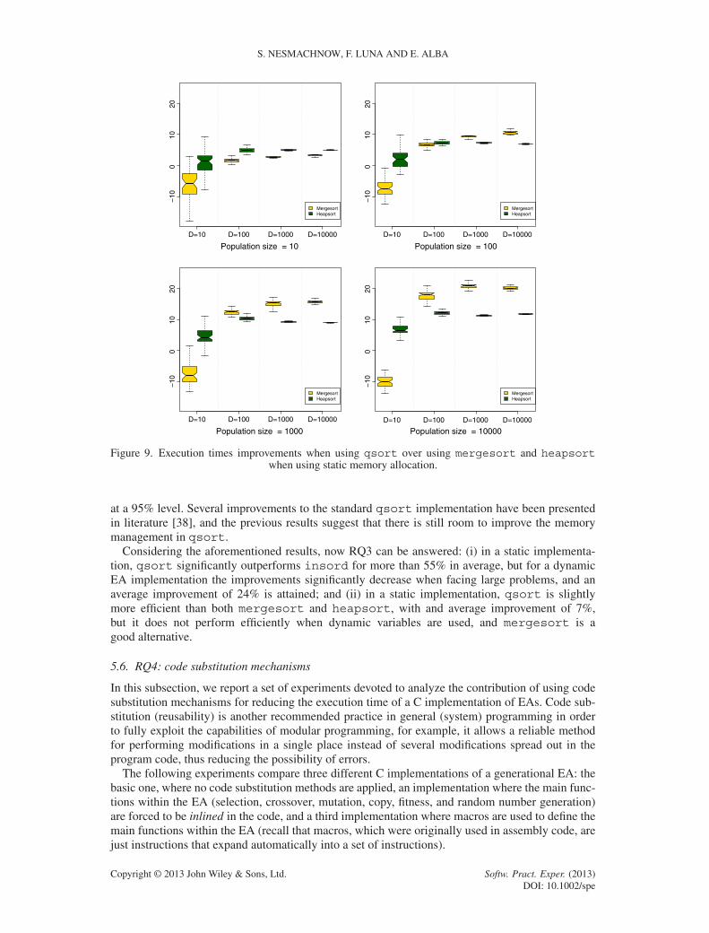
Figure 9. Execution times improvements when using qsort over using mergesort and heapsortwhen using static memory allocation.
at a 95% level. Several improvements to the standard qsort implementation have been presentedin literature [38], and the previous results suggest that there is still room to improve the memorymanagement in qsort.
Considering the aforementioned results, now RQ3 can be answered: (i) in a static implementa-tion, qsort significantly outperforms insord for more than 55% in average, but for a dynamicEA implementation the improvements significantly decrease when facing large problems, and anaverage improvement of 24% is attained; and (ii) in a static implementation, qsort is slightlymore efficient than both mergesort and heapsort, with and average improvement of 7%,but it does not perform efficiently when dynamic variables are used, and mergesort is agood alternative.
5.6. RQ4: code substitution mechanisms
In this subsection, we report a set of experiments devoted to analyze the contribution of using codesubstitution mechanisms for reducing the execution time of a C implementation of EAs. Code sub-stitution (reusability) is another recommended practice in general (system) programming in orderto fully exploit the capabilities of modular programming, for example, it allows a reliable methodfor performing modifications in a single place instead of several modifications spread out in theprogram code, thus reducing the possibility of errors.
The following experiments compare three different C implementations of a generational EA: thebasic one, where no code substitution methods are applied, an implementation where the main func-tions within the EA (selection, crossover, mutation, copy, fitness, and random number generation)are forced to be inlined in the code, and a third implementation where macros are used to define themain functions within the EA (recall that macros, which were originally used in assembly code, arejust instructions that expand automatically into a set of instructions).
Copyright © 2013 John Wiley & Sons, Ltd. Softw. Pract. Exper. (2013)DOI: 10.1002/spe

AN EMPIRICAL TIME ANALYSIS OF EAS AS SOFTWARE PROGRAMS
Figure 10. Execution times improvements when using qsort over using mergesort and heapsortwhen using dynamic memory allocation.
The use of inlined functions is often recommended to improve the performance of applications,because the compiler is requested to insert the body of the function in every place that it is called,rather than generating code to call the function, which usually demands an extra processing time toperform the lookout into the table of symbols of the program. The use of macros for code substitu-tion is a tool that allows a programmer to enable code reuse and legibility, and also provides a wayof avoiding the function call overhead.
The experimental evaluation of the execution times was performed for the static and dynamicimplementations of EAs, and using two options for compiling with gcc: full optimization withthe -O3 flag, and no optimization with the -O0 flag. We tested these two scenarios because thefull optimization flag automatically integrates all simple functions into their callers by enabling the-finline-functions option [39], thus no significant differences should be perceived in theexecution time of standard and inlined implementation when using the -O3 flag in gcc. The gccdocumentation does not clearly explain which functions are automatically inlined in such case,stating that ‘the compiler heuristically decides which functions are simple enough to be worthintegrating in this way’.
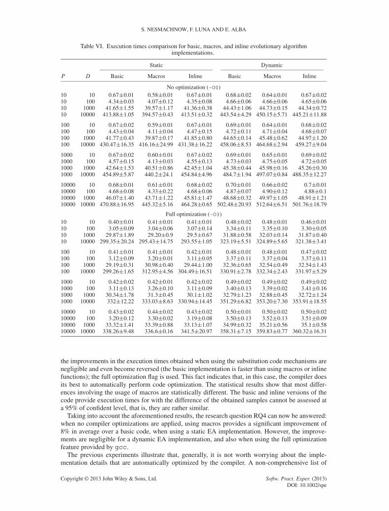
Table VI reports the averages and standard deviations of the execution times (in seconds) on 50independent executions of the proposed EA using no mechanisms for code substitution, macros, andinlined functions for each population size and problem dimension, in the two scenarios analyzed:full optimization (gcc flag -O3) and no optimization (gcc flag -O0). The statistical comparison ofthe different approaches is included in Table VII.
The results in Table VI demonstrate that when no optimization flag is employed, the use ofmacros can enhance an EA in a significant manner for the case in which a static data structure isused. The RIs are up to 15.8% for the smaller instances solved, diminishing to 3.3% for the largestinstances. For the dynamic EA implementation, the improvements were only obtained when using10 individuals in the population (typical in evolution strategies, for example). On the other hand,
Copyright © 2013 John Wiley & Sons, Ltd. Softw. Pract. Exper. (2013)DOI: 10.1002/spe
S. NESMACHNOW, F. LUNA AND E. ALBA
Table VI. Execution times comparison for basic, macros, and inline evolutionary algorithmimplementations.
Static Dynamic
P D Basic Macros Inline Basic Macros Inline
No optimization (-O0)10 10 0.67˙0.01 0.58˙0.01 0.67˙0.01 0.68˙0.02 0.64˙0.01 0.67˙0.0210 100 4.34˙0.03 4.07˙0.12 4.35˙0.08 4.66˙0.06 4.66˙0.06 4.65˙0.0610 1000 41.65˙1.55 39.57˙1.17 41.36˙0.38 44.43˙1.06 44.73˙0.15 44.34˙0.7210 10000 413.88˙1.05 394.57˙0.43 413.51˙0.32 443.54˙4.29 450.15˙5.71 445.21˙11.88
100 10 0.67˙0.02 0.59˙0.01 0.67˙0.01 0.69˙0.01 0.64˙0.01 0.68˙0.02100 100 4.43˙0.04 4.11˙0.04 4.47˙0.15 4.72˙0.11 4.71˙0.04 4.68˙0.07100 1000 41.77˙0.43 39.87˙0.17 41.85˙0.80 44.65˙0.14 45.48˙0.62 44.97˙1.20100 10000 430.47˙16.35 416.16˙24.99 431.38˙16.22 458.06˙8.53 464.68˙2.94 459.27˙9.04
1000 10 0.67˙0.02 0.60˙0.01 0.67˙0.02 0.69˙0.01 0.65˙0.01 0.69˙0.021000 100 4.57˙0.15 4.13˙0.03 4.55˙0.13 4.73˙0.03 4.75˙0.05 4.72˙0.051000 1000 42.64˙1.53 40.51˙0.86 42.45˙1.04 45.38˙0.44 45.98˙0.16 45.26˙0.301000 10000 454.89˙5.87 440.2˙24.1 454.84˙4.96 484.7˙1.94 497.07˙0.84 488.35˙12.27
10000 10 0.68˙0.01 0.61˙0.01 0.68˙0.02 0.70˙0.01 0.66˙0.02 0.7˙0.0110000 100 4.68˙0.08 4.33˙0.22 4.68˙0.06 4.87˙0.07 4.90˙0.12 4.88˙0.110000 1000 46.07˙1.40 43.71˙1.22 45.81˙1.47 48.68˙0.32 49.97˙1.05 48.91˙1.2110000 10000 470.88˙16.95 445.32˙5.16 464.28˙0.65 502.48˙20.93 512.64˙6.51 501.76˙18.79
Full optimization (-O3)10 10 0.40˙0.01 0.41˙0.01 0.41˙0.01 0.48˙0.02 0.48˙0.01 0.46˙0.0110 100 3.05˙0.09 3.04˙0.06 3.07˙0.14 3.34˙0.11 3.35˙0.10 3.30˙0.0510 1000 29.87˙1.89 29.20˙0.9 29.5˙0.67 31.88˙0.58 32.03˙0.14 31.87˙0.4010 10000 299.35˙20.24 295.43˙14.75 293.55˙1.05 323.19˙5.51 324.89˙5.65 321.38˙3.41
100 10 0.41˙0.01 0.41˙0.01 0.42˙0.01 0.48˙0.01 0.48˙0.01 0.47˙0.02100 100 3.12˙0.09 3.20˙0.01 3.11˙0.05 3.37˙0.11 3.37˙0.04 3.37˙0.11100 1000 29.19˙0.31 30.98˙0.40 29.44˙1.00 32.36˙0.65 32.54˙0.49 32.54˙1.43100 10000 299.26˙1.65 312.95˙4.56 304.49˙16.51 330.91˙2.78 332.34˙2.43 331.97˙5.29
1000 10 0.42˙0.02 0.42˙0.01 0.42˙0.02 0.49˙0.02 0.49˙0.02 0.49˙0.021000 100 3.11˙0.13 3.26˙0.10 3.11˙0.09 3.40˙0.13 3.39˙0.02 3.41˙0.161000 1000 30.34˙1.78 31.3˙0.45 30.1˙1.02 32.79˙1.23 32.88˙0.45 32.72˙1.241000 10000 332˙12.22 333.03˙8.63 330.94˙14.45 351.29˙6.82 353.20˙7.30 353.91˙18.55
10000 10 0.43˙0.02 0.44˙0.02 0.43˙0.02 0.50˙0.01 0.50˙0.02 0.50˙0.0210000 100 3.20˙0.12 3.30˙0.02 3.19˙0.08 3.50˙0.13 3.52˙0.13 3.51˙0.0910000 1000 33.32˙1.41 33.39˙0.88 33.13˙1.07 34.99˙0.32 35.21˙0.56 35.1˙0.5810000 10000 338.26˙9.48 336.6˙0.16 341.5˙20.97 358.31˙7.15 359.83˙0.77 360.32˙16.31
the improvements in the execution times obtained when using the substitution code mechanisms arenegligible and even become reversed (the basic implementation is faster than using macros or inlinefunctions); the full optimization flag is used. This fact indicates that, in this case, the compiler doesits best to automatically perform code optimization. The statistical results show that most differ-ences involving the usage of macros are statistically different. The basic and inline versions of thecode provide execution times for with the difference of the obtained samples cannot be assessed ata 95% of confident level, that is, they are rather similar.
Taking into account the aforementioned results, the research question RQ4 can now be answered:when no compiler optimizations are applied, using macros provides a significant improvement of8% in average over a basic code, when using a static EA implementation. However, the improve-ments are negligible for a dynamic EA implementation, and also when using the full optimizationfeature provided by gcc.
The previous experiments illustrate that, generally, it is not worth worrying about the imple-mentation details that are automatically optimized by the compiler. A non-comprehensive list of
Copyright © 2013 John Wiley & Sons, Ltd. Softw. Pract. Exper. (2013)DOI: 10.1002/spe

AN EMPIRICAL TIME ANALYSIS OF EAS AS SOFTWARE PROGRAMS
Table VII. Statistical significance of the results for the code substitution experiments.
Static Dynamic
-O0 -O3 -O0 -O3
Std. Std. Macros Std Std. Macros Std. Std. Macros Std. Std. Macrosversus versus versus versus versus versus versus versus versus versus versus versus
P D macros inline inline macros inline inline macros inline inline macros inline inline
10 10 + � + + � + + � + � + +10 100 + � + + � + � � � � + +10 1000 + � + + � + + � + + � +10 10000 + + + + + � + + + + � +100 10 + � + + + � + � + � + +100 100 + � + + � + + + + + � +100 1000 + � + + � + + � + + � +100 10000 + + + + + + + � + + + +1000 10 + � + � � � + � + � + �1000 100 + � + + � + + + + + � +1000 1000 + � + + � + + + + + � +1000 10000 + + + + � + + + + + + �10000 10 + � + � � � + + + � � �10000 100 + � + + � + + � + + � +10000 1000 + � + + � + + � + + � +10000 10000 + + + + � + + � + + + �
Std.: standard deviation.
other low-level issues better handled automatically by the compiler than explicitly by the pro-grammer includes: loop unrolling—because the compiler usually has privileged knowledge aboutmanaging the cache memory—, reduction of if statements and other conditional jumps—to avoidthe processor to reload the instructions queue—, optimizing branching by re-ordering instructions,and so on.
5.7. RQ5: generation of pseudorandom numbers
The last series of experiments tackles a very important implementation issue when working withnon-deterministic optimization methods: the generation of pseudorandom numbers. It is worthnoting that we are not dealing with the quality of the random number generators (for whichseveral works have been already published in the literature [11, 12]), but that we are here inter-ested in exposing any computational advantages of them from the point of view of their relativerunning time.
Two sets of experimental analyses are reported in this subsection. The first one studies theexecution times of both static and dynamic versions of the proposed EA using three methods:the two pseudorandom numbers generation functions from the standard C library—rand() anddrand48()—and an ad hoc fast multiply-with-carry (MWC) pseudorandom number generator[40], included in the comparison to analyze the time convenience of using a hand-made method forpseudorandom number generation. The second set of experiments studies the execution time of bothstatic and dynamic versions of the proposed EA when using three state-of-the-art fast pseudorandomnumbers generators: R250 [41], Mersenne Twister (MT) [42], and Tiny-MT [43].
5.7.1. Standard pseudorandom number generators. Regarding the methods for generating psudo-random numbers provided in the standard C library, it is a well-known fact that most implementa-tions of the rand() function, as many other linear congruential methods, generates pseudorandomsequences that have poor randomness properties, regarding their distribution and period [36]. How-ever, if the quality of randomness is not a special concern to solve the optimization problem, andthe user is able to estimate a priori how many pseudorandom numbers will be required for the EAexecution, implementations using simple generators as rand() have an advantage to accelerate
Copyright © 2013 John Wiley & Sons, Ltd. Softw. Pract. Exper. (2013)DOI: 10.1002/spe

S. NESMACHNOW, F. LUNA AND E. ALBA
Table VIII. Execution times (in seconds) for rand(), drand48(), and multiply-with-carry (MWC).
Static Dynamic
P D rand drand48 MWC rand drand48 MWC
100 100 3.19˙0.03 3.95˙0.29 4.65˙0.05 3.66˙0.08 4.36˙0.22 4.65˙0.02100 1000 29.14˙0.16 35.81˙2.94 43.93˙0.31 36.25˙0.03 43.21˙1.81 43.91˙0.191000 100 3.09˙0.02 3.74˙0.31 4.64˙0.02 3.38˙0.12 4.08˙0.20 4.65˙0.011000 1000 30.37˙1.91 35.87˙3.35 42.73˙0.93 32.98˙0.30 39.91˙3.06 42.71˙0.1010000 100 3.2˙0.09 3.94˙0.36 4.44˙0.27 3.59˙0.41 4.28˙0.64 4.35˙0.3210000 1000 33.16˙1.34 38.83˙2.81 44.56˙1.19 34.04˙0.77 41.36˙2.11 44.04˙0.48
Table IX. Results of the statistical pairwise comparison for rand(), drand48(), andmultiply-with-carry (MWC).
Static Dynamic
rand versus rand versus drand48 versus rand versus rand versus drand48 versusP D drand48 MWC MWC drand48 MWC MWC
100 100 C C C C C C100 1000 C C C C C C1000 100 C C C C C C1000 1000 C C C C C C10000 100 C C C C C �10000 1000 C C C C C �
the execution time. In fact, when using a standard generator such as rand() in an EA, even if theperiod is reached and the sequence of random values is repeated, they will be used for a differentpurpose in the algorithm, carrying no problems to the evolutionary search performed by the EA.This subsection studies the time efficiency of using rand(), drand48(), and MWC for a subsetof six representative problems combining population size P 2 ¹100, 1000, 10, 000º and dimensionD 2 ¹100, 1000º due to the large number of experiments required.
The quantity of pseudorandom numbers needed for solving a specific problem can be easily esti-mated by considering where are they used within the proposed EA. As an example, in the basicgenerational EA considered in this study, the quantity of pseudorandom numbers when executing ngenerations can be estimated in the following way.D�P pseudorandom numbers are needed for thepopulation initialization, whereas in each iteration the EA requires 2 � P in the selection operator,P=2C 1 to determine if a crossover operator is performed, .P=2C 1/� pC to select the crossoverpoint, andD�P in the mutation operator (i.e., for all theD alleles, it is asked whether they undergomutation or not). The total quantity of pseudorandom numbers needed is thenD�P + n� Œ.2�P +P=2C1 + .P=2C1/�pC +D�P ] =D�P.1Cn/Cn.2�P C.P=2�1/�.1CpC //. Accordingto this estimation, the quantity of pseudorandom numbers needed for the EA evaluated in this sub-section (about 1�1010 for the largest problem dimension studied) is always less than the period ofthe rand() generator (232 � 4� 1010), and obviously it is also below the periods of drand48()(248 � 2�1016) and MWC (� 4�1018), for the six problem dimensions (P �D) considered. Thus,we advice researchers to count and decide the fastest generator for their applications.
Table VIII reports the execution times in 50 independent executions of the proposed EA whenusing rand(), drand48() and MWC, for both static and dynamic implementations. The statis-tical analysis of the results is included in Table IX. The ranking is rand()/drand48()/MWC,and we report the actual improvement values. The average improvements on the execution timeswhen using the rand() generator over drand48() and MWC, for both static and dynamicimplementations, are reported in Table X.
The results in Table X indicate that significant reductions in the execution time of the studied EAsare achieved when using the standard C rand() function. The RIs were up to 19.3% with respect todrand48() and up to 33.6% with respect to MWC. The reduction in the execution times is slightlylarger for the static EA implementation than for the dynamic one. The statistical analysis support
Copyright © 2013 John Wiley & Sons, Ltd. Softw. Pract. Exper. (2013)DOI: 10.1002/spe

AN EMPIRICAL TIME ANALYSIS OF EAS AS SOFTWARE PROGRAMS
Table X. Execution time improvements when using rand() over using drand48() andmultiply-with-carry (MWC).
rand over drand48 rand over MWC
P D Static (%) Dynamic (%) Static (%) Dynamic (%)
100 100 19.27 16.05 31.48 30.01100 1000 18.61 16.11 33.60 32.151000 100 17.43 17.10 33.54 30.901000 1000 15.35 17.38 28.87 27.7510,000 100 18.80 11.09 28.03 26.5110,000 1000 14.59 17.68 25.49 24.70
Average (%) 17.34 16.92 30.16 28.67
these claims with confidence for almost all the pairwise comparisons. These results demonstrate thatthe standard rand() method is a good option for designing efficient EA implementations when thequality of the generated random numbers is not a special concern for the EA application.
5.7.2. State-of-the-art fast pseudorandom number generators. This subsection compares the exe-cution time when using three state-of-the-art fast pseudorandom numbers generators—R250, MT,and Tiny-MT—, for the two implementations of the proposed EA using static and dynamic variables.The studied generators are as follows:
� R250 [41]: a simple but efficient algorithm that implements the generalized feedback shift reg-ister method for generating pseudorandom numbers. We have used the R250 code written byM. Brundage, available in the public domain [44]. R250 is characterized by two parameters,the length (250) and the offset (103). The implementation keeps a buffer of the last 250 wordsgenerated; to generate a new word, an XOR operator is applied to the words at indexes 0 and103. The new word is added to the end of the buffer, pushing all other words down by one indexand removing the word at index zero. R250 has a huge period of almost 2250.� Mersenne Twister [42]: a generalized feedback shift register method for generation of pseudo-
random numbers. It is the most effective and popular one in the related literature among fastpseudorandom number generators. Whereas it consumes more memory than R250, MT hasbetter statistical properties and a significantly larger period of 219937 � 1.� Tiny-MT [43] is a novel small-sized variant of MT introduced in 2011. We have used the
tinymt64 implementation, which outputs 64-bit unsigned integers and double precision float-ing point numbers. Tiny-MT has far shorter period than MT, but it uses a small size of theinternal state. Thus, Tiny-MT is an usual option—that provides good statistical quality in theresulting sequences—to be used for pseudorandom numbers generation when other large stategenerators such as MT are difficult to use.
Table XI reports the average and standard deviation values of the execution times (in seconds) for50 independent executions of the proposed EA when using R250, MT, and Tiny-MT, for both staticand dynamic implementations.
Taking into account the execution times of the proposed EA using the rand() generator as areference baseline, Table XII reports the average improvements on the execution times when usingeach fast generator, for both static and dynamic implementations.
The results in Table XII show that significant reductions in an EA execution time are providedby the implementations using R250, MT, and Tiny-MT for the pseudorandom numbers generation,over the standard rand() function. The RIs were up to 64.6% for R250, up to 53.3% for MT, andup to 43.1% for Tiny-MT. The reduction in the execution times is slightly larger for the static EAimplementation.
All three pseudorandom numbers generators considered in this study have better statistical proper-ties than the standard rand() function, and they also turn to be significantly faster. R250 has goodstatistical properties and the best (lower) execution times overall. Although the execution times of
Copyright © 2013 John Wiley & Sons, Ltd. Softw. Pract. Exper. (2013)DOI: 10.1002/spe

S. NESMACHNOW, F. LUNA AND E. ALBA
Table XI. Execution times comparison for EAs using R250, Mersenne Twister (MT), and Tiny-MT.
Static Dynamic
P D R250 MT Tiny-MT R250 MT Tiny-MT
100 100 1.15˙0.01 1.54˙0.01 1.86˙0.08 1.67˙0.01 1.98˙0.16 2.22˙0.02100 1000 10.35˙0.03 13.74˙0.03 17˙0.96 16.53˙0.09 19.1˙0.14 21.91˙0.281000 100 1.16˙0.01 1.55˙0.02 1.91˙0.09 1.68˙0.01 2.02˙0.22 2.23˙0.021000 1000 10.76˙0.04 14.18˙0.03 17.27˙0.76 16.03˙0.08 18.54˙0.02 21.39˙0.2810000 100 1.24˙0.01 1.63˙0.01 1.96˙0.11 1.78˙0.02 2.08˙0.02 2.34˙0.0310000 1000 13.55˙0.06 17.02˙0.05 19.91˙0.6 18.33˙0.06 20.91˙0.08 23.79˙0.27
Table XII. Execution times improvements over rand() when using R250, Mersenne Twister (MT), andTiny-MT.
Static Dynamic
P D R250 (%) MT (%) Tiny-MT (%) R250 (%) MT (%) Tiny-MT (%)
100 100 63.9 51.8 41.7 54.3 46.0 39.3100 1000 64.5 52.9 41.7 54.4 47.3 36.91000 100 62.3 49.9 38.3 50.3 40.2 33.91000 1000 64.6 53.3 43.1 51.4 43.8 35.110000 100 61.1 49.1 59.1 50.4 42.2 34.810000 1000 59.1 48.7 40.0 46.1 38.6 30.1
Average (%) 62.6 51.0 40.6 51.1 43.0 35.5
the EA using R250 improves over MT, if quality of randomness is still a concern, MT should beused safely, because it has better statistical properties than R250, while still providing a significantefficiency improvement over the rand() generator.
We have performed here the same statistical analysis as that included up to now, but here all thedifferences are statistically significant so it does not make sense to include a new table, which infor-mation can be shown in much more little space. That is, all the previous claims are supported withstatistical confidence.
Summarizing, the answer to RQ5 is that R250 and MT are the faster pseudorandom number gen-erators, very good in numerical properties, and with notable average improvements of about 55%and 47% over rand(), respectively. MT is often found in the literature; we confirm its good runtime, and find out that R250 could even go further in time savings.
6. VALIDATION ON BENCHMARK AND REAL-WORLD SAMPLE PROBLEMS
To better illustrate the influence of the decisions made in the efficiency of C implementationof a given EA, this section studies RQ1 to RQ5, and the overall performance gains obtainedwhen solving three optimization problems: two well-known benchmark problems for combinato-rial optimization—the Knapsack problem (KP) [14] and the NK landscapes problem [15]—andalso a real-world problem—the scheduling problem in heterogeneous computing systems [16]—,by taking into account the experimental results obtained in the previous section.
The KP is a classical example of the class of constrained problems, whereas the NK problem hasbeen chosen because it most complex to evaluate, that is, the computation of the fitness functiontakes about 25% longer time than that of Onemax. The heterogeneous computing scheduling prob-lem (HCSP) has been included because it is an actual, non-academic problem, with relevance innowadays computing infrastructures.
To answer RQ1 to RQ5, a representative subset of the thorough experimentation conducted previ-ously for Onemax is presented here. The aim of this analysis is to cover a wider range of problems,thus demonstrating the usefulness and extensibility of our empirical findings on Onemax aboutimplementation decisions for EAs.
Copyright © 2013 John Wiley & Sons, Ltd. Softw. Pract. Exper. (2013)DOI: 10.1002/spe

AN EMPIRICAL TIME ANALYSIS OF EAS AS SOFTWARE PROGRAMS
Not only RQ1 to RQ5 are studied for each problem and representative instance dimensions, butwe have also compared the execution time of the implementation considering the BS from theexperimental analysis (i.e., using static memory, local variables, the qsort function, macros forcode substitution, and the MT for pseudorandom number generation) versus a raw basic implemen-tation (i.e., using dynamic memory, global variables, a mergesort function for ordering, no codesubstitution, and the drand48() function for pseudorandom number generation).
6.1. Problems definition
The mathematical formulations of the three optimization problems used in this validation part of thework are shown later, in three separated subsections.
6.1.1. Knapsack problem. The KP is a classical non-deterministic polynomial-time (NP) hardcombinatorial optimization problem [14]. Given a set of n items, each of them having associatedan integer value pi (called profit or value) and an integer value wi (known as weight), the goal ofthe KP is to find the subset of items that maximizes the total profit keeping the total weight below afixed maximum capacity (W ) of the knapsack. It is assumed that all profits and weights are positive,that all the weights are smaller than W , and that the total weight of all the items exceeds W .
The integer programming formulation of the KP is presented in Equation 4, where xi is the binarydecision variables of the problem that indicate whether the item i is included or not in the knapsack.
maximize f .Ex/DnX
iD1
pixi (4)
subject to:nX
iD1
wixi 6W
xi 2 ¹0, 1º,8i D 1, : : : ,n
In the implemented EA to solve the KP, each solution is encoded as a binary array, where thevalue in the i-th position of the array indicates if the i-th is included in the solution or not. The EAapplies a random initialization, tournament selection, SPX, and a bit-flip mutation.
6.1.2. NK landscapes. An NK landscape is a fitness function f W ¹0, 1ºN !< on binary strings,where N is the bit string length and K is the number of bits in the string that epistatically interactwith each bit (i.e., K stands for the number of other genes that epistatically affect the contributionof each gene to the overall fitness value of the string). Each gene xi , where 16 xi 6N , contributesto the total fitness of the genotype depending on the value of its allele and on those of each ofthe K other genes to which it is linked. Thus K must fall between 0 and N -1. For K D 0, thereare no interaction among genes and a single-peak landscape is obtained; in the other extreme (forK DN � 1), all genes interact each other in constructing the fitness landscape, so a completelyrandom landscape is obtained (a maximally rugged landscape). Varying K from 0 to N � 1 gives afamily of increasingly rugged multi-peaked landscapes.
The fitness value for the entire genotype is given as the average of the fitness contribution of eachlocus fi , as expressed in Equation 5, where ¹xi1 , : : : , xiK º � ¹x1, : : : , xi�1, xiC1, : : : ,N º are theKgenes interacting with gene xi in the genotype x.
f .x/D1
N
NX
iD1
fi .xi , xi1 , : : : , xiK / (5)
TheK epistatic genes could be chosen in any number of ways from the N genes in the genotype.We adopted the random neighborhoods approach [15], where the K genes are chosen at randomon the chromosome. The fitness contribution fi of xi is taken at random from a uniform distri-bution [0.0, 1.0] and depends upon its value and those present in K other genes among the N .
Copyright © 2013 John Wiley & Sons, Ltd. Softw. Pract. Exper. (2013)DOI: 10.1002/spe

S. NESMACHNOW, F. LUNA AND E. ALBA
Each gene has associated a fitness table, mapping each of the 2KC1 possible combinations of allelesto a random, real value number in the range [0,1].
In the implemented EA to solve the NK, each solution is encoded as a binary array. The EAapplies a random initialization, tournament selection, SPX, and a bit-flip mutation.
6.1.3. Heterogeneous computing scheduling. The HCSP amounts to scheduling a collection oftasks T D ¹t1, t2, : : : , tNT º (dimension NT) to be executed on a system composed by het-erogeneous machines M D ¹m1,m2, : : : ,mNM º (dimension NM). An execution time functionET W T �M ! RC defines ET .ti ,mj /, the time required to execute the task ti in the machinemj .
The goal of the HCSP is to find an assignment of tasks to machines (a function f W T N !ML),which minimizes the makespan metric, which accounts for the total time required to execute a setof tasks, as defined in Equation 6.
maxmj2M
X
ti2T W
f.ti /Dmj
ET .ti ,mj / (6)
Using the three-field notation for scheduling problems from Graham et al. [45], the HCSP is denotedRLjpij jCmax. The HCSP is a NP-hard optimization problem with direct application in nowadaysdistributed computing architectures such as clusters, grid, and cloud computing.
A simple EA was implemented to solve the HCSP, following the approach already presented bythe authors in [46]. Each solution is encoded as an array of N integers, where the value j in the i-thposition of the array indicates that task ti is scheduled to execute in machine mj . The EA applies arandom initialization, tournament selection, SPX, and a flip mutation that moves a given task froma given machine to another machine.
6.2. Experimental results
This subsection reports and analyzes the results of the experiments that studied different EA imple-mentation decision when solving the previously presented optimization problems. Three differentpopulation size for the EA has been chosen, that is, P 2 ¹100, 1000, 10, 000º, and one representativemedium-size dimension for each problem instance.
All result tables presented in the following subsections correspond to the average execution times(in seconds) and the standard deviation over 50 independent runs of the EA for each instance. Atthe end of each section of the table (one for each RQ plus the comparison of the best setting versusa raw one), the improvement reached is included, together with the results of the statistical analysis,which provides the results with confidence (ST column). A separate subsection has been used toelaborate on the results of each problem.
6.2.1. RQ1–RQ5 and best suggestions versus raw for the Knapsack problem. Table XIII displaysthe execution times and the corresponding improvements for the five RQs and the comparisonbetween the BS and the raw EA implementation for the KP. The results were computed for a rep-resentative KP instance with dimension (number of items) nD 1000 and capacity W D 1000 [47],built using the generator by Pisinger [48].
The first clear conclusion drawn from the results in Table XIII is that all the empirical findingsfor OneMax reported in Section 5 hold also in the KP problem. There are significant gains whenusing static versus a dynamic memory allocation for the EA variables (16.71% on average for thethree different values of P ) and the MT pseudorandom number generator over rand (11.69% onaverage) and drand48 (25.73% on average). A slight improvement (1.51% on average) is obtainedwhen using local versus global variables. As to the sorting methods, qsort has clearly performedbetter than both heapsort and mergesort (12.81% on average). The trend is also clear: thelarger the population, the higher the improvements, which matches with the results of OneMax. Nostatistically significant conclusions are drawn about using code substitutions strategies.
Copyright © 2013 John Wiley & Sons, Ltd. Softw. Pract. Exper. (2013)DOI: 10.1002/spe

AN EMPIRICAL TIME ANALYSIS OF EAS AS SOFTWARE PROGRAMS
Table XIII. RQ1–RQ5 results and statistical analysis when solving the Knapsack problem.
Dimension (P ,D)
RQ Implementation (100, 1000) ST (1000, 1000) ST (10,000, 1000) ST
Static 1.83˙0.05 17.64˙0.04 20.72˙0.49RQ1 Dynamic 2.44˙0.07 21.99˙0.83 21.88˙1.47
Improvement (%) 25.06 + 19.79 + 5.29 +
Local 1.82˙0.03 17.67˙0.21 20.66˙0.19RQ2 Global 1.86˙0.06 17.8˙0.47 21.03˙0.69
Improvement (%) 2.07 + 0.70 + 1.76 +
qsort 1.92˙0.01 19.55˙0.02 20.50˙0.03heapsort 2.03˙0.01 21.24˙0.03 23.47˙0.03
RQ3 mergesort 2.03˙0.01 21.87˙0.05 27.31˙0.03
Impr. qsort versus heapsort (%) 5.27 + 7.93 + 12.66 +qsort versus mergesort (%) 5.88 + 11.84 + 33.25 +
Macros 2.41˙0.01 21.87˙0.03 25.01˙0.05RQ4 No macros 2.43˙0.03 21.91˙1.12 25.13˙1.95
Improvement (%) 0.48 � 0.29 � 0.17 �
MT 1.63˙0.01 15.65˙0.03 18.62˙0.02rand 1.83˙0.02 17.80˙0.60 21.11˙2.05
RQ5 drand48 2.07˙0.27 19.50˙0.20 23.36˙3.44
Impr. MT versus rand (%) 11.17 + 12.10 + 11.80 +MT versus drand48 (%) 27.13 + 24.59 + 25.47 +
BS 1.98˙0.13 20.19˙0.04 21.13˙0.04BS versus raw Raw 2.58˙0.24 25.93˙3.12 26.05˙0.02
Improvement (%) 23.41 + 22.13 + 18.89 +
ST: statistical tests; MT: Mersenne Twister; BS: best suggestions.
The major improvements in the RQs have resulted in a major impact on the BS versus raw imple-mentation, which reaches a maximum value of 23.41% for P D 100, and 21.48% on average overthe three different settings. All the results are statistically significant.
6.2.2. RQ1-RQ5 and best suggestions versus raw for the NK. Table XIV reports the execution timesand the corresponding improvements for the five RQ and the comparison between the BS and rawimplementation for the NK problem. The results were computed for a randomly generated instanceof the NK problem, with representative dimension N D 1000 [49].
The execution times included in Table XIV are coherent with those reported for OneMax. Ofmajor relevance are the improvements of using static versus dynamic memory (up to 8.10%), ofqsort over heapsort (5.47% on average) and, specially, mergesort (9.41% on average).Regarding the pseudorandom number generators, the execution times using MT improved overrand (5.93% averaging over the three population sizes) and drand48 (12.80% on average). Nostatistically significant conclusions are drawn about using local versus global variables (0.84% inaverage) and code substitutions strategies. The main differences with respect to the OneMax resultshas to do with the slightly higher computational cost of the NK fitness computation (about 25%),which does not only require to sum up the contribution of each bit in the neighborhood but also tolook for the mapping in a fitness table.
Finally, the implementation using the BS from our experimental study and that of a raw imple-mentation shows an improvement in the execution time which between 12% and 13%. The statis-tical tests have provided most comparisons with confidence at 95% level (but those of the usingor macros).
Copyright © 2013 John Wiley & Sons, Ltd. Softw. Pract. Exper. (2013)DOI: 10.1002/spe

S. NESMACHNOW, F. LUNA AND E. ALBA
Table XIV. RQ1–RQ5 results and statistical analysis when solving the NK problem.
Dimension (P ,D)
RQ Implementation (100, 1000) ST (1000, 1000) ST (10,000, 1000) ST
Static 3.87˙0.21 38.55˙0.59 39.71˙0.07RQ1 Dynamic 4.17˙0.14 41.68˙1.53 43.22˙4.28
Improvement (%) 7.11 + 7.51 + 8.10 +
Local 3.89˙0.23 39.01˙2.80 39.78˙0.37RQ2 Global 3.90˙0.26 39.62˙4.2 40.04˙1.44
Improvement (%) 0.34 + 1.54 + 0.64 +
qsort 3.82˙0.38 37.76˙0.29 38.06˙0.06heapsort 3.88˙0.38 40.16˙0.29 41.76˙0.06
RQ3 mergesort 3.89˙0.02 40.39˙0.07 45.46˙0.05
Impr. qsort versus heapsort (%) 1.57 + 5.97 + 8.87 +
qsort versus mergesort (%) 1.84 + 6.95 + 19.45 +
Macros 4.15˙0.02 41.25˙0.02 41.02˙0.07RQ4 No macros 4.17˙0.16 41.32˙0.31 42.12˙0.52
Improvement (%) 0.48 � 0.17 � 0.24 �
MT 3.67˙0.28 36.4˙0.28 37.52˙0.06rand 3.88˙0.27 38.91˙2.17 39.83˙1.45
RQ5 drand48 4.12˙0.36 40.9˙1.96 42.61˙3.69
Impr. MT versus rand (%) 5.56 + 6.44 + 5.79 +
MT versus drand48 (%) 12.47 + 12.37 + 13.55 +
BS 3.87˙0.30 38.54˙0.20 39.17˙0.08BS versus raw raw 4.44˙0.31 44.30˙3.63 44.57˙1.28
Improvement (%) 12.79 + 12.99 + 12.12 +
Impr.: Improvement; ST: statistical tests; MT: Mersenne Twister; BS: best suggestions
6.2.3. RQ1–RQ5 and best suggestions versus raw for the heterogeneous computing schedulingproblem. For the experimental evaluation solving the HCSP, standard problem instances were gen-erated following the expected time to compute performance estimation model by Ali et al. [50]. Wechoose a representative problem dimension of 1000 tasks to execute on 10 machines, according tothe literature [16, 46]. Table XV reports the execution times and the corresponding improvementsfor the five RQ and the comparison between the BS and raw implementation for the studied EA tosolve the HCSP.
The results in Table XV demonstrate that the main conclusions drawn from the experimental anal-ysis using the OneMax function also hold for a significantly more complex optimization problemsuch as the HCSP.
The results for RQ1–RQ5 indicate the advantages of using static variables (14.98% over local, inaverage), qsort for ordering (11.20% over heapsort, in average) and the MT pseudorandom gen-erator (12.18% over rand() and 19.55% over drand48(), in average). A slight improvement of1.94% in average was obtained when using local versus global variables. No conclusive results wereobtained when analyzing the use of code substitution strategies. Furthermore, Table XV indicatesthat the average improvements on the execution times when using the BS implementation rangebetween 18.30% and 24.69%, with statistical significance.
Summary. The main conclusion of the comparative analysis for the two benchmarking problemsand real-life optimization problem addressed in this section is that a significant acceleration in the
Copyright © 2013 John Wiley & Sons, Ltd. Softw. Pract. Exper. (2013)DOI: 10.1002/spe
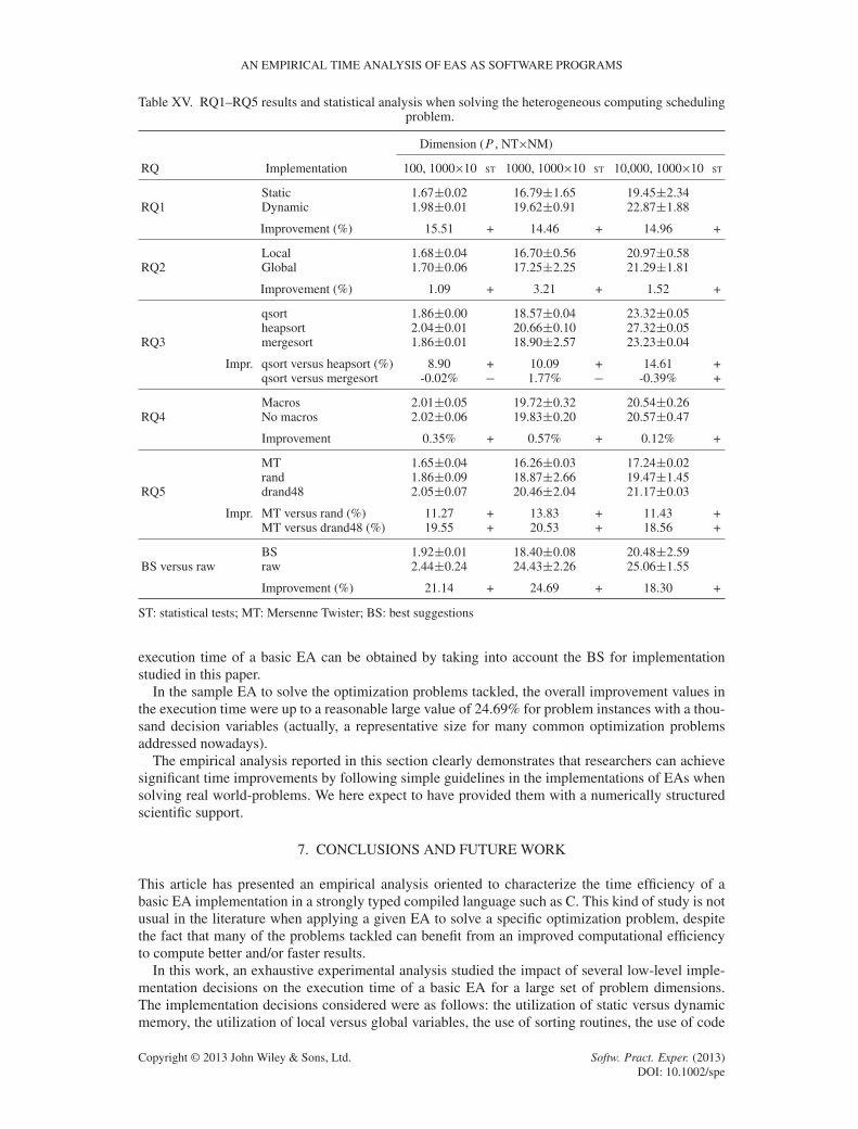
AN EMPIRICAL TIME ANALYSIS OF EAS AS SOFTWARE PROGRAMS
Table XV. RQ1–RQ5 results and statistical analysis when solving the heterogeneous computing schedulingproblem.
Dimension (P , NT�NM)
RQ Implementation 100, 1000�10 ST 1000, 1000�10 ST 10,000, 1000�10 ST
Static 1.67˙0.02 16.79˙1.65 19.45˙2.34RQ1 Dynamic 1.98˙0.01 19.62˙0.91 22.87˙1.88
Improvement (%) 15.51 + 14.46 + 14.96 +
Local 1.68˙0.04 16.70˙0.56 20.97˙0.58RQ2 Global 1.70˙0.06 17.25˙2.25 21.29˙1.81
Improvement (%) 1.09 + 3.21 + 1.52 +
qsort 1.86˙0.00 18.57˙0.04 23.32˙0.05heapsort 2.04˙0.01 20.66˙0.10 27.32˙0.05
RQ3 mergesort 1.86˙0.01 18.90˙2.57 23.23˙0.04
Impr. qsort versus heapsort (%) 8.90 + 10.09 + 14.61 +qsort versus mergesort -0.02% � 1.77% � -0.39% +
Macros 2.01˙0.05 19.72˙0.32 20.54˙0.26RQ4 No macros 2.02˙0.06 19.83˙0.20 20.57˙0.47
Improvement 0.35% + 0.57% + 0.12% +
MT 1.65˙0.04 16.26˙0.03 17.24˙0.02rand 1.86˙0.09 18.87˙2.66 19.47˙1.45
RQ5 drand48 2.05˙0.07 20.46˙2.04 21.17˙0.03
Impr. MT versus rand (%) 11.27 + 13.83 + 11.43 +MT versus drand48 (%) 19.55 + 20.53 + 18.56 +
BS 1.92˙0.01 18.40˙0.08 20.48˙2.59BS versus raw raw 2.44˙0.24 24.43˙2.26 25.06˙1.55
Improvement (%) 21.14 + 24.69 + 18.30 +
ST: statistical tests; MT: Mersenne Twister; BS: best suggestions
execution time of a basic EA can be obtained by taking into account the BS for implementationstudied in this paper.
In the sample EA to solve the optimization problems tackled, the overall improvement values inthe execution time were up to a reasonable large value of 24.69% for problem instances with a thou-sand decision variables (actually, a representative size for many common optimization problemsaddressed nowadays).
The empirical analysis reported in this section clearly demonstrates that researchers can achievesignificant time improvements by following simple guidelines in the implementations of EAs whensolving real world-problems. We here expect to have provided them with a numerically structuredscientific support.
7. CONCLUSIONS AND FUTURE WORK
This article has presented an empirical analysis oriented to characterize the time efficiency of abasic EA implementation in a strongly typed compiled language such as C. This kind of study is notusual in the literature when applying a given EA to solve a specific optimization problem, despitethe fact that many of the problems tackled can benefit from an improved computational efficiencyto compute better and/or faster results.
In this work, an exhaustive experimental analysis studied the impact of several low-level imple-mentation decisions on the execution time of a basic EA for a large set of problem dimensions.The implementation decisions considered were as follows: the utilization of static versus dynamicmemory, the utilization of local versus global variables, the use of sorting routines, the use of code
Copyright © 2013 John Wiley & Sons, Ltd. Softw. Pract. Exper. (2013)DOI: 10.1002/spe

S. NESMACHNOW, F. LUNA AND E. ALBA
substitution mechanisms, and the routines used to generate pseudorandom numbers. These decisionscan be adopted in C, but also in other C-like languages (strongly typed, compiled, able to allocatestatic/dynamic memory, etc.).
The main conclusions from the experimental analysis demonstrate that significant improvementsin the computational efficiency can be attained by applying simple suggestions when consideringthe EA as a C program that should be carefully designed and implemented. Summarizing, the exper-imental analysis showed that the improvements in the execution time were up to 10.1% when usingstatic versus dynamic memory, up to 11.7% when using local versus global variables, up to 20.5%when using the qsort routine, and up to 53.3% when using the MT pseudorandom numbers gen-erator. On the other hand, no significant improvements were detected in the comparison of codesubstitution mechanisms when using full compiler optimization capabilities.
To provide a more consistent analysis, we have conducted additional experiments with addi-tional optimization problems: two classical benchmark ones—the Knapsack problem and the NKlandscapes problem—,and a hard-to-solve optimization from real life, the scheduling problem inheterogeneous computing environments. A representative subsets of the experimental design usedto answers RQ1 to RQ5 have shown that our findings are consistent with those of OneMax, reach-ing similar improvements in the execution time. We have also shown the acceleration that can bereached by using the best implementation suggestions, which ended up from answering the five RQswith respect to a raw implementation is, averaging over three different EA population sizes: 21.48%for the KP, 12.63% for the NK problem, and 21.38% for the HCSP.
The empirical analysis allowed us to obtain very promising results when characterizing the timeefficiency of the C implementation of the EA. This allows to provide a simple list of best practicesfor developing efficient EA implementations that can be applied in many academic and industrialscenarios using C as programming language (and other C-like languages). The significant improve-ments in the execution time demonstrate that this kind of study is able to provide an immediateimpact in both those lines of research that require fast methods, such as solving very large problemscenarios and real-time optimization problems, and also in every single problem resolution that usu-ally necessitates performing a large set of independent executions to ensure the statistical quality ofthe reported results.
The main lines of research for future work include extending the computational efficiency analy-sis by considering other design and implementation decisions, and also studying different models forEAs (steady-state, distributed) with distinctive characteristics as software programs. We also planto extend and analyze particular EA implementation decisions that emerge when object-orienteddesign is used: classes, objects, inheritance, overloaded operators and functions, and so on. Inorder to show the relevance of the present work and give a first step toward the extensibility ofthe approach, we have conducted a set of preliminary experiments with g++ and Java, as the nexttargets.
First, we have used the g++ compiler (standard GNU from GNU Compiler Collection) to obtaina plain (i.e., C-like, not object oriented) implementation of the basic EA considered in our work.This allow us to argue about the similarities of using a C++ implementation. Using a medium sizeproblem dimension and population size (D D 1000 and P D 1000), the results have shown that alsosignificant improvements in the execution times are obtained when comparing static versus dynamicmemory allocation (average of 9.61% over 50 executions, with statistical significance), when usinglocal versus global variables (average of 2.62% over 50 executions, with statistical significance),and when using MT over rand/drand48 (average of 16.3% over 50 executions, with statistical sig-nificance). In addition, when studying an instance of the HCSP with 1000 tasks, 100 machines, anda population size of 100, the EA implementation using the BS was in average 25.94% faster than theraw implementation (over 50 executions, with statistical significance), also using the g++ compiler.Our claim (to be further corroborated in a future work focused on object-oriented implementations)is that low-level implementation decisions do impact in efficiency for all object-oriented languagesdesigned as extensions or supersets of C, such as C++ and Objective-C.
We have also translated the C code to Java. To avoid using object-oriented features, all the meth-ods and variables are defined as ‘static’, that is, as properties of the class. As mentioned, the analysisof these features are left for a future work. Here, the dynamic versus static implementation does
Copyright © 2013 John Wiley & Sons, Ltd. Softw. Pract. Exper. (2013)DOI: 10.1002/spe

AN EMPIRICAL TIME ANALYSIS OF EAS AS SOFTWARE PROGRAMS
not hold (in Java, all data types but primitives are dynamically allocated), so we have developedthe local versus global variables comparison. We have found that using local variables is 2.7%faster than using global variables (with statistical significance over 50 independent runs), whichis coherent with the findings in GNU gcc/g++, and also points out that this kind of low levelimplementation decisions might be also relevant in this language. We have also compared the stan-dard pseudorandom number generator in Java (class Random) with a Java implementation of MTavailable in http://www.cs.gmu.edu/~sean/research/mersenne/MersenneTwisterFast.java. Again, theresults (over 50 independent runs, with statistical significance) show that MT is 4.02% times fasterthan the standard random number generator.
The previous results suggest that the proposed line for future work is a worthy idea. Analyzingobject-oriented features shall include the evaluation of well-known object-oriented libraries such asthe Standard Template Library for C++ code.
ACKNOWLEDGEMENTS
The work of S. Nesmachnow was partly supported by Programa de Desarrollo de las Ciencias Básicas, Uni-versidad de la República, and Agencia Nacional de Investigación e Innovación, Uruguay. Francisco Lunaand Enrique Alba acknowledge partial support from the Spanish Ministry of Economy and Competitive-ness and FEDER under contracts TIN2011-28194. Francisco Luna also acknowledges partial support fromTIN2011-28336.
REFERENCES
1. Goldberg D. Genetic Algorithms in Search, Optimization, and Machine Learning. Addison Wesley: New York, 1989.2. Bäck T, Fogel D, Michalewicz Z (eds). Handbook of Evolutionary Computation. Oxford University Press: Bristol,
UK, 1997.3. Alba E, Almeida F, Blesa M, Cabeza J, Cotta C, Díaz M, Dorta I, Gabarró J, León C, Luna J, Moreno L, Pablos
C, Petit J, Rojas A, Xhafa F. MALLBA: a library of skeletons for combinatorial optimisation. Parallel Computing2006; 32(5-6):415–440.
4. Cahon S, Talbi E-G, Melab N. ParadisEO: a framework for parallel and distributed metaheuristics. Journal ofHeuristics 2004; 10(3):357–380.
5. White DR. Software review: the ECJ toolkit. Genetic Programming and Evolvable Machines 2012; 13(1):65–67.6. TIOBE Software. Tiobe programming community index, 2013. [online] http://www.tiobe.com/index.php/content/
paperinfo/tpci/index.html [last accessed March 2013].7. Grefenstette JJ. GENESIS: a system for using genetic search procedures. Proceedings of the 1984 Conference on
Intelligent Systems and Machines, Rochester, MI, USA, 1984; 161–165.8. Whitley D. The GENITOR algorithm and selection pressure: why rank-based allocation of reproductive trials is
best. In 3rd Int. Conf. on Genetic Algorithms, Schaffer JD (ed.). Morgan Kaufmann: Fairfax, Virginia, USA, 1989;116–121.
9. Nicolau M. Application of a simple binary genetic algorithm to a noiseless testbed benchmark. GECCO 2009,Montreal, Canada, 2009; 2473–2478.
10. White DR, Arcuri A, Clark JA. Evolutionary improvement of programs. IEEE Transactions on EvolutionaryComputation 2011; 15(4):515–538.
11. Cantú-Paz E. On random numbers and the performance of genetic algorithms. GECCO ’02, New York, USA, 2002;311–318.
12. Ribeiro C, Souza R, Vieira C. A comparative computational study of random number generators. Pacific Journal ofOptimization 2011; 1(3):565–578.
13. Nesmachnow S, Luna F, Alba E. Time analysis of standard evolutionary algorithms as software programs.International Conference on Intelligent Systems Design and Applications (ISDA), Córdoba, Spain, 2011; 271–276.
14. Kellerer H, Pferschy U, Pisinger D. Knapsack Problems. Springer: Berlin, Germany, 2004.15. Kauffman S, Levin S. Towards a general theory of adaptive walks on rugged landscapes. Journal of Theoretical
Biology 1987; 128(1):11–45.16. Nesmachnow S, Cancela H, Alba E. A parallel micro evolutionary algorithm for heterogeneous computing and grid
scheduling. Applied Soft Computing 2012; 12(2):626–639.17. Alba E, Luque G, Nesmachnow S. Parallel metaheuristics: recent advances and new trends. International Transac-
tions in Operational Research 2013; 20(1):1–48.18. Graham S, Kessler P, McKusick M. Gprof: a call graph execution profiler. SIGPLAN Notices 2004; 39(4):49–57.19. Laumanns M, Thiele L, Zitzler E. Running time analysis of multiobjective evolutionary algorithms on pseudo-
boolean functions. IEEE Transactions on Evolutionary Computation 2004; 8(2):170–182.20. Oliveto P, He J, Yao X. Time complexity of evolutionary algorithms for combinatorial optimization: a decade of
results. International Journal of Automation and Computing 2007; 4:281–293.
Copyright © 2013 John Wiley & Sons, Ltd. Softw. Pract. Exper. (2013)DOI: 10.1002/spe

S. NESMACHNOW, F. LUNA AND E. ALBA
21. Witt C. Runtime analysis of the (�+1) EA on simple pseudo-boolean functions. Evolutionary Computation 2006;14:65–86.
22. Zhou Y, He J. A runtime analysis of evolutionary algorithms for constrained optimization problems. IEEETransactions on Evolutionary Computation 2007; 11(5):608–619.
23. Alba E, Ferretti E, Molina J. The influence of data implementation in the performance of evolutionary algorithms.In 11th Int. Conf. on Computer Aided Systems Theory, Vol. 4739, Moreno-Díaz R, Pichler F, Quesada-Arencibia A(eds), Lecture Notes in Computer Science. Springer: Las Palmas de Gran Canaria, Spain, 2007; 764–771.
24. Merelo JJ, Romero G, Arenas M, Castillo P, Mora A, Laredo JL. Implementation matters: programming best prac-tices for evolutionary algorithms. In Advances in Computational Intelligence, Vol. 6692, Cabestany J, Rojas I, JoyaG (eds), Lecture Notes in Computer Science. Springer: Berlin/Heidelberg, 2011; 333–340.
25. Wall M. GAlib: a C++ library of genetic algorithm components. Technical report, Mechanical EngineeringDepartment, Massachusetts Institute of Technology, 1996.
26. Chen T, He J, Sun G, Chen G, Yao X. A new approach for analyzing average time complexity of population-based evolutionary algorithms on unimodal problems. Transactions on Systems, Man, and Cybernetics Part B 2009;39(5):1092–1106.
27. Johannsen D, Kurur P, Lengler J. Can quantum search accelerate evolutionary algorithms? In Proceedings of the12th annual conference on Genetic and evolutionary computation, GECCO ’10. ACM: New York, NY, USA, 2010;1433–1440.
28. Kunasol N, Suwannik W, Chongstitvatanat P. 32 solving one-million-bit problems using lzwga. Int. Symposium onInformation and Communication Technologies, Petaling Jaya, Malaysia, 2006; 32–36.
29. Lu G, Li J, Yao X. Fitness-probability cloud and a measure of problem hardness for evolutionary algorithms. In Pro-ceedings of the 11th European conference on Evolutionary computation in combinatorial optimization, EvoCOP’11.Springer-Verlag: Berlin, Heidelberg, 2011; 108–117.
30. Sudholt D. Theory of swarm intelligence. In Proceedings of the 14th international conference on Genetic andevolutionary computation companion, GECCO Companion ’12. ACM: New York, NY, USA, 2012; 1215–1238.
31. Sastry K, Goldberg D, Llora X. Towards billion-bit optimization via a parallel estimation of distribution algorithm.In Proc. of the 9th annual conference on Genetic and Evolutionary Computation, Lipson H (ed.), GECCO’07. ACM:New York, NY, USA, 2007; 577–584.
32. Suwannik W, Chongstitvatana P. Solving one-billion-bit noisy onemax problem using estimation distribution algo-rithm with arithmetic coding. Proceedings of the IEEE Congress on Evolutionary Computation, Hong Kong, China,2008; 1203–1206.
33. Sheskin DJ. Handbook of Parametric and Nonparametric Statistical Procedures. Chapman & Hall/CRC; 4 edition:Boca Raton, FL, USA, 2007.
34. Detlefs D, Dosser A, Zorn B. Memory allocation costs in large C and C++ programs. Software – Practice andExperience 1994; 24(6):527–542.
35. Hoare CAR. Quicksort. The Computer Journal 1962; 5(1):10–15.36. Knuth D. The Art of Computer Programming, Volume II: Seminumerical Algorithms. Addison-Wesley: Boston, MA,
USA, 1981.37. Skiena S. The Algorithm Design Manual (2. ed.) Springer: New York, NY, USA, 2008.38. Bentley J, McIlroy M. Engineering a sort function. Software - Practice and Experience 1993; 23(11):1249–1265.39. Loosemore S, Stallman R, McGrath R, Oram A, Drepper U. The GNU C library reference manual. Available at
http://www.gnu.org/software/libc/manual/pdf/libc.pdf [last accessed July 2013].40. Marsaglia G. Random number generators. Journal of Modern Applied Statistical Methods 2003; 2(1):2–13.41. Kirkpatrick S, Stoll E. A very fast shift-register sequence random number generator. Journal of Computational
Physics 1981; 40(2):517–526.42. Matsumoto M, Nishimura T. Mersenne twister: a 623-dimensionally equidistributed uniform pseudo-random number
generator. ACM Transactions on Modeling and Computer Simulation 1998; 8:3–30.43. Saito M, Matsumoto M. Tiny Mersenne Twister (TinyMT): a small-sized variant of Mersenne Twister, 2011.
http://www.math.sci.hiroshima-u.ac.jp/~m-mat/MT/TINYMT [last accessed January 2012].44. Brundage M. Random number generation. R250/R251, 2012. http://www.qbrundage.com/michaelb/pubs/essays/
random_number_generation.html [last accessed January 2012].45. Graham R, Lawler J, Lenstra E, Kan A. Optimization and approximation in deterministic sequencing and scheduling:
a survey. Annals of Discrete Mathematics 1979; 5:287–326.46. Nesmachnow S, Cancela H, Alba E. Heterogeneous computing scheduling with evolutionary algorithms. Soft
Computing 2010; 15(4):685–701.47. da Silva CA, Climaco J, Figueira J. A scatter search method for the bi-criteria multi-dimensional 0,1-knapsack
problem using surrogate relaxation. Journal of Mathematical Modelling and Algorithms 2004; 3:183–204.48. Pisinger D. Core problems in knapsack algorithms. Operations Research 1999; 47:570–575.49. Merz P, Freisleben B. On the effectiveness of evolutionary search in high-dimensional NK-landscapes. The 1998
IEEE International Conference on Evolutionary Computation, Anchorage, Alaska, USA, 1998; 741–745.50. Ali S, Siegel H, Maheswaran M, Ali S, Hensgen D. Task execution time modeling for heterogeneous computing
systems. Proc. of the 9th Heterogeneous Computing Workshop, Washington, DC, USA, 2000; 185–199.
Copyright © 2013 John Wiley & Sons, Ltd. Softw. Pract. Exper. (2013)DOI: 10.1002/spe