An Empirical Study of the Joint Space Inertia Matrix

Roy FeatherstoneDepartment of Systems Engineering

Australian National UniversityCanberra ACT 0200, Australia

March 6, 2004

Abstract

The joint-space inertia matrix of a robot mechanism can be highly ill-conditioned.This phenomenon is not merely a numerical artifact: it is symptomatic of an under-lying property of the mechanism itself that can make it more difficult to simulate orcontrol. This paper investigates the problem by means of an empirical study of theeigenvalues, eigenvectors and condition number of the joint-space inertia matrix. Itis shown that the condition number is typically large, and that it grows anywherefrom O(N) to O(N 4) with the number of bodies in the system. Several graphs arepresented showing how the condition number varies with configuration, the num-ber of links, variations in link sizes, variations in connectivity, and fixed or floatingbases. Explanations are offered for some of the observed effects.

1 Introduction

The joint-space inertia matrix (JSIM) plays an important role in the simulation andcontrol of robot mechanisms. It is well known that the JSIM is both symmetric andpositive-definite, but it can also be highly ill-conditioned. This property is not merely anumerical artifact: it is symptomatic of an underlying ill-conditioning phenomenon in themechanism itself. Thus, an ill-conditioned JSIM is a useful predictor of a loss of accuracyin forward and inverse dynamics calculations, even if those calculations do not involvethe JSIM directly, and it suggests that the mechanism itself may be intrinsically moredifficult to control.

This paper investigates the nature and magnitude of the ill-conditioning problem bymeans of a series of numerical experiments performed on a representative sample of robotmechanisms. These experiments show how the condition number varies as a function of:the number of links in the mechanism, the relative sizes of the links, the connectivity(characterized by a branching-factor parameter), and a fixed or a floating base. The

0This paper has been accepted for publication in the International Journal of Robotics Research, andthe final (edited, revised and typeset) version of this paper will be published in the International Journalof Robotics Research, vol. 23, no. 9, pp. 859–871, September 2004 by Sage Publications Ltd. All rightsreserved. c© Sage Publications Ltd.

1

experiments were conducted on planar, spherical, ‘circular’ and spatial mechanisms, andin a variety of configurations. However, the investigation was limited to kinematic treescontaining only revolute joints. The experiments were performed using Matlab.

The main result of this investigation is that the condition number is indeed ratherlarge, even for quite innocuous mechanisms, and that it grows asymptotically with thenumber of links anywhere from O(N) to O(N 4). For example, a planar mechanism withidentical links (as defined in Section 3) has a maximum condition number of approximately4 N4. If there are 40 links in the mechanism then the condition number can be as high as107, which would make the JSIM numerically singular in 32-bit floating-point arithmetic.If the links are not all the same size then the condition number can be substantiallyhigher still. On the other hand, branched connectivity and a floating base both tend toreduce the condition number. Even so, the results in this paper suggest that efforts tosimulate and control robotic systems with a large number of bodies will be hampered byill-conditioning to a much greater extent than might be supposed from the relatively goodresults we currently get with typical 6-DoF robots.

Much is already known about the properties of the JSIM, precisely because of its cen-tral role in many dynamics and control algorithms, but there does not appear to havebeen any previous attempt to quantify the ill-conditioning problem. Many properties ofthe JSIM were investigated by Tourassis and Neuman in [Tourassis and Neuman 1985a,Tourassis and Neuman 1985b], but not the condition number. Ghorbel, Srinivasan andSpong [Ghorbel, Srinivasan and Spong 1998] investigate the boundedness of the eigenval-ues of the JSIM, which is an essential prerequisite for the application of some controltechniques. They come up with some bounds on the largest and smallest eigenvaluefrom which an upper limit to the condition number could be deduced. Angeles and Ma[Angeles and Ma 1988] quote figures in the range 1275–1399 for the condition numberof the PUMA 600 over some example trajectories, and figures in the range 3054–11934for the Stanford Arm. They remark that these figures are large enough to cause (sig-nificant) round-off errors in calculations involving the JSIM. Ascher, Pai and Cloutier[Ascher, Pai and Cloutier 1997] consider the impact of ill-conditioning on the efficiencyof the dynamics simulation process. They show that some dynamics algorithms copebetter than others, and they suggest a modification to the articulated-body algorithm toimprove its performance on ill-conditioned systems. They also mention several examplesof robot mechanisms where ill-conditioning can be expected, including systems with longkinematic chains or large differences in link sizes. Featherstone [Featherstone 1999] plotsthe accuracy of several recursive dynamics algorithms against N . This data shows thatsome algorithms are much more accurate than others, but that they all lose accuracy as Nincreases. Both the work of Featherstone and of Ascher et al. shows that the problem lieswith the mechanism itself, since the effect is felt even by algorithms that do not calculateor use the JSIM at any stage.

This paper continues with a short review of the ill-conditioning problem, followed bya description of the robot models used in the experiments, followed by the experimentsthemselves.

2

2 Ill-Conditioning

Let A be a nonsingular matrix. The condition number of A, denoted κ(A), is a measure ofthe relative distance from A to the set of singular matrices [Golub and Van Loan 1989].(Actually, it is the reciprocal of the distance.) It therefore depends on the choice ofunderlying matrix norm. I have chosen to use the 2-norm in this paper, in which case thecondition number is defined as

κ(A) =σmax(A)

σmin(A)

where σmax(A) and σmin(A) are the largest and smallest singular values, respectively, ofthe matrix A. If A happens to be symmetric and positive-definite, like the JSIM, thenthe singular values are the same as the eigenvalues, and the condition number can begiven by the alternative definition

κ(A) =λmax(A)

λmin(A)

where λmax(A) and λmin(A) are the largest and smallest eigenvalues of A. If κ(A) islarge then A is said to be ill-conditioned.

The condition number of A defines an upper limit to the loss of precision in compu-tations involving A. Given a system described by the equation

y = Ax ,

the relative error in computing y from x is bounded by

‖δy‖‖y‖ ≤ κ(A)

‖δx‖‖x‖ ,

and the relative error in computing x from y is bounded by

‖δx‖‖x‖ ≤ κ(A−1)

‖δy‖‖y‖ = κ(A)

‖δy‖‖y‖

(since κ(A) = κ(A−1)), where δx and δy satisfy

y + δy = A (x + δx) .

The larger the value of κ(A), the greater the potential for loss of accuracy.The practical significance of ill-conditioning can be illustrated with a simple example.

Suppose we wish to command the planar robot shown in Figure 1 to accelerate from restwith a desired joint acceleration vector of

q̈d = [1, 1, 1, 1, 1, 1, 1, 1]T .

The equation of motion for this robot is

τ = H(q) q̈ + C(q, q̇)

where τ is the joint force vector, q and q̇ are the joint position and velocity vectors,H(q) is the JSIM, and C(q, q̇) is the sum of the gravity, Coriolis and centrifugal terms.

3

y

x

Figure 1: An 8-link planar robot with an ill-conditioned JSIM (actually hydra(8, 1, 0, 1)in configuration zag(π/2)).

However, as this robot moves in a horizontal plane (no gravity terms), and is initially atrest (q̇ = 0), the term C(q, q̇) simplifies to zero in this particular instance. The exactvalue of τ required to produce q̈d is therefore

τ d = Hq̈d =

302.0450 · · ·250.2104 · · ·

...8.6767 · · ·

.

If we apply exactly τ d to the robot then we will get the desired response; but what happensif we apply a slightly different force? Suppose the actuators are slightly imperfect, so thatthe actual applied force, τ a, differs very slightly from τ d. Let us say that τ a is τ d roundedto three significant figures. The robot’s response to τ a will be

q̈a = H−1τ a = H−1

30225020115110664.531.58.68

=

0.79171.02811.49040.68861.10261.09110.56261.2384

. (1)

The actual response is very different from the desired response, with errors of up to50% on individual joint axes, and yet the applied forces were all accurate to better than0.5%. High sensitivity to changes in inputs or parameters is a characteristic property ofill-conditioned systems.

In this example, the relative error was magnified by a factor of about 100; but κ(H) '1500 in the configuration shown, and there are other configurations where κ(H) > 10, 000,so the mechanism is capable of exhibiting far greater sensitivity than was evident in thisone example.

The acceleration errors lie predominantly in a subspace of joint motions that causethe least movement of the bodies in the robot mechanism. This raises the question

4

of whether this is indeed an important effect, or something that can be ignored. In asimulation context, these are the fast modes of a stiff system, and therefore cannot beignored. In a control context, the answer is less clear. It probably depends on how thecontrol system works. Any control system that uses an inverse dynamics calculation tolinearize the plant is likely to be adversely affected.

Another point to note is that the problem lies with the robot itself, not just the JSIM.Eq. 1 gives an accurate value for the acceleration response to an applied force of τ a; andthe result would not be any different if the computation were performed in a mannerthat bypassed the calculation and use of the JSIM (e.g. by using the articulated-bodyalgorithm). So it is fair to say that the mechanism itself is ill-conditioned in some sense,and that the condition number of the JSIM is a manifestation of this physical propertyrather than a purely numerical artifact.

Having put forward the idea that a rigid-body system can be ill-conditioned, it isnatural to ask what exactly this means, and how it can be quantified. Unfortunately,there is no easy answer to these questions. The obvious way to proceed is to define thecondition number of a mechanism at a specified configuration to be the ratio of the largestand smallest responses to an applied force of unit magnitude at that configuration. Theproblem with this definition is that there is no natural metric on the space of generalizedforces, and likewise no natural metric on the space of generalized accelerations. Withoutappropriate metrics, one cannot define what is meant by a unit force or the ratio of themagnitudes of two accelerations.

It is possible to proceed by defining an artificial metric. Only one metric is requiredbecause a metric defined on one space will induce a metric on the other. In the generalcase, a mechanism can contain both revolute and prismatic joints; so an artificial metricmust answer the question of how many radians of rotation shall be considered equal inmagnitude to a displacement of one metre. I have chosen to avoid this issue by excludingmechanisms containing non-revolute joints. The artificial metric used in this paper is aEuclidean metric in a system of joint coordinates such that the unit acceleration is oneradian per second per second and the unit force is one Newton-metre. (One must specifythe units as the JSIM is not invariant w.r.t. a change of units.) The final experiment inthis paper compares this metric with an inertia-weighted metric.

The main difficulty with using an artificial metric is that the eigenvalues and eigenvec-tors of the JSIM depend on the choice of metric. This is because the JSIM represents amapping from one vector space to another. The standard formula for defining eigenvaluesand eigenvectors is

Ax = λx , (2)

but this formula assumes that A is a mapping of a vector space into itself, i.e., A : U 7→ Uwhere U is a vector space. If, instead, A is a mapping from one vector space to another,e.g. A : U 7→ V , then Eq. 2 cannot be used because the LHS is an element of V , theRHS is an element of U , and the two cannot be equated. One must instead use the moregeneral formula

Ax = λBx (3)

where B is a mapping of the same kind as A. The problem with Eq. 3 is that λ and x arenow clearly functions of both A and B rather than A alone. If we use Eq. 3 to define theeigenvalues and eigenvectors of the JSIM then the value of B is determined by the choice

5

0 1 2

3

4

5

6

7

8

9

10

11

12

13

14

15

16

17fixed base (=root)

link 1

joint 1

Figure 2: A kinematic tree with a branching factor of 1.5.

of artificial metric. For the metric used in this paper, B is an identity matrix in jointcoordinates. This means we can use Eq. 2 for the numerical determination of eigenvaluesand eigenvectors.

3 Robot Models

The experiments reported in this paper were carried out using two parametric families ofrobot mechanisms. For identification purposes, one is called hydra and the other is calledonion. Both consist of tree-structured rigid-body systems with revolute joints and a fixedbase. There are four parameters altogether, and they have the same meanings in bothfamilies: N is the number of bodies, B is the branching factor, α is the angle betweensuccessive joint axes, and ρ controls the relative sizes of the links. For convenience, weuse the following notation to refer to these robots: hydra(N, B, α, ρ) means the set of allhydra robots; onion(N, 1, 0, 1) means the set of all onion robots in which B = 1, α = 0and ρ = 1; hydra(33, 1, 0, 1) refers to a specific robot; and so on.

The connectivity of a hydra or onion mechanism is defined as follows. First, the fixedbase serves as the root of the kinematic tree, and is identified as link number zero. Themoving links are then numbered consecutively from 1 to N . The connectivity is describedby a body connection array, P , such that P (i) is the link number of the parent of link i.And finally, the joints are numbered such that joint i connects from link P (i) to link i.

P is computed from the branching factor according to the formula

P (i) = b(i − 2 + dBe)/Bc ,

where the operators b· · ·c and d· · ·e round the enclosed expressions down and up, respec-tively, to the nearest integer. This formula produces a kinematic tree in which the rootnode has exactly one child, but the other nonterminal nodes have an average of B childreneach. If B = 1 then P (i) = i − 1 and the result is an unbranched kinematic chain. IfB = 2 then P = [0, 1, 1, 2, 2, . . .] and the result is a binary tree. If B is not an integerthen the nonterminal nodes alternate between bBc and dBe children in the correct ratiofor the average to be B. For example, if B = 1.5 then one half of the nonterminals haveone child and the other half have two (see Figure 2). A tree constructed according to thisformula has minimum depth for the given parameters, but is not necessarily balanced.

The skew parameter, α, is the angle between a link’s inboard and outboard joint axes,measured about the common perpendicular from the inboard axis to the outboard axis.This angle is the same for every link in the mechanism. The inboard axis is the one used

6

α

x

y

z

x =1

inboardaxis

outboardaxis

Figure 3: Link 1 of hydra(N, B, α, ρ).

by the inboard joint, which is the joint that connects the link to its parent. The outboardaxis is used by the outboard joints, if any, which connect the link to its children. The baselink is a special case: it does not have an inboard axis, and its outboard axis coincideswith the z axis of base coordinates. If a link has more than one child then it has morethan one outboard joint, but they all use the same axis. If α = 0 then every axis in themechanism is parallel.

The tapering parameter, ρ, specifies a size ratio between consecutively-numbered links:the length parameters of link i + 1 are those of link i multiplied by ρ; the mass of linki + 1 is ρ3 times that of link i; and the rotational inertia of link i + 1 is ρ5 times that oflink i. These ratios are consistent with link i + 1 being scaled geometrically with respectto link i while keeping the density constant. If ρ = 1 then every link in the mechanism isidentical.

hydra(N, B, α, ρ) is a family of spatial robots that simplify to planar robots whenα = 1. Link 1 of a hydra robot is modelled as a thin-walled cylindrical tube of length1m and radius 0.05m (see Figure 3). The tube is centred on the x axis of the link’s localcoordinate frame, and it lies between (0,0,0) and (1,0,0) in local coordinates. The inboardjoint axis coincides with the local z axis; and Link 1’s x axis coincides with the x axis ofbase coordinates when q1 = 0. The outboard joint axis passes through the point (1,0,0) inthe direction (0,− sin(α), cos(α)). The link has a mass of 1kg, a centre of mass at (0.5,0,0),and a rotational inertia about its centre of mass of diag(0.0025, 1.015/12, 1.015/12). Thekinematic and inertia properties of the other links are those of Link 1 scaled according tothe tapering formulas.

onion(N, B, α, ρ) is a family of spherical robots: every joint axis passes through asingle point at the origin of base coordinates, so every link is constrained to rotate aboutthis one point. One possible implementation of an onion robot is shown in Figure 4. Ifα = 0 then every joint axis is coincident with the z axis of base coordinates, and the linksare therefore constrained to rotate about this one axis. This kind of mechanism does notappear to have an official name, so I will call them circular mechanisms, in analogy withplanar and spherical mechanisms. The links of an onion robot are spherically symmetric:their centres of mass lie at the origin, and their rotational inertias are characterized by asingle scalar. Link 1 has a rotational inertia of 1kgm2. It is also assigned a mass of 1kg,but the link mass parameter is unimportant, as it does not affect the equation of motionof this class of robots. The inertia parameters of the other links are calculated via thetapering formulas above.

7

���������������������������������������������������������������������������������������������������������������������������������������������������������������������������������������������������������������������������������������������������������������������������������������������������������������������������������������������������������������������������������������������������������������������������������������������������������������������������������������������������������������������������������������������������������������������������������������������������������������������������������������������������������������������������������������������������������������������������������������������������������������������������������������������������������������������������������������������������������������������������������������������������������������������������������������

���������������������������������������������������������������������������������������������������������������������������������������������������������������������������������������������������������������������������������������������������������������������������������������������������������������������������������������������������������������������������������������������������������������������

���������������������������������������������������������������������������������������������������������

α z

y

��������������������������������������������������

Figure 4: A physical realization of onion(2, 1, α, ρ).

These two families were designed to give a broad coverage of several classes of mech-anism while keeping the number of parameters small. They allow us to examine spatial,planar, spherical and circular mechanisms, branched and unbranched kinematic chains,and systematic variations in link sizes and inertias.

4 Results

This section presents the results of a series of numerical experiments to investigate thecondition number, eigenvalues and eigenvectors of the JSIM of a large sample of hydraand onion robot mechanisms. The experiments were performed using Matlab.

4.1 Unbranched Planar Robots

Let us start with an investigation of how κ(H) varies with N for hydra(N, 1, 0, 1). Theseare unbranched planar robots with identical links. To conduct this investigation, weneed a means of comparing values of κ(H) for robots with different numbers of bodies.The problem is that κ(H) depends on q, so a meaningful comparison is only possibleif the robots are placed in comparable configurations. Given that we are dealing withconfigurations of hydra and onion robots, whose configuration spaces vary systematicallywith N , the following definition is appropriate: two configurations p ∈ R

m and q ∈ Rn

(m < n) are comparable if pi = qi for i = 1 . . .m and qm+1 . . . qn follow in a systematicway from p1 . . . pm. (Other definitions are possible.)

The experiments in this paper use two parameterized families of comparable configu-rations, defined as follows:

zag(θ) : qi = (−1)i+1 θ , i = 1 . . . N

andcurl(θ) : qi = θ , i = 1 . . .N .

Their names were chosen for their effect on planar hydra robots: zag(θ) puts them intoa zigzag shape, and curl(θ) winds them around a circle. Some examples are shown inFigures 5 and 1. Two robots are in comparable configurations if they are both in zag(θ)

8

x

y

(a) (b)

(c)(d) (e)

zag(0.6)

zag(2.4)

zag(3.0)

curl(0.8)

Figure 5: Examples of zag and curl configurations of hydra(N, 1, 0, 1). N = 3 in (a),N = 5 in (b,c,d) and N = 22 in (e).

configurations with the same value of θ, or are both in curl(θ) configurations with thesame value of θ. Note that zag(0) = curl(0) and zag(π) = curl(π). Note also that noneof these configurations are singular from a dynamics point of view. A configuration likezag(0) is a kinematic singularity for a hydra robot, but this singularity appears in theJacobian, not the equation of motion.

Two experiments were performed, and the results are shown in Figures 6 and 7. Thefirst experiment used zag(θ) configurations and the second used curl(θ). The curvesconnect comparable configurations at different values of N . The sample set for N consistsof the integers 1 . . . 8 followed by values from the E12 series (10, 12, 15, 18, 22, . . . ) upto 560.

Perhaps the first thing to observe is simply the magnitude of the condition number.It’s already up to 44 for a 2-DoF robot, 306 for a 3-DoF robot, and over 40,000 for a10-DoF robot. A matrix can be considered numerically singular if its condition numberis close to the resolution limit of the machine arithmetic. By this measure, the JSIM isalready potentially singular in single-precision IEEE floating-point arithmetic at N = 40.(The corresponding figure for double-precision arithmetic is N ' 6000.)

One obvious feature of the curves is that their straight sections have only two slopes.The steeper slope corresponds to a fourth-power relationship between condition numberand N , i.e., κ(H) = O(N 4), and the shallow slope corresponds to a second-power rela-tionship, κ(H) = O(N 2). An approximate formula for the worst case is κmax(H) ' 4 N4.

In Figure 6 the shallow slope is only evident at values of θ approaching π, and thereis a fairly sharp transition from the shallow slope to the steep one at a value of N thatincreases as θ gets closer to π. It turns out that the transition occurs when the zigzagshape formed by the robot covers an area that is approximately square in outline. Thishappens when N ' sec(θ/2). In the case of θ = 3.0, for example, the transition occursat N = 14. If N < 14, as in Figure 5(d), then the zigzag is wider than it is long; and ifN > 14, as in Figure 5(e), then the zigzag is longer than it is wide.

This suggests that the composite-rigid-body inertia1 of the robot as a whole is one of

1The inertia that a specified collection of rigid bodies would have if they were rigidly connected

9

100

101

102

103

100

102

104

106

108

1010

1012

θ = 0 0.6 1.6 2.4 2.8

3.0

3.1

π

Figure 6: Condition number of hydra(N, 1, 0, 1) vs. N in zag(θ) configurations for variousθ.

100

101

102

103

100

102

104

106

108

1010

1012

θ = 0

0.012

0.025 0.05 0.1 0.2 0.4

0.8

1.4

2.4 π

Figure 7: Condition number of hydra(N, 1, 0, 1) vs. N in curl(θ) configurations for variousθ.

10

the factors in the relationship between κ(H) and N . At values of N below the transition,the robot is gaining mass in linear proportion to N ; but its geometrical extent, and hencealso its radius of gyration, are dominated by the width of the zigzag, which is not varyingwith N . At values of N above the transition, the geometrical extent is dominated by thelength of the zigzag, which grows linearly with N , so the radius of gyration also growsapproximately linearly with N . Thus, the rotational inertia of the whole mechanism growsin proportion to N below the transition, and in proportion to N 3 above the transition.

This hypothesis is supported by the results in Figure 7. In this figure, the steep slopeis only evident at small values of θ, and the curves start out with the steep slope andmake a transition to the shallow slope. The transition is less sharp, and is followed by adecaying undulation before the curve settles down to the shallow slope. What’s happeninghere is that the mechanism curls into a circular arc of radius approximately 1/θ. As Nincreases, the arc progresses around the perimeter of the circle, and becomes a completecircle when N ' 2π/θ. The transition begins as the arc approaches a semicircle, and theslope reaches its first minimum when the arc has traced slightly more than one completecircle. Thus, at low values of N , the radius of gyration is growing approximately linearlywith N , but, at higher values, it reaches an upper limit determined by the radius of thecircle.

4.2 Unbranched Spatial Robots

Are the results of Section 4.1 general, or are they a special property of planar robots? Tofind out, the first experiment was repeated using the spatial robot family hydra(N, 1, 0.5, 1).These robots adopt a twisted zigzag posture in zag(θ) configurations that resembles theplanar zigzag of hydra(N, 1, 0, 1), but twisted uniformly about its central longitudinalaxis. The twisted zigzag is contained within a cylindrical volume with length and diame-ter equal to to the length and width of the corresponding planar zigzag.

Figure 8 shows the results of this experiment alongside the equivalent results forhydra(N, 1, 0, 1). As can be seen, the condition numbers of the spatial robots are slightlylower than their planar counterparts, but the overall asymptotic and transitional be-haviour is essentially the same. The condition numbers of the spatial robots are smallerby a factor of up to 2.5 on the O(N 4) curves, and only marginally smaller on the O(N 2)curve.

There are two plausible explanations for this result, but they have not been investi-gated. The first is that the cross-coupling between revolute joints is greatest when theiraxes are parallel, so one would expect the amount of cross-coupling to be less for a spatialrobot than a planar one. The second is that the twisted zigzag is slightly shorter thanthe planar zigzag when 0 < θ < π, so its rotational inertia will be slightly less when Nis above the transition. The former applies to spatial robots in general, but the latter isspecific to this experiment.

4.3 Varying the Link Sizes

Having established that the results of Section 4.1 apply to spatial robots as well as planar,the next step is to vary the link sizes. It is already known from earlier work that a large dis-

together to form a single composite rigid body [Featherstone 1987, §5.3].

11

100

101

102

103

100

102

104

106

108

1010

1012

θ = 0

1.6

2.8

3.1

π

α = 0.5 (3D)α = 0 (planar)

Figure 8: Condition number of hydra(N, 1, 0.5, 1) vs. N in zag(θ) configurations forvarious θ.

parity in link sizes can produce an ill-conditioned JSIM [Ascher, Pai and Cloutier 1997],but we will examine how link size ratios and N together affect the condition number.

The tapering parameter, ρ, allows us to construct robot mechanisms in which the linksizes follow a geometric progression: the size of link i is that of link i − 1 scaled by ρ.For any fixed value of ρ other than 1, the size ratio between the largest and smallestlinks grows exponentially with N ; so we would expect the size-ratio effect to dominateall others at sufficiently high values of N . This is borne out by the results in Figure 9.It shows the condition number of hydra(N, 1, 0, ρ) plotted against N for various valuesof ρ in configurations curl(0) and curl(π/2). The curves for ρ = 0.7 end at a size ratioof approximately 600 : 1, and the curves for ρ = 0.99 end at ratios of 28 : 1 in curl(0)and 280 : 1 in curl(π/2). The curves stop just before the JSIM goes singular (in double-precision arithmetic).

A more interesting effect is shown in Figure 10. In this experiment, the condition num-ber of hydra(N, 1, 0, ρ) was plotted against N in configurations of curl(0) and curl(π/2),exactly as in Figure 9; but, instead of a fixed tapering coefficient, there is a fixed ratiobetween the smallest and largest links in the mechanism. ρ is therefore a function of N ,and it is given by the formula

ρ =N−1√

R

where R is the ratio of smallest to largest link size.The curves are clearly exhibiting approximately the same asymptotic behaviour as

those in Figure 7. At N = 2, the condition number is dominated by the inertia ratio ofthe two links, which is R5. As N increases, the curves converge to some extent beforebecoming approximately parallel. At N = 390, which is where the data ends, the ratiosbetween the condition numbers for R = 0.1 and R = 1 are 227.5 in curl(0) and 1587

12

100

101

102

103

100

102

104

106

108

1010

1012

1014

1016

ρ = 0.7 0.90.97 0.99

1.0

1.0

θ = 0

θ = π/2

Figure 9: Condition number of hydra(N, 1, 0, ρ) vs. N at curl(0) and curl(π/2) configu-rations for various values of ρ.

100

101

102

103

100

102

104

106

108

1010

1012

1014

R = 0.1

0.2 0.4 1.0

0.1

0.2

0.4

1.0

θ = 0

θ = π/2

Figure 10: Condition number of hydra(N, 1, 0, ρ) vs. N at curl(0) and curl(π/2) config-urations for various fixed ratios of largest to smallest link. ρ = N−1

√R.

13

0 0.2 0.4 0.6 0.8 110

−2

100

102

104

106

108

1010

N = 200

50

20

8

4

2

Figure 11: Eigenvalues of hydra(N, 1, 0, 1) at zag(0), uniformly spread along the x axis,for various N .

in curl(π/2). The ratios between R = 0.1 and R = 0.2 are 8.15 in curl(0) and 15.62 incurl(π/2). These numbers are suspiciously close to the integers 8 and 16, but I have notpursued this line of inquiry.

It would be nice if we could conclude that the results of Section 4.1 apply also torobots with differing link sizes, provided the sizes vary within fixed limits. However, thedata presented so far is not sufficient to draw such a conclusion, since it relates only toa geometric progression of decreasing link sizes. Other patterns of size variation wouldhave to be investigated.

4.4 Eigenvalues and Eigenvectors

So far, we have only looked at the condition number of the JSIM, which is only a singlenumber. We can get a better picture of the JSIM, and how it varies with N and otherparameters, by examining its eigenvalues and eigenvectors.

Figure 11 shows the eigenvalues of hydra(N, 1, 0, 1) in the configuration zag(0) forvarious values of N . Each curve connects the eigenvalues for one value of N . As thereare a different number of eigenvalues in each case, they are spaced uniformly along the xaxis such that the smallest eigenvalue appears at x = 0 and the largest at x = 1. Thus,the two eigenvalues for the case N = 2 appear at x = 0 and x = 1, the four eigenvaluesfor the case N = 4 appear at x = 0, 1/3, 2/3 and 1, and so on.

We can see from this figure that the rise in condition number is due to the increasingvalue of the largest eigenvalue rather than the decreasing value of the smallest. In-deed, the smallest eigenvalue converges to a value of approximately 0.021. This value isconfiguration-dependent. In zigzag configurations, it varies between a minimum of 0.021

14

10−2

10−1

100

10−2

100

102

104

106

108

1010

N = 200

50

20

8

4

2

Figure 12: Eigenvalues of hydra(N, 1, 0, 1) at zag(0) vs. normalized period, for variousN .

at zag(0) and a maximum of 0.164 at zag(2.45). For comparison, the smallest inertiaexhibited by a single link is Imin = 0.08458, which is its rotational inertia about its centreof mass (in the x–y plane); so the smallest eigenvalue of the JSIM is actually smaller thanthe smallest inertia of a single link by about a factor of 4.

This observation is not just an empirical result. In a few simple cases, it is possi-ble to prove that the smallest eigenvalue is indeed bounded below by λmin ≥ Imin/4.hydra(N, 1, 0, 1) at zag(0) is one such case; onion(N, 1, 0, 1) in any configuration is an-other.

The curves in Figure 11 also show that most of the eigenvalues are small, and thatthe larger eigenvalues constitute an ever-smaller proportion of the total as N increases.For example, if we use the geometric mean of the smallest and largest eigenvalues as ourthreshold, then the proportion of eigenvalues above this threshold dwindles from 50% atN = 2 to 5% at N = 200.

In Figure 11, the curves appear to be converging everywhere except x = 1. This isperhaps a little misleading, since the x scale is different for each curve. Figure 12 presentsa clearer picture of how the curves evolve. It shows the same data as Figure 11, but allcurves are now plotted on a single x scale such that the ith largest eigenvalue has an xcoordinate of 1/i. Thus, the largest eigenvalue appears at x = 1, the second largest atx = 0.5, and so on. The result is a series of parallel, nearly-straight lines.

The justification for this scale is as follows. There is a close relationship between theeigenvectors of the JSIM and the vibration modes of the robot. If the eigenvectors arecalculated using the Euclidean metric then they are the same as the vibration modes thatthe robot mechanism would have if a unit-stiffness torsional spring were to be connectedacross each joint. If the links are all in a straight line (as they are in zag(0)) then the

15

0 0.1 0.2 0.3 0.4 0.5 0.6 0.7 0.8 0.9 110

−6

10−4

10−2

100

102

104

R = 1

0.4

0.2

0.1

Figure 13: Effect of tapering on eigenvalues of hydra(50, 1, 0, ρ) at curl(2.2).

vibration modes consist of a fundamental and a series of harmonics. The eigenvectorwith the largest eigenvalue is the fundamental; the eigenvector with the second largesteigenvalue is the second harmonic; and so on. Thus, the ith largest eigenvalue can beassociated with the ith harmonic, and Figure 12 plots these eigenvalues against theirnormalized period (the fundamental having a period of 1, the second harmonic a periodof 0.5, etc.).

The slope in Figure 12 indicates an approximate fourth-power relationship betweeneigenvalue magnitude and period; but the slope would necessarily be different in a con-figuration where κ(H) = O(N 2), since the value of κ(H) is determined by the endpointsof the lines.

This experiment was repeated for various zigzag configurations. The resulting curvesdiffer in scale, and exhibit some irregularities, but are otherwise broadly similar to those inFigure 11. The irregularities can be explained as a manifestation of the more complicatedvibration modes that arise in zigzag configurations.

Figure 13 shows an example of a staircase irregularity on the eigenvalue curve, and alsoshows the effect of tapering. It plots the eigenvalues of hydra(50, 1, 0, ρ) in curl(2.2) forvarious end-link size ratios (i.e., ρ = 49

√R) on the same x scale as for Figure 11. There is

nothing special about this configuration: it was chosen simply because it produces a clearexample of a staircase. It just so happens that the condition number of hydra(50, 1, 0, 1)is quite low in curl(2.2). However, despite the large difference in scale and the super-imposed staircase pattern, the curves for hydra(50, 1, 0, 1) in Figures 13 and 11 do haveapproximately the same overall shape.

The effect of tapering is to alter the slope of the left and central portions of the curve.It also smooths out the irregularities to some extent. The smallest eigenvalue decreasesin proportion to the inertia of the smallest link (i.e., in proportion to R5); and the largest

16

0 2 4 6 8 10 12 14 16 18 20−0.4

−0.3

−0.2

−0.1

0

0.1

0.2

0.3

0.4

0.5

0.6

e1

e2

e3

d1

Figure 14: Largest eigenvectors of hydra(20, 1, 0, 1) and hydra(10, 1, 0, 1) at zag(0).

x

y

Figure 15: hydra(10, 1, 0, 1) and hydra(20, 1, 0, 1) in configurations of 0.2 times theirlargest eigenvectors.

eigenvalue decreases slightly faster than the composite inertia of the whole mechanism(i.e., slightly faster than H11). Asymptotically, the former dominates. These resultsprovide part of the explanation for the effects seen in Figure 10.

Now let us look at some eigenvectors. Figure 14 shows the three largest eigenvectorsof hydra(20, 1, 0, 1) (e1, e2 and e3) and the largest eigenvector of hydra(10, 1, 0, 1) (d1),all plotted in joint coordinates (i.e., the ith circle on each curve is the joint-i coordinate ofthe eigenvector). e2 and e3 have been included only to illustrate the connection betweeneigenvalues and vibration modes.

Figure 14 provides us with an explanation of why, in Figures 6 and 7, the conditionnumber grows faster by one power of N than the composite inertia of the whole mech-anism. Observe that the coordinates of d1 and e1 are all positive. This means thatthe corresponding joint motions sum along the length of the mechanism. The effect isillustrated in Figure 15, which shows hydra(10, 1, 0, 1) in the configuration 0.2d1 and

17

hydra(20, 1, 0, 1) in 0.2 e1, the two robots being scaled to appear the same size. Observethat hydra(20, 1, 0, 1) has curved more than hydra(10, 1, 0, 1), despite the fact that bothvectors have the same Euclidean magnitude. This is because

∑

20

i=1 e1i >∑

10

i=1 d1i eventhough

∑

20i=1 e2

1i =∑

10i=1 d2

1i = 1. In fact, one can show that the sum of the elements ofthe largest eigenvector grow in proportion to

√N .

The effect is like having a gear box with a gear ratio of√

N interposed between jointspace and the mechanism itself: if the actual inertia is growing in proportion to N x thenthe apparent inertia in joint space is growing in proportion to N x+1, being the actualgrowth multiplied by the square of the gear ratio. As there is no gearing effect on thesmallest eigenvalue, the net effect on the condition number is that it too grows by onepower of N faster than the composite inertia of the mechanism.

For the mechanisms we have studied so far, the following formula accurately predictsthe asymptotic behaviour of κ(H), but not its magnitude:

κ(H) = O(N H11/HNN) .

Essentially, it says that the asymptotic behaviour is the product of the gearing effect andthe ratio of the largest and smallest inertias in the system. (It assumes that Link N isthe smallest link in the mechanism.)

4.5 Branching Factor

Let us now examine the condition number of branched kinematic chains. We shall useonion robots, rather than hydra, on the grounds that altering the branching factor ofa hydra robot causes a large change in its shape, and hence its mass distribution. Incontrast, the links of an onion robot are all spherically symmetric and centred at theorigin; so this family of robots allows us to study the effects of varying the branchingfactor while keeping the mass distribution constant.

Figure 16 shows how the condition number of onion(N, B, 0, 1) varies with N for var-ious values of B. These are circular robots, because the skew angle is set to zero, whichmeans that the condition number is independent of configuration. The curve correspond-ing to B = 1 has a slope that is O(N 2), which is consistent with earlier results: for thisclass of mechanisms, the composite rigid-body inertia of the whole mechanism grows inproportion to N , so the condition number grows in proportion to N 2.

Branching factors greater than 1 produce curves that follow the B = 1 curve upto the point where the first branch occurs, and then make a gradual transition to anapproximately O(N) slope. The curves bottom out at B = 2; i.e., the curves for B > 2all follow approximately the same path as for B = 2. (This was checked up to B = 4.)

This experiment was repeated with onion(N, B, 1, 1), in order to discover whether theresults in Figure 16 apply to spherical robots in general, or are just a special property ofcircular robots. The curves for onion(N, B, 1, 1) are lower in magnitude and slightly moreirregular in shape than those for onion(N, B, 0, 1); but they follow the same pattern asthe curves in Figure 16, except that they bottom out at B = 3 instead of B = 2.

An explanation for these results can be found in Figure 17. This figure shows the joint-space coordinates of the largest eigenvectors of onion(33, 1, 0, 1) and onion(33, 1.125, 0, 1).The latter has branch points at links 8, 16 and 24; so the first eight joints all lie on acommon stem, the next eight lie alternately on one or other of two subtrees, the next

18

100

101

102

103

100

101

102

103

104

105

106

B = 1

1.025

1.1

1.333

2

Figure 16: Condition number of onion(N, B, 0, 1) vs. N at curl(0) for various values ofB.

0 5 10 15 20 25 30 350

0.05

0.1

0.15

0.2

0.25

0.3

0.35

B = 1

B = 1.125

Figure 17: Largest eigenvectors of onion(33, B, 0, 1) for B = 1 and B = 1.125.

19

nine each lie on one of three subtrees, and the final eight each lie on one of four subtrees.The individual joint coordinates are clearly weighted according to the number of linkssupported by the joint: motion is concentrated into the joints that move the largestnumber of links. The concentration becomes more pronounced as B increases.

Branching diminishes, and eventually eliminates, the gearing effect for two reasons.The first is that the gearing effect depends on the summation of motion that occurs whenjoints are connected in series. In an unbranched chain, all N joints are connected in series.In a branched chain, the determining factor is the maximum number of joints betweenany link and the base, which is, of course, given by the depth of the tree. With hydra andonion robots, the depth of the tree grows in proportion to log(N) when B > 1. The secondreason is that the gearing effect is largest when a large proportion of the joints contributealmost equally to the motion, and is smallest when a small number of joints account formost of the motion; so the gearing effect is reduced when the motion is concentrated intothe joints nearest the root.

4.6 Floating Bases

A floating-base robot is one that does not have a permanent kinematic connection to afixed location in space. Examples include humanoids, space robots, and mobile robots ingeneral. This category includes many robots with relatively large values of N , so it makessense to examine the effect of a floating base on the condition number of the JSIM.

The method used here is to compare the condition number of a floating-base robot withits fixed-base equivalent. The latter is obtained from the former by attaching the floatingbase to a fixed location. A special function was written to convert a fixed-base hydra robotto a floating-base robot by removing the first joint. Starting with hydra(N, B, α, ρ), thisfunction produces a robot with N bodies but only N − 1 joints. Its fixed-base equivalentis therefore the robot hydra(N−1, B, α, ρ). (There is a scale error in this comparison ifρ 6= 1, but the condition number is independent of scale.)

Figure 18 compares κ(H) for fixed-base and floating-base hydra(N, 1, 0, 1) in variouszigzag configurations. It shows that the condition number behaves in essentially the samemanner for a floating-base robot as for a fixed-base robot, but is somewhat smaller inmagnitude. In this particular experiment, the floating-base condition number is a factorof 4 lower on the O(N 2) slopes, a factor of 40 lower on the O(N 4) slopes, and the transitionoccurs at a value of N approximately a factor of 3 larger than for the fixed-base case.

In general, a floating base will reduce the largest eigenvalue of the JSIM. This will usu-ally lead to a smaller condition number, but not always. Figure 19 compares the largesteigenvectors of fixed-base hydra(10, 1, 0, 1) and floating-base hydra(11, 1, 0, 1). Observethat the latter involves much less movement of mass. This will be true in general, sincethe overall centre of mass remains stationary in a floating-base system. (The applicationof external forces is a separate issue.) In this particular example, the floating-base eigen-vector produces a symmetrical bend, each half of which resembles the fixed-base bend ofa robot with half as many joints. The situation would, of course, be different if the robotwere tapered or branched.

Despite the reduction in the largest eigenvalue, it is possible for a floating-base robotto have a larger condition number than its fixed-base equivalent. This happens whenthe floating-base link plays an important role in determining the smallest eigenvalue.

20

100

101

102

103

100

102

104

106

108

1010

1012

θ = 0

1.2

3.05

π

0

1.2

3.05

π

floating base

fixed base

Figure 18: Condition number of floating-base hydra(N+1, 1, 0, 1) compared with fixed-base hydra(N, 1, 0, 1) in zag(θ) configurations.

x

y

Figure 19: Fixed-base hydra(10, 1, 0, 1) and floating-base hydra(11, 1, 0, 1) in configura-tions of 0.2 times their largest eigenvectors.

21

To take an extreme example, consider floating-base hydra(3, 1, 0, 10) in zag(π/2). Thefloating base in this mechanism is the smallest link by a factor of 10, and it determinesthe magnitude of the smallest eigenvalue. The condition number of this mechanism is105; but the condition number of its fixed-base equivalent is only 136, mainly because ofa large increase in the smallest eigenvalue.

4.7 Changing the Metric

All of the results so far have been obtained using a Euclidean metric. One obvious criticismof this approach is that the Euclidean metric treats all joints equally. This is difficult tojustify when one considers that some joints have a much larger effect than others onthe motion of the mechanism. This section repeats some of the earlier experiments, andcompares the results obtained using the Euclidean metric with those obtained using aninertia-weighted metric.

Suppose we define a new unit of rotational measure individually for each joint, so thatrotation about joint i is measured in units of di × radians, where di is a scaling factor. Itis then necessary to adjust the units of joint force so that a unit force about joint i is 1/di

Newton-metres. This adjustment preserves the correct relationship between generalizedmotion coordinates and generalized force coordinates. If q̈, τ and H represent a jointacceleration vector, a joint force vector and a JSIM in the original coordinates, and q̈′, τ ′

and H′ represent the same quantities in the new coordinates, then

q̈′ = D−1 q̈ , τ′ = D τ

andH′ = DHD ,

whereD = diag(d1, d2, . . . , dN)

(a diagonal matrix). If we choose di according to the formula

di = H−0.5ii

then the diagonal elements of H′ are all unity. Thus, D is the coordinate transformationmatrix that scales the units of measurement in joint space such that each joint sees a unitinertia. The Euclidean metric in this scaled coordinate system is equivalent to an inertia-weighted metric in the original coordinates; so, if we define κ′(H) to be the conditionnumber of H according to the inertia-weighted metric, then

κ′(H) = κ(H′) = κ(DHD) .

Figure 20 shows both κ(H) and κ′(H) for hydra(N, 1, 0, 1) in zag(θ) configurationsfor various values of θ. Overall, the two metrics produce very nearly the same results.The inertia-weighted metric produces slightly smaller condition numbers at low values ofN and slightly larger condition numbers at large values of N .

This is an interesting result because it demonstrates that the well-known large differ-ences in magnitude between the largest and smallest diagonal elements of H are not the

22

100

101

102

103

100

102

104

106

108

1010

1012

θ = 0

1.6

2.8

3.1

π

scaled

unscaled

Figure 20: Condition number of hydra(N, 1, 0, 1) according to both the inertia-weightedand Euclidean metrics, in zag(θ) configurations for various θ.

100

101

102

103

100

102

104

106

108

1010

1012

1014

1016

ρ = 0.9

0.97 0.99

1.0

0.99

0.97

0.9

scaled

unscaled

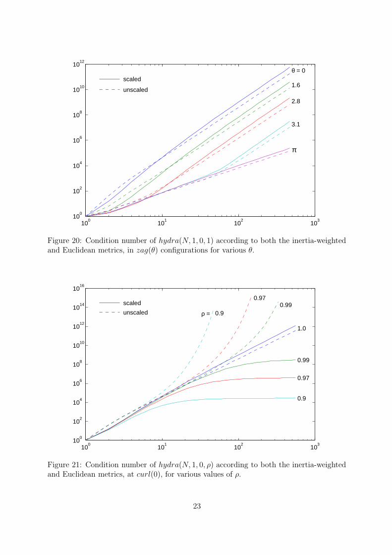
Figure 21: Condition number of hydra(N, 1, 0, ρ) according to both the inertia-weightedand Euclidean metrics, at curl(0), for various values of ρ.

23

cause of the ill-conditioning problem: if one scales the matrix to make all the diagonalelements the same then the condition number goes up, not down, for large N .

Figure 21 shows κ(H) and κ′(H) for hydra(N, 1, 0, ρ) in curl(0) for various values of ρ.The two metrics are now clearly producing very different results: for ρ < 1, κ(H) growsexponentially with N , while κ′(H) converges to a limit that depends on ρ.

There is not enough data here to draw any firm conclusions, but it does suggest thefollowing physically-plausible hypothesis: The ill-conditioning of the underlying mechan-ical system is caused largely by dynamic interactions between the bodies; the effect isstrongest when the bodies have similar inertias; and it diminishes to zero as the inertiadifferences grow. This would imply that κ′ is providing a reasonable indication of theunderlying ill-conditioning when ρ < 1, while κ is providing an overestimate.

Additional support for this hypothesis comes from examining the elements of H′. Forexample, for hydra(5, 1, 0, ρ) in curl(0), we have

H′ =

1 0.984 0.929 0.822 0.6250.984 1 0.974 0.884 0.6870.929 0.974 1 0.952 0.7690.822 0.884 0.952 1 0.8830.625 0.687 0.769 0.883 1

when ρ = 1, and

H′ =

1 0.594 0.252 0.097 0.0340.594 1 0.593 0.251 0.0920.252 0.593 1 0.590 0.2380.097 0.251 0.590 1 0.5590.034 0.092 0.238 0.559 1

when ρ = 0.5. The off-diagonal elements H ′

ij measure the dynamic interaction betweenbodies i and j. These values are all lower when ρ = 0.5, and their magnitudes diminish asthe size difference between bodies i and j increases. H′ converges to the identity matrixas ρ → 0.

5 Conclusion

This paper has presented an empirical study of the condition number of the joint-spaceinertia matrix (JSIM), backed up with some investigation of the eigenvalues and eigen-vectors of the JSIM. The study was restricted to two families of robots in which all thejoints were revolute; but it included examples of planar, spatial, spherical and ‘circular’robots, systematic variations in relative link sizes, branched and unbranched chains, andboth fixed and floating bases. Condition numbers were calculated using two families ofcomparable configurations: one in which all the joint angles were the same, and one inwhich they alternated in sign.

The general conclusion one can draw from this study is that the condition numbercan be very large, and it can grow asymptotically with the fourth power of the number ofbodies in the system. For a simple planar chain of identical links, the maximum conditionnumber is approximately 4 N 4, where N is the number of bodies. Thus, a chain of only10 links already can exhibit a condition number of 40,000.

24

If the link sizes vary, then the condition number of the JSIM goes up as the sizedifferences increase; but if the JSIM is first scaled to have unit elements along the diagonal,then the condition number of this scaled matrix goes down as the size differences increase.Branches in the kinematic chain can reduce the growth in the condition number by up toone power of N compared with an unbranched chain. A floating base can make mattersworse, but typically yields a modest reduction in condition number that does not appearto grow with N .

The significance of these results is that ill-conditioned systems are both harder tosimulate accurately and harder to control. Although a typical 6-DoF robot arm can besimulated and controlled perfectly adequately, this does not mean that the same wouldnecessarily be true of a larger system, since the condition number grows so rapidly withN . This is not just a problem with the JSIM: it is a physical property of the robotmechanism, and will therefore have an effect even on simulators and control systems thatdo not use the JSIM.

And finally, all the results in this paper depend on an arbitrary choice of metric. Onlytwo metrics were investigated: a Euclidean metric in a configuration space of revolutejoint angles, and an inertia-weighted version of the Euclidean metric. A different choiceof metric may well produce different results.

References

[Angeles and Ma 1988]Angeles, J. and Ma, O. 1988. Dynamic Simulation of n-Axis Serial Robotic Manip-ulators Using a Natural Orthogonal Complement. Int. J. Robotics Research, vol. 7,no. 5, pp. 32–47.

[Ascher, Pai and Cloutier 1997]Ascher, U. M., Pai, D. K., and Cloutier, B. P. 1997. Forward Dynamics, EliminationMethods, and Formulation Stiffness in Robot Simulation. Int. J. Robotics Research,vol. 16, no. 6, pp. 749–758.

[Featherstone 1987]Featherstone, R. 1987. Robot Dynamics Algorithms. Boston: Kluwer Academic Pub-lishers.

[Featherstone 1999]Featherstone, R. 1999. A Divide-and-Conquer Articulated-Body Algorithm for Par-allel O(log(n)) Calculation of Rigid-Body Dynamics. Part 2: Trees, Loops and Ac-curacy. Int. J. Robotics Research, vol. 18, no. 9, pp. 876–892.

[Ghorbel, Srinivasan and Spong 1998]Ghorbel, F., Srinivasan, B., and Spong, M. W. 1998. On the Uniform Boundednessof the Inertia Matrix of Serial Robot Manipulators. J. Robotic Systems, vol. 15, no.1, pp. 17–28.

[Golub and Van Loan 1989]Golub, G. H., and Van Loan, C. F. 1989. Matrix Computations. Baltimore: TheJohns Hopkins University Press.

25

[Tourassis and Neuman 1985a]Tourassis, V. D., and Neuman, C. P. 1985. Properties and Structure of DynamicRobot Models for Control Engineering Applications. Mechanism & Machine Theory,vol. 20, no. 1, pp. 27–40.

[Tourassis and Neuman 1985b]Tourassis, V. D., and Neuman, C. P. 1985. The Inertial Characteristics of DynamicRobot Models. Mechanism & Machine Theory, vol. 20, no. 1, pp. 41–52.

26