Embed Size (px)
Citation preview

An Empirical Examination of Conditional Four-Moment
CAPM and APT Pre-Specified Macroeconomic Variables
with Market Liquidity in Arab Stocks Markets
By
Ali Abubaker Ali
Thesis Submitted to the University of Gloucestershire for the
Degree of Doctor of Philosophy in Accounting and Finance
July 2011

I
Abstract
This thesis empirically examined conditional four-moment CAPM and APT pre-specified
macroeconomic variables with market liquidity in four Arab stock markets, namely Jordan,
Morocco, Tunisia and Kuwait over a period extended from January 1998 to December 2009.
The desire to test these models in the Arab stock market was motivated by that fact that
stock returns in these markets do not follow normal distribution and there exist third and
fourth moments (skewness and kurtosis). More than 50% of the realised returns from the
Arab stock market are lower than the risk free return, meaning the realised return is
negative. Arab countries are different in terms of their economic situation and many have
carried out economic reform programmes. In addition, their stock markets have been
affected by multiple political and economic shocks. Arab stock markets are characterised by
a low number of listed companies, low trading volume, low value of market capitalisation,
and hence low market liquidity.
Examination of the conditional four-moment CAPM was performed using panel data
regression, whereas APT pre-specified macroeconomic variables with market liquidity by
using six macroeconomic variables: industrial production, inflation, money supply, interest
rate, exchange rate and oil price, panel data regression and Principal Components Analysis
(PCA).
The results of unconditional two-, three- and four-moment CAPM showed that there was not
a significant positive relationship between beta and co-kurtosis, and return and that there
was an insignificant relationship between co-skewness and return which was opposite to
sign of market skewness in all stock markets included in the sample. However, the results of
testing conditional two-, three- and four-moment CAPM showed a significant positive
(negative) relationship between beta and return in an up (down) market in all the stock
markets included in the sample. The results of conditional three- and four-moment CAPM
showed a significant negative (positive) relationship between co-skewness and return when
the market was up (down) in Jordan and Tunisia. Based on the results of conditional four-
moment CAPM, a positive (negative) relationship between co-kurtosis and return in up
(down) markets was found in Tunisia only when using a value weighted index (VWI).
The results of panel data regression and PCA revealed that the most important
macroeconomic variables that remain significant in explaining stock returns were oil price for
Jordan and exchange rate and oil price for Kuwait. With respect to market liquidity, the
results showed a significant negative relationship between market liquidity and stock returns
in both Jordan and Kuwait. Generally, empirical results showed that the most important variable to explain the cross-section of stock returns is conditional co-variance (conditional beta), whereas the importance of others variables (co-skewness, co-kurtosis, macroeconomic variables and market liquidity) were different from market to other.

II
Dedication
To the memory of my brother Sahell

III
ACKNOWLEDGEMENT
All thanks to Allah who helped me to complete this thesis. I would like to take this opportunity
to express my sincere gratitude to Dr Jasim Al-Ali and Dr Bob Greenwood for their guidance,
advice, encouragement, wonderful support and valuable comments during the period of my
study. I would also like to thank my family for their patience and support during the four
years I spent completing my PhD.

IV
List of Contents
Chapter 1 Introduction .................................................................................................................................... 1
1.1 Background .................................................................................................................................................. 1
1.1.1 Conditional four-moment CAPM. ......................................................................................................... 2
1.1.2 APT pre-specified macroeconomic variables ........................................................................................ 9
1.1.3 Market liquidity ................................................................................................................................... 11
1.2 Research motivations ................................................................................................................................. 13
1.3 Research questions: .................................................................................................................................... 15
1.4 Research objectives and contributions: ...................................................................................................... 16
1.5 Structure of the research: ........................................................................................................................... 17
Chapter 2 Conditional Four-Moment CAPM ................................................................................................... 19
2.1 Introduction ................................................................................................................................................ 19
2.2 Theory of unconditional two-moment CAPM ............................................................................................. 22
2.2.1 Derivation of unconditional two-moment CAPM ............................................................................... 22
2.2.1.1 Capital market line (CML) ............................................................................................................ 24
2.2.1.2 Security market line (SML) .......................................................................................................... 30
2.2.2 Empirical tests of unconditional two-moment CAPM ........................................................................ 32
2.2.2.1 The impact of other variables ...................................................................................................... 48
2.2.2.2 Roll’s critique ............................................................................................................................... 51
2.3 Theory of unconditional four-moment CAPM ............................................................................................ 56
2.3.1 Derivation of unconditional four-moment CAPM ............................................................................... 56
2.3.2 Empirical tests of unconditional four-moment CAPM ........................................................................ 61
2.3.2.1 Empirical tests of unconditional three-moment CAPM ............................................................... 62
2.3.2.2 Empirical tests of unconditional four-moment CAPM ................................................................. 67
2.4 Theory of conditional two-moment CAPM ................................................................................................. 73
2.4.1 Derivation of conditional two-moment CAPM. .................................................................................. 74
2.4.1.1 Heterogenous beliefs................................................................................................................... 74
2.4.1.2 The market portfolio ................................................................................................................... 76
2.4.1.3 Risk-free asset borrowing and lending ........................................................................................ 78
2.4.2 Empirical tests of conditional two-moment CAPM. ............................................................................ 81
2.5 Theory of conditional four-moment CAPM ................................................................................................. 89
2.5.1 Derivation of conditional four-moment CAPM ................................................................................... 90
2.5.2 Empirical tests of conditional four-moment CAPM ............................................................................ 91
2.6 Summary .................................................................................................................................................... 96
Chapter 3 APT Pre-Specified Macroeconomic Variables with Market Liquidity ........................................... 100
3.1 Introduction .............................................................................................................................................. 100
3.2. Theory of APT .......................................................................................................................................... 105
3.3 Determination of risk factors of APT ........................................................................................................ 109
3.3.1 Statistical approach ........................................................................................................................... 109
3.3.1.1 Factor analysis ........................................................................................................................... 109
3.3.1.2 Principal component analysis .................................................................................................... 110

V
3.3.2 Macroeconomic variables approach ................................................................................................. 112
3.3.2.1 Industrial production ................................................................................................................. 114
3.3.2.2 Interest rate ............................................................................................................................... 115
3.3.2.3 Money supply ............................................................................................................................ 116
3.3.2.4 Inflation ..................................................................................................................................... 117
3.3.2.5 Exchange rate ............................................................................................................................ 117
3.3.2.6 Oil prices .................................................................................................................................... 118
3.4 Empirical tests of relationship between macroeconomic variables and stock return .............................. 120
3.4.1 Empirical tests using time series approach ....................................................................................... 120
3.4.2 Empirical tests using APT macroeconomic approach ....................................................................... 131
3.5 Market liquidity ........................................................................................................................................ 150
3.5.1 Nature of market liquidity ................................................................................................................ 150
3.5.2 Empirical tests of market liquidity .................................................................................................... 155
3.6 Summary .................................................................................................................................................. 164
Chapter 4 Research Methodology ................................................................................................................ 168
4.1 Introduction .............................................................................................................................................. 168
4.2 Research philosophy and approach .......................................................................................................... 170
4.2.1 Research philosophy ......................................................................................................................... 170
4.2.2 Research approach ........................................................................................................................... 171
4.3 Research method ................................................................................................................................. 176
4.3.1 Sample and data collection of testing conditional four-moment CAPM .......................................... 176
4.3.1.1 Sample ....................................................................................................................................... 176
4.3.1.2 Data sources .............................................................................................................................. 179
4.3.2 Analysis techniques and procedures used to test conditional four-moment CAPM. ....................... 181
4.3.2.1 Analysis techniques ................................................................................................................... 181
4.3.2.2 Testing procedures .................................................................................................................... 188
4.3.2.3 Hypotheses of testing conditional four-moment CAPM ........................................................... 193
4.3.3 Data collection and testing method of APT pre-specified macroeconomic variables. ..................... 197
4.3.3.1 Data sources .............................................................................................................................. 197
4.3.3.2 Testing procedures using panel data regression. ...................................................................... 201
4.3.3.3 Hypotheses of testing APT pre-specified macroeconomic variables. ........................................ 201
4.3.3.4 Testing procedures using Principal Components Analysis (PCA) ............................................... 202
4.3.4 Data collection and analysis testing method of market liquidity ...................................................... 203
4.3.4.1 Data sources .............................................................................................................................. 203
4.3.4.2 Testing procedures .................................................................................................................... 204
4.4 Summary .................................................................................................................................................. 206
Chapter 5 Empirical Results of Testing Conditional Four- Moment CAPM .................................................... 209
5.1 Introduction .............................................................................................................................................. 209
5.2 Empirical results of testing unconditional four-moment CAPM ............................................................... 211
5.2.1 The results of existence of skewness and kurtosis in stock returns ................................................. 211
5.2.2 Summary statistics of variables......................................................................................................... 213
5.2.3 The results of testing unconditional two-moment CAPM ................................................................ 216
5.2.4 The results of testing unsystematic risk ............................................................................................ 217
5.2.5 The results of testing unconditional three-moment CAPM .............................................................. 221

VI
5.2.6 The results of testing unconditional four-moment CAPM ............................................................... 224
5.3 Empirical results of testing conditional four- moment CAPM .................................................................. 227
5.3.1 Summary statistics of variables......................................................................................................... 228
5.3.2 The results of testing conditional two-moment CAPM ..................................................................... 233
5.3.3 The results of testing conditional unsystematic risk ......................................................................... 237
5.3.4 The results of testing conditional three-moment CAPM .................................................................. 240
5.3.5 The results of testing conditional four-moment CAPM .................................................................... 244
5.4 Summary .................................................................................................................................................. 249
Chapter 6 Empirical Results of Testing APT Pre-Specified Macroeconomic Variables with Market Liquidity 256
6.1 Introduction .............................................................................................................................................. 256
6.2 Descriptive statistics, correlations and stationary tests. .......................................................................... 259
6.2.1 Descriptive statistics ......................................................................................................................... 259
6.2.2 Correlation test ................................................................................................................................. 262
6.2.3 Stationary test ................................................................................................................................... 263
6.3Empirical results of testing relationship between macroeconomic variables and stocks return using panel
data. ............................................................................................................................................................... 265
6.3.1 The empirical results of testing relationship between stock returns and industrial production. ..... 265
6.3.2 The empirical results of testing relationship between stock returns and inflation. ......................... 266
6.3.3 The empirical results of testing relationship between stock returns and money supply. ................ 267
6.3.4 The empirical results of testing relationship between stock returns and interest rates. ................. 268
6.3.5 The empirical results of testing relationship between stock returns and oil price. .......................... 268
6.3.6 The empirical results of testing relationship between stock returns and exchange rate. ................ 269
6.3.7 The empirical results of testing relationship between stock returns and beta. ............................... 270
6.4 Empirical results of testing relationship between macroeconomic variables and stocks return using
method of principal components analysis. ..................................................................................................... 275
6.5 Empirical results of testing relationship between market liquidity and stocks return ............................. 287
6.5.1 Empirical results of testing relationship between market liquidity and stock returns using the CAPM
................................................................................................................................................................... 288
6.5.1.1 Summary statistics of market liquidity ...................................................................................... 288
6.5.1.2 The results of testing relationship between market liquidity and stock returns. ..................... 289
6.5.1.3 The results of testing relationship between market liquidity and stock returns using CAPM. . 290
6.5.2 Empirical results of testing relationship between stocks return and market liquidity using the APT
pre-specified macroeconomic variables .................................................................................................... 294
6.5.2.1 The results using panel data regression. ................................................................................... 294
6.5.2.2 The results using PCA. ............................................................................................................... 297
6.6 Summary .................................................................................................................................................. 305
Chapter 7 Conclusion ................................................................................................................................... 312
7.1 Introduction. ............................................................................................................................................. 312
7.2 Conclusion of conditional four-moment CAPM. ....................................................................................... 313
7.3 Conclusion of APT pre-specified macroeconomic variables ...................................................................... 321
7.4 Conclusion of market liquidity .................................................................................................................. 327
7.5 Suggestions for future research. .............................................................................................................. 330

VII
References ...................................................................................................................................................... 332

VIII
List of Figures
Figure 2-1 The efficient frontier ..................................................................................................................... 25
Figure 2-2An efficient frontier with indifference curves ................................................................................. 26
Figure 2-3 An efficient frontier and risk-free rate ........................................................................................... 27
Figure 2-4 An efficient frontier and opportunity of borrowing ....................................................................... 27
Figure 2-5 An efficient frontier and opportunity of borrowing and lending ................................................... 28
Figure 2-6 Capital market line ........................................................................................................................ 29
Figure 2-7 SML ............................................................................................................................................... 31
Figure 4-1 Classification of research ............................................................................................................. 174
Figure 4-2 Research process ......................................................................................................................... 175

IX
List of Tables
Table 4-1 Major differences between deduction and induction approaches ................................................ 172
Table 5-1 The results of normal distribution by using the Jarque-Bera normality test ................................. 212
Table 5-2 Summary statistics for four variables by market .......................................................................... 214
Table 5-3 Unconditional two-moment CAPM using EWI .............................................................................. 219
Table 5-4 Unconditional two-moment CAPM using VWI .............................................................................. 219
Table 5-5 Unconditional two-moment CAPM with unsystematic risk using EWI .......................................... 220
Table 5-6 Unconditional two-moment CAPM with unsystematic risk using VWI .......................................... 220
Table 5-7 Market skewness ......................................................................................................................... 221
Table 5-8 Unconditional three-moment CAPM using EWI ............................................................................ 223
Table 5-9 Unconditional three-moment CAPM using VWI ............................................................................ 223
Table 5-10 Unconditional four-moment CAPM using EWI ............................................................................ 226
Table 5-11 Unconditional four-moment CAPM using VWI............................................................................ 226
Table 5-12 Summary statistics for four variables by market EWI ................................................................. 230
Table 5-13 Summary statistics for four variables by market VWI ................................................................. 231
Table 5-14 Proportions of up and down market months .............................................................................. 232
Table 5-15 Average market excess returns................................................................................................... 232
Table 5-16 Conditional two-moment CAPM using EWI ................................................................................ 235
Table 5-17 Conditional two-moment CAPM using VWI ................................................................................ 236
Table 5-18 Conditional two-moment CAPM with unsystematic risk using EWI ............................................ 238
Table 5-19 Conditional two-moment CAPM with unsystematic risk using VWI ............................................ 239
Table 5-20 Market skewness ........................................................................................................................ 240
Table 5-21 Conditional three-moment CAPM using EWI .............................................................................. 242
Table 5-22 Conditional three-moment CAPM using VWI .............................................................................. 243
Table 5-23 Conditional four-moment CAPM using EWI ................................................................................ 247
Table 5-24 Conditional four-moment CAPM using VWI ................................................................................ 248
Table 6-1 Summary statistics for macroeconomic variables by market ........................................................ 261
Table 6-2 Summary statistics for trade balance position in four countries ................................................... 261
Table 6-3 Correlation matrix between macroeconomic variables by market ............................................... 263
Table 6-4 Results of (ADF) and (PP) for all macroeconomic variables ........................................................... 264
Table 6-5 Relationship between macroeconomic variables and stock return ............................................... 272
Table 6-6 Relationship between macroeconomic variables, market beta and stock returns ........................ 273
Table 6-7 Average of interest rate for period from January 1998 to December 2009 ................................... 274
Table 6-8 Correlation coefficients between macroeconomic variables based on determinant value ........... 275
Table 6-9 Extracted factors from six macroeconomic variables for four countries ....................................... 276
Table 6-10 Extracted factors from six macroeconomic variables and market return for four countries ....... 277
Table 6-11 Rotation of extracted factors on six macroeconomic variables ................................................... 282
Table 6-12 Rotation of extracted factors on six macroeconomic variables and market return ..................... 282
Table 6-13 Cross-sectional regression of stock returns on factors are extracted from macroeconomic
variables .............................................................................................................................................. 285
Table 6-14 Cross-sectional regression of stock returns on factors extracted from macroeconomic variables
and market return ............................................................................................................................... 286
Table 6-15 Summary statistics for market capitalisation, trading value and turnover ratio ......................... 288
Table 6-16 Relationship between market liquidity and stock returns .......................................................... 292
Table 6-17 Relationship between market liquidity and stock returns using CAPM ....................................... 292
Table 6-18 Relationship between market liquidity, macroeconomic variables, beta and stock returns ....... 298
Table 6-19 The correlation coefficients between macroeconomic variables and market liquidity based on
determinant value ............................................................................................................................... 299

X
Table 6-20 Extracted factors from six macroeconomic variables and market liquidity for four countries .... 301
Table 6-21 Rotation of extracted factors on six macroeconomic variables and market liquidity .................. 303
Table 6-22 Cross-sectional regression of stock returns on factors extracted from macroeconomic variables
and market liquidity ............................................................................................................................ 304

1
Chapter 1 Introduction
1.1 Background
The start point for the selection test of conditional four-moment CAPM and APT pre-
specified macroeconomic variables with market liquidity is the CAPM, which states that only
beta is able to explain variations in cross-sectional returns; no other variable can. Asset
returns are normally distributed and the third moment (co-skewness) and fourth moment (co-
kurtosis) have zero values, thus they are not important in explaining variation in cross-
sectional returns. The relationship between beta and return is positive because the expected
return always exceeds the risk-free return. The market portfolio is efficient and only beta is a
valid measurement of systematic risk, which includes risks related to macroeconomic
factors. No transaction costs or taxes have an impact on the value traded and the trading
volume in a market, and thus do not affect liquidity.
The reasons for choosing the Arab stock market to examine the conditional four-moment
CAPM and APT pre-specified macroeconomic variables with market liquidity are that Arab
stock markets are inefficient, so beta alone is inadequate for explaining variations in stock
returns. Stock returns in the Arab stock markets observed did not follow normal distribution1,
so co-skewness and co-kurtosis are important variables for these markets. In Arab stock
markets, more than 50% of monthly realised returns on the market portfolio are negative
(realised return on market portfolio is less than the risk-free return)2. In addition, during the
1 Chapter five presents the results of normal distribution by using the Jarque–Bera tests of normality, the
results show that stock returns in Arab markets do not follow normal distribution. 2 The empirical results in chapter five show that proportion of negative realised return is greater than the
proportion of positive realised returns in all countries.
2
1990s Arab stock markets were subjected to multiple political and economic shocks that
affected their stock returns (Girard, Omaran and Zaher, 2003). Arab markets are
characterised by a smaller number of listed companies; low market capitalisation; low trading
volume and value, which are affected by transaction costs; and low turnover ratio, and thus
there is also limited market liquidity compared to more developed stock markets. Finally,
there is a lack of empirical studies that have tested these models in Arab stock markets as
compared to more developed stock markets where these models have been tested
extensively.
Based on the brief introduction above, this section will now present the background for
conditional four-moment CAPM, APT pre-specified macroeconomic variables, and market
liquidity.
1.1.1 Conditional four-moment CAPM.
Four-moment CAPM, consisting of the first moment (mean or return), the second moment
(beta or covariance between an asset’s return and the market portfolio’s return), the third
moment (co-skewness) and the fourth moment (co-kurtosis), is a model used to price assets,
which is one of the most important issues in financial literature. According to four-moment
CAPM, asset pricing is achieved by measuring the relationship between return (mean) and
risk, measured by beta, co-skewness and co-kurtosis. The development of the four-moment
CAPM relied on the portfolio model of Markowitz (1952) which was the first model to
measure the relationship between return and risk. According to the basic portfolio model,
investors make their decisions based on expected return, which is expressed as mean and

3
risk, which itself is expressed in terms of variance. In order to maximise their utility, investors
attempt to maximise their expected returns and minimise risk.
Sharpe (1964) extends Markowitz’s model of mean–variance (two-parameter portfolio
model) to include risk-free assets and beta, which measures systematic risk based on the
ratio of the covariance between an asset’s return, the market portfolio’s return and the
market portfolio variance. This extension is well known as the Capital Asset Pricing Model
(CAPM) and also two-moment CAPM3. Two-moment CAPM is extensively used to estimate
the cost of capital and evaluate the performance of managed funds. Graham and Harvey
(2001) found that 73.5% of US companies use CAPM to estimate cost of the capital.
Brounen, Jong and Koedijk (2004) reported that 45% of European companies, including
those in the UK, Netherlands, Germany and France, relied on the two-moment CAPM when
estimating the cost of equity capital. Two-moment CAPM relies on a set of assumptions
regarding markets and investor behaviour and assumes that a market portfolio is efficient
and that its return always exceeds the risk-free return. It states that the intercept is equal to
the mean risk-free rate. The relationship between the expected return on a stock and its beta
is positively linear, which means stocks with high beta should a have high rate of return,
whereas stocks with low beta should have a low rate of return. Factors other than beta have
no significant role in explaining differences in stock returns.
Early tests of two-moment CAPM carried out by Black, Jensen and Scholes (1972), Fama
and McBeth (1973), Modigliani, Pogue and Solnik (1973) and Lau, Quay and Ramsey (1974)
found that the relationship between return and beta was positively linear, the intercept was
3 By CAPM we always mean standard unconditional two-moment CAPM.

4
equal to the mean risk-free rate, and beta was a complete measurement of risk. However,
recent tests of two-moment CAPM by Levy (1978), Banz (1981), Hawawini , Michel and
Viallet (1983), Chan, Hamao and Lakonishok (1991), Wong and Tan (1991), Fama and
French (1992, 1996, 2004), Fletcher (1997, 2000), Strong and Xu (1997), Datar, Naik and
Radcliffe (1998), Hodoshima, Go´mez and Kunimura (2000), Amihud (2002), Chan and Faff
(2003), Ho, Strangeand and Piesse (2006), Morelli (2007), Lam and Li (2008) and Fu
(2009) provided evidence against the validity of two-moment CAPM; they found that
intercept is generally higher than risk-free rate, the relationship between beta and return is
negative and factors other than beta such as unsystematic risk, total risk, size (market
capitalisation), P/E, leverage, liquidity, book-to-market and momentum capture the cross-
sectional variation in average stock returns.
Authors attribute the reasons for the failure of recent tests of two-moment CAPM to capture
the cross-sectional variation in average stock returns to not taking into account the effects of
the third moment (skewness) and the fourth moment (kurtosis)4 . Two-moment CAPM
assumes that asset returns are normally distributed, which means that investors need only
consider the first two moments of the return distribution (mean and variance), while the third
and fourth moments (skewness and kurtosis)5, or any other higher moments, would be
expected to have mean values of zero. Since no normality is usually characterised by being
asymmetric and leptokurtic, or by the existence of skewness and kurtosis, empirically, stock
return distribution is observed to be asymmetric and leptokurtic which implies stock return
4 The difference between skewness and kurtosis and co-skewness and co-kurtosis is skewness and kurtosis are
terms that describe the symmetry and shape of a distribution of one variable (stock return or market return), whereas co-skewness and co-kurtosis terms that describe the symmetry and shape of a distribution of two variables (stock return and market return). 5 Some authors use the expressing of higher moment instead skewness and kurtosis.

5
does not follow normal distribution, and hence investors prefer stock with high-positive
skewness and low kurtosis.
Given the existence of skewness and kurtosis in stock returns, and in order to absorb their
influence on asset pricing, Kraus and Litzenberg (1976) developed three-moment CAPM by
extending two–moment CAPM to incorporate co-skewness, and their results showed that
beta and co-skewness are priced. The results of Kraus and Litzenberg (1976) are supported
by studies of Friend and Westerfield (1980), Lim (1989), Harvey and Siddique (2000) and Lin
and Wang (2003), Omran (2007) and Smith (2007), while studies carried out by Vines, Hsieh
and Hatem (1994) and Torres and Sentana (1998) do not support those results.
To incorporate the influence of all higher moments (co-skewness and co-kurtosis) on asset
pricing, rather than just co-skewness, Fang and Lai (1997) developed four-moment CAPM
by adding the effect of the forth moment (co-kurtosis) to the three-moment CAPM. By
applying their model to the US stock data, Fang and Lai (1997) found that beta, co-
skewness and co-kurtosis were able to explain variations in average stock returns.
Moreover, numerous empirical studies carried out by David and Chaudhry (2001), Liow and
Chan (2005), Ando and Hodoshima (2006), Javid and Ahmad (2008) and Doan, Lin and
Zurbruegg (2010) found that beta, co-skewness and co-kurtosis were all important in
explaining stock returns.
With particular regard to emerging markets Bekaert, Erb, Harvey and Viskanta (1998, p
102), in their study on distributional characteristics of emerging market returns and asset
allocation, argue that “the standard mean-variance analysis (CAPM) is somewhat

6
problematical with emerging markets. In this analysis, investors care about expected returns,
variances, and covariance, but emerging market returns cannot be completely characterised
by these measures alone. They show that there is significant skewness and kurtosis in these
returns”6. The importance of the examination of four-moment CAPM in Arab stock markets,
which are considered as emerging markets, is due to the fact that stock returns in these
markets do not follow a normal distribution and this leads to the assumption that co-
skewness and co-kurtosis are able to explain variations in cross-sectional returns in addition
to beta.
On the other hand, authors like Pettengill, Sundaram and Mathur (1995) attribute the reason
for the failure of previous empirical tests of CAPM to find any significant positive relationship
between beta and return to not taking into account the differences between the theory and
empirical tests of CAPM. The theory of CAPM is based upon expectations that expected
return on market portfolio which is efficient exceeds the risk-free return, and hence expected
risk premium (expected return on market portfolio minus the risk-free return) and the
relationship between beta and return are positive. Given that there is no expected data for
market portfolio return and stock returns in the real world, empirical tests of CAPM utilise
realised return on market portfolio instead of expected return on market portfolio. Use of
realised return on market portfolio, which may be less than the risk-free return, leads many
empirical tests of CAPM to find a negative relationship between beta and return. Based on
this, Pettengill et al (1995) developed a conditional CAPM to test the relationship between
beta and returns, which takes into account the fact that the realised returns of a market
portfolio may be higher or lower than the risk-free returns. Pettengill et al (1995) stated that
6 We refer here to emerging markets because this study focuses on developing stock markets (Arab stock
markets).

7
in a period when the realised return on market portfolio exceeds the risk-free return (up
market) there will be a positive relationship between beta and return, whereas in a period
when realised return on market portfolio is less than the risk-free return (down market) there
will be a negative relationship between beta and return. Using the US stocks data to test a
conditional CAPM, Pettengill et al (1995) found a significant positive (negative) relationship
between beta and return in up market (down market) when applying their method. These
results are supported by the studies of Fletcher (1997, 2000), Isakov (1999), Lam (2001),
Faff (2001), Pettengill, Sundaram and Mathur (2002), Tang and Shum (2003), Elsas, El-
Shaer and Theissen (2003), Ho, Strange and Piesse (2006), Morelli (2007), Lam and Li
(2008), Huang and Hueng (2008) and Morelli (2011).
The study by Fabozzi and Francis (1977) was the first to investigate a conditional CAPM in
up and down markets. However, the findings of Pettengill et al (1995) of the existence of a
positive (negative) relationship between beta and return in up (down) markets has led later
studies to consider theirs the first to test conditional CAPM in up and down markets.
However, Hodoshima et al (2000) modified the method of Pettengill et al (1995) which relies
upon one regression equation containing one intercept and two slope parameters, one when
the market is up and another when the market is down, to two regression equations, one
when the market is up and another when markets is down, each of them containing one
intercept and one slope parameter. Hodoshima et al (2000) pointed out that the motivations
behind the modification of one conditional regression model to two conditional regression
models were that the latter regression is a more flexible and natural model than the former
regression, where intercept in the up market months may or may not be the same as that in
8
the down market months, and summary statistics of goodness of fit such as 2R and the
standard error are much appropriate in two conditional regression models than one
conditional regression models.
It was necessary, therefore, to avert the shortcomings of the standard two-moment CAPM,
that it does not take into account the fact that asset returns do not follow normal distribution,
that it ignores the higher moments of skewness and kurtosis, and that the returns used to
test the CAPM are realised returns and not expected returns. Therefore, Chiao, Hung and
Srivastava (2003), Galagedera, Henry and Silvapulle (2003), Tang and Shum (2003, 2006),
Hung, Shackleton and Xu (2004) and Basher and Sadorsky (2006) used a conditional four-
moment CAPM, which is combination of the conditional CAPM of Pettengill et al (1995) and
the four-moment CAPM of Fang and Lai (1997) to test the relationship between return and
beta, co-skewness and co-kurtosis. The results of their empirical tests show that beta co-
skewness and co-kurtosis are important variables for explaining cross-sectional returns.
The rationalisation for utilising a conditional four-moment CAPM to investigate the
relationship between return and beta, co-skewness and co-kurtosis in Arab stock markets is
that more than 50% of the monthly realised returns in the market portfolio are negative in
these markets (meaning the realised returns on the market portfolio are less than the risk-
free returns)7
7 The empirical results in chapter five show that the proportion of negative realised returns is greater than the
proportion of positive realised returns for all these countries.

9
1.1.2 APT pre-specified macroeconomic variables
The failure of unconditional two-moment CAPM, which states that the variation in cross-
sectional returns is explained by one explanatory variable, beta, also, and that market
portfolio is efficient, led to the development of the Arbitrage Pricing Theory (APT) as an
alternative to unconditional two-moment CAPM. In contrast to the CAPM, the APT,
developed by Ross (1976), requires fewer assumptions, asserts that there are many
systematic factors that affect stock return, and does not require a particular portfolio to be
mean variance efficient, and stock returns to be normally distributed. In addition, APT does
not determine the number or identity of the factors that affect stock returns or the
magnitudes or signs of the risk premiums Alexander, Sharpe and Bailey, 2001. However,
similar to the CAPM, the APT is an equilibrium model. It also assumes that investors will
eliminate unsystematic risk through a large portfolio and they face systematic risk which is
not eliminated by diversification. Finally APT assumes that the relationship between
expected return and factors is linear.
In an attempt to determine factors that affect stock returns and betas associated with them in
the APT, framework, Roll and Ross (1980) employed a statistical technique of factor
analysis. According to their method, Roll and Ross (1980) found that at least three or four
factors were priced. A number of studies based on the Roll and Ross (1980) method were
carried out by Chen (1983), Cho, Eun and Senbet (1986), Abeysekera and Mahajan (1987),
Shukla and Trzcinka (1990), Chen and Jordan (1993), Khoon, Sanda and Gupta (1999) and
Omran (2005) and they provided mixed results regarding the validity of the APT. In addition,
the numbers of factors obtained by factor analysis is increased by an increase in the number

10
of stocks included in a sample, and the factors obtained from this method provide no
economic meaning Chen and Jordan, (1993).
Because of the shortcomings of statistical techniques of factor analysis, Chen, Roll and Ross
(1986) developed an alternative method to test APT that relies on macroeconomic variables;
this method is known as APT pre-specified macroeconomic variables. APT itself does not
determine the number of risk factors that price the risk of stocks. Researchers like Chen et al
(1986) and Clare and Thomas (1994) have pointed out that any macroeconomic variables
that affect one of two elements of discounted cash flows model, future cash flows of stocks
or the discount rate will influence stock prices. Previous empirical tests of APT pre-specified
macroeconomic variables have used different numbers and types of macroeconomic
variables to test APT, among them being: industrial production, expected inflation,
unexpected inflation, real interest, risk premium, term structure, oil prices, consumption,
price of gold, real retail sales, current account balance, retail price index, unemployment,
money supply, exchange rate, index of wages, exports, GDP, commodity prices and excess
returns on the market portfolio8. Moreover, previous empirical tests have provided mixed
results regarding the importance of these macroeconomic variables in explaining the
variation in cross-sectional returns. Practically, Graham and Harvey (2001) and Brounen et
al (2004) in their survey found that the majority of firms use macroeconomic variables as
additional risk factors when they calculate the cost of capital and evaluate projects.
The importance of using APT pre-specified macroeconomic variables is to surmount the
problem of the market portfolio being inefficient, meaning beta is not the only measurement
8 These are some, but not all, the macroeconomic variables used by previous studies to test APT.

11
of systematic risk, which includes risks related to macroeconomic factors9, particularly for
Arab stock markets which have been found to be inefficient markets10 and not to reflect
information related to macroeconomic factors. Additionally, Arab stock markets during the
1990s have been subjected to multiple political and economic shocks that affected stock
returns (Girard et al, 2003).
1.1.3 Market liquidity
A further weakness of CAPM is that it assumes there are no transaction costs and taxes
which have an impact on the value traded in a market and hence liquidity. Investors face
liquidity risk when they transfer ownership of their securities. Therefore, investors consider
liquidity to be an important factor when making their investment decisions Lam and Tam,
(2011). Additionally, investors require a higher return for less liquid assets and accept a low
return for more liquid assets.
Many empirical studies have tested the relationship between stock returns and liquidity. The
study of Amihud and Mendelson (1986) is considered the first study that establishes a
relationship between liquidity and asset returns. In this study the bid-ask spread, measured
by dollar spread divided by the stock price, was used to measure liquidity. Using the method
9 The CAPM assumes that the market portfolio is efficient and contains systematic risk only, which includes
risks related to macroeconomic variables and that beta is a measurement of systematic risk. Based on this assumption, a positive relationship between return and beta means that market portfolio is efficient and reflects all information related to macroeconomic risks. 10
For testing of the efficiency of Arab stock markets see Salameh, Twairesh, Al-Jafari and Altaee (2011) Are Arab stock exchanges efficient at the weak-form level? evidence from twelve Arab stock markets), and Abdmoulah (2010) Testing the evolving efficiency of Arab stock markets.

12
of Fama and MacBeth (1973), Amihud and Mendelson (1986) found a positive relationship
between annual portfolio return and liquidity.
Because the data related to bid-ask spread is not available for long periods of time in many
stock markets, other measurements such as illiquidity, which is the daily ratio of absolute
stock return to its dollar volume, and turnover rate, which is measured by the number of
shares traded divided by the number of shares outstanding, are used as a proxy for liquidity.
In addition, most of these studies consider liquidity as a factor related to firms and similar to
size, leverage, ratio of cash flow to stock price, past sales growth, P/E ratio and book-to-
market value, and they adopted Fama and French’s (1992) three-factor model to examine
the relationship between stock returns and liquidity; among these are the studies of Datar et
al (1998), Chan and Faff (2003), Martinez, Nieto, Rubio and Apia (2005) and Marcelo and
Quirós (2006).
In contrast to studies that used stock liquidity to test relationship between liquidity and asset
returns, other studies have used aggregate market liquidity11, which is measured by turnover
ratio (value traded divided by market capitalisation) and related to the whole stock market, to
test the relationship between stock returns and liquidity. The justification for that is in the role
that it plays in a well-developed stock market (active and liquid market) to achieve a balance
between the needs of profitability and liquidity. The stock return of high-revenue projects
that require long-term finance is achieved over long periods; however, investors investing in
these projects must convert their investments (stocks of projects) to liquidity before making
profit from these projects, this requires other investors to also have liquidity and to want to
11
Market liquidity is aggregate market liquidity.

13
purchase these stocks to make gains. This cannot occur only through a stock market
containing a large number of dealers and leads to facilitates transactions, higher and quicker
trading volumes (active and liquid market). However, as mentioned earlier, higher and
quicker trading volumes are influenced by transaction costs and taxes, which are
disregarded by the CAPM. Additionally, Levine and Zervos (1996), Bekaert Harvey and
Lundblad (2001) and others studies have used turnover ratio, which is a measure of market
liquidity as a proxy for stock market development.
With respect to the reason for investigating the relationship between market liquidity and
returns in the context of Arab stock markets, these markets are characterised by the low
number of listed companies and low trading volumes; stocks are infrequently traded or
(thinly-traded markets) and relatively new, and in some of them accessibility for foreign
investors is very restricted (Abraham, Seyyed and Alsakran, 2002; Abdmoulah, 2010).
These characteristics have an impact on market liquidity and play essential role in investors’
decisions to invest in equities.
1.2 Research motivations
The motivations behind testing multifactor-asset pricing12 in Arab markets using models such
as conditional four-moment CAPM, APT pre-specified macroeconomic variables with market
liquidity are:
1- The motivation behind utilising Arab stock market data to test multifactor asset pricing
models is the lack of empirical studies that have tested these models previously.
12
Any asset pricing model has any variables in addition to the beta of the CAPM are classed as multifactor-asset pricing models.

14
2- While there is wide agreement in financial literature and practice that CAPM, which relies
on market beta, is the most common method used to estimate cost of capital and
evaluate the performance of managed funds, there is practical evidence of firms using a
multi-beta CAPM (with extra risk factors in addition to the market beta or multifactor
asset pricing model) to compute the cost of equity capital (Graham and Harvey, 2001).
3- Empirical evidence confirms that emerging market returns are not normally distributed,
and there is an effect of skewness and kurtosis in emerging markets (Bekaert et al,
1998, Hwang and Satchell, 1999, and Bekaert and Harvey, 2002). Since Arab stock
markets are emerging markets, skewness and kurtosis are added to the CAPM as extra
risk factors.
4- Using a conditional approach to test four-moment CAPM which includes beta, co-
skewness and co-kurtosis is motivated by the fact that there is no expected return which
exceeds the risk-free return for stocks and the market, as CAPM assumes. Empirical
studies employ realised returns which may be less than the risk-free return, instead of
expected data to test four-moment CAPM.
5- The motivations for testing APT by using a macroeconomic variables approach rather
than a factor analysis approach are: lack of economic meaning attached to the factors
obtained from this method, market portfolio is inefficient and does not reflect information
regarding sources of systematic risk, includes macroeconomic risks; however there is
practical evidence indicating that firms use macroeconomic variables as additional risk
factors when they calculate the cost of capital and evaluate a project.
6- Emerging markets are characterised by low market capitalisation, a smaller number of
listed stocks, low trading value affected by transaction costs, turnover ratio and thus
market liquidity. In addition to this, there is often domination by a few large stocks and

15
high market volatility (Chiao at el 2003). For these reasons, aggregate market liquidity is
used to test the relationship between stock returns and liquidity.
7- The explanation for using beta, co-skewness, co-kurtosis, macroeconomic variables and
market liquidity as variables of multifactor-asset pricing models rather than firm-specific
variables such as size and market-to-book value is that those variables are systematic
risk factors. They are based on a theoretical approach, not on an empirical approach like
firm-specific variables. Furthermore, data for firm-specific variables such as size and
market-to-book value are not available for the Arab stock markets included in this study.
The standard deviation of residual measure of unsystematic risk is used to overcome the
problem of the unavailability of firm-specific variables in Arab stock markets; in addition,
it is used to test the assumptions that the market portfolio is efficient and beta is the only
measure of risk.
1.3 Research questions:
To investigate the ability of multifactor-asset pricing models to explain variation in stock
returns, this study considers the four following questions:
Q1- To what extent can unconditional and conditional four-moment CAPM explain variations
in Arab stock markets?
Q2- To what extent can macroeconomic variables using APT explain variations in Arab stock
markets?
Q3-To what extent can aggregate market liquidity explain variations in Arab stock markets?
Q4- Do beta, macroeconomic variables and aggregate market liquidity remain significant
variables for explaining variations Arab stock markets when they are combined into one
model?

16
1.4 Research objectives and contributions:
Based on the research motivations and research questions, this study attempts to
accomplish the following objectives:
1- To investigate whether conditional higher-moment CAPM provides a better explanation
for cross-sectional variation in stock returns than unconditional higher-moment CAPM in
Arab markets.
2- To test the impact of macroeconomic variables of APT upon asset pricing in Arab
markets.
3- To investigate whether market liquidity is able to explain variation in stock returns in Arab
markets.
4- To investigate whether beta, macroeconomic variables and aggregate market liquidity
remain important variables when they are combined in one model.
With respect to research contributions, this study contributes to the existing literature by
using panel data to examine conditional four-moment CAPM, APT pre-specified
macroeconomic variables and market liquidity, whereas most prior empirical studies have
typically used cross-section stock returns to test these models. Also, the study employs
market liquidity rather than stock liquidity to examine the relationship between return and
liquidity. Finally, as a further check for robustness, the study uses two methods to test the
validity of each model; unconditional and conditional approaches for four-moment CAPM,
and panel data method and Principal Components Analysis (PCA) method for APT pre-
specified macroeconomic variables with market liquidity.

17
1.5 Structure of the research:
This study consists of seven chapters:
Chapter one: the current chapter. Introduction
Chapter two: conditional four-moment CAPM.
This chapter reviews developments in the theory of conditional four-moment CAPM. Chapter
two also reviews empirical studies that have tested the application of the four-moment
CAPM, and summarises both their methodologies and main findings.
Chapter three: APT pre-specified macroeconomic variables and market liquidity.
This chapter reviews the theory of the APT and presents the role of other additional risk
factors (macroeconomic variables, market liquidity) to explain a cross-section of average
returns. It reviews the empirical studies that have tested macroeconomic variables in the
context of the APT, and those that have tested the influence of the market-wide liquidity
factor on asset pricing. Additionally, it covers approaches that have been used in these
empirical studies, and summarises both their methodologies and main findings.
Chapter four: Research methodology.
Chapter four presents in detail the research philosophy, approach and method used to test
conditional four-moment CAPM, APT pre-specified macroeconomic variables, and market
liquidity.
Chapter five: Empirical results of conditional four-moment CAPM.
This chapter is in two parts. The first part presents the empirical results of unconditional four-

18
moment CAPM, while the second part presents the empirical results of conditional four-
moment CAPM. Both parts contain the results of second, third and fourth moment CAPM by
employing the panel data method.
Chapter six: Empirical results of APT pre-specified macroeconomic variables with Market
Liquidity.
Chapter six presents the empirical results of testing the relationship between stock returns
and six macroeconomic variables: industrial production, inflation, money supply, interest
rate, exchange rate, oil price and stock returns by using panel data and PCA method. It also
presents the relationship between stock returns and market liquidity by using the CAPM and
APT pre-specified macroeconomic variables.
Chapter seven is the conclusion of this study.

19
Chapter 2 Conditional Four-Moment CAPM
2.1 Introduction
Unconditional two-moment CAPM states that assets are priced based on a trade-off
relationship between returns (mean or first moment), which is the average or arithmetic
average of returns which is calculated by adding all the values in a set of data and dividing
the total by the number of values that were summed (Daniel and Terrell, 1995), and beta, the
measurement of systematic risk (co-variance or second moment) which is a special kind of
expected value and is a measurement of how two variables vary or move together (Gujarati,
2006). However, this assumes that market portfolio is diversified and efficient, and contains
only systematic risk; unsystematic risk which measured by standard deviation of residual is
assumed to have been eliminated by a diversified and an efficient portfolio. The total risk,
which is the sum of systematic risk and unsystematic risk, and measured using variance,
therefore becomes equivalent to systematic risk, as the unsystematic risk part of the total
risk is eliminated through a diversified and efficient portfolio.
The assumption that the market portfolio is efficient leads to the consideration of that two
statistical measures of risk – the standard deviation of the residual and the variance – are not
important in pricings assets. The assumption is that asset returns are distributed as a normal
distribution, which implies that skewness (third moment) and kurtosis (fourth moment) have
zero value, and investors should care about mean or return (first moment) and co-variance
or beta (second moment) also leads to consider that two others statistical measures of risk;
co-skewness and co-kurtosis are not important in pricing assets. In addition, the CAPM

20
assumes that the relationship between the expected return and beta is positive because the
expected return is always exceeding the risk-free return.
Given that there is no diversified and efficient portfolio, researchers must use standard
deviation of residual and variance in addition to beta to measure the relationship between
return and risk. Stocks return, empirically observed does not follow normal distribution;
skewness and kurtosis do not have zero value. Kraus and Litzenberg (1976) developed
unconditional three-moment CAPM by incorporating co-skewness to two moment CAPM and
Fang and Lai (1997) developed unconditional four-moment CAPM by incorporating co-
kurtosis to three-moment CAPM. Unconditional four-moment CAPM claims that the
relationship between expected return and beta and co-kurtosis is positive, while between
expected return and co-skewness is opposite to sign of market return skewness.
Since empirical studies use realised returns which may be more (less) than the risk-free
return instead the expected return, which always exceeds the risk-free return to test
unconditional CAPM, and found a negative relationship between realised return and beta.
Pettengill et al (1995) developed a conditional CAPM that relies on conditional whether
realised returns is more (less) than the risk-free return. According to conditional CAPM in a
period when realised returns are more than the risk-free return (up market) there will be a
positive relationship between the realised return and beta, while in a period when realised
returns are less than the risk-free return (down market) there will be a negative relationship
between the realised returns and beta.

21
The conditional four-moment CAPM which is a combination of unconditional four-moment
CAPM with conditional CAPM stated that the relationship between realised return and beta
and co-kurtosis is positive (negative) in up and (down) market, and between realised return
and co-skewness is negative in up market and positive in down market.
In line with the first objective of this study, which attempts to investigate the ability of
unconditional and conditional four-moment CAPM to explain variations in Arab stock
markets, this chapter is divided into three main sections: the first is a theory of unconditional
two-moment CAPM and empirical studies that test it; the second presents the theory of four-
moment CAPM and empirical studies that examine four-moment CAPM to explain the cross-
section of returns; finally, the third section presents conditional CAPM and empirical studies
that test two, three and four-moment CAPM utilising the conditional approach.

22
2.2 Theory of unconditional two-moment CAPM
To show the development theory of conditional four-moment CAPM, the starting point will be
a derivation of unconditional two-moment CAPM and some empirical studies that test it. The
rationalisation for this is that the results of empirical studies reveal the shortcomings of
unconditional two-moment CAPM, as well as showing their role in the development of
alternative asset pricing models, among which is the conditional four-moment CAPM, which
is the subject of this chapter13.
2.2.1 Derivation of unconditional two-moment CAPM
Portfolio theory deals with how rational, risk-averse investors select their optimal portfolio to
maximise their expected utility of wealth based on mean–variance analysis. Capital market
theory deals with capital market efficiency and how a security is priced according to
investors’ decisions about different efficiency levels of the market. Both portfolio theory and
capital market theory provide a framework for CAPM (Modigliani and Pogue, 1974).
According to portfolio theory, there are three types of risk. The first is total risk, which is the
sum of systematic risk and unsystematic risk. This type of risk is measured by variance. The
second is systematic risk, which is related to macroeconomic variables such as inflation,
interest rates, business cycles and money supply. Beta measures the relationship between
13
There are many asset pricing models in the financial literature; some use variables related to systematic risk, such as two-moment CAPM (beta), three- moment CAPM (beta and co-skewness), four-moment CAPM (beta, co-skewness and co-kurtosis) and the APT, which uses statistical variables and macroeconomic variables; others use variables related to firm-specific variables such as size and market-to-book. As mentioned in chapter one, this study focuses on asset pricing models, including variables related to systematic risk in four-moment CAPM, which is discussed in this chapter, and APT pre-specified macroeconomic variables with market liquidity, which will be discussed in chapter three. This is because systematic risk has an influence on the whole stock market and economy and firm-specific variables related are not available for the Arab stock markets included in this study.

23
the expected return on security and its covariance with the return on the market portfolio
used to measure of systematic risk. The third is unsystematic risk, which is related to a
particular company and measured by standard deviation of the residual. Investors can
eliminate unsystematic risk and reduce the impact of systematic risk on the return of a
portfolio by diversifying the portfolio components.
The CAPM, as a single-factor model that is considered to be a development on the portfolio
theory, relies on the basic notion that investors should care only about systematic risk, which
cannot be disposed of through diversification of the portfolio components, and the beta
coefficient is only a measurement of systematic risk, which determines the risk of a security
and its expected return.
A set of simplifying assumptions about markets and investor behaviour are used to derive
and formulate the basic notion of CAPM (Black et al, 1972; Samuels, Wilkes and
Brayshaw 1995; Pike and Neale, 2003; Markowitz, 2005). These assumptions are:
Investors are risk-averse individuals who maximise the expected utility of their goal of
period wealth. (Investors seek low volatility and a high return on average.)
All investors have a single-period planning horizon.
Investors have a homogenous expectation about the probability distributions of assets
returns (all investors have the same information at the same time).
Asset returns are distributed via the normal distribution.
There is a risk-free asset and all investors can lend or borrow unlimited amounts at a
similar common rate of interest.
All information is available and free to all investors.

24
All assets are marketable and perfectly divisible.
There are no taxes and transaction costs.
The market is perfectly competitive and no investor can influence the market price by the
scale of his or her own transactions.
From the above assumptions, two fundamental relationships are used to formulate the basic
notion of the CAPM. These relations are introduced below.
2.2.1.1 Capital market line (CML)
The portfolio theory as an economic theory dealing with the behaviour of investors was
introduced by Markowitz (1952) in his work ‘Portfolio Selection’. The portfolio theory is based
on two essential principles that are used to derive an optimal portfolio that investors wish to
hold. First, investors aim to maximise their utility function – they prefer an expected return
(mean) and to avoid risk (variance). Second, investors construct a diversified portfolio where
the correlation coefficient among its assets is weak, and this reduces risk and maximises
return.
Based on these two principles of maximising the utility function and diversification, Markowitz
(1952) derived efficient portfolios that led to eliminating the impact of unsystematic risk,
reducing the impact of systematic risk and finally maximising the expected return of the
portfolio. Markowitz (1952) called these portfolios an efficient frontier that can be illustrated
graphically as in Figure 2.1:
25
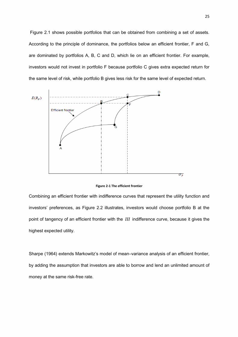
Figure 2.1 shows possible portfolios that can be obtained from combining a set of assets.
According to the principle of dominance, the portfolios below an efficient frontier, F and G,
are dominated by portfolios A, B, C and D, which lie on an efficient frontier. For example,
investors would not invest in portfolio F because portfolio C gives extra expected return for
the same level of risk, while portfolio B gives less risk for the same level of expected return.
Figure 2-1 The efficient frontier
Combining an efficient frontier with indifference curves that represent the utility function and
investors’ preferences, as Figure 2.2 illustrates, investors would choose portfolio B at the
point of tangency of an efficient frontier with the III indifference curve, because it gives the
highest expected utility.
Sharpe (1964) extends Markowitz’s model of mean–variance analysis of an efficient frontier,
by adding the assumption that investors are able to borrow and lend an unlimited amount of
money at the same risk-free rate.
26
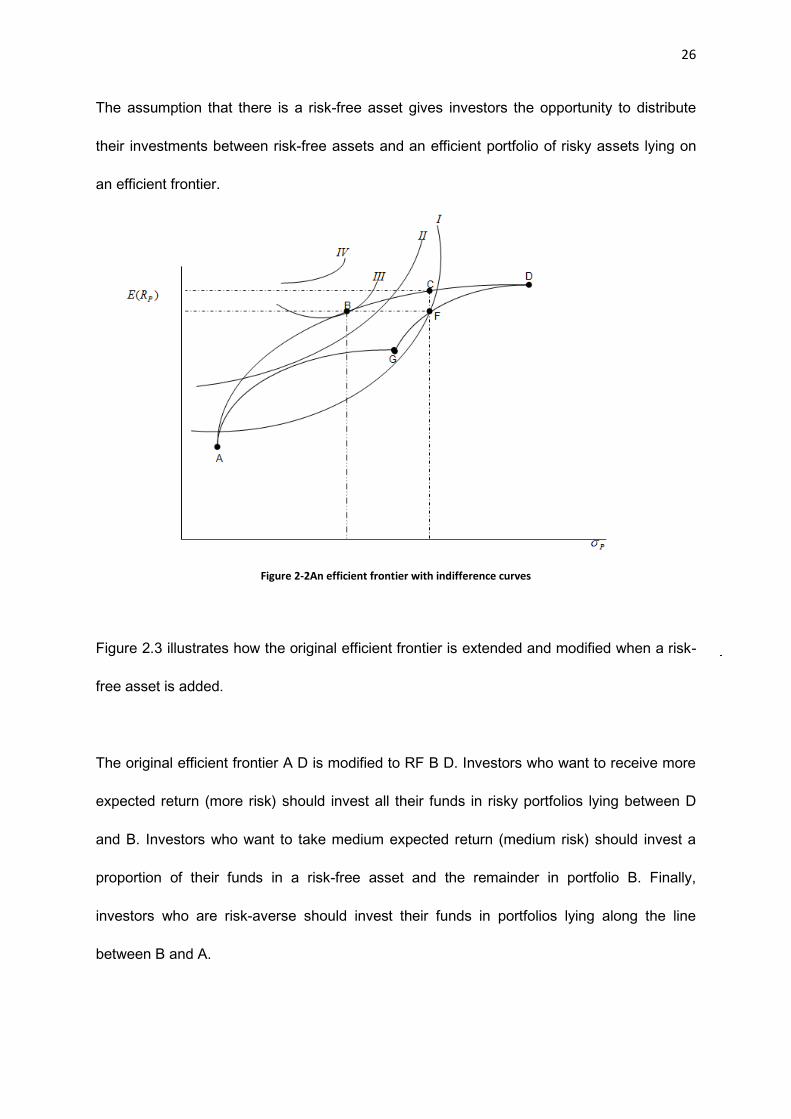
The assumption that there is a risk-free asset gives investors the opportunity to distribute
their investments between risk-free assets and an efficient portfolio of risky assets lying on
an efficient frontier.
Figure 2-2An efficient frontier with indifference curves
Figure 2.3 illustrates how the original efficient frontier is extended and modified when a risk-
free asset is added.
The original efficient frontier A D is modified to RF B D. Investors who want to receive more
expected return (more risk) should invest all their funds in risky portfolios lying between D
and B. Investors who want to take medium expected return (medium risk) should invest a
proportion of their funds in a risk-free asset and the remainder in portfolio B. Finally,
investors who are risk-averse should invest their funds in portfolios lying along the line
between B and A.

27
Figure 2-3 An efficient frontier and risk-free rate
The efficient frontier A D can be modified and extended by assuming investors are able to
borrow an unlimited amount of money and invest this money in risky portfolio B, as Figure
2.4 illustrates.
Figure 2-4 An efficient frontier and opportunity of borrowing

28
By adding the opportunity to borrow, the original efficient frontier A D becomes line A, B, H
and I, where portfolios lying along the line between B and I refer to investors who invest all
their money and borrowed funds in portfolio B.
Combining borrowing and lending opportunities, the interest rate of borrowing the interest
rate of lending or fb RR . The optimal portfolios for each individual investor depend on
investor attitudes to risk, which are represented by indifference curves, as Figure 2.5
illustrates. Investor I is risk-averse, and will invest his funds in a risk-free asset and risky
portfolio U. Investor II is risk-neutral, and will invest all his funds in risky portfolio S. Investor
III is risk-seeking, and will invest all his funds plus borrowed funds in portfolio X.
Figure 2-5 An efficient frontier and opportunity of borrowing and lending

29
Assuming investors are able to borrow and lend at the same risk-free interest rates, the
original efficient frontier becomes a straight line, as Figure 2.6 illustrates. This line is known
as the capital market line and portfolio M is an optimal portfolio that represents the market
portfolio, and all investors wish to hold it.
Since the CML contains efficient portfolios with risk-free assets, the risk for efficient portfolios
lying on the CML is measured by the standard deviation of return14. At the same time, their
expected return is measured by the risk-free rate plus a risk premium that relies upon the
size of the standard deviation of efficient portfolios (Samuels et al, 1995; Lumby and Jones,
2003; Pike and Neale, 2003; McLaney, 2006).
Figure 2-6 Capital market line
14
CML uses the standard deviation to measure risk because all risk is systematic risk according to the principle that the market portfolio is efficient.

30
The equation of CML that represents the risk/return trade-off for efficient portfolios is typically
written as
P
m
fm
fp QQ
RRRP
where:
pP = Expected return on an efficient portfolio.
fR = Risk-free interest rate.
mR = Return on market portfolio.
PQ = Standard deviation of efficient portfolio.
mQ = Standard deviation of market portfolio.
2.2.1.2 Security market line (SML)
The SML, typically known as the CAPM, is derived from the CML to determine the
relationship between the risk and expected return for inefficient portfolios (an individual
investment or share of an individual company). In other words, it describes how individual
risky assets are priced.
In the context of the SML, the risk of inefficient portfolios or individual risky assets is
measured by the beta and the expected return is measured by the sum of three factors: the
risk-free rate of return, risk premium and beta.
The equation of SML or CAPM that represents the relationship between the risk and
expected return for inefficient portfolios or individual risky assets is usually written as
iE fR i mE( )fR

31
where:
iE = Expected return on security or portfolio.
fR = Risk-free interest rate.
i = Beta, which is the amount of systematic risk inherent in the security relative to the
risk of the market portfolio.
mE( )fR = Market risk premium.
The equation of the CAPM shows a linear positive relationship of beta–expected return and
a market equilibrium that, based on this relationship where investors require a higher return
on security, has a higher beta and vice versa. More specifically, in the market equilibrium
where investors adjust securities that hold in their portfolios based on the security price and
its beta, the investors' adjustments result in securities being correctly priced, the market
reaches an equilibrium condition and finally all the assets plot on the SML, as Figure 2.7
illustrates, beta/return trade-off for security (SML).
Figure 2-7 SML

32
2.2.2 Empirical tests of unconditional two-moment CAPM
The aim of this sub-section is to review the previous empirical tests that have examined
unconditional two-moment CAPM, the derivation for which was presented in the previous
sub-section. This model assumed that beta alone explains cross-sectional returns and the
relationship between beta and returns is positive based on two key assumptions: that the
market portfolio is efficient and that asset returns follow a normal distribution. More
specifically, this sub-section focuses on the methodologies and main findings of previous
empirical tests of unconditional two-moment CAPM, which, in general, is opposite to the
predictions of the CAPM and so has encouraged researchers to develop four-moment
CAPM and conditional CAPM. Finally, this sub-section will compare the results of previous
empirical tests of unconditional two-moment CAPM with the empirical results that will be
presented in chapter five.
In order to test the ability of CAPM in explaining cross-sectional return, previous empirical
tests investigated whether:
The relationship between return and beta is positive, in other words, the slope is equal to
the mean market risk premium ( FM RR ).
The relationship between return and beta is linear.
The intercept is equal to the mean risk-free rate.
Other factors do not play any significant role in explaining cross-sectional return.
The following equation of cross-sectional regression was used by previous tests to examine
the implications of the CAPM.

33
it
RtY0 tY1 i tY2
2
i tY3 iS it
where:
it
R = the expected return on security or portfolio.
tY0 = the average coefficient of intercept tY0( ftR )
tY1 = the average coefficient of the slope of risk premium tY1( mtR ftR )
i = the asset or portfolio’s beta
tY2 = the average coefficient of the slope of 2
i
2
i = the measurement of the linear relationship between the expected return and beta
tY3 = the average coefficient of the slope of unsystematic risk
iS = the measurement of unsystematic risk
it = a random error term.
Thus, previous tests assume that:
There is a positive linear relationship between the expected return and beta if tY1 > 0 and
tY2 = 0 . The intercept is equal to the mean risk-free rate if tY0 =0. Others factors do not play
any significant role in explaining cross-sectional return if tY3 = 0 .
Previous empirical tests that examined unconditional two-moment CAPM are reviewed
according to their date and contribution as follows.
Jensen (1969)
The work carried out by Jensen (1969) is one of the earliest empirical tests that examined
the implication of the CAPM. Jensen, by using data of 115 US mutual funds during the

34
period 1945 to 1964, found that the beta only measures the risk of the asset and the
relationship between the beta and return is a positive linear one.
Jacob (1971)
Jacob examined whether the systematic risk of securities is consistent with their average
returns and stabilises the relationship between systematic risk and average returns over
time, by using monthly prices of 1,952 common stocks listed on the New York Stock
Exchange during the period 1925 to 1966. Jacob found that securities with a higher beta
have a lower return and securities with a lower beta have a higher return; his results are the
opposite of the theory of the CAPM.
Black, Jensen and Scholes (1972)
Black et al (1972) developed a version of the CAPM that is known in the literature as Black’s
version or the zero-beta CAPM. This version depends on the relaxation on one of the
assumptions of the CAPM, that there is a risk-free asset and all investors are able to borrow
and lend at a similar common rate of interest; in their version of the CAPM, Black et al used
a portfolio with a zero beta instead of a risk-free asset that all investors are able to borrow
and lend at its rate of interest.
Black’s version can be written as follows:
itR ztR )1( i mR i it
Black et al (1972) pointed out that the value of 0Y zR and 1YmR zR , whereas previous
tests assumed that the value of 0Y fR 0 and 1YmR 0 fR .

35
Black et al (1972) tested a version of the CAPM where the value of 0Y fR and 1YmR
fR and a zero-beta CAPM where the value of 0Y zR and 1YmR zR by using all the
securities listed on the New York Stock Exchange in the period between 1929 and 1966. To
obtain an efficient estimate of the parameters of the CAPM ( 0Y , 1Y ) and reduce the
measurement error in the beta factor, they used time-series and cross-sectional regression.
Black et al (1972) found that the average coefficient of intercept 0Y is significantly different
from zero ( fR ) and the average coefficient of slope 1Y is significantly different from mR(
fR ) when they applied the traditional form of the CAPM. However, they found support for
the zero-beta CAPM where the coefficient of intercept 0Y zR and the coefficient of slope 1Y
mR zR .
More evidence on the examination of the zero-beta CAPM was provided by Fletcher (1997,
2000), who examined the zero-beta CAPM in the UK and international stock markets,
respectively, and found a flat relationship between the beta and the expected return. Also,
Sandoval and Saens (2004), who applied the zero-beta CAPM to Latin American stock
markets, found that the relationship between the beta and return is statistically insignificant.
Javid and Ahmad (2008) examined the zero-beta CAPM in the Karachi stock exchange
based on daily and monthly data of 49 stocks, over the period from 1993 to 2004. Their
study results refer to the risk–return trade-off being positive in some sub-periods, there being
no linear relationship of the beta and return and other factors than beta having an impact on
the return of security.

36
Blume and Friend (1973)
A study by Blume and Friend examined the validity of the CAPM based on US data during
the period from 1950 to 1968. To achieve the purpose of their study, they used a grouping
technique that includes five steps. The first is used to estimate the beta coefficient for each
individual stock by regressing the monthly return on stock on the monthly return on the
portfolio. Second is the formation of portfolios based on the beta for individual stock. Third,
monthly returns are calculated for each formed portfolio. Fourth is to estimate the beta for
each portfolio. Finally, the CAPM is tested by regressing the arithmetic average returns of
the portfolio on their beta coefficients. However, Blume and Friend (1973) summarised that
their empirical study did not confirm the implications of the CAPM.
Fama and McBeth (1973)
Fama and McBeth developed a method to test the validity of the CAPM, this method well
known three steps method and became the standard method to test the CAPM. The first
step is the portfolio formation period, which is used to estimate the beta for individual
securities and form portfolios based on these; grouping individual stocks into portfolios leads
to increasing the accuracy of the estimated beta and reducing the standard error of the
intercept and the slope associated with individual stocks (Lau et al, 1974). The second step
is the portfolio beta estimation period, which is used to estimate the beta for each portfolio
formed in the first step. The third step is the testing period where the SML is tested by using
a cross-sectional regression, to regress the portfolio betas as the independent variable
against the portfolio returns as the dependent variable. Additionally, Fama and McBeth
(1973) asserted that if there is a linear relationship between the betas and the expected
return, the market portfolio must be efficient.

37
Fama and McBeth (1973) applied their method to examine the validity implications of the
CAPM to the NYSE during the period 1926 to 1968; they found powerful support for the
implications of the CAPM.
The empirical studies on the European stock markets by Modigliani et al (1973) and on the
Tokyo stock market by Lau et al (1974) employed a method similar to Fama and MacBeths’
(1973) method and found that the CAPM is applicable to these markets.
Furthermore, Jahankhani (1976), who applied Fama and MacBeth’s (1973) method to test
the prediction of the CAPM during the period from 1947 to 1969, provided evidence that
there is a linear relationship between the beta and the expected return and the beta is a
complete measurement of risk that impacts upon the expected return of a security. On the
other hand, he found coefficients of intercept 0Y and slope 1Y contrary to the prediction of
the CAPM that the risk-free rate of return is less than the intercept and the risk premium is
greater than the slope.
Clare, Priestley and Thomas (1997) compared the performance of Fama and MacBeth’s
method with the non-linear three-stage least squares method. They found that the beta as
an explanatory variable does not explain the cross-section of returns when Fama and
MacBeth’s method is used, while it has explanatory power to explain the cross-section of
returns when the non–linear three-stage least squares method is used.
More recently, Gonzalez (2001) applied Fama and MacBeth’s method to investigate the
implications of the CAPM for the Caracas stock market, and found there is no evidence to

38
support the implications of the CAPM. Michailidis, Tsopoglou, Papanastasiou and Mariola
(2006) used weekly data of the Greek stock market during the period from 1998 to 2002 and
Fama and MacBeth’s method to test the validity of the CAPM. They found that, when the
intercept is different from zero, stock with a higher beta is associated with a lower level of
return and there is linear relationship between the beta and return.
Guermat, Bulkley, Freeman and Harris (2004), who modified the method of Fama and
MacBeth (1973), pointed out that a lack of empirical support for the validity of the CAPM is
due to the employed standard method of Fama and MacBeth (1973), which uses the ex-post
excess market return, which is characterised by volatility and creates high noise of the
estimated slope coefficient. As a consequence, they modified the method of Fama and
MacBeth (1973) by deducting the ex-post market return each month from the estimated
slope coefficient by the method of Fama and MacBeth (1973) to avoid the problem of highly
noisy estimated slope coefficients. Their results provide support for the validity of the CAPM.
Levy (1978)
Levy argued that investors hold portfolios containing a lower number of risky assets than the
market portfolio, which contains all the risky assets available in the market, and also their
portfolios differ in the proportions of risky assets.
As a result, Levy derived a general version of the CAPM (GCAPM), which determines the
expected return on a security by beta and variance. This version of GCAPM can be written
as following:

39
iR 0Y1Y i 2Y
2ˆeiS 3Y
2ˆ
i , where 2ˆ
eiS = the residual variance and 2
ˆi = stands for
the estimate of the i security variance.
Levy (1978) examined the GCAPM on the NYSE during the period 1948–1968 and found
that the variance 2
ˆi explains the price behaviour much better than the beta.
An empirical test by Hawawini et al (1983) examined the GCAPM on the French stock
market over the period 1969–1979 by applying Fama and McBeth’s (1973) method and
found that a linear relationship between the beta and the expected return of security was a
negative; there is no relationship between unsystematic risk, total risk and the stock’s return.
Finally, the value of the intercept is different from zero. Similar results were found by Carroll
and Wei (1988), who examined GCAPM using data of stocks listed on the NYSE over the
period from 1926 to 1985.
Wong and Tan (1991) examined the GCAPM on the Singapore stock market by utilising
weekly data of 72 stocks during the period 1980–1985 and found that the expected return on
security is not related to the beta, residual standard deviation and variance.
Cheung and Wong (1992) tested the GCAPM by using the Hong Kong stock market data
and found that values of 0Y are not different from zero, 1Y 0 , tY2 = 0 and unsystematic
and total risk do not have any role in determining the expected return of security.
Cheung, Wong and Ho (1993) investigated the GCAPM in two emerging Asian stock
markets, Korea and Taiwan, by using data of 166 Korean stocks and data of 70 Taiwanese

40
stocks during the period from 1980 to 1988 and applying Fama and MacBeth’s (1973)
method; their study results revealed that unsystematic risk does not have any impact on the
expected return while total risk does, and they also found that the relationship between the
beta and average return is a positive linear one for the Korean market but a negative non-
linear one for the Taiwanese market.
Reinganum (1981)
Reingaum empirically investigated whether different average returns are related to different
estimated betas. The investigation was performed by using the US data over the period
1964–1979 and utilising a two-step strategy instead of cross-sectional regression, where the
first step is the beta estimation for each individual security and ranking them into one of ten
portfolios according to the estimated beta, and the second step is the return calculation and
using time-series regression to test whether stocks have a high beta associated with a high
return. However, Reingaum found that the returns of high beta portfolios are not significantly
different from the returns of low beta portfolios.
Handa, Kothari and Wasley (1993)
A test carried out by Handa, Kothari and Wasley (1993) investigated the impact of the choice
of the return measurement interval in testing the relationship between the beta and return.
They argued that there are two reasons for the sensitivity of the beta to the return
measurement interval. First, for buy-and-hold returns, the covariance of an asset's return
with the market and variances of the market return do not increase proportionately, implying
that ‘true’ betas are sensitive to the return interval. Second, changes in risk and changes in
the expected rate of return on the market induce a negative serial correlation in returns; if the

41
degree of serial correlation in the return is not the same across subsets of the market
portfolio, relative risk estimates are affected by the return measurement interval.
Based on the above argument, monthly and annual returns were used to measure the return
measurement interval. Using the return of 20 portfolios that were constructed based on their
market values of equity during the period from 1927 to 1988, Handa et al (1993) found that
the CAPM using monthly returns is rejected while the CAPM using annual returns is not and
they suggested that the investment horizon and beta sensitivity to the return measurement
interval are two important factors affecting the risk–return relation.
Fama and French (1992, 1996, 2004)15
The strongest criticism of the CAPM was presented by Fama and French (1992, 1996,
2004). They investigated the basic prediction of the CAPM by employing almost 50 years
(1941–1990) of the US securities’ return data and they extended the period of analysis from
1928 to 2003 in their study (2004). They found that the intercept of cross-section regression
is greater than the average risk-free rate and the coefficient on the beta is less than the
average excess market return. Moreover, Fama and French (1992, 1996, 2004) in their
studies concluded that the CAPM is poor–poor enough and rejected the whole theory of the
CAPM. Fama and French (1992) proposed a three-factor model that includes the beta, size
and book-to-market value and they found that the three-factor model outperforms the CAPM
to explain the cross-sectional returns.
15
The reason for presenting the studies of Fama and French in which the developed model includes the impact of other variables (size and book-to-market value) here, and not with studies that investigated the influence of firm-specific factors, is that these studies are considered by many empirical studies to be evidence against the validity of CAPM. In addition, their model (the three-factor model) is an alternative to CAPM.

42
Faff (2001) examined the three-factor model of Fama and French on the Australian stock
market and found strong support for both variables of size and book-to-market value. For
more empirical evidence on testing the three-factor model, Drew, Naughton and
Veeraraghavan (2003) compared the performance of the CAPM with the three-factor model
on the Asian emerging markets; they found that the three-factor model provided a better
indication of the asset risk and estimates of the required rate of return than the CAPM. Guidi
and Davies (2000) confirmed Fama and French's (1992) evidence that the beta, size and
book-to-market value play an important role in explaining cross-section returns on the UK
stock market.
The three-factor model was tested further by Daniel, Titman and Wei (2001) on the
Japanese stock market. Their tests indicate that the three-factor model does not have the
explanatory power to explain cross-section returns. Eom and Park (2008) applied the three-
factor model to the Korean stock market. Their study findings indicate the rejection of the
three-factor model.
Amihud, Christensen and Mendelson (1992) argued that Fama and French’s study and
other empirical studies covered their study as a previous study reporting that the beta is
dead was greatly exaggerated. Amihud et al (1992) pointed out that Fama and French's
study providing evidence against the validity of the CAPM is due to the estimation
methodology of Fama and MacBeth (1973) and an ordinary least squares (OLS), which is
used to estimate the parameters of the CAPM ( 0Y , 1Y ).

43
Statistically, Amihud et al (1992)16 suggested that if residuals for each period are cross-
sectionally uncorrelated and homoscedastic across assets and over time, the employment of
OLS in the joint pooled estimation (panel data) would be optimal. Since the residuals for
each period are cross-sectionally correlated and heteroscedastic across portfolios, and the
variances change over time, while coefficients of the CAPM equation estimated by the OLS
are unbiased and consistent, the generalised least squares (GLS) would be the optimal
method to test the pooled joint time series and cross section.
Amihud et al (1992) examined the joint pooled cross-section and time-series use of the GLS
and Fama and MacBeth’s (1973) method’s use of both OLS and GLS by utilising data of
stocks traded on the New York Stock Exchange during the period from 1953 to 1990.
Their results indicated that there was a significant positive return–beta relationship when
they utilised joint pooled cross-section and time-series use of the GLS and an insignificant
return–beta relationship when they employed Fama and MacBeth’s (1973) method’s use of
OLS. However, they found a significant positive return–beta relationship when they used
Fama and MacBeth's (1973) method’s use of GLS. Amihud et al (1992) concluded that the
beta is still an essential factor in asset pricing.
Jagannathan and Wang (1993) and Jagannathan and McGrattan (1995) argued that Fama
and French’s (1992) finding of a statistically insignificant relationship between the beta and
return is not economically an important reason to reject the CAPM.
16
The study by Amihud et al (1992) is the first study presented in this sub-section that uses panel data or pooled joint time series and cross sections to test the CAPM. The panel data method will be key method in this study to test asset pricing model.

44
Jagannathan and Wang (1993, 1996) demonstrated that Fama and French’s study and other
empirical studies found a statistically insignificant relationship between the beta and return
because unreasonable assumptions are used in the empirical testing of the CAPM. These
assumptions are: the stock market index is a market portfolio that contains all the assets in
the economy and the beta of the asset remains constant over time.
Kothari, Shanken and Sloan (1995) tested the CAPM and three-factor model from 1927–
1990 by using annual data instead of monthly data and an equally weighted index and
value-weighted index as a proxy for the market portfolio.
The results of their study indicated that there exists a significant relationship between the
beta and expected return when the annual data are used and the annual compensation for
systematic risk ranges from about 8.9% to 11.7% when the equally weighted index is used
and 6.2% to 8.9% when the value-weighted index is used. In addition, Kothari et al (1995)
found a weak relationship between the expected return and book-to-market value when
annual data are used.
Pettengill et al (2002) tested the three-factor model in all markets and in up and down
markets and found that the book-to-market value and size did not explain the cross-sectional
returns in two cases, whereas Howton and Peterson (1998) found that the book-to-market
value is an important variable in a down market only and size is an important variable only in
January and in a down market. Furthermore, Perold (2004) summarised that:
“... The size and book to market cannot be risk factors also Fama-French factors are
identified, the forecast power of their model will be in doubt and the applications will
be limited”.

45
Shanken and Zhou (2007)
Shanken and Zhou compared the performance of the multivariate approach, ordinary least
squares (OLS), weighted least squares (WLS), generalised least squares (GLS), maximum
likelihood (ML) and generalised method of moments (GMM) to test the CAPM and three-
factor model. They used the two-pass procedures of Fama and MacBeth to estimate OLS,
WLS and GLS and they also used the following equations to estimate the performance of
OLS, WLS, GLS, ML and GMM to test the CAPM and three-factor model:
itR i
1i tf1 it
tRE[ 0] Y 11 YN 1
itRftr i 1i tmf ,( ftr 2) i tSMBf , 3i tHMLf , it
itRE(ftr ) 0Y
1Y 1i 2Y 2i 3Y3i
where:
itR = the return on asset i in period t .
tf1 = the realization of the market factor in period t .
T = the time-series length.
N = the number of assets.
SMBf = the book-to-market value.
HMLf = the size.
Using data from January 1964 to December 2003, Shanken and Zhou (2007) found that ML
is more precise for estimating the CAPM and the three-factor model than OLS, WLS, GLS
and GMM, ML and GLS are more efficient than OLS and WLS for estimating the CAPM and
OLS and WLS are less biased than GLS.

46
Girard and Omran (2007)
They investigated the validity of unconditional CAPM in five Arab stock markets – Egypt,
Jordan, Morocco, Saudi Arabia and Tunisia – during the period from 1997 to 2001. 130
stocks from five markets were included in the sample. The method they used to investigate
the validity of unconditional CAPM was to compare the yearly actual returns on stocks with
their returns based on the CAPM. By applying this method Girard and Omran found that a
constant beta is not a good proxy for risk in Arab stock markets, which are considered to be
thinly traded emerging markets.
Bruner, Li, Kritzman, Myrgren and Page (2008)
They tested market integration in developed and emerging markets by using the global and
domestic CAPM, and data of 48 countries during the period from January 1994 to July 2004.
Their results showed that emerging markets are less integrated than developed markets and
the domestic CAPM tend to yield significantly better results than the global CAPM in
emerging markets, due to market segmentation.
Cheng, Parvar and Rothman (2010)
They also tested the CAPM in nine Middle East and North African (MENA) markets (Bahrain,
Egypt, Jordan, Morocco, Oman, Kuwait, Israel, Turkey and Saudi Arabia). Their objectives
were to investigate the validity of CAPM and to check whether these markets are integrated
with or segmented from global equity markets. To test international CAPM and hence stock
market integration, they considered the excess returns for each the national market as
excess returns of portfolio and excess returns of an index composite of international
markets, the DJG as excess returns of market portfolio. By using international CAPM Cheng

47
et al (2010) found that Israel and Turkey are integrated with global equity markets, in most
other MENA markets the domestic CAPM outperforms global CAPM.
Grauer and Janmaat (2010)
Grauer and Janmaat pointed out that the results of testing the CAPM are sensitive to how
individual stocks are grouped into portfolios, and also are sensitive to which zero-weight
portfolios are employed in the tests. Therefore, they proposed repackaging the data with
zero-weight portfolios procedure as an alternative to the grouping procedure that was used
to reduce measurement error to test the CAPM.
According to their procedure the portfolios are sorted by beta; the returns on the lowest beta
portfolio is replaced with the returns on the lowest beta portfolio minus the returns on the
highest beta portfolio; the returns on the second lowest beta portfolio are replaced with the
returns on the second lowest beta portfolio minus the returns on the second highest beta
portfolio, etc. until half the portfolios are replaced. By repackaging the data with zero-weight
portfolios procedure, OLS and GLS Grauer and Janmaat found powerful support for the
CAPM.
From the above review of the previous empirical tests of unconditional two-moment CAPM, it
can be concluded that some early tests of unconditional two-moment CAPM, such as the
tests of Jensen (1969), Black et al (1972) and Fama and McBeth (1973), provided evidence
confirming the implications of CAPM. More recent tests of the CAPM, like those conducted
by Reingaum (1981), Fama and French (1992, 1996, and 2004), Drew and Veeraraghauan
(2003) and Girard and Omran (2007), provided results that contradict the implications of the

48
CAPM. The results of recently tests of the CAPM have led many empirical studies to
extended unconditional two-moment CAPM by adding variables related to firm-specific
factors instead of using variance as a measure of total risk and standard deviation of
residual as measure of unsystematic risk to represent risk associated with firm-specific
factors. This extension by adding firm-specific factors is discussed in the next sub-section on
the impact of other variables.
2.2.2.1 The impact of other variables
The purpose of this sub-section is to show the importance of firm-specific factors in
explaining the cross-section of returns, in addition to beta. Empirical studies by Hawawini et
al (1983), Wong and Tan (1991), Cheung and Wong (1992) and Cheung et al (1993) found
that variance, which represents the part of risks related to firm, and standard deviation of the
residual, which represent all risk related to a firm, were insufficient at explaining the cross-
section of returns. In order to represent firm-specific factors, other empirical tests used
fundamental variables17 such as size, leverage, ratio of cash flow to stock price, past sales
growth, P/E ratio and book-to-market value (Claessens, Dasgupta and Glen, 1995;
Akdeniz, Altay-Salih and Aydogan, 2000; Tang and Shum, 2006) instead of statistical
variables. This approach is known in the financial literature as anomalies 18 or
misspecification of the CAPM. These anomalies are presented as follows:
17
Some empirical studies such as studies of Chan, Hamao and Lakonishok (1991) Fundamentals and stock returns in Japan, He and Ng (1994) Economic forces, fundamental variables, and equity returns and Lam and Spyrou (2003) Fundamental variables and the cross-section of expected stock returns: the case of Hong Kong refer to firm-specific factors as fundamental variables. 18
Other empirical studies, such as those of Fama and French (1996) Multifactor explanations of asset pricing anomalies, Ho, Strange and Piesse (2000) CAPM anomalies and the pricing of equity: evidence from Honk Kong market and Avramov and Chordia (2006) Asset pricing models and financial market anomalies, refer to firm-specific factors as anomalies. Fama and French (1996) find that anomaly patterns in average stock returns are not explained by the CAPM but can be explained by firm-specific factors.

49
The impact of the firm's size
Banz (1981) empirically examined the relationship between the firm's size, which is
measured by the total market value of the NYSE commons stocks and returns, and found
that small firms have a higher risk than large firms and the impact of the firm's size is not
linear. Moreover, Banz (1980) concluded that CAPM is misspecified.
Despite this evidence to support the relationship between return and size, subsequent
empirical tests that re-examined the findings of Banz's study provided mixed results about
the ability of the size factor to explain the cross-section of return.
The results of Fama and French’s study (1992) revealed that the cross-section of return is
associated with size. Contrary to the findings of Banz (1980) and Fama and French (1992),
Lakonishok and Shapiro (1984) found that size is only an important variable for the total
period, not for sub-periods, whereas other empirical tests, performed by Tinic and West
(1986), Chan and Chen (1988), Berk (1996) and Manjunatha, Mallikarjunappa and Begum
(2007), showed that the expected return of stocks is unassociated with size.
Leverage
Bhandari (1988) documented that leverage, which is measured by the debt-to-equity ratio, is
an important variable to explain the cross-section of return and a natural measurement of a
firm's risk where an increase in leverage leads to an increased risk of the firm. Using the US
data during the period from 1948 to 1981, Bhandari (1988) found a positive relationship
between the expected return and leverage. However, Fama and French (1992), who used

50
two variables, book assets/market equity ratio and book assets/book equity, to measure the
role of leverage to explain the cross-section of return, found that there was a relationship
between the expected return and the two measurements of leverage, but the relation
between the book assets/market equity ratio and the expected return was always positive
whereas the relation between the book assets/book equity ratio and the expected return is
always negative. Fama and French (1992) argued that the book-to-market value ratio can
explain the effect of leverage on the expected return.
Earnings yields, cash flow and liquidity
In addition to size and leverage, Jaffe, Keim and Westerfleld (1989), Chan et al (1991),
Davis (1994), Claessens et al (1995) and Strong and Xu (1997) found that earnings yields
and cash flow have explanatory power to explain the cross-section of returns. Holmstrom
and Tirole (2001), Acharya and Pedersen (2005) and Bali and Cakici (2008) found that
liquidity plays an important role in determining the expected return of stocks.
However, the results of empirical tests support the view that cross-sectional differences in
average returns are not only determined by the market risk, as prescribed by the CAPM, but
also by firm-specific factors (Avramov and Chordia, 2006). However, data on firm-specific
variables for Arab stock markets are unavailable, as mentioned in chapter one. In addition,
this study focuses on systematic risk factors related to the market risk variables beta, co-
skewness and co-kurtosis, which will be discussed in the next section, and factors related to
macroeconomic variables and market liquidity, which will be discussed in chapter three.
Campbell (1996) and Fletcher and Kihanda (2005) claimed that factor models that include
anomalies as explanatory variables of stocks’ behaviour suffer from the problem that the

51
factors are not motivated by theory. Daniel and Titman (1997) pointed out that firm-specific
factors are firms’ characteristics rather than risk factors, and these characteristics are a
determinant of expected return This study will use standard deviation of residual as the
measure of unsystematic risk to represent firm-specific variables.
Subsequent sections attribute weak support as an implication that unconditional two-moment
CAPM to inexistent a truly diversified market portfolio (one of the parameters used to
estimate beta and for testing CAPM). Roll and Ross (1994) argued that a positive, exact
cross-sectional relationship between ex-ante expected return and beta holds and that no
variable other than beta can explain any part of cross-section returns if the market portfolio is
efficient. Pettengill et al (1995) pointed out that absence of a positive relationship between
beta and return due to the return of market portfolio is less than risk-free return. The theory
of APT does not require a particular portfolio to be mean variance efficient.
To show the common perspective between the impact of others variables which discussed in
this sub-section, conditional CAPM which will be discussed in section 2.4 and the theory of
APT which will be discussed in chapter three is the market portfolio and whether it is mean-
variance efficient and its return is more than risk-free return. The problems with the market
portfolio that are associated with the testing of CAPM are known in the financial literature as
Roll’s critique, and this will be discussed in the following sub-section.
2.2.2.2 Roll’s critique
In his critique of the asset pricing theory’s tests, Roll (1977) argued that CAPM is testable in
principle, but is untestable when applied to empirical work, because the market portfolio is

52
not observable and mathematical equivalence between the mean-variance efficiency of a
reference portfolio and linearity relationship between return and beta of asset.
Roll (1977) pointed out that the traditional CAPM is testable if the exact composition of the
true market portfolio is known and used in empirical investigations. The phrase ‘composition
of the true market portfolio’ implies that portfolio includes all types of assets. Furthermore, he
pointed out that true market portfolio is mean-variance efficient. Roll (1977) exposed the fact
that if a true mean-variance efficient market portfolio is exist, this would support the
assumptions of CAPM; that there is a positive relationship between beta and return, beta is
the only measure of risk, the relationship between beta and return is linear and market return
must exceed risk-free return.
Roll (1977) criticised empirical studies that used stock market indices as proxies for market
portfolios. He stated that a market index is subject to two difficulties. First, the chosen proxy
itself might be mean-variance efficient, but this does not establish that the true market
portfolio is also on the mean-variance efficient frontier. Secondly, the chosen proxy may
become inefficient; however, this means nothing regarding the true market portfolio’s
efficiency. Additionally, Roll (1977) pointed out that the exact composition of the true market
portfolio becomes unimportant when reasonable proxies are highly correlated with each
other and with the true market portfolio, whether or not they are mean-variance efficient.
With respect to a linear relationship between ex-post mean-variance efficient portfolio and
individual assets Roll (1977, p. 130) stated that
“….. in any sample of observations on individual returns, regardless of the generating
process, there will always be an infinite number of ex-post mean-variance efficient

53
portfolios. For each one, the sample `betas’ calculated between it and individual
assets will be exactly linearly related to the individual sample mean returns. In other
words, if the betas are calculated against such a portfolio, they will satisfy the linearity
relation exactly whether or not the true market portfolio is mean-variance efficient.”
By reviewing the earliest empirical tests of unconditional two-moment CAPM carried out by
Black et al (1972), Blume and Friend (1973) and Fama and MacBeth (1973), as presented in
sub-section 2.2.2, Roll (1977) found evidence that a mean-variance efficient market portfolio
was supported only by the study of Black et al (1972).
However, all the above discussion of Roll’s critique was regarded the existence of the a
mean-variance efficient market portfolio. As a further argument about the mean-variance
efficiency of market portfolio, Roll (1977) addressed the issue of how to test the mean-
variance efficiency of a known composition portfolio. Related to this issue Roll (1977, p.
131) added
“…. A direct test of the proxy’s mean-variance efficiency is difficult computationally
because the full sample covariance matrix of individual returns must be inverted and
statistically because the sampling distribution of efficient set is generally unknown. ….
Testing for the proxy’s efficiency by using the return/beta linearity relation also poses
empirical difficulties; the two-parameter theory does not make a prediction about
parameter values but only about the form (linear) of the cross-sectional relation.
Thus, econometric procedures designed to obtain accurate parameter estimates are
not very useful. Specifically, the widely-used portfolio grouping procedure can support
the theory even when it is false. This is because individual asset deviations from
exact linearity can cancel out in the formation of portfolios."
Dimson and Mussavian (1999) in their study entitled “Three centuries of asset pricing”
summarised Roll’s critique in four main points; first the definition of market or market
portfolio in the CAPM theory of CAPM is not a single equity market index, but an index
containing all kinds of asset. The market index must therefore include bonds, property,
foreign assets, human capital and anything else, tangible or intangible, that adds to the

54
wealth of mankind. Secondly, market portfolio must be determined in order to test CAPM.
Thirdly, tests of the CAPM are tests of the mean-variance efficiency of the portfolio that is
taken as the market proxy; therefore, findings that are evidence against the efficiency of a
given portfolio say nothing about whether or not the CAPM is correct. Finally, the methods
Black et al (1972) and Fama and MacBeth (1973) used to test the CAPM suffer from the
errors-in-variable problem, because independent variables in the second step (betas) are
estimates from the first step regression, which typically causes the estimated risk premium to
be smaller in magnitude than the true risk premium.
Dimson and Mussavian (1999) stated that in time researchers will deal with the Roll critique
to allow testing of the CAPM. Ross (1976) developed the APT as an alternative model to
CAPM, in order to overcome the problems of market portfolio associated with the testing of
the CAPM, as APT does not require a particular portfolio to be mean variance efficient as
CAPM does.
According to Roll’s critique about the existence of the true market portfolio and how to test
the mean-variance efficiency of a market portfolio, Shanken (1987) investigated CAPM by
using multivariate proxies: a stock index proxy (equal-weighted stock index) and market
index including stocks and bonds. He found that CAPM is invalid and that the results are the
same using a stock index alone, or together with a bond index.
To overcome the challenges outlined in the above discussion of Roll’s critique, which relate
to the existence of a true market portfolio and its efficiency, some empirical studies have
tested the impact of other variables related to firms, as presented in sub-section 2.2.2.1.

55
Conditional CAPM, which will be presented in section 2.4, and the theory of APT, which will
discussed in chapter three, also attempt to deal with the fundamental problem of CAPM
which is the market portfolio. The next section deals with another fundamental problem of
CAPM, which occurs when asset returns are not normal distributed and there exist third and
fourth moments (skewness and kurtosis).

56
2.3 Theory of unconditional four-moment CAPM
Recently, empirical tests of the unconditional two-moment CAPM that was reviewed in the
previous sub-section showed results opposite to those predicted by the CAPM. As
mentioned in chapter one, some studies attribute the reason for the failure of recent tests of
two-moment CAPM to capture the cross-sectional variation in average stock returns to one
of the assumptions of the CAPM, which is that asset returns follow a normal distribution and
that higher moments in the return distribution beyond mean and variance (skewness and
kurtosis) do not have any influence on stock returns and investors’ preferences, and thus
investors’ decisions. However, when stock returns are observed empirically, they do not
follow a normal distribution and skewness and kurtosis do have an influence on stock return,
particularly for Arab stock markets. Chapter five will show the results of the normality tests
for these markets.
To support the extension of the CAPM to incorporate the influence of co-skewness and co-
kurtosis and their importance to explain variation in stock returns, this section will be divided
into two sub-sections: the first shows the derivation of four-moment CAPM and the second
empirically tests four-moment CAPM.
2.3.1 Derivation of unconditional four-moment CAPM
According to the CAPM, asset returns are normally distributed, and the first two-moment
mean and co-variance are sufficient for determining the pricing relationship, and also three-
and four-moment or higher (co-skewness and co-kurtosis) would be expected to have mean
values of zero, since no normality is usually characterised by the asymmetric and leptokurtic

57
or existence of skewness and kurtosis. In addition, stock return distribution empirically is
observed to be asymmetric and leptokurtic, which implies stock return does not follow
normal distribution, and hence investors prefer stock with high-positive co-skewness and low
co-kurtosis. Researchers suggest that CAPM must incorporate co-skewness and co-kurtosis
in order to describe asset return distributions.
Kraus and Litzenberg (1976) extend the CAPM to incorporate co-skewness. Skewness
measures the degree of asymmetry of a return distribution (Chiao et al 2003 pp. 359).
Positive (negative) skewness refers to a distribution with an asymmetric tail extending
toward more positive (negative) values Liow and Chan (2005). Lin and Wang (2003)
suggested three possible explanations for the presence of asymmetry in stock returns and
hence incorporate co-skewness in the CAPM: the presence of agency problems and limited
liability, the correlation between price and volatilities as well as compound return in a multi-
periodic framework.
According to three-moment theory, investors prefer the right skewness because it indicates
to the greater probability of obtaining a return above the mean than below the mean and
they will pay for this preference by requiring lower return Vines et al (1994). Also, The theory
of three-moment CAPM assumes that investors prefer positive return skewness in their
portfolio, and positive or negative co-skewness in individual assets relying on the skewness
in the market portfolio. In other words, the three-moment CAPM states that in periods when
market return has right skewness distribution, assets with a positive co-skewness would also
likely exhibit right skewness, which decreases required return. On the other hand, assets
with a negative co-skewness would likely show left skewness distribution, which increases

58
required return. Therefore, in periods when market return has right skewness distribution,
the sign of asset skewness should be negative. When market return is skewed to the left,
investors who have assets with positive co-skewness require a higher return, while investors
who have asset with negative co-skewness would be willing to accept a lower return.
Consequently, in periods, when market return has left skewness distribution, the sign of
asset skewness should be positive.
Furthermore, Fang and Lai (1997) extend the CAPM to incorporate effect of co-kurtosis in
addition to co-variance and co-skewness, this extension is well known as four-moment
CAPM. Fang and Lai (1997) stated that kurtosis refers to the extent to which the distribution
tends to have relatively large frequencies around the centre and in the tails of the
distribution. Kurtosis higher (lower) than three indicates a distribution more peaked (flatter)
than a normal distribution (Liow and Chan, 2005).
Yang and Chen (2009) emphasised that not taking co-kurtosis into account may lead to bias
in the estimates in tests for the risk-return trade-off. Hwang and Satchell (1999) pointed out
that there are two possible explanations for the presence of co-skewness and co-kurtosis in
asset returns in emerging markets: non-stationary, resulting from growing degrees of market
integration; and the influences of non-economic factors, such as political and social factors.
Bekaert et al (1998) in their study on distributional characteristics of emerging market returns
and asset allocation, proved extensive analysis regarding existence of skewness and
kurtosis in emerging markets, changing skewness and kurtosis over time and the

59
relationship between skewness and kurtosis and a number of fundamental characteristics of
emerging countries.
In terms of existence of skewness and kurtosis in emerging markets, Bekaert et al (1998)
found that 17 of 20 countries had positive skewness in returns, and 19 of 20 countries had
excess kurtosis. As a consequence, they argued that the standard mean-variance analysis
or two-moment CAPM is somewhat problematic with respect to emerging markets. With
respect to time-varying characteristics or change skewness and kurtosis through time,
Bekaert et al (1998) split the sample between the 1980s and 1990s because many of the
capital market liberalisation occurred in the early 1990s. They found that more countries had
positive skewness in the 1990s than in the 1980s, and the degree of kurtosis for many
countries was reduced in the 1990s compared to the 1980s, and they explained that
phenomenon was caused by the integration process in many emerging markets. In terms of
the relationship between skewness and kurtosis and a number of fundamental
characteristics of emerging countries, they found that skewness is negatively related to
country risk ratings and GDP growth, while it is strongly positively related to inflation, book-
to-price and the beta versus the MSCI world index. Kurtosis is found to be negatively related
to country risk ratings, market capitalisation and GDP growth, and it is positively related to
inflation, book-to-price and beta.
In order to derive four-moment CAPM, investor’s wealth in the end of period is written as
follows:
i
ffii RRW
i
pipiW

60
i
pipiW SS
i
pipiW KK
where
iR expected return on risk asset 1i
fR risk-free rate 1
i investor’s holding proportion in the risky asset i
f investor’s holding proportion in the risk-free asset
ip measure of co-variance which is calculated as follows 2/12)
~(
)~
)(~
(
PP
Ppii
RRE
RRRRE
ipS measure of co-skewness which is calculated as follows 3/13
2
)~
(
)~
)(~
(
PP
Ppii
RRE
RRRRE
ipK measure of co-kurtosis which is calculated as follows 4/13
3
)~
(
)~
)(~
(
PP
Ppii
RRE
RRRRE
The four-moment CAPM can be written as follows
im
W
im
W
im
W
fi kdk
wdS
ds
wd
d
wdRR
where
wd the expected terminal wealth
ww s, and wk the second , third and fourth moments of the terminal wealth respectively.
i 2)(
)])([(
mtmt
mtmtii
RR
RRRR
iS 3
2
)(
)])([(
mtmt
mtmtii
RR
RRRR
iK4
3
)(
)])([(
mtmt
mtmtii
RR
RRRR

61
From above equations four-moment CAPM can be rewritten as follows
)()()( fmifmifmipfi RRKRRSRRaRR
According to four-moment CAPM, investors require more return for increasing co-variance
and co-kurtosis and less return for increasing co-skewness. In other words, the relationship
between return and co-variance and co-kurtosis is positive. While the relationship between
return and co-skewness is opposite to market skewness, where in period market return is
skewed to the right the relationship between return and co-skewness will be negative, in
period market return is skewed to left the relationship between return and co-skewness will
be positive.
2.3.2 Empirical tests of unconditional four-moment CAPM
Previously, sub-section 2.2.2 focused on the importance of the mean and variance to
investors who prefer to be closer to the mean and are averse to variance. It also showed the
power of these measures to explain cross-sections. However, most previous empirical tests,
as also presented in sub-section 2.2.2, provide results inconsistent with the prediction of the
CAPM. As a result, sub-section 2.3.1 showed that the prior empirical tests of unconditional-
two moment CAPM were unsuccessful at capturing the cross-sectional variation in average
stock returns because they do not take into account effect of co-skewness and co-kurtosis. It
also showed how unconditional two-moment CAPM has been modified to include the effects
of co-skewness and co-kurtosis to explain the cross-section of stock returns. To present how
unconditional four-moment CAPM provides better results empirically than unconditional two-
moment CAPM, empirical tests of four-moment CAPM will be discussed in the following sub-

62
sections: the first sub-section presents empirical tests of unconditional three-moment CAPM,
while the second sub-section presents empirical tests of unconditional four-moment CAPM.
2.3.2.1 Empirical tests of unconditional three-moment CAPM
Kraus and Litzenberg (1976) pointed out that previous empirical tests did not find any
support for two parameters the CAPM attributes to the omission effect of the third moment
(systematic skewness) on the expected return, which is ‘the relationship between the asset’s
excess return with the square of the unexpected systematic (market) return’ (Liow and Chan,
2005). Moreover, Post, Vliet and Levy (2008) pointed out that co-skewness is a supplement
to the beta, which can explain a substantial part of the cross-sectional variation of the mean
return not explained by the beta.
Kraus and Litzenberg (1976), who developed the first version of the CAPM to incorporate co-
skewness, assumed that investors are averse to standard deviation and prefer positive
skewness.
Empirically, the following equation is used to test the effects of skewness:
0YR 1Y i 2Y i i
where: 2Y = the coefficient of skewness and i = skewness. The three-moment CAPM
assumes that 00 Y , 01 Y and 2Y has the opposite sign of3
Mm .
The empirical studies that have tested the impact of co-variance and co- skewness are:

63
Kraus and Litzenberg (1976)
Kraus and Litzenberg tested the three-moment CAPM on the NYSE over 30 years from 1926
to 1970 by utilising a procedure similar to that of Black et al (1972) and Fama and MacBeth’s
(1973) procedure, where the first step, from January 1926 to December 1935, was the
portfolios’ formation by estimating the beta and skewness for each security and the
securities were ranked into portfolios based on their estimated beta and gamma. The second
step, from January 1936 to December 1937, was used to calculate the beta and gamma19 for
each portfolio formatted in the previous step and this procedure was repeated for the period
from 1960 to 1969. The third period was the test period.
Kraus and Litzenberg employed the OLS to estimate 0Y , 1Y and 2Y ; their study results are in
line with the prediction of the three-moment CAPM where the value of 0Y = 0, 1Y > 0, 2Y has
the opposite sign of 3
Mm and systematic skewness, not total skewness, determines a
security price.
Vines et al (1994) employed the third-moment CAPM model of Kraus and Litzenberg in REIT
returns and found that systematic skewness is not priced. In a related work, Omran (2007)
applied the three-moment CAPM to the Egyptian stock market by utilising weekly data of 41
companies during the period 2001 to 2002. The methodology used to test the validity of the
CAPM was a two-step regression. The first step is a time-series regression to systematic
and unsystematic risk; the second step is a cross-sectional regression where the average
returns for the individual stock are regressed against its beta,2 unsystematic risk and
19
Some studies use term gamma to refer to skewness.

64
skewness. The results showed that systematic risk and skewness are important variables to
determinate the expected return.
Friend and Westerfield (1980)
Friend and Westerfield carried out a comprehensive test of the three-moment CAPM
developed by Kraus and Litzenberger (1976) by using two types of market portfolio: one
included bonds and stocks and the other included stocks only. They constructed the first
type of portfolio by combining Standard and Poor’s 500 index, which includes all common
stocks from 1947 to 1964, the NYSE index from 1947 to 1976, the Salomon Brothers’s
index, which includes all corporate bonds from 1969 to 1976, Moody’s bond index from 1947
to 1973, the US Government bond index from 1947 to 1973 and Salomon Brother’s
government bond yields from 1974 to 1976. They also constructed the second type of
portfolio by combining Standard and Poor’s 500 index from 1947 to 1964 and the NYSE
index from 1947 to 1976, which includes all common stocks only. Moreover, their
comprehensive test of the three-moment CAPM used two measures of the market portfolio:
a value-weighted index and equal-weighted index and an individual asset and portfolio of
assets to test the validity of the three-moment CAPM.
Friend and Westerfield (1980) found some evidence that systematic skewness is priced,
which supports Kraus and Litzenberger’s three-moment CAPM; a different index used for the
market portfolio leads to a different ability of systematic skewness to explain the asset price,
and the value of the intercept is significantly different from zero.

65
Lim (1989)
Lim argued that previous studies that had tested Kraus and Litzenberger’s three-moment
CAPM depended on cross-sectional regressions and were affected by measurement error
and yielded inefficient estimations for the parameters of the model. To avoid this problem,
they suggested using generalised method of moments (GMM).
Lim (1989) tested Kraus and Litzenberger’s three-moment CAPM on the NYSE during the
period 1933 to 1982 by applying GMM, and found some evidence that systematic skewness
can explain a substantial part of the cross-section. However, Torres and Sentana (1998)
examined the three-moment CAPM in the Spanish stock market during the period January
1963 to December 1992 by using a method similar to that used by Lim (1989), and found
that skewness is not an important factor to explain the cross-sectional variation of expected
returns.
Lawrence, Geppert and Prakash (2007)
They tested and compared the performance of unconditional two- and three-moment CAPM
and three-factor model. They used Fama and French 25 portfolios data starters from July
1963 to December 2002 and the time-series and the cross-sectional tests to examine and
compare three asset pricing models.
For two-moment CAPM the results of time-series regression showed that beta is found to be
significant for all 25 portfolios but constant of 12 portfolios is found to be significant which is
inconsistent with the theory of CAPM. Also, the results of time-series regression showed that
the average R2 value for the 25 portfolios is 0.72. Contrarily, the results of cross-sectional

66
regression showed that beta is found to be insignificant, while constant is significant and R2
is 0.26. These results provided evidence against exceptions of the CAPM.
With respect to three-moment CAPM the results of time-series regression showed that
constant is significant for 14 portfolios and beta is significant for all 25 portfolios whereas co-
skewness is insignificant for 11 out of 25 portfolios. The average R2 value for the 25
portfolios remains approximately the same as with two-moment CAPM (0.72). Opposite to
predictions of three-moment CAPM the results of cross-sectional regression showed that
constant is significant while beta and co-skewness is insignificant and the average R2 is
0.40.
For the three-factor model the results of time-series regression showed that beta, size and
book-to-market are significant for all 25 portfolios whereas constant is insignificant. The
results of cross-sectional regression indicated that beta, book-to-market value and constant
are significant, while size is insignificant. From the results of the time-series and the cross-
sectional tests Lawrence et al (2007) concluded that the three-factor model outperforms the
two- and three-moment CAPM.
The mixed results about the ability of co-skewness to explain the cross-sectional variation of
expected returns that were provided by the previously discussed empirical studies of
unconditional three-moment CAPM have encouraged other empirical studies to investigate
the ability of four-moment CAPM to determines a security’s price; this will be discussed in
the next sub-section.

67
2.3.2.2 Empirical tests of unconditional four-moment CAPM
Fang and Lai (1997) argued that the expected return is not explained by systematic variance
and systematic skewness only, but also by systematic kurtosis. They assumed that
increasing the systematic variance and systematic kurtosis led to increasing the expected
return, and decreasing the systematic skewness led to increasing the expected return. In
other words, investors demand more expected return as compensation for bearing the
systematic variance and the systematic kurtosis and also investors will have to forgo the
expected return if they take the benefit of increasing the systematic skewness.
The following equation is used by empirical studies to test four-moment CAPM
iR fR 1Y i 2Y S 3Y iK
The unconditional four-moment CAPM holds if 1Y and 3Y 0 and 2Y has a sign opposite to
the skewness of the market portfolio. Among empirical studies that have tested unconditional
four-moment CAPM are:
Fang and Lai (1997)
They examined the four-moment CAPM by using data of stocks that were listed on the
NYSE during the period from January 1969 to December 1988, Treasury bills as a proxy for
the risk-free asset, and a value-weighted index as a proxy for the market portfolio.
The methodology that was used in their study was divided into three steps: in the first step,
from January 1969 to December 1973, the beta, co-skewness and co-kurtosis were
estimated for each individual stock. In the second step, the individual stocks were sorted into
three sub-portfolios according to their beta, and each of the three sub-portfolios was restored

68
to three sub-portfolios according to their co-skewness and each of the three sub-portfolios
was restored to three sub-portfolios according to their co-kurtosis: overall, 27 portfolios were
constructed. In the third step, the return, beta, co-skewness and co-kurtosis of the portfolios
were calculated. In the fourth step, the period from January 1973 to December 1988 was
used to test the four-moment CAPM by regressing the portfolio return against its beta,
skewness and kurtosis.
Using OLS and instrumental variable estimation (IVE), Fang and Lai found that co-variance,
co-skewness and co-kurtosis are priced. David and Chaudhry (2001) tested the four-moment
CAPM in future markets and found similar results to Fang and Lai’s (1997) study.
Hwang and Satchell (1999)
They examined four-moment CAPM in 17 emerging markets (including Jordan). Hwang and
Satchell (1999) argued that motivations of testing four-moment CAPM in emerging markets
are the mean-variance CAPM is highly misleading and influences non-economic factors,
such as political and social factors. Employing data of 17 emerging markets and Morgan
Stanley Capital Interactional (MSCI) world index as proxy for market portfolio during the
period started from January 1985 and ended January 1997, in addition to method of (GMM).
Hwang and Satchell (1999) found that four-moment CAPM provides a better explanation for
emerging markets than the mean-variance CAPM. Javid and Ahmad (2008) tested the four-
moment CAPM on the Karachi stock market, using daily and monthly data of 49 individual
stocks over the period from July 1993 to December 2004, which was divided into four sub-
periods: the first sub-period from 1993 to 1995, the second sub-period from 1996 to 1998,

69
the third sub-period from 1999 to 2001 and the fourth sub-period from 2002 to 2004. The
method of Fama and McBeth’s (1973) time-series and cross-section and GLS were used to
estimate the parameters of the four-moment CAPM and test its validity. Javid and Ahmad
(2008) found that co-skewness was priced for the first and third sub-periods and the whole
period, whereas co-kurtosis was priced for the first and fourth sub-periods only.
Liow and Chan (2005)
Liow and Chan provided evidence on testing the four-moment CAPM based on global real
estate securities, which include Asia, Australia, Europe and North America. The Morgan
Stanley Capital International World Market Index (MSWD) was used as a proxy for the world
stock market, the World Real Estate Index (DSWR) was used as a proxy for the world real
estate market and the one-month US dollar Certificate of Deposit was used as a proxy for
the risk-free asset. The data of the study covered the period from January 1994 to January
2004. Liow and Chan (2005) used the GMM to estimate the two-moment CAPM, three-
moment CAPM (quadratic market model) and four-moment CAPM (cubic market model).
Their study results showed that, when the two-moment CAPM was tested using MSWD, the
beta was higher and more significantly positive than when using DSWR, the quadratic
market model was statistically significant to explain cross-section and the cubic market
model was a better supplement to the covariance risk than the quadratic market model.
Yang and Chen (2009) also tested four-moment CAPM by using US real estate securities;
they found that co-variance and co-kurtosis are more important than co-skewness in pricing
real estate securities.

70
Chunhachinda, Shankar and Watanajiraj (2006)
They examined and compared performance of CAPM, Fama and French’s three-factor
model and four-moment CAPM in the stock exchange of Thailand after the 1997 economic
crisis. Their main objectives were to investigate whether portfolios formed based on stock
size and/or value (book- to- market value) contain information of systematic co-skewness
and co-kurtosis. Fama and French’s three-factor model and four-moment CAPM provide
better explained cross-sectional returns than CAPM. Factors of Fama and French size and
book-to-market value are able to proxy co-skewness and co-kurtosis.
Using data of 132 stocks during the period from July 1997 to December 2004 and Fama and
French’s method Chunhacinda et al (2006) constructed nine portfolios of stocks based on
size and value, three size portfolios (big, medium and small), three value portfolios (high
growth stock, medium growth stock and low growth stock). Three size portfolios three
value portfolios = nine portfolios.
Their empirical results showed that beta of CAPM and size, value factors of three-factor
model, co-skewness of three-moment CAPM and co-kurtosis of four-moment do not explain
cross-sectional returns, while co-skewness explained cross-sectional returns when it was
added to Fama and French’s three-factor model and four-moment CAPM. Chunhacinda et al
(2006) pointed out that weak results of CAPM, Fama and French’s three-factor model, and
three- and four-moment CAPM may be due to the cancellation of individual returns when
forming into portfolios, or inadequate number of observations in the regression.

71
Doan et al (2010)
In their study they investigated whether four-moment CAPM captures the variation of cross-
sectional stock returns in Australian and US stock markets. Doan et al (2010) used daily
returns of all firms listed in the Australian S&P ASX 300 and the US S&P 500 indices. These
data are obtained from Datastream and cover the time period January 2001 to July 2007.
They also formed 25 portfolios by adopting the methodology of Fama and French (1993),
where individual stocks were sorted into five portfolios according to their size and then
further sorted into five portfolios according to their book- to-market value.
By utilising the methodology of Fama and MacBeth, Doan et al (2010) found that co-
skewness is a more significant variable than co-kurtosis in explaining cross-sectional stocks
return and co-skewness and co-kurtosis remain important variables, and they’re significantly
unchanged even in existence of size and book-to-market value.
This review of empirical tests of unconditional four-moment CAPM proves that four-moment
CAPM provides better explanations for cross-sectional returns than two and three-moment
CAPM. In addition, unconditional four-moment CAPM overcomes one of problems of
unconditional two-moment CAPM, which is its idealistic assumption that asset returns follow
a normal distribution; this is not related to the real world and provides negative results in
explanations for cross-sectional returns. However, a problem still remains for unconditional
CAPM as it leads to findings of an opposite relationship between return and beta, co-
skewness and co-kurtosis, in contradiction to what unconditional two, three and four moment
CAPM predict. This problem is caused by using realised returns rather than expected

72
returns. To show how this problem is treated, the next section will present the theory of
conditional two-moment CAPM that deals with this matter.

73
2.4 Theory of conditional two-moment CAPM.
It is acknowledged that the CAPM depends on some idealistic assumptions that differ from
the real world (Samuels et al, 1995); namely, that all investors have common beliefs
(homogenous expectations about the expected return and risk); all information is public (all
information is available to all investors); the market portfolio is diversified and efficient20;
there is a risk-free asset and all investors can lend or borrow unlimited amounts at a
common rate of interest; and the expected return of a diversified and efficient portfolio
exceeds the risk-free return. Based on these assumptions unconditional CAPM states that
beta only explains the cross section of the expected return, and there is an unconditional
positive linear relationship between the beta and the expected return. However, there are
vast reservations regarding the pragmatism of these assumptions and their influence on the
empirical results of investigations into unconditional two-moment CAPM, which have found
there is no unconditional positive linear relationship between the beta and expected return.
To clarify the development of the theory of conditional two-moment CAPM, this section is
divided into two sub-sections: the first sub-section is a derivation of conditional two-moment
CAPM that deals with reservations regarding the pragmatism of the assumptions made in
unconditional CAPM, and how conditional CAPM overcomes the problems with these
unrealistic assumptions. The second sub-section presents empirical tests of conditional two-
moment CAPM.
20
Many of the assumptions of CAPM are related to the market being efficient, thus meaning its portfolio will be efficient. These assumptions, which were presented section 2.2.1, are: all investors have the same information at the same time; all information is available and free to all investors; all assets are marketable and perfectly divisible; and the market is perfectly competitive and no investor can influence the market price by the scale of his or her own transactions.
74
2.4.1 Derivation of conditional two-moment CAPM.
The failure of empirical studies of unconditional two-moment CAPM to find an unconditional
positive linear relationship between the beta and expected return is attributed to investors
not having the same expectations about the expected return and risk and information not
being available to all investors. In addition the market index is not an accurate representation
of the efficient market portfolio because the returns of stocks and market portfolios
represented by a market index are realised returns not expected returns, and returns on
Treasury bills, as the proxy for a risk-free asset, may therefore be less or more than the
realised returns on the market portfolio. The explanation for how these points –
heterogenous beliefs, the market portfolio, and risk-free asset borrowing and lending – led to
the development of conditional two moment CAPM will be discussed in the following sub-
sections.
2.4.1.1 Heterogenous beliefs
According to the assumptions of CAPM, investors have common beliefs (homogenous
expectations about the expected return and risk) and information is public (information is
available to all investors). Girard, Omran and Zaher (2003) pointed out that CAPM claims
that the market price of variance risk will be positive if investors’ expectations are rational.
Additionally, Eleswarapu and Thompson (2007) pointed out that rational expectations-based
equilibrium asset-pricing models imply a positive risk premium. Thus, they are subject to the
problem of choosing a suitable market portfolio proxy; this will be discussed further in the
section on reservations regarding the market portfolio.

75
With respect to information being available to all investors; this has an influence on
expectations about the expected return and risk. Easley, Soeren and O’Hara (2002) argued
that traditional asset pricing models including the CAPM assume that the capital market is
efficient and reflects all information but neglects the impact of private information in an
equilibrium capital market.
Easley et al (2002) used an indirect method ‘the microstructure model’ and Fama and
French's (1992) model to investigate the impact of private information in an equilibrium
capital market. Despite the fact that Easley et al (2002) found that there is a relationship
between the difference in expected returns and the difference in information, they assert that
the impact of private information in an equilibrium capital market is difficult to test because
private information is unobservable. Furthermore, McLaney (2006) concluded that the
assumption that everyone has the same expectation about mean–variance is invalid.
Given that that fact that the expected ex-ante return risk premium is always non-negative,
because ex-ante returns are always higher than risk-free returns, and that private
information has an influence on ex-ante returns and risk premium are not observed,
empirical studies typically use ex-post returns21 as a proxy for ex-ante returns to test the
CAPM. However, using ex-post returns instead of ex-ante returns means the risk premium
will not be always positive, and thus the relationship between beta and return is negative.
21
Some studies use terms ex-ante and ex-post returns to refer to expected and realised returns.

76
2.4.1.2 The market portfolio
As mentioned in discussion of heterogenous beliefs the use of ex-ante return on the market
portfolio is one of the parameters to be estimated to test the validity of the CAPM, and this
ex-ante return is associated with choosing a suitable market portfolio proxy.
The CAPM assumes that a market portfolio is an efficient portfolio that maximises the
expected return and minimises the risk. As Figure 2.6 showed, the market portfolio is located
at point M, where the capital market line is tangential to an efficient frontier. This portfolio in
theory is defined as a portfolio that consists of all the assets in the economy – stocks,
company, bonds, long-term government bonds, medium-term government bonds, Treasury
bills, commodities, real estate, human capital, gold and land. However, in practice, the
market index consists only of common stocks as a proxy for the market portfolio. The market
portfolio has been criticised for several reasons.
The existence of an optimally efficient market portfolio
Fama and French (1992) in their study argued that, if the market portfolio is efficient, the
relationship between the expected return on security and beta will be a positive linear
relationship and the beta only explains the cross section of the expected return. Additionally,
Fama and French (2004) argued that, if the market index is not an accurate measure of the
market portfolio in empirical tests of the CAPM, it will not be accurate in applications.
Roll and Ross (1994) pointed out that there will be an exact linear relationship between the
expected returns and beta if the market portfolio is on an ex-ante mean–variance efficient
frontier, and variables other than the beta cannot explain the cross section of expected
returns, and vice versa. Furthermore, Roll (1977) and Roll and Ross (1994) argued that

77
empirical studies that have tested the CAPM found little linear relationship between the
expected returns and systematic risk, because they did not incorporate the true market
portfolio (the efficiency of the market portfolio) and the market index proxy used in testing is
not on the ex-ante efficient frontier. Empirical evidence presented by Shanken (1985)
indicated that the value-weighted index is inefficient and confirms the criticism of Roll (1977),
Roll and Ross (1994) and Fama and French (1992, 2004).
Components of the market portfolio
Most empirical studies that test the validity of the CAPM use a value-weighted index that
includes only common stocks as a proxy for the market portfolio. Friend and Westerfield
(1980) extended this proxy by incorporating a value-weighted index of common stocks and
bonds. Their results indicate that the ability of the CAPM to explain individual stock prices is
significantly affected by the difference between the use of the market portfolio that includes
only common stocks and the market portfolio that includes both common stocks and bonds.
Jagannathan and Wang (1993, 1996) argued that empirical studies provide evidence against
the CAPM because they employ a return on the portfolio that contains all the stocks as an
alternative to a return on the market portfolio that contains all the assets in the economy.
The main reason behind the use of the market index as a market portfolio is that a market
portfolio that contains all the marketable and non-marketable assets is not observable in
practice (Barthohdy and Peare, 2003).
Jagannathan and Wang (1993, 1996) demonstrated that the performance of the CAPM is
improved when a return on the stock’s portfolio and human capital are used as the proxy for
the return on the market portfolio. In the context of Jagannathan and Wang’s (1993, 1996)

78
argument, Jagannathan, Kubota and Takehara (1996) used Japanese stock market data
and found that the ability of the CAPM to explain the cross-section returns is improved when
the return on the market portfolio includes a return on the stock portfolio and human capital.
Possession of the market portfolio
Another criticism of the CAPM is that it assumes that all investors hold a market portfolio.
Carroll and Wei (1988) argued that investors, in particular individual investors, hold part of a
market portfolio but not a whole market portfolio. Lakonishok and Shapiro (1984) pointed out
that, because of increased transaction costs, investors are unable to hold portfolios that are
similar to a market portfolio. As a result, Carroll and Wei (1988) and Lakonishok and Shapiro
(1984) suggested that the CAPM should be extended to incorporate the impact of total risk
and unsystematic risk.
2.4.1.3 Risk-free asset borrowing and lending
Unconditional two-moment CAPM states that ex-ante returns on the market portfolio are
higher than the returns from a risk-free asset. Therefore, the market risk premium is positive,
and the relationship between beta and expected return is also positive.
However, there is some doubt about whether a risk-free asset exists in the real world and
whether investors are able to borrow and lend at a risk-free rate of interest, which means it is
difficult, in reality, to find an asset that has no covariance with the return on the market
portfolio (Laubscher, 2002; Pike and Neale, 2003; McLaney, 2006). To solve this problem,
the majority of empirical studies that test the CAPM use a Treasury bill rate as the proxy for
a risk-free asset. However, Brealey and Myers (1996) and Laubscher (2002) point out that,

79
even if this proxy is an alternative to a risk-free asset that has little chance of default,
investors are still confronted by the uncertainty regarding the real returns that they will
receive at the end of the period, because of the effect of inflation.
Therefore, Black (1972) argues that the first four assumptions of the CAPM are commonly
regarded as acceptable approximations of the real world, while an assumption that there is a
risk-free asset and investors are able to borrow and lend unlimited amounts at its rate of
interest is not related to the real world.
To avoid the problem of using a riskless asset such as the Treasury bill rate as the proxy for
risk-free, Black (1972) developed and derived a version of the CAPM that is known in the
financial literature as ‘the zero-beta CAPM’. This version of the CAPM depends on relaxing
an assumption that there is a risk-free asset and that investors are able to borrow and lend
at its rate of interest, by using a portfolio that has a zero beta (a portfolio that does not have
a covariance with the return on the market portfolio).
Black (1972) concluded that, in the absence of risk-free borrowing and lending, the case of
equilibrium exists and expected returns on an asset are a linear function of two factors: beta
and the market factor.
The three key requirements which are required to test unconditional CAPM – expected
return, the market portfolio being efficient and the returns from a risk-free asset being less
than the expected returns from an efficient market portfolio – are not observable in practice,
and no investor would hold risk-free assets if the expected returns from the market portfolio

80
were always greater than risk-free interest rate. Therefore, empirical tests of CAPM utilise
realised returns instead of expected returns, market index as proxy for efficient market
portfolio and returns on Treasury bills as the proxy for a risk-free asset to investigate the
CAPM; through this they have found a negative relationship between beta and return.
Pettengill et al (1995), who developed conditional CAPM, argued that the negative
relationship between beta and return found by previous empirical tests of CAPM can be
attributed to the theory of CAPM being built on expectations of the expected return on
market portfolio always being greater than risk-free interest rate, whereas realised returns
from a market index, which is used by empirical studies as a proxy for the expected returns
from the market portfolio to investigate the CAPM, might fall below the risk-free rate.
Furthermore there is empirical evidence that the realised market return is less than return on
Treasury bills as a proxy for the return of risk-free asset. Elton (1999, pp 1199) observed that
in the U.S., “there are periods longer than 10 years during which stock market realized
returns are on average less than the risk-free rate (1973 to 1984). There are periods longer
than 50 years in which risky long-term bonds on average underperform the risk free rate
(1927 to 1981)”
However, the CAPM does not indicate what the relationship should be when a realised
return falls below the risk-free rate, it only assumes that expected return on market must be
greater than returns on risk-free asset and high beta portfolios have higher expected return
than low beta portfolios. But in reality it can be observed that high beta portfolios have a
lower realised return than low beta portfolios; this occurs when realised market return is less
than risk-free return, and the relationship between risk and return becomes a negative.

81
Therefore, Pettengill et al (1995) pointed out that conditional relationship between risk and
return depends on whether realised market return is more or less than risk-free return. They
stated that in periods when realised market return is greater than risk-free return there
should be a positive relationship between risks and return, and an inverse relationship
between risk and return in periods when realised market return is less than risk-free return.
Conditional relationship between risk and returns is based on whether the sign of excess
market return is a positive or negative. According to conditional CAPM, portfolios with high
beta earn higher return than portfolios with low beta in periods when market is up (a positive
relationship), while in periods when a market is down portfolios with high beta receive lower
return than portfolios with low beta (a negative relationship).
To see how conditional two-moment CAPM works in practice, the following sub-section will
present the empirical studies that examine conditional two-moment CAPM.
2.4.2 Empirical tests of conditional two-moment CAPM.
Conditional two-moment CAPM claims that there are two types of relationships between
returns and beta, not one as unconditional two-moment CAPM states. These relationship
are: one is positive when the market is up and the other is negative when the market is
down, despite different definitions up and down market and versions of conditional two-
moment CAPM. The empirical studies that examined claim of conditional two-moment are:

82
Fabozzi and Francis (1977)
The study carried out by Fabozzi and Francis was the first study to investigate whether there
is any statistically significant difference in the expected return of security within different
market conditions of bull and bear markets. To do so, the version of the CAPM was modified
to incorporate bull and bear markets, which can be written as follows:
itR iA1iA2 td iB1 mtr iB2 td mtr it
where: td = dummy variable equal to 1 when the market is up and 0 when the market is
down and it = 0.
Three different definitions were used to define up and down markets: the first depends on
market trends, the second is based on whether the market return is positive or negative and
the third relies on a considerable up and down month, which is measured by the difference
between the absolute value of the market return and the standard deviation of the return of
the market over the whole sample period.
Fabozzi and Francis assumed that if there is a difference in the value of alpha and beta over
up and down markets, the value of iA2 and iB2 will be different from zero. The data of 700
stocks listed on the NYSE during the period from January 1966 to December 1971 were
used to test the conditional CAPM.
The results showed that there is one statistically significant difference in the expected return
of security within different market conditions of bull and bear markets, which is measured by
different measurements. Furthermore, Fabozzi and Francis (1979) found similar results
when re-examining their model to estimate the performance of mutual funds.

83
However, Kim and Zumwalt (1979) extended the method of Fabozzi and Francis (1977) by
incorporating the total variation (total systematic risk) of security in up and down markets; the
purpose of their extension was to test whether the upside variation of returns is different from
the downside returns, even if the beta coefficient is not significantly different in up and down
markets.
Three types of measurement were used to measure up and down markets: (up market) the
first measurement is the months when the rate of return on the market portfolio exceeded
the average market return, the second measurement is the months when the rate of return
on the market portfolio exceeded the risk-free rate and the third measurement is the months
when the rate of return on the market portfolio exceeded zero. Otherwise, the market is
down.
In the period from 1962 to 1976, the returns of 322 securities and the Standard and Poor's
500 index were used to test the two-beta model. The results showed that the total systematic
risk was significantly different in up and down markets even if the beta was not significantly
different in up and down markets.
Bhardwaj and Brooks (1993)
The test carried out by Bhardwaj and Brooks used methodology slightly different from the
methodology used by Fabozzi and Francis (1977–1979), where portfolios were constructed
and ranked based on the size of the individual stock, which is measured by the market value
of the firm's equity. Up and down markets were measured by the difference between the
market return in each month and the mean market return in the overall period.

84
To test cross-section in case up and down markets, Bhardwaj and Brooks (1993) employed
the following equations:
tR2a a 3 1D 2b mtR 3b mtR
1D te2
tR bulla beara( bulla1)D bullb mtR bearb( bullb
mtR) 1D te2
where:
2a , ( 2
a 3a ) = intercept in up and down markets.
2b , 2(b 3b ) = slope of model (betas) in up and down markets.
1D = dummy variable in down market = 1 and up market = 0.
Twenty portfolios were constructed using data of stocks listed on the NYSE and AMEX
during the period from 1926 to 1988. The study results showed that the beta of small firms is
higher when the market is up than when the market is down and the beta of large firms’
stocks is lower in an up market than a down market.
However, Howton and Peterson (1998) examined the model of Bhardwaj and Brooks (1993)
and the three-factor model by using data of all non-financial firms listed on the NYSE, AMEX
and NASDAQ, and found that the relation between the beta and return is significantly
positive in an up market and significantly negative in a down market, and this relation is
constant even if the variables’ size, book-to-market value and an earnings price are taken
into account.
Pettengill et al (1995)
Pettengill et al argued that previous tests of the CAPM had provided evidence against the
CAPM because they used average realised returns, whereas in fact the CAPM is based on

85
ex-ante returns rather than ex-post returns and the market risk premium is negative (when
the market return is below the risk-free return) in some time periods.
Additionally, they proposed a conditional approach to test the validity of the CAPM, which is
different from that used in the empirical test that examined the CAPM in up and down
markets, by modifying Fama and MacBeth’s approach in a way that takes two conditions as
the positive and negative market risk premium, and measures the up and down markets by
the difference between the return on the market portfolio and the return on the risk-free
asset, up market (the return on the market portfolio is above the return on the risk-free asset)
and down market (the return on the market portfolio is below the return on the risk-free
asset).
Pettengill et al (1995) pointed out that the two conditions are indispensable to testing a
positive relationship between the return and beta: the first condition is the symmetrical
distribution of the market risk premium between an up market and a down market; the
second condition is that the excess market return should be positive on average.
To test empirically the conditional relation between the beta and return based on the above
two conditions, Pettengill et al (1995) used the following equation of regression:
itR t0
t1
i t2
)1( i ,t
where: = dummy variable = 1 in an up market and = 0 in a down market. Moreover,
Pettengill et al assumed that, in periods when the market is up (a positive), there will be a
positive relationship between the return and beta, while in periods when the market is down
(a negative), there will be a negative relationship between the return and beta.

86
Monthly returns of the US stocks over the period from January 1926 to December 1990, the
CRSP equally weighted index as a proxy for the market index, the three-month Treasury bill
rates as a proxy for the risk-free rate and Fama and MacBeth's (1973) method were used
separately in up and down markets to test the validity of the conditional CAPM. The results
indicated that there is a significant positive relationship between the beta and return in an up
market and a significant negative in a down market.
Empirical tests that applied Pettengill et al’s method (1995) demonstrated the above results:
among them, the UK stock market by Fletcher (1997); the Swiss stock market by Isakov
(1999); the international stock markets by Fletcher (2000); the Brussels stock exchange by
Crombez and Vennet (2000); the Hong Kong stock market by Lam (2001); the Australasian
stock market by Faff (2001); the US stock markets by Pettengill et al (2002); the international
stock markets by Tang and Shum (2003); the German stock market by Elsas et al (2003);
the Latin American stock markets (Argentinian, Brazilian, Chilean and Mexican) by Sandoval
and Saens (2004); the European emerging markets (Cyprus, the Czech Republic, Greece,
Hungary, Russia and Turkey) by Zhang and Wihlborg (2004), the US stock markets by
Hueng (2006), and Greek stock market by Theriou, Aggelidis, Maditinos and Sevic (2010).
Hodoshima et al (2000)
They developed conditional CAPM of Pettengill et al (1995) that consisted of one intercept
and two slope parameters or betas, one measures relationship between beta and return in
up market and other in down market. To two models, one for relationship between beta and
return in up market and other for relationship between beta and return in down market and
each model has its own intercept and slope which can be written as follows.

87
ptpttpt YYR 10 (In up market)
ptpttpt YYR 10 1)1( (In down market)
Hodoshima et al (2000) pointed out that there are two reasons to modify conditional CAPM
of Pettengill et al (1995) to two separate regression models: the first reason is intercept in
the up market months may or may not be the same as that in the down market months. The
second reason is summary statistics of goodness of fit such as 2R and the standard error is
much appropriate in two conditional regression models than one conditional regression
model.
By using return data for all nonfinancial firms listed on the first section of Tokyo Stock
Exchange during the period extended from January 1956 to December 1995 and two market
indexes; a value weighted index (VWI) and an equally weighted index (EWI), Hodoshima et
al (2000) found that there was significant positive (negative) relationship between beta and
return when market is up (down).
Morelli (2011)
He combined models of Engle (1982) the autoregressive conditional heteroscedastic
(ARCH) and Bollerslev (1986) general autoregressive conditional heteroscedastic (GARCH)
that rely on condition econometric information with methodology of Pettengill et al (1995) that
relies on condition whether market is up or down to test relationship between beta and
return. Morelli (2011) called this combination joint conditionality in testing relationship
between beta and return.

88
He stated that motivation beyond using ARCH and GARCH models is to allow beta to be
varied over time, opposite to previous studies that assumed that beta would be constant
over time. According to his method ARCH and GARCH process were used to estimate beta,
which is ratio of the conditional covariance between residuals of portfolio return and market
portfolio return and the conditional variance of market portfolio return.
Employing data of 300 stocks listed on UK stock exchange for the period extended from
January 1980 to December 2008. Morelli (2011) forms 20 portfolios, estimates beta for each
portfolio by using ARCH and GARCH process, and finally applies methodology of Pettengill
et al (1995) to examine relationship between beta and return. His results showed the
relationship between beta and return is strongly positive and negative in up and down
markets respectively.
Conditional two-moment CAPM overcomes the problem of a negative relationship between
beta and returns resulting from the fact that empirical tests of unconditional CAPM used
realised returns rather than expected returns and it is may less or more than risk-free
returns, and the market index as a proxy for the market portfolio. Other empirical studies
have extended conditional two-moment CAPM to incorporate higher moments; this
extension is known as conditional four-moment CAPM. To present the development of
conditional four-moment CAPM the following section will present the theory of conditional
four-moment CAPM the and empirical studies that test it.

89
2.5 Theory of conditional four-moment CAPM
The purpose of conditional four-moment CAPM is to overcome the problems when beta is
not the only measure of systematic risk because asset returns do not follow a normal
distribution, meaning co-skewness and co-kurtosis also have effects on asset returns. It also
aims to overcome the problem of an inverse relationship between returns and beta, co-
skewness and co-kurtosis resulting from using realised return instead expected return.
The empirical results of unconditional two-moment CAPM that were presented in section
2.2.2 showed that beta alone is inadequate to explain cross-sectional returns; therefore,
authors like Kraus and Litzenberg (1975) and Fang and Lai (1997) explained that this can be
attributed to the assumption that asset returns follow a normal distribution. They therefore
relaxed that assumption by extending two-moment CAPM to incorporate co-skewness and
co-kurtosis. However, Pettengill et al (1995) rationalise the inability of beta to explain cross-
sectional returns or the negative relationship between beta and return as being related to
differences between the theory of CAPM, which relies on expected returns, and empirical
tests, which use realised returns. They therefore developed conditional CAPM to contain two
types of relationship between beta and return, one is positive when realised returns are
hgiher than risk-free returns, and the other is negative when realised returns are lower than
the risk-free returns. Both unconditional four-moment CAPM and conditional two-moment
CAPM provide fundamental steps toward the derivation conditional four-moment CAPM, so
these will be discussed in following two sub-sections.

90
2.5.1 Derivation of conditional four-moment CAPM
Conditional four-moment CAPM is derived from a combination of unconditional four-moment
CAPM and conditional two-moment CAPM. According to principle of unconditional four-
moment CAPM, when the expected returns are greater than the risk-free return the
relationship between return and co-variance and co-kurtosis is positive. When the
relationship between return and co-skewness is opposite to market return skewness; when
market return skewness is positive, the relationship between return and co-skewness will be
negative, and when market return skewness is negative the relationship between return and
co-skewness will be positive.
Conditional two-moment CAPM states there are two relationships between beta and return,
one positive and the other negative, because the realized returns utilised by empirical
studies may be more or less than the risk-free return. Similarly, conditional four-moment
CAPM claims there are two relationships between beta, co-skewness and co-kurtosis: a
positive relationship between beta and co-kurtosis and return, and a negative relationship
between co-skewness and return when the realized returns are greater than the risk-free
return. Conversely, there is a negative relationship between beta and co-kurtosis and return,
and a positive relationship between co-skewness and return when the realized returns are
lower than risk-free return.
To verify the results of these predictions using actual data, the next sub-section will present
the empirical studies that test conditional four-moment CAPM in different stock markets.

91
2.5.2 Empirical tests of conditional four-moment CAPM
The investigation of the validity of the conditional CAPM in the existence of systematic
skewness and systematic kurtosis and their impact on asset pricing has recently received
attention in the financial literature. Since 2003, researchers have started to adapt the
conditional CAPM framework to incorporate the impact of systematic skewness and
systematic kurtosis. The idea behind this adaptation is to examine whether co-skewness and
co-kurtosis, which are priced in an unconditional CAPM framework, are also priced in the
context of a conditional CAPM framework.
Conditional four-moment CAPM is accommodated to take into account a different risk
premium under up- and down-market conditions. The equation of conditional four-moment
CAPM is constructed as follows:
itR tY0 tY1 iD tY2 iD )1( tY3 D iSKW tY4 )1( D iSKW tY5 iDKUR tY6
iKURD)1( it
where: 1D if mtR(ftR ) 0 and 0D if mtR(
ftR ) 0 , skewness is priced and
investors prefer it if tY3 0 and tY4 0 , kurtosis is priced and investors dislike it if tY5 0
and tY6 0 .
A few empirical tests have been used on the conditional CAPM with respect to the effect of
co-skewness and co-kurtosis, among them:
Galagedera et al (2003)
Using daily data of 128 Australian securities, Galagedera et al (2003) tested the conditional
higher-moment CAPM; their methodology was divided into three stages. The first stage of

92
632 days was used for portfolio formation based on beta, skewness and kurtosis for each
stock. The stocks were ranked into two sub-groups based on their estimated betas, the
stocks in the two sub-groups were again ranked into two sub-groups based on their
estimated skewness and finally the stocks in the two sub-groups were again ranked into two
sub-groups based on their estimated kurtosis. Consequently, eight portfolios were formed,
each portfolio containing 16 stocks. The second stage of 632 days was used for portfolio
estimation: using time-series regression, the beta, skewness and kurtosis were estimated for
each portfolio constructed in the first step. The third step of 126 days was used for the
testing period; using cross-section regression, the daily returns were calculated and then
regressed on the beta, skewness and kurtosis that were estimated in the second step.
Comparing the performance of the unconditional higher-moment CAPM with the
performance of the conditional higher-moment CAPM, the results revealed that the intercept,
beta, skewness and kurtosis are insignificant when the unconditional higher-moment CAPM
was tested, whereas in the test of the higher-moment CAPM, the results revealed that the
beta is significantly positive when the market is up and significantly negative when the
market is down, skewness is significant both when the market is up and down and has an
opposite sign to market skewness and kurtosis is not priced.
In addition, the study carried out by Chiao et al (2003) used data of the Taiwan stock market
for the period from January 1974 to December 1998 and the same method as that used by
Galagedera et al (2003). In order to examine whether the conditional higher-moment CAPM
explains the variation in return stocks, data of individual stocks were used instead of data of
portfolios of stocks. The results showed that unconditional higher-moment CAPM cannot

93
explain the variation in return stocks, which is associated with the findings of Galagedera et
al (2003). In contrast, the results showed that, when the conditional higher-moment CAPM
was tested, four-moments are priced, in particular in periods when the market is up.
Hung et al (2004), who examined the conditional higher-moment CAPM by using the UK
data, found evidence that skewness and kurtosis are statistically significant in a period when
the market is down. Moreover, Michailidis and Tsopoglou (2007) investigated the validity of
the four-moment conditional CAPM in international markets by employing 26 international
stock markets’ indexes and the MSCI world index as a proxy for the international market
portfolio. Their results revealed that, in an up market, the relationship between the beta and
return is significant but not positive, whereas in a down market, it is significantly negative; in
both up and down markets, the relationship between skewness and return is an insignificant
positive and kurtosis is found to be negative in an up market and positive in a down market.
Tang and Shum (2003)
Based on data from international markets (France, Germany, the Netherlands, the UK,
Japan, Canada, the USA, Belgium, Denmark, Switzerland, Hong Kong, Singapore and
Taiwan), Tang and Shum (2003) extended and adopted conditional four-moment CAPM
framework to incorporate other statistical risk measurements, unsystematic risk and total
risk.
The market index return for each country, world index and different types of risk-free asset
used for the risk-free rate (for the USA three-month T-bills, Taiwan the 30-day money market
rate and other countries the one-month Interbank offered rate) were used to test the

94
unconditional and conditional CAPM. The study covered the period from January 1991 to
December 2000; the period from 1991–1995 was used as the estimation period and the
period from 1996–2000 was used as the testing period.
Testing the unconditional four-moment CAPM, the results showed that the values of the
intercept are not significantly different from zero, the relationship between the beta and
return is not a positive, the relationship between the beta and return is not non-linear,
unsystematic risk has an important role to explain the cross-sectional variation in returns, the
relationship between skewness and return is insignificantly negative, total risk plays a
significant role in explaining the cross-sectional variation in returns and an insignificant
positive relationship between kurtosis and return was found.
Testing the conditional four-moment CAPM, the results showed that the relationship
between the beta and return is significantly positive in up-market periods and significantly
negative in down-market periods, there is a linear relationship between the beta and return
in a down market and it is not linear in an up market. Unsystematic risk plays a significant
role in explaining the cross-sectional variation in returns in down-market periods, the
relationship between returns and co-skewness is significantly negative in an up market and
significantly positive in a down market. Total risk explains the cross-section return when
weekly data are used instead of monthly data and an insignificant relationship exists
between the return and co-kurtosis in up- and down-market periods.
Tang and Shum re-examined their approach on the Singapore stock market (2003) and the
Hong Kong stock market (2006). For both markets, the conditional four-moment CAPM was

95
found to outperform the unconditional four-moment CAPM and unsystematic risk and total
risk in explaining variations in cross-sectional returns.
Wolfle and Fuss (2010)
Wolfle and Fuss investigated a higher-moment CAPM of Korean stock returns, which is an
emerging stock market, in order to see whether the first two moments are sufficient to reflect
the return generating process underlying the Korean stock market or whether co-skewness
and co-kurtosis have an influence.
Using data for 59 individual Korean stocks and the Korea SE Composite Index during the
period from January 1985 to December 2004. Wolfle and Fuss first used the Jarque-Bera
test to investigate the existence of skewness and kurtosis in the market portfolio and in the
Korean stock returns. The empirical results of Jarquethe -Bera test showed the influence of
skewness and kurtosis on the Korean stock market. Subsequently, they used both
unconditional and conditional four-moment CAPM to test the relationship between return and
beta, co-skewness and co-kurtosis. The empirical results for the two models showed that
conditional four-moment CAPM outperformed unconditional four-moment CAPM, especially
in an up market.

96
2.6 Summary
This chapter reviewed the development of the theory of conditional four-moment CAPM. It
showed that its development started from the model of the portfolio theory developed by
Markowitz (1952). The portfolio theory measures the relationship between risk (variance)
and return (mean) for a diversified portfolio and was developed into the unconditional two-
moment CAPM by Sharpe (1964) to measure the relationship between risk and return for
individual securities within an efficient and diversified portfolio (market portfolio) using two
moments (co-variance and return). Unconditional two-moment CAPM claims that co-
variance between stock returns and market returns or beta are appropriate measures of risk
and have unconditional positive relationships with expected return.
The results of early tests of unconditional two-moment CAPM, which were reviewed in this
chapter and carried out by Black et al (1972), Fama and McBeth (1973), Modigliani et al
(1973) and Lau et al (1974), found a significant positive and linear relationship between
return and beta. However, recently tests carried out by Fama and French (1992, 1996, and
2004) and others found evidence against the validity of unconditional CAPM, and variables
others than beta such as size and book-to-market value, unsystematic risk, total risk, size,
P/E, leverage, liquidity, and momentum capture the cross-sectional variation in average
stock returns.
The literature review in this chapter has shown that the absence of an unconditional positive
relationship between beta and expected return is caused by the assumptions that asset
returns follow a normal distribution and expected returns are greater than risk-free returns.

97
With respect to the first assumption, asset returns have been found not to follow a normal
distribution empirically. As a result, Kraus and Litzenberg (1976) developed the
unconditional three moment CAPM to incorporate the influence of co-skewness, and Fang
and Lai (1997) developed the unconditional four-moment CAPM to incorporate the influence
of co-kurtosis.
Although the empirical results of Kraus and Litzenberg (1976), Friend and Westerfield (1980)
and Lim (1989) found evidence that systematic skewness explains the cross-section return,
others empirical studies, such as Vines et al (1994), Torres and Sentana (1998) and
Lawrence et al (2007), found evidence that systematic skewness is not an important variable
in explaining the cross-section return. Despite the mixed results about the ability of co-
skewness to explain the cross-sectional variation of expected returns which were provided
by the previous empirical studies, the empirical results of unconditional four-moment CAPM
found by the studies of Fang and Lai (1997), Hwang and Satchell (1999), Liow and Chan
(2005), Javid and Ahmad (2008), Yang and Chen (2009) and Doan et al (2010), provided
evidence that four-moment CAPM provides a better explanation for cross-sectional stock
returns than three-moment CAPM.
Due to the absence of an unconditional positive relationship between beta and expected
return, which is associated with using realised returns instead of expected returns in the
empirical testsof unconditional two-moment CAPM, Pettengill et al (1995) developed the
conditional two-moment CAPM, which takes into account the fact that realised returns may
be higher or lower than risk-free returns; thus there are two kinds of relationship between

98
beta and return: a positive relationship when realised returns are higher than risk-free
returns, and a negative relationship when realised returns are lower than risk-free returns.
The empirical results of conditional two-moment carried out by Pettengill et al (1995),
Fletcher (1997), Hodoshima et al (2000), Faff (2001), Elsas et al (2003) and Morelli (2011)
indicated that there was positive (negative) relationship between return and beta in up
(down) market when conditional CAPM used.
To solve the problems of asset returns not following a normal distribution and using realised
returns instead of expected returns by one model of asset pricing, Galagedera et al (2003),
Chiao et al (2003) Hung et al (2004) and Tang and Shum (2003 and 2006) utilised
conditional four-moment CAPM, which is a combination of unconditional four-moment CAPM
and conditional two-moment CAPM. However, the empirical results of conditional four-
moment CAPM provided mixed results concerning the ability of co-skewness and co-kurtosis
to explain variations in stock returns.
The similarities between the previous empirical studies that presented in this chapter and the
current study are that they all test the relationship between return and co-variance, co-
skewness and co-kurtosis, and that they use unconditional and conditional approaches to
test that relationship. Whereas the differences are that this study uses standard deviation of
residual as the measure for unsystematic risk to represent firm-specific variables in this
study, this study will use a conditional framework based on two cross-section regressions –
one for when the market is up and another for when it is down – rather than the one cross-

99
section regression used by previous studies. Finally, this study will apply panel data
regression rather than the cross section regression used by previous studies.
To offer further criticism of beta as a measure of systematic risk, and that transaction costs
and taxation have an influence on market liquidity as opposed to what unconditional CAPM
assumes, the following chapter will present APT pre-specified macroeconomic variables with
market liquidity.

100
Chapter 3 APT Pre-Specified Macroeconomic Variables
with Market Liquidity
3.1 Introduction
This chapter will discuss the common denominators between conditional four-moment
CAPM, which was discussed in previous chapter, and APT pre-specified macroeconomic
variables. These include the fact that both models are considered multi-factors models –
four-moment CAPM includes beta, co-skewness and co-kurtosis, and APT pre-specified
macroeconomic variables includes a set of macroeconomic variables22 – and that both
models reject the notion that beta alone measures risk and determines required return, as
the single-factor model (CAPM)23 assumes. Additionally, both models measure systematic
risk or undiversified risk; however, risk cannot eliminated by diversifying the components of a
portfolio as portfolio theory assumes. Finally both models are developed to overcome the
problems caused by the unrealistic assumptions of CAPM.
The APT, which was developed by Ross (1976) and is considered an alternative to CAPM, is
different from CAPM in that it requires fewer assumptions, asserts that there are many
systematic factors that affect stock return, and does not require a particular portfolio to be
mean variance efficient or stock returns to be normally distributed. These characteristics
make APT closer to the real world than CAPM. However, APT does not determine the
number of factors that measure the relationship between risk and return and the type of this
relationship.
22
There are others multi-factor models, such as the three-factor model of Fama and French (1992); however, this study will consider variables related to whole market (beta, co-skewness , co-kurtosis and market liquidity), as in some previous studies, and whole economy (macroeconomic) variables, rather than variables related to firms like the variables in the three-factor model, which were size and market-to-book value. 23
The term ‘single-factor model (CAPM)’ means unconditional two-moment CAPM.

101
However, both CAPM and APT attempt to measure the risk of security and relate it to its
expected return and both models focus on systematic risk, which cannot be disposed
through diversification of the portfolio components. Furthermore, these models depend on an
equilibrium theory that describes equilibrium price between risk and expected return and the
factors that influence market equilibrium and the price of securities. The model factors that
depend on firm variables that were discussed in the sub-section (2.2.2.1) of the previous
chapter ignored equilibrium theory.
The motivations for choosing a macroeconomic approach that relies on macroeconomic
variables to investigate APT, rather than a statistical approach that relies on factor analysis
and which is considered another valid approach by which to examine the APT24, are that
factor analysis suffers from problems when there is an increase in the numbers of factors
resulting from an increase in the number of stocks included in a sample, and that the factors
obtained from this analysis provide no economic meaning (Chen and Jordan, 1993). In
addition, the CAPM asserts that the market portfolio is diversified and efficient and leads to
the elimination of unsystematic risk related to a particular company or industry, which can
instead be measured using the standard deviation of the residual; however, it cannot
eliminate systematic risk related to macroeconomic factors that affect all businesses that is
measured by beta. Based on this assertion, investors require return (compensation) for
systematic risk, which means that the relationship between required return and beta is
positive. In other words, the positive relationship between required return and beta means
that market portfolio is diversified and efficient and reflects all information regarding
macroeconomic factors. In view of the fact that previous empirical studies that investigated
24
There are two approaches to testing the APT statistical approach and the macroeconomic approach; section 3.3 presents more discussion about these two approaches.

102
the CAPM found a negative relationship between required return and beta, which implies
that market portfolio is not diversified or efficient, and does not reflect all information
concerning macroeconomic factors, researchers began employ macroeconomic variables
separately in the context of the APT to measure systematic risk related to macroeconomic
factors directly rather than indirectly measuring them using beta.
Furthermore, economic theory assumes that security prices should reflect expectations
regarding future corporate performance and corporate profits, which are influenced by
macroeconomic news (Maysami, Howe and Hamzah, 2004). Therefore, many studies in the
financial literature have studied the relationship between macroeconomic variables and
asset returns by using different methods: vector autoregressive (VAR) model, cointegration
model and arbitrage pricing theory (APT).
In connection with the significance of testing APT using pre-specified macroeconomic
variables in Arab stock markets, Girard et al (2003) pointed out that since the 1990s, Arab
stock markets have been subjected to multiple political and economic shocks that affected
stock returns. However, compared with studies in developed stock markets, a few studies
have investigated the relationship between some macroeconomic variables and stock
returns in Arab stock markets: Omran and Pointon (2001) tested the relationship between
inflation and stock returns in Egyptian stocks market; Al-mutairi and Al-omar (2007) tested
the relationship between interest rate, money supply, inflation and government expenditure
and stock returns in Kuwaiti stock markets; Bennaceur, Boughrara and Ghazouani (2009)
studied the relationship between reserve money, money supply, interest rate and inflation
and stock return in Arab stock markets; while the studies of Maghyereh and Al-kandari
103
(2007), Fayyad and Daly (2011) and Mohanty, Nandha, Turkistani and Alaitani (2011)
investigated the relationship between oil price and stock returns in Gulf Cooperation Council
(GCC)25 countries. However, all these studies have used VAR model or cointegration model
to investigate the relationship between macroeconomic variables and stock returns. In other
words, none of them use APT to test the relationship between macroeconomic variables and
stock returns.
With respect to examination of the impact of market liquidity on asset returns caused by
macroeconomic variables CAPM assumes that transaction costs and taxation do not have
an influence on volume and value of trade, and so do not affect the liquidity of either
individual securities or the stock market. Since this study focuses on systematic risk rather
than unsystematic risk, which, as mentioned in chapter one, is associated with firm-specific
factors, the market liquidity rather than the stock liquidity will be used to test the relationship
between liquidity and stock returns. Also, market liquidity is used by many studies as a proxy
for the development of the stock market that is influenced by size, regulation and supervision
of stock market. Among these studies are Levine and Zervos (1996) and Levine (1998). In
line with the importance of market liquidity, Bekaert, Harvey and Lundblad (2007) pointed out
that poor liquidity was identified as one of the main factors preventing foreign institutional
investors from investing in emerging markets.
Additionally, Arab stock markets, which are the subject of this study, are characterised by
thinly traded markets, which means they are illiquid markets (Girard and Omran, 2007).
25
GCC has six member countries: Bahrain, Oman, Kuwait, Qatar, Saudi Arabia and the United Arab Emirates (UAE).

104
However, many Arab countries have embarked on a process of privatisation and stock
market liberalisation (Girard and Omran, 2007). A liquid stock market allows divesting
governments to obtain the full market value of the firms being sold, and to generate more
revenue from those sales (Bortolotti, Fantini and Siniscalco, 2003).
In this study, testing market liquidity with macroeconomic variables in the context of APT is
motivated by interrelationship between macroeconomic variables and market liquidity;
Fujimoto (2003) found that inflation and monetary policy are particularly important in
explaining variation in market liquidity.
Based on the advantages of the APT in terms of its assumptions being less restricted and
closer to the real world than the assumptions of the CAPM, the outperformance of the
macroeconomic variable approach to testing the APT, the importance of macroeconomic
variables and market liquidity for Arab stock markets, the lack of studies that test the
relationship between macroeconomic variables and stock returns in these markets, and in
line with the second, third and fourth objectives of this study which aim to examine the ability
of macroeconomic variables and market liquidity to explain variations in Arab stock markets.
This chapter is outlined as follows. Section 3.2 presents the theory of APT. Section 3.3
covers the determination of risk factors of APT. Section 3.4 reports on empirical tests of the
relationship between macroeconomic variables and stock returns. Section 3.5 presents
market liquidity. Finally, Section 3.6 offers the conclusions to this chapter.

105
3.2. Theory of APT
As motioned in chapters one and two, the APT was developed as a response to criticisms of
the CAPM that risk cannot adequately be measured by one factor (beta) as CAPM assumes.
The empirical studies presented in sub-section 2.2.2.1 indicate that factors related to firms,
such as size and book-to-market value, are also measures of risk; section 2.3 revealed that
asset returns do not follow a normal distribution; and sub-section 2.2.2.2 discussed the
existence of the true market portfolio and how to test the mean-variance efficiency of market
portfolio (Roll’s critique) . Based on these criticisms, the APT states that risk measured by
set of systematic risk, does not require stock returns to be normally distributed, and nor does
a particular portfolio have to be mean variance efficient.
Ross (1976) introduced APT as a multifactor model of asset pricing. APT compared with
CAPM depends on fewer assumptions. (Reinganum, 1981; and Harrington, 1987) These
are:
Investors agree on the number and identity of the factors that are systematically
important in pricing assets.
There are no riskless arbitrage profit opportunities.
The capital market is perfectly competitive.
Investors prefer more wealth to less wealth with certainty.
The first assumption implies that the return of assets is determined by many factors, not by
one factor as CAPM suggests, and that all participants in the market believe that these are

106
all the factors. The second assumption describes investors’ behaviour in the market and the
possibility of making profits from arbitrage opportunities.
APT is based on two principles. The first principle is that of law of one price, which means if
there are two securities at the same level of risk and return it is impossible to sell them at
different prices. The second principle is the arbitrage process.
Since arbitrageurs in search of profits carry out arbitrage processes between markets and
assets, the markets and prices of assets will be in equilibrium. In other words, if security is
overvalued in the same market arbitrageurs who hold this security will sell it to make profits.
This leads to excess supply, a reduction in the price of security, reaching an equilibrium
situation between supply and demand an equilibrium price and finally an impossibility to
make profits from arbitrage opportunities.
Another instance of arbitrage opportunities and their impact on market equilibrium and prices
in different markets supposes that security is undervalued in one market. Arbitrageurs in this
case will purchase this security and sell it in another market to make profits, which leads to
excess of both demand and a rise in the price of security, reaching an equilibrium situation
between supply and demand and an equilibrium price and finally an impossibility to make
profits from arbitrage opportunities.
Based on arbitrage logic, market equilibrium is achieved by arbitrage processes where
opportunities to make profits become impossible. In other words, there is no arbitrage
condition in equilibrium (Abeysekera and Mahajan, 1987). Moreover, there are common

107
factors that affect an asset's returns and the relationship between these factors and
expected returns is linear.
APT, which is a more general model than CAPM, suggests that a well-diversified portfolio is
constructed by the law of large numbers, and does not require a particular portfolio to be
mean variance efficient, as CAPM assumes there is a particularly efficient portfolio (market
portfolio) (Roll and Ross, 1980).
APT starts with an assumption on the return generating process (Azeez and Yonezawa,
2006; and Reinganum, 1981), which assumes that the random returns on the set of assets
being considered are governed by a k - factor generating a model of the form:
,.......)( 2211 itktiktitiitit bbbRER ,,.....,1 Ni
Where:
itR The return on asset i in time t
)( itRE The ex ante expected return of asset i
ikb The sensitivity of asset i to kth factor
kt A common factor, with a zero mean, that influences the returns on all assets.
it An idiosyncratic effect on asset i 's return which, by assumption, is completely
diversifiable in large portfolios and has mean of zero
N Number of assets
Ross (1976) demonstrated by an arbitrage argument that the equilibrium expected return on
security is linearly related to common risk factors (Azeez and Yonezawa, 2006). More
specifically, if two portfolios have the same risk factors' exposures they should have the

108
same price and expected return. Otherwise, a riskless and investment-free arbitrage
opportunity with a positive expected return is created, and investors will rush to make use of
it. The result is the return to equilibrium where prices and returns are functions of the risk
factor exposures. Thus, there will be a linear relationship between the expected return on
security i and the b parameters (Omran, 2005; and Azeez and Yonezawa, 2006). This
linear relationship can be written as:
kkit bbbRE .......)( 22110
Where:
0 Return of risk-free asset fR if it exists
k The market price of sensitivity to the kth common variable, or can be interpreted as
factor risk premia
ib Pricing relationship between the risk premia and asset i
The final version of APT relates that the expected return of an asset to the return from the
risk-free asset and a series of other common factors (Harrington 1987) can be rewritten as:
)][(........)][()( 11 fkjkfjfi RRFERRFERRE

109
3.3 Determination of risk factors of APT
APT itself does not determine the number of risk factors that price risk of security, what the
factors themselves might be, or the signs of factor coefficients (Harrington, 1987). As a
consequence, empirical studies that have tested APT follow two approaches, namely
statistical approach and macroeconomic approach, to determine risk factors in the APT
framework.
3.3.1 Statistical approach
Factor analysis and principal component analysis have been used to determine factors that
explain cross-sectional returns in the APT framework.
Both factor analysis and principal component analysis are used ''to reduce a large number of
variables to a smaller number of factors, to concisely describe the relationships among
observed variables'' (Tabachnick and Fidell, 2007).
3.3.1.1 Factor analysis
Factor analysis is a statistical method, which is separate from the development of APT.
However, this statistical method is used to uncover the common factors of APT (Chen and
Jordan 1983) and estimate the b coefficients. In the context of factor analysis, these
coefficients are called factor loadings (Roll and Ross, 1980).
Consider the following form of a linear K factor model:
tt ER

110
Where:
tR the 1N vector of asset returns
E = the 1N vector of means
= the KN sensitivity of the i th asset to the K th factor or matrix of factor loadings
= the 1K vector of scores on the systematic factors
= the 1N vector of mean-zero residual terms or vector of asset-specific risk.
If ),cov( =0, then the covariance matrix of returns, V ,can be written as
WBBV
Where .)( WE
APT states that the expected return in the absence of arbitrage opportunities is a linear
relationship between the expected return and the factor loadings, which can be written as.
Where
1N vector of constants representing the risk-free or zero-loading rate
1 K vector of factor premia (Roll and Ross 1980, Jobson 1982, Trzcinka 1986 and
Shukla and Trzcinka 1990)
3.3.1.2 Principal component analysis
Principal component analysis is another statistical method used to determine unobserved
factors of APT. Principal Component analysis assumes that:
Selected factors should be uncorrelated with each other.
0E
0

111
Selected factors are able to explain most of the variability in security returns.
These factors are a linear equation in a security’s returns.
According to Principal Component analysis, factors are chosen based on their variance to
explain the variability in security return. Thus, the first factor is chosen so that its variance
explains the maximum possible percentage of variability in securities returns. The second
factor is chosen so that it is uncorrelated with the first factor and explains most of the
remaining variability. The same procedure is followed to obtain the rest of the factors
(Omran, 2005).
Suppose that:
][ ......,.........1 K
T XXX are a K - dimensional random vector with mean and covariance
matrix . To find a new set of variables [ ]........,,1 KYY with no correlation between them and
variance reduce from first to last.
Suppose that:
YJ is a linear combination of the ,'SX so that.
KkjjjJ XWXWXWY ......2211
T
J XW .
where T
JW ]...,..........[ 1 KJJ WW which is the loading vector with the normalization condition
that 1J
T
j WW
The 1W is used to reach the first principal component )(11 XWY T and 1Y has
XW T
1 subject to the constraint that 111 WW T to maximise its variance.
The 2W is used to reach the second principal component )( 22 XWY T
1Y has the largest variance to explain most of the variability in security returns and 2Y comes
after with the condition that there is no correlation between 1Y and 2Y .

112
The same procedure is used to select other components (Omran, 2005).
The variance of 1Y is 11 WW T .
The covariance matrix is a KK symmetric and non-negative definite. A KK
symmetric matrix has K distinct characteristic (eigen) vectors that are orthogonal.
The K corresponding characteristic roots, ,2,1 ......... k are real but need not be distinct.
The K eigen vectors are collected in a KK matrix whose ith column is the iW
corresponding to ,i ]........,[ ,2,1 kwwwW and the K characteristic roots in a diagonal
matrix .
The covariance matrix has eigenvalue decompositionTWW .
The 1K vector of principal components is XWY T .
The KK covariance matrix of Y is .The eigenvalues are interpreted as the respective
variances of the different principal components.
The first principal component 1W corresponds to the largest eigenvalue 1 and the second
principal component 2W corresponds to the second largest eigenvalue 2 and the similarly
for the rest of the components (Omran, 2005).
3.3.2 Macroeconomic variables approach
According to the principle of diversification one of principles of portfolio theory, the CAPM
and the APT, investors are able to eliminate idiosyncratic risk (firm-specific risk) and are
unable to avoid systematic risk that relate to macroeconomic variables. The problem in using
the statistical approach is that it is unable to provide economic interpretations of unknown
factors that determine the pricing of securities (Burmeister and McElroy, 1988).

113
Attention has shifted to incorporate influence of macroeconomic variables in the APT
framework. The advantage of using this approach is to give economic interpretations and
links between asset returns and macroeconomic events (Burmeister and McElroy, 1988).
Chen et al (1986) were the first to use pre-specified macroeconomic variables in the APT
framework. They claimed that two elements influence stock prices: future cash flows
(dividends) and the discount rate, which can be written as discounted cash flows model.
1
0)1(
)(
tt
t
R
DEP
Where
0p Stock price
E The expectations operator
R Discount rate
D Dividends at the end of period
Chen et al (1986) and Clare and Thomas (1994) pointed out that any macroeconomic
variables which affect future cash flows of stocks or the discount rate will influence stock
prices.
Future cash flows of stock or expected dividends and interest rates would be affected by
changes in the expected rate of inflation. Dividends via profits would be influenced by
change in industrial production.
The discount rate, one of the elements used in the evaluation of stock prices, is affected by
changes in the prevailing risk-free (safe rate) and yield curve, which means that a change in

114
the prevailing risk-free rate and yield curve will influence stock prices. On the demand side,
changes in the indirect marginal utility of real wealth as measured by real consumption
changes will lead to changes in stock prices via risk premium.
These are some inferences regarding the causal relationship between stock prices and
macroeconomic variables. However, there is no consensus in the literature about what
macroeconomic variables are priced in the APT framework. However, there are some
common macroeconomic variables used to test the APT26.
3.3.2.1 Industrial production
Industrial production is used as a proxy to measure real economic activity. It rises during
economic expansion and falls during a recession. Furthermore, previous tests showed that
industrial production explains a substantial part of return variation (Fama 1990; Maysami,
Howe and Hamzah, 2004).
Growth in industrial production has been found to be positively related to stock returns. Such
a positive relationship is consistent with the argument that real economic activity affects
stock returns through its influence on future cash flows (Abugri, 2008). In other words, an
increase in industrial production leads to an increase in stock returns through an increase
both in dividends and firms’ profits.
26
A discussion of studies that tested these macroeconomic variables and their main results regarding ability to explain cross-section of returns will be presented in section 3.4.

115
Fama (1990) pointed out that there are two possibilities regarding the relationship between
stock returns and industrial production. The first possibility is that other variables have an
influence on stock returns and industrial production. For instance, a decrease in discount
rates leads to a rise in both stock prices and the production of investment goods. The
second possibility is that stock returns could cause changes in real economic activity. Thus,
a rise in stock prices means a rise in wealth, which is likely to raise the demand for both
consumption and investment goods or one of them.
The reason industrial production was chosen as one of macroeconomic variables to examine
the APT in Arab stock markets is that many previous studies have found that industrial
production is an important variable for explaining cross-sections of return, while for the Arab
stock market, only the study by Maghayereh (2003) has used industrial production for
explaining variation in stock returns.
3.3.2.2 Interest rate
The interest rate is a fundamental element of the discounted cash flows model. Inevitably,
any change in interest rate leads to a change in discount rate, and the nature of the
relationship between the interest rate and stock prices is negative.
An increase in the interest rate leads to an increase in the cost of finance to firms and
production, and a decrease in profits and stock prices (Gan, Lee, Yong and Zhang 2006).
Investors use borrowed money to purchase stocks. Thus, an increase in the interest rate
would make stock transactions more costly. Investors will require a higher rate of return
before investing. This will decrease demand and lead to stock prices depreciating.

116
Numerous empirical studies have found a significant relationship between interest rates and
stock returns, among them studies by Beenstock and Chan (1988), Mukherjee and Naka
(1995), Nasseh and Strauss (2000) and Maysami, Howe and Hamzah (2004) and for Arab
stock markets Maghayereh (2003), Adel (2004) and Al-mutairi and Al-omar (2007).
3.3.2.3 Money supply
The influence of money supply on stock prices can be explained through three mechanisms:
first, a positive influence, through portfolio balance. An increase in money supply leads to
increased liquidity in a portfolio; investors in an attempt to balance their portfolios will
purchase other assets including stocks, which leads to an increase stock price (Bodurtha,
Cho and Senbet, 1989; Humpe and Macmillan, 2007).
Second, a negative relation between money supply and stock returns; an increase in money
supply would lead to an increase in inflation, and discount rate and reduced stock price
(Maysami et al, 2004). Finally, there is a positive relationship between money supply and
stock prices. A rise in money supply affects economic activities where firms can borrow
money and use it to finance their productive processes. This would lead to an increase in
firms’ profits, future cash flows and stock prices (Maysami at el, 2004; Humpe and
Macmillan, 2007; and Gan et al, 2006).
The selection of money supply is motivated by the empirical results of Beenstock and Chan
(1988), Mukherjee and Naka (1995), Antoniou, Garrett and Priestley (1998), Bilson,
Brailsford and Hooper (2001), Morelli (2002) and Azeez and Yonezawa (2006), whose all
found significant relationships between money supply and stock returns.

117
3.3.2.4 Inflation
Previous empirical studies presented evidence that monthly stock returns are negatively
related to both the anticipated and unanticipated inflation rate (Schwert, 1981). Based on the
discounted cash flows model, an increase in the inflation rate causes a rise in the nominal
risk-free rate, and thus increases the discount rate and reduces both cash flows and stock
prices (Schwert, 1981; and Gan et al; 2006). Schwert (1981) pointed out that unanticipated
inflation contains new information about future levels of anticipated inflation.
As more empirical evidence on the impact of inflation on stock returns, nearly all the
empirical studies that will be presented in section 3.4 have used inflation in their set of
macroeconomic variables to test the relationship between macroeconomic variables and
stocks returns. For Arab stock markets, Al-mutairi and Al-omar (2007) used a that set of
macroeconomic variables that includes interest rate, money supply, inflation and government
expenditure and found that these explain 30% of the variation in stock returns, while inflation
alone explains 11% of the variation in stock returns.
3.3.2.5 Exchange rate
Exchange rate is tool used by country’s government or central bank to increase exports on
decrease imports and promote competition in markets. In an export-orientated economy,
domestic currency depreciated against foreign currencies causes a reduction in the export
product prices and exports will be cheaper than other products in the world. In general,
aggregate demand, cash flows, profits and stock prices will increase. The opposite scenario
will occur when domestic currency appreciates against foreign currencies (Gan et al, 2006;
and Gay, 2008).

118
The motivation behind the selection of the exchange rate in the set of macroeconomic
variables in this study is that empirical studies like study of Mukherjee and Naka (1995),
Kwon and Shin (1999), Wongbangpo and Sharma (2002), Maysami et al (2004) and Azeez
and Yonezawa (2006) have utilised exchange rate to explain variations in stocks returns.
Given the increasing openness of the Arab economy due to programmes of economic reform
and stock market liberalisation, one can expected that stock prices and hence stock market
performance might be substantially affected by changes in exchange rate.
3.3.2.6 Oil prices
The impact of oil prices on stock prices depends on whether a country is exporting or
importing oil. In oil importing countries, because oil is a basic input in product processes, a
rise in oil prices leads to an increase in production costs. This will influence two elements of
the discounted cash flows model dividends and discount rate. A rise in production costs
leads to a decrease in profits, dividends and stock prices. In terms of the discount rate, an
increase in production costs via a rise in demand or a decrease in supply of oil leads to an
increase in inflation and nominal risk-free rate. The result of this increase is an increased
discount rate and a fall in stock prices (Basher and Sadorsky, 2006).
To summarise, the nature of the relationship between oil prices and stock prices is negative,
even in oil exporting countries, where a rise in oil prices is reflected in a rise in imported
goods and services from oil importing countries. This leads to an increase in production
costs, inflation and discount rate and hence a reduction in stock prices (Basher and
Sadorsky, 2006).

119
With respect to the influence of oil prices on stock markets, Billmeier and Massa (2009)
found empirical evidence that oil economies in Middle Eastern and central Asian economies
have higher averages for market capitalisation and stocks traded than non-oil economies in
the same regions. For Arab stock markets, particularly GCC stock markets, there are a
number of empirical studies that focus on the impact of oil price shocks on stock market
returns and they found significant relationship between oil price shocks and stock market
returns; among these are the studies of Maghyereh and Al-kandari (2007), Fayyad and Daly
(2011) and Mohanty et al (2011).
Industrial production is generally used as a proxy to measure real economic activity and
productivity interest rate, money supply and exchange rate are monetary policy instruments
used by central banks in order to control the level of economic activity; oil prices are one of
the most important elements cost for most economies in the world. Together, they have an
influence on the level of inflation, and inflation also has an influence on these variables. This
reciprocal influence between macroeconomic variables is known as the interrelationship or
causal relationship among macroeconomic variables. This study will not adopt this approach,
instead it will test the relationship between macroeconomic variables and stock returns as
presented in section 3.4 on the empirical tests of relationship between macroeconomic
variables and stock return.

120
3.4 Empirical tests of relationship between macroeconomic
variables and stock return
This section reviews the empirical studies that test the relationship between macroeconomic
variables and stock returns in order to accomplish three main purposes. The first purpose is
to see the importance of macroeconomic variables in explaining variations in stock returns,
particularly the pre-specified macroeconomic variables that were discussed in sub-section
3.3.2. The second purpose is to compare the empirical studies that investigate relationship
between macroeconomic variables and stock returns in Arab stock markets with similar
studies carried out in developed and other emerging stock markets. The third purpose is to
review the empirical results of previous studies that tested APT pre-specified
macroeconomic variables to compare their results with the empirical results of testing APT
pre-specified macroeconomic variables that will be presented in chapter six.
To achieve these three main purposes, this section will divided into two sub-sections; the
first sub-section covers the empirical tests using a time series approach, the second sub-
section includes empirical tests that apply APT macroeconomic approach. The reviews of
these tests in both approaches will focus on their methodologies and the main findings.
3.4.1 Empirical tests using time series approach
Empirical tests that adopted this approach to examine the relationship between
macroeconomic variables and stock return usually utilise the following methods: OLS, GLS,
Cointegration, Vector Autoregressive (VAR), Granger Causality test and Autoregressive
Conditional Heterosedastic (ARCH). These empirical tests are:

121
Fama (1981)
He tested the relationship between stock returns, real activity that is measured by capital
expenditures, the average of rate return on capital and output, and expected and
unexpected inflation which is estimated from the Treasury bill rates models of inflation and
money growth.
Using annual, quarterly and monthly data in addition to regression model, Fama (1981)
found that the relationship between stocks return and real activity variables is positive, while
between stock return and expected and unexpected inflation is negative. Also Cozier and
Rahman (1988) examined the relationship between stock returns, inflation and real activity in
Canada and found an inverse relationship between real stock returns and inflation.
Pearce and Roley (1985)
In an attempt to test the efficient markets hypothesis, which states that stock prices respond
immediately to the unexpected information, Pearce and Roley (1985) tested the relationship
between stock prices and economic news. They used announcements about the money
supply, inflation, industrial production, unemployment rate and the discount rate as
measurements of economic news.
They used daily percentage changes in the Standard and Poor’s 500 index (S&P500) to
estimate the response of stock prices to new economic information, where daily percentage
changes in S&P500 index is calculated as the difference between closing prices on that day
minus closing prices on previous day ( 1 mtmtmt RRR ) which are used to reflect new
economic information or new economic announcements that occur before or during the stock

122
market being open. On the other hand, daily percentage changes in S&P500 index is
calculated as the difference between closing prices the next day minus the same day’s
closing prices ( mtmtm RRR 1 ) which are used to reflect new economic announcements
that occur after the stock market is closed.
Announcement data (new economic announcements) is calculated as percentage changes
for each macroeconomic variable. Percentage changes for the money supply, industrial
production, inflation, unemployment rate and the discount rate are announced initially by
Federal Reserve, Bureau of Labor Statistics and Board of Governors of the Federal Reserve
respectively.
By using data from September 1977 to October 1982 Pearce and Roley (1985) found that
announcement changes in money supply and discount rate have a significant effect on stock
prices.
Moreover, Hardouvelis (1987) examined the relationship between macroeconomic
information and stock prices by analysing the response of stock prices represented by four
stock price indexes: S&P500 large companies, the Major Market index (AMEX) small
companies, the Value Line index of small company stocks traded outside a major financial
centre and the New York Stock exchange index of financial companies to the
announcements of 15 macroeconomic variables. The stock price reactions to new economic
announcements are estimated by regressing daily percentage changes in a stock price index
from the market close of business day 1t to the market close of business day t on

123
unexpected changes of macroeconomic variables which are announced during the business
day t or after the business day 1t
Using data from October 1979 to August 1984, results showed that stock prices respond to
announcements of monetary variables, particularly stocks of financial companies because
the cash flows of those companies are directly influenced by monetary variables.
Mukherjee and Naka (1995)
In their study, they tested the relationship between six macroeconomic variables: exchange
rate, inflation, money supply, industrial production, long-term government bond rate and call
money rate and stock prices. They hypothesised that the relationship between industrial
production and stock price is positive. The relationship between inflation, long-term
government bond rate and call money rate and stock prices is negative. The relationship
between exchange rate and stock prices is positive (negative) when the Japanese yen
depreciates (appreciates) against the US dollar. The relationship between money supply and
stock prices is positive (negative).
They used the vector error correction model (VECM), which is a type of cointegration
analysis, to test the relationship between macroeconomic variables and stock prices.
Statistically, the existence of cointegration between related variables indicates that a linear
combination of nonstationary time series displays a stationary series. Economically, the
presence of stationary series creates a long-term equilibrium relationship. They stated that
the advantages of VECM do not require a specific variable to be normalised and gives more

124
efficient estimators of cointegrating vectors. Additionally, they used the likelihood ratio (LR)
test to determine if there is a linear trend
Employing VECM, LR and data extended from January 1971 to December 1990 the results
showed that the Japanese stock prices are cointegrated with six macroeconomic variables.
The relationship between macroeconomic variables and stock prices is generally consistent
with the hypothesis. A study by Kwon and Shin (1999) based on Korean data found that the
conintegration test and VECM show that stock market returns are cointegrated with a set of
macroeconomic variables: money supply, production index, trade balance and exchange
rate. With respect to the impact of stock market returns on macroeconomic variables, they
found that stock market returns are not a leading indicator for macroeconomic variables.
In addition, Nasseh and Strauss (2000) studied the relationship between stock prices and
domestic and international macroeconomic variables in six European countries: France,
Germany, Italy, the Netherlands, Switzerland and the UK by utilising cointegration tests and
quarterly data from 1962 to 1995. The results of their study showed that stock prices are
significantly related to industrial production, business surveys of manufacturing orders, short-
and long-term interest rates and also foreign stock prices, short-term interest rates and
production. Using the same method, Wongbangpo and Sharma (2002) found a long- and
short-term relationship between stock prices and gross national product, money supply,
consumer price index and nominal exchange rate and nominal interest rate in five Asian
countries: Indonesia, Malaysia, Philippines, Singapore and Thailand.

125
Liljeblom and Stenius (1997)
They investigated the conditional relationship between macroeconomic volatility and stock
market volatility. In order to see whether changes in stock market volatility through time can
be attributed to time-varying volatility of a group of macroeconomic variables: industrial
production, money supply, inflation and terms of trade which are calculated as the export
price index divided by the import price index.
Their method includes three steps of analysis: the first step is to estimate growth rates of
macroeconomic variables by using logarithmic differences. The second step is applying
simple weighted averages of lagged absolute errors method, and General Autoregressive
Conditional Heterosedastic (GARCH) method to estimate monthly conditional volatility from
monthly data. The third step is to test the relationship between macroeconomic volatility and
stock market volatility by using the estimation of two-variable twelfth-order vector
autoregressive (VAR) model. VAR model is a time series model used to forecast values or
more variables (Morelli, 2002).
Using Finnish data for the period from 1920 to 1991, they found a significant relationship
between macroeconomic volatility and stock market volatility, and they also found between
one-sixth to more than two-thirds of the changes in stock market volatility are related to
macroeconomic volatility. Furthermore, Morelli (2002) used the same method as Lilljeblom
and Stenius (1997) to test the relationship between five macroeconomic variables: industrial
production, real retail sales, money supply, inflation and exchange rate and stock market
volatility in the UK. He found a significant relationship between stock market and
macroeconomic volatility.

126
Brooks and Tsolacos (1999)
They studied links between the macroeconomic variables presented by unexpected inflation,
the spread between the long- and short-term interest rate, the rate of unemployment,
dividend yield and nominal interest rates and return of real estate (FTSE Property Total
Return Index) in the UK during the period from December 1985 to January 1998.
They employed the VAR method for the empirical investigation of the relationship between
macroeconomic variables and return of real estate. The VAR method allows an interaction
between all specified variables. It takes each of the variables in the system and also links its
variation to its own past history and the past values of all the other variables in the system.
Furthermore, the VAR requires all variables used in analysis to be stationary in order to
perform joint significance tests on the lags of the variables. From the results of the VAR,
Brooks and Tsolacos (1999) found that all macroeconomic variables are not able to explain
the variation in return of real estate.
Maghayereh (2003)
Maghayereh (2003) tested the causal relationship between stock prices and macroeconomic
variables in Jordan which is in the sample selected for this study. Monthly data on stock
prices and six macroeconomic variables – industrial production, inflation, interest rates,
exports, foreign reserves, and money supply – for the period between January 1987 and
December 2000 was collected, and the cointegration test and the vector error correction
model were used to test causal relationship between stock prices and macroeconomic
variables.

127
Maghayereh (2003) found that stock prices are cointegrated with industrial production
inflation, exports, foreign reserves and interest rates, and that these variables are significant
in predicting changes in stock prices. In terms of the type of relationship between stock
prices and macroeconomic variables, he found that exports, foreign reserves and industrial
production are positively and significantly related to stock prices, whereas interest rates and
inflation are negatively related to stock prices. For money supply he found there is no
significant relationship between it and stock prices.
Maysami et al (2004)
They examined the long-term equilibrium relationship between interest rate, inflation,
exchange rates, industrial production and money supply and stock market index as well as
the finance index, property index and hotel index in the Singapore stock market.
They used VECM to test the dynamic relationship between macroeconomic variables. The
results of VECM showed that stock market index and property index form a cointegrating
relationship with changes in the exchange rate, inflation, short- and long–term interest rates,
money supply and industrial production. Additionally, Adel (2004) investigated the dynamic
relationship between macroeconomic variables represented by industrial production, money
supply, inflation and interest rates and the Amman Stock Exchange index by using VECM.
He found empirical evidence that stock prices and macroeconomic variables have a long-
term equilibrium relationship.

128
Al-mutairi and Al-omar (2007)
Al-mutairi and Al-omar investigated the relationship between four macroeconomic variables
– government expenditure, money supply, interest rate and inflation and market activity as
measure by the value of traded shares – in Kuwait, another of the market selected for this
study, during the period between 1995 and 2005 by using VAR. Al-mutairi and Al-omar
(2007) found that these four macroeconomic variables only explain 30% of the variation in
market activity; inflation explains 11%, followed by money supply, 6%, then interest rate, 4%,
and finally government expenditure at 2.6%. With respect to the type of relationship between
the four macroeconomic variables and market activity, Al-mutairi and Al-omar (2007) found a
positive relationship between government expenditure and money supply and market
activity, and a negative relationship between interest rate and inflation and market activity.
Abugri (2008)
He investigated whether shocks to domestic macroeconomic variables and international
variables are transmitted to market returns at significant levels in four Latin American stock
markets: Argentina, Brazil, Chile and Mexico, and whether the relative impacts of domestic
and international variables are different in explaining returns across these markets. Domestic
macroeconomic variables are represented by exchange rates, interest rates, industrial
production and money supply, whereas international variables are represented by the
Morgan Stanley Capital International (MSCI) world index and the US three-month Treasury
bill yield.
Using VAR, the empirical results showed that international variables are found to be
important and significant across all markets, while significance of domestic macroeconomic

129
variables varies across markets. Abugri (2008) pointed out that a positive relationship
between MSCI and local market index in each market implies that four Latin American stock
markets are significantly integrated with the world market. Also, a negative relationship
between US three-month Treasury bill yield and local market index implies that an increase
in US interest rates leads to decreased capital flows to Latin American stock markets and
therefore a depression of stock returns.
Tsouma (2009)
He tested the dynamic interdependencies between stock returns and economic activity
measured by growth rates of industrial production in 22 developed and 19 emerging
markets. VAR and Granger causality were used to investigate the relationship between stock
returns and economic activity.
The empirical results provided evidence that stock returns predict future economic activity,
while future economic activity does not predict stock returns. By comparing the results for
developed and emerging markets the empirical results showed that economic activity
includes significant information concerning future stock returns in more than half of emerging
markets and in a small number of developed markets. The ability of stock returns to predict
economic activity is confirmed for a smaller number of emerging markets relative to
developed markets.
Fayyad and Daly (2011)
Fayyad and Daly (2011) tested the relationship between oil prices, which is one of the most
important macroeconomic variables for GCC countries, and stock returns. Because these

130
countries are all oil-exporting countries, they expected to find significant relationship
between oil prices and stock returns. By employing daily data from September 2005 to
February 2010 and VAR, Fayyad and Daly (2011) found that oil prices do affect GCC stock
markets. Their results are supported by the results of the study of Mohanty et al (2011) who
examined oil prices movements and stock market returns in GCC countries and found a
significant positive relationship between oil price shocks and stock returns at a country level,
except for in Kuwait, whereas at the industry level they found a positive relationship between
oil price shocks and stock returns for only 12 of 20 industries.
From a review of empirical tests that use a time series approach, it can surmised that the six
macroeconomic variables that were discussed in sub-section 3.3.2 are common variables
used in empirical tests that use a time series approach, but their importance in explaining
variations in stock returns is different in each study. For studies related to Arab stock
markets, they used five of six variables that were discussed in sub-section 3.3.2, namely
industrial production, interest rate, money supply, inflation and oil prices, and excluded
exchange rates.
If empirical tests of time series approach demonstrate the significance of macroeconomic
variables in explaining variations in stock returns, the following sub-section shows the
significance of macroeconomic variables for the APT, which is the second model used in this
study to investigate the risk-return relationship. This objective is first achieved by presenting
empirical tests using the APT macroeconomic approach.

131
3.4.2 Empirical tests using APT macroeconomic approach
Due to this, APT itself does not determine which macroeconomic variables should be used
to determine expected returns of security. Many macroeconomic variables have been
suggested in financial literature to test the implication of APT including:
Chen et al (1986)
Chen et al (1986) claimed that any macroeconomic variable that influences elements of
discounted cash flows model, future cash flows (dividends) and discount rates would be a
factor which influences asset pricing.
In their study industrial production, inflation, risk premium, the term structure, market indices,
consumption and oil prices were examined.
Industrial production (IP) was measured by two measurements. The first measure was
monthly growth industrial production MP (t), which was measured by using a change in
industrial production lagged by at least a partial month, where the following equation was
used to calculate MP (t).
)1(log)(log)( tIPtIPtMP ee
The second measure is annual growth industrial production YP (t). Chen et al (1986) pointed
out that the motivation behind the use of this measurement is that the relation between
changes in return of stock market and growth industrial production will be in the long term.
The YP (t) can be calculated as:
)12(log)(log)( tIPtIPtYP ee
However, the YP (t) was dropped from the analysis because it was highly autocorrelated.

132
Three factors were used to assess inflation. The first factor is unexpected inflation UI (t),
which was measured by using the realised monthly first difference in the logarithm of the
consumer price index for period t. The below equation represents measurement of UI (t)
]1|)([)()( ttIEtItUI
The second factor is expected inflation which was calculated by using real interest (ex post)
RHO (t) that equals the Treasure bill rate known at the end of period t-1 minus expected real
rate as the following equation shows.
)()1( tItTB
The third factor is change in expected inflation DEI (t) where the following equation was used
to measure it:
]1|)([]|)1([)( ttIEttIEtDEI
The risk premia UPR factor was measured by using the difference between bond portfolio
returns and portfolio of long-term government, which can be defined as:
BaaUPR and under bond portfolio return )()( tLGBt
The term structure UTS, which was computed by using the difference between return on
long-term government bonds and return on treasure bill is as follows:
)1()()( tTBtLGBtUTS
Chen et al (1986) argued that macroeconomic variables cannot be expected to capture all
the information available to the market. Consequently, they suggested that a set of
macroeconomic variables should include market indices to reflect public information, where

133
two indices were used to measure market index. The first was return on the equally weighted
NYSE index EWNY (t), the second was return on the value-weighted NYSE index VWNY (t).
With regard to consumption factor, CG the percentage a change in real consumption was
used to compute consumption. Oil prices’ factor OG was assessed by using the realised
monthly first differences in the logarithm of the producer price index/Crude.
Using correlation analysis, five macroeconomic variables were chosen, namely: industrial
production, change in expected inflation, unexpected inflation, Risk premia and the term
structure, where security returns follow a factor model of the form.
eUTSbUPRbUIbDEIbMPbaR utsupruideimp
where a is the constant term, b is factor loading (beta) and e is unsystematic risk or an
idiosyncratic error term.
To test whether the macroeconomic variables are priced, Fama and MacBeth’s (1973)
method was utilised, where the first step is selecting a sample of assets. The second step is
the time-series regression to estimate betas. The third step is cross-sectional regression. In
this step, estimated betas were used as independent variables. To reduce errors in variables
and noise in individual asset returns, the stocks were grouped into portfolios.
The results of the study revealed that industrial production, change in expected inflation,
unexpected inflation, risk premia and the term structure factors were found to be significant
in explaining a cross-section of returns. However, factors return on the equally weighted
NYSE index EWNY (t), return on the value-weighted NYSE index VWNY (t), and
consumption and oil prices were insignificant on pricing assets.

134
Beenstock and Chan (1988)
They argued that the factors of APT selected by statistical approach (factor analysis) do not
represent any economic interpretation and it is not possible to distinguish systematic and
unsystematic risk factors. Instead, in their study the macroeconomic approach was applied
to test APT by using factors which economic theory suggests will influence stock returns.
Beenstock and Chan (1988) assumed negative relations between security returns and the
UK Treasury bill rate, the fuel and material cost index to manufacturing industry, industrial
stoppages (measured in terms of total working days lost) and UK relative export price. There
is a positive relationship between security returns and a broad measure of UK money
supply, the UK general index of retail prices, the UK general index of wages, UK exports
volume index, UK retail volume index, UK GDP and total OECD production.
Using data of 760 securities, which were listed in the London stock exchange during the
period from October 1977 to December 1983, four macroeconomic variables, interest rate,
fuel and materials costs, money supply and inflation, were found to be priced.
Poon and Taylor (1991)
The study carried out by Poon and Taylor (1991) re-examined the variables, methodology
and findings of Chen et al by using the data of 788 companies listed in the London stock
exchange during the period from January 1965 to December 1984.
Using time-series regression, the period of five years was used to estimate exposures 21 ii
and k to macroeconomic variables 21, XX and kX by regressing returns of portfolio
against macroeconomic variables, as following.

135
eXXXY ktiktitiiit .......2211 , where ite is unsystematic risk. Exposures
were obtained from time-series regression, cross-sectional regression were used as the
independent factors, as following:
ikkiii bbbY .........2211
To obtain time series of associated risk premium for each macroeconomic variable, time-
series regression and cross-sectional regression were repeated for each month in the
sample. T-test was used to test whether the time-series means of these estimates were
significantly different from zero.
Poon and Taylor (1991) found that pricing of macroeconomic variables became significant
when used individually, but became insignificant when included with other sets of
macroeconomic variables. Furthermore, lead/lag relationships between stock returns and
macroeconomic variables were used to overcome shortcomings. They were caused by the
fact that the relationship between stock returns and macroeconomic variables may not be
contemporaneous. However, the result of this procedure also confirmed unimportant pricing
relationship between stock returns and macroeconomic variables. In terms of the sign of the
relationship between stock returns and risk premium, the monthly changes in industrial
production and AP, the study found that it was opposite to its theoretical sign. Moreover, the
results indicated that market index was an insignificant influence on the pricing of risk, which
is consistent with results of Chen et al (1986) and inconsistent with the theory of CAPM.
However, Shanken and Weinstein (2006) re-examined five macroeconomic variables of
Chen et al (1986) with return on the value-weighted CRSP stock index (VW) by using the US

136
data during the period from 1958 to 1983. The two-pass methodology of Fama and MacBeth
was used and stocks were grouped into portfolios based on their size.
Compared with Chen et al (1986), Shanken and Weinstein (2006) used pos-ranking returns
to estimate betas, whereas Chen et al (1986) estimated betas by employing backward-
looking returns. This procedure lead to different results, whereas Chen et al (1986) found
that five macroeconomic variables are priced and return on market index is not priced, Poon
and Taylor (1991) found that five macroeconomic variables and market beta are not priced.
Shanken and Weinstein (2006) found that one of five macroeconomic variables, which is
industrial production factor (MP) and market beta, are priced and the relationship between
both factors and expected return is positive.
Chen and Jordan (1993)
They investigated APT by using two approaches: a statistical approach that relies on factor
analysis to estimate factor betas, and macroeconomic approach where betas are calculated
as the sensitivity of stock returns to a set of macroeconomic variables. They used SIC codes
to form 69 industry portfolios with a total of 691 stocks. The portfolio size on average is
about ten stocks, where portfolio size ranges from five to 59 stocks.
Based on factor analysis, the maximum likelihood factor analysis is utilised to obtain the
factor loadings. Bartlett’s (1937) procedure is employed to estimate the factor scores. From
two procedures five factors are derived. By regressing industry portfolio returns cross-
sectionally against factor scores the empirical results indicated that two factors are found to

137
be priced and 2R is 0.374, which implies that the APT factor analysis model explains 37.4%
variation of the cross-sectional returns.
They used seven macroeconomic variables: change in term structure, change in risk
premium, expected and unexpected inflation, industrial production and oil prices to test APT.
The cross-sectional regression results showed that market return, the change in expected
inflation and change in oil price are sources of systematic risk. They pointed out the
difference between their results and the results of Chen et al (1986), who did not find any
significant relationship between portfolio returns and market return and oil price is related to
a different time period. Chen et al (1986) formed stocks into portfolios based on firm size
rather than SIC codes.
Clare and Thomas (1994)
The study done by Clare and Thomas (1994) tested APT in the UK stock market during the
period from 1983 to 1990 by using the macroeconomic approach. Eighteen macroeconomic
variables were used in their study. These factors were: default risk, term structure, three-
month Treasury bill rate, gold price, real retail sales, industrial output, current account
balance, oil price, retail price index, unemployment, MO, exchange rate, stock market
turnover, debenture and loan red-yield, yield on long govt bonds, yield on short govt bonds,
consol, Yid/Dy and priv Sector bank lending. Some of these factors reflect the open
economy.
Portfolios were sorted based on two ordering techniques; one was beta-ordering technique
where individual stock was grouped into portfolios based on its estimated beta. The other

138
ordering technique was firm size-ordering technique where individual stock was sorted into
portfolios based on its market value.
Clare and Thomas (1994) found that different macroeconomic variables were priced related
to different ordering techniques used. Using beta-ordering technique, oil prices, two
measurements of corporate default or market risk, the retail price index, UK private sector
bank lending, the current account balance and the redemption yield on an index of UK
corporate debentures were found to be priced. However, whereas using firm size-ordering
technique, one of the measurements of market risk and the retail price index were found to
be priced.
He and Ng (1994)
In this study the five macroeconomic variables of Chen et al (1986), industrial production,
change in expected inflation, unexpected inflation, risk premia and the term structure, were
combined with the three factors model of Fama and French (1992), size, book-to-market
value and beta, to examine whether the three factors model is proxying for five
macroeconomic variables. Monthly data of nonfinancial firm stocks listed on NYSE, AMEX
and NASDAQ were used for the period from June 1958 to December 1989.
The results indicated that size and book-to-market value are significant factors to explain
cross-sectional returns. The difference between the monthly returns on long-term
government bonds and one-month Treasury bills (UTS) and the difference between the
monthly returns on BAA corporate bonds and long-term government bonds (PREM)
statistically are significantly different from zero. On the other hand, other macroeconomic

139
variables are not, when the size was added to five macroeconomic variables the role of the
risks related to UTS and PREM became insignificant. Five macroeconomic variables cannot
explain the book-to-market effect. UTS and PREM are more related to size than book-to-
market value.
Ferson and Harvey (1994)
They empirically examined international multifactor asset pricing model (international APT) in
18 national equity markets; Australia, Austria, Belgium, Canada, Denmark, France,
Germany, Hong Kong, Italy, Japan, the Netherlands, Norway, Singapore, Spain, Sweden,
Switzerland, the UK and US. They used six measures of global economic risks; returns on a
world equity market portfolio, exchange risk, a Eurodollar-US Treasury bill yield spread, and
measures of global inflation, real interest rates and industrial production growth. They asked
to what extent these global economic risks can explain the fluctuations in the stock markets
of 18 countries.
Return on world equity market portfolio was measured by the arithmetic return on the
Morgan Stanley Capital International world equity index (including dividends) less the
Ibbotson Associates one-month bill rate. Exchange risk was measured by the difference in
the trade weighted dollar price of foreign exchange for ten industrialised countries. Inflation
was measured by aggregate of seven industrialised countries’ inflation rate. Real interest
rates were calculated by aggregating individual seven industrialised countries’ short-term
interest rates. Industrial production growth was measured by seven industrialised countries’
industrial production.

140
Using generalised method of moments and data extending from 1970 to 1989, Ferson and
Harvey (1994) found that the world market betas (a global version of CAPM) do not explain
the fluctuations in the stock returns across countries. Global economic risks can explain
between 15% and 86% percent of the variance of the monthly returns, and when the world
market portfolio is combined with Global economic risks it can explain between 16% and
71% of the variance, depending on the country.
Chan, Karceski and Lakonishok (1998)
In a more comprehensive study, they utilised five sets of main factors to investigate cross-
sectional returns by using US, UK and Japanese data. These sets are: fundamental factors
or accounting data which include: book-to-market value BM, ratio of cash flow earnings plus
depreciation to market value of equity CP, the ratio of dividends to market value of equity DP
and the ratio of earnings to market value of equity. Technical factors depend on a firm’s past
return. These include: a stock’s rate of return beginning seven months and ending one
month before the start of the test period )1,7( R , the rate of return beginning five years
and ending one year before the test period )12,60( R and the rate of return in the month
immediately before the start of the test period. Macroeconomic variables include: the growth
rate of monthly industrial production, default premium, the real interest rate, maturity
premium, slope of the yield curve, change in monthly-expected inflation and unexpected
inflation. Statistical factors are computed by the asymptotic principal components method.
Market factors are measured by two measurements of return on market portfolio, one is the
return on the equally weighted index, and another the return on the value-weighted index.

141
Chan et al (1998) found that market beta, fundamental factors, past return and two of seven
macroeconomic variables (default premium and the term premium) explain return variation,
while statistical factors and five of seven macroeconomic variables (industrial production,
the real interest rate, expected and unexpected inflation and the yield curve) do not have any
role in explaining returns variation.
Antoniou et al (1998)
They argued that efficacy of macroeconomic variables that are priced, and estimation of
performance and validity of APT should focus on their ability to price assets outside of the
sample used for estimation. To demonstrate this argument Antoniou et al (1998) suggested
that a sample should be divided into two subsamples, one for testing the relationship
between stock returns and macroeconomic variables and one for validating this relationship.
To achieve this procedure the nonlinear time series approach was used. The advantages of
using this approach are: first, the error in variables problem does not occur, since the
sensitivities and prices of risk are estimated jointly; as a result, it is not necessary to form
portfolios, therefore, the method and criteria of portfolio formation will not have any influence
on the results. Second, the approach allows for unsystematic return covariance matrix and
so it is possible to allow for contemporaneous cross-sectional dependence in unsystematic
returns. Third, this approach can be used to test instead imposing the nonlinear, cross
equation restrictions APT places on a more general, unrestricted linear factor model. Finally,
it is possible and simple to impose and test the restriction that risk prices are the same
across samples of assets.

142
The study used data from 138 individual securities traded on the London stock market for
the period from 1980 to 1993. These individual securities were divided into two samples: the
first sample was the estimation sample and the second sample was a validation sample to
test the proposition that the same factors are priced and carry the same prices of risk in both
samples. Ten macroeconomic variables were used in their study. These factors were:
unanticipated shocks to industrial production, unanticipated shocks to default risk,
unanticipated shocks to retail sales, unanticipated shocks to the term structure, return on
market portfolio, unanticipated shocks to the money supply, unanticipated shocks to the
exchange rate, unanticipated shocks to commodity prices, unanticipated inflation and
changes in expected inflation.
The results show that three of ten macroeconomic variables, return on market portfolio,
unanticipated inflation and unanticipated shocks to the money supply, are priced in both
estimation and validation samples.
Additionally, in related work Clare and Priestley (1998) investigated APT by using pre-
specified macroeconomic variables and nonlinear time series approach (one-step approach)
in the Malaysian stock market. Six macroeconomic variables were used in their study: risk-
free rate of interest, term structure of interest rates, industrial production, unexpected
inflation, expected inflation and return on market portfolio. They found that all factors used in
the test are priced.

143
Bilson, Brailsford and Hooper (2001)
Their study investigated whether set pre-specified global and local macroeconomic variables
are able to explain the variation in stock returns in the emerging market returns. They also
studied whether there is a degree of commonality between emerging market returns and
integrating with global markets. Four macroeconomic variables, money supply, goods prices,
industrial production and exchange rates were used as proxies for local macroeconomic
variables, whereas the return on a value weighted world index as measured by MSCI was
used as proxy for global factor.
Based on the fact that the transmission and incorporation of information contained in the
macroeconomic variables into security prices is not always instantaneous, because there are
delays between information dissemination about macroeconomic variables and changes in
security prices, lag relationship between stock returns and macroeconomic variables was
used. Industrial production lagged by two months and both money supply and goods prices
lagged by one month.
Data from 20 emerging stock markets (Argentina, Brazil, Colombia, Mexico, Venezuela,
India, Indonesia, Malaysia, Pakistan, Philippines, South Korea, Taiwan, Thailand, Greece,
Portugal, Turkey, Jordan, Nigeria and Zimbabwe) were used.
The findings of the study indicated that goods prices and industrial production have only
limited the ability to explain the variation in return. Money supply has greater importance and
exchange rate and the return on the world market portfolio are the most significant factors. In
addition, results show that returns of emerging stock markets have similar sensitivities to a

144
number of these factors. This refers to the fact that there is a degree of commonality
between returns of emerging stock markets.
Fifield, Power and Sinclair (2002)
They examined the relationship between macroeconomic variables and stock returns in 13
emerging stock markets over the period from 1987 to 1996. Two sets of macroeconomic
variables were used; one includes local macroeconomic variables: inflation, foreign
exchange rates, gross domestic product( GDP), short-term interest rates, money supply and
the trade balance; and the other includes global macroeconomic variables that were
represented by the world market return, world inflation, commodity prices, world industrial
production, oil prices and US interest rates.
They used Principal Components Analysis (PCA) to investigate the relationship between
macroeconomic variables and stock returns. They pointed out that advantages of employing
PCA are: it allows a large number of theoretically significant macroeconomic variables that
may influence emerging stock markets return to be considered, and it is used effectively with
multiple regression analysis to overcome the problems of multicollinearity.
According to the PCA method the first step is extraction of principal components that retain
most of the information in the original variables (macroeconomic variables). The second step
is using the extracted principal components as inputs into a multiple regression analysis to
test the relationship between macroeconomic variables and stock returns.
145
The empirical results indicated that two principal components were extracted from local
macroeconomic variables for all countries except India where three principal components
were extracted. The first principal component correlated with GDP, inflation and money
supply across all countries which reflects the production sector (GDP) and financial sector
(inflation and money supply). The second principal component correlated with interest rates
in all countries, with foreign exchange rates in three countries and with trade balance in
three countries as well. Fifield et al (2002) pointed out that the first principal component
correlated with GDP because emerging market countries are generally characterised by
high-growth economies. Inflation and money supply correlated with the first principal
component and interest rates with the second principal component because they are
indicators of the financial sector of an economy. With respect to world macroeconomic
variables three principal components were extracted, the first principal component is
correlated with world industrial production and world inflation, the second principal
component is correlated with commodity prices and US interest rates and the third principal
component is correlated with world market return.
Two regression models were used: the first regression was done by regressing monthly
returns against the three world principal components. The second regression was performed
by regressing monthly returns against both world and local principal components. The
empirical results of regression analysis showed that world factors are significant in
explaining returns in some emerging stock markets and the first global principal component
which is correlated with world industrial production and world inflation has a significant effect
on emerging stock market returns. The second local principal component which is correlated
with interest rates is important in five emerging stock markets.

146
Furthermore, Liow, Ibrahim and Huang (2004) used the PCA method to test the relationship
between six macroeconomic variables: growth rate in GDP, growth rate in industrial
production output, unexpected inflation, interest rate, growth in money supply and changes
in exchange rate and real estate returns in four countries: Hong Kong, Singapore, Japan
and the UK. They found that six macroeconomic variables are represented by three principal
components and the significance of these principal components varies across four stock
markets.
Cauchie, Hoesli and Isakov (2004)
They contributed to previous studies that tested the relationship between macroeconomic
variables and stock returns by employing the conditional approach of Pettengill et al (1995),
which depends on whether the market is up or down.
The macroeconomic variables used to find out determinants of stock returns in the Swiss
stock market are classified into four sup-groups: the first group includes factors related to the
general level of activity; these factors are unemployment in Switzerland and in the G7, Swiss
retail sales, Swiss exports, G7 industrial production, oil prices and exchange rates. The
second group contains factors linked to general level of prices, these factors are: expected
inflation and unexpected inflation. The third group of factors is represented by general credit
conditions and these factors are default premium and term premium. The last group is the
market index, where two market indices represent local market index, and the second, global
index.
147
Using autoregressive test and cluster analysis four macroeconomic variables were selected,
and each one represents a group of factors. Additionally, two of four factors are related to
domestic economic environment (Swiss term structure and return on local stock market
index), the remainder of four factors are linked to the global economy (expected inflation and
industrial production in the G7 countries). This implies importance of local and international
factors for pricing securities in the Swiss stock market.
In the context of using macroeconomic variables with conditional approach to price
securities, Basher and Sadorsky (2006) extended this approach to incorporate two
macroeconomic variables (oil price and exchange rates), beta, total risk, skewness and
kurtosis.
Using data of 21 emerging stock markets, the results of testing the unconditional approach
shows that there was a significant but negative unconditional relationship between market
beta and return. Additional sources of unconditional risk, total risk, skewness and kurtosis
are statistically insignificant in explaining cross-sectional of returns. By contrast, there was a
positive and statistically significant relationship between oil price beta and return.
The results of testing the conditional approach indicates that market beta and total risk were
found to be significantly positive (negative) in up (down) market, the oil price beta was found
significantly positive in up markets only, skewness was statistically insignificant in both up
and down markets while kurtosis was significant at the 5% level only in down market.
Exchange rates were found to be statistically insignificant in unconditional and conditional
approaches. The results of this study are associated with results from the study of Nandha

148
and Hammoudeh (2007), which used the conditional approach and found that market beta is
statistically significant to explain cross-section of return in Asia-Pacific stock markets,
whereas it is not associated with importance of oil price and exchange rate to explain cross-
sectional of return.
Azeez and Yonezawa (2006)
The work of Azeez and Yonezawa (2006) investigated APT in different economic conditions
pre-bubble, bubble and post-bubble. To find out whether the same macroeconomic
variables, industrial production, money supply, inflation, term structure, exchange rate and
land price, are priced in different economic conditions data was used from the Japanese
stock market during the period from 1973 to 1998 and nonlinear time series approach. Four
factors are money supply, inflation, exchange rate and industrial production were found to be
significant in each of the sample periods, and their signs were approximately stable across
each period.
The empirical tests of time series approach and APT approach have used many different
macroeconomic variables. However, the most common and significant variables that have
been found to be associated with stock returns are inflation, money supply, industrial
production, exchange rate, interest rate and oil prices. While the review of empirical tests of
the time series approach showed there had been some empirical studies related to Arab
stock markets, no empirical tests of the APT have been carried out in Arab stock markets.
This strengthens the statement that there is a lack of studies that test APT pre-specified
macroeconomic variables in Arab stock markets. As a consequence, this study attempts to

149
investigate the relationship between macroeconomic variables and stock returns in Arab
stock markets using the APT framework.
The literature review presented from section 3.1 to section 3.4 indicates that beta as a
measure of systematic risk that is correlated with macroeconomic variables is insufficient to
explain cross-sections of returns and so does not represent the macroeconomic risks. In
addition, the market portfolio is inefficient and does not reflect information regarding
macroeconomic conditions. In an attempt to solve this matter, many empirical studies have
utilised APT with macroeconomic variables.
In addition to this, the beta of the CAPM is insufficient to explain cross-sections of returns.
The CAPM states there are no impact of liquidity on investors’ decisions, as it assumes
transaction costs and taxation do not have an influence on the volume and value of traded
and hence liquidity for either individual securities or the stock market as a whole. To clarify
the impact of market liquidity on asset pricing and its relationship with macroeconomic
variables, the next section discuses market liquidity.

150
3.5 Market liquidity
Chapter two deals with the assumption of CAPM that asset returns follow a normal
distribution and that expected returns are greater than risk-free returns. This illogical
assumption empirically led to the development of the conditional four-moment CAPM.
Sections 3.1 to 3.4 have dealt with the assumption of the CAPM that the market portfolio is
efficient and reflects all information regarding the macroeconomic condition, meaning beta
as a measure of systematic risk that correlated with macroeconomic variables is sufficient to
explain cross-sections of return. However, empirical studies have found that market portfolio,
as represented by the market index, is not efficient and so beta does not measure
systematic risk which is related to macroeconomic variables. They therefore use APT with
macroeconomic variables to test the relationship between risk and return. This section
presents the influence of market liquidity on asset pricing because the CAPM assumes that
there are no transaction costs and taxes that have an impact on market liquidity.
3.5.1 Nature of market liquidity
An examination of liquidity within asset pricing models27 is motivated by the assumption of
CAPM that states that transaction costs and taxes do not have an impact on trading volume,
and thus do not affect liquidity, which is an important factor for investors when making their
investment decisions (Lam and Tam, 2011).
Transaction costs, which include brokers’ fees and losses due to the bid–ask spread, are
divided into two types of costs: fixed transaction costs and variable transaction costs that
27
Some empirical studies test market liquidity by using CAPM or the three-factor model.

151
rely on the volume of trade. Also these are classified into explicit and implicit costs. Broker
fees and taxation are considered explicit costs, whereas bid-ask spreads and opportunity
costs are considered implicit costs (Aitken and Forde, 2003).
Barclay, Kandel and Marx (1998) pointed out that higher transaction costs lead to longer
average holding periods, lower trading volume and thus higher expected returns. Pagano
(1989) pointed out that the liquidity of the market depends on the volumes of trade. From
both perspectives, higher transaction costs lead to longer average holding periods, lower
trading volume and liquidity and thus higher expected returns.
However, transaction costs not only have impact on liquidity but they also have an influence
on portfolio diversification and using only beta as a measure of risk. Lakonishok and Shapiro
(1984) pointed out that some investors, particularly individual investors, do not hold well-
diversified portfolios because of increased transaction costs. In this case, they argued that
investors face two types of risk: systematic risk, which is measured by the beta as the CAPM
assumes; and total risk, which is measured by standard deviation of the residual.
In terms of the impact of taxation on liquidity, the consideration of taxation as one element of
transaction cost and differences in the types of income taxes and tax systems lead to
investigation of the direct relationship between taxation and liquidity being neglected.
Transaction costs and taxation are strongly associated with average holding periods, trading
volume, trading activity, expected return and finally stock prices. Liu (2006) defined liquidity
thusly: “Liquidity is generally described as the ability to trade large quantities quickly at low

152
cost with little price impact. This description highlights four dimensions to liquidity, namely,
trading quantity, trading speed, trading cost, and price impact” (2006, p631).
However, there is a difference between market liquidity and individual asset liquidity.
Whereas unique individual stock characteristics determine their relative liquidity, market
liquidity is largely determined by macroeconomic variables, which are systemic to the
economy, and characteristics of stock market, such as spread and depth market (Jun,
Marathe and Shawky, 2003; Huberman and Halka, 2001), as well as market size, market
regulation and supervision, in terms of information disclosure laws, international accounting
standards, corporate governance and opening the stock market to foreign investors
(development of the stock market).
Given that this study places an emphasis on sources of systematic risks that are linked to
the market, namely co-variance, co-skewness and co-kurtosis and macroeconomic factors
such as inflation, money supply, industrial production, exchange rate, interest rate and oil
prices, for the same will apply to liquidity with this study using market liquidity instead of
individual asset liquidity because market liquidity is a systematic risk.
Aitken and Forde (2003) defined market liquidity as: “A perfect market is one where any
amount of a given security can be instantaneously converted to cash and back to securities
at no cost. In a less than perfect world, a liquid market is one where the transaction costs
associated with this conversion are minimised” (2003, p 46). As with liquidity in general,
market liquidity is also affected by transaction costs.

153
Pastor and Stambaugh (2003) claimed that the main reason behind considering liquidity as a
price factor is important to the investment environment and macroeconomic and recent
studies found that variations in different measurements of liquidity are correlated across
assets. Moreover, Acharya and Pedersen (2005) pointed out that market liquidity is an
important source of risk to investors, because of the possibility that liquidity might disappear
from a market, and so not be available when it is needed, thus the main challenge, which
faces users of financial liquidity (traders, banks sector and investors), is not the average
level of financial liquidity but its variability and uncertainty.
The importance of testing market liquidity for Arab stock markets is that empirical studies
assume that if markets are characterised by high and fast trading volume (active) they will be
more liquid (Johnson, 2008), whereas Arab stock markets are characterised with thinly
traded markets, which means they are illiquid (Girard and Omran, 2007). Choi and Cook
(2006) pointed out that In illiquid stock markets investors are unable to sell large amounts of
shares without a sharp decline in the price of the stocks. Based on this fact, this study will
investigate whether market liquidity is important factor for investors in Arab stock markets.
Since level of trading activity in the stock market reflects market liquidity, measurements of
trading activity such as dollar trading volume and share turnover are used as proxies for
liquidity (Chordia, Subrahmanyam and Anshuman, 2001). However, common measurement
used to measure market liquidity is turnover ratio which is computed as ratio of the total
value traded divided by market capitalisation. The explanation of using turnover ratio to
measure market liquidity is the numerator of this ratio total value traded depends on
transaction costs, degree of trading and market activity. The denominator of this ratio market

154
capitalisation depends on the number of listed firms and capital flows (market size). Based
on that turnover ratio reflects determines of market liquidity; transaction costs, trading
volume and market size. Additionally, turnover ratio is used by many studies as a proxy for
the development of stock market, among them the studies of Levine and Zervos (1996) and
Levine (1998); many empirical studies also utilise it to investigate the relationship between
stock returns and market liquidity. The turnover ratio does not directly measure how easily
investors can purchase and sell securities at posted prices. However, it measures the
degree of trading in comparison to the size of stock market (Garcia and Liu, 1999).
The explanations for testing market liquidity with macroeconomic variables are: this study
focus on systematic risks and not risk related to firm-specific factors. The studies that test
risk related to firm-specific factors use individual asset liquidity rather than market liquidity.
As mentioned at the end of sub-section 3.3.2, there is an interrelationship or causal
relationship among macroeconomic variables, and the same relationship exists between
macroeconomic variables and market liquidity. Chordia, Roll and Subrahmanyam (2001)
found that short-term interest rates significantly affect liquidity as well as trading activity.
Fujimoto (2003) found that inflation and monetary policy are important variables in explaining
variations in market liquidity.
After discussing the motivations for testing liquidity, the nature of liquidity, the differences
between market liquidity and asset liquidity, the importance of market liquidity to investors,
the measurement of market liquidity and the relationship between macroeconomic variables
and market liquidity, the following sub-section will present empirical tests of market liquidity.

155
3.5.2 Empirical tests of market liquidity
The main objective of the empirical tests presented in this sub-section is to investigate
whether market liquidity, which is neglected by the CAPM, is an important variable for
investors. Several measurements of market liquidity and methodologies were used in
empirical studies to test the influence of market liquidity on expected returns of security
among them.
Amihud and Mendelson (1986)
The study of Amihud and Mendelson is considered the first study that established a
relationship between liquidity and asset returns. Bid-ask spread, which are measured by
dollar spread divided by the stock price, were used to measure liquidity. Moreover, they
suggested that investors with a shorter investment horizon, compared to investors with a
long horizon, would require a higher premium for illiquidity. Using the method of Fama-
MacBeth (1973), Amihud and Mendelson (1986) found a positive relationship between
annual portfolio return and liquidity.
In their study in 1989, two additional factors, residual risk and size, were added to beta and
liquidity. However, similar results were found in their study in 1986, which is a significant
positive relationship between asset return and beta and liquidity, whereas results indicated
that the residual risk coefficient is negative and the size coefficient is positive but
insignificant. These results are the same even if the GLS is used instead of the OLS.

156
In 2002 and based on the fact that is not easy to obtain data of bid-ask spread which
represent a measurement of liquidity for long periods of time in many stock markets (Datar et
al1998; and Amihud, 2002), Amihud (2002) developed another measurement of liquidity
which is measured by the daily ratio of absolute stock return to its dollar volume, and the
advantage of using of this measurement is easily obtained from daily stock data for long time
series in most stock markets. Furthermore, this measurement is interpreted as the daily
stock price reaction to a dollar of trading volume (Amihud, 2002).
Given that the relationship between illiquidity and stock returns is a positive, using daily and
monthly data from 1963 to 1997 and additional factors beta, size and dividend yield, Amihud
(2002) found that illiquidity is priced and its relationship with stock returns is a significant
positive. This result is consistent with results of previous study which measure liquidity by
bid-ask spread. Beta- return relationship is a significant positive and it becomes insignificant
when the size is included in analysis. Finally, the effect of dividend yield on stock returns is
found to be a negative.
Datar et al (1998)
In this study the turnover rate that is measured by the number of shares traded divided by
the number of shares outstanding is used as a proxy for liquidity. Datar et al (1998) pointed
out that using turnover rate instead of bid-ask spread has two advantages. First, it is based
on a strong theoretical appeal. Second, the data on turnover rate is relatively easy to obtain.
Using data of all non-financial firms listed on the NYSE during the period from July 1962 to
December 1991, GLS, and methodology of Fama and MacBeth (1973) and additional factors

157
beta, book-to-market ratio and size, they found that the stock returns are strongly negatively
related to their turnover rates and a drop of 1% in the turnover rate is associated with a
higher return of about 4.5 basis points per month, on average. This relation between stock
returns and liquidity remains significant after controlling the firm size, book-to-market ratio,
beta and the January effect. Furthermore, Chan and Faff (2003) employed the same
measure of liquidity and analysis used by Datar et al (1998) in the Australian stock market.
They found that illiquidity as proxied by share turnover is priced. This result is similar to the
results of their study in 2005.
Chordia et al (2001)
They assumed that the level of liquidity influences asset return, and the second moment of
liquidity should be positively related to asset returns. Two measurements of trading activity:
dollar trading volume and share turnover were used as proxies for liquidity. Employing
equilibrium version of APT and data of common stocks listed on NYSE and AMEX, Chordia
et al (2001) found a negative relationship between liquidity and stock returns, after
controlling return determinants: size, book-to-market ratio, momentum, price and dividend
yield.
Sheu, Wu and Ku (1998), who tested relationships between stock returns and liquidity in
Taiwan stock market by using the conditional approach of Pettengill et al (1995), also found
a significant negative relationship between liquidity and stock returns and market beta
explains average returns only when regression model includes trading volume
(measurement of liquidity). They suggested that trading volume might be more important in
predicting returns than beta.

158
Pastor and Stambaugh (2003)
They investigated whether aggregate liquidity or marketwide liquidity is a state variable that
influences expected returns. In other words, they tested the impact of systematic liquidity risk
on expected returns. Liquidity was a measured aspect associated with temporary price
fluctuations accompanying order flow.
Using US data Pastor and Stambaugh (2003) found that expected security returns are
correlated to the sensitivities of returns to changes in aggregate liquidity. Securities with
higher sensitivity (higher liquidity betas) to aggregate liquidity have considerably higher
expected returns.
These findings are supported by Jun et al (2003), who used data of 27 emerging stock
markets and three variables to measure aggregate market liquidity, namely turnover ratio,
trading value and the turnover-volatility multiple. Martinez et al (2005) studied the
relationship between asset returns and systematic liquidity risk in the Spanish stock market.
Three variables were used to measure systematic liquidity risk. The first variable is
associated with temporary price fluctuations accompanying order flow, which is proposed by
Pastor and Stambaugh (2003). The second is bid-ask spread. The third is the aggregate
ratio of absolute stock returns to euro volume. Results show that systematic liquidity risk
does not seem to be priced when measurement systematic liquidity risk proposed by Pastor
and Stambaugh (2003) is used, while systematic liquidity risk is priced when aggregate ratio
of absolute stock returns to euro volume is used.

159
Jun et al (2003)
They stated that economic growth, liberalisation policies and the level of global integration
have positive impacts on aggregate stock market liquidity in emerging countries.
They examined the relationship between aggregate market liquidity and stock returns in 27
emerging equity markets for the period January 1992 through December 1999. Three
variables were used to measure aggregate market liquidity: turnover ratio, trading value and
turnover volatility.
The empirical results of time-series and cross-sectional analyses showed stock returns in
emerging markets are positively correlated with aggregate market liquidity even if world
market beta, market capitalisation and price-to-book ration are introduced. They pointed out
that the results of cross-sectional analysis which showed a positive relationship between
stock returns and market liquidity support the view of emerging equity markets have a lower
degree of integration with the world economy.
Acharya and Pedersen (2005)
They developed liquidity-adjusted CAPM that includes three liquidity risks factors. The first is
commonality in liquidity, which is measured by co-variance between the security's illiquidity
and market illiquidity. The reason for using this liquidity risk is if the investor wants to be
compensated for holding a security that becomes illiquid when the market in general
becomes illiquid. The second is return sensitivity to market liquidity, which is measured by
co-variation between a security's return and market liquidity. The third is liquidity sensitivity
to market returns that is measured by co-variation between a security's illiquidity and the

160
market return. In their study, Acharya and Pedersen (2005) used the daily ratio of absolute
stock return to its dollar volume measurement of illiquidity that is developed by Amihud
(2002). This measurement can be written as follows:
itDays
di
td
i
td
i
t
i
tV
R
DaysILLIQ
1
1
where
ILLIQ measurement of illiquidity.
i
tdR return on day d in month t .
i
tdV dollar volume (in millions) on day d in month t .
i
tDays the number of valid observation days in month t for stock i .
The liquidity-adjusted CAPM of Acharya and Pedersen (2005) implies that the required
return of a stock i is increasing in the covariance between its illiquidity and the market
illiquidity, decreasing in the covariance between the security’s return and the market
illiquidity and decreasing in the covariance between its illiquidity and market returns. This
implication can be written as follows:
iiiii
t
f
t
i
t cErrE 4321)()(
Five steps were used to test liquidity-adjusted CAPM as specified in the above equation. The
first step is estimation illiquidity i
tc for each individual stock i in each month t . The second
step is portfolio formation, where market portfolio and sets of 25 test portfolios ranked on
basis of illiquidity, illiquidity variation, size and book-to-market ratio. The return and illiquidity
for each portfolio were computed in each month. The third step is used to estimate the
innovations in illiquidity, )(1
p
tt
p
t cEc for the market portfolio and for test portfolios. The

161
fourth step is using illiquidity innovations and returns that are estimated in the third step to
estimate and analyse the liquidity betas. The final step is cross-sectional analysis to check
whether liquidity is priced or not.
Daily return and volume data of all common stocks listed on NYSE and AMEX over the
period from 1962 to 1999 were used to test liquidity-adjusted CAPM. Results show that
liquidity-adjusted CAPM explains the data better than the standard CAPM.
Liu (2006)
In this study the standardised turnover-adjusted number of zero daily trading volumes over
the prior 12 months was used as a liquidity measure for individual securities. Liu (2006)
pointed out that this measure captures multiple dimensions of liquidity such as trading
speed, trading quantity and trading cost. Using data of all common stocks listed on NYSE,
AMEX and NASDAQ over the period from 1960 to 2003, and CAPM and three-factor model
framework, results indicated that liquidity is an important source of risk.
Lam and Tam (2011)
They investigated the role of liquidity in pricing stock returns in the Hong Kong stock market,
and whether the effect of liquidity on stock returns remains significant after controlling well-
documented factors; beta, size, book-to-market ratio, momentum and co-skewness. In their
study they constructed nine liquidity proxies: turnover ratio, trading volume, standard
deviation of turnover ratio, standard deviation of trading volume, the coefficient of variation of
turnover, the coefficient of trading volume, liquidity measure following Pastor and

162
Stambaugh (2003), Amihud illiquidity ratio and the standardized turnover-adjusted number of
zero-trading days.
They used data of non-financial companies, value-weighted market returns with cash
reinvested as a proxy for market returns and the one-month Hong Kong prime rate as a
proxy for the risk-free rate to test the relationship between liquidity and stock returns. All data
start from July 1981 to June 2004. Three sets of 25 portfolios were constructed for each year
based on size and liquidity, book-to-market and liquidity and liquidity only.
By using a time-series regression approach and five models, three-moment CAPM, three-
factors of Fama and French, three-factors model with momentum and five factors model
including beta, size, book-to-market, momentum and liquidity, Lam and Tam (2011) found
that three-factors of Fama and French work well in Hong Kong even with momentum which
was found not priced, and the results of five factors model indicated that beta, size, book-to-
market and liquidity are significant at the 5% level and momentum does not play a significant
role in pricing Hong Kong stocks.
To further check the validity of the liquidity five-factor (or four-factor), Lam and Tam (2011)
conducted three robustness tests: adding additional factors (unsystematic risk, co-
skewness), a seasonality effect and a conditional market check (on up and down markets).
The results of adding additional factors indicated that standard deviation of residual and co-
skewness were insignificant and beta, size, book-to-market, liquidity capture most of the
common variation of portfolio returns. In terms of the seasonality effect, the results suggest
that the liquidity factor is not affected by a seasonal factor January and non-January months.

163
With respect to conditional market, the results showed there was a significant relationship
between liquidity and market return in up and down markets.
The empirical tests of market liquidity lead to the conclusion that asset liquidity and market
liquidity are significant variables in explaining the cross-section of returns. Almost all the
studies investigated the influence of liquidity on asset return with firm-specific factors. The
most common variable used as a proxy for market liquidity was turnover ratio.

164
3.6 Summary
This chapter reviewed the relationships between stock returns and macroeconomic variables
and market liquidity in the context of APT, as developed by Ross (1976). It reviewed the
theory of APT as a response to the beta of the CAPM being inadequate at explaining the
cross-section of returns, and to market portfolio (represented by a market index), a key
element in computing the beta of an asset, being inefficient and not reflecting information on
macroeconomic variables. The APT does not require a particular portfolio to be mean
variance efficient or for stock returns to be normally distributed, and it states that the risk of a
security and its expected return is determined by multiple common factors.
However, because the APT itself does not determine the number of risk factors that affect
the price of a security, what the factors themselves might be, the signs of the factor
coefficients, or the relationship between factors risks and stock return, two approaches are
used by empirical studies to test APT: a statistical approach that was developed by Roll and
Ross (1980) that relies on factor analysis, and a macroeconomic approach that was
developed by Chen et al (1986).
Given that the statistical approach, which depends on factor analysis, suffers from problems
as the numbers of factors increase resulting from an increase in the number of stocks
included in a sample, the factors obtained from this analysis provide no economic meaning
(Chen and Jordan, 1993). Additionally, Girard, et al (2003) pointed out that Arab stock
markets during 1990s have been subject to multiple political and economic shocks that have
affected stock returns, and there has been a lack of empirical studies that have investigated
the relationship between macroeconomic variables and stock returns in Arab stock markets

165
in context APT compared with studies in developed stock markets. This study focuses on
investigating the relationship between stock returns and macroeconomic variables in context
APT.
To see the importance of the relationship between stock returns and macroeconomic
variables, this chapter first presented empirical studies that used a time series analysis by
employing various methods, such as OLS, GLS, VAR, Granger Causality test and ARCH, to
investigate the relationship between stock returns and macroeconomic variables. The results
of these studies showed that the variables most commonly found to be significant are
industrial production, interest rate, money supply, inflation and oil prices and exchange rate.
These variables are proved as sources of systematic risk by empirical results of the APT.
Early tests by Chen at el (1986) found that industrial production, changes in expected
inflation and unexpected inflation have been found to be significant in explaining the cross-
sections of returns. Beenstock and Chan (1988) found that interest rate, money supply and
inflation were found to be priced. More recent tests by Azeez and Yonezawa (2006) found
that money supply, inflation, exchange rate and industrial production were significant.
Nandha and Hammoudeh (2007) found that oil price and exchange rate were statistically
significant to explain cross-sections of returns.
This chapter also reviewed the importance of market liquidity in explaining variations in stock
returns as a response to the assumption of the CAPM that states there are no transaction
costs and taxes that have an impact on market liquidity. In addition, to Arab stock markets
are characterised by thinly-traded markets which mean they are illiquid (Girard and Omran,
2007).

166
This chapter also showed that there is difference between asset liquidity and market liquidity.
This study focuses on using market liquidity because it is a source of systematic risk and it
has a relationship with macroeconomic variables. Additionally, this has chapter showed that
there are many measurements used to measure market liquidity, however the most common
measurement used as a proxy for market liquidity is turnover ratio, because the numerator of
this ratio total value traded depends on transaction costs, degree of trading and market
activity. The denominator of this market capitalisation ratio is based on the number of listed
firms and capital flows. With respect to the importance of market liquidity to explain
variations in stock returns, the results of the empirical studies indicated that market liquidity
is an important source of risk and explains cross-sections of returns.
The main similarity between the previous empirical studies that were presented in this
chapter and the current study is that this study is using the variables most commonly and
significantly associated with stock returns: inflation, money supply, industrial production,
exchange rate, interest rate, oil prices and market liquidity, as measured by turnover ratio.
The differences are that this study will apply panel data regression rather than the cross
section regression used by previous empirical studies, and it will use market liquidity in
context APT with macroeconomic variables rather than asset liquidity with firm-specific
factors.
In accordance with the discussion in chapters two and three, the models selected to be
tested in this study are conditional four-moment CAPM and APT pre-specified
macroeconomic variables with market liquidity, based on the justifications given in both

167
these chapters. The methodology that will be applied to investigate these two models in Arab
stock markets will be presented in the next chapter.

168
Chapter 4 Research Methodology
4.1 Introduction
Chapters two and three presented previous studies that investigated multifactor-asset pricing
models that consist of conditional four-moment CAPM, APT per-specified macroeconomic
variables and market liquidity. Both chapters showed that several methodologies were used
to test conditional four-moment CAPM and APT per-specified macroeconomic variables and
different results were obtained regarding the validity of these models.
In order to achieve the main objective of this study that is the examination of these models in
four Arab stock markets, in addition to comparing the results of this examination with the
results of previous studies that presented in chapters two and three, this chapter presents
the research methodology used to test these models.
Research methodology is defined as a system of broad principles or rules from which
specific methods or procedures may be derived to interpret or solve different problems within
the scope of a particular discipline28. Kumar (2008) defined research methodology as a way
to systematically solve research problems. It may be understood as a science of studying
how research is conducted scientifically. According to Collis and Hussey (2003, p 55) the
research methodology refers to the overall approach to the research process, from the
theoretical underpinning to the collection and analysis of the data. From the above
definitions one could infer that the theoretical part and literature review are important to
developing a research problem, particularly for research that relies on a test of existing
theory, as with this research where the literature review that was presented in chapters one,
28
http://www.businessdictionary.com/definition/methodology.html

169
two and three reviewed the theories of portfolio theory, the CAPM and the APT and their
empirical studies respectively, which provided a background to develop the research
problem that aims to investigate conditional four-moment CAPM, APT per specified
macroeconomic variables and market liquidity in Arab stock markets.
Research methodology as a broad approach contains many kinds of research philosophies,
approaches and methods to solve the research problem. To choose among them depends
on the nature of the research problem. To clarify that this chapter is organised in three
sections as follows; section 4.2 presents research philosophy and approach, section 4.3
presents research method and section 4.4 is the conclusion

170
4.2 Research philosophy and approach
This section will consider the different philosophies and approaches used in different
sciences and provide a rationale which will be followed in this research.
4.2.1 Research philosophy
There are two main research philosophies or paradigms, namely: positivism and
phenomenology, which are used in different fields (Remenyi , Williams, Money and Swartz
1998). Historically the positivistic framework or positivism in the social sciences is based on
the approach used in the natural sciences, such as biology, botany and physics (Collis and
Hussey, 2003). A logical positivism implies that the researcher is working with an observable
social reality, and that the end product of such research can be the derivation of laws or law-
like generalisations similar to those produced by physical and natural scientists (Remenyi et
al, 1998). Researchers following the positivism paradigm are seen to be independent of the
research they are conducting, and their approach focuses on description, explanation and
uncovering facts (Ticehurst and Veal, 2000). Furthermore, researchers use existing theories
to develop hypotheses. These hypotheses will be tested and confirmed, in whole or part, or
refuted, leading to the further development of theory, which then may be tested by further
research (Saunders, Lewis and Thornhill, 2007).
Historically, phenomenology was developed when some social scientists began to argue
against positivism. They pointed out that the physical sciences deal with objects which are
outside us, whereas the social sciences deal with action and behaviour which are generated
from within the human mind (Collis and Hussey, 2003). Phenomenology takes the view that

171
the world is socially constructed and subjective, and that there is no reality outside of
people’s perceptions. In this type of research philosophy researchers are seen to be part of
the research process and seek to uncover meanings and understandings of the broad
interrelationships in the situation they are researching (Ticehurst and Veal, 2000).
Based on the above discussion about types of research philosophy, this research will follow
the positivism philosophy for the following reasons. First, the research tests hypotheses
which are based on existing theories (portfolio theory, CAPM and APT). Second, the
researcher is independent from that being researched. Third, the research focuses on
description, explanation of the relationship between stocks return and beta, unsystematic
risk, co-skewness and co-kurtosis in addition to the relationship between stocks return,
macroeconomic factors and market liquidity. Finally, Bisman (2010) pointed out that the
majority of accounting and finance studies have a foundation derived from economic and
positive accounting theory, as was found in the literature review in this study. Such positivist
research literature presupposes that the scientific approach is appropriate to the discovery,
explanation and prediction of accounting and finance phenomena.
4.2.2 Research approach
The previous section showed two main research philosophies, positivism philosophy and
phenomenology philosophy, which contain two research approaches, deductive (testing
theory) and inductive (building theory). Saunders et al (2007) provided major differences
between deductive and inductive approaches as shown in Table 4.1

172
Based on the below comparison between deduction and induction approach, this research
follows a deduction approach because deduction emphases are applied to this research,
where research moves from portfolio theory, CAPM, APT to data used to test CAPM and the
relationship between macroeconomic factors with market liquidity and stock return.
Table 4-1 Major differences between deduction and induction approaches
Deduction emphasises Induction emphasises
Scientific principles Gaining an understanding of the
meanings humans attach to events
Moving from theory to data A close understanding of the research
context
The need to explain causal relationships
between variables
The collection of qualitative data
The collection of quantitative data A more flexible structure to permit
changes of research emphasis as the
research progresses
The application of controls to ensure
validity of data
A realisation that the researcher is part
of the research process
The operationalisation of concepts to
ensure clarity of definition
Less concern with the need to generalise
A highly structured approach
Researcher independence of what is
being researched
The necessity to select samples of
sufficient size in order to generalise
conclusions
Source: Saunders et al (2007) p 120

173
This study explains the causal relationships between beta-return and macroeconomic
variables with market liquidity and stock return. It uses quantitative data stocks price, market
index, risk-free rate, industrial production, inflation, money supply, oil price and exchange
rate. The research applies controls to ensure the validity of data by computing the correlation
between macroeconomic factors, that for the entire period and sub-periods to ensure that
macroeconomic variables are uncorrelated.
Furthermore, research is classified into quantitative and qualitative research. Ticehurst and
Veal (2000) pointed out that quantitative research typically involves statistical analysis,
depends on numerical evidence to draw conclusions or to test hypotheses, and uses large
numbers of people or organisations to ensure that results are reliable.
Another characteristic of quantitative research is data used in analysis can be derived from
questionnaire surveys, or from secondary sources. Qualitative research is characterised by
ignoring this sort of statistical analysis. Second, it uses a small number of people or
organisations, but involves gathering a great deal of information about them. Third, data
used in analysis can be collected from in-depth interviewing and participant observation.
This research is classified as quantitative research. The reasons for this classification is that
the research uses numerical evidence and relies on stock price, market index,
macroeconomic variables and market liquidity. It employs ordinary least square method to
estimate betas which are associated with market variables, macroeconomic variables and
market liquidity. It uses this statistical method to test the relationships between stock return,
and beta, and macroeconomic variables with market liquidity.

174
Some authors, like Remenyi et al (1998), classify types of research into empirical and
theoretical research. They pointed out that empirical research depends on observation in the
world to add something new to a body of knowledge, whereas theoretical research depends
on studying the subject through the writings of others and through discourse with learned or
informed individuals who can comment on the subject area to add a new contribution to the
body of knowledge. The research will adopt an empirical approach because it is based on
studying existing observations in the stock market and economy.
Overall, the research follows positivism philosophy, deduction approach and empirical
quantitative research as shown in Figure 4.1.
Figure 4-1 Classification of research
Figure 4.1 shows the classification of research
Therefore, the research process is divided two parts. The first is theoretical part (chapters
two and three) which contains review portfolio theory (PT), CAPM and APT and previous
studies which tested these theories. The second part is practical (chapters four, five, six and
seven) which contains hypothesis, data collection, method used to analyse data and results
as shown in Figure 4.2
Research philosophy/ Positivism philosophy
Research approach/ deduction approach
Type of research/ Empirical quantitative research
/ Positivism philosophy
Classification of research

175
Deduction
Interpretation
Figure 4-2 Research process
The structure of research process
Theoretical part Practical part
Theories of PT, CAPM and APT
Previous studies
Hypothesis
Data collection
Data analysis
Findings
176
4.3 Research method
The previous section determined that the methodology of this study adopted a positivist
philosophy, deductive approach and empirical quantitative research. This section presents
the second part of the methodology, which is the research method. Collis and Hussey (2003)
defined that the research method refers only to the various means by which data can be
collected and analysed. According to this definition, in this study, the research method deals
with sample, data collection, and analysis techniques and procedures used to analyse data.
4.3.1 Sample and data collection of testing conditional four-moment
CAPM
4.3.1.1 Sample
According to the Arab Monetary Fund (2010) there are 15 Arab stocks markets: Abu Dhabi
Securities Market, Amman Stock Exchange, Bahrain Stock Exchange, Saudi Stock
Exchange, Kuwait Stock Exchange, Casablanca Stock Exchange, Algeria Stock Exchange,
Tunisia Stock Exchange, Dubai Financial Market, Khartoum Stock Exchange, Palestine
Stock Exchange, Muscat Securities Market, Qatar Exchange, Beirut Stock Exchange and
Egypt Stock Exchange. Therefore, those markets are classified into two groups in terms of
the economies of their countries. The first group is characterised by high income, surplus
balance of trade and low or non-debtor countries. This group consists of the Emirates,
Bahrain, Saudi Arabia, Oman, Qatar and Kuwait. The second group is low income, deficit
balance of trade and debtor countries. This group consists of Jordan, Morocco, Tunisia,
Algeria, Lebanon, Sudan, Palestine and Egypt. The first group have higher values traded,

177
more shares traded and higher market capitalisation than the second group (Abdmoulah.
2010).
However, the study sample consists of four Arab markets, namely the Amman Stock
Exchange (Jordan), Casablanca Stock Exchange (Morocco), the Tunisian Exchange and
Kuwait Stock Exchange. The selection of these markets from the 15 Arab markets is
motivated by several factors. Firstly, data for those markets is available for longer periods
than others markets. Secondly, they are considered as emerging markets which are
characterised by average returns being higher, correlations with developed market returns
are low (segmented capital markets), returns are more predictable and volatility is higher
(Bekaert and Harvey, 1997). Bekaert and Harvey (1997) pointed out that more open
economies (in terms of world trade) and integrated markets have significantly lower
volatilities and expected return, and capital market liberalisations significantly decrease
volatility in emerging markets. They also showed that in fully integrated markets, volatility is
strongly influenced by world factors. In segmented capital markets, volatility is more likely to
be influenced by local factors. Thirdly, the economies of the countries whose markets are
selected in the sample are disparate in terms of GDP, trade balance and indebtedness. This
makes the sample, largely, representative of Arab markets.
In terms of GDP, Kuwait has the highest average at $54,435.2 million during the period from
1997 to 2007, followed by Morocco and Tunisia at $47,619.0 million and $24,870.2 million
respectively, while Jordan has the lowest average GDP at $10,406.0 million. With respect to
trade balance, Jordan, Morocco and Tunisia have an average deficit in their trade balance of
$4629.25, $9254.71 and $3310.8 respectively, whereas Kuwait has a surplus in its trade
178
balance of $21863.82. With regard to indebtedness, all countries are debtor, with the
exception of Kuwait. The average indebtedness during the period from 1997 to 2006 for
Jordan, Morocco and Tunisia was $6,766.3 million, $18,080.7 millon and $12,143.9 millon
respectively.
Finally, the selected stock markets are disparate in terms of: the date they were established;
size, which is measured by market capitalisation and the number of listed companies;
market activity which is measured by trading value and accessibility to foreign investors.
With regard to establishment date, Casablanca Stock Exchange is the oldest stock market,
established in 1926, while the Tunisian Exchange, Kuwait Stock Exchange and Amman
Stock Exchange were established in 1969, 1972 and 1999 respectively. In addition, size
varies across the markets, where Kuwait has the largest stock market with a market
capitalisation of $105931.7 million, followed by Morocco and Jordan with $60140.46 million
and $37658.57 million respectively, whereas Tunisia has the smallest stock market with
$5476.501million of market capitalisation. The markets seem to fall into two groups in terms
of listed companies, a high-number of listed companies group, consisting of Jordan, 272
companies and Kuwait, 205 companies; and a low-number of listed companies group,
consisting of Morocco, 73 companies and Tunisia, 52 companies. Based on market activity,
trading value varies from more active in Kuwait to less active in Tunisia. Additionally, except
for Kuwait, foreign investors in Jordan, Morocco and Tunisia are allowed to participate in
stock market activities with almost no limitation (Naceur, Ghazouani and Omran, 2007).
Based on the variation of economies and markets in the selected sample, one can argue
that it approximately represents Arab stock markets. Additionally, the number of stocks

179
included in the sample from the four markets is 194, 48 from the Amman Stock Exchange,
32 stocks from the Casablanca Stock Exchange, 32 stocks from Tunisia Stock Exchange
and 82 from Kuwait Stock Exchange.
4.3.1.2 Data sources
This study employs monthly data from four Arab stock markets: Amman Stock Exchange,
Casablanca Stock Exchange, the Tunisian Exchange and Kuwait Stock Exchange. The data
contain stocks frequently and actively traded during the period from January 1998 to
December 2009 while stocks listed after 2000 are excluded from the sample. Monthly
returns for Jordanian, Moroccan, Tunisian and Kuwaiti stocks were collected from the
databases of the Amman Stock Exchange, Casablanca Stock Exchange, Tunisia Stock
Exchange and Kuwait Stock Exchange.
Stock returns were adjusted for dividends, splits and were calculated by using the following
equation.
Stock return itR( ) [ itP( 1 itP + tD 1/) itP ]
Where itP = stock price at the end of month
1itP = stock price at the beginning of month
tD = dividend
The market return was calculated by using the following equation.
The market return tmR( ) [ mtI( 1 mtI tD mtI/) ]
Where mtI = the market index at the end of month
1mtI = the market index at the beginning of month
180
tD = dividend
As with previous empirical studies that tested asset pricing models and used returns on
market index as a proxy for returns on market portfolio, this study will also use returns on
market index as a proxy for returns on market portfolio. To reduce doubt regarding whether
the results of testing asset pricing models by the type of the market index in this study, two
indexes were used as a proxy for the market returns in each market: one was an equally
weighted index (EWI), which was the simple arithmetic averages of the returns on the 48
Jordanian stocks, 32 Moroccan stocks, 32 Tunisian stocks and 82 Kuwaiti stocks, while the
other was a value weighted index (VWI), which contained all stocks listed on each market,
with the exception of Kuwait where data for VWI is not available for a long period of time.
Because the one-month and three-month Treasury bill rates for these four markets were not
available during the study period, the money market rates were used instead as a proxy for
risk-free rates for the Casablanca Stock Exchange and Kuwait Stock Exchange. This
procedure is similar to that of Tang Shum (2003), who used money market rates instead of
Treasury bill rates to test unconditional and conditional CAPM in international stock markets.
Because money market rates were not available, savings remuneration and saving rates
were used as a proxy for the risk-free rates for Tunisian and Amman Stock Exchanges
respectively. Monthly data of money markets rates for the Casablanca and Kuwait Stock
Exchanges, and saving rates for the Amman Stock Exchange, were obtained from
international financial statistics which are provided by the international monetary fund (IMF)
(CD-ROM). Monthly data of savings remuneration rates for Tunisian stock Exchange were
obtained from the database of the Central Bank of Tunisia.

181
4.3.2 Analysis techniques and procedures used to test conditional four-
moment CAPM.
4.3.2.1 Analysis techniques
Empirical studies that test asset pricing models usually follow two approaches: time-series
approach and cross-sectional approach.
Time-series approach
The time-series approach is a regression model that uses time series data that have been
collected over a period of time on one or more variables to identify the factors that explain
stock returns, and estimate the sensitivities of the stocks’ returns to factors (Brooks, 2008;
and Alexander et al 2001). In other words, the covariance between stock return and factor
divided by variance of factor, (beta). As a consequence, the first step when using a time-
series approach is to determine in advance the factors that influence stock returns.
Cross-sectional approach
A cross-sectional approach is also a regression model that uses data on one or more
variables collected by observing many subjects (such as firms, stocks and portfolios) at a
single point in time (day, week, month or year) to estimate the relationship between stock
return and betas that have been calculated by using time-series regression.
The time-series approach uses known values of factors to provide estimates of a stock’s
sensitivities. These factors are known as fundamental factors. In comparison, the cross-
sectional approach uses sensitivities to provide estimates of the values of the factors. These
factors are known as empirical factors (Brooks, 2008; and Alexander et al 2001).

182
Given the limited data available on time periods and number of stocks for Arab stock
markets compared to more developed stock markets with long data histories and a large
number of stocks, this study uses panel data techniques to overcome the problems of the
limited time period, which is related to using time-series regression, and a limited number of
stocks, which is related to using cross-sectional regression.
Panel data approach
Panel data have the dimensions of both time series and cross-sections (Brooks, 2008). In
this study the panel data is the monthly prices of a number of stocks (N) over number of
years (T). Asteriou and Hall (2007) and Brooks (2008) point out that the advantages of panel
data are: (a) the sample size can be increased considerably by using a panel data and
hence much better estimates can be obtained, (b) under certain circumstances the problem
of omitted variables that might cause biased estimates in a single individual regression may
not occur in a panel context, (c) using panel data, one can increase the number of degrees
of freedom, and thus the power of the test. Moreover, there are three methods of estimating
panel data: the common constant method (pooled OLS method), the fixed effects method
and the random effects method. These three methods will be used in this study.
Ordinary Least Squares
A technique commonly used by time-series regression, cross-section regression and pooled
method is ordinary least squares (OLS). The regression model is concerned with estimating
and predicting the relationship among dependent variables and one or more independent or
explanatory variables. Based on this definition there are two types of regression models:
simple regression model and multiple regression model.

183
A simple regression model is the relationship between two variables: one is the dependent
variable (Y ) and the other independent variable ( X ). This relationship can be expressed as
follows:
ttt XY (4.1)
Where and are parameters called the regression constant and the regression
coefficient, respectively, and t denotes a random variable with a mean of 0, and also
denotes other variables that have an effect on ( Y ).
OLS is used to find a line describing the relationship between the variables. This line is
known as the least-squares line and also the line of best fit data. When a simple regression
is used to predict values of Y for each iX there will be a difference between the actual tY
and the predicted Y , this difference is known as error. Using OLS the error is squared and
then summed. The line of best fit minimises the total squared error of prediction (Daniel and
Terrell, 1995; and Cooper and Schindler, 2001).
The multiple regression model is the relationship between one dependent variable (Y ) and
two or more independent variables ( nXXX .....,, 21 ). This relationship can be written as
follows.
tktkttt uXXXY ........22110 (4.2)
Where 0 denotes a constant, which is the value of Y when all X values are zero.
k .......1 represent the regression coefficients associated with ktt XX .......1

184
As with a simple regression model, the sample multiple regression equation is obtained by
OLS, in which the sum of the squared deviations of the observed data points about the
regression surface is minimised (Daniel Terrell, 1995).
Panel data techniques
With respect to panel data, the simple linear panel data model for two variables, one being
dependent variable (Y ) and the other independent variable ( X ), is obtained by a sample
that contains N cross-sectional units (stocks or portfolios) that are observed at different T
time periods (monthly data). This model can be expressed as follows:
ititit XY (4.3)
Where the variables Y and X have both i and t subscripts for Ni .....,2,1 sections and
Tt ,.......,2,1 time periods.
However, the multiple linear panel data model presents the relationship between one
dependent variable ( Y ) and two or more independent variables ( nXXX .....,, 21 ). This
relationship can be written as follows.
itnitnititit XXXY .......2211 (4.4)
As mentioned earlier, there are three methods of estimating panel data: the common
constant method (pooled OLS method), the fixed effects method and the random effects
method.

185
Pooled OLS method
Both equations (4.3) and (4.4) are called the pooled OLS method or common constant
method, which assume that the average values of the variables and the relationships
between them are constant over time and across all of the cross-sectional units in the
sample (Asteriou and Hall, 2007; and Brooks, 2008).
The fixed effects method
The fixed effects method allows us to use all the data, while the intercept or constant is
allowed to vary across portfolios and/or time (Booth , Aivazian, Kunt and Maksimovic 2001).
The fixed effects model allows the intercept in the regression model to differ cross-
sectionally (portfolios) but not over time (time period), while all of the slop estimates are fixed
both cross-sectionally and over time (Brooks, 2008). The motivation for using a fixed effects
model in four-moment CAPM is not fully specified in the literature. It essentially captures all
effects which are specific to a particular portfolio, which vary between portfolios, but do not
vary over time. These effects could be variables such as size, book-to-market value,
leverage, E/P that affect itY cross-sectionally but do not vary over time (Booth et al, 2001;
Asteriou and Hall, 2007; and Brooks, 2008).
This model can be expressed as follows:
itiitit xY (4.5)
Where i represents all variables that affect itY cross-sectionally but do not vary over time,
it captures everything that is left unexplained about itY . This model is estimated by using
the least squares dummy variable (LSDV) approach which can be written as follows:
itiniiitit DNDDXY ......21 21 (4.6)

186
Where iD1 is a dummy variable that takes the value 1 for all observations on the first
portfolio in the sample and zero otherwise, iD2 is a dummy variable that takes the value 1
for all observations on the second portfolio in the sample and zero otherwise, and so
on(Brooks, 2008).
A time-fixed effects model allows the intercept in the regression model to vary over time but
would be assumed to be the same across portfolios at each given point in time (Brooks,
2008). By using a time-fixed effect all variables that affect itY will be captured by time-
varying intercept. An example variable that has an affect on itY and varies over time but is
constant across portfolios is regulatory environment.
This model can be expressed as follows:
ittitit xY (4.7)
Where t denotes a time-varying intercept which varies over time but is constant across
portfolios. As with the fixed effects model, the time-fixed effects model is estimated by LSDV
which can be written as follows:
itttttitit DNDDXY ......21 21 (4.8)
Where iD1 is a dummy variable that takes the value 1 for the first time period in the sample
period and zero otherwise, iD2 is a dummy variable that takes the value 1 for the second
time period and zero otherwise, and so on.
By combining equations (4.6) and (4.8) the fixed effects model and time-fixed effects model
become one model and the intercept in the regression model is allowed to differ cross-
sectionally (portfolios) and vary over time. Using LSDV this model can be expressed as
follows:

187
itttttiniiitit DTDDDNDDXY ......21......21 2121 (4.9)
In addition, Asterriou and Hall (2007) pointed out that the standard F-test used to test the
null hypothesis is that all the constants are the same and that therefore the pooled method is
applicable, against the alternative hypothesis is that all constants are different, and hence
the fixed effects method is applicable. The standard F-test is written as follows:
(4.10)
Where 2
FER is the coefficient of the fixed effects, 2
CCR is the coefficient of the pooled method.
The random effects method
The random effects method assumes that each cross-sectional unit differs in its error term.
As with the fixed effects model, error term is allowed to vary cross-sectionally and over time.
Therefore the random effects model can be expressed as follows:
)(.........2211 itiitititit BkXkXXY (4.11)
Furthermore, the Hausman test is used to make a choice between the fixed effects and
random effects methods. Therefore, it actually tests the null hypothesis that random effects
are consistent and efficient, against the alternative hypothesis that fixed effects are
inconsistent and inefficient (Asterriou and Hall, 2007). The Hausman test is:
var)[var()ˆ( ' FEREFEH
)()()]( 21 kREFERE
(4.12)
Where REFE ˆ,ˆ are the coefficients of fixed and random effects respectively, and var is
variance.
),1()/()1(
)1/()(2
22
KNNTNFKNNTR
NRRF
FE
CCFE

188
4.3.2.2 Testing procedures
The method of Fama and MacBeth (1973) (the three step approach) is the approach most
frequently used in the financial literature to test CAPM; it will be employed in this study to
test conditional four-moment CAPM. Before applying the method of Fama and MacBeth
(1973), two statistical methods – the Jarque-Bera normality test and summary statistics – will
be used to investigate whether market returns and stocks returns follow a normal distribution
or not, and to describe the relationship between the dependent variable and the independent
variables. Using data of individual markets, the method of three steps divides the 12 year
sample period into three non-overlapping sub-periods as follows.
Portfolio formation period (a time series regression)
In this period, three years of data from January 1998 to December 2000 were used to form
portfolios; the notion behind using portfolios rather than individual stocks is to avoid the
problem of measurement error which is associated with using individual stocks.
In the portfolio formation period, stocks’ beta was estimated by the equation (4.1)
ttt XY
s Estimated beta of stock 2)(
)])([(),(
mtmt
mtmtstts
m
ms
RR
RRRR
VarR
RRCov
Stocks’ skewness and kurtosis were estimated as follows:
(4.13)
4
3
)(
)])([(
mtmt
mtmtststs
RR
RRRRKUR
(4.14)
3
2
)(
)])([(
mtmt
mtmtststs
RR
RRRRSKW

189
Following the estimate of stocks’ beta, skewness and kurtosis, stocks were ranked into two
groups according to their estimated beta, then into two sup-groups within each group
according to their estimated skewness, and divided further into two classes within each sub-
group according to their estimated kurtosis. According to this procedure eight portfolios were
formed for each market. For Amman Stock Exchange each portfolio contains six stocks
while for the Casablanca Stock Exchange and the Tunisian Stock Exchange each portfolio
contains four stocks, and for the Kuwait Stock Exchange the first six portfolios contain ten
stocks and the last two portfolios contain 11 stocks.
Estimation period (a time series regression)
In this period, three years of data from January 2001 to December 2003 were used to
estimate independent variables (beta, unsystematic risk, skewness and kurtosis) for each
portfolio formed in the portfolio formation period.
Portfolio beta was measured by calculating the arithmetic average of stock returns ranked
into portfolios in the portfolio formation period, and then regressing against the market return
as follows:
ptmtpipt RaR (4.1)
Where ptR return on portfolio
ia Constant = mtpt RR
p Estimated beta of portfolio 2)(
)])([(),(
mtmt
mtmtpttp
m
mp
RR
RRRR
VarR
RRCov
),( mi RRCov the covariance of return of portfolio p with market return mR
mVarR the variance (square of the standard deviation) of the market return

190
pt random error term of the regression.
The portfolios’ unsystematic risk was estimated as the standard deviation of the residuals,
which is written as follows:
)( ptVARSP = 1
)ˆˆ( 2
n
RR mtptpt (4.15)
Portfolios’ skewness was estimated as follows:
Portfolios’ kurtosis was estimated as follows:
4
3
)(
)])([(
mtmt
mtmtppt
pRR
RRRRKUR
Testing period (panel data regression)
In this six year period extending from January 2004 to December 2009, the three methods of
estimation panel data, the common constant method (pooled method), the fixed effects
method, and the random effects method, were used to test unconditional and conditional
four-moment CAPM. The conditional relationship between return and beta, unsystematic
risk, skewness and kurtosis depends on whether market excess return is positive (
)ftmt RR 0 or market excess return is negative 0)( ftmt RR ; these were taken into
account to test four-moment CAPM.
The method of Pettengill et al (1995) is the most commonly used method to test the
conditional relationship between return and beta, unsystematic risk, skewness and kurtosis.
This method considers one regression model that contains a unique intercept and two
different slopes in the up and down markets, which can be written as follows:
3
2
)(
)])([(
mtmt
mtmtptpt
pRR
RRRRSKW

191
ptptpttpt YYYR 210 1 (4.16)
Where:
tY0 a unique intercept
tY1 slope or beta coefficient in an up market
tY 2 slope or beta coefficient in a down market
This study utilises the method of Hodoshima et al (2000), who modified the method of
Pettengill et al (1995) to create two separate regression models instead of one regression
model; the first is a regression that contains one intercept and one slope when the market is
up. This regression can be written as follows:
ptpttpt YYR 10 (4.17)
Where:
tY0 intercept in up market
tY1 slope in up market
The second is a regression hat contains one intercept and one slope when the market is
down. This regression can be written as follows:
ptpttpt YYR 10 1)1( (4.18)
Where:
)1( tY0 intercept in down market
)1( tY1 slope in down market
Hodoshima et al (2000) pointed out that their motivation behind the modification of one
conditional regression model to two conditional regression models were that the latter
regression is a more flexible and natural model than the former regression, where intercept

192
in the up market months may or may not be the same as that in the down market months,
and summary statistics of goodness of fit such as 2R and the standard error are much
more appropriate in two conditional regression models than one conditional regression
model.
To guarantee a positive relationship between risk and return by using the method of one
conditional cross-section regression, Pettengill et al (1995) pointed out that two conditions
must be met. The first is that market excess returns on average should be positive. This
condition is tested by utilising the One-Sample T-Test as follows:
ns
xT
/
0 (4.19)
Where
x variable mean
0 population mean
s standard deviation
n sample size
The second condition is that mean risk premiums in up markets are not different from mean
risk premium in down markets; this condition is called the symmetrical relationship. Two
Samples T-Test is used to test the second condition. Since the sign of risk premium in up
markets is different from the sign of risk premium in down markets, Pettengill et al (1995)
suggested adjusting the sign of risk premiums in down markets from a negative sign to a
positive sign, to compare mean risk premiums in up and down markets by Two-Samples T-
Test, which can be written as follows:

193
2
2
1
2
02121 )()(
n
s
n
s
xxT
pp
(4.20)
However, the advantage of using two conditional regressions rather than one conditional
cross-section regression is that it overcomes the problem of the unavailability of the two
conditions which are that market excess returns on average should be positive and that
there should be a symmetrical relationship, with one conditional cross-section regression
required to test the relationship between beta and return.
In the testing period (72 months) portfolio returns which were calculated from January 2004
to December 2009 were regressed on the independent variables beta, unsystematic risk,
skewness and kurtosis, which were all estimated in the estimation period from January 2001
to November 2009. The estimated coefficients of four variables obtained from the testing
period were tested to see if they were statistically different from zero, by using a T-Test
which can be written as follows:
)ˆ(
ˆ
SEt (4.21)
Where
= coefficient
)ˆ(SE standard error
4.3.2.3 Hypotheses of testing conditional four-moment CAPM
In order to test the validity of conditional four-moment CAPM four hypotheses were tested.
Hypothesis 1: there is a positive relationship between beta and return.

194
Hypothesis 1.1: for unconditional CAPM the relationship between beta and return is a
positive. This implies the estimated 01 Y or risk premium ( fm RR ) >0, in the following
regression.
ptpttpt YYR 10
0: 10 YH
0: 11 YH
Hypothesis 1.2: for conditional CAPM the relationship between beta and return is positive
when risk premium is positive ( fm RR )>0, and there is a negative relationship between
beta and return when risk premium is negative ( fm RR )<0. This implies that the estimated
01 Y when ( fm RR )>0 and the estimated 02 Y when ( fm RR )<0, the following
equations were used when two cross-section regressions were considered:
ptpttpt YYR 10
0: 10 YH
0: 11 YH
ptpttpt YYR 10 1)1(
0: 10 YH
0: 11 YH
Where , a dummy variable, is equal to one when the risk premium is a positive and is
equal to zero when risk premium is a negative.
Hypothesis 2: investors do not hold well-diversified portfolios, and as a result they demand
compensation for unsystematic risk.
Hypothesis 2.1: for unconditional CAPM, this implies that the estimated value of 02 tY , in
the following regression:

195
ptptpttpt SYYYR 210
0: 20 YH
0: 21 YH
Hypothesis 2.2: for conditional CAPM, This implies that the estimated value of 0,2 tY in up
and 02 Y in down markets. the hypothesis was tested by the following regressions:
ptptpttpt SYYYR 210
0: 20 YH
0: 21 YH
ptPtpttpt SYYYR 210 )1(1)1(
0: 20 YH
0: 21 YH
Hypothesis 3: investors accept smaller returns for positive skewness and demand higher
return for negative skewness. This implies that the portfolio’s skewness has a sign opposite
to the sign of market skewness.
Hypothesis 3.1: for unconditional CAPM, this implies that the estimated value of 03 tY in
the following regression:
ptptpttpt SKWYYYR 310
0: 30 YH
0: 31 YH
Hypothesis 3.2: for conditional CAPM, this implies that the estimated value of 0,3 tY in up
and down markets.This hypothesis was tested using the following regressions:

196
pttpttpt SKWYYYR 310
0: 30 YH
pttpttpt SKWYYYR 310 )1(1)1(
0: 30 YH
0: 31 YH
Hypothesis 4: investors demand higher expected returns for higher kurtosis.
Hypothesis 4.1: for unconditional CAPM, this implies that the estimated value of 04 tY , in
the following regression
ptptpttpt KURYYYR 410
0: 40 YH
0: 41 YH
Hypothesis 4.2: for conditional CAPM, this implies that the estimated value of 0,4 tY in up
and 04 tY in down markets. This hypothesis was tested using the following regressions:
ptptpttpt KURYYYR 410
0: 40 YH
0: 41 YH
ptptptptpt KURYYYR 410 )1(1)1(
0: 40 YH
0: 41 YH
0: 31 YH
197
4.3.3 Data collection and testing method of APT pre-specified
macroeconomic variables.
4.3.3.1 Data sources
Monthly data related to macroeconomic variables for four Arab countries, namely Jordan,
Morocco, Tunisia and Kuwait were obtained from international financial statistics provided by
the International Monetary Fund (IMF) (CD-ROM). Macroeconomic variables data used in
this study cover the time period from January 1998 to December 2009. These variables are:
industrial production, inflation, interest rate, money supply, oil price, exchange rate and
market returns.
Since APT states that stock returns can be explained by reference to the unexpected
changes in macroeconomic variables rather than their levels (Brooks, 2008), unexpected
changes in six macroeconomic variables used in this study were measured by differencing
which calculates the entire change in the variable from one period to the next as follows:
1 ttt YYY
In addition, the advantages of using difference to measure unexpected changes are: to
remove the trend component from a time series of variables, and to make a time series
stationary (Asteriou and Hall, 2007). Given the advantages of using difference to measure
unexpected changes, these were computed in six macroeconomic variables as follows:
unexpected change in industrial production was measured by the first difference of the
industrial production index which can be written as follows:
)1()()( tIPtIPtMP

198
Unexpected change in inflation was measured by the first difference of the customer price
index as follows:
)1()()( tCPItCPItINF
Unexpected change in interest rate was measured by the first difference of money market
rates as follows:
IR )1()( tMMRtMMR
Unexpected change in money supply was measured by the first difference of broad money
(narrow money + Quasi-money) as follows:
)1()()( tMtMtMS
Unexpected change in oil price was measured by the first difference of oil price as follows:
)1()( tOPtOPOP
Unexpected change in exchange rate was measured by the first difference of the US dollar
to the national currency of each country as follows:
)1()( tUSDtoNCtUSDtoNCER
The second section in this chapter discusses the relationship between beta and stock return,
which is measured by beta and assumes that there is a positive relationship between beta
and return.
Correlation and stationary analysis
The first step to testing the relationship between stock return and macroeconomic variables
is to compute the correlation between macroeconomic variables to ensure that they are
uncorrelated.

199
Furthermore, testing the relationship between macroeconomic variables and stock returns
requires tests to ensure that time series of macroeconomic variables are stationary, in order
to avoid the possibility of finding spurious relationships. This occurs when the results of
regression show that values of T-rations and R2 are very high, while variables used in
regression analysis are non-stationary and have no interrelationships (Asteriou and Hall,
2007). Schwert [(1987), p73] stated that “the question of whether an economic time series is
stationary often has important consequences for the interpretation of economic models and
data”. Consequently, the augmented Dickey-Fuller (ADF) and Perron and Phillips (PP)
tests are used to investigate the existence of stationary.
Schwert (1987) pointed out that Fuller (1976) and Dickey and Fuller (1979,1981) developed
many tests of whether a particular time series of macroeconomic variable is stationary by
using the autoregressive (AR) process, which is written as follows:
p
i
titit YY1
(4.22)
The null hypothesis for the AR process is that it includes one unit root, thus the sum of AR
coefficients equals 1. Additionally, Schwert (1987) showed that the following equation is
used by Dickey and Fuller to test if a macroeconomic time series has a unit root.
)1(
1
1
p
i
tititut DYYY (4.23)
According to above equation, a macroeconomic time series has a unit root if equals 1. In
order to table a sampling distribution for the regression and the distribution of the normalised
bias of the root estimate )1ˆ( T for AR process, Dickey and Fuller utilised Monte Carlo
experiments (Schwert, 1987, p74).

200
Schwert (1987) pointed out that Phillips (1987) shows that Dickey and Fuller tests that
represented by equation (4.23) are influenced by autocorrelation in the errors, and Perron
and Phillips (1988) developed adjustments to the Dickey and Fuller tests to allow for auto-
correlated errors using two steps. The first step is to estimate the autoregressive-integrated
moving average (ARIMA) model around a time trend. The second step is to adjust the
Dickey and Fuller tests using the error autocovariances.
Based on above discussion, the Dickey and Fuller and the Perron and Phillips tests aim to
model trends in macroeconomic time series as a random walk with drift, rather than as a
polynomial in the time variable (Schlitzer, 1996). For this study both the Dickey and Fuller
and the Perron and Phillips tests will be used to test whether the time series of
macroeconomic variables are stationary or not.
Dickey and Fuller’s test is based on the following regression:
p
i
jt utiytqytayt1
1 (4.24)
If ADF statistical value is less than the critical value then the null hypothesis of a unit root is
rejected and it is concluded that yt is stationary.
Perron and Phillips’ tests are similar to ADF test, but they allow for autocorrelated residuals
(Brooks, 2008). Consequently, they can be written as follows:
ttpyyt 1 (4.25)

201
4.3.3.2 Testing procedures using panel data regression.
Based on panel data regression, the three step portfolios approach which was used to test
conditional four-moment CAPM will be used to test the relationship between macroeconomic
factors and security return in APT framework. These steps are:
Portfolio formation period (a time series regression)
In this period, three years of data from January 1998 to December 2000 were used to form
portfolios, where individual stocks were ranked into portfolios based on their beta, skewness
and kurtosis. According to this step, 32 portfolios were formed, eight for each market.
Estimation period (a time series regression)
In this period, three years of data for portfolio returns from January 2001 to December 2003
were regressed against the macroeconomic variables to estimate portfolios’ betas to
macroeconomic variables. The second step was then repeated for each month, yielding for
each macroeconomic variable a time series of estimates of its beta.
Testing period (a panel data regression)
In this six year period extending from January 2004 to December 2009, the three methods of
estimating panel data, pooled method, the fixed effects method, and the random effects
method, were used to test seven hypotheses:
4.3.3.3 Hypotheses of testing APT pre-specified macroeconomic variables.
In order to test the validity of APT pre-specified macroeconomic variables, seven hypotheses
were tested as follows.
202
Hypothesis 1: There is a positive relationship between stock return and industrial production.
Hypothesis 2: There is a negative relationship between stock return and inflation.
Hypothesis 3: There is a negative relationship between stock return and interest rates.
Hypothesis 4: There is a positive (negative) relationship between stock return and money
supply.
Hypothesis 5: There is a negative relationship between securities return and oil price.
Hypothesis 6: There is a positive (negative) relationship between security return and
exchange rate.
Hypothesis 7: There is a positive relationship between beta and return.
The above seven hypotheses were tested by regressing portfolios returns as dependent
variables against betas of macroeconomic variables as independent variables, which were
obtained from the second step (estimation period) as follows.
)26.4(76543210 iPtptptptptptpttpt MRYERYOPYMSYIRYINFYIPYYR
Where ptR portfolio return, Y constant, beta, IP industrial production, INF inflation, IR
interest rate, MS money supply, OP oil price, ER exchange rate and MR market return.
4.3.3.4 Testing procedures using Principal Components Analysis (PCA)
The reasons for using the PCA method in this study, in addition to panel data regression, are
that PCA combines two or more variables into one factor, and while a variable may appear
to be unimportant by itself, it may assume a more prominent role when evaluated jointly with
other variables (Chan et al, 1998), and as a further check of the robustness of the results of
panel data regression.

203
The PCA converts a set of macroeconomic variables into a new set of composite or principal
components that are not correlated to each other. These linear combinations of variables,
called factors, account for the variance in the data as a whole (Cooper and Schindler, 2001).
Consequently, the advantage of using PCA is to reduce the chosen macroeconomic
variables to a much smaller set of K-derived orthogonal factors that retain the maximum
information from the original macroeconomic variables.
The PCA method follows four steps. The first step is to determine correlation coefficients
between macroeconomic variables by using determinant value. The second step is factor
extraction, which relies on eigenvalues associated with each component. According to this
step extracted factors must have eigenvalues greater than one. The third step is rotation of
factors in order to improve their interpretability of factors. Rotation maximises the loadings of
each macroeconomic variable on one of the extracted factors whilst minimising the loading
on all other factors. These macroeconomic variables can then be used to identify the
meaning of the factor. The final step is regression analysis on factor scores; after extraction
and rotation factors, the returns are regressed cross-sectionally against their scores in order
to test the relationship between factors extracted from macroeconomic variables and return.
4.3.4 Data collection and analysis testing method of market liquidity
4.3.4.1 Data sources
To calculate market liquidity this study used the monthly data on total value traded and
market capitalisation for four Arab countries, Jordan, Morocco, Tunisia and Kuwait, derived
from the Arab Monetary Fund database for each market. In addition, this data covered a time
period from January 2004 to December 2009. This was because there was a lack of data

204
related to total value traded and market capitalisation prior to this period. Aggregate market
liquidity was measured by turnover ratio which is computed as the ratio of the total value
traded divided to market capitalisation.
4.3.4.2 Testing procedures
The method of Fama and MacBeth (1973), a three step portfolios approach, was employed
in this study to test the relationship between stock return and market liquidity in the CAPM
and APT frameworks in order to see whether market liquidity was still an important variable
to explain variation in stock returns even in the existence of others variables. The three steps
are:
Portfolio formation period (a time series regression)
In this period, six years of data from January 1998 to December 2003 were used to form
portfolios, where individual stocks ranked into portfolio based on their beta, skewness and
kurtosis. According to this step, 32 portfolios were formed, eight for each market.
Estimation period (a time series regression)
In this period, two years of data of portfolio returns from January 2004 to December 2005
were regressed against turnover ratio to estimate portfolios’ betas to market liquidity. This
process was then repeated for each month, yielding for market liquidity a time series of
estimates of its beta.

205
Testing period (panel data regression)
In this four year period from January 2006 to December 2009, the three methods of
estimating panel data, pooled method, the fixed effects method and the random effects
method, were used to test the following hypothesis.
Hypothesis 1: There is a negative relationship between stock return and market liquidity.
In addition to panel data regression the PCA was also used to test the relationship between
stock return and market liquidity.

206
4.4 Summary
In this study the research questions and objectives aim to investigate four-moment CAPM
and APT pre-specified macroeconomic variables with market liquidity in four Arab markets
which is based on existing theories, portfolio theory, CAPM and APT theories, and
investigate the causal relationship between stock returns and beta, co-skewness and co-
kurtosis for four-moment CAPM and the relationship between stock returns and
macroeconomic variables for APT and used OLS to test four-moment CAPM, and OLS and
PCA to test APT pre-specified macroeconomic variables, and also used existing
observations of the stock market and economy. Based on the research questions and
objectives the research methodology in this study adopted a positivist philosophy, a
deductive approach and empirical quantitative research. A positivist philosophy relies on
existing theory to develop hypotheses which describe, explain and uncover relationships. A
deductive approach tests theory and moves from theory to data. Quantitative research
involves statistical analysis and depends on numerical evidence to draw conclusions or to
test hypotheses. Finally, empirical research depends on observation in the world to add
something new to a body of knowledge.
The research method used consisted of sample, data collection and analysis techniques
used to analyse data and procedures. With regards to the sample, four Arab stock markets
were selected: Jordan, Morocco, Tunisia and Kuwait. The choice of those markets from 15
Arab stock markets was based on availability of data; in addition, the selected markets
reflect a diversity of Arab economies and markets in terms of income level (GDP), trade
balance, indebtedness, the date stock markets were established, size, market activity and
accessibility to foreign investors. According to the criterion of selecting stocks that were

207
frequently and actively traded during the period from January 1998 to December 2009, the
number of stocks included in the sample from the four markets was a total of 194 stocks; 48
for Jordan, 32 for Morocco, 32 for Tunisia and 82 for Kuwait.
Regarding data collection, monthly returns for stocks and market were collected from a
database for each market. Variables used for monthly stocks and markets returns were co-
variance or beta, co-skewness and co-kurtosis. Risk-free return rates data were collected
from different sources. For Jordan, Morocco and Kuwait they were collected from
international financial statistics which were provided by the IMF (CD-ROM), for Tunisia they
were collected from the database of the Central Bank of Tunisia. All monthly data related to
six macroeconomic variables, industrial production, inflation, interest rate, money supply, oil
price and exchange rate, were obtained from international financial statistics which were
provided by the IMF (CD-ROM). In addition, all monthly data related to market liquidity were
obtained from the AMF database.
The main statistical method used to test asset pricing models was OLS; also PCA for testing
APT pre-specified macroeconomic variables. Analysis procedures followed the method of
Fama and MacBeth’s (1973) three steps portfolio approach: firstly, the portfolio formation
period (a time series regression); the goal of this step is to avoid the problem of
measurement error which is associated with using individual stocks. Secondly, the
estimation period (a time series regression) was used to estimate independent variables
beta, unsystematic risk co-skewness, co-kurtosis and betas associated with macroeconomic
variables and market liquidity. Thirdly, the testing period that tests whether there is a
significant relationship between stock returns and beta, co-skewness, co-kurtosis for four-

208
moment CAPM and between stocks return and macroeconomic variables and market
liquidity for APT pre-specified macroeconomic variables. Due to data available covering a
short time period and small sample size panel, data regression was used instead of cross-
section regression.
The next chapters will present empirical results of testing four-moment CAPM and APT pre-
specified macroeconomic variables with market liquidity respectively by following the
methodology that was discussed in this chapter.

209
Chapter 5 Empirical Results of Testing Conditional Four-
Moment CAPM
5.1 Introduction
The main objective of this chapter is to investigate whether conditional four-moment CAPM
explains variations in cross-sectional returns better than unconditional four-moment CAPM in
Arab stock markets.
As mentioned in chapter one, the motivation for testing conditional four-moment CAPM,
which includes beta, co-skewness and co-kurtosis, is that empirical evidence confirms that
emerging market returns are not normally distributed, and that there is skewness and
kurtosis in emerging markets (Bekaert et al, 1998; Hwang and Satchell, 1999; and Bekaert
and Harvey, 2002). This has been shown for Arab stock markets too, where the empirical
results of normality testing using the Jarque–Bera test in this chapter show that stock returns
and market returns in Arab stock markets do not follow a normal distribution and there is
skewness and kurtosis. Furthermore, the motivation behind using a conditional approach to
test four-moment CAPM is to solve the problem of the inverse relationship between beta, co-
skewness and co-kurtosis and returns caused by using realised returns, which may be
higher or lower than the risk-free return, instead of the expected return. This chapter will
show that for Arab stock markets more than 50% of the monthly realised returns on market
portfolios are negative (meaning the realised returns on the market portfolio are lower than
the risk-free returns).

210
The distinctions between previous studies that tested four-moment CAPM, as presented in
chapter two, and the current study are that previous studies applied the cross-section
method to test the relationship between risks and return, whereas the current study applies
the method of panel data that was discussed in chapter four. The previous studies utilised
one cross-section regression or equation to test conditional four-moment CAPM, while the
present study will utilise a conditional framework based on two cross-section regressions,
one when the market is up and another when it is down.
The objectives of this chapter will be accomplished by testing the hypotheses related to the
four variables – beta, unsystematic risk, co-skewness, and co-kurtosis – that were presented
in chapter four, and show the influence of using panel data and two cross-section
regressions on the empirical results of conditional four-moment CAPM. This chapter is
organised as follows: section 5.2 presents the empirical results of testing unconditional four-
moment CAPM; section 5.3 presents the empirical results of testing conditional four-moment
CAPM and section 5.4 is the conclusion.

211
5.2 Empirical results of testing unconditional four-moment
CAPM
This section will test unconditional four-moment CAPM using four hypotheses related to the
four independent variables: beta, unsystematic risk, co-skewness and co-kurtosis which
were discussed in chapter four. Two proxies for market return – EWI and VWI – were used to
compute these variables in order to see whether the results of testing the four hypotheses
are influence by the type of market index used as a proxy for market portfolio.
To show the empirical results of testing unconditional four-moment CAPM, this section will
be divided into six sub-sections; the first sub-section presents the results of existence of
skewness and kurtosis in stock returns; the second sub-section presents summary statistics
of variables; the third sub-section presents the results of unconditional two-moment CAPM;
the fourth sub-section presents the results of testing unsystematic risk; the fifth sub-section
presents the results of unconditional three-moment CAPM; and the sixth sub-section
presents the results of unconditional four-moment CAPM.
5.2.1 The results of existence of skewness and kurtosis in stock returns
The Jarque-Bera normality test will be used to test whether stock returns follow normal
distribution or if there is skewness and kurtosis in Arab stock markets. The Jarque-Bera
statistic is expressed in terms of the third and fourth moments, and it states that there will be
normal distribution if the values of the third and fourth moments are zero. To show the
empirical results of the normal distribution for Arab stock markets, Table 5.1 will show the
results of the Jarque-Bera normality test.

212
Table 5-1 The results of normal distribution by using the Jarque-Bera normality test
Market
statistic
Jordan Morocco Tunisia Kuwait
Mean 0.002605
0.022380
0.015476
-0.001088
S.D 0.071808
0.126523
0.056511
0.089665
skewness 0.393269
11.78949
-0.011316
0.116577
kurtosis 5.116883
217.8304
6.690340
6.086918
Jarque-Bera 122.3960
1120993.
326.8590
230.0022
probability 0.000000
0.000000
0.000000
0.000000
As can be observed from Table 5.1, none of the skewness and kurtosis values for stock
returns are value. With the exception of Tunisia, Table 5.1 also shows that stock returns in
all countries are positively skewed, which implies that stock returns in Arab stock markets
are asymmetrically distributed. Additionally, Table 5.1 shows that stock returns in all
countries are leptokurtotic, where the kurtosis of the stock returns for each country has
largely exceeded the kurtosis of 3 for the normal distribution. In other words, they are more
peaked than a normal distribution. Based on the results shown in Table 5.1 where values of
stock returns skewness and kurtosis are not zero and they are positively (negatively) skewed
and leptokurtotic, it can be stated that the stock returns in Arab stock markets do not follow a
normal distribution, and there are influences of skewness and kurtosis that should be taken
into account when testing the CAPM.

213
5.2.2 Summary statistics of variables
The objective of summary statistics29 is to describe and summarise a set of observations as
simply as possible. Therefore, in this study summary statistics are used to describe the
relationship between the dependent variable (return) and four independent variables (beta,
unsystematic risk, co-skewness and co-kurtosis.
With respect to the relationship between return and beta, panel A of Table 5.2 shows that
the mean monthly return ranges between (-0.011%) in Kuwait and (2.23%) in Morocco,
whereas panel B of Table 5.2 shows that the mean monthly return ranges between (0. 28%)
in Jordan and (1.58 %) in Tunisia. Panel A of Table 5.2 shows that Tunisia has lowest beta
(97%) and Jordan has highest beta (97.5%), while panel B of Table 5.2 shows that Jordan
has lowest beta (60%) and Morocco has highest beta (82.4%). Comparing the mean of the
returns with the mean of the betas in panel A of Table 5.2 shows there is no trade-off
relationship between returns and beta for any country. The country with the lowest beta does
not have the lowest return, and the country with the highest beta does not have the highest
return. However, panel B of Table 5.2 shows that there is a trade-off relationship between
beta and return for Jordan, which has the lowest beta and the lowest return.
In terms of unsystematic risk which is measured by the standard deviation of the residuals,
panel A of Table 5.2 demonstrates that Tunisia has lowest unsystematic risk (4.28%), and
Morocco has the highest unsystematic risk (5.12%). In contrast, panel B of Table 5.2 shows
that Jordan
29
Summary statistics, or descriptive analysis, may contain many measures such as; arithmetic mean, median, mode, standard deviation, variance, skewness and kurtosis.
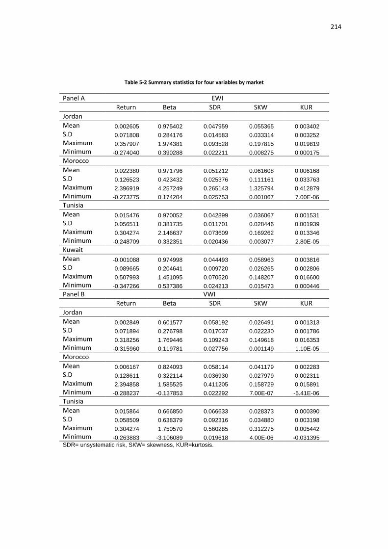
214
Table 5-2 Summary statistics for four variables by market
Panel A EWI
Return Beta SDR SKW KUR
Jordan
Mean 0.002605 0.975402 0.047959 0.055365 0.003402
S.D 0.071808 0.284176 0.014583 0.033314 0.003252
Maximum 0.357907 1.974381 0.093528 0.197815 0.019819
Minimum -0.274040 0.390288 0.022211 0.008275 0.000175
Morocco
Mean 0.022380 0.971796 0.051212 0.061608 0.006168
S.D 0.126523 0.423432 0.025376 0.111161 0.033763
Maximum 2.396919 4.257249 0.265143 1.325794 0.412879
Minimum -0.273775 0.174204 0.025753 0.001067 7.00E-06
Tunisia
Mean 0.015476 0.970052 0.042899 0.036067 0.001531
S.D 0.056511 0.381735 0.011701 0.028446 0.001939
Maximum 0.304274 2.146637 0.073609 0.169262 0.013346
Minimum -0.248709 0.332351 0.020436 0.003077 2.80E-05
Kuwait
Mean -0.001088 0.974998 0.044493 0.058963 0.003816
S.D 0.089665 0.204641 0.009720 0.026265 0.002806
Maximum 0.507993 1.451095 0.070520 0.148207 0.016600
Minimum -0.347266 0.537386 0.024213 0.015473 0.000446
Panel B VWI
Return Beta SDR SKW KUR
Jordan
Mean 0.002849 0.601577 0.058192 0.026491 0.001313
S.D 0.071894 0.276798 0.017037 0.022230 0.001786
Maximum 0.318256 1.769446 0.109243 0.149618 0.016353
Minimum -0.315960 0.119781 0.027756 0.001149 1.10E-05
Morocco
Mean 0.006167 0.824093 0.058114 0.041179 0.002283
S.D 0.128611 0.322114 0.036930 0.027979 0.002311
Maximum 2.394858 1.585525 0.411205 0.158729 0.015891
Minimum -0.288237 -0.137853 0.022292 7.00E-07 -5.41E-06
Tunisia
Mean 0.015864 0.666850 0.066633 0.028373 0.000390
S.D 0.058509 0.638379 0.092316 0.034880 0.003198
Maximum 0.304274 1.750570 0.560285 0.312275 0.005442
Minimum -0.263883 -3.106089 0.019618 4.00E-06 -0.031395
SDR= unsystematic risk, SKW= skewness, KUR=kurtosis.

215
and Morocco have lowest unsystematic risk (5.81%) and Tunisia has the highest
unsystematic risk (6.66%). Comparing unsystematic risk with returns, panel A of Table 5.2
shows that Morocco has the highest unsystematic risk and returns, whereas panel B of
Table 5.2 shows that Jordan has lowest unsystematic risk and returns and Tunisia has the
highest unsystematic risk and returns. Consequently, panels A and B of Table 5.2 show that
there is positive relationship between unsystematic risk and returns in Morocco using EWI
and Jordan and Tunisia using VWI.
For co-skewness, panel A of Table 5.2 shows that Morocco has the highest co-skewness
(6.16%) and Tunisia the lowest co-skewness (3.6%), while panel B of Table 5.2 indicates
that Morocco has highest co-skewness (4.1%) and Jordan lowest co-skewness (2.6%). The
relationship between co-skewness and return in panels A and B of Table 5.2 demonstrates
that county with highest co-skewness does not have lowest returns.
Finally, panels A and B of Table 5.2 report that Morocco has the highest co-kurtosis (0.06%)
and (0.02%) using EWI and VWI, respectively, while Tunisia has lowest co-kurtosis (0.015%)
and (0.003%) using EWI and VWI, respectively. Comparing co-kurtosis with returns in panel
A of Table 5.2 shows Morocco has the highest co-kurtosis and returns which implies there is
positive relationship between co-kurtosis and return in Morocco.
From the results of the descriptive analysis, initially it could be argued that the results of the
panel data regression show a positive relationship between beta and return for Jordan using
VWI, and a positive relationship between unsystematic risk and return in Morocco using EWI
and Jordan and Tunisia using VWI. There is no significant relationship between return and

216
co-skewness. Finally, there is a positive relationship between co-kurtosis and returns in
Morocco using EWI. To confirm or reject the preliminary results from descriptive analysis,
the following sub-sections will show the results of testing the unconditional relationship
between return and beta, unsystematic risk, co-skewness and co-kurtosis using panel data
regression.
5.2.3 The results of testing unconditional two-moment CAPM
The empirical results of an unconditional relationship between beta and return is
summarised in Tables 5.3 and 5.4. As a reminder, hypothesis1 assumes that the relationship
between beta and return is a positive. Investors would expect to earn a higher return when
they hold risky assets and vice versa when they hold less risky assets. However, the
empirical results obtained from Table 5. 3 show that the relationship between beta and
return is negative and insignificant in Jordan using pooled regression, and in Morocco using
three types of panel data regression. In Jordan a positive relationship exists between beta
and returns but it is insignificant using fixed and random regression, and this is also the case
in Tunisia and Kuwait using pooled, fixed and random regression. The findings reported in
Table 5.4 indicate that the relationship between beta and return is only significantly positive
in Jordan while in Morocco it is positive and insignificant, and negative and insignificant in
Tunisia. Based on these results the first hypothesis is rejected.
These results are associated with the results of the summary statistics which represented
prior sub-section and with the results of previous studies that found there is no statistically
significant relationship between beta and return, among them, Jacob (1971), Blume and

217
Friend (1973), Banz (1981), Hawawini et al (1983), Lakonishok and Shapiro (1986), Tinic
and West (1986), Carroll and Wei (1988), Wong and Tan (1991), Cheung and Wong (1992),
Fama and French (1992, 1996, 2004) and Cheung et al (1993). However, the results
obtained from Tables 5. 2 and 5.3 are inconsistent with the results of Jensen (1969), Black
et al (1972), Fama and McBeth (1973), Modigliani et al (1973) and Lau et al (1974),
Jahankhani (1976), Kothari et al (1995) and Strong and Xu(1997), who found a significant
positive relationship between beta and return.
The explanation for an absence of such a relationship between beta and return is that the
theory of CAPM relies on an expectation: that the expected market return is greater than the
return on risk-free asset, but this study and prior empirical studies of the CAPM have usually
been carried out by utilising realised market return, which may fall below the return on risk-
free asset to proxy for expected market return, in this situation there would not be a positive
relationship between beta and return. Moreover, the results reported in Tables 5.3 and 5.4
indicate that the relationship between beta and return in Jordan is sensitive to the choice of
market return index. Finally, low R-squares shown in Tables 5.3 and 5.4 suggest that there
might be additional risk factors other than beta which explain the relationship between risk
and return, this will be verified in the following sub-sections which will add additional risk
factors to beta; namely unsystematic risk, co-skewness and co-kurtosis.
5.2.4 The results of testing unsystematic risk
Tables 5.5 and 5.6 present the results of testing hypothesis 2, which states that investors are
compensated for unsystematic risk. The justification beyond this hypothesis is that CAPM

218
assumes that all investors hold a market portfolio that contains all assets in the market,
based on this assumption all investors hold diversifiable portfolio which allows them to avoid
unsystematic risk, and they demand a return compensation for bearing systematic risk which
cannot be avoided by diversification. In reality, investors may not hold market portfolio. For
instance, Goetzmann and Kumar’s (2004) surveyed sample contains more than 62,000
investors in the period from 1991 to 1996, and found that more than (25%) of investors’
portfolios contained only one stock, over half of investors’ portfolios contained no more than
three stocks, and less than 10% of the sample had portfolios containing more than ten
stocks. As a consequence, researchers like Bali , Cakici and Levy (2008), Ang et al,
Hodrick, Xing and Zhang (2009) and Fu (2009) relaxed the assumption that investors hold
market portfolio which is diversifiable, and they assumed that investors are compensated for
bearing unsystematic risk. Therefore, unsystematic risk is positively related to the cross
section of expected returns.
However, the results, reported in Table 5.5, show that the T-statistics for beta are
insignificant in four countries, and similar results are reported in Table 5.3. This also shows
that there is no statistically significant positive relationship between unsystematic risk and
return. By contrast, the results presented in Table 5.6 indicate that T- statistics for beta is
statistically significant in Jordan and insignificant in Morocco and Tunisia. Furthermore,
Table 5.6 indicates that T-statistics for unsystematic risk is significant for Jordan only, but as
a negative.
The results suggest that there may be no significant relationship between unsystematic risk,
as investors in four Arab stock markets hold well-diversified portfolios. Moreover, these
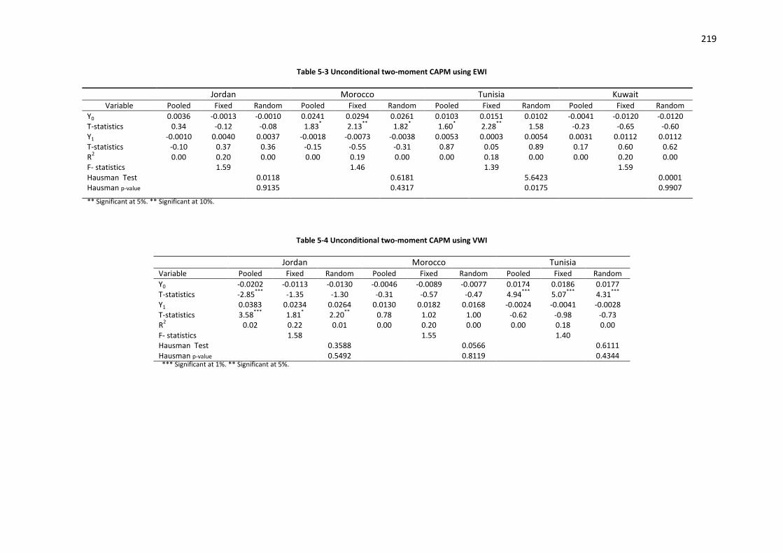
219
Table 5-3 Unconditional two-moment CAPM using EWI
Jordan Morocco Tunisia Kuwait Variable Pooled Fixed Random Pooled Fixed Random Pooled Fixed Random Pooled Fixed Random
Y0 0.0036 -0.0013 -0.0010 0.0241 0.0294 0.0261 0.0103 0.0151 0.0102 -0.0041 -0.0120 -0.0120 T-statistics 0.34 -0.12 -0.08 1.83
* 2.13
** 1.82
* 1.60
* 2.28
** 1.58
-0.23 -0.65 -0.60
Y1 -0.0010 0.0040 0.0037 -0.0018 -0.0073 -0.0038 0.0053 0.0003 0.0054 0.0031 0.0112 0.0112 T-statistics -0.10 0.37 0.36 -0.15 -0.55 -0.31 0.87 0.05 0.89 0.17 0.60 0.62 R
2 0.00 0.20 0.00 0.00 0.19 0.00 0.00 0.18 0.00 0.00 0.20 0.00
F- statistics 1.59 1.46 1.39 1.59 Hausman Test 0.0118 0.6181 5.6423 0.0001
Hausman p-value 0.9135 0.4317 0.0175 0.9907 ** Significant at 5%. ** Significant at 10%.
Table 5-4 Unconditional two-moment CAPM using VWI
Jordan Morocco Tunisia Variable Pooled Fixed Random Pooled Fixed Random Pooled Fixed Random
Y0 -0.0202 -0.0113 -0.0130 -0.0046 -0.0089 -0.0077 0.0174 0.0186 0.0177 T-statistics -2.85
*** -1.35 -1.30 -0.31 -0.57 -0.47 4.94
*** 5.07
*** 4.31
***
Y1 0.0383 0.0234 0.0264 0.0130 0.0182 0.0168 -0.0024 -0.0041 -0.0028 T-statistics 3.58
*** 1.81
* 2.20
** 0.78 1.02 1.00 -0.62 -0.98 -0.73
R2 0.02 0.22 0.01 0.00 0.20 0.00 0.00 0.18 0.00
F- statistics 1.58 1.55 1.40 Hausman Test 0.3588 0.0566 0.6111 Hausman p-value 0.5492 0.8119 0.4344 *** Significant at 1%. ** Significant at 5%.

220
Table 5-5 Unconditional two-moment CAPM with unsystematic risk using EWI
Table 5-6 Unconditional two-moment CAPM with unsystematic risk using VWI
Jordan Morocco Tunisia Kuwait
Variable Pooled Fixed Random Pooled Fixed Random Pooled Fixed Random Pooled Fixed Random
Y0 0.0005 -0.0008 -0.0016 0.0269 0.0295 0.0291 0.0082 0.0210 0.0074 -0.0108 0.0048 -0.0053 T-statistics 0.04 -0.07 -0.12 1.88
* 1.96
** 1.87
* 0.87 1.73
* 0.78 -0.46 0.18 -0.20
Y1 -0.0050 0.0047 0.0032 0.0017 -0.0072 -0.0005 0.0046 0.0015 0.0045 0.0018 0.0138 0.0121 T-statistics -0.40 0.35 0.25 0.12 -0.48 -0.03 0.70 0.22 0.68 0.10 0.73 0.66 Y2 0.1448 -0.0231 0.0232 -0.1210 -0.0021 -0.1232 0.0650 -0.1630 0.0879 0.1794 -0.4365 -0.1695 T-statistics 0.60 -0.09 0.09 -0.51 -0.01 -0.51 0.30 -0.58 0.41 0.46 -0.90 -0.39 R
2 0.00 0.20 0.00 0.00 0.19 0.00 0.00 0.18 0.00 0.00 0.20 0.00
F- statistics 1.58 1.45 1.39 1.59 Hausman Test 0.3325 3.1980 5.8645 1.6374 Hausman p-value 0.8468 0.2021 0.0533 0.4410 ** Significant at 5%* Significant at 10%.
Jordan Morocco Tunisia Variable Pooled Fixed Random Pooled Fixed Random Pooled Fixed Random
Y0 -0.0033 0.0064 0.0032 0.0069 -0.0014 0.0048 0.0231 0.0260 0.0238 T-statistics -0.28 0.46 0.23 0.41 -0.08 0.26 3.05
*** 3.34
*** 3.06
***
Y1 0.0421 0.0265 0.0299 0.0131 0.0183 0.0168 -0.0069 -0.0100 -0.0077 T-statistics 3.86
*** 2.02
** 2.43
*** 0.79 1.02 1.00 -1.04 -1.45 -1.17
Y2 -0.3293 -0.3342 -0.3151 -0.1986 -0.1284 -0.2141 -0.0387 -0.0515 -0.0420 T-statistics -1.86
* -1.57
-1.67
* -1.37 -0.81 -1.45 -0.84 -1.08 -0.92
R2 0.03 0.22 0.01 0.00 0.20 0.01 0.00 0.18 0.00
F- statistics 1.57 1.54 1.40 Hausman Test 0.5828 2.3866 1.1617 Hausman p-value 0.7472 0.3032 0.5594 ***significant at 1% **significant at 5% *significant at 10%

221
results are in agreement with the results of Hawawini et al (1983), Wong and Tan (1991),
Cheung and Wong (1992) and Cheung et al (1993) who found that the relationship between
unsystematic risk and return is insignificant. However, the results reported in Tables 5.5 and
5.6 are not associated with the results of the summary statistics shown in sub-section 5.2.2
and suggest that there is possibility that unsystematic risk is priced in some countries, and
with the results of recent studies provided by Bali and Cakici (2008) and Fu (2009) who
found a significant positive relationship between return and unsystematic risk. All results
summarised in Tables 5.3 to 5.6 show that fixed effects regression is not applicable; F-test
used to test significance of the model is insignificant at 0.1, 0.05 and 0.01 levels.
5.2.5 The results of testing unconditional three-moment CAPM
This sub-section presents the results of testing three-moment CAPM, which states that the
relationship between co-skewness and returns relies on the sign of market skewness.
Therefore, Table 5.7 shows the sign of market skewness for markets in sample study using
EWI and VWI respectively. As can be observed from Table 5.7 using EWI, Jordan and
Morocco have positive skewness while Tunisia and Kuwait have negative skewness. In
contrast, using VWI all countries have a positive skewness.
Table 5-7 Market skewness
EWI
Jordan Morocco Tunisia Kuwait
SKW 0.009571
1.457655
-0.33675
-0.28803
VWI
Jordan Morocco Tunisia SKW 0.233021
0.077754
0.371603

222
After, determining the sign of market skewness, Tables 5.8 and 5.9 show the results of the
tests of the relationship between return and co-skewness to see whether there is a
significant relationship with co-skewness, and the sign of this relationship is opposite to the
sign of market skewness.
As can be observed from Table 5.8, Jordan has statistically significant positive co-skewness
at 0.05 level, but not opposite to the market skewness. In addition, Table 5.8 shows that
Morocco only has significant negative co-skewness at 0.10 level, and it is opposite to the
sign of market skewness. However, Table 5.8 indicates that no country in the sample has a
significant positive relationship between beta and return; the results reported in Table 5.8 do
not support accepting a three-moment CAPM.
The findings summarised in Table 5.9 indicate that a three-moment CAPM is applicable in
Jordan only. The results that there is a significant relationship between return and co-
skewness for Morocco, as shown in Table 5.8, and for Jordan, as shown in Table 5.9, are
consistent with the theory of three-moment CAPM.
In general, the results reported in Tables 5.8 and 5.9 are not in accord with results of Kraus
and Litzenberger (1976) and Lim (1989) who found that the second and third moments are
priced. In contrast, results summarised in Tables 5.8 and 5.9 seem to support that results of
co-skewness do not play any role in explaining cores section returns, which were provided
by Friend and Westerfleld (1980), Hawawini et al (1983), Wong and Tan(1991), Cheung and
Wong (1992), Cheung et al (1993) and Vines et al (1994).

223
** Significant at 5%. * Significant at 10% .
Table 5-9 Unconditional three-moment CAPM using VWI
Table 5-8 Unconditional three-moment CAPM using EWI
Jordan Morocco Tunisia Kuwait Variable Pooled Fixed Random Pooled Fixed Random Pooled Fixed Random Pooled Fixed Random
Y0 0.0133 0.0548 0.0130 0.0030 0.0190 0.0069 0.0133 0.0070 0.0124 -0.0308 -0.0474 -0.0412 T-statistics 0.53 1.92
** 0.52 0.16 0.95 0.35 1.25 0.52 1.17 -1.21 -1.33 -1.30
Y1 -0.0209 -0.1084 -0.0200 0.0287 0.0078 0.0240 -0.0011 0.0177 0.0007 0.0604 0.0911 0.0767 T-statistics -0.44 -2.01
** -0.42 1.26 0.31 1.03 -0.06 0.68 0.04 1.43 1.28 1.33
Y2 0.1736 0.9670 0.1651 -0.1391 -0.0683 -0.1269 0.0918 -0.2416 0.0662 -0.4951 -0.7208 -0.5873 T-statistics 0.43 2.13
** 0.41 -1.60
* -0.72 -1.43 0.35 -0.69 0.26 -1.51
-1.17 -1.19
R2 0.00 0.21 0.00 0.00 0.19 0.00 0.00 0.18 0.00 0.00 0.20 0.00
F- statistics 1.65 1.43 1.39 1.57 Hausman Test 105.3936 3.4844 8.6950 0.1336 Hausman p-value 0.0000 0.1751 0.0129 0.9354
Jordan Morocco Tunisia Variable Pooled Fixed Random Pooled Fixed Random Pooled Fixed Random
Y0 -0.0464 -0.0361 -0.0426 0.0107 0.0061 0.0064 0.0203 0.0210 0.0205 T-statistics -4.85
*** -2.30
** -2.99
*** 0.58 0.30 0.32 4.36
*** 4.42
*** 3.91
***
Y1 0.1448 0.1077 0.1301 -0.0374 -0.0308 -0.0290 -0.0036 -0.0050 -0.0040 T-statistics 5.09
*** 2.29
** 3.36
*** -0.94 -0.64 -0.69 -0.89 -1.16 -0.99
Y2 -1.4274 -0.9753 -1.2381 0.6384 0.6175 0.5752 -0.0692 -0.0627 -0.0678 T-statistics -4.03
*** -1.87
* -2.81
*** 1.39 1.10 1.17 -0.93 -0.80 -0.91
R2 0.05 0.22 0.02 0.00 0.20 0.00 0.00 0.18 0.00
F- statistics 1.41
1.54
1.39 Hausman Test 1.1068 0.0943 0.4631
Hausman p-value 0.5750 0.9539 0.7933
** *Significant at 1%. ** Significant at 5%* Significant at 10%

224
5.2.6 The results of testing unconditional four-moment CAPM
Tables 5.10 and 5.11 present the results of an unconditional four-moment CAPM by using
EWI and VWI respectively. A four moment CAPM includes mean, co-variance, co-skewness
and co-kurtosis, states that the relationship between co-variance or beta, co-kurtosis and
return is positive. The relationship between co-skewness and return is positive (negative) if
market skewness is negative (positive). Thus, investors are compensated by higher
expected return for bearing beta and co-kurtosis. They forego the expected return for taking
the benefit of increasing the co-skewness.
As can be seen from Table 5.10 the four-moment CAPM is not applicable in all countries
included in the sample, and similar results are reported in Table 5.11. The result that beta,
co-skewness and co-kurtosis are not priced is contrary to evidence provided by Fang and
Lai (1997) who found that beta, co-skewness and co-kurtosis are determinants of the
expected excess rate of return. In addition, David and Chaudhry (2001) found that beta, co-
skewness and co-kurtosis moments are all important in explaining futures returns. Liow and
Chan (2005) found that higher moments are important in explaining real estate securities
and Doan et al (2010) who found that co-skewness and co-kurtosis in the US returns explain
15 and 17 of the 25 sub-portfolio returns respectively. Nevertheless, Chiao et al (2003),
Galagedera et al (2003) and Tang and Shum (2003, 2004) found that unconditional four-
moment CAPM perform poorly in explaining cross sectional security returns, which is in
accord with results reported in Tables 5.10 and 5.11, and with the results of descriptive
analysis that showed a weak relationship between returns and co-kurtosis.

225
Overall, the current section examines the performance of the unconditional four-moment
CAPM in four Arabic countries, namely Jordan, Morocco, Tunisia and Kuwait. Using EWI as
a proxy for the market portfolio, the results in Tables 5.3, 5.5, 5.8 and 5.10 reveal that four
hypotheses are rejected in four countries. The results reported in Tables 5.4, 5.6, 5.9 and
5.11 by using VWI as proxy for the market portfolio indicate that the first and third
hypotheses are not rejected in Jordan but are rejected in Morocco and Tunisia. The second
and fourth hypotheses are not accepted in all countries. Likewise, F-test and Hausman test
reported in Tables 5.3, 5.4, 5.5, 5.6, 5.8, 5.9, 5.10 and 5.11 indicate that fixed effects
regression is not appropriate. However, the thought of the low R –squares attributed to the
insufficient beta of a two moment CAPM to explain variation in stock returns does not find
any support by adding additional risk factors (unsystematic risk, co-skewness and co-
kurtosis).

226
Table 5-10 Unconditional four-moment CAPM using EWI
Table 5-11 Unconditional four-moment CAPM using VWI
Jordan Morocco Tunisia Variable Pooled Fixed Random Pooled Fixed Random Pooled Fixed Random Y0 -0.0438 -0.0190 -0.0357 0.0158 0.0061 0.0087 0.0195 0.0197 0.0195 T-statistics -4.22
*** -0.87 -2.01
** 0.82 0.28 0.41 3.74
*** 3.69
*** 3.30
***
Y1 0.1158 0.0067 0.0841 -0.0924 -0.0303 -0.0615 -0.0010 -0.0007 -0.0007 T-statistics 2.21
** 0.07 1.09 -1.23 -0.33 -0.75 -0.12 -0.07 -0.08
Y2 -0.4758 1.5995 0.0170 2.5088 0.5988 1.7113 -0.0928 -0.1043 -0.0994 T-statistics -0.32 0.69 0.01 1.13 0.22 0.72 -0.91 -0.92 -0.96 Y3 -7.9305 -18.7267 -9.4995 -16.1204 0.1576 -9.7812 -0.7015 -1.1891 -0.9291 T-statistics -0.66 -1.14 -0.68 -0.86 0.01 -0.50 -0.34 -0.51 -0.44 R
2 0.05 0.22 0.02 0.01 0.20 0.00 0.00 0.18 0.00
F- statistics 1.43 1.53 1.39 Hausman Test 1.8856 1.4258 0.5267 Hausman p-value 0.5965 0.6995 0.9130
*** Significant at 1%. ** Significant at 5%.
Jordan Morocco Tunisia Kuwait Variable Pooled Fixed Random Pooled Fixed Random Pooled Fixed Random Pooled Fixed Random
Y0 0.0002 0.0664 -0.0001 -0.0086 0.0139 -0.0041 0.0014 -0.0043 0.0005 -0.0315 -0.0102 -0.0010 T-statistics 0.01 1.36 0.00 -0.39 0.49 -0.17 0.09 -0.17 0.03 -0.90 -0.20 -0.02 Y1 0.0277 -0.1490 0.0285 0.0626 0.0220 0.0545 0.0411 0.0541 0.0433 0.0634 -0.0479 -0.0762 T-statistics 0.28 -1.00 0.29 1.51
0.36 1.18 0.89 0.76 0.95 0.58 -0.32 -0.62
Y2 -0.8270 1.7723 -0.8360 -0.6072 -0.2568 -0.5361 -1.2020 -1.2672 -1.2439 -0.5603 2.0081 2.5020 T-statistics -0.45 0.64 -0.46 -1.25 -0.34 -0.98 -0.92 -0.67 -0.96 -0.26 0.74 1.06 Y3 6.2046 -4.8795 6.2099 1.2181 0.4782 1.0517 11.4805 8.4817 11.6614 0.4234 -16.4049 -19.2152 T-statistics 0.56 -0.29 0.57 0.98 0.25 0.75 1.01 0.55 1.03 0.03 -1.04 -1.32 R
2 0.00 0.21 0.00 0.01 0.19 0.00 0.00 0.18 0.00 0.00 0.20 0.01
F- statistics 1.65 1.41 1.38 1.59 Hausman Test 93.6213 3.0439 10.5285 0.6588 Hausman p-value 0.0000 0.3849 0.0146 0.8829

227
5.3 Empirical results of testing conditional four- moment CAPM
The prior section examined unconditional four-moment CAPM, and it found that four
hypotheses that test the relationship between four independent variables (beta,
unsystematic risk, co-skewness and co-kurtosis) and return are rejected. Pettengill et al
(1995) pointed out that the explanation for the absence of a positive risk-return trade-off can
be attributed to the difference between the theory of the CAPM and the empirical tests that
examined CAPM. The theory of CAPM is based on expectations, it is built on expected
returns (ex-ante) are greater than the risk-free returns, while empirical tests are performed
by using realised returns (ex-post) which might be higher or lower than risk-free return. This
difference in used returns in theory and empirical tests of CAPM lead many empirical studies
to conclude that CAPM is not valid.
To overcome the problem of using realised returns instead of the expected returns, the
present section will adopt a conditional approach which relies on whether the sign of excess
market return is a positive or negative (realised returns is more (less) than risk-free return) to
test the relationship between four independent variables (beta, unsystematic risk, skewness
and kurtosis). Following Hodoshima et al (2000), this section will estimate separate
regressions, one when the market is up and the other when the market is down. It will be
divided into five sub-sections: the first sub-section presents summary statistics of variables,
the second sub-section presents the results of conditional two-moment CAPM, the third sub-
section presents the results of testing unsystematic risk, the fourth sub-section presents the
results of testing conditional three-moment CAPM, and the fifth sub-section presents the
results of conditional four-moment CAPM.

228
5.3.1 Summary statistics of variables
Tables 5.12 and 5.13 report summary statistics of four independent variables by market
using EWI and VWI respectively. Panel A in each table reports summary statistics when the
market is up and Panel B reports summary statistics when the market is down.
Panel A of Table 5.12 shows that the mean monthly return in all markets is positive and
ranges between (1.48%) Tunisia and (3.15%) Morocco. Additionally, Tunisia has the
smallest beta (28.3%) while Morocco has the highest beta (39%), and this reflects a positive
relationship between beta and return which is assumed by CAPM, because Tunisia also has
the smallest unsystematic risk (1.28%), co-skewness (1.06%) and co-kurtosis (0.047%) and
Morocco has the highest unsystematic risk (1.96%), co-skewness (2.077%) and co-kurtosis
(0.126%). It can be summarised that there exists a positive risk-return trade off.
Panel B of Table 5.12 shows that, with the exception of Tunisia which has a positive mean
monthly return, all other countries have a negative mean monthly return and positive beta,
unsystematic risk and co-kurtosis which supports view of there exists a negative relationship
between beta, unsystematic risk and co-kurtosis when market is down. From the data shown
in Panel B of Table 5.12, there is no obvious positive relationship between co-skewness and
return for all countries when the market is down.
From Table 5.13 Panel A, it can be observed that mean monthly return for countries is
positive and it ranges between (1.84%) Jordan and (1.32%) Tunisia. Morocco has the
highest beta which is close to the beta of Jordan and Tunisia has the lowest beta. In respect
to unsystematic risk Panel A shows that Jordan has the highest unsystematic risk (2.77%),

229
while Tunisia has the lowest unsystematic risk (1.55%). Similar to beta and unsystematic
risk, Tunisia has the lowest co-kurtosis (0.027%) and Morocco has the highest co-kurtosis
(0.082%). In general, Panel A of table 5.13 shows there is a positive relationship between
risk, which is measured by beta and unsystematic risk and co-kurtosis and return in an up
market.
With respect to co-skewness Panel A of Table 5.13 provides evidence against a negative
relationship existing between co-skewness and return when the market is up, with the
exception of Morocco. Panel A of Table 5.13 shows that Jordan has the highest co-
skewness and highest return, while Tunisia has lowest co-skewness and the lowest returns.
Except Tunisia, which has a positive mean monthly return in the down market, Panel B of
Table 5.13 shows that Jordan and Morocco have negative mean monthly return and positive
beta, unsystematic risk and co-kurtosis which confirms the assumption of there is a negative
relationship between return and beta, unsystematic risk and co-kurtosis when market is
down. As with Panel B of Table 5.12, Panel B of Table 5.13 shows no obvious positive
relationship between co-skewness and return for all countries when the market is down.
The explanation of a positive mean monthly return in the down market for Tunisia is a large
proportion of down months, where 70% of monthly observations of the excess market return
contain a negative excess market return, as shown in Table 5.14. Generally, the proportion
of down market is larger than the proportion of up market for all countries. These proportions
are inconsistent with the findings of Pettengill et al (1995), Fletcher (2000), Hodoshima et al
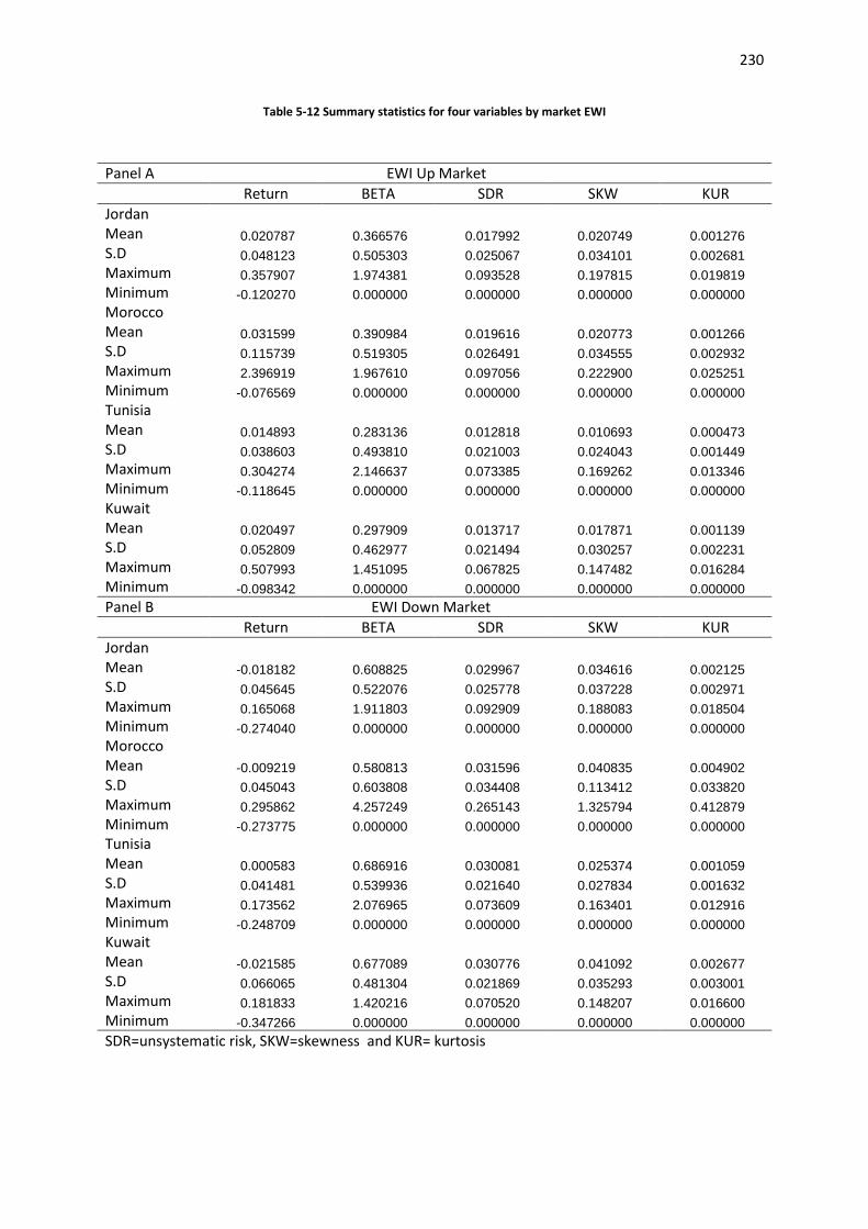
230
Table 5-12 Summary statistics for four variables by market EWI
Panel A EWI Up Market
Return BETA SDR SKW KUR
Jordan Mean 0.020787 0.366576 0.017992 0.020749 0.001276
S.D 0.048123 0.505303 0.025067 0.034101 0.002681
Maximum 0.357907 1.974381 0.093528 0.197815 0.019819
Minimum -0.120270 0.000000 0.000000 0.000000 0.000000
Morocco Mean 0.031599 0.390984 0.019616 0.020773 0.001266
S.D 0.115739 0.519305 0.026491 0.034555 0.002932
Maximum 2.396919 1.967610 0.097056 0.222900 0.025251
Minimum -0.076569 0.000000 0.000000 0.000000 0.000000
Tunisia Mean 0.014893 0.283136 0.012818 0.010693 0.000473
S.D 0.038603 0.493810 0.021003 0.024043 0.001449
Maximum 0.304274 2.146637 0.073385 0.169262 0.013346
Minimum -0.118645 0.000000 0.000000 0.000000 0.000000
Kuwait Mean 0.020497 0.297909 0.013717 0.017871 0.001139
S.D 0.052809 0.462977 0.021494 0.030257 0.002231
Maximum 0.507993 1.451095 0.067825 0.147482 0.016284
Minimum -0.098342 0.000000 0.000000 0.000000 0.000000
Panel B EWI Down Market
Return BETA SDR SKW KUR
Jordan Mean -0.018182 0.608825 0.029967 0.034616 0.002125
S.D 0.045645 0.522076 0.025778 0.037228 0.002971
Maximum 0.165068 1.911803 0.092909 0.188083 0.018504
Minimum -0.274040 0.000000 0.000000 0.000000 0.000000
Morocco Mean -0.009219 0.580813 0.031596 0.040835 0.004902
S.D 0.045043 0.603808 0.034408 0.113412 0.033820
Maximum 0.295862 4.257249 0.265143 1.325794 0.412879
Minimum -0.273775 0.000000 0.000000 0.000000 0.000000
Tunisia Mean 0.000583 0.686916 0.030081 0.025374 0.001059
S.D 0.041481 0.539936 0.021640 0.027834 0.001632
Maximum 0.173562 2.076965 0.073609 0.163401 0.012916
Minimum -0.248709 0.000000 0.000000 0.000000 0.000000
Kuwait Mean -0.021585 0.677089 0.030776 0.041092 0.002677
S.D 0.066065 0.481304 0.021869 0.035293 0.003001
Maximum 0.181833 1.420216 0.070520 0.148207 0.016600
Minimum -0.347266 0.000000 0.000000 0.000000 0.000000
SDR=unsystematic risk, SKW=skewness and KUR= kurtosis

231
(2000), Galagedera et al (2003), Ho et al (2006), Morelli (2007) and Lam and Li (2008) who
found that the proportion of up market is larger than the proportion of down market. These
are consistent with the findings of Theriou et al (2010) who found that the proportion of down
market is larger than the proportion of up market. The increase in this proportion had a
negative effect on one of two conditions which are required to test conditional CAPM; this
Table 5-13 Summary statistics for four variables by market VWI
Panel A VWI Up Market
Return BETA SDR SKW KUR
Jordan Mean 0.018427 0.308187 0.027792 0.013366 0.000650
S.D 0.051572 0.386736 0.031931 0.021605 0.001476
Maximum 0.318256 1.769446 0.108016 0.149618 0.016353
Minimum -0.184062 0.000000 0.000000 0.000000 0.000000
Morocco Mean 0.016508 0.322035 0.021703 14600.71 0.000829
S.D 0.058178 0.442202 0.030339 350416.7 0.001601
Maximum 0.690434 1.490788 0.113241 8410000. 0.009831
Minimum -0.173887 0.000000 0.000000 0.000000 -5.41E-06
Tunisia Mean 0.013251 0.228849 0.015541 0.007259 0.000274
S.D 0.037565 0.409982 0.037121 0.017254 0.000915
Maximum 0.236345 2.303949 0.557051 0.181586 0.014312
Minimum -0.225059 0.000000 0.000000 0.000000 0.000000
Panel B VWI Down Market
Return BETA SDR SKW KUR
Jordan Mean -0.015578 0.293390 0.030400 0.013124 0.000663
S.D 0.043976 0.328945 0.031039 0.019464 0.001370
Maximum 0.216657 1.764987 0.109243 0.136156 0.014103
Minimum -0.315960 0.000000 0.000000 0.000000 0.000000
Morocco Mean -0.010341 0.504951 0.036411 121527.8 0.001454
S.D 0.113199 0.478769 0.045018 2916667. 0.002279
Maximum 2.394858 1.585525 0.411205 70000000 0.015891
Minimum -0.288237 0.000000 0.000000 0.000000 -1.71E-06
Tunisia Mean 0.002613 0.587915 0.051092 0.021113 0.000965
S.D 0.045624 0.534974 0.093461 0.035014 0.002921
Maximum 0.304274 3.106089 0.560285 0.312275 0.031395
Minimum -0.263883 0.000000 0.000000 0.000000 0.000000
SDR=unsystematic risk, SKW=skewness and KUR= kurtosis

232
condition is that excess market return should be positive on average. Panel A of Table 5.15
shows that average excess market return is a negative in Kuwait, whereas Panel B of this
table shows that Morocco and Tunisia have a negative average excess market return. These
results are inconsistent with the findings of Pettengill et al (1995) who found that the excess
market return is positive on average. Thus, the existence of this negative average return has
an impact on the conditional relationship between risk and return, the results of which are
summarised in Tables 5.16 to 5.24.
Table 5-14 Proportions of up and down market months
Table 5-15 Average market excess returns
Overall, from the results of the summary statistics presented in Tables 5.12 and 5.13, one
can argue that the results of panel data regression may show a strong conditional
Panel A EWI
UP DOWN
Jordan 37.5% 62.5% Morocco 40% 60% Tunisia 30% 70% Kuwait 31% 69%
Panel B VWI
UP DOWN
Jordan 47% 53% Morocco 40% 60% Tunisia 30% 70%
Panel A EWI
Mean T-test
Jordan 0.0028 0.448 Morocco 0.0226 2.904***
Tunisia 0.0154 4.078***
Kuwait -0.0342 -3.810***
Panel B VWI
Mean T-test
Jordan 0.0134 1.449 Morocco -0.0142 -2.030***
Tunisia -0.0123 -2.999***

233
relationship between beta, unsystematic risk, co-kurtosis and returns. To confirm or reject
the preliminary results from the descriptive analysis, the following sub-sections will show the
results of testing conditional relationship between return and beta, unsystematic risk, co-
skewness and co-kurtosis using panel data regression.
5.3.2 The results of testing conditional two-moment CAPM
Tables 5.16 and 5.17 report the results of the conditional relationship between beta and
return using EWI and VWI, respectively. As can be seen from Tables 5.16 and 5.17, the
dual hypothesis which is related to the existence of a positive relationship between beta and
return in an up market and a negative relationship between beta and return in a down market
cannot be rejected at 0.01 level for three types of regression. These results imply that
portfolios with high beta earn higher return than portfolios with low beta in periods when
market is up (a positive relationship), while in periods when a market is down portfolios with
high beta receive lower return than portfolios with low beta (a negative relationship).
The findings reported in Tables 5.16 and 5.17 are consistent with many previous studies that
tested conditional CAPM among them Pettengill et al (1995, 2002), Fletcher (1997, 2000),
Howton and Peterson (1998), Isakov (1999), Hodoshima et al (2000), Crombez and Vennet
(2000), Faff (2001), Lam (2001), Tang and Shum(2003), Elsas et al (2003), Sandoval and
Saens (2004), Zhang and Wihlborg (2004), Ho et al (2006), Morelli (2007) and Theriou et al
(2010). However, all the above mentioned studies utilised cross section regression, while the
current study utilises panel regression.

234
Using a conditional approach to test CAPM, the value of R-squares becomes higher than it
was when an unconditional approach was used. This indicates an increased explanatory
power of model. F-test and Hausman tests reported in Tables 5.16 and 5.17 indicate that
fixed effects regression is not appropriate.
Pettengill et al (1995) stated that two conditions must be met for a positive relationship
between risk and return; the first condition is that market excess return on average should be
positive. The results of this condition are reported in Table 5.15 in the previous sub-section
and indicate that the average excess market return is negative in Kuwait using EWI and in
Morocco and Tunisia using VWI. The second condition is a symmetrical relationship
between risk and return in periods of up and down markets. A two-population T test was
used to test the second condition and the last row in Tables 5.16 and 5.17 presents the
results of testing the second condition and indicates a symmetrical relationship between beta
and return in up and down markets. These results are consistent with results of Pettengill et
al (1995) and Morelli (2007), but different to Fletcher (1997), who found an asymmetrical
relationship between beta and return in up and down markets. More specifically, Tables 5.16
and 5.17 show that the relationship between beta and return is stronger in an up market than
in a down market, which is considered inconsistent with the results of Pettengill et al (1995),
Fletcher (1997), Hodoshima et al (2000) and Lau, Lee and Mclnish (2002), who found that
the relationship between beta and return was stronger in a down market than in an up
market. However, it is considered consistent with the results of Fletcher (2000) and Tang
and Shum (2003) who found that the relationship between beta and return is stronger in a up
market than in an down market.

235
Table 5-16 Conditional two-moment CAPM using EWI
UP(EWI) Jordan Morocco Tunisia Kuwait Variable Pooled Fixed Random Pooled Fixed Random Pooled Fixed Random Pooled Fixed Random
Y0UP -0.0265 -0.0241 -0.0265 -0.0104 -0.0070 -0.0103 0.0026 0.0035 0.0027 -0.0300 -0.0294 -0.0297 T-statistics -8.66
*** -7.50
*** -8.66
*** -1.67
* -1.03 -1.49 1.03 1.37 1.00 -7.78
*** -7.31
*** -3.81
***
Y1UP 0.0795 0.0729 0.0795 0.0838 0.0751 0.0837 0.0456 0.0424 0.0452 0.0969 0.0951 0.0960 T-statistics 16.18
*** 13.11
*** 16.18
*** 8.77
*** 6.27
*** 8.64
*** 10.41
*** 8.80
*** 10.36
*** 13.84
*** 11.59
*** 13.51
***
R2 0.31 0.41 0.31 0.12 0.25 0.12 0.16 0.29 0.16 0.25 0.37 0.24
F- statistics 0.99 1.08 1.19 1.21 Hausman Test 6.5970 1.4773 1.8721 0.0518 Hausman p-value 0.0102 0.2242 0.1712 0.8199
DOWN(EWI) Jordan Morocco Tunisia Kuwait Variable Pooled Fixed Random Pooled Fixed Random Pooled Fixed Random Pooled Fixed Random
Y0DOWN 0.0481 0.0446 0.0472 0.0589 0.0538 0.0585 0.0399 0.0381 0.0395 0.0592 0.0582 0.0590 T-statistics 12.46
*** 10.62
*** 10.36
*** 8.43
*** 7.10
*** 7.00
*** 11.10
*** 10.34
*** 9.17
*** 10.44
*** 9.13
*** 6.65
***
Y1DOWN -0.0748 -0.0690 -0.0732 -0.0629 -0.0541 -0.0621 -0.0355 -0.0330 -0.0350 -0.0891 -0.0876 -0.0888 T-statistics -15.53
*** -12.48
*** -15.01
*** -7.53
*** -5.50
*** -7.34
*** -8.64
*** -7.60
*** -8.54
*** -13.04
*** -10.81
*** -12.65
***
R2 0.30 0.39 0.28 0.09 0.23 0.09 0.11 0.27 0.11 0.23 0.35 0.22
F- statistics 0.99 1.18 1.31 1.21 Hausman Test 2.5339 2.5705 2.1324 0.0905 Hausman p-value 0.1114 0.1089 0.1442 0.7635 Y0-U-Y0D=0 -3.50
*** -8.80
*** -7.30
*** 1.13
Y1-U-Y1D=0 0.32 1.23 1.73 -0.61
***significant at 1% *significant at 10%

236
Table 5-17 Conditional two-moment CAPM using VWI
Up(VWI) Jordan Morocco Tunisia Variable Pooled Fixed Random Pooled Fixed Random Pooled Fixed Random
Y0UP -0.0242 -0.0263 -0.0252 -0.0130 -0.0090 -0.0137 0.0065 0.0074 0.0067 T-statistics -7.15
*** -7.17
*** -4.23
*** -2.01
** -1.33 -1.40 2.44
*** 2.65
*** 2.33
**
Y1UP 0.0877 0.0946 0.0910 0.0596 0.0472 0.0616 0.0408 0.0369 0.0403 T-statistics 12.82
*** 11.12
*** 12.05
*** 5.02
*** 3.41
*** 5.03
*** 7.15
*** 5.34
*** 7.01
***
R2 0.22 0.37 0.20 0.04 0.21 0.04 0.08 0.22 0.08
F- statistics 1.47 1.39 1.16 Hausman Test 0.8450 4.8918 0.7746 Hausman p-value 0.3580 0.0270 0.3788
Down(VWI) Jordan Morocco Tunisia Variable Pooled Fixed Random Pooled Fixed Random Pooled Fixed Random
Y0DOWN 0.0305 0.0305 0.0303 0.0289 0.0217 0.0288 0.0318 0.0291 0.0314 T-statistics 8.39
*** 8.11
*** 4.17
*** 3.76
*** 2.62
*** 2.73
*** 9.04
*** 7.75
*** 8.63
***
Y1DOWN -0.0941 -0.0944 -0.0934 -0.0451 -0.0308 -0.0448 -0.0271 -0.0226 -0.0265 T-statistics -11.43
*** -10.18
*** -11.04
*** -4.08
*** -2.39
*** -3.89
*** -6.12
*** -4.50
*** -5.99
***
R2 0.19 0.35 0.17 0.03 0.20 0.03 0.06 0.21 0.06
F- statistics 1.58 1.41 1.21 Hausman Test 0.0650 5.8763 2.7241 Hausman p-value 0.7988 0.0153 0.0988 Y0-U-Y0D=0 -0.95 -1.97
* -3.04
**
Y1-U-Y1D=0 -0.11 0.65 0.51
*** Significant at 1%. ** Significant at 5%. * Significant at 10%.

237
5.3.3 The results of testing conditional unsystematic risk
Tables 5.18 and 5.19 report the results of testing the second hypothesis which relies on the
idea that investors do not hold market portfolio but hold only a few securities, which means
that investors do not hold an efficient and diversified portfolio; thus meaning unsystematic
risk related to company is important for them. As result, the second hypothesis states that
there exists a positive (negative) relationship between unsystematic risk and return in up
(down) markets, respectively. The results of using EWI in Table 5.18 show that the
relationship between unsystematic risk and return is significantly positive during periods
when the market is up at 0.01 level in all countries and significantly negative during periods
when the market is down at 0.01 level in all countries except in Morocco. Furthermore, the
results indicate that investors are compensated for bearing unsystematic risk. Using VWI,
Panel A of Table 5.19 shows that unsystematic risk is only significantly positive in Jordan,
while in Panel B of Table 5.19 it is significantly negative in all countries. Moreover, the
results reported in Table 5.18 using EWI are in line with results of Tang and Shum (2003,
2004 and 2006) who found that unsystematic risk is priced.
As can be observed from both tables, beta is significantly positive (negative) in up (down)
markets even when unsystematic risk is introduced, except in Tunisia in an up market when
EWI was used.

238
Table 5-18 Conditional two-moment CAPM with unsystematic risk using EWI
*** Significant at 1%. ** Significant at 5%. * Significant at 10%.
Up(EWI) Jordan Morocco Tunisia Kuwait Variable Pooled Fixed Random Pooled Fixed Random Pooled Fixed Random Pooled Fixed Random
Y0UP -0.0272 -0.0247 -0.0272 -0.0134 -0.0114 -0.0133 0.0009 0.0014 0.0010 -0.0306 -0.0302 -0.0304 T-statistics -8.88
*** 7.66
*** -8.88
*** 2.14
** -1.65
* 1.98
** 0.38 0.53 0.39 -7.96
*** -7.49
*** -3.60
***
Y1UP 0.0433 0.0466 0.0433 0.0437 0.0374 0.0436 0.0151 0.0110 0.0147 0.0443 0.0498 0.0436 T-statistics 2.91
*** 2.87
*** 2.91
*** 2.60
*** 2.08
** 2.60
*** 1.54
1.08 1.51
1.94
** 2.02
** 1.91
**
Y2UP 0.7736 0.5694 0.7736 0.9518 0.9788 0.9512 0.8009 0.8565 0.8020 1.1887 1.0417 1.1881 T-statistics 2.58
*** 1.72
* 2.58
*** 2.89
*** 2.82
*** 2.89
*** 3.47
*** 3.46
*** 3.50
*** 2.42
*** 1.94
** 2.41
***
R2 0.32 0.41 0.32 0.13 0.26 0.13 0.18 0.31 0.18 0.26 0.37 0.25
F- statistics 0.94 1.08 1.21 1.18 Hausman Test 6.4977 0.9907 1.6569 0.4911 Hausman p-value 0.0388 0.6094 0.4367 0.7823
Down(EWI) Jordan Morocco Tunisia Kuwait Variable Pooled Fixed Random Pooled Fixed Random Pooled Fixed Random Pooled Fixed Random Y0DOWN 0.0498 0.0461 0.0487 0.0601 0.0557 0.0599 0.0465 0.0454 0.0463 0.0634 0.0635 0.0635 T-statistics 12.78
*** 10.88
*** 10.09
*** 8.54
*** 7.19
*** 8.34
*** 12.40
*** 11.57
*** 9.99
*** 11.07
*** 9.94
*** 6.93
***
Y1DOWN -0.0479 -0.0431 -0.0439 -0.0449 -0.0382 -0.0451 -0.0054 -0.0041 -0.0045 -0.0417 -0.0270 -0.0298 T-statistics -4.20
*** -3.40
*** -3.79
*** -2.82
*** -2.27
*** -2.83
*** -0.76 -0.55 -0.62 -2.86
*** -1.65
* -1.99
**
Y2DOWN -0.6005 -0.5756 -0.6453 -0.3698 -0.3516 -0.3578 -0.9066 -0.8998 -0.9232 -1.1766 -1.5062 -1.4443 T-statistics -2.60
*** -2.26
** -2.76
*** -1.32 -1.16 -1.28 -5.08
*** -4.72
*** -5.12
*** -3.67
*** -4.25
*** -4.44
***
R2 0.30 0.40 0.29 0.09 0.23 0.09 0.15 0.30 0.15 0.25 0.37 0.24
F- statistics 0.98 1.18 1.31 1.30 Hausman Test 2.7533 2.3796 0.6565 0.2117 Hausman p-value 0.2524 0.3043 0.7202 0.8996 Y0-U-Y0D=0 -4.61
*** -9.92
*** -9.92
*** -1.00
Y1-U-Y1D=0 0.70 0.80 1.42 1.19 Y2U-Y2D=0 0.74 0.95 1.00 -0.88
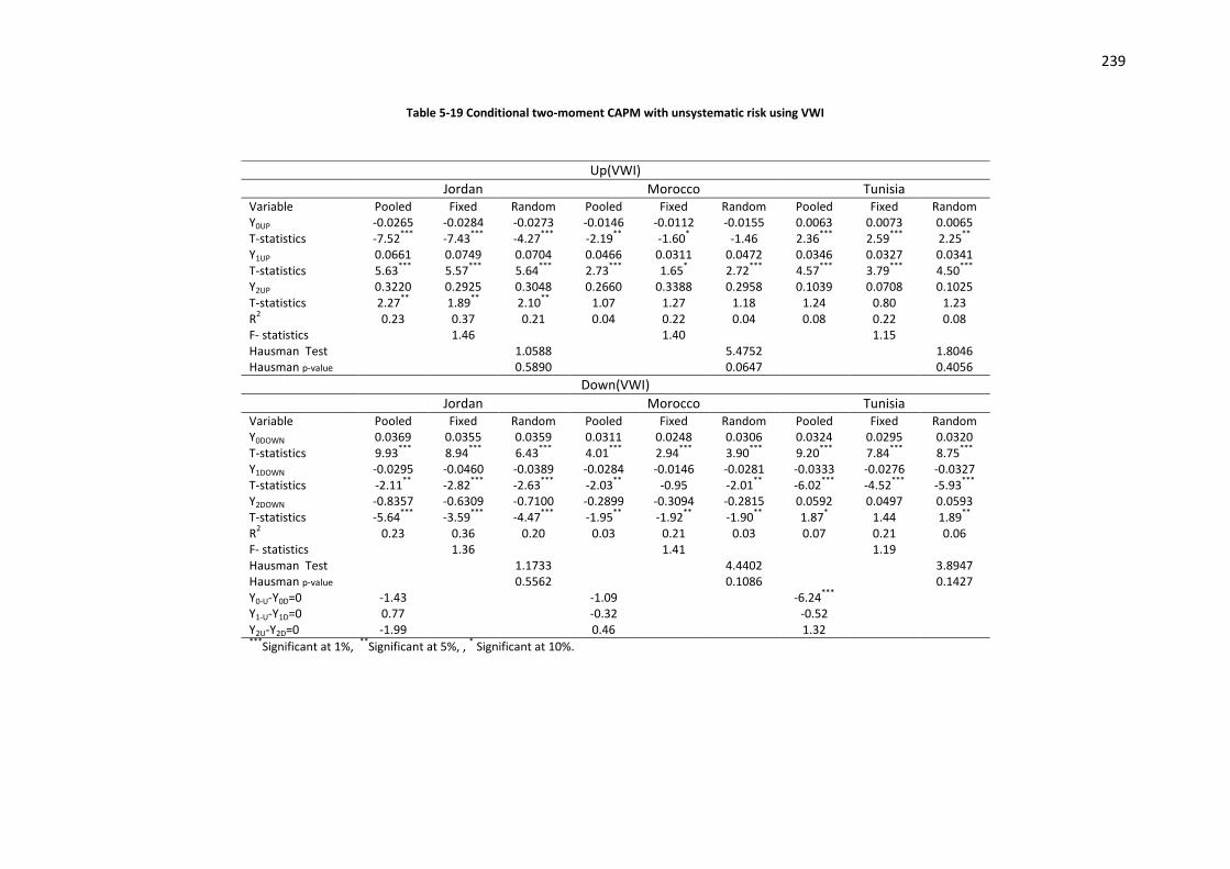
239
Table 5-19 Conditional two-moment CAPM with unsystematic risk using VWI
Up(VWI) Jordan Morocco Tunisia Variable Pooled Fixed Random Pooled Fixed Random Pooled Fixed Random Y0UP -0.0265 -0.0284 -0.0273 -0.0146 -0.0112 -0.0155 0.0063 0.0073 0.0065 T-statistics -7.52
*** -7.43
*** -4.27
*** -2.19
** -1.60
* -1.46 2.36
*** 2.59
*** 2.25
**
Y1UP 0.0661 0.0749 0.0704 0.0466 0.0311 0.0472 0.0346 0.0327 0.0341 T-statistics 5.63
*** 5.57
*** 5.64
*** 2.73
*** 1.65
* 2.72
*** 4.57
*** 3.79
*** 4.50
***
Y2UP 0.3220 0.2925 0.3048 0.2660 0.3388 0.2958 0.1039 0.0708 0.1025 T-statistics 2.27
** 1.89
** 2.10
** 1.07 1.27 1.18 1.24 0.80 1.23
R2 0.23 0.37 0.21 0.04 0.22 0.04 0.08 0.22 0.08
F- statistics 1.46 1.40 1.15 Hausman Test 1.0588 5.4752 1.8046 Hausman p-value 0.5890 0.0647 0.4056
Down(VWI) Jordan Morocco Tunisia Variable Pooled Fixed Random Pooled Fixed Random Pooled Fixed Random Y0DOWN 0.0369 0.0355 0.0359 0.0311 0.0248 0.0306 0.0324 0.0295 0.0320 T-statistics 9.93
*** 8.94
*** 6.43
*** 4.01
*** 2.94
*** 3.90
*** 9.20
*** 7.84
*** 8.75
***
Y1DOWN -0.0295 -0.0460 -0.0389 -0.0284 -0.0146 -0.0281 -0.0333 -0.0276 -0.0327 T-statistics -2.11
** -2.82
*** -2.63
*** -2.03
** -0.95 -2.01
** -6.02
*** -4.52
*** -5.93
***
Y2DOWN -0.8357 -0.6309 -0.7100 -0.2899 -0.3094 -0.2815 0.0592 0.0497 0.0593 T-statistics -5.64
*** -3.59
*** -4.47
*** -1.95
** -1.92
** -1.90
** 1.87
* 1.44 1.89
**
R2 0.23 0.36 0.20 0.03 0.21 0.03 0.07 0.21 0.06
F- statistics 1.36 1.41 1.19 Hausman Test 1.1733 4.4402 3.8947 Hausman p-value 0.5562 0.1086 0.1427 Y0-U-Y0D=0 -1.43 -1.09 -6.24
***
Y1-U-Y1D=0 0.77 -0.32 -0.52 Y2U-Y2D=0 -1.99 0.46 1.32 ***
Significant at 1%, **
Significant at 5%, , * Significant at 10%.
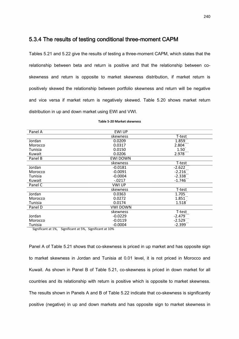
240
5.3.4 The results of testing conditional three-moment CAPM
Tables 5.21 and 5.22 give the results of testing a three-moment CAPM, which states that the
relationship between beta and return is positive and that the relationship between co-
skewness and return is opposite to market skewness distribution, if market return is
positively skewed the relationship between portfolio skewness and return will be negative
and vice versa if market return is negatively skewed. Table 5.20 shows market return
distribution in up and down market using EWI and VWI.
Table 5-20 Market skewness
Panel A of Table 5.21 shows that co-skewness is priced in up market and has opposite sign
to market skewness in Jordan and Tunisia at 0.01 level, it is not priced in Morocco and
Kuwait. As shown in Panel B of Table 5.21, co-skewness is priced in down market for all
countries and its relationship with return is positive which is opposite to market skewness.
The results shown in Panels A and B of Table 5.22 indicate that co-skewness is significantly
positive (negative) in up and down markets and has opposite sign to market skewness in
Panel A EWI UP skewness T-test Jordan 0.0209 1.859** Morocco 0.0317 2.804*** Tunisia 0.0150 1.50* Kuwait 0.0206 2.978*** Panel B EWI DOWN skewness T-test Jordan -0.0181 -2.622*** Morocco -0.0091 -2.216** Tunisia -0.0004 -2.338** Kuwait -.0217 -1.746** Panel C VWI UP skewness T-test Jordan 0.0363 1.705** Morocco 0.0272 1.851** Tunisia 0.0174 1.518* Panel D VWI DOWN skewness T-test Jordan -0.0229 -2.479*** Morocco -0.0119 -2.529*** Tunisia -0.0004 -2.399** ***
Significant at 1%, **
Significant at 5%, *Significant at 10%

241
Jordan and Tunisia, but for Morocco co-skewness is insignificant and has sign similar to
market skewness in up market, whereas in down market it is significant and its sign also is
similar to market skewness.
Tang and Shum (2003) pointed out that the significantly negative relationship between co-
skewness and returns in up markets means that investors accept/require smaller (larger)
portfolio returns for positively (negatively) skewed portfolios when the market excess returns
are positive. The significantly positive relationship between co-skewness and returns in
down markets means that the losses incurred are not so serious for positively skewed
portfolios when the market excess returns are negative.
In short, the null hypothesis of the three-moment CAPM which states that co-skewness is
not priced is rejected in Jordan and Tunisia using both EWI and VWI, and the results
strongly indicate that rational investors prefer positive skewness but demand compensation
(higher expected returns) for negative skewness (Tang and Shum, 2003). More importantly,
the relationship between beta and return in Tables 5.21 and 5.22 remains significantly
positive (negative) in up (down) markets even when co-skewness is introduced in
regression. Therefore, it can be stated that the third hypothesis which states that there is a
negative(positive) relationship between co- skewness and return in up (down) markets was
proved in Jordan and Tunisia.
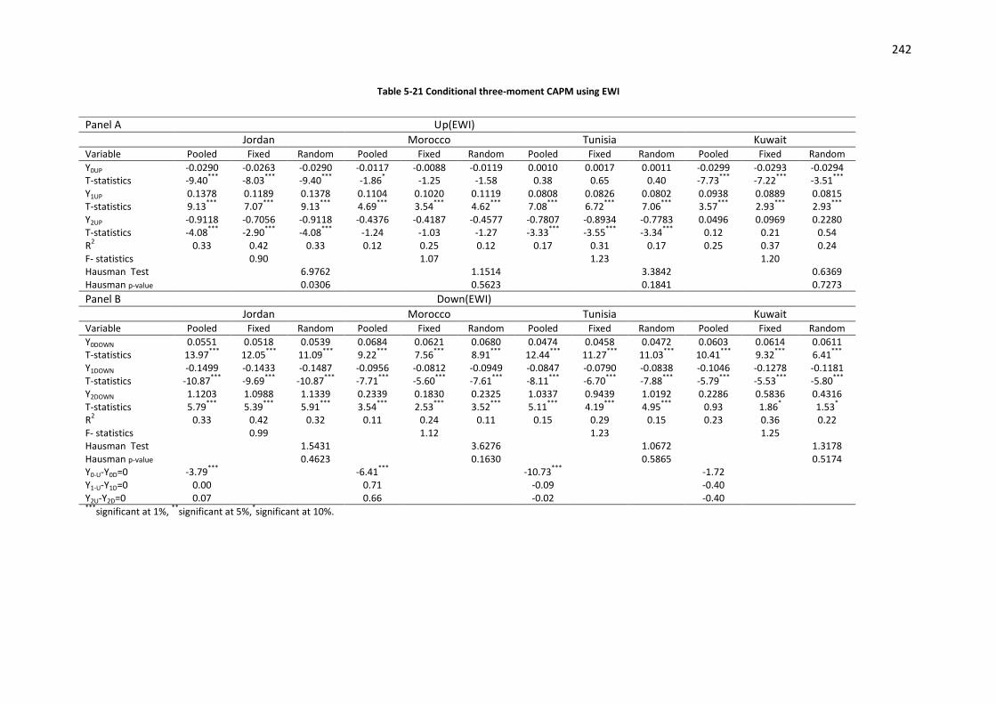
242
Table 5-21 Conditional three-moment CAPM using EWI
Panel A Up(EWI) Jordan Morocco Tunisia Kuwait Variable Pooled Fixed Random Pooled Fixed Random Pooled Fixed Random Pooled Fixed Random
Y0UP -0.0290 -0.0263 -0.0290 -0.0117 -0.0088 -0.0119 0.0010 0.0017 0.0011 -0.0299 -0.0293 -0.0294 T-statistics -9.40
*** -8.03
*** -9.40
*** -1.86
* -1.25 -1.58
0.38 0.65 0.40 -7.73
*** -7.22
*** -3.51
***
Y1UP 0.1378 0.1189 0.1378 0.1104 0.1020 0.1119 0.0808 0.0826 0.0802 0.0938 0.0889 0.0815 T-statistics 9.13
*** 7.07
*** 9.13
*** 4.69
*** 3.54
*** 4.62
*** 7.08
*** 6.72
*** 7.06
*** 3.57
*** 2.93
*** 2.93
***
Y2UP -0.9118 -0.7056 -0.9118 -0.4376 -0.4187 -0.4577 -0.7807 -0.8934 -0.7783 0.0496 0.0969 0.2280 T-statistics -4.08
*** -2.90
*** -4.08
*** -1.24 -1.03 -1.27 -3.33
*** -3.55
*** -3.34
*** 0.12 0.21 0.54
R2 0.33 0.42 0.33 0.12 0.25 0.12 0.17 0.31 0.17 0.25 0.37 0.24
F- statistics 0.90 1.07 1.23 1.20 Hausman Test 6.9762 1.1514 3.3842 0.6369 Hausman p-value 0.0306 0.5623 0.1841 0.7273
Panel B Down(EWI) Jordan Morocco Tunisia Kuwait Variable Pooled Fixed Random Pooled Fixed Random Pooled Fixed Random Pooled Fixed Random
Y0DOWN 0.0551 0.0518 0.0539 0.0684 0.0621 0.0680 0.0474 0.0458 0.0472 0.0603 0.0614 0.0611 T-statistics 13.97
*** 12.05
*** 11.09
*** 9.22
*** 7.56
*** 8.91
*** 12.44
*** 11.27
*** 11.03
*** 10.41
*** 9.32
*** 6.41
***
Y1DOWN -0.1499 -0.1433 -0.1487 -0.0956 -0.0812 -0.0949 -0.0847 -0.0790 -0.0838 -0.1046 -0.1278 -0.1181 T-statistics -10.87
*** -9.69
*** -10.87
*** -7.71
*** -5.60
*** -7.61
*** -8.11
*** -6.70
*** -7.88
*** -5.79
*** -5.53
*** -5.80
***
Y2DOWN 1.1203 1.0988 1.1339 0.2339 0.1830 0.2325 1.0337 0.9439 1.0192 0.2286 0.5836 0.4316 T-statistics 5.79
*** 5.39
*** 5.91
*** 3.54
*** 2.53
*** 3.52
*** 5.11
*** 4.19
*** 4.95
*** 0.93 1.86
* 1.53
*
R2 0.33 0.42 0.32 0.11 0.24 0.11 0.15 0.29 0.15 0.23 0.36 0.22
F- statistics 0.99 1.12 1.23 1.25 Hausman Test 1.5431 3.6276 1.0672 1.3178 Hausman p-value 0.4623 0.1630 0.5865 0.5174 Y0-U-Y0D=0 -3.79
*** -6.41
*** -10.73
*** -1.72
Y1-U-Y1D=0 0.00 0.71 -0.09 -0.40 Y2U-Y2D=0 0.07 0.66 -0.02 -0.40 ***
significant at 1%, **
significant at 5%,*significant at 10%.

243
Table 5-22 Conditional three-moment CAPM using VWI
Up(VWI) Jordan Morocco Tunisia Variable Pooled Fixed Random Pooled Fixed Random Pooled Fixed Random Y0UP -0.0267 -0.0307 -0.0287 -0.0132 -0.0094 -0.0139 0.0047 0.0052 0.0049 T-statistics -7.69
*** -7.84
*** -4.68
*** -2.03
** -1.38 -1.38 1.74
* 1.78
* 1.69
*
Y1UP 0.1370 0.1557 0.1464 0.0598 0.0479 0.0619 0.0837 0.0809 0.0826 T-statistics 7.47
*** 7.09
*** 7.42
*** 5.03
*** 3.45
*** 5.04
*** 5.74
*** 4.70
*** 5.65
***
Y2UP -0.9493 -1.0831 -1.0143 0.0000 0.0000 0.0000 -1.1065 -1.0760 -1.0890 T-statistics -2.89
*** -3.02
*** -3.03
*** 0.53 0.60 0.67 -3.19
*** -2.79
*** -3.14
***
R2 0.23 0.38 0.21 0.04 0.21 0.04 0.10 0.24 0.09
F- statistics 1.50 1.39 1.14 Hausman Test 2.0604 4.9202 0.1041 Hausman p-value 0.3569 0.0854 0.9493
Down(VWI) Jordan Morocco Tunisia Variable Pooled Fixed Random Pooled Fixed Random Pooled Fixed Random Y0DOWN 0.0338 0.0343 0.0333 0.0298 0.0227 0.0296 0.0393 0.0368 0.0390 T-statistics 8.98
*** 8.72
*** 4.79
*** 3.88
*** 2.73
*** 2.78
*** 10.14
*** 8.58
*** 9.73
***
Y1DOWN -0.1556 -0.1593 -0.1500 -0.0460 -0.0321 -0.0456 -0.0612 -0.0560 -0.0606 T-statistics -7.16
*** -6.87
*** -6.98
*** -4.17
*** -2.49
*** -3.96
*** -6.78
*** -5.29
*** -6.68
***
Y2DOWN 1.1216 1.1672 1.0309 0.0000 0.0000 0.0000 0.5958 0.5666 0.5926 T-statistics 3.05
*** 3.05
*** 2.86
*** -1.92
** -1.48 -1.82
* 4.32
*** 3.57
*** 4.29
***
R2 0.20 0.36 0.19 0.03 0.21 0.09 0.23 0.09
F- statistics 1.60 1.39 0.03 1.16 Hausman Test 1.1928 5.3764 1.6320 Hausman p-value 0.5508 0.0680 0.4422 Y0-U-Y0D=0 -1.43 -2.29
** -4.61
***
Y1-U-Y1D=0 -1.89* -1.34 0.75
Y2U-Y2D=0 -1.81 -0.42 0.79 ***
significant at 1%, **
significant at 5%,*significant at 10%.

244
The results of three-moment CAPM is held in Jordan and Tunisia are consistent with results
of Galagedera et al (2003) and Tang and Shum (2006) who found that the relationship
between beta and return is positive (negative) in up and (down) markets and relationship
between co-skewness and return is negative (positive) in up and (down) markets. The
results that co-skewness is significantly positive in down market for all countries using EWI
are consistent with findings of Hung et al (2004) who found that co-skewness is only priced
in down market. The result that co-skewness is not an important risk factor for Kuwait and
Morocco in up market is in line with the results of Tang and Shum (2004).
5.3.5 The results of testing conditional four-moment CAPM
Tables 5.23 and 5.24 give the results of the fourth hypothesis which tested the relationship
between return and co-kurtosis in addition to beta and co-skewness when the conditional
approach is introduced. Like beta, four-moment CAPM assumes that investors are
compensated for bearing co-kurtosis, and hence the relationship between co-kurtosis and
return is a positive in up market and negative in down market.
Panel A of Table 5.23 shows a significant positive relationship between beta and return
across all countries during periods when the market return is positive. Panel A of Table 5. 23
indicates that co-skewness is a significant negative in Jordan only. It also shows that co-
kurtosis is not found to be statistically significant across all countries. Contrary to the results
reported in Panel A, Panel B of Table 5.23 shows that beta and co-skewness are priced
across all countries. Co-skewness is found to be priced in Jordan when the market is up and
all countries when the market is down due to portfolio returns for Jordan being more skewed
245
when the market is up. For all countries portfolio returns are more skewed in a down market
than up. Although co-kurtosis is found to be priced in Tunisia and Kuwait, the explanation for
this phenomenon is the increased proportion of down market in Tunisia and Kuwait, where
Table 5.14 shows that Tunisia and Kuwait have a higher number of down market months.
From the above results it is clear that the fourth hypothesis, which states that there is a
positive (negative) relationship between co-kurtosis and return in an up (down) market, was
not rejected in Tunisia and Kuwait when the market is down. The results reported in Table
5.23 are inconsistent with the results of Chiao et al (2003) who found that beta, co-skewness
and co-kurtosis are significant in up markets.
Panel A of Table 5.24 indicates that beta, co-skewness and co-kurtosis as explanatory
variables in a four-moment CAPM are significant in Tunisia and their signs are consistent
with what was expected. For Jordan, beta and co-skewness only are found to be statistically
significant. For Morocco, beta is significant and positive as predicted. However, co-skewness
and co-kurtosis are insignificant and positive and negative respectively, opposite to the
prediction. Furthermore, Panel B of Table 5.24 shows that in Jordan and Tunisia the beta
and co-kurtosis is a significant negative and co-skewness is a positive which is consistent
with prediction of a four-moment CAPM. For Morocco, beta, co-skewness and co-kurtosis
are significant but co-skewness and co-kurtosis have sign opposite to as four-moments
predicts. In short, the first, second and third null hypotheses related to conditional four-
moment CAPM are rejected in Tunisia when the market is up or down, and in Jordan when
the market is down. The findings presented in both Tables 5.23 and 5.24 are not in
agreement with the findings of Galagedera et al (2003) who found that co-kurtosis is priced
in neither up and down markets.

246
Overall, the results reported in Tables 5.16 to 5.24 show the test of four hypotheses related
to four independent variables: beta, unsystematic risk, co-skewness, and co-kurtosis. The
results of Tables 5.16 and 5.17 confirm the first hypothesis, which tests the relationship
between beta and return in all countries. Table 5.18 shows that the second hypothesis,
which tests the relationship between unsystematic risk and return, was not rejected in
Jordan, Tunisia and Kuwait, while Table 5.19 shows that the second hypothesis was not
rejected in Jordan. With regards to the third hypothesis, which tests the relationship between
co-skewness and return, the results in Tables 5.21 and 5.22 show that this hypothesis was
not rejected in Jordan and Tunisia. Finally, the fourth hypothesis which tests the relationship
between co-kurtosis and return was not rejected in Tunisia, as Table 5.24 shows.

247
Table 5-23 Conditional four-moment CAPM using EWI
Panel A Up(EWI) Jordan Morocco Tunisia Kuwait Variable Pooled Fixed Random Pooled Fixed Random Pooled Fixed Random Pooled Fixed Random
Y0UP -0.0292 -0.0268 -0.0292 -0.0116 -0.0083 -0.0117 0.0008 0.0016 0.0010 -0.0301 -0.0296 -0.0295 T-statistics -9.45
*** -8.14
*** -9.45
*** -1.83
* -1.17 -1.45 0.33 0.63 0.35 -7.76
*** -7.25
*** -3.42
***
Y1UP 0.1824 0.1995 0.1824 0.0960 0.0693 0.0945 0.0912 0.0845 0.0897 0.1490 0.1420 0.1112 T-statistics 3.87
*** 3.68
*** 3.87
*** 1.75
* 1.09 1.66
* 3.38
*** 2.95
*** 3.34
*** 1.93
** 1.72
* 1.44
Y2UP -2.3431 -3.2928 -2.3431 0.0373 0.6398 0.1236 -1.2694 -0.9821 -1.2218 -1.6684 -1.5533 -0.7000 T-statistics -1.62
* -1.97
** -1.62
* 0.02 0.34 0.07 -1.09 -0.80 -1.05 -0.73 -0.64 -0.31
Y3UP 10.6414 19.2353 10.6414 -3.4654 -7.6889 -4.2660 5.0363 0.9191 4.5749 12.6699 12.2372 6.8743 T-statistics 1.00 1.57
1.00 -0.29 -0.58 -0.35 0.43 0.07 0.39 0.76 0.69 0.42
R2 0.33 0.42 0.33 0.12 0.25 0.12 0.18 0.31 0.17 0.25 0.37 0.24
F- statistics 0.92 1.07 1.20 Hausman Test 9.0847 1.4457 3.4070 1.6797 Hausman p-value 0.0282 0.6949 0.3330 0.6415
Panel B Down(EWI) Jordan Morocco Tunisia Kuwait Variable Pooled Fixed Random Pooled Fixed Random Pooled Fixed Random Pooled Fixed Random
Y0DOWN 0.0555 0.0521 0.0541 0.0703 0.0642 0.0700 0.0493 0.0475 0.0491 0.0621 0.0634 0.0629 T-statistics 14.01
*** 12.04
*** 10.58
*** 9.34
*** 7.61
*** 9.07
*** 12.59
*** 11.46
*** 11.14
*** 10.61
*** 9.58
*** 8.05
***
Y1DOWN -0.1866 -0.1695 -0.1834 -0.1320 -0.1140 -0.1303 -0.1220 -0.1172 -0.1218 -0.2001 -0.2470 -0.2466 T-statistics -5.14
*** -3.94
*** -4.80
*** -4.79
*** -3.40
*** -4.71
*** -5.76
*** -5.15
*** -5.74
*** -3.81
*** -4.44
*** -4.71
***
Y2DOWN 2.3346 1.9662 2.2844 0.9330 0.8020 0.9096 2.7519 2.7260 2.7736 3.0940 4.2575 4.3938 T-statistics 2.07
** 1.46 1.92
** 1.95
** 1.39 1.90
** 3.15
*** 2.91
*** 3.17
*** 2.06
** 2.67
*** 2.92
***
Y3DOWN -9.4503 -6.7363 -8.9188 -1.9227 -1.6930 -1.8608 -18.7241 -19.5794 -19.1583 -20.4655 -26.9514 -28.9585 T-statistics -1.09 -0.65 -0.98 -1.50
-1.08 -1.43 -2.02
** -1.96
** -2.07
** -1.94
** -2.35
*** -2.71
***
R2 0.34 0.42 0.32 0.11 0.24 0.11 0.16 0.30 0.16 0.23 0.36 0.23
F- statistics 0.98 1.10 1.24 1.28 Hausman Test 1.5989 1.3187 0.8891 Hausman p-value 0.6596 0.7247 0.8281 Y0-U-Y0D=0 -3.79
*** -5.63
*** -8.90
*** -1.51
Y1-U-Y1D=0 -0.52 0.98 0.42 -0.64 Y2U-Y2D=0 0.63 2.47
** 1.47 0.57
Y3U-Y3D=0 0.71 2.36**
1.66 1.17 ***
significant at 1%, **
significant at 5%,*significant at 10%.

248
Table 5-24 Conditional four-moment CAPM using VWI
Panel A Up(VWI) Jordan Morocco Tunisia Variable Pooled Fixed Random Pooled Fixed Random Pooled Fixed Random
Y0UP -0.0271 -0.0314 -0.0294 -0.0136 -0.0102 -0.0150 0.0041 0.0043 0.0042 T-statistics -7.77
*** -7.92
*** -4.93
*** -2.07
** -1.46 -1.53
1.52
1.47 1.39
Y1UP 0.1804 0.2031 0.2038 0.0678 0.0601 0.0799 0.1337 0.1392 0.1338 T-statistics 4.22
*** 4.35
*** 4.68
*** 2.95
*** 2.29
** 3.35
*** 4.73
*** 4.33
*** 4.71
***
Y2UP -2.6562 -2.9067 -3.2534 0.0000 0.0000 0.0000 -3.7946 -4.1441 -3.8175 T-statistics -1.71
** -1.79
** -2.11
** 0.54 0.60 0.67 -2.81
*** -2.80
*** -2.83
***
Y3UP 15.1504 16.1354 19.8419 -2.5686 -3.7764 -5.6220 31.7054 35.8858 32.0628 T-statistics 1.12 1.15 1.50
-0.41 -0.54 -0.87 2.06
** 2.15
** 2.08
**
R2 0.24 0.38 0.22 0.04 0.22 0.04 0.10 0.24 0.10
F- statistics 1.50 1.39 1.15 Hausman Test 4.0363 4.8672 0.4412 Hausman p-value 0.2576 0.1818 0.9316
Panel B Down(VWI) Jordan Morocco Tunisia Variable Pooled Fixed Random Pooled Fixed Random Pooled Fixed Random
Y0DOWN 0.0362 0.0356 0.0352 0.0353 0.0277 0.0344 0.0411 0.0392 0.0408 T-statistics 9.79
*** 9.18
*** 6.77
*** 4.50
*** 3.25
*** 3.07
*** 10.20
*** 8.38
*** 9.79
***
Y1DOWN -0.3944 -0.3456 -0.3691 -0.0904 -0.0719 -0.0871 -0.0888 -0.0823 -0.0872 T-statistics -8.25
*** -6.88
*** -7.72
*** -4.95
*** -3.49
*** -4.68
*** -4.63
*** -3.50
*** -4.53
***
Y2DOWN 10.5146 8.5786 9.6745 0.0000 0.0000 0.0000 1.6933 1.5632 1.6505 T-statistics 6.10
*** 4.71
*** 5.58
*** -1.98
** -1.49 -1.86
** 2.46
*** 1.93
** 2.40
***
Y3DOWN -83.8426 -66.3240 -77.0087 11.6365 10.4159 11.1118 -9.1606 -8.1861 -8.8216 T-statistics -5.57
*** -4.16
*** -5.08
*** 3.03
*** 2.47
*** 2.84
*** -1.63
* -1.25 -1.57
R2 0.24 0.38 0.22 0.05 0.22 0.04 0.10 0.23 0.09
F- statistics 1.45 1.36 1.14 Hausman Test 4.9780 4.8396 0.9751 Hausman p-value 0.1734 0.1839 0.8073 Y0-U-Y0D=0 -1.43 -2.52
** -5.68
***
Y1-U-Y1D=0 -3.31***
0.37 0.66 Y2U-Y2D=0 -1.67 1.95 0.51 Y3U-Y3D=0 -0.80 2.13
* 0.58
***significant at 1%,
**significant at 5%,
*significant at 10%.

249
5.4 Summary
The objective of this chapter was to investigate whether conditional four-moment CAPM
provides a better explanation for cross-sectional variation in stock returns than unconditional
four-moment CAPM, in four Arabic countries namely Jordan, Morocco, Tunisia and Kuwait
during the period from January 1998 to December 2009, by asking the following question: To
what extent can unconditional and conditional four-moment CAPM explain variations in Arab
stock markets? Motivations behind this objective were: there is wide agreement in financial
literature and practice that CAPM is the most common method used to estimate cost of
capital and evaluate the performance of managed funds. Empirical evidence confirms that
emerging market returns are not normally distributed, and there is an effect of skewness and
kurtosis in emerging markets. Using a conditional approach to test four-moment CAPM is
motivated by the fact that there is no expected return which exceeds the risk-free return for
stocks and the market, as CAPM assumes.
To achieve the objective of the chapter the test procedure used in this study follows the
method of Fama and MacBeth (1973), which is considered the most common method used
by previous studies to test asset pricing models. The method of Fama and MacBeth relies on
three steps.
The first step is estimation period which covers a period of 36 months from January 1998 to
December 2000. In this period three independent variables, beta, co-skewness and co-
kurtosis, were estimated for individual stock by regressing stock return against market
return. The second step is portfolio formation, from January 2001 to December 2003, where
individual stocks were sorted into portfolios according to their beta, co-skewness and then

250
co-kurtosis, based on this step eight portfolios were formatted for each country. The final
step is testing period which covers 72 months from January 2004 to December 2009. The
testing period in this study is different from the testing period used in previous studies, as
this study uses panel data regression and previous studies used cross-section regression.
This is because the data available to this study covers a short time period, and there is a
small sample size.
Four hypotheses were investigated by utilising two proxies for market portfolio. The first is
EWI and the second is VWI. Moreover, the investigation was carried out by using two
approaches, the first being an unconditional approach which does not segregate between a
positive and negative market return, the second being a conditional approach which takes
into account the difference between a positive and negative market return: a positive market
return is a month when realised market is greater than risk-free return, and a negative
market return is a month when realised market is less than risk-free return.
According to the objective of testing whether conditional four-moment CAPM provides a
better explanation for cross-sectional variations in stock returns than unconditional four-
moment CAPM, the empirical results of this objective were divided into two parts: one for
unconditional four-moment CAPM, and another for conditional four-moment CAPM.
The empirical results of unconditional four-moment CAPM revealed that beta is not found to
be priced in Morocco, Tunisia and Kuwait using either EWI or VWI, which implies that
investors do not compensate for market risk, market portfolio is not efficient and there are
other variables apart from beta that can explain the relationship between risk and return.

251
Beta is found to be priced in Jordan using VWI only. The thought that investors are
compensated for bearing unsystematic risk because they do not hold a market portfolio
which is assumed to be efficient as CAPM assumes does not find any support in all
countries using both EWI and VWI. Consequently, the view that beta is inadequate, and
measurements other than beta can explain variations in cross sectional returns is rejected
based on the results of unconditional CAPM. Co-skewness is found to be priced in Morocco
and Jordan using EWI and VWI respectively, which implies that investors forego the
expected return for taking the benefit of increasing the co-skewness, and this result is
consistent with the theory of three- moment CAPM. The results of examination four-moment
CAPM by using unconditional approach demonstrate that there is not a positive relationship
between co-kurtosis and return in all countries included in the sample. The result that co-
kurtosis is not priced implies that investors are not compensated by higher expected return
for bearing co-kurtosis
Based on the results of unconditional four-moment CAPM, the idea that other risk
measurements than beta can explain variations in stock returns is rejected, because
unsystematic risk was added to beta and found insignificant and R-square related to two
explanatory variables is low. In addition, the thought of co-skewness and co-kurtosis are
supplementary to beta and explain variation in cross sectional returns is not explained by
beta is not confirmed by data used in this study where co-skewness and co-kurtosis found
statistically insignificant and R-square does not improve when three and four CAPM were
tested.

252
The empirical results of conditional four-moment CAPM, which takes into account market
conditions up or down, were obtained from four tests. The first was test relationship between
beta and return. The second was test relationship between beta and return with introduced
unsystematic risk. The third was test three-moment CAPM and the relationship between
return and beta and co-skewness. The fourth was test four-moment CAPM and the
relationship between return and three explanatory variables beta, co-skewness and co-
kurtosis.
The results of univariate regression for all countries indicate that there exists a strong
positive (negative) relationship between beta and return in up and down market at 0.01 level,
using EWI and VWI as proxies for market portfolio and three types of panel data regression
pooled, fixed effects and random effects regression. These results imply that portfolios with
high beta earn higher return than portfolios with low beta in periods when the market is up (a
positive relationship), while in periods when a market is down portfolios with high beta
receive lower returns than portfolios with low beta (a negative relationship). Despite market
return on average being negative in Morocco, Tunisia and Kuwait, the number of down
market months is more than up market months. This improvement in significance and the
ability of beta to explain variance of return is attributed to the use of a panel data method.
The results of multivariate regression that contains one dependent variable return and two
independent variables beta and unsystematic risk shows that beta remains significant in
most cases even when unsystematic risk is introduced. Beta just in one case of Tunisia in up
and down markets using EWI loses its significance. Unsystematic risk is found to be a
significant positive (negative) in up and down markets. Except for Morocco using EWI and
253
market is down and for Morocco and Tunisia using VWI and market is up, this does not
mean that investors in these countries hold diversified portfolio. If so, unsystematic risk
should be insignificant in both up and down markets. Contrary to the results of unconditional
CAPM, the results of conditional CAPM show that other risk measures than beta can explain
variations in stock returns.
The three-moment CAPM demonstrates that co-skewness is statistically significant and has
a sign opposite to market skewness in Jordan and Tunisia in both up and down markets,
utilising both EWI and VWI. This result indicates that in periods when market return is up and
has right skewness distribution, investors require a lower return, whereas in periods when
market return is down and has left skewness distribution, investors require a higher return.
Using EWI in up market, co-skewness in Morocco has the sign that three-moment CAPM
assumes but is insignificant. Kuwait co-skewness has sign similar to sign of market
skewness, which is contrary to prediction of three-moment CAPM. Co-skewness in Morocco
is found be positive (negative) in up (down) markets when VWI was employed, which is not
in agreement with the assumptions of theory of three-moment CAPM.
The empirical results of four-moment CAPM by utilising EWI reveal that beta remains
significant positive (negative) in up (down) market even when co-skewness and co-kurtosis
are introduced. Co-skewness is significant in Jordan when market is up and is significant in
all countries when market is down. Co-kurtosis is insignificant in all couturiers when market
is up. Contrary to up market in down market kurtosis is significant in Tunisia and Kuwait.

254
Employing VWI the results of four-moment CAPM show that in Tunisia the relationship
between two independent variables (beta, co-kurtosis) and return is positive (negative) in up
(down) markets. It is negative (positive) between co-skewness and return in up and down
markets. This gives considerable support to the prediction of four-moment CAPM. For
Jordan the co-skewness is found to be statistically significant and remains statistically
significant even when introducing co-kurtosis in up and down markets using both EWI and
VWI. It is a similar situation in Tunisia.
Based on the results for conditional three- and four-moment CAPM, the idea that co-
skewness and co-kurtosis are supplementary to beta and explain variations in cross
sectional returns gain some support.
In short, unconditional approach does not prove any significant relationship between return
and four independent variables beta, unsystematic risk, co-skewness and co-kurtosis.
Conditional approach demonstrates that beta outperforms on unsystematic risk, co-
skewness and co-kurtosis to explain the variation in stock returns, and remains significant
even in existence of other measurements of risk. The relationship between unsystematic risk
and return is found positive (negative) in up (down) market and is strong negative in down
market. Three- and four-moment CAPM is held in Tunisia. In addition, the relationship
between two independent variables co-skewness and co-kurtosis and return is strong in
down market. This strong relationship between three independent variables unsystematic
risk, co-skewness and co-kurtosis and return in down market is attributed to increases in the
number of down market months. Consequently, one can argue that conditional beta is the

255
most important variable to explain the variation in stock returns and it does not lose its
significance even in existence of unsystematic risk, co-skewness and co-kurtosis.
After discussing the empirical results of the investigation of the first model in this study, the
conditional four-moment CAPM, and focusing on the ability of systematic risks – beta – to
explain variations in cross sectional returns with co-skewness and co-kurtosis The next
chapter will test the relationship between return and risk, by utilising other systematic risk
factors related to macroeconomic variables and market liquidity.
256
Chapter 6 Empirical Results of Testing APT Pre-
Specified Macroeconomic Variables with Market
Liquidity
6.1 Introduction
The main objective of this chapter is to investigate whether macroeconomic variables and
market liquidity are able to explain variations in stock returns in four Arabic countries, namely
Jordan, Morocco, Tunisia and Kuwait, where the previous chapter examined the four-
moment CAPM in these markets by using unconditional and conditional approaches. It
revealed that there was a significant conditional relationship between beta and return even in
existence of other risk measurements (unsystematic risk, co-skewness and co-kurtosis).
As mentioned in chapters one and three, the motivations behind testing APT pre-specified
macroeconomic variables are that a statistical approach is used to test APT and it relies
upon factor analysis and principal component analysis, which suffer from the problem of the
sensitivity of factor analysis results to the size and nature of the sample under study. In
addition, the problem of a lack of economic meaning attached to the factors obtained from
this approach makes it difficult to interpret the statistical results (Chen and Jordan, 1993).
The economic view states that stocks returns are influenced by macroeconomic variables
(economic conditions) through two elements of the present value model, future cash flows
(dividends) and discount rate. This study focuses on systematic risks, and macroeconomic
variables are considered sources of systematic risk. With respect to the significance of
testing APT pre-specified macroeconomic variables in Arab stock markets, Girard et al

257
(2003) pointed out that in the 1990s Arab stock markets have been subject to multiple
political and economic shocks that have affected stock returns. However, compared with
studies in developed stock markets, the literature review in chapter three showed that all the
studies that have investigated the relationships between macroeconomic variables and stock
returns in Arab stock markets used a time series approach with Cointegration, Vector
Autoregressive (VAR) and Granger Causality test, none of them used APT.
Furthermore, the motivations behind testing market liquidity with APT pre-specified
macroeconomic variables are that CAPM assumes that transaction costs and taxes do not
have an impact on trading volume and so on liquidity, which is an important factor for
investors when making their investment decisions (Lam and Tam, 2011). Market liquidity is
largely determined by macroeconomic variables that are systemic to the economy and the
characteristics of the stock market. For Arab stock markets, the motivation behind testing
market liquidity is that these markets are characterised by their small size (market
capitalisation), thin levels of stock being traded and low trading volumes, which have a great
influence on market liquidity.
The differences between this and previous studies were presented in chapter three, namely
that previous studies employed the cross-section method to test the relationships between
macroeconomic variables and stock returns, while the current study uses the panel data
method which was used with four-moment CAPM in the previous chapter to test the
relationship between macroeconomic variables and stock returns, in addition to the APC
method.

258
To accomplish the purpose of study, this chapter is structured as follows: section 6.2
presents results of descriptive analysis. Section 6.3 presents the results of panel data
method. Section 6.4 presents the results of APC method. Section 6.5 presents empirical
results of relationship between market liquidity and stock returns. Section 6.6 is the
conclusion.

259
6.2 Descriptive statistics, correlations and stationary tests.
To ensure that the time series for the macroeconomic variables are appropriate for testing
the relationship between those macroeconomic variables and stock returns (there is no
correlation between macroeconomic variables, and possibility of finding spurious
relationships resultant from non-stationary data). This section shows the results of
correlation and stationary tests. However, before showing the results of correlation and
stationary tests, this section shows summary statistics for the macroeconomic variables in
order to describe the basic characteristics of macroeconomic variables.
6.2.1 Descriptive statistics
Table 6.1 reports descriptive statistics of six macroeconomic variables and market return,
across all countries. It can be seen that Jordan has the highest mean of industrial production
(37.5%) and Morocco has the lowest mean of industrial production (14.9%). In terms of
inflation Table 6.1 shows that Kuwait has the highest inflation (1.29%) and Morocco offers
the lowest inflation (-0.89%), Jordan has the highest volatility of inflation (125%) as
measured by standard deviation and Tunisia the lowest (37%).
Additionally, Table 6.1 indicates that the mean of money supply ranges from (73.9) in
Tunisia to (32) in Kuwait. Economically, money supply is considered one of the factors has
an influence on inflation. However, the results reported in Table 6.1 do not support this view
where Kuwait has the lowest money supply (32) and the highest inflation (125%), and
Tunisia has the highest money supply (73.9) and the second lowest inflation (0.25%).

260
Table 6.1 shows that the mean of interest rate is negative in all countries and Tunisia has
the highest interest rate (-1.88%) of any of the three countries. Table 6.1 shows a dynamic
relationship between money supply and interest rate, where increase in money supply leads
to increase interest rate and vice versa, and this can be observed in case of Tunisia and
Jordan.
Table 6.1 also reports that oil prices vary from a low of (16.4%) in Kuwait to a high of (297) in
Morocco. The rationalisation for this phenomenon is that Kuwait is an exporter oil country
and other countries are importer oil countries. As can be seen from Table 6.1 Kuwait has the
highest mean of exchange rate against US$ (0.25%) while Morocco has the lowest (-1.6%).
This is related to increase exports (imports) oil and decrease (increase) oil prices for Kuwait
(Morocco).
Finally, Table 6.1 reports that mean monthly market return ranges between (1.69%) in
Kuwait and (0.73%) in Morocco. Initially, from results reported in Table 6.1 it can be
observed that there is a relationship between macroeconomic variables and performance of
stock market which is measured by market return. Passive performance of the Moroccan
stock market is associated with decreased industrial production and exchange rate and
increased oil price. Contrarily, positive performance of Kuwaiti stock market reflects
decreased oil price and increased exchange rate.
It is expected that the relationship between exchange rate and stocks return is negative in
Jordan, Morocco and Tunisia because imports for those countries are greater than exports.
In other words, those countries have trade balance deficit in comparison with Kuwait which

261
has surplus trade balance. Moreover, decreased oil prices in Kuwait result from increased
proportion of oil exports to the total exports that comprise proportion (94%). Table 6.2
reports summary statistics for trade balance position in four countries.
Table 6-1 Summary statistics for macroeconomic variables by market
IP INF MS IR OP ER MR
Jordan
Mean 0.375420 0.003672 33.67023 -0.045954 0.684119 NA 0.010587
S.D 7.128658 1.252585 74.03594 0.744449 7.413016 NA 0.063009
Maximum 21.00000 4.810717 235.2000 4.940000 19.34520 NA 0.235563
Minimum -14.58000 -4.135386 -170.4000 -3.510000 -37.50600 NA -0.213714
Morocco IP INF MS IR OP ER MR
Mean 0.149266 -0.008922 34.94750 -0.023077 2.974126 -0.016138 0.007363
S.D 1.823585 0.853061 47.00032 0.455142 38.21185 0.417254 0.050189
Maximum 4.692500 1.783194 230.9500 1.990000 98.00000 1.398601 0.201272
Minimum -12.84750 -3.402100 -123.7800 -1.650000 -210.4848 -1.388889 -0.156096
Tunisia IP INF MS IR OP ER MR
Mean 0.305874 0.002517 73.92399 -0.018881 0.566455 -0.000699 0.010911
S.D 6.420665 0.370001 217.9228 0.131332 5.913227 0.017509 0.038978
Maximum 14.06000 1.230000 706.8000 0.500000 16.14118 0.040000 0.211342
Minimum -18.58000 -1.060000 -483.0000 -0.910000 -24.53716 -0.070000 -0.092362
Kuwait IP INF MS IR OP ER MR
Mean 0.200208 0.012951 32.00583 -0.022917 0.164137 0.002500 0.016906
S.D 5.189222 0.808945 188.7793 0.423248 1.609200 0.027300 0.064888
Maximum 16.22000 2.443723 620.3000 1.600000 3.484987 0.100000 0.202540
Minimum -12.50000 -1.640805 -682.6400 -1.160000 -6.971086 -0.160000 -0.237552
IP=industrial production, INF=inflation, MS=money supply, IR=interest rate, OP=oil prices, ER=exchange rate, MR=market return. NA denotes unavailable because exchange rate for Jordan is constant for entire time period.
Table 6-2 Summary statistics for trade balance position in four countries
Jordan Morocco Tunisia Kuwait
Exports 3921.999 10662.24 10000.44 35338.95
Imports 8551.25 19916.95 13311.24 13475.13
Surplus(deficit) (4629.25) (9254.71) (3310.8) 21863.82
Oil exports 33105.26
Oil exports/ total exports 0.936792
Data used to calculate exports and imports is annual data in million US dollars. The reason for use annual data instead monthly data is some months have missing data. Source international monetary fund, international financial statistics, CD Rom

262
6.2.2 Correlation test
Table 6.3 displays the correlation matrix between macroeconomic variables for total period
extended from January 1998 to December 2009 for four countries. All empirical studies that
test the relationship between macroeconomic variables and stock returns assumed that
independent factors (macroeconomic variables) should be uncorrelated in order to
guarantee that each factor has its own information to explain relationship between it and
stock returns.
For Jordan, Morocco and Kuwait Table 6.3 shows that the strongest correlation is between
oil prices and market return (31%), (17.8%) and (34.8%) respectively, which is in line with
previous results that passive performance of Moroccan stock market is associated with
increased oil price and a positive performance of Kuwaiti stock market reflects decreased oil
price.
For Tunisia Table 6.3 shows that the strongest correlation is between money supply and
inflation (19.4%), this is logical where Table 6.2 reported that Tunisia has the highest
average of money supply than any of three countries, which is expected to influence the
average of inflation.
Poon and Taylor (1991) and Chan et al (1998) stated that the correlation between two
independent factors is strong if correlation coefficient is greater than (0.50). Therefore, the
results reported in Table 6.3 indicated that correlation coefficients among all macroeconomic
variables are less than (0.50), and they range from (0.001) to (0.34.8) which means that
correlation between macroeconomic variables is not strong.

263
6.2.3 Stationary test
Chapter four discussed the possibility of finding spurious relationships resultant from non-
stationary data. In order to avoid this problem and make time series of macroeconomic
variables stationary, data of macroeconomic variables were transferred from levels to first
difference and use the augmented Dickey-Fuller (ADF) and Perron-Phillips (PP) tests to
examine stationary of macroeconomic variables.
Table 6-3 Correlation matrix between macroeconomic variables by market
IP INF MS IR OP ER
Jordan
IP INF -0.044 MS -0.036 0.197 IR 0.079 0.036 0.021 OP 0.178 0.146 0.279 0.021 ER NA NA NA NA NA MR -0.218 0.090 0.178 0.047 0.309 AN
Morocco
IP INF -0.048 MS 0.022 0.033 IR 0.033 -0.079 0.001 OP 0.011 -0.021 0.054 0.029 ER -0.021 0.003 -0.029 -0.017 0.134 MR -0.073 0.136 0.088 0.098 0.178 0.060
Tunisia
IP INF -0.023 MS -0.130 0.194 IR 0.028 0.078 -0.018 OP 0.046 -0.038 0.067 -0.142 ER -0.021 0.158 0.120 0.157 0.093 MR -0.039 0.034 -0.018 -0.012 0.071 -0.095
Kuwait
IP INF -0.017 MS -0.057 -0.209 IR 0.004 0.046 -0.214 OP 0.163 -0.029 0.095 -0.178 ER 0.138 0.178 -0.022 -0.019 0.242 MR 0.125 0.110 0.156 -0.008 0.348 0.318
IP=industrial production, INF=inflation, MS=money supply, IR=interest rate, OP=oil prices, ER=exchange rate, MR=market return. NA denotes unavailable because exchange rate for Jordan is constant for entire time period.

264
Table 6.4 reports the results of (ADF) and (PP) tests. Comparing test statistic with critical
value, the results reported in Table 6.4 show that the test statistic is more negative than
critical value and therefore the null hypothesis of stationary test which states statistical value
is not smaller in absolute terms than critical value is rejected in the first differences at the 1%
level, using both test of stationary (ADF) and (PP), this means that all macroeconomic series
are stationary.
Table 6-4 Results of (ADF) and (PP) for all macroeconomic variables
Panel A Augmented Dickey-Fuller test
Jordan Morocco Tunisia Kuwait
Variable
IP -4.550*** -12.311*** -9.422*** -6.551***
INF -10.269*** -11.846*** -14.044*** -10.435***
MS -10.857*** -8.967*** -9.050*** -11.357***
IR -13.720*** -12.436*** -10.763*** -7.449***
OP -7.035*** -8.153*** -7.652*** -7.533***
ER NA -11.553*** -11.797*** -5.986***
MR -8.734*** -11.181*** -11.292*** -6.002***
Panel B Phillips-Perron test
Jordan Morocco Tunisia Kuwait
Variable
IP -25.448*** -13.190*** -44.792*** -21.728***
INF -67.412*** -39.640*** -54.331*** -107.511***
MS -11.007*** -12.267*** 14.264*** -12.086***
IR -13.639*** -17.879*** -10.716*** -7.306***
OP -6.923*** -8.123*** -7.567*** -7.533***
ER NA -14.820*** -11.845*** -10.338***
MR -9.216*** -11.496*** -11.290*** -6.037***

265
6.3Empirical results of testing relationship between
macroeconomic variables and stocks return using panel data.
This section tests the relationship between macroeconomic variables and stock returns
using three types of panel data regression pooled, fixed and random, for the period from
January 1998 to December 2009. The method used in this section is similar to method Chen
et al (1986) two-pass procedures, where in the first pass three years of monthly portfolios’
return and macroeconomic variables data in addition to time series regression used to
estimate betas.
In the second pass with different Chen et al (1986) who used cross-sectional regression for
each month to test the relationship between macroeconomic variables and stocks return.
This section uses the panel data method which combines both time series and cross-section
to test the relationship between macroeconomic variables and stocks return by using six
years of monthly data. Justification beyond using panel data in the second pass is to
improve the efficiency of the second pass estimator. The empirical results of panel data
regression are summarised in Tables 6.5 and 6.6.
6.3.1 The empirical results of testing relationship between stock returns
and industrial production.
The first hypothesis assumes there is a positive relationship between stock returns and
industrial production. The results reported in Table 6.5 show that this hypothesis is not
rejected in Kuwait where risk premium associated with industrial production was found to be
a significant positive, using three types of panel data pooled, fixed and random regression,

266
and this result is in agreement with the results of Chen et al (1986) and Shanken and
Weinsten (2006) who found a significant positive relationship between stock returns and
industrial production. For Kuwait, the relationship between stock returns and industrial
production remains a significant positive even existence market beta as Table 6.6 shows.
With regards to Jordan Tables 6.5 and 6.6 show a negative relationship between stock
returns and industrial production, this result is similar to results found by Azeez and
Yonezawa (2006). It is clear from Tables 6.5 and 6.6 that industrial production is not priced
in Morocco and Tunisia and this result is associated with many previous studies that
included industrial production in their model, among them Poon and Taylor (1991), Chen and
Jordan (1993), Clare and Thomas (1994), He and Ng (1994), Antoniou et al (1998), Clare
and Priestley (1998), Aleati , Gottardo and Murgia (2000), Bilson et al (2001) and Cauchie et
al (2004).
In short, this study provided mixed results regarding relationship between stock returns and
industrial production as found in previous studies. Despite this the theory assumes positive
impact of industrial production on stock return.
6.3.2 The empirical results of testing relationship between stock returns
and inflation.
The second factor is tested to test the relationship between macroeconomic variables and
stock return is inflation, where the literature considered inflation as one of the important
macroeconomic variables that influences stock returns. Economically, increased inflation
rates lead to an increase in one of two elements of valuation model, which is discount rate

267
through nominal risk-free rate and this leads to decreased stock returns. Based on the
economic view the second hypothesis assumes negative relationship between stock returns
and inflation. Empirically, Tables 6.5 and 6.6 show that a significant negative relationship
between inflation and stock return was found in Jordan only. A number of empirical tests
found such relationship, including Chen et al (1986) (1986), Chen and Jordan (1993), He
and Ng (1994), Groenewold and Fraser (1997) Antoniou et al (1998), Clare and Priestley
(1998) and Azeez and Yonezawa (2006). Further, as in Poon and Taylor (1991), Aleati et al
(2000) and Shanken and Weinstein (2006) Tables 6.5 and 6.6 show an insignificant
relationship between stock returns and inflation in Morocco, Tunisia and Kuwait, with the
exception of Tunisia using fixed regression. Table 6.6 shows that inflation was priced but
with positive sign which is considered opposite to the second hypothesis.
6.3.3 The empirical results of testing relationship between stock returns
and money supply.
Tables 6.5 and 6.6 show that third hypothesis which states that a relationship between
money supply and stocks return is positive (negative) is rejected in all countries. This result
is inconsistent with the results of Bilson et al (2001) who found that money supply is priced
and its relationship with stock return is positive. The rejection of the third hypothesis implies
that mechanism of money supply does not have any positive impact on stock price via
rebalance position of investors’ portfolio, where an increase in money supply leads to
increased liquidity in a portfolio; investors in an attempt to balance their portfolios will
purchase other assets including stocks, which leads to an increased stock price. In addition,
the rejection of the third hypothesis implies that mechanism of money supply does not have
268
any negative impact on stock price through increase in inflation, and discount rate and
reduced stock price.
6.3.4 The empirical results of testing relationship between stock returns
and interest rates.
In terms of interest rate, the fourth hypothesis states that there is a negative relationship
between stock return and interest rates. The results reported in Tables 6.5 and 6.6 revealed
that significant negative relationship between stock return and interest rate was found in
Tunisia only. The explanation of this phenomenon is Tunisia has the highest average of
interest rate than any three countries as Table 6.7 shows.
The result related to Tunisia is the same as found by Chen et al (1986), He and Ng (1994),
Groenewold and Fraser (1997) and Clare and Priestley (1998) who found that interest rate
was priced and its sign is negative. For Jordan and Kuwait Tables 6.5 and 6.6 show that
relationship between interest rate and stocks return is insignificant positive, this result is
similar to the results of Chen and Jordan (1993) who found that interest rate is not priced
and its risk premium is a positive. On the other hand Tables 6.5 and 6.6 show that in
Morocco the risk premium of interest rate is negative but insignificant.
6.3.5 The empirical results of testing relationship between stock returns
and oil price.
Regarding oil price, the fifth hypothesis states that there is a negative relationship between
stock returns and oil price. It is generally accepted that oil price is the most important factor

269
to influence cost of production and hence growth. Consequently, some previous studies
considered it one of the factors to impact stock returns. Tables 6.5 and 6.6 show that the
relationship between oil prices and stocks return is found to be significantly negative in
Jordan and Kuwait. This is supportive of Chen and Jordan (1993), Basher and Sadorsky
(2006) and Nandha and Hammoudeh (2007) who found a significant negative relationship
between stock returns and oil prices. For Morocco and Tunisia Tables 6.5 and 6.6 show that
the relationship between oil prices and stocks return is not significantly negative.
6.3.6 The empirical results of testing relationship between stock returns
and exchange rate.
Sixth hypothesis states that the relationship between exchange rate and stock returns is
positive (negative). In terms of positive relationship between exchange rate and stock return,
appreciation of national currency against foreign currency leads to increased consumption,
particularly capital goods (growth investment opportunities), profits and stock returns.
However, as mentioned previously, countries have deficit in their trade balance and
countries exporters depreciate their currency in an attempt to increase exports and hence
cash flows, profits and stock prices will increase (negative relationship). For Morocco Table
6.6 shows that the exchange rate is priced and has positive sign as expected. Tables 6.5
and 6.6 for Kuwait and Table 6.6 for Tunisia show a significant negative relationship
between exchange rate and stock return which is consistent with the sixth hypothesis and
the results of Bilson et al (2001) who found that exchange rate is the most significant
variable to explain variation in returns. However, both Tables 6.5 and 6.6 do not include any

270
relationship between exchange rate and stock returns for Jordan because time series is
constant over the period from January 1998 to December 2009.
6.3.7 The empirical results of testing relationship between stock returns
and beta.
In Table 6.6 market return was added to macroeconomic variables. The motivation behind
that is a set of macroeconomic variables, especially in a short period such as a single month,
do not reflect all available information (Chen et al).
As indicated in chapter five, Table 6.6 shows that market beta is not priced in all countries.
The regression coefficient associated with market beta is not significantly different from zero
in Jordan, Morocco and Kuwait, whereas it is significantly different from zero in Tunisia using
fixed effect regression but negative.
As can be observed from Tables 6.5 and 6.6 industrial production is priced in Kuwait.
Moreover, Tables 6.5 and 6.6 reveal that a significant negative relationship between inflation
and stock returns was proved in Jordan. Regarding money supply both tables indicate not
priced. Furthermore, results reported in Tables 6.5 and 6.6 show that the interest rate is
priced in Tunisia. It is noteworthy that Tables 6.5 and 6.6 show that there is a significant
negative relationship between oil prices and stock returns in Jordan and Kuwait. In addition,
Table 6.5 reveals that a significant negative relationship between exchange rate and stocks
return was found in Kuwait, while Table 6.6 shows that it is a significant negative in Tunisia
and Kuwait, and a significant positive in Morocco. Finally, results reported in Table 6.5

271
display that there was not a significant positive relationship between beta and return in all
countries.
Overall, variables found to be priced were different from country to country. For Jordan, two
variables, inflation and oil prices, were found significant. In Morocco and Tunisia, one
variable exchange rate and interest rate was found to be priced respectively. Finally, for
Kuwait three variables, industrial production, oil price and exchange rate, were found to be
priced.
It is clear from the above results that there is a link between the size of the portfolio and the
number of priced variables, and different size of portfolio is related to different size of
sample, for Morocco and Tunisia size of sample is 32 stocks for each market, whereas for
Jordan and Kuwait the size of sample is 48 and 82 respectively. Kuwait has the largest
portfolio size, with ten stocks in each portfolio, and three variables, industrial production, oil
price and exchange rate, were found to be priced. Jordan has middle portfolio size, six
stocks in each portfolio, two variables, inflation and oil prices, were found to be priced.
Finally Morocco and Tunisia have the smallest portfolio size, four stocks in each portfolio,
one variable was found to be priced, for Morocco is exchange rate and for Tunisia is interest
rate. Increased number of explanatory variables in Jordan and Kuwait stock markets
compared with Morocco and Tunisia stock markets refer that the first two markets are more
efficient than the others.
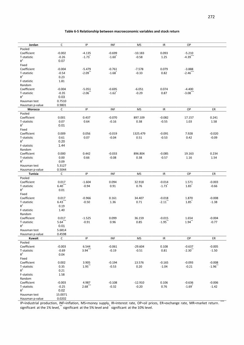
272
Table 6-5 Relationship between macroeconomic variables and stock return
Jordan C IP INF MS IR OP
Pooled
Coefficient -0.002 -4.135 -0.699 -10.183 0.093 -5.210
T-statistic -0.26 -1.73* -1.60* -0.58 1.25 -4.39***
R2 0.07
Fixed
Coefficient -0.004 -5.479 -0.761 -7.578 0.079 -3.888
T-statistic -0.54 -2.09** -1.68* -0.33 0.82 -2.46***
R2 0.23
F-statistic 1.81
Random
Coefficient -0.004 -5.051 -0.695 -6.051 0.074 -4.400
T-statistic -0.35 -2.06** -1.62* -0.29 0.87 -3.08***
R2 0.03
Hausman test 0.7510
Hausman p-value 0.9801
Morocco C IP INF MS IR OP ER
Pooled
Coefficient 0.001 0.437 -0.070 897.109 -0.082 17.157 0.241 T-statistic 0.07 0.64 -0.16 0.38 -0.55 1.03 1.58 R2 0.01
Fixed
Coefficient 0.009 0.056 -0.019 1325.479 -0.091 7.928 -0.020 T-statistic 0.61 0.07 -0.04 0.51 -0.53 0.42 -0.09 R2 0.20
F-statistic 1.44
Random
Coefficient 0.000 0.442 -0.033 896.804 -0.085 19.163 0.234 T-statistic 0.00 0.66 -0.08 0.38 -0.57 1.16 1.54 R2 0.09 Hausman test 5.3127 Hausman p-value 0.5044
Tunisia C IP INF MS IR OP ER
Pooled
Coefficient 0.017 -1.604 0.094 32.918 -0.014 1.571 -0.003 T-statistic 6.40*** -0.94 0.91 0.76 -1.73* 1.83* -0.66 R2 0.01
Fixed
Coefficient 0.017 -0.966 0.161 34.407 -0.018 1.870 -0.008 T-statistic 6.43*** -0.50 1.36 0.71 -2.11** 1.85* -1.38 R2 0.19
F-statistic 1.40
Random
Coefficient 0.017 -1.525 0.099 36.159 -0.015 1.654 -0.004 T-statistic 5.64*** -0.91 0.96 0.85 -1.95** 1.94** -0.77 R2 0.01
Hausman test 5.6814
Hausman p-value 0.4598
Kuwait C IP INF MS IR OP ER
Pooled
Coefficient -0.003 6.544 -0.061 -29.604 0.108 -0.637 -0.005 T-statistic -0.69 3.94*** -0.19 -0.51 0.81 -2.30** -1.50 R2 0.04
Fixed
Coefficient 0.002 3.905 -0.194 13.576 -0.165 -0.093 -0.008 T-statistic 0.35 1.95** -0.53 0.20 -1.04 -0.21 -1.96**
R2 0.21
F-statistic 1.58
Random
Coefficient -0.003 4.987 -0.108 -12.910 0.106 -0.636 -0.006 T-statistic -0.25 2.68*** -0.32 -0.20 0.76 -1.69* -1.42 R2 0.02
Hausman test 15.0071
Hausman p-value 0.0202
IP=industrial production, INF=inflation, MS=money supply, IR=interest rate, OP=oil prices, ER=exchange rate, MR=market return. ***
significant at the 1% level,
** significant
at the 5% level and
* significant
at the 10% level.

273
Table 6-6 Relationship between macroeconomic variables, market beta and stock returns
Jordan C IP INF MS IR OP MR
Pooled
Coefficient -0.0052 -3.6819 -0.7379 -14.4896 0.0839 -4.9189 0.0083
T-statistic -0.61 -1.47 -1.67* -0.77 1.11 -3.85*** 0.61
R2 0.07
Fixed
Coefficient -0.008 -4.431 -0.795 -13.934 0.080 -3.628 0.012
T-statistic -0.88 -1.49 -1.75* -0.56 0.83 -2.24*** 0.75
R2 0.24
F-statistic 1.80
Random
Coefficient -0.007 -4.360 -0.730 -11.858 0.075 -4.105 0.009
T-statistic -0.53 -1.61* -1.69* -0.52 0.87 -2.75*** 0.65
R2 0.03
Hausman test 1.1773
Hausman p-value 0.9780
Morocco C IP INF MS IR OP ER MR
Pooled Coefficient -0.012 0.194 -0.291 1,162.292 -0.105 17.069 0.247 0.021 T-statistic -0.71 0.27 -0.60 0.48 -0.69 1.02 1.62* 1.05 R2 0.01 Fixed Coefficient -0.009 -0.303 -0.404 1,872.284 -0.134 5.461 -0.022 0.032 T-statistic -0.48 -0.36 -0.76 0.72 -0.78 0.29 -0.10 1.47 R2 0.20 F-statistic 1.45 Random Coefficient -0.012 0.221 -0.239 1,132.995 -0.106 19.026 0.242 0.019 T-statistic -0.70 0.31 -0.50 0.48 -0.71 1.16 1.60* 0.98 R2 0.01 Hausman test 14.4780 Hausman p-value 0.0433
Tunisia C IP INF MS IR OP ER MR
Pooled Coefficient 0.022 -1.679 0.116 24.069 -0.014 1.252 -0.005 -0.007 T-statistic 3.54*** -0.98 1.09 0.54 -1.79* 1.33 -0.96 -0.83 R2 0.01 Fixed Coefficient 0.030 -0.963 0.242 6.215 -0.020 0.971 -0.013 -0.018 T-statistic 4.37*** -0.50 1.93** 0.12 -2.32** 0.88 -2.17** -2.02**
R2 0.20 F-statistic 1.41 Random Coefficient 0.022 -1.626 0.126 26.429 -0.016 1.310 -0.006 -0.007 T-statistic 3.59*** -0.97 1.18 0.60 -2.03** 1.41 -1.12 -0.95 R2 0.013 Hausman test 9.4157 Hausman p-value 0.2242
Kuwait C IP INF MS IR OP ER MR
Pooled Coefficient -0.006 6.574 -0.054 -33.048 0.106 -0.655 -0.005 0.003 T-statistic -0.34 3.93*** -0.17 -0.54 0.79 -2.19** -1.50 0.16 R2 0.04 Fixed Coefficient -0.013 4.061 -0.130 -4.654 -0.193 -0.120 -0.009 0.016 T-statistic -0.65 2.02** -0.35 -0.06 -1.19 -0.27 -2.02** 0.78 R2 0.20 F-statistic 1.56 Random Coefficient -0.006 6.574 -0.054 -33.048 0.106 -0.655 -0.005 0.003 T-statistic -0.34 3.93*** -0.17 -0.54 0.79 -2.19** -1.50 0.16 R2 0.043 Hausman test 15.2957 Hausman p-value 0.0324
IP=industrial production, INF=inflation, MS=money supply, IR=interest rate, OP=oil prices, ER=exchange rate, MR=market return. ***
significant at the 1% level,
** significant
at the 5% level and
* significant
at the 10% level
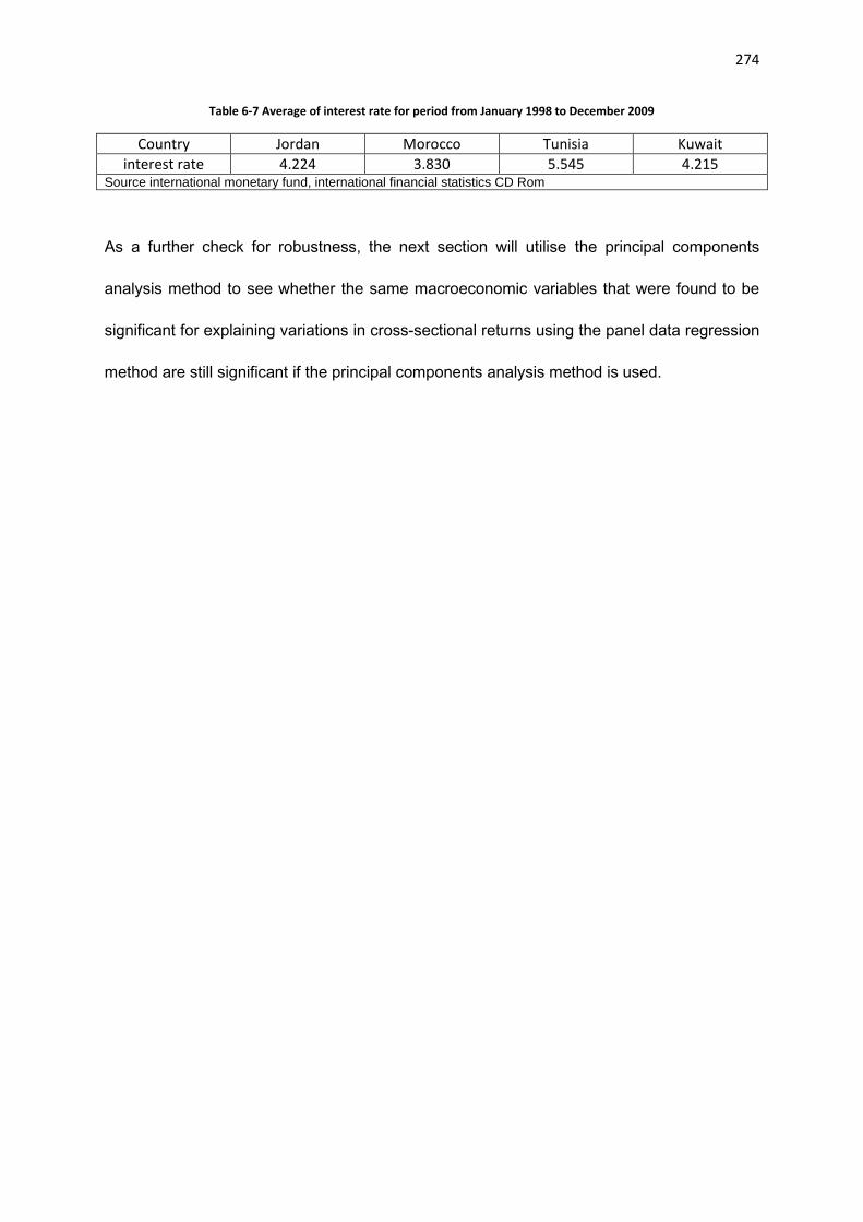
274
Table 6-7 Average of interest rate for period from January 1998 to December 2009
Country Jordan Morocco Tunisia Kuwait
interest rate 4.224 3.830 5.545 4.215 Source international monetary fund, international financial statistics CD Rom
As a further check for robustness, the next section will utilise the principal components
analysis method to see whether the same macroeconomic variables that were found to be
significant for explaining variations in cross-sectional returns using the panel data regression
method are still significant if the principal components analysis method is used.

275
6.4 Empirical results of testing relationship between
macroeconomic variables and stocks return using method of
principal components analysis.
This section will investigate the importance of macroeconomic variables in capturing the
variation of average stock returns for four Arab markets: Jordan, Morocco, Tunisia and
Kuwait using the method of principal components analysis (PCA). The advantage of using
PCA is to reduce six chosen macroeconomic variables to a much smaller set of K derived
orthogonal factors that retain the most information in six original macroeconomic variables.
The first step of using PCA is to determine correlation coefficients between macroeconomic
variables by using determinant value. However, the results reported in Table 6.8 show that
there is no relationship between macroeconomic variables, where the determinant value for
each market is greater than the critical value of 0.00001.
Table 6-8 Correlation coefficients between macroeconomic variables based on determinant value
The second step is factor extraction, which relies on eigenvalues associated with each
component. However, there are many principal components as macroeconomic variables.
In order to determine the number of principal components which retain the most information
in six original macroeconomic variables Kaiser criterion was used. According to this criterion
extracted principal components have eigenvalues greater than one. Tables 6.9 and 6.10
summarise the results of factor extraction for each market.
Country Jordan Morocco Tunisia Kuwait
determinant 0.696 0.849 0.833 0.655

276
Table 6-9 Extracted factors from six macroeconomic variables for four countries
Jordan
Initial Eigenvalues Extraction Sums of Squared Loadings Rotation Sums of Squared Loadings
Component Total
% of
Variance
Cumulative
% Total
% of
Variance
Cumulative
% Total
% of
Variance Cumulative %
1 1.420 28.391 28.391 1.420 28.391 28.391 1.390 27.790 27.790
2 1.128 22.557 50.949 1.128 22.557 50.949 1.158 23.159 50.949
3 0.984 19.676 70.624
4 0.828 16.559 87.184
5 0.641 12.816 100.000
Morocco
Initial Eigenvalues Extraction Sums of Squared Loadings Rotation Sums of Squared Loadings
Component Total
% of
Variance
Cumulative
% Total
% of
Variance
Cumulative
% Total
% of
Variance Cumulative %
1 1.146 19.093 19.093 1.146 19.093 19.093 1.134 18.904 18.904
2 1.109 18.486 37.579 1.109 18.486 37.579 1.106 18.440 37.344
3 1.054 17.560 55.139 1.054 17.560 55.139 1.068 17.794 55.139
4 0.953 15.881 71.019
5 0.904 15.074 86.093
6 0.834 13.907 100.000
Tunisia
Initial Eigenvalues Extraction Sums of Squared Loadings Rotation Sums of Squared Loadings
Component Total
% of
Variance
Cumulative
% Total
% of
Variance
Cumulative
% Total
% of
Variance Cumulative %
1 1.375 22.919 22.919 1.375 22.919 22.919 1.350 22.500 22.500
2 1.171 19.515 42.434 1.171 19.515 42.434 1.163 19.391 41.891
3 1.066 17.772 60.206 1.066 17.772 60.206 1.099 18.315 60.206
4 0.911 15.182 75.388
5 0.768 12.796 88.184
6 0.709 11.816 100.000
Kuwait
Initial Eigenvalues Extraction Sums of Squared Loadings Rotation Sums of Squared Loadings
Component Total
% of
Variance
Cumulative
% Total
% of
Variance
Cumulative
% Total
% of
Variance Cumulative %
1 1.382 23.026 23.026 1.382 23.026 23.026 1.376 22.926 22.926
2 1.297 21.617 44.642 1.297 21.617 44.642 1.303 21.716 44.642
3 0.981 16.342 60.985
4 0.899 14.982 75.967
5 0.790 13.160 89.127
6 0.652 10.873 100.000
All factors that have been selected their eigenvalues greater than 1

277
Table 6-10 Extracted factors from six macroeconomic variables and market return for four countries
Jordan
Initial Eigenvalues Extraction Sums of Squared Loadings Rotation Sums of Squared Loadings
Component Total
% of
Variance
Cumulative
% Total
% of
Variance
Cumulative
% Total
% of
Variance Cumulative %
1 1.617 26.957 26.957 1.617 26.957 26.957 1.612 26.865 26.865
2 1.169 19.491 46.447 1.169 19.491 46.447 1.175 19.583 46.447
3 0.986 16.428 62.875
4 0.944 15.742 78.617
5 0.770 12.829 91.446
6 0.513 8.554 100.000
Morocco
Initial Eigenvalues Extraction Sums of Squared Loadings Rotation Sums of Squared Loadings
Component Total
% of
Variance
Cumulative
% Total
% of
Variance
Cumulative
% Total
% of
Variance Cumulative %
1 1.346 19.232 19.232 1.346 19.232 19.232 1.212 17.315 17.315
2 1.129 16.131 35.362 1.129 16.131 35.362 1.186 16.939 34.254
3 1.060 15.142 50.504 1.060 15.142 50.504 1.118 15.964 50.219
4 1.046 14.943 65.448 1.046 14.943 65.448 1.066 15.229 65.448
5 0.926 13.226 78.674
6 0.861 12.299 90.973
7 0.632 9.027 100.000
Tunisia
Initial Eigenvalues Extraction Sums of Squared Loadings Rotation Sums of Squared Loadings
Component Total
% of
Variance
Cumulative
% Total
% of
Variance
Cumulative
% Total
% of
Variance Cumulative %
1 1.379 19.695 19.695 1.379 19.695 19.695 1.353 19.328 19.328
2 1.189 16.979 36.674 1.189 16.979 36.674 1.167 16.666 35.994
3 1.079 15.409 52.083 1.079 15.409 52.083 1.094 15.629 51.623
4 1.006 14.375 66.458 1.006 14.375 66.458 1.038 14.835 66.458
5 0.908 12.973 79.430
6 0.767 10.958 90.389
7 0.673 9.611 100.000
Kuwait
Initial Eigenvalues Extraction Sums of Squared Loadings Rotation Sums of Squared Loadings
Component Total
% of
Variance
Cumulative
% Total
% of
Variance
Cumulative
% Total
% of
Variance Cumulative %
1 1.696 24.235 24.235 1.696 24.235 24.235 1.654 23.626 23.626
2 1.304 18.623 42.858 1.304 18.623 42.858 1.192 17.029 40.655
3 1.013 14.472 57.330 1.013 14.472 57.330 1.167 16.675 57.330
4 0.926 13.230 70.560
5 0.809 11.556 82.116
6 0.668 9.549 91.665
7 0.583 8.335 100.000
All factors that have been selected their eigenvalues greater than 1
278
Table 6.9 shows the number of principal components extracted from six macroeconomic
variables for each market and also their latent roots. As can be seen from Table 6.9, the
number of principal components extracted differs for each market. A possible reason for this
is due to different degrees of response for each market to macroeconomic variables.
For Jordan the tables show there are two principal components that have latent roots greater
than one, the first component explains (28.391%) of total variance and the second
component explains (22.557%) of total variance and they are able to explain (50.949%) of
the total variance of original macroeconomic variables.
With regards to Morocco, three components are found to have latent roots greater than one,
they explain (19.232%), (18.486%) and (17.560%) of total variance respectively and all of
them explain (55.139%) of total variance of original macroeconomic variables.
Similar to Morocco Table 6.9 shows that three components are extracted for Tunisia, the first
component accounts for (22.919%) of variance, the second (19.515%) and the third
(17.772%) and together they explain (60.206%) of total variance.
Also Table 6.9 shows that two components are extracted for Kuwait, the proportion of
variance due to first and second components are (23.026%) and (21.617%) respectively,
and they are able to explain (44.642%) of total variance.
Table 6.10 shows the number of principal components extracted from six macroeconomic
variables in addition to market return for each market the reason why market return was

279
added to a set of macroeconomic variables is in a short period such as a single month
macroeconomic variables do not reflect all available information.
For Jordan Table 6.10 shows that the number of components is the same as Table 6.9,
which shows two components and their ability to explain total variance decrease from
(50.949 %) to (46.447%). A possible reason for the number of components being unchanged
for Jordan is due to excluding the exchange rate which is constant over the period from
January 1998 to December 2009. With regards to Morocco and Tunisia Table 6.10 shows
that the number of components increases from three components to four components and
also their ability to explain total variance increases from (55.139%), (60.206%) to (65.448%)
and (66.458%) respectively. For Kuwait, the results reported in Table 6.10 show the number
of components increases from two components to three components and they explain
(57.330%) of total variance.
Factors extracted from macroeconomic variables which account for the maximum amount of
variance are rotated in order to improve the interpretability of factors. Rotation maximises
the loadings of each macroeconomic variable on one of the extracted factors whilst
minimising the load on all other factors. These macroeconomic variables can then be used
to identify the meaning of the factor. The method used to rotate factors is orthogonal
rotation, which produces factors which are unrelated to or independent of one another.
An orthogonal rotation of principal components (factors) on six macroeconomic variables is
shown in Table 6.11, which displays macroeconomic variables load strongly on factors
(factor loadings greater than 0.50).

280
With regards to Jordan, Table 6.11 shows that money supply, inflation and oil prices which
represent costs load on the first factor, and industrial production which represents income
loads on the second factor. However, earlier tests of panel regression show that inflation and
oil prices were significantly negative, industrial production was significant but negative and
money supply was not found to be priced.
For Morocco, Table 6.11 shows that the first factor includes exchange rate and oil price
which represent international transaction. The second factor is correlated with inflation and
interest rate which represent costs, whereas the third factor is correlated with money supply
and industrial production which represent cash flows. Nevertheless, previous panel
regression showed that exchange rate only was found to be significant and positive.
In the case of Tunisia three factors are extracted. Exchange rate, inflation and money supply
which represent monetary policy load on the first factor and interest rate and oil price which
represent costs load on the second factor. Additionally, the results of panel regression
indicated that exchange rate and oil price are significant but oil price was positive. Industrial
production which represents income loads on the third factor.
For Kuwait the first factor is correlated with exchange rate, inflation and industrial production.
The second factor is correlated with money supply, interest rate and oil price which
represent cost. Previously, among six macroeconomic variables exchange rate, industrial
production and oil price were found significant.

281
In general, one can summarise that the first factor is correlated with exchange rate in three
countries: Morocco, Tunisia and Kuwait. Also it is correlated with inflation in three countries:
Jordan, Tunisia and Kuwait. Interest rate is loaded on the second factor in Morocco, Tunisia
and Kuwait. With regards to oil price it is correlated with the first factor in Jordan and
Morocco, and it is correlated with the second factor in Tunisia and Kuwait.
By adding market return to macroeconomic variables, the number and structure of factors
are changed as shown in Table 6.12. For Jordan the first factor includes market return,
money supply and oil price. With respect to Morocco, the number of factors increases to four
factors, the second factor (costs) is divided to two factors, the first is correlated with inflation
and market return, the second is correlated with interest rate. The first and third factors
become the second and fourth factors respectively. For Tunisia, Table 6.12 shows that the
number factors increase from three to four factors, the first three factors still the same, while
market return load on the fourth factor. The results in Table 6.12 for Kuwait indicate that the
number of factors increase to three factors. Market return, oil price and exchange are loaded
on the first factor. Interest rate and money supply are loaded on the second factor. Finally,
inflation is loaded on the third factor. Table 6.12 shows that the first factor includes market
return in three countries: Jordan, Morocco and Kuwait.
In order to test the relationship between factors extracted from macroeconomic variables
and return, the returns are regressed cross-sectionally against factors. The results of cross-
sectional regression are reported in Tables 6.13 and 6.14.
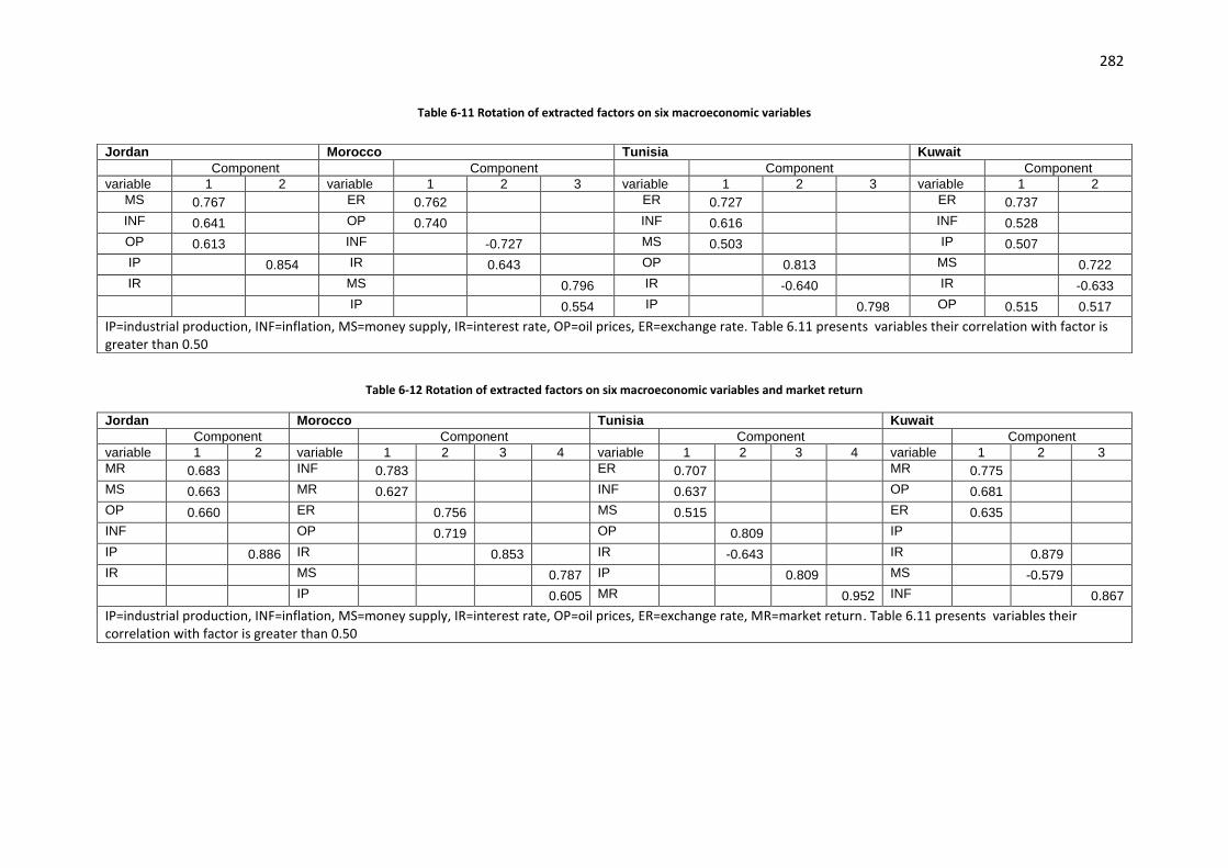
282
Table 6-11 Rotation of extracted factors on six macroeconomic variables
Table 6-12 Rotation of extracted factors on six macroeconomic variables and market return
Jordan Morocco Tunisia Kuwait
Component Component Component Component
variable 1 2 variable 1 2 3 4 variable 1 2 3 4 variable 1 2 3
MR 0.683 INF 0.783 ER 0.707 MR 0.775 MS 0.663 MR 0.627 INF 0.637 OP 0.681 OP 0.660 ER 0.756 MS 0.515 ER 0.635 INF OP 0.719 OP 0.809 IP IP 0.886 IR 0.853 IR -0.643 IR 0.879 IR MS 0.787 IP 0.809 MS -0.579 IP 0.605 MR 0.952 INF 0.867
IP=industrial production, INF=inflation, MS=money supply, IR=interest rate, OP=oil prices, ER=exchange rate, MR=market return. Table 6.11 presents variables their correlation with factor is greater than 0.50
Jordan Morocco Tunisia Kuwait
Component Component Component Component
variable 1 2 variable 1 2 3 variable 1 2 3 variable 1 2
MS 0.767 ER 0.762 ER 0.727 ER 0.737 INF 0.641 OP 0.740 INF 0.616 INF 0.528 OP 0.613 INF -0.727 MS 0.503 IP 0.507 IP 0.854 IR 0.643 OP 0.813 MS 0.722
IR MS 0.796 IR -0.640 IR -0.633
IP 0.554 IP 0.798 OP 0.515 0.517
IP=industrial production, INF=inflation, MS=money supply, IR=interest rate, OP=oil prices, ER=exchange rate. Table 6.11 presents variables their correlation with factor is greater than 0.50

283
Table 6.13 shows the results relationship between return and factors extracted from six
macroeconomic variables without market return. The results reported in Table 6.13 indicate
that the first factor is found to be statistically significant in Jordan at the 0.01 level and in
Kuwait at the 0.1 level, whereas it is not found to be significant in Morocco and Tunisia.
In addition Table 6.13 shows that the second factor is found to be significant in two
countries: Morocco and Kuwait at the 0.01 level. With respect to the third factor the results
reported in Table 6.13 provide evidence that is found to be significant in Morocco at the 0.05
level.
Clearly, the first factor for Jordan and Kuwait and the second factor for Morocco, which are
found to be significant, are correlated with inflation. In Jordan, Morocco and Kuwait a factor
correlated with money supply is found to be priced. Additionally, the second factor which is
found to be significant in Morocco and Kuwait is correlated with interest rate. The first and
third factors which are found to be significant in Kuwait and Morocco, respectively, contain
industrial production. Finally, the first factor and the second which are priced in Jordan and
Kuwait respectively are correlated with oil prices.
The most important differences between the results of panel data techniques reported in
Table 6.5 and PCA reported in Tables 6.13 are money supply, which is not found to be
significant using panel data is found important using PCA in Jordan, Morocco and Kuwait.
Using panel data techniques inflation is priced in Jordan, whilst using PCA the results show
that inflation is a significant variable in Jordan, Morocco and Kuwait.

284
For Morocco, the results of Table 6.5 show that there is no significant relationship between
return and any of the six macroeconomic variables. On the other hand, the results reported
in Table 6.13 reveal that the second factor includes inflation and interest rate and the third
factor includes money supply and industrial production are significant. In contrast to
Morocco, Table 6.5 shows that there is a significant relationship between return and interest
rate in Tunisia, while results reported in Table 6.13 for Tunisia reveal that there is no
relationship between stock returns and any extracted factor.
Table 6.14 shows the results of the cross-sectional regression between return and factors
extracted from six macroeconomic variables in addition to market return. The results reveal
that all factors correlated with market return are found to be statistically significant, with the
exception of Tunisia where all factors were found insignificant. Moreover, inflation for Jordan,
money supply and industrial production for Morocco and industrial production, money supply
and interest rate for Kuwait all which become uncorrelated with any factor when market
return was added to macroeconomic variables.
Table 6.14 shows that the first factor is statistically significant in three countries, Jordan,
Morocco and Kuwait, and in all countries the first factor correlated with market return. The
second factor is found to be priced in Morocco only. The third factor is found to be priced in
Morocco and Kuwait. Finally, Table 6.14 shows that there is no significant relationship
between return and the fourth factor in all countries.
As can be observed, the first factor for Jordan and Kuwait and the second factor for Morocco
which are found to be significant are correlated with oil price. The first and third factors which

285
are found to be significant in Morocco and Kuwait respectively contain inflation. Finally, the
first factor and the second which are priced in Kuwait and Morocco respectively are
correlated with exchange rate. Table 6.14 shows that R2 increased in Jordan, Morocco and
Kuwait with the inclusion market return to macroeconomic variables.
In summary, the results of panel data techniques and PCA reported in Tables 6.5, 6.6, 6.13
and 6.14 respectively indicate that oil price and inflation are important variables that have
influence on stock returns in Jordan. However, Table 6.14 shows that inflation becomes an
insignificant variable when market return was added to macroeconomic variables. With
regards to Kuwait, the results reported in Tables 6.5, 6.6, 6.13 and 6.14 reveal that the most
important variables are: oil price, exchange rate and industrial production. However, Table
6.14 shows that industrial production becomes an insignificant variable when market return
was added to macroeconomic variables. For Morocco and Tunisia the tables show that the
number of variables and their significance are different according to composition of
macroeconomic variables and the method used to estimate the relationship between stock
returns and macroeconomic variables.
Table 6-13 Cross-sectional regression of stock returns on factors are extracted from macroeconomic variables
Jordan Morocco Tunisia Kuwait
C 0.003 C 0.010 C 0.009 C 0.002
T-test 2.27** T-test 5.42*** T-test 7.60*** T-test 1.49
Factor1 0.186 Factor1 -0.037 Factor1 0.084 Factor1 0.140
T-test 2.61*** T-test -0.20 T-test 0.53 T-test 1.80*
Factor2 0.126 Factor2 -0.746 Factor2 0.013 Factor2 0.242
T-test 1.42 T-test -5.44*** T-test 0.11 T-test 2.89***
R2 0.18 Factor3 -0.333 Factor3 -0.085 R2 0.18
T-test -2.00** T-test -0.65
R2 0.73 R2 0.02 ***
significant at the 1% level,
** significant
at the 5% level and
* significant
at the 10% level. the results
reported in table 6.13 are obtained by regressing stocks returns cross-sectional against factors are extracted by using PCA

286
Table 6-14 Cross-sectional regression of stock returns on factors extracted from macroeconomic variables and market return
Using panel data regression for Morocco, Table 6.5 shows that there is not significant
macroeconomic variable that can explain variations in stock returns, but adding market
return to the set of macroeconomic variables, as in Table 6.6, shows that the exchange rate
becomes a significant variable. Using PCA, Tables 6.13 and 6.14 indicate that inflation and
interest rate are important variables that have an influence on stock returns in Morocco. With
regards to Tunisia, the results of panel data regression represented in Tables 6.5 and 6.6
show that the most important macroeconomic variable is interest rate. However, by adding
market return to set of macroeconomic variables, Table 6.6 shows that the macroeconomic
variables that are significant in explaining variations in stock returns are interest rate and
exchange rate. Comparing this with the results of panel data regression, the results of PCA
for Tunisia reported in Tables 6.13 and 6.14 show there are no macroeconomic variables
found to be significant.
Jordan Morocco Tunisia Kuwait
C 0.001 C 0.006 C 0.008 C -0.001
T-test 0.58 T-test 3.17*** T-test 3.41*** T-test -0.84
Factor1 0.191 Factor1 0.430 Factor1 0.104 Factor1 0.194
T-test 3.79*** T-test 4.99*** T-test 0.62 T-test 4.18***
Factor2 0.088 Factor2 -0.260 Factor2 0.013 Factor2 0.030
T-test 1.04 T-test -1.85* T-test 0.10 T-test 0.26
R2 0.25 Factor3 -0.218 Factor3 -0.089 Factor3 -0.162
T-test -1.85* T-test -0.67 T-test -1.63*
Factor4 -0.197 Factor4 0.026 R2 0.25
T-test -1.45 T-test 0.34
R2 0.83 R
2 0.02 ***
significant at the 1% level,
** significant
at the 5% level and
* significant
at the 10% level. the results
reported in table 6.14 are obtained by regressing stocks returns cross-sectional against factors are extracted by using PCA

287
6.5 Empirical results of testing relationship between market
liquidity and stocks return
Most previous empirical studies that tested the relationship between stock returns and
liquidity consider liquidity as a factor related to firm size, leverage, ratio of cash flow to stock
price, past sales growth, P/E ratio and book-to-market value, and they adopted Fama and
French’s three-factor model to examine the relationship between stock returns and liquidity,
among them the study of Datar et al (1998), Chan and Faff (2003), Martinez et al (2005) and
Marcelo and Quiros (2006).
Contrary to previous empirical studies which consider liquidity as factor related to firm, this
chapter considers liquidity as a factor related to the market and economy for reasons stated
in chapter three. According to that reasons turnover ratio which is computed as ratio of the
total value traded divided by market capitalisation will be used to measure aggregate market
liquidity. The explanation of using turnover ratio to measure market liquidity is the numerator
of this ratio total value traded depends on transaction costs, degree of trading and market
activity. The denominator of this ratio market capitalisation depends on the number of listed
firms and capital flows.
Because this study is focused on systematic risks, this chapter will use market liquidity
instead of asset liquidity. Additionally, this chapter will use CAPM and APT using pre-
specified macroeconomic approaches to test the relationship between market liquidity and
stock returns rather than the three-factor model of Fama and French (1992).

288
6.5.1 Empirical results of testing relationship between market liquidity
and stock returns using the CAPM
This sub-section will give the summary statistics for market liquidity, the relationship between
market liquidity and stock returns, and the relationship between market liquidity and stock
returns using CAPM as follows.
6.5.1.1 Summary statistics of market liquidity
Table 6.15 shows descriptive measures (summary statistics) which include mean, standard
deviation, maximum and minimum of market capitalisation, trading value and turnover ratio
of four markets.
Table 6-15 Summary statistics for market capitalisation, trading value and turnover ratio
As can be seen from Table 6.15 Kuwait has the highest market capitalisation which means
that Kuwait has the largest stock market, followed by Morocco and Jordan, while Tunisia has
Market capitalisation Trading value Turnover ratio
Jordan
Mean 37658.57 1544.393 0.039780
S.D 15722.70 948.0401 0.016520
Maximum 83881.00 4975.000 0.087863
Minimum 11203.00 221.0000 0.014376
Morocco
Mean 60140.46 1012.352 0.017646
S.D 23444.06 925.4310 0.012923
Maximum 93418.00 4369.000 0.060280
Minimum 14767.00 125.0000 0.003827
Tunisia
Mean 5476.501 79.95553 0.013692
S.D 1965.656 63.68671 0.008353
Maximum 9237.000 226.0000 0.036730
Minimum 2385.280 4.000000 0.000669
Kuwait
Mean 105931.7 10434.87 0.099594
S.D 27547.68 7558.513 0.081406
Maximum 147483.0 37477.00 0.544001
Minimum 52424.00 3452.530 0.036200

289
the lowest market capitalisation. Differences in market capitalisation among the four markets
is related to the number of listed companies in each market, for Kuwait and Jordan the
number of listed companies in December 2009 is (205) and (272) respectively, whereas for
Morocco and Tunisia the number is (73) and (52) respectively.
With regards to trading value Table 6.15 shows that Kuwait has the highest trading value
and Tunisia has the lowest. This refers to the Kuwaiti stock market being the most active
market and the Tunisian stock market being the less active market.
Tunisia has the lowest market capitalisation, trading value and smallest number of listed
companies, and this all leads to decreased market liquidity measured by turnover ratio. On
the other hand, increased market capitalisation, trading value and the number of listed
companies in the Kuwaiti stock market lead to increased market liquidity, despite Tunisian
stock market being more accessible to foreign investors than the Kuwaiti stock market. As a
result one can argue that the characteristics of the stock market have influences on market
liquidity.
6.5.1.2 The results of testing relationship between market liquidity and stock returns.
Regarding the relationship between stock returns and market liquidity and for the purpose of
comparison, Table 6.16 shows the results of regression between stock returns and market
liquidity, and Table 6.17 shows the results of regression between stock returns and market
liquidity using CAPM.

290
As can be observed from Table 6.16 there is a significant negative relationship between
stock returns and market liquidity in Jordan using pooled and random regressions and
negative and insignificant using fixed regression. With regards to Morocco Table 6.16 shows
that relationship stocks return and market liquidity is insignificant and positive using three
types of panel data regression. For Tunisia Table 6.16 indicates that the relationship
between stock returns and market liquidity is negative but insignificant. With regards to
Kuwait Table 6.16 shows that market liquidity plays a significant role in explaining stock
returns when pooled regression is used. However, using fixed and random regressions the
relationship between stocks returns and market liquidity is found to be negative but
insignificant.
As stated earlier, increased market capitalisation and trading value in the Kuwaiti and
Jordanian stock markets lead to increased role of market liquidity to explain variations in
average stock returns. Negative relationships between stock returns and market liquidity
found in Kuwait and Jordan is consistent with a study on Australian market by Chan and Faff
(2003), with studies on the US stock market by Datar et al (1998) and Gibson and Mougeot
(2004), and with a study on the Spanish stock market by Martinez et al (2005).
6.5.1.3 The results of testing relationship between market liquidity and stock returns
using CAPM.
The objective of using CAPM is to test whether the risk premium associated with the market
liquidity remains statistically negative and significant even in existence market beta. As can
be seen from the results reported in Table 6.17, there is no significant positive relationship
found between beta and stocks return in Jordan, Morocco and Kuwait using three types of

291
panel data regressions. These results are in agreement with what was found in chapter five
when four-moment CAPM was tested and in chapter six when the relationship between
stock returns and macroeconomic variable was examined. And it is also in line with the
results of studies of Datar et al (1998), Amihud (2002), Chan and Faff (2003) and Marcelo
and Quiros (2006) who found that beta has no ability to explain the cross-section variation in
stock returns.
For Tunisia the results reported in Table 6.17 show that the relationship between beta and
stock returns is a significant positive as postulated at 10% the level using pooled and
random regression. It is also noteworthy that beta is able to explain the cross-section
variation in stock returns in Tunisia when it is combined with market liquidity.
The results in Table 6.17 for market liquidity are similar to those reported in Table 6.16. The
results show that market liquidity remains able to explain the cross-section variation in stock
returns in Jordan at the 1% level using pooled and random regressions even if the market
beta is included in the analysis. In addition, the results for Jordan using fixed regression
show that the relationship between stock returns and market liquidity is negative as expected
but insignificant. For Jordan, these results imply that investors require less return on stocks
when the stock market is more liquid.
As shown in Table 6.17 there is no significant negative relationship between market liquidity
and stock returns in Morocco. The market liquidity remains unaffected even when market
beta is added to the regression model. As mentioned earlier, this is related to decreased
trading value and the number of listed companies. For Tunisia Table 6.17 shows that risk

292
Table 6-16 Relationship between market liquidity and stock returns
Table 6-17 Relationship between market liquidity and stock returns using CAPM
Jordan Morocco Tunisia Kuwait Variable Pooled Fixed Random Pooled Fixed Random Pooled Fixed Random Pooled Fixed Random
Y0 -0.003 -0.003 -0.003 0.013 0.01 0.01 0.015 0.015 0.015 -0.014 -0.013 -0.014 T-statistics -0.87 -076 -0.56 1.36
1.328
0.852
4.28
*** 4.41
*** 2.51
*** -2.29
** -2.44
*** -0.98
Y1 -0.018 -0.010 -0.017 0.004 0.00 0.01 -0.002 0.001 -0.001 -0.083 -0.024 -0.056 T-statistics -2.60
*** -0.89 -2.26
** 0.60 0.368 0.817 -0.51 0.22 -0.33 -1.94
** -0.53 -1.36
R2 0.02 0.30 0.02 0.00 0.30 0.00 0.00 0.30 0.00 0.01 0.43 0.01
F- statistics 1.13 1.24 1.28 2.11 Hausman Test 0.8407 0.0691 2.2136 2.6109
Hausman p-value 0.3592 0.7927 0.1368 0.1061 ***significant at 1% and **significant at 5%
Jordan Morocco Tunisia Kuwait Variable Pooled Fixed Random Pooled Fixed Random Pooled Fixed Random Pooled Fixed Random
Y0 -0.011 -0.011 -0.010 0.014 0.019 0.014 0.001 0.010 0.002 -0.023 -0.013 -0.020 T-statistics -0.98 -0.94 -0.94 0.65 0.795 0.56 0.12 0.99 0.16 -0.75 -0.43 -0.60 Y1 0.007 0.008 0.007 -0.001 -0.006 -0.001 0.015 0.006 0.014 0.009 -0.001 0.007 T-statistics 0.72 0.73 0.69 -0.03
-0.274 -0.07 1.64
* 0.59 1.61
* 0.29 -0.02 0.23
Y2 -0.018 -0.010 -0.018 0.004 0.312 0.007 -0.003 0.000 -0.003 -0.087 -0.024 -0.058 T-statistics -2.67
*** -0.88 -2.62
*** 0.59 0.004 0.81 -0.80 0.10 -0.73 -1.95
** -0.49 -1.34
R2 0.02 0.30 0.02 0.00 0.30 0.00 0.01 0.31 0.01 0.01 0.43 0.01
F- statistics 1.13
1.24 1.24 2.09 Hausman Test 0.8687 0.2556 8.9446 2.3122 Hausman p-value 0.6477 0.8800 0.0114 0.3147 *** Significant at 1%* Significant at 5%. ** Significant at 10%.

293
premium associated with the market liquidity is negative as expected using pooled random
regression but insignificant.
Finally, with regard to Kuwait Table 6.17 shows that market liquidity is only priced when fixed
affect regression model is used. This result is similar to those reported in Table 6.16
From the results shown in Tables 6.16 and 6.17 three general conclusions for Jordan and
Kuwait can be drawn. The first conclusion is there is a relationship between market activity
and market liquidity. The second conclusion is market liquidity remains able to explain the
cross-section variation in stock returns even if market beta is added to regression model.
The final conclusion is market beta was found to be priced in Tunisia only.
In order to see whether market liquidity is still an important variable to explain variation of
cross-sectional stock returns, the next section will test the relationship between stock returns
and market liquidity using APT pre-specified macroeconomic variables. As mentioned in
chapters one and three, the motivation behind testing market liquidity in the context of APT-
pre-specified macroeconomic variables is to find the interrelationship between market
liquidity and macroeconomic variables.

294
6.5.2 Empirical results of testing relationship between stocks return and
market liquidity using the APT pre-specified macroeconomic variables
This sub-section will show the empirical results of the relationship between stock returns and
market liquidity in the context of APT-pre-specified macroeconomic variables using panel
data regression and PCA as follows.
6.5.2.1 The results using panel data regression.
The relationship between stock return and liquidity has been very intensively investigated in
the market microstructure literature by adopting Fama and French’s three-factor model in
which the three factors are (i) the excess return on a broad market portfolio (ii) the difference
between the return on a portfolio of small stocks and the return on a portfolio of large stocks
and (iii) the difference between the return on a portfolio of high-book-to-market stocks and
the return on a portfolio of low-book-to-market stocks (Fama and French, 1996, pp55, 56).
However, empirical studies that test the relationship between stock returns and market
liquidity add market liquidity to three-factor model which is calculated as the difference
between the return on a portfolio of liquid stocks and the return on a portfolio of illiquid
stocks.
Contrary to previous empirical studies that measured liquidity as a variable related to
individual stocks and test its relationship with stock return within the context of the Fama and
French three-factor model, the current section will test the relationship between market
liquidity and stock returns by using aggregate market liquidity as a measure related to the
whole stock market, within the context of Chen et al’s (1986) APT pre-specified
macroeconomic variables model. This is motivated by the fact that liquidity relates to
characteristics of stock market, tightness, depth, and resiliency, which are influenced by

295
trading costs. Furthermore, aggregate market liquidity is largely determined by
macroeconomic variables that are systemic to the economy. If macroeconomic variables
anticipate economic recessions, they may also anticipate lower aggregate market liquidity
(Martinez et al, 2005).
By combining macroeconomic variables with market liquidity, Table 6.18 shows several
interesting observations. It shows that industrial production is found to be a significant
positive as expected in Morocco using fixed and random regressions and in Tunisia using
fixed regression when market liquidity is introduced. However, for Kuwait Table 7.4 shows
that the relationship between industrial production and stock return is positive but
insignificant. In the case of Jordan Table 6.18 shows that industrial production is found to be
an insignificant negative.
In terms of inflation, the results reported in Table 6.18 show that inflation is found to be
negative as postulated in Jordan, Morocco and Kuwait, but is not statistically significant.
Table 6.18 shows that the relationship between stock returns and inflation for Tunisia is a
significant positive.
Interest rate is found to be the most successful of independent variables which explain
average returns in Morocco and Tunisia, where it is found to be a significant negative by
using three types of panel data regressions. For Kuwait Table 6.18 shows that interest rate
is found to be negative but insignificant. In case of Jordan the results reported in Table 6.18
indicate that interest rate is not priced.

296
The relationship between money supply and stock returns is found to be a significant
negative as postulated in Jordan and Morocco and negative but insignificant in Kuwait,
whereas it is found to be positive and insignificant in Tunisia. The possible explanation for
negative relationship between money supply and stocks return is an increase in money
supply leads to increased inflation.
Regarding oil price, significant negative relationship at the 1% level is shown in Jordan using
three types of panel data regressions and in Kuwait at the 10% level using pooled and
random regressions. The relationship between exchange rate and stock returns is found to
be negative as postulated in Tunisia and Kuwait, but statistically insignificant, whereas for
Morocco it is positive and insignificant.
With regards to market liquidity Table 6.18 shows that four countries have a negative
relationship between stock returns and market liquidity, but statistically significant in Jordan
at the 1% level and in Tunisia at the 10% level.
However, Table 6.18 shows that there is no significant positive relationship between beta
and stock returns in Jordan, Morocco and Tunisia, and there is a significant positive
relationship between beta and stock return in Kuwait using fixed regression.
There are three interesting results that can be seen from Table 6.18: all countries have at
least two variables that are found to be important to explain the average of stock returns.
Variables are found to be priced differently across all countries. The risk premiums

297
associated with variables are found to be priced, and R2 are increased when fixed regression
is used.
By comparison with the results reported in Table 6.16, Table 6.18 shows that the relationship
between market liquidity and stock returns in existence of macroeconomic variables remains
a significant negative in Jordan and Tunisia. In addition, this relationship becomes
insignificant in Kuwait, and it is changed from negative to positive but statistically
insignificant in Morocco.
It can be seen that there are several conclusions regarding macroeconomic variables for
each country by comparing the results of Table 6.6 with the results of Table 6.18. The first is
the only variable consistently significant in explaining the cross-section of stock returns in
Jordan and Kuwait is oil price and in Tunisia is interest rate. The second is money supply
becomes a significant variable in Jordan and Morocco when market liquidity is added to
macroeconomic variables. The third is combination of market liquidity with macroeconomic
variables causes inflation and exchange rate to be insignificant across all countries. Finally,
by adding market liquidity to macroeconomic variables, industrial production and interest rate
become statistically significant in Morocco.
6.5.2.2 The results using PCA.
This sub-section tests the relationship between stock returns and market liquidity using the
APT pre-specified macroeconomic variables and PCA method in order to see whether
factors which include market liquidity is an important factor to explain cross-sectional returns.

298
Table 6-18 Relationship between market liquidity, macroeconomic variables, beta and stock returns
Jordan C IP INF IR MS OP ER ML MR Pooled Y 0.008 -2.276 -0.480 0.013 -74.288 -5.867 NA -0.022 0.016 T-test 0.51 -0.55 -0.81 0.12 -2.20
** -3.30
*** NA -2.37
*** 0.85
R2
0.14 Fixed Y 0.012 0.499 -0.728 0.167 -102.32 -8.242 NA -0.041 0.025 T-test 0.68 0.11 -1.20 1.22 -2.55
*** -3.67
*** NA -3.12
*** 1.22
R2
0.43 F-test 1.40 Random Y 0.007 -2.465 -0.515 0.011 -72.502 -5.938 NA -0.023 0.016 T-test 0.46 -0.61 -0.89 0.11 -2.15
** -3.39
*** NA -2.47
*** 0.82
R2
0.15 H-test 6.4930 P-value 0.4835
Morocco C IP INF IR MS OP ER ML MR Pooled Y 0.000 1.292 -0.454 -0.572 -5264 22.450 0.158 -0.003 0.013 T-test 0.02 1.11 -0.57 -1.83
* -1.94
** 1.24 0.71 -0.49 0.56
R2
0.05 Fixed Y 0.033 2.647 -0.705 -1.004 -8414 27.760 0.416 0.006 -0.029 T-test 1.70
* 2.05
** -0.79 -2.76
*** -3.03
*** 1.45 1.41 0.74 -1.02
R2
0.44 F-test 1.91 Random Y 0.008 1.787 -0.511 -0.707 -6321 26.260 0.273 -0.001 0.001 T-test 0.53 1.63
* -0.68 -2.36
*** -2.51
*** 1.55 1.30 -0.13 0.06
R2
0.06 H-test 25.0609 P-value 0.0015
Tunisia C IP INF IR MS OP ER ML MR Pooled Y 0.020 4.572 0.224 -0.015 14.747 -0.129 -0.004 -0.006 -0.008 T-test 2.65
*** 1.15 1.79
* -1.84
* 0.20 -0.10 -0.45 -1.62
* -0.72
R2
0.03 Fixed Y 0.024 8.385 0.346 -0.018 -3.661 -1.047 -0.013 -0.006 -0.019 T-test 2.86
*** 1.82
* 2.37
*** -2.07
** -0.04 -0.63 -1.19 -1.51 -1.43
R2
0.36 F-test 1.44 Random Y 0.020 5.436 0.225 -0.016 12.008 -0.424 -0.005 -0.006 -0.010 T-test 2.66
*** 1.37 1.83
* -2.00
** 0.16 -0.31 -0.57 -1.62
* -0.88
R2
0.03 H-test 4.2879 P-value 0.8303
Kuwait C IP INF IR MS OP ER ML MR Pooled Y -0.007 1.586 -0.457 -0.140 -54.575 -0.755 -0.003 0.025 0.014 T-test -0.25 0.50 -1.32 -1.07 -0.89 -1.87
* -0.64 0.79 0.52
R2
0.04 Fixed Y -0.045 -5.469 -0.374 -0.154 -37.356 -0.727 -0.006 -0.040 0.063 T-test -1.57 -1.01 -0.87 -0.96 -0.56 -1.43 -1.46 -1.07 1.92
**
R2
0.38 F-test 1.54 Random Y -0.007 1.697 -0.451 -0.140 -56.385 -0.763 -0.003 0.024 0.014 T-test -0.29 0.55 -1.33 -1.09 -0.94 -1.94
** -0.67 0.76 0.56
R2
0.04 H-test 23.2109 P-value 0.0031
IP=industrial production, INF=inflation, IR=interest rate, MS=money supply, OP=oil prices, ER=exchange rate, ML=market liquidity, MR= market return
*** significant
at the 1% level,
** significant
at the 5% level and
* significant
at the 10% level. NA
denotes unavailable because exchange rate for Jordan is constant for entire time period.

299
The results reported in Table 6.19 show that a determinant value for each market is greater
than the necessary value of 0.00001, which indicates that there is no relationship between
macroeconomic variables and market liquidity
Table 6-19 The correlation coefficients between macroeconomic variables and market liquidity based on determinant value
With regards to the number of principal components extracted from six macroeconomic
variables, market return and market liquidity which retain the most information in eight
original variables Table 6.20 shows that they are different across markets.
For Jordan Table 6.20 shows that there are three principal components that have latent
roots greater than one, the first component explains (23.792%) of total variance, the second
component explains (16.880%) of total variance and the third component explains (15.096%)
of total variance and together they are able to explain (55.768%) of total variance of original
variables.
With regards to Morocco Table 6.20 shows that there are four components that are found to
have latent roots greater than one, they explain (19.205%), (14.573%), (13.573%) and
(13.115%) of total variance respectively and all of them explain (60.467%) of total variance
of original variables.
As with Morocco Table 6.20 shows that four components are extracted for Tunisia, the
proportion of variance due to first, second, third and fourth components are (17.465%),
Country Jordan Morocco Tunisia Kuwait
determinant 0.668 0.761 0.812 0.618

300
(14.894%), (13.484%) and (13.037%) respectively, and their ability to explain total variance
is (58.880%).
For Kuwait, the results reported in Table 6.20 show that three components are extracted, the
first component accounts for (21.206%), the second (17.425%) and third (12.906%), and
together they explain (51.537%) of total variance.
Table 6.21 summarises the variable loadings for factors. For Jordan Table 6.21 shows that
the first factor had high correlations with inflation, money supply and oil prices, and this
principal component represents cost. The second factor is correlated with two market
variables: markets return and market liquidity. The third factor is correlated with industrial
production which represents the production sector and income.
In case of Morocco four factors are extracted. Inflation and market return load on the first
factor. Money supply and market liquidity which represent cash flows load on the second
factor. The third factor is correlated with exchange rate and oil prices and this factor
represents international transactions. The fourth factor had a high loading on interest rates.
As with Morocco, in Tunisia four factors are extracted. Three variables, exchange rate,
inflation and money supply, are correlated with the first factor which represents monetary
policy. The second factor represents cost and is correlated with interest rates and oil prices.
The third factor is correlated with industrial production which represents the production
sector and income. The fourth factor is correlated with two market variables: markets return
and market liquidity.

301
Table 6-20 Extracted factors from six macroeconomic variables and market liquidity for four countries
As can be seen from Table 6.21, inflation is correlated with the first factor in Jordan,
Morocco and Tunisia, industrial production is correlated with the third factor in Jordan and
Jordan
Initial Eigenvalues Extraction Sums of Squared Loadings Rotation Sums of Squared Loadings
Component Total % of
Variance Cumulative
% Total % of
Variance Cumulative
% Total % of
Variance Cumulative %
1 1.665 23.792 23.792 1.665 23.792 23.792 1.483 21.189 21.189 2 1.182 16.880 40.672 1.182 16.880 40.672 1.264 18.056 39.244 3 1.057 15.096 55.768 1.057 15.096 55.768 1.157 16.524 55.768 4 0.978 13.966 69.735 5 0.849 12.126 81.861 6 0.762 10.880 92.741 7 0.508 7.259 100.000
Morocco
Initial Eigenvalues Extraction Sums of Squared Loadings Rotation Sums of Squared Loadings
Component Total % of
Variance Cumulative
% Total % of
Variance Cumulative
% Total % of
Variance Cumulative %
1 1.536 19.205 19.205 1.536 19.205 19.205 1.240 15.494 15.494 2 1.166 14.573 33.778 1.166 14.573 33.778 1.220 15.254 30.749 3 1.086 13.573 47.351 1.086 13.573 47.351 1.220 15.247 45.996 4 1.049 13.115 60.467 1.049 13.115 60.467 1.158 14.471 60.467 5 0.926 11.574 72.041 6 0.874 10.923 82.964 7 0.740 9.250 92.214 8 0.623 7.786 100.000
Tunisia
Initial Eigenvalues Extraction Sums of Squared Loadings Rotation Sums of Squared Loadings
Component Total % of
Variance Cumulative
% Total % of
Variance Cumulative
% Total % of
Variance Cumulative %
1 1.397 17.465 17.465 1.397 17.465 17.465 1.384 17.301 17.301 2 1.192 14.894 32.360 1.192 14.894 32.360 1.177 14.714 32.015 3 1.079 13.484 45.843 1.079 13.484 45.843 1.080 13.504 45.519 4 1.043 13.037 58.880 1.043 13.037 58.880 1.069 13.361 58.880 5 0.984 12.303 71.184 6 0.906 11.322 82.506 7 0.756 9.445 91.950 8 0.644 8.050 100.000
Kuwait
Initial Eigenvalues Extraction Sums of Squared Loadings Rotation Sums of Squared Loadings
Component Total % of
Variance Cumulative
% Total % of
Variance Cumulative
% Total % of
Variance Cumulative %
1 1.696 21.206 21.206 1.696 21.206 21.206 1.670 20.872 20.872 2 1.394 17.425 38.631 1.394 17.425 38.631 1.290 16.125 36.997 3 1.032 12.906 51.537 1.032 12.906 51.537 1.163 14.540 51.537 4 0.971 12.134 63.671 5 0.926 11.576 75.247 6 0.768 9.604 84.851 7 0.629 7.857 92.708 8 0.583 7.292 100.000
All factors that have been selected their eigenvalues greater than 1

302
Tunisia. Finally, market return and market liquidity is load on the second factor in Jordan and
the fourth factor in Tunisia.
In order to investigate the relationship between factors extracted from macroeconomic
variables and market liquidity which are reported in Tables 6.20 and 6.21, and return, the
final step of the analysis uses these factors as inputs to a regression analysis.
Table 6.22 shows the results of cross-sectional regression of stocks returns on factors are
extracted from macroeconomic variables and market liquidity. The results reported in Table
6.22 show that one factor is found to be statistically significant in each country with the
exception of Tunisia where the results show there is not any significant factor.
The factor found to be statistically significant is the first factor in Morocco and Kuwait and the
second factor in Jordan. For Jordan the second factor is correlated with market return and
market liquidity. In Morocco the first factor is correlated with inflation and market return. For
Kuwait the first factor contains three macroeconomic variable: exchange rates, oil prices and
market return.
It is noteworthy that the common variable among factors that have been found significant in
Jordan, Morocco and Kuwait is market return. Furthermore, the variables that remain
significant in explaining cross-sectional returns are market liquidity for Jordan and oil prices
for Kuwait.

303
Table 6-21 Rotation of extracted factors on six macroeconomic variables and market liquidity
Table 6.21 reports the results of rotation of extracted factors on six macroeconomic and market liquidity Jordan Morocco Tunisia Kuwait
Component Component Component Component
variable 1 2 3 variable 1 2 3 4 variable 1 2 3 4 variable 1 2 3
INF 0.615 ER 0.769 ER 0.678 ER 0.648 IP 0.852 INF 0.755 INF 0.598 INF 0.571 IR IP IP 0.768 IP MS 0.703 IR 0.829 IR -0.698 IR 0.907
OP 0.664 MS 0.717 MS 0.641 MS -0.549 MR 0.664 OP 0.680 OP 0.775 OP 0.657 MLQ -0.762 MR 0.630 MR 0.715 MR 0.772 MLQ 0.587 MQ 0.732 MLQ 0.675 IP=industrial production, INF=inflation, MS=money supply, IR=interest rate, OP=oil prices, ER=exchange rate, MR=market return and MLQ= market liquidity. Table 6.21 presents variables their correlation with factor is greater than 0.50

304
Table 6-22 Cross-sectional regression of stock returns on factors extracted from macroeconomic variables and market liquidity
Jordan Morocco Tunisia Kuwait
C 0.001 C
0.005 C 0.008 C
-0.001
T-test 0.35 T-test 2.95***
T-test 3.08***
T-test -0.49
Factor1 0.118 Factor1
0.431 Factor1
0.140 Factor1 0.199
T-test 1.43 T-test 4.86
*** T-test 0.87 T-test 4.05
***
Factor2 0.153 Factor2
-0.125 Factor2 -0.003 Factor2
-0.026
T-test 1.73*
T-test -0.77 T-test -0.03 T-test -0.28
Factor3 0.120 Factor3
-0.220 Factor3 -0.058 Factor3
-0.051
T-test 1.34 T-test -1.50 T-test -0.46 T-test -0.41
R2
0.25 Factor4 -0.184 Factor4
0.065 R2 0.22
T-test -1.60 T-test 0.62
R2 0.82 R
2 0.034
*** significant
at the 1% level and
* significant
at the 10% level. the results reported in table 6.22 are
obtained by regressing stocks returns cross-sectional against factors are extracted by using PCA

305
6.6 Summary
The main objective of this chapter was to investigate whether macroeconomic variables:
industrial production, inflation, money supply, interest rate, oil price, exchange rate, in
addition to , market liquidity and stock returns are able to explain variations in stock returns
in four Arabic countries; Jordan, Morocco, Tunisia and Kuwait, during the period January
1998 to December 2009. This objective is realised through three questions; the first is to
what extent can macroeconomic variables using APT explain variations in Arab stock
market? The second is to what extent can aggregate market liquidity explain variations in
Arab stock market? The third is do beta, macroeconomic variables and aggregate market
liquidity remain significant variables for explaining variations in Arab stock market when they
are combined in one model? The first question was motivated by the lack of economic
meaning attached to the factors obtained from factor analyses run by previous studies, and
practical evidence indicating that firms use macroeconomic variables as additional risk
factors when they calculate the cost of capital and evaluate a project. The second question
was motivated by four facts: within markets there is a transaction cost that has an influence
on the value traded and hence market liquidity; furthermore market liquidity is related to
characteristics of a stock market, including its size, regulation and supervision; there is a
relationship between market liquidity and macroeconomic variables; and a liquid stock
market enables investors to modify their portfolios quickly and cheaply.
To accomplish the objective of this chapter, APT was used together with two techniques to
test it: panel data and PCA. A modified method of Fama and MacBeth (1973) was adopted
to utilise panel data technique. According to this method three steps were used to test the
relationship between macroeconomic variables and stocks return. The first step was portfolio

306
formation, in this step which covered the period from extending from January 1998 to
December 2000, individual stocks were grouped into portfolios according to their beta,
skewness and then kurtosis. In the second step, which covered the period of 36 months from
January 2001 to December 2003, time-series regression was used to estimate betas of
macroeconomic variables by regressing portfolio return, which was constructed in the first
step against macroeconomic variables. The third step was the testing period. In this step,
which covered the time period from January 2004 to December 2009, the returns of all
portfolios over the sample period were regressed against betas of the macroeconomic
variables which were computed in the second step, to test the relationship between the
macroeconomic variables on one hand and market liquidity and stock returns on the other. In
the third step of panel data regression two combinations of macroeconomic variables were
tested, the first macroeconomic variables without market return and the second
macroeconomic variables with market return.
The empirical results of the first combination revealed that industrial production was
significantly positive in Kuwait, while insignificantly negative in others countries. This result
implies stock prices in Kuwait respond to future cash flow. With regards to inflation the
results showed that it was significantly negative in Jordan and insignificantly negative in
Morocco and Kuwait, and an insignificant positive in Tunisia. For Jordan this result confirms
the postulated hypotheses that increased inflation leads to increased discount rate and
hence decreases stock price. As regards interest rate, the results indicated that it was found
to be a significant negative as expected in Tunisia. As discussed in section 6.3 the
significant effect of interest rate can be explained by increases in the average of interest rate
in Tunisia than others countries. This means increased cost of borrowing and decreased

307
profits and stock prices. The relationship between stock returns and oil price was found to be
significantly negative, as postulated for Jordan and Kuwait, even though Jordan is a net oil
importer and Kuwait is a net oil exporter.
However, the results showed that there was no significant relationship between stock returns
and money supply in all countries, which indicated that the monetary policy of central banks
in these countries did not have any impact on their stock markets. Furthermore, the
exchange rate was found to be significantly negative in Tunisia and Kuwait using fixed effect
regression. This significant negative relationship between exchange rates and stock returns
in Tunisia and Kuwait reflects a policy of the depreciation of the national currency against
foreign currencies in order to increase exports, profits and stock returns. For Morocco the
exchange rate is found to be a significant positive as expected. One explanation for this
phenomenon is appreciation of national currency against foreign currency leads to increases
in consumption, particularly capital goods (growth investment opportunities), profits and
stock returns.
The empirical results of the second combination revealed that the only variables consistently
significant in explaining variations in cross-sectional return were inflation and oil price for
Jordan, interest rate for Tunisia and industrial production, oil price and exchange rate for
Kuwait and when market return was added to the set of macroeconomic variables it was
found to be not priced, which indicates that investors were not compensated for market risk.
As a further check for results of panel data regressions the PCA method was employed to
test the relationship between stock returns and macroeconomic variables. Moreover, the

308
justification behind using this method was PCA that combines two or more than two
variables into one factor, and while a variable may appear to be unimportant by itself it may
assume a more prominent role when evaluated jointly with other variables. Using the PCA
method two combinations of macroeconomic variables were tested. The first macroeconomic
variables were without market return and the second macroeconomic variables were with
market return.
The empirical results of the first combination indicated that the number of significant factors
vary across countries. For Jordan the first factor was found to be significant. In the case of
Morocco the second and third factors were found to be significant. For Kuwait the first and
second factors were found to be significant. There was no significant relationship between
stock returns and any factors in Tunisia. Common macroeconomic variables among those
significant factors in three or two countries are: money supply, inflation, oil price, interest rate
and industrial production.
The empirical results of the second combination by adding market return to macroeconomic
variables indicated that the number of significant factors for Morocco changes from two to
three factors, while for Jordan, Tunisia and Kuwait it does not change. Common
macroeconomic variables among those significant factors are: market return, oil price,
inflation and exchange rate. The advantage of using PCA was that money supply and
market return became important variables whereas they were unimportant variables when
panel data was used.

309
In summary, the results of panel data regression and PCA using two combinations of
macroeconomic variables without and with market return revealed that the most important
variables that remain significant for Jordan is oil price and for Kuwait are oil price and
exchange rate.
To achieve the objective related to the second question, which tested the relationship
between market liquidity and stock returns, turnover ratio (which is computed as ratio of the
total value traded divided by market capitalisation) was used to measure aggregate market
liquidity. In addition to the CAPM and APT pre-specified macroeconomic approach panel
data and PCA method were used to test the relationship between market liquidity and stock
returns.
Testing the relationship between stock returns and market liquidity alone the empirical
results show there is a significant negative relationship between stock returns and market
liquidity, as expected in Jordan using pooled and random regressions and in Kuwait using
pooled regression. While in Morocco and Tunisia the results show there is no significant
negative relationship between stock returns and market liquidity because they are thinly
traded markets compared with the Jordan and Kuwait stock markets.
.
Using CAPM the results show that beta was found to be significant positive only in Tunisia,
and the relationship between stock returns and market liquidity was unchanged in four
countries. Therefore, the results show that market liquidity plays an important role in more
active and liquid market (Jordan and Kuwait) which is measured by trading value and
turnover ratio than inactive illiquid market (Morocco and Tunisia).

310
The second approach used to test the importance of market liquidity to explain stock returns
is APT using pre-specified macroeconomic approach. The results of panel indicated that
there are three important independent variables to explain stocks return in Jordan, Morocco
and Tunisia; these variables for Jordan are money supply, oil price and market liquidity, for
Morocco are industrial production, interest rate and money supply and for Tunisia are
industrial production, interest rate and market liquidity. With regards to Kuwait two
independent variables were found to be important to explain stocks return, these variables
are oil price market return.
With respect to Jordan, money supply and market liquidity were found to be significant
variables which reflected influence of liquidity of the central bank and stock market on stock
prices. Industrial production, interest rate and money supply were found to be significant
variables in Morocco indicating the influence of economic growth and monetary policy on
stock prices. Regarding Tunisia, three variables were found to be significant: industrial
production, interest rate and market liquidity; implying that economic growth, monetary policy
and market liquidity explain variations in stock returns. For Kuwait the importance of oil price
and market return indicated that the cost of fuel had influence on stock price and investors
were compensated for market risk.
It is worth noting that oil price is a common variable in Jordan which is a net oil importer and
Kuwait which is a net oil exporter, whereas interest rate is a common variable in Morocco
which has the lowest interest rate and Tunisia which has the highest interest rate. However,
industrial production and market liquidity for Tunisia and beta for Kuwait were found to be

311
significant when macroeconomic variables, market liquidity and beta were included in one
regression model.
The results of PCA method indicated that one factor is found to be significant in Jordan,
Morocco and Kuwait and variables that remain significant in explaining cross-sectional
returns are market liquidity for Jordan and oil prices and market return for Kuwait.
Generally, this chapter reveals that some macroeconomic variables are important in
explaining stock returns and their significance varies across countries, which may be related
to specific characteristics of the economy of each country. Additionally this chapter reveals
that market liquidity appears to have the most consistent significant effect on active and
large stock markets.

312
Chapter 7 Conclusion
7.1 Introduction.
This study empirically examined conditional four-moment CAPM and APT pre-specified
macroeconomic variables with market liquidity in Arab stock markets, namely: the Amman
Stock Exchange, the Casablanca Stock Exchange, the Tunisian stock Exchange and the
Kuwait Stock Exchange.
The examination of conditional four-moment CAPM and APT pre-specified macroeconomic
variables with market liquidity in this study was based on four questions; the first was to
what extent can unconditional and conditional four-moment CAPM explain variations in Arab
stock markets? The second, to what extent can macroeconomic variables using APT explain
variations in Arab stock markets? Thirdly, to what extent can aggregate market liquidity
explain variations in Arab stock markets? Fourthly, do beta, macroeconomic variables and
aggregate market liquidity remain significant factors for explaining variations in Arab stock
markets when they are combined in one model?
The motivations behind testing four-moment CAPM and APT pre-specified macroeconomic
variables with market liquidity, based on the four questions above were: there is wide
acceptance in financial literature and practice that CAPM is the most common method used
to estimate the cost of capital and evaluate the performance of managed funds; empirical
evidence confirms that emerging market returns are not normally distributed; and there is
skewness and kurtosis in emerging markets. Using a conditional approach to test four-
moment CAPM was motivated by the fact that there were no expected returns which exceed

313
the risk-free return for stocks and the market, as CAPM assumes. There is also a lack of
economic meaning attached to the factors obtained from factor analysis to test APT, and
practical evidence indicating that firms use macroeconomic variables as additional risk
factors, when they calculate the cost of capital and evaluate a project. There is a transaction
cost which has an influence on value traded and hence market liquidity, market liquidity is
related to characteristics of stock market, size, regulation and supervision, there is also a
relationship between market liquidity and macroeconomic variables, and a liquid stock
market enables investors to modify their portfolios quickly and cheaply.
The investigation of four-moment CAPM and APT pre-specified macroeconomic variables
with market liquidity used a sample of 194 stocks, 48 for the Amman Stock Exchange, 32 for
the Casablanca Exchange, 32 for the Tunisia Stock Exchange and 82 for the Kuwait Stock
Exchange, during a period from January 1998 to December 2009.
The following sections present the conclusion of the investigation into four-moment CAPM
and APT pre-specified macroeconomic variables with market liquidity in terms of theory,
methodology and empirical results.
7.2 Conclusion of conditional four-moment CAPM.
Chapter two theoretically reviews empirical studies of conditional four-moment CAPM. The
four-moment CAPM was developed from two- and three-moment CAPM. Two-moment
CAPM builds on Markowitz’s model of mean–variance and it assumes there is an
unconditional positive relationship between beta and stock return, asset returns are normally
distributed and three- and four-moment (skewness and kurtosis) would be expected to have

314
mean values of zero. Since asset returns do not follow normal distribution, investors prefer
stock with high-positive skewness and low kurtosis. Kraus and Litzenberg (1976) developed
three-moment CAPM by incorporating co-skewness to two-moment CAPM. Three-moment
CAPM assumes an unconditional positive relationship between beta and stock return and an
unconditional relationship between co-skewness and stock return, which is opposite to
market skewness. Fang and Lai (1997) developed three-moment CAPM to four-moment
CAPM by adding co-kurtosis. Four-moment CAPM assumes an unconditional positive
relationship between beta and co-kurtosis and stock return, and an unconditional
relationship between co-skewness and stock return which is opposite to market skewness.
Two-moment CAPM is based on the assumption that expected return is always more than
risk-free return and that therefore there is an unconditional positive relationship between
beta and stock return. Given that there is no expected data for market portfolio return and
stock returns in the real world, empirical tests of two-moment CAPM utilise realised return on
market portfolio and stocks which may be less than the risk-free return, instead of the
expected return on market portfolio and stocks, to test two-moment CAPM and they found a
negative relationship between beta and return. To find a positive relationship between beta
and return by using realised return on market portfolio and stocks, Pettengill et al (1995)
developed conditional two-moment CAPM that relies on separation between periods which
have positive realised return (realised return is more than risk-free return), and periods which
have negative realised return (realised return is less than risk-free return). According to
conditional two-moment CAPM there will be a positive relationship between beta and return
in periods when realised return is more than risk-free return (up market), and a negative

315
relationship between beta and return in periods when realised return is less than the risk-free
return (down market).
Methodologically, chapter four showed that panel data regressions were used to test
unconditional and conditional four-moment CAPM in this study, whereas previous studies
employed cross-section regression to test four-moment CAPM. The main motivation behind
using panel data regressions was the small size of sample for each stock market included in
this study. Among the advantages of panel data are: the sample size can be increased
considerably by using a panel data and hence much better estimates can be obtained; also
by using panel data, one can increase the number of degrees of freedom, and thus the
power of the test.
Chapter five provides the empirical results of testing the first question, which examines the
ability of unconditional and conditional four-moment CAPM to explain variations in stock
returns. The results of unconditional four-moment CAPM showed that beta was not found to
be priced in Morocco, Tunisia and Kuwait using either EWI or VWI, which implies that
investors do not compensate for market risk, market portfolio is not efficient and variables
other than beta may explain the relationship between risk and return. These results were in
agreement with the findings of Chan et al (1991), Wong and Tan (1991), Fama and French
(1992, 1996, 2004), Fletcher (1997, 2000), Strong and Xu (1997), Datar et al (1998),
Hodoshima et al (2000), Amihud (2002), Chan and Faff (2003), Ho et al (2006), Morelli
(2007), Lam and Li (2008) and Fu (2009) who found that beta was not priced. Beta was
found to be priced in Jordan using VWI only. Unsystematic risk was used to test whether
investors held the market portfolio, and whether the market portfolio was efficient as

316
assumed by CAPM. The test was an attempt to judge the idea that CAPM is a inadequate to
explain variation in stock return, and measurements other than beta explain variations in
cross sectional returns. The results showed no significant positive relationship between
unsystematic risk and stock returns. These results led to the rejection of the idea that
investors are compensated for bearing unsystematic risk and indicated that CAPM was not a
inadequate to explain variation in stock return. These results were parallel to the results of
Hawawini et al (1983), Wong and Tan (1991), Cheung and Wong (1992) and Cheung et al
(1993), who found no significant positive relationship between unsystematic risk and stock
returns. With regards to co-skewness, the results demonstrated that it was found to be
priced in Morocco and Jordan using EWI and VWI respectively, which implies that investors
prefer positive co-skewness and forego the expected return for taking the benefit of
increasing the co-skewness. These results are in accordance with the results of Kraus and
Litzenberger (1976) and Lim (1989) who found that the co-skewness was priced. As with
unsystematic risk, the results for the four stock markets showed there was no significant
positive relationship between co-kurtosis and stock returns, which implies that investors are
not compensated by higher expected return for bearing co-kurtosis. The finding that co-
kurtosis is not priced is opposite to evidence provided by Fang and Lai (1997), David and
Chaudhry (2001), Liow and Chan (2005) and Doan et al (2010) who found that co-kurtosis
was priced and that it is important in explaining stock returns.
As a further investigation, unconditional four-moment CAPM was modified to conditional
four-moment CAPM based upon whether a market was up or down. Taking that modification
into account, there were two kinds of relationship between beta, co-skewness and co-

317
kurtosis and stock returns, one when a market was up and another when a market was
down.
The empirical results of univariate regression for all countries indicate that there existed a
strong positive (negative) relationship between beta and return in up (and down) markets
using EWI and VWI as proxies for market portfolio, despite market return on average being a
negative in Morocco, Tunisia and Kuwait. These results were consistent with the findings of
many previous studies, among them Pettengill et al (1995, 2002), Fletcher (1997, 2000),
Hodoshima et al (2000), Ho et al (2006) and Morelli (2007, 2011). The results of multivariate
regression that contained one dependent variable, return, and two independent variables,
beta and unsystematic risk, showed that beta remained significant in Jordan, Morocco and
Kuwait, even when unsystematic risk was introduced. Beta only loses its explanatory power
in the case of Tunisia in up and down markets using EWI. Unsystematic risk was found to be
a significant positive (negative) in up (and down) markets, except for Morocco using EWI
and when market was down, and for Morocco and Tunisia using VWI and when market was
up; this means that investors in these countries did not hold a diversified portfolio. If so,
unsystematic risk would have been insignificant in both up and down markets.
The empirical results of three-moment CAPM revealed that there was a statistically
significant relationship between co-skewness and stock returns, and that co-skewness had a
sign opposite to market skewness in Jordan and Tunisia, in both up and down markets and
utilising both EWI and VWI. These results are similar to the findings of Galagedera et al
(2003) and Tang and Shum (2006) who found that the relationship between co-skewness
and return is negative (positive) in up (and down) markets. Using EWI in an up market, co-

318
skewness in Morocco had the sign three-moment CAPM assumes, but was insignificant.
However, in Kuwait co-skewness had the same sign as market skewness, which is
considered contrary to the prediction of three-moment CAPM. Co-skewness in Morocco was
found be positive (negative) in up (and down) markets when VWI was employed, which was
not in agreement with the assumptions of the theory of three moment CAPM.
The empirical results of four-moment CAPM utilising EWI and VWI reveal that beta remains
a significant positive (negative) in up (and down) market in all stock markets, even when co-
skewness and co-kurtosis were introduced. Using EWI, co-skewness was found to be
significant in Jordan when the market was up and significant in all stock markets when the
market was down. Co-kurtosis was found to be insignificant across all stock markets when
the market was up. Contrary to up market, in down market co-kurtosis was significant in
Tunisia and Kuwait.
Employing VWI, the results of four-moment CAPM show that in Tunisia the relationship
between co-skewness and return is negative (positive) in up (and down) market. In addition,
the relationship between co-kurtosis and return was positive (negative) in up (and down)
markets. These results are considered considerable support for the prediction of four-
moment CAPM.
For Jordan, the co-skewness was found to be statistically significant and remained
statistically significant even after introducing co-kurtosis in up and down markets, using both
EWI and VWI. A similar situation was found in Tunisia.

319
The outperformance of conditional two-, three- and four-moment CAPM is attributed to using
realised returns (ex-post), which might be more or less than accurate expectations, and the
relationship between beta, co-skewness and co-kurtosis and return were different when
realised returns were more than accurate expectations (up market) and when realised
returns were less than accurate expectations (down market).
The main practical contribution of testing unconditional and conditional four-moment CAPM
is the application of panel data regressions (pooled, fixed and random regression) where
previous studies have used the cross-section method to test four-moment CAPM. The
advantages of using panel data regressions were: the sample size was increased; much
better estimates were obtained; there was an increase the number of degrees of freedom;
there was therefore an increase in the power of the test. In addition, the advantage of using
panel data regressions is that there was positive (negative) relationship between beta and
return in up (and down) markets for all countries, statistically significant negative (positive)
relationship between co-skewness and stock returns in up (down) markets, and co-
skewness had a sign opposite to market skewness in Jordan and Tunisia and a statistically
significant positive (negative) relationship between co-kurtosis and return in up (and down)
markets in Tunisia. Market return on average was a negative in Morocco, Tunisia and
Kuwait, which is considered opposite to the first condition for testing conditional CAPM,
which states that market excess return on average should be positive. Additionally, the
number of down market months was more than up market months.
The main findings of chapter five can be classified into two categories: one for unconditional
four-moment CAPM, and another for conditional four-moment CAPM.

320
The main findings for unconditional four-moment CAPM are:
Beta and unsystematic risk play no role in explaining variations in stock returns in four
Arab markets.
Unconditional three-moment CAPM performed poorly in four Arab markets. The results
show that the relationship between beta and return was not statistically significant, in
addition co- skewness was not found to be priced.
Unconditional four-moment CAPM performed no better than three-moment CAPM in
explaining variations in stock returns. The relationship between return and beta remained
insignificant, as with two- and three-moment CAPM. Also co-skewness was not priced,
as three-moment CAPM shows. Finally, co-kurtosis was not found to be a significant
variable, and did not add any explanatory power to beta and co-skewness.
The main findings for conditional four-moment CAPM are:
With respect to beta, the results show that there was a significant positive (negative)
relationship between beta and realised returns during up (down) markets, in spite of
average excess market return in Morocco, Tunisia and Kuwait being negative, which
was considered opposite to the condition that excess market return should be positive
on average. In addition to beta, unsystematic risk was also found to be a significant
variable in Jordan and Kuwait, where the relationship between unsystematic risk and
realised returns was found to be positive (negative) during up (down) markets.
Conditional three-moment CAPM performed well in Jordan and Tunisia. Beta was found
to be significantly positive (negative) in up (down) markets, while co-skewness was
found to be significant negative (positive) in up (down) markets.
321
Conditional four-moment CAPM provided weak results in all four Arab markets, except
for Tunisia, using VWI.
Beta, unsystematic risk and co-skewness were good measurements of stocks
investment risk only when the conditional approach was used.
7.3 Conclusion of APT pre-specified macroeconomic variables
Chapter three reviewed the theoretical relationship between macroeconomic variables and
stock returns, particularly in the content of APT. The theory of APT pre-specified
macroeconomic variables states that stock prices are determined by two elements: future
cash flows (dividends) and the discount rate. Any macroeconomic variables which affect
these two elements will influence stock prices. However, there is no consensus in the
literature about what macroeconomic variables are priced in the APT framework. However,
there are some common macroeconomic variables used to test the APT, among them
industrial production, interest rate, money supply, inflation, exchange rate and oil prices
Methodologically, chapter four showed that two methods, panel data and PCA, were used to
test APT pre-specified macroeconomic variables. Each method employs two combinations of
macroeconomic variables: the first combination contains macroeconomic variables only,
whilst the second combination includes macroeconomic variables with market return or
market beta. The motivation behind adding market return to a set of macroeconomic
variables was that, especially in a short period such as a single month, macroeconomic
variables do not reflect all the available information (Chen et al, 1986). As mentioned earlier,
the motivation behind using panel data was the small size of sample for each stock market
included in this study. With respect to using the PCA method, the motivations were that PCA

322
combines two or more than two variables into one factor and while a variable may appear to
be unimportant by itself it may assume a more prominent role when evaluated jointly with
other variables (Chan et al, 1998). It reduces the chosen macroeconomic variables to a
much smaller set of K derived orthogonal factors that retain the maximum information from
the original macroeconomic variables. It can be used effectively in conjunction with multiple
regression analysis by addressing the problems of multiconllinearity, specifically because the
K derived variables are orthogonal to each other, multiconllinearity should not be present
(Fifield et al, 2002).
Chapter six provided empirical results from testing APT pre-specified macroeconomic
variables by using two methods: panel data and PCA. Each method employs two
combinations of macroeconomic variables, the first combination contains macroeconomic
variables only, whilst the second combination includes macroeconomic variables with market
return or market beta.
The empirical results of applying panel data, utilising two combinations of macroeconomic
variables, are somewhat mixed across four Arab markets. The results demonstrated that
industrial production was found to be a significant variable and had a positive sign as
expected in Kuwait, this result implies stock prices in Kuwait respond to future cash flow, and
is in agreement with the results of Chen et al (1986) and Shanken and Weinsten (2006) who
found a significant positive relationship between stock return and industrial production.
However, industrial production was found to be insignificant in the other countries.

323
As regards inflation, the results showed that stock returns were negatively related to inflation
as postulated in Jordan. A number of empirical tests have found such a relationship, among
them Chen et al (1986), Chen and Jordan (1993), He and Ng (1994), Groenewold and
Fraser (1997), Antoniou et al (1998), Clare and Priestley (1998) and Azeez and Yonezawa
(2006). Meanwhile, the relationship between stock returns and inflation was found negative
in Morocco and Kuwait, but insignificant.
Regarding the relationship between stock returns and money supply, the results showed
there was not any significant positive (negative) relationship between stock returns and
money supply across the four markets. This implies that money supply does not have any
influence on increased liquidity in a portfolio which prompts investors to purchase other
assets including stocks in an attempt to balance their portfolios; this move by investors leads
to an increase in stock price. It also implies that money supply does not motivate firms to
borrow money and use it to finance their productive processes, which would lead to an
increase in firms’ profits, future cash flows and stock prices.
With regards to interest rate, the results showed that a negative relationship between stock
returns and interest rate existed in the case of Tunisia, whereas in the other stock markets
the interest rate was found to be insignificant and negative. For Tunisia, the significant effect
of interest rates can be explained by higher increases in the average interest rate in Tunisia
than in the other countries. The result related to Tunisia is the same results found by Chen et
al (1986), He and Ng (1994), Groenewold and Fraser (1997) and Clare and Priestley (1998)
who found that interest rate was priced and its sign is negative.
324
Regarding the relationship between stock returns and oil price, it was found to be
significantly negative as postulated in Jordan and Kuwait, where Jordan is a net oil importer
and Kuwait is a net oil exporter. This result supports the findings of Chen and Jordan (1993),
Basher and Sadorsky (2006) and Nandha and Hammoudeh (2007) who found a significant
negative relationship between stock returns and oil prices.
The result also showed that exchange rate was positively related to stock returns in
Morocco, which indicated that the appreciation of national currency against foreign currency
lead to increased imports of capital goods (growth investment opportunities), profits and
stock returns and negatively in Kuwait, which implied that the depreciation of national
currency against foreign currency leads to competitiveness, exports, profits and stock
returns. A positive (negative) relationship between stock returns and exchange rate in
Morocco (Kuwait) supports the hypothesis that there is a positive (negative) relationship
between stock returns and exchange rate, which is similar to the results of Bilson et al
(2001) who found that the exchange rate is the most significant variable which has the ability
to explain variation in returns. Finally, market return or market beta did not exhibit any
significant positive relationship with stock returns across all stock markets.
As a further investigation, the PCA method was used to test the relationship between
macroeconomic variables and stock returns. As with panel data regression, PCA method
uses two combinations of macroeconomic variables. The first combination macroeconomic
variables did not include market return and the second combination did.

325
The empirical results demonstrated that the number factors for each stock market, except for
Jordan, increased when macroeconomic variables were combined with market return. For
Morocco and Tunisia the number factors increased from three factors to four factors, while
for Kuwait they increased from two to three factors.
Macroeconomic variables were included in factors that had a significant relationship with
stock returns using two combinations of macroeconomic variables which varied across all
countries. For Jordan, the macroeconomic variables were money supply and oil prices and
these two variables had an influence on both future cash flows and the discount rate, and
they represented a cost factor. For Morocco the macroeconomic variables were inflation,
money supply and interest rates, and these variables represented monetary policy. For
Kuwait the macroeconomic variables were exchange rate, inflation and oil price; these
variables reflect cost and external transactions factor.
The main contribution of testing APT pre-specified macroeconomic variables was the use of
the PCA in addition to panel data regression. The results of using PCA showed that money
supply for Morocco and Jordan, inflation for Kuwait and interest rate for Morocco were
identified as the most significant variables in explaining stock returns.
Similar to chapter five, the main findings of chapter six can be classified into two groups: one
for panel data regression and another for PCA method.
The main findings of the panel data regression were:

326
Macroeconomic variables that were found to be statistically significant varied across
stock markets. Those for Jordan were inflation and oil prices, for Tunisia were interest
rate and for Kuwait were industrial production, oil prices and exchange rate.
For Morocco the results showed there was no significant relationship between
macroeconomic variables and stock return.
Beta was not found to be an important variable to explain variations in stock returns in all
stock markets, when it was combined with a set of macroeconomic variables.
Oil prices were the only macroeconomic variable that was found to be common between
two countries, Jordan and Kuwait.
The main findings of the PCA method were:
The number of factors extracted from macroeconomic variables varied across stock
markets, and also they were combined with market return.
The factors that were found to be priced range from one factor in Jordan to three
factors in Morocco.
Macroeconomic variables which consistently correlated with the factors that were found
to be priced were money supply and oil prices for Jordan, inflation, money supply and
interest rates for Morocco and exchange rate, inflation and oil price for Kuwait.
The results of panel data regression and PCA method demonstrated that the most
important variables, which remained significant, were oil price for Jordan and Kuwait
and exchange rate for Kuwait.

327
7.4 Conclusion of market liquidity
Theoretically, the justification for incorporating the factor of liquidity risk with asset pricing
models was that investors face liquidity risk when they transfer ownership of their securities.
Therefore, investors consider liquidity to be an important factor when making their
investment decisions (Lam and Tam, 2011). In addition, the justification for considering
market liquidity rather than stock liquidity is that emerging markets (Arab markets are
emerging markets) are characterised by low market capitalisation, a smaller number of listed
stocks, a low trading value affected by transaction costs, low turnover ratio and hence limited
market liquidity. In addition to this, there is often domination by a few large stocks and high
market volatility (Chiao et al, 2003).
Methodologically, the CAPM and APT pre-specified macroeconomic approaches were used
to test the relationship between market liquidity and stock returns.
Empirically, chapter six provided empirical results from testing the relationship between
market liquidity and returns. The results of univariate regression, which included stock
returns as a dependent variable and market liquidity as an independent variable,
demonstrated that there was significant negative relationship between stock returns and
market liquidity, as expected in Jordan and in Kuwait.
The empirical results of incorporating market liquidity with CAPM showed that beta was
found to be a significant positive only in Tunisia, and the relationship between stock returns
and market liquidity was found to be significantly negative in Jordan and Kuwait. This result
was consistent with a study on the Australian market by Chan and Faff (2003), with studies

328
on the US stock market by Datar et al (1998) and Gibson and Mougeot (2004), with a study
on the Spanish stock market by Martinez et al (2005) and with a study on the Hong Kong
stock market by Lam and Tam (2011). Therefore, the results showed that market liquidity
plays an important role in more active and liquid markets (Jordan and Kuwait), which are
measured by trading value and turnover ratio, than inactive and illiquid markets (Morocco
and Tunisia).
This study considered market liquidity as a variable related to the whole stock market,
because there is a relationship between macroeconomic variables and market liquidity. The
relationship between market liquidity and stock returns was tested within the context of APT
pre-specified macroeconomic variables using panel data regression and PCA method.
The empirical results using panel data proved that market liquidity is priced in Jordan in
addition to oil prices. However, the empirical results demonstrated that macroeconomic
variables were found to be priced even after the inclusion of market liquidity, specifically
industrial production and interest rate in Morocco, interest rate in Tunisia and oil price in
Kuwait. Also, the empirical results using PCA method showed that market liquidity was found
to be priced in Jordan only.
Testing the relationship between liquidity and return contributes to knowledge by using
market liquidity and APT pre-specified macroeconomic approach, where previous studies
have utilised stock liquidity and the three-factor model of Fama and French (1992) to
examine the relationship between liquidity and stock returns. The motivation behind using

329
market liquidity and APT pre-specified macroeconomic approach was that market liquidity is
affected by characteristics of a stock market and macroeconomic variables.
The main findings of testing market liquidity were:
Market liquidity was found to be a significant variable in more active and liquid markets
(Jordan and Kuwait) than in inactive and illiquid markets (Morocco and Tunisia).
Oil price was a common variable in Jordan, which is a net oil importer and Kuwait which
is a net oil exporter, whereas interest rate was a common variable in Morocco which had
the lowest interest rate and Tunisia which had the highest interest rate.
However, empirical results of unconditional and conditional four-moment CAPM and APT-
pre-specified macroeconomic variables with market liquidity showed that conditional beta is
the most significant variable to explain variation of stocks return.
Overall, this study empirically tested conditional four-moment CAPM and APT-pre-specified
macroeconomic variables with market liquidity in four Arab stock markets, namely Jordan,
Morocco, Tunisia and Kuwait, for the period from January 1998 to December 2009.
The differences between previous empirical studies and this study, which tested conditional
four-moment CAPM and APT-pre-specified macroeconomic variables and liquidity, are that
previous empirical studies applied cross-section regression to test unconditional four-
moment CAPM whereas this study applied panel data regression. For conditional four-
moment CAPM, previous empirical studies employed one cross-section regression equation,
while this study employed two-panel data regression equations; one for when the market is

330
up and another for when the market is down. With respect to testing of APT pre-specified
macroeconomic variables, previous empirical studies have applied cross-section regression,
while this study used panel data regression and PCA. Finally, previous empirical studies
used asset liquidity to investigate the relationship between stock returns and liquidity
whereas this study used market liquidity.
Based on this, the importance of using panel data is to overcome the problem of short time
series data and the small size of the sample. Additionally, the importance of using two-panel
data regression equations is to overcome the problem of the unavailability of the condition
that market excess returns should on average be positive. The significance of utilising PCA
is to reduce number of variables to one factor that retains the maximum information from the
original variables. Finally, the importance of using market liquidity is to reflect the level of
market activity.
7.5 Suggestions for future research.
The main objective of this study was to examine the ability of conditional four-moment CAPM
and APT pre-specified macroeconomic variables with market liquidity to explain variation of
stocks return in four Arab stock markets: Jordan, Morocco, Tunisia and Kuwait. However,
there are many possibilities for future research to extend the current study through the
following points:
In this study two indexes were used as a proxy for market return: one was an equally
weighted index (EWI) with the simple arithmetic averages of stock returns included in the
sample for each market, and the other was a value weighted index (VWI) which

331
contained all stocks listed in each market. However, future research can extend the two
indexes by incorporating human capital to market portfolio.
Four-moment CAPM and APT pre-specified macroeconomic variables with market
liquidity in this study were used to explain variations of stock returns for individual
markets, for future research one could use those models to test the integration of Arab
stock markets. This could be achieved by considering each individual stock market as a
portfolio and the Arab Monetary Fund (AMF) index, which is a composite index, as
measuring the performance of Arab Capital Markets, combined as a market portfolio,
with data related to macroeconomic variables and market liquidity calculated as an
average after transferring to US Dollars. However, this test requires data for more than
the four markets that have been used in this study.
This study focused on investigating the relationship between stock returns and
macroeconomic variables in the context of APT. For future research one could
investigate the dynamic and casual relationship between stock returns and
macroeconomic variables in the short and long terms by using the following techniques:
VAR, Granger Causality and VECM.

332
References
Abdmoulah, W. (2010). Testing the evolving efficiency of Arab stock markets. International
Review of Financial Analysis, 19(1), 25-34.
Abeysekera, S. P., & Mahajan, A. (1987). A Test of the APT in pricing UK stocks. Journal of
Business Finance & Accounting, 14(4), 377-391.
Abraham, A., Seyyed, F., & Alsakran, S. (2002). Testing the random walk behaviour and
efficiency of the Gulf stock markets. Financial Review, 37(3), 469-480.
Abugri, B. A. (2008). Empirical relationship between macroeconomic volatility and stock
returns: Evidence from Latin American markets International Review of Financial Analysis
17(2), 396-410.
Acharya, V., & Pedersen, L. H. (2005). Asset pricing with liquidity risk. Journal of Financial
Economics, 77(2), 375-410.
Adel, A.-S. (2004). The dynamic relationship between macroeconomic factors and the
Jordanian stock market International Journal of Applied Econometrics and Quantitative
Studies, 1(1), 97-114.
Aitken, M., & Comerton-Forde, C. (2003). How should liquidity be measured? Pacific-Basin
Finance Journal, 11(1), 45-59.
Akdeniz, L., Altay-Salih, A., & Aydogan, K. (2000). A Cross-section of expected stock
returns on the Istanbul stock exchange. Russian and East European Finance and Trade, 36(5),
6-26.
Al- Mutairi, A., & Al- Omar, H. (2007). Macroeconomic determinants of the Behaviour of
Kuwait stock exchange. Studies of Business and Economics, 13(1), 39-50.
Aleati, A., Gottardo, P., & Murgia, M. (2000). The pricing of Italian equity returns.
Economic Notes, 29(2), 153-177.
Alexander, G., Sharpe, W., & Bailey, J. (2001). Fundamentals of investments (Third edition).
New Jersey: Prentice Hall.
Amihud, Y. (2002). Iliquidity and stock returns: cross-section and time-series effects. Journal
of Financial Markets, 5(1), 31-56.

333
Amihud, Y., Christensen, B. J., & Mendelson, H. (1992). Further evidence on the risk-return
relationship.
Amihud, Y., & Mendelson, H. (1986). Asset pricing and the bid-ask spread. Journal of
Financial Economics, 17(2), 223-249.
Ando, M., & Hodoshima, J. (2006). The robustness of asset pricing models: coskewness and
cokurtosis. Finance Research Letters, 3(2), 133-146.
Ang, A., Hodrick, R., Xing, Y., & Zhang, X. (2009). High idiosyncratic volatility and low
returns: International and further U.S. evidence. Journal of Financial Economics, 91(1), 1-23.
Antonioua, A., Garrettb, I., & Priestley, R. (1998). Macroeconomic variables as common
pervasive risk factors and the empirical content of the arbitrage pricing theory Journal of
Empirical Finance, 5(3), 221-240.
Asteriou, D., & Hall, S. G. (2007). Applied econometrics china: Palgrave Macmillan
Avramov, D., & Chordia, T. (2006). Asset pricing models and financial market anomalies.
The Review of Financial Studies, 19(3), 1001-1040.
Azeeza, A. A., & Yonezawa, Y. (2006). Macroeconomic factors and the empirical content of
the arbitrage pricing theory in the Japanese stock market Japan and the World Economy,
18(4), 568-591.
Bali, T. G., & Cakici, N. (2008). Idiosyncratic volatility and the cross section of expected
returns. Journal of Financial and Quantitative Analysis, 43(1), 29-58.
Bali, T. G., Cakici, N., & Levy, H. (2008). A model-independent measure of aggregate
idiosyncratic risk. Journal of Empirical Finance, 15(5), 878-896.
Banz, R. W. (1981). The relationship between return and market value of common stocks.
Journal of Financial Economics, 9(1), 3-18.
Barclay, M. J., Kandel, E., & Marx, L. M. (1998). The effects of transaction costs on stock
prices and trading volume. Journal of Financial Intermediation, 7(2), 130-150.
Bartholdy, J., & Peare, P. (2003). Unbiased estimation of expected return using CAPM
International Review of Financial Analysis 12(1), 69-81

334
Basher, S. A., & Sadorsky, P. (2006). Oil price risk and emerging stock markets. Global
finance Journal
17, 224-251.
Beenstock, M., & Chan, K.-F. (1988). Economic forces in the London stock market. Oxford
Bulletin of Economics and Statistics, 50(1), 27-39.
Bekaert, G., Erb, C. B., Harvey, C. R., & Viskanta, T. E. (1998). Distributional
characteristics of emerging market returns and asset allocation. The Journal of Portfolio
Management, 24(2), 102-116.
Bekaert, G., & Harvey, C. R. (1997). Emerging equity market volatility
Journal of Financial Economics, 43(1), 29-77.
Bekaert, G., & Harvey, C. R. (2002). Research in emerging markets finance: looking to the
future. Emerging Markets Review, 3(4), 429-448.
Bekaert, G., Harvey, C. R., & Lundblad, C. (2001). Emerging equity markets and economic
development. Journal of Development Economics, 66(2), 465-504.
Bekaert, G., Harvey, C. R., & Lundblad, C. (2007). Liquidity and expected returns: lessons
from Emerging Markets. The Review of Financial Studies, 20(6), 1783-1831.
Bennaceur, S., Boughrara, A., & Ghazouani, S. (2009). On the linkage between monetary
policy and MENA stock markets.
Berk, J. B. (1996). An empirical re-examination of the relation between firm size and return.
University of Washington.
Bhandari, L. C. (1988). Debt/equity ratio and expected common stock returns: empirical
evidence. Journal of Finance, 43(2), 507-528.
Bhardwaj, R. K., & Brooks, L. D. (1993). Dual betas from bull and bear markets: reversal of
the size effect. Journal of Financial Research, 16(4), 269-283.
Billmeier, A., & Massa, I. (2009). What drives stock market development in emerging
markets--institutions, remittances, or natural resources? Emerging Markets Review, 10(1),
23-35.

335
Bilson, C. M., Brailsford, T. J., & Hooper, V. J. (2001). Selecting macroeconomic variables
as explanatory factors of emerging stock market returns Pacific-Basin Finance Journal 9(4),
401-426.
Bisman, J. (2010). Postpositivism and accounting research: A (personal) primer on critical
realism. Australasian Accounting, Business & Finance Journal, 4(4), 3-25.
Black, F. (1972). Capital market equilibrium with restricted borrowing The Journal of
Business, 45(3), 444-455
Black, F., Jensen, M. C., & Scholes, M. (1972). The capital asset pricing model: some
empirical tests.
Blume, M. E., & Friend, I. (1973). A new look at the capital asset pricing model. The Journal
of Finance, 28(1), 19-33
Bodurtha, J. N., Cho, D. C., & Senbet, L. W. (1989). Economic forces and the stock market:
an international perspective. The Global Finance Journal 1(1), 21-46.
Bollerslev, T. (1986). Generalized autoregressive conditional heteroskedasticity. Journal of
Econometrics, 31(3), 307-327.
Booth, L., Aivazian, V., Demirguc-Kunt, A., & Maksimovic, V. (2001). Capital structures in
developing countries. The Journal of Finance, 56(1), 87-130.
Bortolotti, B., Fantini, M., & Siniscalco, D. (2003). Privatisation around the world: evidence
from panel data. Journal of Public Economics, 88(1-2), 305-332.
Brealey, R., & Myers, S. C. (1996). Principles of corporate finance (sixth edition ed.):
Mcgraw-Hill College.
Brooks, C. (2008). Introductory econometrics for finance. Cambridge the UK Cambridge
University press.
Brooks, C., & Tsolacos, S. (1999). The impact of economic and financial factors on UK
property performance. Journal of Property Research 16(2), 139-152.
Brounen, D., Jong, A. d., & Koedijk, K. (2004). Corporate finance in Europe: confronting
theory with practice. Financial Management, 33(4), 71-101.

336
Bruner, R. F., Li, W., Kritzman, M., Myrgren, S., & Page, S. (2008). Market integration in
developed and emerging markets: evidence from the CAPM. Emerging Markets Review,
9(2), 83-103.
Burmeister, E., & McElroy, M. B. (1988). Joint estimation of factor sensitivities and risk
premia for the arbitrage pricing theory. The Journal of Finance, 43(3), 721-733.
Campbell, J. Y. (1996). Understanding risk and return The Journal of Political Economy,
104(2), 298-345.
Carroll, C., & Wei, K. C. J. (1988). Risk, return, and equilibrium: an extension. Journal of
Business 61(4), 485-499.
Cauchie, S., Hoesli, M., & Isakov, D. a. (2004). The determinants of stock returns in a small
open economy International Review of Economics & Finance, 13(2), 167-185.
Chan, H. W., & Faff, R. W. (2003). An investigation into the role of liquidity in asset pricing:
Australian evidence. Pacific-Basin Finance Journal, 11, 555-572.
Chan, K. C., & Chen, N.-F. (1988). An unconditional asset-pricing test and the role of firm
size as an instrumental variable for risk The Journal of Finance, 43(2), 309-325.
Chan, L. K. C., Hamao, Y., & Lakonishok, J. (1991). Fundamentals and stock returns in
Japan The Journal of Finance, 46(5), 1739-1764
Chan, L. K. C., Karaceski, J., & Lakonishok, J. (1998). The risk and return from factors.
Journal of Financial and Quantitative Analysis, 33(2), 159-188.
Chen, N.-F. (1983). Some empirical tests of the theory of arbitrage pricing. The Journal of
Finance, 38(5), 1393-1414.
Chen, N.-F., Roll, R., & Ross, S. (1986). Economic forces and the stock market. The Journal
of Business, 59(3), 383-403.
Chen, S.-J., & Jordan, B. D. (1993). Some empirical tests in the arbitrage pricing theory:
Macro variables vs. derived factors Journal of Banking & Finance, 17(1), 65-89.
Cheng, A.-R., Parvar, M. R., & Rothma, P. (2010). An empirical investigation of stock
market behaviour in the Middle East and North Africa Journal of Empirical Finance, 17(3),
413-427.
337
Cheung, Y.-L., Wong, K.-A., & Ho, Y.-K. (1993). The pricing of risky assets in two
emerging Asian markets - Korea and Taiwan Applied Financial Economics 3(4), 315-324.
Cheung, Y.-L., & Wong, K.-T. (1992). An assessment of risk and return: some empirical
findings from the Hong Kong stock exchange Applied Financial Economics, 2(2), 105-114.
Chiao, C., Hung, K., & Srivastava, S. C. (2003). Taiwan stock market and four-moment asset
pricing model Journal of International Financial Markets, Institutions and Money 13(4), 355-
381.
Cho, D. C., Eun, C., & Senbet, L. (1986). International arbitrage pricing theory: An empirical
investigation. The Journal of Finance, 41(2), 313-329.
Choi, W. G., & Cook, D. (2006). Stock market liquidity and the macroeconomy: evidence
from Japan.
Chordia, T., Roll, R., & Subrahmanyam, A. (2001). Market liquidity and trading activity. The
Journal of finance, 56(2), 501-530.
Chordia, T., Subrahmanyam, A., & Anshuman, V. R. (2001). Trading activity and expected
stock returns. Journal of Financial Economics, 59(1), 3-32.
Chunhachinda, P., Shankar, S., & Watanajiraj, C. (2006). Higher-order systematic co-
moments in asset pricing: evidence from Thailand after the 1997 Economic Crisis.
International Journal of Finance & Economics, 18(4), 4228-4251
Claessens, S., Dasgupta, S., & Glen, J. (1995). The cross-section of stock returns: evidence
from emerging markets: The world Bank.
Clare, A., Priestley, R., & Thomas, S. (1997). Is beta dead? The role of alternative estimation
methods. Applied Economics Letters, 4(9), 559-562.
Clare, A., & Thomas, S. (1994). Macroeconomic factors the APT and the UK stock market.
Journal of Business Finance & Accounting, 21(3), 309-330.
Clare, A. D., & Priestley, R. (1998). Risk factors in the Malaysian stock market Pacific-Basin
Finance Journal, 6(1-2), 103-114.
Collis, J., & Hussey, R. (2003). Business research a practical guide for undergraduate and
postgraduate students (second ed.). New York: Palgrave Macmillan.

338
Cooper, D., & Schindler, P. S. (2001). Business research methods (Seventh Edition ed.).
Singapore: Mcgraw-Hill Higher Education
Cozier, B. V., & Rahman, A. H. (1988). Stock returns, inflation, and real activity in Canada.
The Canadian Journal of Economics 21(4), 759-774.
Crombez, J., & Vennet, R. V. (2000). Risk/ return relationship conditional on market
movements on the Brussels stock exchange. Tijdschrift voor Economie en Management,
45(2), 163-188.
Daniel, K., & Titman, S. (1997). Evidence on the characteristics of cross sectional variation
in stock returns. The Journal of Finance, 52(1), 1-33.
Daniel, K., Titman, S., & Wei, K. C. J. (2001). Explaining the cross-section of stock returns
in Japan: factors or characteristics? The Journal of Finance, 56(2), 743-766.
Daniel, W. W., & Terrell, J. C. (1995). Business statistics for management and economics.
Boston U.S.A: Houghton Mifflin company
Datar, V. T., Naik, N. Y., & Radcliffe, R. (1998). Liquidity and stock returns: an alternative
test. Journal of Financial Markets, 1(2), 203-219.
David, R. C., & Chaudhry, M. (2001). Coskewness and cokurtosis in futures markets Journal
of Empirical Finance, 8(1), 55-81
Davis, J. L. (1994). The cross-section of realized stock returns: The pre-compustat evidence.
The Journal of Finance, 49(5), 1579-1593
Dickey, D. A., & Fuller, W. A. (1979). Distribution of estimates for autoregressive time
series with unit root. Journal of the American Statistical Association, 74(366), 427-431.
Dickey, D. A., & Fuller, W. A. (1981). Likelihood ratio statistics for autoregressive time
series with a unit root. Econometrica, 49(4), 1057-1072.
Dimson, E., & Mussavian, M. (1999). Three centuries of asset pricing. Journal of Banking &
Finance, 23(12), 1745-1769.
Doan, P., Lin, C.-T., & Zurbruegg, R. (2010). Pricing assets with higher moments: evidence
from the Australian and US stock markets Journal of International Financial Markets,
Institutions and Money 20(1), 51-67.
339
Drew, M. E., Naughton, T., & Veeraraghavan, M. (2003). Firm size, book-to-market equity
and Security Returns: evidence from the Shanghai stock exchange. Australian Journal of
Management, 28(2), 119-140.
Easley, D., Hvidkjaer, S., & O'Hara, M. (2002). Is information risk a determinant of asset
returns? The Journal of Finance, 57(5), 2185-2221
Eleswarapu, V. R., & Thompson, R. (2007). Testing for negative expected market return
premia. Journal of Banking & Finance, 31(6), 1755–1770.
Elsas, R., El-Shaer, M., & Theissen, E. (2003). Beta and returns revisited: Evidence from the
German stock market Journal of International Financial Markets, Institutions and Money
13(1), 1-18.
Elton, E. J. (1999). Expected return, realized return, and asset pricing tests. The Journal of
Finance, 54(4), 1199-1220.
Engle, R. F. (1982). Autoregressive conditional heteroscedasticity with estimates of the
variance of United Kingdom inflation. Econometrica, 50(4), 987-1007.
Eom, K. S., & Park, J.-H. (2008). Evidence on the three-factor and characteristics models:
Korea.
Fabozzi, F. J., & Francis, J. C. (1977). Stability tests for alphas and betas over bull and bear
market conditions. The Journal of Finance, 32(4), 1093-1099.
Fabozzi, F. J., & Francis, J. C. (1979). Mutual fund systematic risk for bull and bear markets:
an empirical examination. The Journal of Finance, 34(5), 1243-1250.
Faff, R. (2001). A multivariate test of a dual-beta CAPM: Australian evidence. The Financial
Review 36(4), 157-174.
Fama, E. F., & MacBeth, J. D. . (1973). Risk, return, and equilibrium: empirical tests Journal
of Political Economy, 81, 607-636.
Fama, E. F. (1981). Stock returns, real activity, inflation, and money. American Economic
Review, 71(4), 545-565.
Fama, E. F. (1990). Stock returns, expected returns, and real activity. The Journal of Finance
45(4), 1089-1108.

340
Fama, E. F., & French, K. R. (1992). The cross-section of expected stock returns The Journal
of Finance, 47(2), 427-465.
Fama, E. F., & French, K. R. (1996). Multifactor explanations of asset pricing anomalies. The
Journal of Finance, 51(1), 55-84.
Fama, E. F., & French, K. R. (2004). The capital asset pricing model: theory and evidence.
Journal of Economic Perspectives, 18(3), 25-46.
Fang, H., & Lai, T.-Y. (1997). Co-kurtosis and capital asset pricing. The Financial Review,
32(2), 293-307.
Fayyad, A., & Daly, K. (2011). The impact of oil price shocks on stock market returns:
comparing GCC countries with the UK and USA. Emerging Markets Review, 12(1), 61-78.
Fersona, W. E., & Harvey, C. R. (1994). Sources of risk and expected returns in global equity
markets. Journal of Banking & Finance, 18(4), 775-803.
Fifield, S. G. M., Power, D. M., & Sinclair, C. D. (2002). Macroeconomic factors and share
returns: an analysis using emerging market data. International Journal of Finance &
Economics, 7(1), 51-62.
Fletcher, J. (1997). An examination of the cross-sectional relationship of beta and return: UK
evidence Journal of Economics and Business, 49(3), 211-221.
Fletcher, J. (2000). On the conditional relationship between beta and return in international
stock returns. International Review of Financial Analysis, 9(3), 235-245.
Fletchera, J., & Kihanda, J. (2005). An examination of alternative CAPM-based models in
UK stock returns Journal of Banking & Finance, 29(12), 2995-3014.
Friend, I., & Westerfield, R. (1980). Co-skewness and capital asset pricing. The Journal of
Finance, 35(4), 897-913.
Fu, F. (2009). Idiosyncratic risk and the cross-section of expected stock returns. Journal of
Financial Economics, 91(1), 24-37.
Fujimoto, A. (2003). Macroeconomic sources of systematic liquidity.
Fuller, W. A. (1976). Introduction to statistical time series. New York: Wiley.

341
Galagedera, D. U. A., Henry, D., & Silvapulle, P. (2003). Empirical evidence on the
conditional relation between higher-order systematic co-moments and security returns.
Quarterly Journal of Business and Economics, 42(1-2), 121-137.
Gan, C., Lee, M., Yong, H. H. A., & Zhang, J. (2006). Macroeconomic variables and stock
market interactions: New Zealand evidence. Investment Management and Financial
Innovations, 3(4), 89-101.
Garcia, V. F., & Liu, L. (1999). Macroeconomic determinates of stock market development.
Journal of Applied Economics,, 2(1), 29-59.
Gay, R. D. (2008). Effect of macroeconomic variables on stock market returns for four
emerging economies: Brazil, Russia, India, and China. International Business and Economics
Research Journal 7(3), 1-8.
Gibson, R., & Mougeot, N. (2004). The pricing of systematic liquidity risk: empirical
evidence from the US stock market. Journal of Banking & Finance 28(1), 157-178.
Girard, E., & Omran, M. (2007). What are the risks when investing in thin emerging equity
markets: evidence from the Arab world. Journal of International Financial Markets,
Institutions and Money, 17(1), 102-123.
Girarda, E., Omran, M., & Zaherc, T. (2003). On risk and return in MENA capital markets.
International Journal of Business, 8(3), 285-314.
Goetzmann, W., & Kumar, A. (2004). Why do individual investors hold under-diversified
portfolios? ,
Gonzalez, M. (2001). CAPM performance in the Caracas stock exchange from 1992 to 1998
International Review of Financial Analysis 10(3), 333-341.
Graham, J. R., & Harvey, C. R. (2001). The theory and practice of corporate finance:
evidence from the field. Journal of Financial Economics, 60(2-3), 187-243.
Grauera, R. R., & Janmaat, J. A. (2010). Cross-sectional tests of the CAPM and Fama–
French three-factor model Journal of Banking & Finance, 34(2), 457-470.
Groenewold, N., & Fraser, P. (1997). Share prices and macroeconomic factors. Journal of
Business Finance & Accounting, 24(9 and10), 1367-1383.

342
Guermat, C., Bulkley, G., Freeman, M. C., & Harris, R. D. F. (2004). Testing the CAPM: a
simple alternative to Fama and MacBeth (1973): University of Exeter.
Guidi, M., & Davies, D. (2000). UK evidence on the 3 factor model and the glamour versus
value controversy.
Gujarati, d. (2006). Essentials of econometrics (third ed.). New York: Mc Graw Hill.
Handa, P., Kothari, S. P., & Wasley, C. (1993). Sensitivity of multivariate tests of the CAPM
to the return measurement interval. The Journal of Finance, 48(4), 1543-1551.
Hardouvelis, G. A. (1987). Macroeconomic information and stock prices Journal of
Economics and Business 39(2), 131-140.
Harrington, D. R. (1987). Modern portfolio theory, the capital asset pricing model, and
arbitrage pricing theory: A user's guide. The US: N.J: Prentice-Hall
Harvey, C. R., & Siddique, A. (2000). Conditional skewness in asset pricing tests. Journal of
Finance, 55(3), 1263-1295.
Hawawini, G. A., Michel, P. A., & Viallet, C. J. (1983). An assessment of the risk and return
of French common stocks. Journal of Business Finance and Accounting, 10(3), 333-350.
He, J., & Ng, L. K. (1994). Economic forces, fundamental variables, and equity returns. The
Journal of Business, 67(4), 599-609.
Ho, R. Y.-w., Strangeand, R., & Piesse, J. (2006). On the conditional pricing effects of beta,
size, and book-to-market equity in the Hong Kong market Journal of International Financial
Markets, Institutions and Money 16(3), 199-214.
Ho, Y.-W., Strange, R., & Piesse, J. (2000). CAPM anomalies and the pricing of equity:
evidence from the Hong Kong market. Applied Economics, 32(12), 1629-1636.
Hodoshima, J., Xavier Garza–Go´mez, & Kunimura, M. (2000). Cross-sectional regression
analysis of return and beta in Japan Journal of Economics and Business, 52(6), 515-533.
Holmström, B., & Tirole, J. (2001). LAPM: a liquidity-based asset pricing model. The
Journal of Finance, 56(5), 1837-1867.
Howton, S. W., & Peterson, D. R. (1998). An examination of cross-sectional realized stock
returns using a varying-risk beta model. Financial Review, 33(3), 199-212.
343
Huang, P., & Hueng, C. J. (2008). Conditional risk-return relationship in a time-varying beta
model. Quantitative Finance, 8(4), 381-390.
Huberman, G., & Halka, D. (2001). Systematic liquidity. Journal of Financial Research,
24(2), 161-178.
Humpe, A., & Macmillan, P. (2007). Can macroeconomic variables explain long term stock
market movements? A comparison of the US and Japan: University of St Andrews.
Hung, D. C.-H., Shackleton, M., & Xu, X. (2004). CAPM, higher co-moment and factor
models of UK stock returns. Journal of Business Finance & Accounting, 31(1 and2), 87-112.
Hwang, S., & Satchell, S. E. (1999). Modelling emerging market risk premia using higher
moments. Interactional Journal of Finance and Economics, 4, 271-296.
Isakov, D. (1999). Is beta still alive? conclusive evidence from the Swiss stock market the
European Journal of finance, 5(3), 202-212.
Jacob, N. L. (1971). The measurement of systematic risk for securities and portfolios: some
empirical results The Journal of Financial and Quantitative Analysis, 6(2), 815-833
Jaffe, J., Keim, D. B., & Westerfield, R. (1989). Earnings yields, market values, and stock
returns The Journal of Finance, 44(1), 135-148.
Jagannathan, R., Kubota, K., & Takehara, H. (1996). The CAPM with human capital:
evidence from Japan: Columbia University.
Jagannathan, R., & McGrattan, E. R. (1995). The CAPM debate. Federal Reserve Bank of
Minneapolis Quarterly Review, 19(4), 2-17.
Jagannathan, R., & Wang, Z. (1993). The CAPM is alive and well.
Jagannathan, R., & Wang, Z. (1996). The conditional CAPM and the cross-section of
expected returns. The Journal of Finance, 51(1), 3-53.
Jahankhani, A. (1976). E-V and E-S capital asset pricing models: Some empirical tests. The
Journal of Financial and Quantitative Analysis, 11(4), 513-528
Javid, A. Y., & Ahmad, E. (2008). Test of multi-moment capital asset pricing model:
evidence from Karachi stock exchange.

344
Jensen, M. C. (1969). Risk, the pricing of capital assets, and the evaluation of investment
portfolios. The Journal of Business,, 42(2), 167-247.
Jobson, J. D. (1982). A multivariate linear regression test for the arbitrage pricing theory. The
Journal of Finance, 37(4), 1037-1042.
Johnson, T. C. (2008). Volume, liquidity, and liquidity risk. Journal of Financial Economics,
87(2), 388-417.
Jun, S.-G., Marathe, A., & Shawky, H. A. (2003). Liquidity and stock returns in emerging
equity markets Emerging Markets Review 4(1), 1-24.
Khoon, C. H., Sanda, A. U., & G.S.Gupta. (1999). CAPM or APT? a comparison of two asset
pricing models for Malaysia. Malaysian Management Journal 3(2), 49-72.
Kim, M. K., & Zumwalt, J. K. (1979). An analysis of risk in bull and bear markets. The
Journal of Financial and Quantitative Analysis, 14(5), 1015-1025.
Kothari, S. P., Shanken, J., & Sloan, R. G. (1995). Another look at the cross-section of
expected stock returns. The Journal of Finance, 50(1), 185-224.
Kraus, A., & Litzenberger, R. H. (1976). Skewness preference and the valuation of risk
assets. The Journal of Finance, 31(1), 1085-1100.
Kumar, C. R. (2008). Research methodology. New Delhi: S.B Nangia.
Kwon, C. S., & Shin, T. S. (1999). Cointegration and causality between macroeconomic
variables and stock market returns Global Finance Journal 10(1), 71-81.
Lakonishok, J., & Shapiro, A. C. (1984). Stock returns, beta, variance and size: an empirical
analysis. Financial Analysts Journal, 40(4), 36-41
Lakonishok, J., & Shapiro, A. C. (1986). Systematic risk, total risk and size as determinants
of stock market returns. Journal of Banking & Finance, 10(1), 115-132.
Lam, H. Y. T., & Spyrou, S. (2003). Fundamental variables and the cross-section of expected
stock returns: the case of Hong Kong. Applied Economics Letters, 10(5), 307-310.
Lam, K. S. K. (2001). The conditional relation between beta and returns in the Hong Kong
stock market Applied Financial Economics, 11(6), 669-680.

345
Lam, K. S. K., & Li, F. K. (2008). The risk premiums of the four-factor asset pricing model
in the Hong Kong stock market Applied Financial Economics, 18(20), 1667-1680.
Lam, K. S. K., & Tam, L. H. K. (2011). Liquidity and asset pricing: Evidence from the Hong
Kong stock market Journal of Banking & Finance.
Lau, S. C., Quay, S. R., & Ramsey, C. M. (1974). The Tokyo stock exchange and the capital
asset pricing model. The Journal of Finance, 29(2), 507-514.
Lau, T., Lee, C. T., & McInish, T. H. (2002). Stock returns and beta, firms size, E/P, CF/P,
book-to-market, and sales growth: evidence from Singapore and Malaysia. Journal of
Multinational Financial Management 12(3), 207-222.
Laubscher, E. (2002). A review of the theory of and evidence on the use of the capital asset
pricing model to estimate expected share returns. Meditari Accountancy Research, 10, 131-
146.
Lawrence, E., Geppert, J., & Prakash, A. (2007). Asset pricing models: a comparison Applied
Financial Economics, 17(11), 933-940.
Levine , R. (1998). The Legal environment, banks, and long-run economic growth. Journal of
Money, Credit and Banking, 30(3), 596-613.
Levine, R., & Zervos, S. (1996). Stock markets, banks, and economic growth.
Levy, H. (1978). Equilibrium in an imperfect market: A constraint on the number of
securities in the portfolio. The American Economic Review (September), 643-658.
Liljeblom, E., & Stenius, M. (1997). Macroeconomic volatility and stock market volatility:
empirical evidence on Finnish data Applied Financial Economics, 7(4), 419-426.
Lim, K.-G. (1989). A new test of the three-moment capital asset pricing model. Journal of
Financial and Quantitative Analysis 24(2), 205-216.
Lin, B.-H., & Wang, J. M. C. (2003). Systematic skewness in asset pricing: an empirical
examination of the Taiwan Stock Market. Applied Economics,, 35(17), 1877-1887.
Liow, K. H., & Chan, L. C. W. J. (2005). Co-skewness and co-kurtosis in Global real estate
securities Journal of Property Research 22(2-3), 163-203.

346
Liow, K. H., Ibrahim, M. F., & Huang, Q. (2004). Macroeconomic risk and the real estate
stock markets: University of Singapore.
Liu, W. (2006). A liquidity-augmented capital asset pricing model. Journal of Financial
Economics 82(3), 631-671.
Lumby, S., & Jones, C. (2003). Corporate finance theory and practice (Seventh ed.):
Thomson London.
Maghayereh, A. (2003). Causal relations among stock prices and macroeconomic variables in
the small, open economy of Jordan. Journal of King Abdulaziz University, 17(2), 3-12.
Maghyereh, A., & Al-Kandari, A. (2007). Oil prices and stock markets in GCC countries:
new evidence from nonlinear cointegration analysis. Managerial Finance, 33(7), 449-460.
Manjunatha, T., Mallikarjunappa, T., & Begum, M. (2007). Capital asset pricing model: Beta
and size tests. AIMS International, 1(1), 71-87.
Marcelo, J. L. M., & Quirós, M. d. M. M. (2006). The role of an illiquidity risk factor in asset
pricing: Empirical evidence from the Spanish stock market The Quarterly Review of
Economics and Finance 46(2), 254-267.
Markowitz, H. (1952). Portfolio selection. The Journal of Finance, 7(1), 77-91.
Markowitz, H. (2005). Market Efficiency: A Theoretical Distinction and So What? Financial
Analysts Journal, 61(5), 17-30.
Martínez, M. A., Nieto, B., Rubio, G., & Tapia, M. (2005). Asset pricing and systematic
liquidity risk: An empirical investigation of the Spanish stock market International Review of
Economics & Finance 14(1), 81-103.
Maysami, R. C., Howe, L. C., & Hamzah, M. A. (2004). Relationship between
macroeconomic variables and stock market Indices: Cointegration evidence from stock
exchange of Singapore’s All-s sector indices. Jurnal Pengurusan, 24, 47-76.
McLaney, E. (2006). Business Finance: Theory and Practice (seventh ed.). London: Financial
Times Prentice Hall.

347
Michailidis, G., & Tsopoglou, S. (2007). Beta and returns revisited. evidence from
international stock markets. Management of International Business and Economic Systems,
1(1), 74-85.
Michailidis, G., Tsopoglou, S., Papanastasiou, D., & Mariola, E. (2006). Testing the capital
asset pricing model (CAPM): The case of the emerging Greek securities market. International
Research Journal of Finance and Economics (4), 78-91.
Modigliani, F., & Pogue, G. A. (1974). An introduction to risk and return: concepts and
evidence. Financial Analysts Journal, 30(2), 68-80.
Modigliani, F., Pogue, G. A., & Solnik, B. H. (1973). A test of the capital asset pricing model
on European stock markets.
Mohanty, S. K., Nandha, M., Turkistani, A. Q., & Alaitani, M. Y. (2011). Oil price
movements and stock market returns: Evidence from Gulf Cooperation Council (GCC)
countries. Global Finance Journal, 22(1), 42-55.
Morelli, D. (2002). The relationship between conditional stock market volatility and
conditional macroeconomic volatility. empirical evidence based on UK data. International
Review of Financial Analysis, 11(1), 101-110.
Morelli, D. (2007). Beta, size, book-to-market equity and returns: a study based on UK data
Journal of Multinational Financial Management 17(3), 257-272.
Morelli, D. (2011). Joint conditionality in testing the beta-return relationship: evidence based
on the UK stock market Journal of International Financial Markets, Institutions and Money
21(1), 1-13.
Mukherjee, T. K., & Naka, A. (1995). Dynamic relations between macroeconomic variables
and the Japanese stock market: an application of a vector error correction model. The Journal
of Financial Research, 18(2), 223-237.
Naceur, S. B., Ghazouani, S., & Omran, M. (2007). The determinants of stock market
development in the Middle-Eastern and North African region. Managerial Finance, 33(7),
477-489.

348
Nandha, M., & Hammoudeh, S. (2007). Systematic risk, and oil price and exchange rate
sensitivities in Asia-Pacific stock markets Research in International Business Finance, 21,
326-341.
Nasseh, A., & Strauss, J. (2000). Stock prices and domestic and international macroeconomic
activity: a cointegration approach. Quarterly Review of Economics & Finance, 40(2), 229-
245.
Omran, M., & Pointon, J. (2001). Does the inflation rate affect the performance of the stock
market? the case of Egypt. Emerging Markets Review, 2(3), 263-279.
Omran, M. F. (2005). Identifying risk factors within the arbitrage pricing theory in the
Egyptian stock market. University of Sharjah Journal of Pure and Applied Sciences, 2(2),
103-119.
Omran, M. F. (2007). An analysis of the capital asset pricing model in the Egyptian stock
market. The Quarterly Review of Economics and Finance, 46(5), 801-812.
Pagano, M. (1989). Trading volume and asset liquidity. The Quarterly Journal of Economics,
104(2), 255-274.
Pástor, Ľ., & Stambaugh, R. F. (2003). Liquidity risk and expected stock returns. Journal of
Political Economy, 111(3), 642-685.
Pearce, D. K., & Roley, V. V. (1985). Stock prices and economic news. The Journal of
Business, 58(1), 49-67.
Perold, A. F. (2004). The capital asset pricing model. Journal of Economic Perspectives,
18(3), 3-24.
Perron, P., & Phillips, P. C. B. (1988). Testing for a unit root in time series regression.
Biometrika 75(2), 335-346.
Pettengill, G., Sundaram, S., & Mathur, I. (1995). The conditional relation between beta and
returns. Journal of Financial & Quantitative Analysis, 33(1), 101-116.
Pettengill, G., Sundaram, S., & Mathur, I. (2002). Payment for risk: constant beta vs. dual-
beta models. Financial Review, 37(2), 123-136.

349
Phillips, P. C. B. (1987). Time series regression with a unit root. Econometrica, 55(2), 277-
301.
Pike, R., & Neale, B. (2003). Corporate finance & investment: decisions & strategies (fourth
edition ed.): Prentice Hall.
Poon, S., & Taylor, S. J. (1991). Macroeconomic factors and the UK stock market. Journal of
Business Finance & Accounting, 18(5), 619-639.
Post, T., Vliet, P. v., & Levy, H. (2008). Risk aversion and skewness preference Journal of
Banking & Finance 32(7), 1178-1187
Reinganum, M. R. (1981). Misspecification of capital asset pricing: empirical anomalies
based on earnings' yields and market values. Journal of Financial Economics. 9(1), 19-46.
Remenyi, D., Williams, B., Money, A., & Swartz, E. (1998). Doing research in business and
management an introduction to process and method (First ed.). London SAGE Publications.
Roll, R. (1977). A critique of the asset pricing theory's tests Part I: On past and potential
testability of the theory. Journal of Financial Economics, 4(2), 129-176.
Roll, R., & Ross, S. A. (1980). An empirical investigation of the arbitrage pricing theory. The
Journal of Finance, 35(5), 1073-1103.
Roll, R., & Ross, S. A. (1994). On the cross-sectional relation between expected returns and
betas. Journal of Finance. 49(1), 101-121.
Ross, S. A. (1976). The arbitrage theory of capital asset pricing. Journal of Economic Theory,
13(3), 341-360.
Salameh, H. M., Twairesh, A. E., Al-Jafari, M. K., & Altaee, H. H. A. (2011). Are Arab stock
exchanges efficient at the weak-form level? evidence from twelve Arab stock markets.
European Journal of Economics, Finance and Administrative Sciences(39), 18-30.
Samuels, Wilkes, & Brayshaw. (1995). Management of company finance (Sixth ed.):
Chapman and Hall.
Sandoval, E., & Saens, R. (2004). The conditional relationship between portfolio beta and
return: evidence from Latin America. Cuadernos de Economía, 41, 65-89.

350
Saunders, M., Lewis, P., & Thornhill, A. (2007). Research methods for business students
(Fourth ed.). Essex Pearson Education.
Schlitzer, G. (1996). Testing the null of stationarity against the alternative of a unit root: an
application to the Italian post-war economy. Applied Economics, 28(3), 327-331.
Schwert, G. W. (1981). The adjustment of stock prices to information about inflation. The
Journal of Finance, 36(1), 15-29
Schwert, G. W. (1987). Effects of model specification on tests for unit roots in
macroeconomic data. Journal of Monetary Economics, 20(1), 73-103.
Shanken, J. (1985). Multivariate tests of the zero-beta CAPM. Journal of Financial
Economics, 14(3), 327-348.
Shanken, J. (1987). Multivariate proxies and asset pricing relation: living with the Roll
critique Journal of Financial Economics, 18(1), 91-110.
Shanken, J., & Weinstein, M. I. (2006). Economic forces and the stock market revisited.
Journal of Empirical Finance 13(2), 129-144.
Shanken, J., & Zhou, G. (2007). Estimating and testing beta pricing models: alternative
methods and their performance in simulations. Journal of Financial Economics, 84, 40-86.
Sharpe, W. F. (1964). Capital asset prices: A theory of market equilibrium under conditions
of risk. The Journal of Finance, 19(3), 425-442.
Sheu, H.-J., Wu, S., & Ku, K.-P. (1998). Cross-sectional relationships between stock returns
and market beta, trading volume, and sales-to-price in Taiwan International Review of
Financial Analysis 7(1), 1-18.
Shukla, R., & Trzcinka, C. (1990). Sequential tests of the arbitrage pricing theory: A
comparison of principal components and maximum likelihood factors. The Journal of
Finance, 45(5), 1541-1564
Smith, D. R. (2007). Conditional coskewness and asset pricing. Journal of Empirical Finance,
14(1), 91-119.
Strong, N., & Xu, X. G. (1997). Explaining the cross-section of UK expected stock returns.
The British Accounting Review, 29(2), 1-23.

351
Tabachnick, B. G., & Fidell, L. S. (2007). Using multivariate statistics Allyn & Bacon, Inc.
Tang, G. Y. N., & Shum, W. C. (2003). The conditional relationship between beta and
returns: recent evidence from international stock markets International Business Review,
12(1), 109-126.
Tang, G. Y. N., & Shum, W. C. (2003). The relationships between unsystematic risk,
skewness and stock returns during up and down markets International Business Review,
12(5), 523-541.
Tang, G. Y. N., & Shum, W. C. (2004). The risk–return relations in the Singapore stock
market Pacific-Basin Finance Journal, 12(2), 179-195.
Tang, G. Y. N., & Shum, W. C. (2006). Risk-return relationships in the Hong Kong stock
market: revisit Applied Financial Economics, 16(14), 1047-1058.
Theriou, N. G., Aggelidis, V. P., Maditinos, D. I., & Sevic, Z. l. (2010). Testing the relation
between beta and returns in the Athens stock exchange. Managerial Finance, 36(12), 1043-
1056.
Ticehurst, G., & Veal, A. (2000). Business research methods a managerial approach.
Australia: Longman.
Tinic, S. M., & R.West, R. (1986). Risk, return, and equilibrium: A revisit. Journal of
Political Economy, 94(1), 126-147.
Torres, P. L. S., & Sentana, E. (1998). Mean-variance-skewness analysis: an application to
risk premia in the Spanish stock market. Investigaciones Economicas, 22 (1), 5-17.
Trzcinka, C. (1986). On the number of factors in the arbitrage pricing model. The Journal of
Finance, 41(2), 347-368.
Tsouma, E. (2009). Stock returns and economic activity in mature and emerging markets The
Quarterly Review of Economics and Finance 49(2), 668-685.
Vines, T. W., Hsieh, C.-H., & Hatem, J. J. (1994). The role of systematic covariance and
coskewness in the pricing of real estate: evidence from equity REITs. Journal of Real Estate
Research, 9(4), 421-429.

352
Wolfle, M., & Fuss, R. (2010). A higher moment CAPM of Korean stock returns.
International Journal of Trade and Global Markets, 3(1), 24-51.
Wong, K. A., & Tan, M. L. (1991). An assessment of risk and return in the Singapore stock
market. Applied Financial Economics, 1(1), 11-20.
Wongbangpo, P., & Sharma, S. C. (2002). Stock market and macroeconomic fundamental
dynamic interactions: ASEAN-5 countries Journal of Asian Economics 13(1), 27-51.
Yang, C.-Y., & Chen, M.-C. (2009). The role of co-kurtosis in the pricing of real estate
Journal of Real Estate Portfolio Management, 15(2), 185-198.
Zhang, J., & Wihlborg, C. (2004). Unconditional and conditional CAPM: evidence from the
European emerging markets.