An Empirical Analysis of the Effect of Financial Distress on Trade Credit

Carlos A. Molina * Lorenzo A. Preve * IESA - Instituto de Estudios IAE

Superiores de Administración Universidad Austral Ave. IESA, San Bernardino Casilla de Correo N49, 1629 Pilar,

Caracas, DF 1010, Venezuela Prov. de Buenos Aires, Argentina Email: carlos.molina@iesa.edu.ve Email: lpreve@iae.edu.ar

This Draft: November 29, 2007

Abstract

This paper studies the use of supplier’s trade credit by firms in financial distress. Trade credit, an expensive source of financing, represents a large portion of the short-term financing of US corporations and plays an important role in the financial distress process. The results suggest that firms in financial distress use a significantly larger amount of trade credit, and use it to substitute alternatives sources of financing. This implies higher costs of financial distress than the ones reported in the literature. Firm and industry characteristics are used to explain the cross sectional variations in the use of trade credit observed in the data, and the findings are related to the predictions of the theories of trade credit.

* We would like to thank Andres Almazan, Vipin Agrawal, Jay Hartzell, Ross Jennings, Bob Mooradian, Bob Parrino, Ramesh Rao, Sheridan Titman, Roberto Wessels, and seminar participants at the University of Texas at Austin, IAE – Universidad Austral, the University of Texas at San Antonio, and the Universidad Torcuato Di Tella. The remaining errors are our own. This paper was previously circulated under the title “Financial Distress and Trade Credit: an Empirical Analysis”.

1

An Empirical Analysis of the Effect of Financial Distress on Trade Credit

When firms enter financial distress their ability to raise financing is severely curtailed

since the fear of default prevents investors from extending additional financing. Trade

credit, the financing provided by suppliers in commercial transactions, is one of the usual

sources of short term financing for commercial firms, and it is largely used despite its

high cost.1 Additionally, trade credit has been found to substitute financial credit when

the latter is unavailable; for example, it has been found to increase under tight monetary

conditions [see Meltzer (1960)] and in the case of small firms with weak banking

relations [see Petersen and Rajan (1997)]. Interestingly enough however, the literature

mentions that firms in financial distress are likely to experience problems with their

suppliers. Baxter (1967) says that financially distressed firms may find difficulties to

obtain trade credit, Altman (1984) state that suppliers may be reluctant to sell their

products “except under fairly significant restrictions and higher costs, e.g. cash on

delivery” and Andrade and Kaplan (1998) mentions that one third of their sample of

distressed firms reported difficulties with suppliers.2 It is interesting to note however,

that none of these papers quantifies the effect of financial distress on trade credit.

This paper studies the effect of financial distress on the level of trade credit by

examining a large sample of individual firms over a twenty years period. The results

suggest that firms in financial distress use a significantly larger amount of trade credit

1 In 1994 there was $1.94 in trade credit for each $1 in short term debt in the US economy, and its cost exceeds 43%, see Wilner (2000) and Ng, Smith and Smith (1999) among others. Moreover, De Blasio (2003) reports that Italy is the country with higher use of trade credit, it represents 25% of the Italian firm’s assets. 2 The business press also discusses the issue, see Kimberley Blanton’s article in The Boston Globe on Thursday December 4, 1997 (City Edition) cites: “… the Chapter 11 filing in US Bankruptcy Court in Boston by Waltham-based Molten Metal was triggered when suppliers refused to extend additional credit to the company, which had already slowed payment of its bills.” [Copyright 1997 - Globe Newspaper Company - The Boston Globe - December 4, 1997, Thursday, City Edition]

2

than wealthy ones. Given that trade credit is very expensive, these results imply that the

actual costs of financial distress may be higher than the ones reported in the literature,

(see Altman (1984), Opler and Titman (1994) and Andrade and Kaplan (1998) for

examples on the measurement of the costs of financial distress).

Additionally, we specifically address whether there is a substitution of trade credit

to other sources of financing; first we measure trade credit as a part of the capital

structure and then study its effects relative to equity and financial debt when firms enter

financial distress. Our results provide evidence that firms in financial distress substitute

other sources of financing with supplier’s trade credit.

Since the information on the terms of trade credit is unavailable, we cannot

estimate the firm’s actual demand for trade credit; we can only estimate the reduced form

for the quantity of trade credit outstanding at the firm level. In order to learn more about

the reasons driving trade payables for financially distressed firms, we use the firm’s

characteristics that according to the theories of trade credit should explain the cross

sectional variations observed in the data and use them to study the response of trade

payables to financial distress.

Several models of trade credit show that firms with better access to financial

credit will use it instead of the more expensive trade credit. Schwartz (1974), Emery

(1984), Smith (1987), Biais and Gollier (1997), Frank and Maksimovic (1998) and Cunat

(2002) among others, provide examples of this. We study the behavior of trade credit for

larger and more dominant firms, and find that they use less trade credit than smaller and

less dominant ones during financial distress. The size of the firm is a proxy for the

quality of their management, corporate governance, and the quality of the information

they generate. These characteristics are likely to affect their relations with the financial

sector and their ability to raise financing. This result is consistent with the intuition that,

3

when available, firms use financial credit instead of trade credit implying that financial

credit comes higher in the pecking order of financing sources than trade credit.3

A recent theory proposed by Burkart and Ellingsen (2002) suggests that suppliers

increase trade credit financing to their clients because the goods they sell them constitute

better collateral for their credit since they are less deployable than cash. Retail firms

provide a convenient natural setting to test this theory since they buy easily deployable

finished goods from their suppliers, keep them in their inventory for a short time and

quickly convert them into cash. We study trade credit for retailers, and find that it does

not increase when they are in financial distress. This result is consistent with Burkhart

and Ellingsen’s theory, but is also consistent with an alternative intuition; cash and

deployable goods constitute better collateral for financial creditors. We specifically test

those two explanations by analyzing the effect of the firm’s size on the level of trade

credit, and provide some evidence that suggests that the second interpretation is more

likely to be the true one.

Biais and Gollier (1997) and Smith (1987) among others, posit the asymmetry in

the cost of assessing the buyers’ creditworthiness as an explanation for the existence of

trade credit. It is reasonable to expect this asymmetry to increase when the buyer is in

financial distress. We use the level of R&D expenses and the SGA expenses to identify

firms whose creditworthiness is more costly to assess by financial creditors than by

suppliers, i.e. more “obscure or unique firms”.4 We find that these obscure, or unique,

firms receive higher level of trade credit from suppliers in financial distress than less

unique firms.

3 This result is also consistent with the fact that larger and more dominant firms are able to get debtor-in-possession financing when are in “Chapter 11”. Debtor in Possession Financing is the financing that a financial creditor grants to firms that are in Chapter 11, mostly for financing working capital needs. See Carapeto (2003) for a detailed description of DIP financing. 4 These firms have been referred as “unique” in Titman and Wessels (1988).

4

Additionally, we develop a different kind of test to see the effect of financial

distress on trade credit. Using industries that suffered an exogenous economic shock we

analyze the level of trade credit for the most highly levered firms in the industry and

compare it to less levered competitors. This framework was first proposed by Opler and

Titman (1994) and help in removing any endogeneity in the model. When an industry

suffers a large economic shock, the more highly levered firms have a higher increase in

their level of trade credit from suppliers than less levered firms; these results are highly

consistent with the ones obtained in the basic specification.

This paper contributes to the literature that examines how financial distress affects

the decisions of firms, by examining the impact on their use of supplier’s credit.5 In

addition, it contributes to the trade credit literature by providing empirical evidence for

some of the theories of trade credit in a situation of financial distress of the buyer.

The remainder of the paper is as follows: Section 1 presents the data, explains the

variables used in this paper, and provides some selected summary statistics. Section 2

explains the methodology and the research strategy used in the paper. Section 3 presents

the results of this study and some robustness checks; finally, Section 4 presents the

conclusions and the implications of these results, along with some ideas for future

research.

5 Other relevant papers in the financial distress literature include Warner (1977), Haugen and Senbet (1978), Altman (1984), Opler and Titman (1994), Gertner and Scharfstein (1991), Andrade and Kaplan (1998), Chevalier (1995), Gilson and Vetsuypens (1993), Wilner (2000), Fazzari, Hubbard and Petersen (1988), and DeAngelo and DeAngelo (1990). Senbet and Seward (1995) provide a complete literature review of the topic for the 1980s.

5

1 – DATA DESCRIPTION, MAIN VARIABLES AND SUMMARY STATISTICS

We use a panel of annual Compustat data from 1978 to 2000 from which we

eliminate all companies that reported net sales of less than $1 million and those that do

not report positive cost of goods sold. As is customary in this type of research, we

eliminate all companies in the banking, insurance, real estate, and trading industries.6

The total number of company/year observations is around 120,000, growing from around

4,000 firms in 1978 to around 6,600 in the late 1990s. Table 1 Panel A presents the

“Fama-French 48 Industry Classification” identifying each of the industries and including

some selected summary statistics from the data.7

1.1 - On the measurement of financial distress

We use a standard definition of financial distress based on coverage ratio defined

in Asquith, Gertner, and Sharfstein (1994):

We define FINDIST, a dummy variable that is equal to 1 if the firm is in financial

distress and 0 otherwise. A firm is in financial distress if it has:

• (EBITDAt-1 < Interest Payments t-1) and (EBITDAt < Interest Payments t)

or

• (EBITDAt < Interests Paymentt * 80%)

In order to be considered in financial distress, a firm needs to: either (1) fail to

generate enough EBITDA to meet the interest payments for two years in a row, or (2) fail

6 The data have been classified using the FF48 industry classification that can be found on K. French’s web page at http://mba.tuck.dartmouth.edu/pages/faculty/ken.french/. The eliminated industries are Industries 44, 45, 46, and 47 in the FF48 classification. 7 Given that several of the observations of firms in financial distress may be very close to the tails of the distribution making it difficult to distinguish outliers from observations of firms in distress, we use a conservative approach in removing the outliers. A more aggressive cutting of outliers drives to similar results (not reported) with smaller standard errors.

6

to generate enough EBITDA to cover at least 80% of the interest payments in a given

year. In the regression analysis we use this variable with a one-year lag (symbolized with

the post-script _LAG), this lag is necessary since it allows me to observe a firm going

into distress and then measure the effects on the firm’s trade credit one year later, when

the effects of financial distress are in place. Moreover, since we have yearly data, and the

financial distress is not an event with a well-defined date, we cannot control how far from

the fiscal year end the firm started having problems that pushed it into financial distress.

Averaging across years and industries, 17.52% of the observations in the sample

correspond to firms in financial distress. Table 1 Panel A provide a summary of this

measure by industry and the graph in Figure 1 shows the evolution of the number of firms

in financial distress during the sample period. Notice the sharp increase of firms in

financial distress from 1994 to 2000; this could probably be explained by the large

number of leveraged buy outs observed in the end of the 80’s and the recession in the US

economy of the beginning of the 90’s.8

For the purpose of this research it is interesting to identify the firms that enter

distress in the sample time and follow them through their distress process. We create a

variable called FDYS that acts as a counter of the years that a firm has spent in financial

distress (while it is in distress). Every time a firm is no longer classified as distressed, the

variable FDYS is reset to zero. The implicit assumption in this specification is that a firm

that goes out of financial distress is a firm that has undergone a successful restructuring

process. FDYS also allows me to control for the time that the firms spent in financial

distress which can be relevant in the level of trade credit.

We additionally generate a variable called TIMELINE that allows me to follow

through time those firms that enter into financial distress at some moment in the sample. 8 The pair wise correlation between the yearly mean of FINDIST and the GDP growth is -.56 with a p-value of 0.0000.

7

When a firm enters into financial distress TIMELINE takes the value 0. From there on,

and using the variables FINDIST (that identifies the firms as in financial distress at the

present year) and FDYS (that counts the years in financial distress), TIMELINE increases

by one unit each year the firm stays in financial distress. This variable identifies not only

the status of the financial distress situation of the firm (i.e. how many financially

distressed years a firm had until a given moment in time), but also how far a healthy firm

is from becoming financially distressed (i.e. negative values of TIMELINE tell in how

many years the firm will enter financial distress). Using this variable we build a dummy

variable called TROUBLE that is equal to 1 if the firm is in financial distress at some

moment in the sample period and zero otherwise.9 Splitting the sample by TROUBLE,

we find that 64,029 observations (52.66% of the sample) correspond to firms that are in

the group of TROUBLE = 0, and the balance, 57,552 (47.34% of the sample) are in the

group of TROUBLE = 1. Table 1 Panel B shows the distribution of the firms in the

TIMELINE along with some summary statistics. Notice that the size of the firms with

TROUBLE = 1 is significantly smaller than the size of those with TROUBLE = 0; the

average level of CPI-adjusted sales is $550MM for firms with TROUBLE=1 and

$2,388MM for TROUBLE=0.10

To identify firms that enter financial distress more than one time in the sample we

create a variable called LOTTROUBLE that counts the number of times a firm enters

financial distress. 35,194 observations correspond to firms that enter financial distress

only one time in their sample life, 14,779 to firms that enter two times, 5,659 enter three

times, and 1,920 observations correspond to firms that enter four, five or six times in

financial distress during the sample time.

9 TROUBLE is equal to 1 if some value of TIMELINE is different from a “missing value” for each firm. 10 A similar difference is observed when measuring size by CPI-adjusted assets; firms with TROUBLE=1 average $567MM of assets while firms with TROUBLE=0 average $2,609MM.

8

1.2 - On the measurement of trade credit

We measure trade credit by scaling it on cost of goods sold defining the following

variable:

360Sold Goods ofCost

PayablesTradeTCCGS ×=

The median value of TCCGS in the sample is 39.3 days. This variable relates

trade credit to the transaction that has generated it and shows the amount of purchases

financed by trade credit.11 Ideally, the commercial activity that we would like to use in

the denominator of trade payables is purchases, but unfortunately the data on purchases is

unavailable in the database, so we rely on cost of goods sold as a proxy (a standard proxy

used in the literature). The use of this proxy introduces a negative bias in the

measurement of TCCGS that is proportional to the value that the companies add to the

products they sell; companies with more value added—i.e., a larger difference between

CGS and purchases—will use an inaccurately high value in the denominator, causing

TCCGS to be downward biased. The bias increases with the value added by the firm;

i.e., a trading firm should have a very small bias.12

Additionally, and in order to test for the substitution provided by trade credit in

the firm’s capital structure, we build three additional variables that capture different

measures of trade credit as a portion of the capital structure; TRCA is defined as the level

of trade payables divided by the book value of assets, TRCE is trade payables divided by

11 This variable is widely used by practitioners to assess the payables ratio. 12 In any case the bias is goes against my results so it is not a big concern when interpreting them; the real trade credit on cost of goods sold is actually larger than the one measured by this variable.

9

the book value of equity, and TCFD is trade payables divided on the book value of total

financial debt. we define the variables and provide some discussion below.

DebtFinancial PayablesTrade ;

Equity PayablesTrade ;

Assets Total PayablesTrade

=== TCFDTRCETRCA

TRCA shows the amount of financing that the firm obtains from suppliers as a

percentage of the total capital, i.e. it shows which portion of the firm’s assets is financed

by suppliers.

TRCA has been used as a scaling variable in several papers measuring trade

payables. There is, however, a subtle and interesting problem with the choice of total

assets as the scaling variable for the study of trade credit. The correlation coefficient of

TRCA and TCCGS is .1676 (p-value of 0.0000) and the trend over time tend to differ

significantly.13 Figure 2 shows that during the 21 years of sample time, TCCGS show a

slightly increasing trend while TRCA presents a slightly decreasing one. Moreover, this

difference is somehow magnified in the second decade in the sample time. This pattern

is, at least partially, explained by the different growth rate of the assets and the sales

during the last decade; while sales growth averaged 22.8% per year, assets growth

averaged 30.2% per year. Since trade credit is generated by – and closely related to –

sales, we observe a decrease in TRCA despite an increase in TCCGS as showed in Figure

2.14

13 The pair wise correlation between GDP growth and the yearly mean of TCCGS is -.338 (p-value 0.0000) while between GDP growth and the yearly mean of TRCA is .6193 (p-value 0.0000). However, there are two observations of TRCCGS that seem to be responsible for the low correlation, year 1987 (reflecting the credit shortage in the market crash – consistent with the literature [see Meltzer (1960)], and 1999. 14 Both measures use the same numerator (trade payables) but one of them TRCA has a denominator (assets) that grows faster than the other, TCCGS is scaled by cost of goods sold that is highly correlated with sales (pair wise correlation between sales and cost of goods sold is .9846 with a p-value of 0.0000).

10

Additionally, and most importantly for the study of trade credit in firms in

financial distress, it is well known that firms in financial distress undergo asset sales [see

Asquith Gertner and Scharfstein (1994), Brown, James and Mooradian (1994) and

Pulvino (1998) among others], and that they experience a decrease in their sales [see

Altman (1984) and Opler and Titman (1994) for example]. The usual scaling factors are

affected by financial distress, making it especially challenging to interpret the results.

The graphs in Figure 3 help to understand this fact by presenting an analysis of the

behavior of net sales growth, total assets growth, TRCA and TCCGS during the period of

time covered by the TIMELINE.15 Notice that these graphs show the behavior of a sub-

sample of firms that enter financial distress at a given point in the sample. To obtain a

reference point in the graphs, we included a horizontal line that represents the non-time-

varying mean of the variable in the graph for the rest of the sample; i.e. for those firms

that do not enter financial distress during the sample time (i.e. those firms with

TROUBLE = 0). The vertical line shows the moment in which the firm enters into

financial distress (i.e. TIMELINE = 0).

The graph in Figure 3 Panel A shows that the growth rate of sales and assets is

affected in a different way by the firm entering into financial distress.16 While the assets

growth drop significantly and well below the horizontal line of the non-troubled firms,

reflecting the need for cash of the firms in financial distress, the growth rate of sales have

a less steep rate of decrease than the assets’ and decrease to levels similar to those of the

rest of the sample.17 We need to keep this pattern in mind when interpreting the results

since sales and assets are the denominators in the trade credit variables. Panel B shows 15 The level of sales and assets used to compute the growth are deflated using the CPI index. 16 We restricted the sample to firms that stay in the timeline for 5 or less years. Firms that survive in financial distress (in default) more than 5 years are only a few, and likely to have some special situation going on. In Table 1 Panel B we can see the distribution of the firms by TIMELINE (including the whole sample). 17 Keep in mind that the horizontal line may be a little confusing since it is time-invariant.

11

the behavior of TCCGS and TRCA when firms enter financial distress. In the first graph

we observe the behavior of TCCGS. Notice that firms that are in financial distress use

more trade credit from suppliers; there is a clear peak in TCCGS at the year in which the

firm enters financial distress. We also notice that there is a trend towards the use of trade

credit to finance the purchases as the firms approach the date of financial distress (notice

the departure from the horizontal line in the last years before entering into financial

distress) suggesting that firms that start sliding down in profitability start using more

expensive and “forgiving” trade credit and replace the cheaper but “stricter” financial

credit.

The second graph in Panel B shows the behavior of TRCA, notice that we do not

observe such a great jump when the firms get into distress. We notice however that firms

in the TROUBLE group (i.e. those depicted in the graph) have a higher use of TRCA

than the rest of the sample (captured in the horizontal line).

TCFD measures the relative response of trade credit and financial debt when

firms are in financial distress. The substitution hypothesis states that trade credit

substitutes financial credit when the latter is unavailable; using TCFD as the dependent

variable should provide evidence on this substitution showing a positive sign in the

coefficient for the financial distress variable.

TRCE is a variable, similar to TCFD, which measures the substitution effect

between trade credit and equity.

1.3 - On the other control variables

We introduce some other control variables in the model. Specifically we use a

control for size and market power of the firms, and sales growth.

12

Larger firms and firms that are in industries in which they can choose among a

large number of clients are likely to enforce their market power in a trade relation and

enjoy a bargaining advantage. This issue has been raised and discussed in the literature.

Wilner (2000) finds that companies tend to give larger amounts of trade credit to clients

if these clients represent an important portion of their profits.18 In order to control for

this asymmetry of power in the relation, we define a variable called MKTPOWER that is

defined as the interaction between the MARKET SHARE of a firm and the

HERFINDAHL INDEX of the industry in which the firm is operating.19 We also use

some alternative measures of market power like LNSALES, LNASSETS, MARKET

SHARE or HERFINDAHL INDEX as robustness checks.

We also control for sales growth in the model. Firms that experience a sharp

increase or decrease of sales due to exogenous reasons may experience a change in the

trade payables; they may be perceived as a fast growing client by the suppliers and this

may positively affect their incentives to offer more trade credit, or the opposite may be

true in the case of steep sales decrease. We define DIFSALES_SLES, as the difference

between SALESt and SALESt-1 scaled on SALESt-1.

The main variables used in the paper are summarized and defined in Table 2.

18 He literally states, “Trade creditors, desiring to maintain an enduring product market relationship, grant more concessions to a customer in financial distress than would be granted by lenders in a competitive market.” See Wilner (2000) p. 154. The same intuition in a different situation is used by Petersen and Rajan (1994). 19 Market share is calculated only among the firms in the Compustat sample; therefore, it could potentially be upward biased if the database leaves important firms out of the sample for a given industry. The implicit assumption here is that there are not other companies that are not listed by Compustat that compete with significant importance in the industry and therefore can flaw the results. Also, we are implicitly assuming that there is no possibility that companies in other industries act as substitute buyers or suppliers.

13

2 – THE METHODOLOGY

2.1 - Measuring the response of trade credit to financial distress

We observe a vast panel of US firms over a fairly long period of time. These

firms show both time series and cross-sectional patterns of variation that we want to

capture in the model. We also need to consider the firm-level unobserved factors that

might affect the amount of trade credit the firms receive from suppliers.

To analyze the trade credit that distressed firms receive from their suppliers, we

estimate the following equation:

( )1 _1 itititiit XLAGFINDISTTC εψβγ +++=

The Dependent Variable, TCit, is a measure of trade credit, FINDIST_LAGit is the

first lag of the financial distress at a firm level, and Xit is a matrix of controls. γi is a

vector of dummy variables for Firms in the fixed effects estimation, and dummy

variables for Industries in the pooled OLS model. The controls include a measure of

size – typically LNASSETS – and the sales growth DIFSALES_SLES. Additionally, in

certain specifications we allow FDYSit and and FDYS2it to control for the time that the

firms spent in financial distress. The estimation with pooled OLS include a “clustering”

procedure for firms in the computation of the standard errors in order to allow an

unspecified correlation between different observations of the same firm in the sample. 20

If suppliers support firms in financial distress β1, the coefficient of the dummy

variable identifying financially distressed firms, FINDIST_LAG, should be positive and

significant. More specifically, in the model without FDYS the coefficient β1 tells us how

20 Sribney (2001) provides a detailed explanation of the “clustering” procedure used to correct the standard errors in the models estimated using OLS.

14

many more days of trade credit are taken by firms in financial distress (with respect to

non-distressed firms). One of the specifications of the model controls for the time that

the firm has spent in financial distress, which may be an important factor in trade credit.

Τhe coefficients on FDYS and FDYS2 control for this and provide some indication on the

shape of the effect of financial distress as a function of time. This information however,

comes at a certain cost in terms of multicollinearity, since the correlation coefficient

between FINDIST and FDYS is, fairly high.21

Throughout the analysis of this paper it is assumed that even if it is true that

suppliers can force a firm into bankruptcy, it is not possible for them to send it into

financial distress. In other words, the assumption is that healthy firms are not dragged

into financial distress by a supplier’s unilateral reduction of trade credit. Suppliers can,

however, force financially distressed firms to file for bankruptcy protection if they are not

repaid on time.

2.2 - Using firm’s characteristics to explain firm’s trade credit response to financial distress

From the estimation of equation (1) we are only able to estimate a reduced form

of the effect of financial distress on trade credit. Unfortunately we do not observe the

price of trade credit that would allow us to estimate its demand. In order to, at least

partially, circumvent this limitation we rest on the cross sectional variation in the

response of trade credit to financial distress. This variation can shed some light on the

reasons that drive the reduced forms found when we estimate equation (1). We approach

this problem using two different methodologies; a first approach is to just estimate

equation (1) on different partitions (sub-groups) of the data. A second approach interacts

21 [ρ (FINDIST_LAG; FDYS) = 0.6420 (p-value 0.0000)]

15

the specific characteristics under study with the dummy identifying firms in financial

distress.22 This specification highlights the change in the slope of the linear relation

between financial distress and trade credit. This is performed estimating equation (2)

presented below:

(2) )*_(_ 4321 itititititiit XCLAGFINDISTCLAGFINDISTTC εββββγ +++++=

C is a variable that captures a firm or industry characteristic; it enters the model

alone and in an interaction term with FINDIST_LAG. Ideally C should vary with time,

but in most of the cases it will be time invariant since it is likely to be affected by the

financial distress situation thus its interpretation may be confusing. In the cases in which

C is time invariant we calculate it as the average of the three years prior to the firm

entering into financial distress (i.e. TIMELINE -1, -2 and -3) or as the value of the last

year before entering into financial distress (i.e. TIMELINE -1) in the cases in which C is

a dummy variable. Notice that the time-invariant version of C will be dropped from the

fixed effects model; this is a minor problem however, since we are interested in the

interaction and area also allowed to see its solo-effect in the pooled OLS model.

Obviously, when C is computed as a pre-financial distress time invariant variable only

those firms with TROUBLE = 1 will enter the sample since they will be the only ones for

which we can compute C.

22 There is a technical different between estimating equations (1) and (2) on two sub-samples and estimating equations (3) and (4) on a whole sample. When we run the model on a whole sample of firms and identify one characteristic with a dummy we are assuming that the errors of the two sub-groups of firms are drawn from the same distribution, while when we run the model on two different sub-samples we are allowing each group to have its own distribution of the errors.

16

2.3 - Measuring the Substitution Effect between Trade Credit and other Sources of Financing

One of the hypotheses tested in paper is that there is a sort of substitution between

trade credit and other sources of capital such as financial credit and equity. We argue

that trade credit is likely to substitute financial credit in the case of a situation of financial

distress. In order to provide evidence about the substitution effect we use Equations (1)

and (2) on the full sample and different sub-samples using a different set of dependent

variables that were defined in the previous section.

We start using TRCA which shows the participation of trade payables in the

capital structure. Finding a positive coefficient for the dummy identifying firms in

financial distress would indicate that the relative importance of trade payables in the

capital structure increases when the firm is in financial distress. It is true that we know

that firms in financial distress tend to decrease the level of their assets because, as already

noted above, they enter in accelerated asset sales, but it is also true that the coefficient

still captures the relative importance of trade payables in the capital structure (given the

new level of assets).23

The above measure does not show the relative change with respect to the two

main sources of financing, financial debt and equity. We consider each of them

separately by using TCFD and TRCE as the dependent variables of the model. As in the

case commented above, the coefficient of the dummy variable identifying firms in

financial distress tells us the relative change of trade payables with respect to financial

debt and equity respectively. Ideally we would like to have the chance of considering the

substitution between trade payables and short-term debt and trade payables and long

23 We can think of this as if the proceeds of the assets sales are allocated to repay other sources of capital other than trade credit.

17

term-debt, but unfortunately, as noted by Gramlich, McAnally, and Thomas (2001) the

data on short-term debt is not reliable so we use the total level of debt.

3 – THE RESULTS

Tables 3 to 10 presented in this section show the results and several robustness

checks. The discussion below explains the results, and provides and analyzes alternative

interpretations for them.

3.1 - The Effect of Financial Distress on Trade Credit

3.1.1 The Base Case Model

As a first approach to assess the amount of trade credit used by firms in financial

distress we estimate equation (1) on the full sample of firms. Finding a positive value in

the coefficient for FINDIST_LAG would imply that financially distressed firms use more

trade credit from suppliers than healthy firms. The results are presented in Table 3 Panel

A; models (1) and (2) present the results of the fixed effects estimation while models (3)

and (4) present the pooled OLS. Notice that the coefficient on FINDIST_LAG is positive

and significant in all the models of the table. Firms in financial distress take significantly

longer terms to repay their suppliers than healthier firms. In the case of the fixed effects

model we notice that firms in financial distress take 5 more days to repay their suppliers

than firms in good financial stand.

The results in Panel A also suggest that the financing to firms in financial distress

is growing and concave in the time in distress; every additional year that the firms stays

in financial distress its payments to suppliers tend to slow further.

18

This result is not implying that suppliers voluntarily offer to extend longer terms

of trade credit to financially distressed clients; the evidence suggests that whether the

supplier offers additional days to pay the bill, or the client “stretches” the payments, the

days taken to repay the suppliers increase in the case of financially distressed clients. An

alternative possible interpretation of the results in this table is that it could be the case

that firms in financial distress accumulate debt with suppliers by just not paying them

anymore – causing the supplier to stop supplying them as a response. This possibility is

ruled out by the fact that in the definition of trade payables we are only using short term

payables, which excludes long term payables and payables under litigation for late

payment.24

Under the US Law, firms in Chapter 11 are allowed to obtain Debtor in

Possession Financing (DIP) from financial institutions; this gives financial debtors a

special seniority similar to the one obtained by the suppliers. 25 The existence of DIP

could mitigate my results since it is possible that several of the firms in sample enter in

Chapter 11 while they are in financial distress, obtain DIP and replace trade credit by

special financial credit. This is not a mayor concern, however, since the effect produced

by DIP financing is opposite to my results.

Since, as shown in Table 1 Panel B, only a few large firms survive financial

distress for more than 5 years (i.e. TIMELINE>5), one may wonder if these firms are

driving the results. In order to address that concern we re-run the model on sub-sample

restricted to firms that do not stay in financial distress for more than five years; the

results, not reported in the paper, show results that are very similar to those obtained in

Table 3 Panel A. 24 Notice also that by using TCCGS we are taking into account the level of the sales that generate the trade payables (through the cost of goods sold), this fact rules out the possibility of capturing old payables of firms that are not operating anymore. 25 Carapeto (2003) provides a description of the process.

19

As explained above, some of the firms enter into financial distress more than once

in the sample time. In order to ensure that some anomaly in the behavior of these firms is

not driving my results we generated four different groups of firms; the first group (group

one) includes firms that never enter into financial distress and firms that enter financial

distress only once in the sample time, group two is built in the same way, only includes

firms that never enter financial distress and firms that enter financial distress twice in the

sample time. We build groups three and four in the same way. Notice that the firms that

never enter financial distress in the sample time are included in all the groups. We

estimate equation (1) on each group separately; the results (not reported but available

upon request) show that there are no significant differences between groups and with the

full sample.

3.1.2 Addressing the Substitution Effect

As mentioned above, we hypothesize that firms in financial distress increase their

use of trade credit to substitute other sources of capital that become unavailable when

they face financial distress. In order to specifically address this point we estimate

equation (1) on a different set of dependent variables; TRCA, TRCE, and TCFD as

explained in the methodology section. The results are presented in Table 3 Panel B.

Notice that we estimate the equation using a fixed effect model and a pooled OLS for

each of the alternative dependent variables. The positive coefficients for FINDIST_LAG

in the first two columns indicate that firms in financial distress increase the use of trade

payables in their capital structure. Firms in financial distress increase trade credit in their

capital structure by almost 1% considering the fixed effects model and more than 2%

considering the results of the pooled OLS. Notice that this is a relative increase, since it

is measured relative to the other sources of financing, and is therefore meaningful even

20

taking into account that firms in financial distress are known to go into fire assets sales as

noted above. In columns (3) and (4) we use TRCE as the dependent variable so we can

measure the substitution effect of trade credit with respect to equity. Notice that the

coefficients on FINDIST_LAG are positive and significant suggesting that the level of

trade payables increases faster than the book value of equity in financially distressed

firms. One possible explanation for this result is that firms in financial distress incur in

losses that diminish the book value of equity and thus the ratio tends to go up. The result

suggests however, that the level of trade credit do not decrease at the same speed, giving

an increase of trade credit relative to equity in the firm’s capital structure. The last two

columns of the table consider the substitution effect between trade payables and financial

debt. The results are similar to those reported in the first four columns of the table; the

positive coefficient on FINDIST_LAG suggests that financial debt is replaced by trade

payables in the financially distressed firm’s capital structure.

In sum, the results in Table 3 Panel B tend to support the hypothesis that trade

payables provide a substitution to the other sources of financing for firms in financial

distress.

3.2 - Cross-Sectional Variations in the Response of Trade Credit to Financial Distress

In the last section we explored the response of trade credit to financial distress.

Since the information on the terms of trade credit is unavailable, we can only estimate the

reduced form for the quantity of trade credit outstanding at the firm level; therefore we

cannot estimate the firm’s actual demand for trade credit. In order to learn more about

the reasons driving trade payables for financially distressed firms, we use the firm’s

characteristics that according to the theories of trade credit should explain the cross

21

sectional variations observed in the data and use them to study the response of trade

payables to financial distress.

3.2.1 The importance of the size and market power of the firms

We start by considering the case of large firms and compare its trade credit in

financial distress with the one of smaller firms. Larger firms are assumed to have better

management and corporate governance, to generate more reliable information and to have

better access to bank financing. The trade credit literature predicts that larger firms

should use less trade credit from suppliers.26 The intuition is simple, suppliers’ credit is

more expensive, so firms that are able to get financial credit should use it. We can extend

this intuition and expect larger firms to use less trade credit from suppliers when they are

in financial distress if they can get some financial credit.

We first divide the dataset into large and small firms; a firm is considered large if

its sales are larger or equal to the median of its industry in any given year and small

otherwise. We use the dummy variable LARGE_S to separate the sample and estimate

Equation (1) on both sub-samples. The results, presented in Table 4 Panel A suggest that

both, large and small firms use more trade credit from suppliers when in financial

distress. Notice that the coefficients for FINDIST_LAG are positive and significant in all

the models of the table. We notice however, that the size of the coefficients and its

statistical significance is smaller in the case of the large firms. Large firms only delay

their payments to suppliers by 1.6 days while smaller ones delay by more than 5 days in

the case of the fixed effects model, while this difference increases significantly in the

case of pooled OLS where large firms increase the time to pay the suppliers by 3 days

compared with the 18 days increased by the smaller firms. 26 See Petersen and Rajan (1995, 1997), Frank and Maksimovic (1998), Cunat (2002) among others.

22

To proceed to a more formal test of these differences, we include the dummy

variable LARGE_S alone and interacted with all the variables in the model in a single

regression for each model and perform a simple F-test of joint significance of the size

dummy and its interactions. The test rejects the null of non-significance with p-values of

0.0000 in both, the fixed effects and the pooled OLS models. Moreover, the interaction

FINDIST_LAG_LARGE_S, identifying financially distressed firms in the “large” group

is always negative and significant at the 1% level (the coefficients are -5.3 for the fixed

effects and -15.2 for the pooled OLS). We are not reporting a table with these results but

they are available upon request.

These results are a clear indication that the size of the firm plays an important role

in the use of trade credit when it is in financial distress. It could be argued, however, that

size can be affected by financial distress; it has been shown that firms entering in

financial distress tend to reduce its size because of decreasing sales and market share or

assets sales. In other words, the fact that financial distress may affect the size (and the

market power) of the firm could cause some concern in the interpretation of the results.

In order to circumvent this potential criticism, we use a different specification to study

the effect of size. We compute the size of the firm at the last pre-financial distress period

(i.e. we measure size at TIMELINE = -1) and generate a dummy named PRE_SIZE that

is equal to 1 if the firms was large at the pre-financial distress time, and 0 otherwise. We

use this dummy alone and interacted with FINDIST_LAG in the estimation of equation

(2). Notice that by construction this model only considers those firms that have a value

of sales at TIMELINE = -1, i.e. does not consider any company that will not enter into

financial distress during the sample period, so the sample becomes mechanically

restricted to firms with TROUBLE = 1.27 This specification allows me to see the effect 27 Notice also that in this specification we dropped the firms that stay more than five years in financial distress. Including them, however, does not change the results in a significant way.

23

of financial distress in trade credit on firms that were large before entering in financial

distress.

The results, presented in the last three columns of Table 4 Panel A are consistent

with the ones presented in the first four columns; the coefficients of the interaction term

are negative and statistically significant in both the fixed effects and the pooled OLS,

suggesting that larger firms in financial distress use less trade credit than smaller firms.

More specifically, the fixed effects indicate that large firms in financial distress takes 3

days shorter than smaller ones to repay their suppliers. The case of the pooled OLS

shows this difference to be around 7 days. Notice also that model (6) shows that large

firms use 6 less days to repay suppliers than smaller ones during normal non-financial

distress times.

These results, largely consistent with the literature, suggest that larger firms prefer

to choose financing from financial creditor (if available) rather than trying to obtain

longer payment terms from suppliers. Additionally, it is conceivable that several of the

firms in financial distress in the sample are also in Chapter 11; the fact that large firms

are more likely to obtain DIP financing is consistent with these results.

Additionally we test the effect of size on the substitution effect between trade

credit and other sources of capital discussed above. The first approach is estimating

equation (1) on TRCA, TRCE and TCFD. The results, not presented in the tables in the

paper but are available upon request, show that both large and small firms show evidence

of the substitution effect found in Table 3 Panel B. The only exception is an insignificant

coefficient in the fixed effect estimation for large firms when TCFD is the dependent

variable. In general all the coefficients for large firms are smaller (in general about half)

than the ones for small firms, implying that the substitution is more pronounced in the

case of small firms. In order to test the statistical significance of this difference we

24

estimate equation (2) using LARGE_S as the characteristic in the model. The results are

reported in Table 4 Panel B, and show that in the three alternative dependent variables

used to estimate the model we see a negative and significant coefficient for the

interaction term. This suggests that the substitution is significantly weaker for the case of

large firms confirming the results reported above and the general intuition of this section.

In sum, the results using size as a firm characteristic tend to suggest that firms that

are able to get some financing from other sources (i.e. not trade credit) tend to use it

before tapping into trade credit. The reasons could be that they prefer financial credit

because it is cheaper or maybe because they do not want to stretch their payments to

suppliers unless it is absolutely necessary. Whatever the reason could be, these results

are a clear indication that firms consider trade credit to be lower in the pecking order of

financing.

3.2.2 The Case of Retailers; Deployable Assets as Collateral for Suppliers.

The characteristics of firms in the retail industry provide a nice setting to extend

our knowledge about the behavior of trade credit during financial distress. Retailers buy

products and generally sell them without further manipulation, usually keeping them in

the inventories for a very short time; products are sold and converted into cash relatively

fast. According to Burkart and Ellingsen (2002) these firms should get less trade credit

from suppliers since their goods are highly deployable and therefore less valuable as

collateral for the suppliers because more subject to moral hazard by the debtor. This

problem should be magnified in financial distress, since the incentive to divert cash

becomes higher.

Unfortunately, the characteristics of the retailers are subject to different

interpretations; deployable goods, and especially the large generation of cash of the

25

retailers, constitute very good and liquid collateral for credit from a financial

institution.28 According to this, retailers would be in a good position to obtain bank

financing even in financial distress. Additionally, given the importance of suppliers for

the operations of the retailers, they may be inclined to use debtor-in-possession financing

in “Chapter 11” in order to save the relationship with their suppliers.

We define retailers as firms that operate in the Fama & French industry number

41 (DNUMS 5000 to 5190 from COMPUSTAT) and identify them with a dummy

variable named RETAIL.

To study the effect of financial distress on retailers’ trade credit from suppliers we

estimate equation (1) on two sub-samples; retailers and non-retailers. The results are

presented in Table 5 Panel A, and present, as usual, a fixed effects and a pooled OLS

model. In the fixed effects model we can see that retailers do not show an increase in

trade credit - Model (1) - when they are in financial distress, compared to a 5-days

increase in the case of non-retailers - Model (3). In the case of the Pooled OLS, we see

in Models (2) and (4) that both retailers and non-retailers use more trade credit when in

financial distress, the difference is however, quite large; retailers increase their payables

by less than 7 days while non-retailers show an average increase of 18 days.

The last two columns of the table show the fixed effects and pooled OLS

estimations of the model including market share as a measure of market power. Notice

that the sample size is reduced because we are using the level of market share at the year

before entering in financial distress only for retailers. We are only using the sub-sample

of retailers that will enter financial distress, i.e. TROUBLE=1 and RETAIL=1. We

notice that market share shows a negative and significant sign in the interaction term with

28 Pledging cash inflows is common practice in industries with a large generation of cash. A good example of this is the pledge on the cash inflows of the tolls collected in the highways as collateral for the project finance. This pledge is relatively easier for financial institutions than for suppliers.

26

FINDIST_LAG, suggesting that more dominant retailers seem to use less trade credit

when they enter financial distress.

The results in Table 5 Panel A are consistent with several explanations. We are

not able to reject the intuition in Burkhart and Ellingsen (2002), which states that firms

with more deployable goods use less trade credit in financial distress. Additionally, firms

with better collateral use less trade payables, this could mean that they use more financial

credit (but we specifically address this topic in the next panel of this table). The fact that

larger and more dominant retailers use less trade credit in financial distress seems to

provide some additional indication regarding their larger use of financial credit. We

specifically address this point in the next panel.

Using TRCA, TRCE and TDFC we measure the effect of financial distress on the

substitution between trade credit and other forms of credit in the case of retailers in

financial distress. Specifically we estimate equation (2) on the full sample of firms using

the RETAIL dummy alone and interacted with FINDIST_LAG in order to see the effect

of financial distress on retailers and measure the substitution effects. The results are

presented in Table 5 Panel B. The fixed effects model suggests that retailers in financial

distress use less trade payables in their capital structure, implying that there a negative

substitution effect in the aggregate of the capital structure. We notice however, that there

is some substitution in the case of equity; the coefficient of the interaction term is

positive and significant suggesting that when retailers are in financial distress trade credit

increases replacing some of the equity in the capital structure. In the case of TCFD we

notice that the coefficient in the interaction term is negative suggesting that there is a

relative increase of financial debt with respect to trade payables. The results fail to show

significance in the case of pooled OLS.

27

The results in this panel seem to support the intuition that firms with cash and

deployable goods have an advantage to get financial credit when they are in financial

distress. These results need to be interpreted with some caution; we are using an industry

in order to proxy for firms characteristics, and this proxy may be imperfect, or polluted

by other variables that may be introducing a bias in the results.

3.2.3 The Case of Manufacturing Firms; Ability to Repossess and Resell the goods.

The different patterns in the use of supplier’s goods for manufacturing firms as

opposed to non-manufacturing ones, mostly service and natural resources industries,

could provide some interesting patterns in their trade credit behavior in financial distress.

Firms in manufacturing industries buy goods from the suppliers and then transform them

in order to get a final product, while firms in non-manufacturing industries buy goods

form suppliers and either resells them (in the case of retailers) or use them in some way

in the extraction process (in the case of natural resources) or the generation of services (in

the case of services firms). This pattern in the use of supplier’s goods is also likely to

change from industry to industry. Most of the industries defined by the Fama-French 48

Classification could be fit in manufacturing or non-manufacturing industries, the only

exception is the case of four non-manufacturing industries that have a group of firms that

fit into the manufacturing category; we acknowledge this when splitting the sample by

using and asterisk in Table 1 Panel A.29

The main purpose of this sub-section is to establish whether these different

patterns in the use of the suppliers’ goods affect the relationship between suppliers and

29 Table 1 Panel A show the industries defined as Manufacturing, an asterisk indicates that the industry had some firms in the manufacturing and some on the non-manufacturing industries. The sample is split almost in halves; about 49.9% of the observations are in Manufacturing Industries while 50.1% is in Non-Manufacturing Industries.

28

the financially distressed firms.30 According to the theory by Frank and Maksimovic

(1998) suppliers give trade credit to their clients because it is easier for them (compared

to a financial creditor) to repossess and resell those goods in the case of default of the

buyer. Their theory essentially captures an asymmetry in the cost of liquidation between

the financial creditor and the suppliers, which causes suppliers to have an advantage to

finance firms if they can repossess and resell the goods. For the supplier to repossess the

good, this needs to stay in the buyer’s inventory in the same condition as it was sold and

for a period reasonably long period of time.

My first approach is to estimate equation (1) on both sub-samples i.e.

manufacturing and non-manufacturing firms. Given that both groups show a positive

coefficient in for the FINDIST_LAG variable, we estimate equation (2) using the dummy

variable MANUF (that identifies firms in manufacturing industries) alone and interacted

with FINDIST on the full sample of firms. The results, presented in Table 6 Panel A

show that manufacturing firms in financial distress use less trade credit from suppliers.

The interpretation of this result is straightforward; firms in manufacturing industries

going into financial distress get less trade credit on purchases from suppliers than firms in

non-manufacturing industries. Notice also that in the pooled OLS model we can see that

firms in manufacturing industries use substantially less trade credit than non-

manufacturing ones during normal times. No significant effect is found for the case of

manufacturing firms in financial distress.

These results provide some support to the implications of the theory by Frank and

Maksimovic (1998). It could be argued that firms in the non-manufacturing industries

receive more trade credit from suppliers because they do not transform the goods and

30 We exclude firms in the Retail Industry from the sample since they hold the goods in their inventories for a very short period of time. Including them do not produce a significant change in the results.

29

therefore these are available for the suppliers to repossess if necessary. We need to be

very careful with this interpretation; it represents preliminary evidence, the proxy is

somehow weak and noisy, and definitively more robustness is needed in order to be

confident with this result.

In order to see if there is evidence of substitution in the case of manufacturing

firms, we use TRCA, TRCE and TCFD as the dependent variables. We estimate

equation (2) and the results are presented in Table 6 Panel B.

The results of the fixed effects model show no evidence that trade credit

substitutes other forms of financing for manufacturing firms; the coefficients for the

interaction term between MANUF and FINDIST_LAG are non significant in the case of

TRCA and TRCE and negative in the case TCFD, suggesting that when a manufacturing

firm goes into financial distress financial debt shows an increase relative to trade credit

(compared to non manufacturing firms). Notice that these results differ in the case of the

pooled OLS model.

3.2.4 The Asymmetry in the Cost of Assessing the Creditworthiness of the Buyer

One of the most frequently cited theories of trade credit is the one that relies on

the asymmetry in the cost of acquiring information about the buyer’s creditworthiness as

an incentive for the suppliers to finance firms with lower access to financial credit [see

Biais and Gollier (1997)]. It is not easy to find a proxy for the asymmetry of the cost in

assessing the firms’ creditworthiness; there is not an immediate variable that allow us to

separate firms by their “easiness to assess”. A first approach in this direction is to

assume that smaller firms’ creditworthiness is more difficult to assess; they are likely to

be younger, less likely to be followed by a large number of analysts and their stock less

liquid in the trading floor, among other explanations. The results already presented in

30

Table 4 provide some support to the theory of asymmetry in the cost of evaluation;

smaller firms use more trade credit during normal times and when in financial distress.

Unfortunately, even if this result provide some evidence that supports the “cost

asymmetry” theory of trade credit, it is impossible to disentangle the effects of the

asymmetry in the cost of evaluating the firms’ creditworthiness from those of the power

in the credit relation discussed in the previous sub-section. We cannot know if the results

are driven by the power that large firms have in order to get more bank financing or by

the suppliers’ advantage with respect to financial institutions in learning about the smaller

firms.

Other approaches to assess the asymmetry in the cost of evaluating the firms

include the level of the R&D Expenses and the level of Selling and General Expenses

(SGA). In the case of R&D expenses, the intuition is that firms with higher level of R&D

have a higher uncertainty in their future stream of cash flows, since this is linked to the

percentage of success of their research and development projects. Similarly, firms with

larger SGA expenses are assumed to sell “more unique” products;31 the intuition in this

argument is that firms that need to exert higher sales effort in order to convince their

potential clients to buy their products have a product that is more difficult to understand,

generating a higher asymmetry in the cost of assessing their creditworthiness.32

Using R&D, however, comes not without a cost; R&D expenses are missing or

zero for a large portion of the sample.33 This presents a potential problem since we lose

a large part of the sample and the distribution does not allow partitioning the data as we 31 Titman and Wessels (1988) uses SGA as a proxy for uniqueness of the products. Moreover, the pair wise correlation between RDTOS and SGATOS is 0.7952 with a p-value 0.0000 and SGATOS offers the advantage of lot less missing values (16,418 missing values in the case of SGATOS versus 58,497 in the case of RDTOS). 32 A counterargument to the use of this proxy could be that firms in competitive industries fight fiercely for the market share, spending heavily on selling and advertising their products, irrespectively of the complexity of their products. 33 58,497 observations show a missing value; 12,810 observations are zero, and 50,272 a positive value.

31

did in some of the previous tables. In order to study the effect on the level of R&D in the

suppliers’ support to firms in financial distress we use the level of R&D Expenses to

Sales (RDTOS) at the pre-financial distress period in the estimation of equation (2).

PRE_RDTOS enters in the regression alone and interacted with FINDIST_LAG.

Following Kayan and Titman (2003) we include a dummy variable (RDDUM) that

identifies firms that report R&D expenses equal to zero. Finding a positive sign in the

interaction term would be consistent with the theory that suggests that firms whose

creditworthiness is more costly to assess for financial creditors use higher levels of trade

credit. Additionally we scale selling and general expenses by sales at the pre-financial

distress period and generate PRE_HIGHSGA - which identifies firms whose level of

SGATOS is higher than the median of their industry in a given year - which enters alone

and interacted with FINDIST_LAG in the estimation of equation (2).

The results are presented in Table 7 Panel A. We see that the coefficient in the

interaction term is insignificant in most of the models; only the pooled OLS model for

SGA suggests that distressed firms with high SGA use 6.6 more days of trade credit than

the firms in the lower SGA group.

Using the TRCA, TRCE and TCFD we now study the eventual existence of a

substitution effect between trade credit and other sources of financing. As usual we use

the alternative dependent variables in the estimation of Equation (2). The results for

R&D are shown in Table 7 Panel B and those for SGA in Table 7 Panel C. In both cases

we can see that in the fixed effects model we find evidence of substitution in the total

capital structure – i.e. the coefficient is positive and significant in the case of TRCA – no

substitution with equity, and substitution in the case of financial debt.34 The results of the

pooled OLS model are quite consistent with the ones of the fixed effects. In other words, 34 The main difference between both is that in the case of SGA the coefficient of the interaction term in the case of TRCE fails to be significant (t-stat of 1.62).

32

in firms that are more difficult to evaluate, trade credit substitutes other forms of

financing, but this effect is driven by a substitution of financial debt, and not of

substitution of equity as happened in all the other cases throughout the paper. The

interesting implication of this result is that shareholders seem to be more likely to

capitalize financially distressed firms if these are more difficult to evaluate by financial

creditors – as suggested by the negative coefficient of the interaction term when TRCE is

the dependent variable.

3.3 - Some Robustness Checks

In this section we perform some robustness checks on the main results obtained in

the paper.

3.3.1 Assessing the importance of the time period

The graphs in Figures 1 and 2 show that the 80’s and the 90’s had different

patterns of corporate growth and the percentage of firms in financial distress changes

substantially. The 90’s, especially the second half, were characterized by a steady

increase of the growth rates of assets and sales, while the 80’s showed a higher volatility

in those growth rates. Moreover, we notice a steady increase in the percentage of firms in

financial distress during the 90’s. These patterns can potentially explain the significant

change in the behavior of TRCA and TCCGS that we see in Figure 2. An additional

difference is the higher level of the rate of inflation in the beginning of the eighties and

its consequent strict monetary policy. One may wonder if these macroeconomic

differences can influence the impact of financial distress on trade credit, especially after

Meltzer (1960) showed that under a stricter monetary policy trade credit increases in the

33

economy. To address this point we re-run the model partitioning the sample into two

sub-samples, the first one covers the period from 1980 to 1990, while the second one

covers the period from 1991 to 2000. The results of this estimation are shown in Table 8

Panel A. As we can see, the results are very similar in both sub-samples both

qualitatively and quantitatively; firms in financial distress receive support from suppliers

both in the 80’s and in the 90’s.

A further analysis on this matter is provided by running the pooled OLS model on

each individual year of the sample. The results, not reported in the paper but available

upon request, suggest that the supplier’s support to firms in financial distress was not a

matter of a single period of time but was steady and present throughout the sample

period. Every single year of the sample show a positive coefficient (significant at the 1%

level) on the FINDIST_LAG variable when TCCGS is the dependent variable in the

model. Furthermore, the minimum value in the coefficient is reported in year 1988 (7.5

days of increase of trade payables from firms in financial distress), while the largest is

reported in year 2000 (23.5 days of increase of trade payables from firms in financial

distress); the lowest coefficient is reported in the year after the 1987 stock market crash,

and have been increasing monotonically throughout the economic recovery of the

nineties showing a maximum at the peak of the economic growth in year 2000.

The bankruptcy Law in the US tends to preserve the estate. This characteristic

was further strengthened after the 1978 Bankruptcy Law Reform. Since the suppliers’

protection in the event of bankruptcy of the buyer is suspected to be an important factor

in their support to their distressed clients, it seems natural to test its effects in the context

of this research. In order to address this concern we downloaded data from

COMPUSTAT for the period 1965-1978 (i.e. pre-reform data), built the basic variables

34

used in the base specification and re-run the model estimating Equation (1).35 The

results are presented in Table 8 Panel B; we can notice that the coefficients on the fixed

effects model indicate that the effect of financial distress on trade credit was smaller in

the pre-1978 period than in the period under study in the paper. This difference in the

coefficients should be, however, interpreted with caution; it could be attributed to

different business conditions in the economy or to a lower support to financially

distressed firms from their suppliers due to a different legal system. To disentangle this

possible dual interpretation of the pre-reform results is far outside the scope of this paper,

and we leave the topic open for future research.

3.3.2 Changing the Definition of Financial Distress

It is reasonable to ask whether the results hold under a different definition of

financial distress. The definition of financial distress used in this paper may raise some

concerns given that is only obtained using accounting data. In order to check the

robustness of the basic results of the paper we use two alternative definitions of financial

distress which we briefly discuss below.

In the first measure we just acknowledge the fact that the coverage ratio may fail

to reach the threshold because of excessive leverage or poor operating income, and build

a variable called FDLEV that is 1 if the firm is in financial distress and its leverage is in

the top quartile of its industry for a given year. Firms with FDLEV = 1 are in financial

distress more likely because of excessive leverage and not because of poor operating

performance. In other words, this variable is more likely to capture financial distress as

35 The only differences in this specification is that we did not reclassify the industries under Fama-French 48 Industries classification, so we relied on Compustat’s DNUM industry classification – we use them as a vector of dummies in the Pooled OLS specification.

35

opposed to economic distress. The potential problem in this specification is that firms in

economic distress are left in the reference group.

Additionally, we build a dummy variable called DEFAULT that is 1 if the firm is

categorized as “in default” under the rating measures of Standard & Poor’s (S&P) Short

and Long Term Debt, and 0 otherwise. DEFAULT has a low correlation with FINDIST

(ρ=.3582 with a p-value of 0.0000), this correlation increases substantially with

FINDIST_LAG (ρ=.4869 with a p-value of 0.0000). This seems to suggest that firms

that do not generate a coverage ratio equal to 1, (the definition of FINDIST is based on

coverage ratio) are not immediately considered in default; they can still get funds form

other sources in order to pay their interest expenses, however, this does not preclude them

to be in financial distress. It is reassuring that the lagged value of FINDIST has a much

higher correlation with DEFAULT indicating that firms whose coverage ratio is not

adequate are likely to default soon. DEFAULT is a much stricter definition of financial

distress than FINDIST or even FINDIST_LAG. Unfortunately the data of the S&P

rating, needed to build the variable, is missing for most of the observations in the sample;

DEFAULT shows 81,266 observations with a missing value, 34,276 with a zero, and

6039 with a 1. Equation (1) is estimated using FDLEV_LAG and DEFAULT_LAG

(alternatively) as proxies for financial distress in order to check the robustness of our

basic results. Again, the reference group is somehow polluted with distressed firms so

the results should be taken with care.

The results presented in Table 9 show that firms in financial distress (either

measure) use more trade credit from suppliers than firms not in default, and are highly

consistent with the results in Table 3 Panel A. Notice that the economic importance of

the results is lower than the one obtained in the basic definition. This is probably due to

the fact that when firms reach FDLEV or DEFAULT they have probably been already

36

using trade credit to finance their operations for some time, additionally, they are more

likely to be in Chapter 11 and using debtor-in-possession financing.

3.4 The Effect of an Industry Shock on the Highly Levered Firms

An alternative way of looking at the effect of financial distress on trade credit is

to follow the methodology proposed by Opler and Titman (1994). They measure the

effect of an exogenous industry shock on the highly levered firms. Following their

approach we identify those firms whose leverage is on the top quartile of their industry

each year by measuring the book value of their total financial debt divided by the book

value of their assets. Additionally we identify the industries that are in distress because

of an exogenous shock; an industry is considered in distress if it shows negative sales

growth and the returns to shareholders are lower than -30%. Then we generate an

interaction term that captures firms with high leverage (relative to their industry) in

distressed industries. Notice that we measure the firm’s leverage one year before the

shock, i.e. we are observing a industry-wide shock hitting a firm that was already highly

levered for exogenous reasons. We re-estimate equation (1) including a high leverage

dummy (HIGHLEV), a distress industry dummy (DISTIND), and an interaction term

between the two (HL_DI).

The results are presented in Table 10 and are consistent with the ones obtained

throughout the paper. In column (1) we can see the fixed effects model on the full

sample. We can see that highly levered firms use more trade credit (take almost 2 days

longer to repay their suppliers), firms in distressed industries take almost eight more days

to repay the suppliers, but highly levered firms in distressed industries take some 9 extra

days. The results in the pooled OLS are qualitatively similar and show larger

coefficients. The last two columns of the table repeat the test but restricting the sample to

37

the largest and the lowest quartile of leverage. Notice that the results are consistent to the

ones obtained using the full sample. The most notable difference is that the coefficient

on the interaction term fails to be significant (p-value 0.11) in the fixed effects model,

and the coefficient on DISTIND is close to zero (both economically and statistically) in

the pooled OLS model.

4 – CONCLUSIONS AND IMPLICATIONS

In this paper we examine the effect of financial distress on the amount of

supplier’s trade credit. Using standard panel data techniques on twenty years of US

corporate data, we find strong evidence suggesting that financially distressed firms use

more trade credit from suppliers than wealthy firms. These results are consistent with

previous findings in the literature; Petersen and Rajan (1997) find that firms with lower

access to financial credit use more trade credit. The results also suggest that supplier’s

trade credit is used as a substitute source of financing when firms enter financial distress.

We identify several firm and industry characteristics that according to the theories

of trade credit should explain the cross sectional variations in the level of trade credit of

firms in financial distress, and use them to understand the response of trade payables to

financial distress.

Larger and more dominant firms increase their use of suppliers’ trade credit when

they are in financial distress, but they increase it relatively less than their smaller/less

dominant competitors. We find evidence suggesting that the other sources of financing

(financial debt and equity) also provide financing when large firms are in financial

distress, while they do not do the same for smaller firms, who do not get other financial

support in financial distress. This finding is consistent with the theories that show that

38

larger and more dominant firms use financial credit instead of, more expensive, trade

credit. This result is also consistent with a higher propensity of larger and more dominant

firms to use debtor-in-possession financing in “Chapter 11”.

Retailers use less trade credit when they are in financial distress. This is

consistent with the predictions of Burkhart and Ellingsen (2002) but can also be

explained by the fact that more divertible goods constitute better collateral for financial

creditors.

Firms whose creditworthiness is more difficult to assess by financial creditors

than by suppliers seem to receive more trade credit from suppliers when they enter into

financial distress. This result is consistent with the theories of trade credit based on the

asymmetries in the cost of assessing the buyer’s creditworthiness. More research is still

needed in order to add robustness to this result.

Additionally, and using the methodology first proposed by Opler and Titman

(1994), We find that the more highly levered firms of an industry react by increasing its

reliance on trade credit when their industry receives an exogenous shock.

In sum, the results of this paper suggest that firms seem to prefer financial credit

over trade credit. Trade credit is mainly used in those situations in which financial credit

is difficult to obtain. Researchers have been puzzled by the fact that trade credit was so

widely used in the economy despite its high cost. Maybe their observation was mainly

driven by firms with less access to bank financing. The results of this paper imply that

financial credit comes higher in the “pecking order” of financing sources. 36

The fact that firms in financial distress report problems with suppliers does not

mean that suppliers are not extending their trade credit terms to help financing financially

36 It is worth mentioning, however, that Biais and Malecot (1996) report a heavy use of trade credit in France where the suppliers do not get anything in case of bankruptcy of the debtor. This suggests that would be interesting to study the reaction of suppliers to financial distress in the case of France.

39

distressed firms; it means that firms in financial distress are forced into bankruptcy when

they do not pay their suppliers on time. This is perfectly consistent with the results that

show that suppliers support financially distressed firms (as long as they foresee an

acceptable probability of survival of the buyer).

The results in this paper imply the existence of additional costs of financial

distress that have not yet been considered in the literature; firms in financial distress use

more trade credit from suppliers, and this have been shown to be more expensive than

financial credit. This suggests that the actual costs of financial distress are higher than

the ones proposed by the literature.

This paper represents a further step towards a more precise and comprehensive

determination of the effects of financial distress in the day-to-day decision-making

process of the firm, and helps us to better understand the costs of financial distress. More

generally, is a step forward in understanding the financial distress process in the economy

as a whole.

40

References

Altman, Edward, 1984, A further investigation on the bankruptcy cost question, The Journal of Finance 39, 1067-1089. Andrade, Gregor, and Steven Kaplan, 1998, How costly is financial (not economic) distress? Evidence from highly leveraged transactions that became distressed, The Journal of Finance 53, 1443-1493 Asquith, Paul, Robert Gertner, and David Sharfstein, 1994, Anatomy of a financial distress: an examination of junk-bond issuers, The Quarterly Journal of Economics 109, 625-658 Baxter, Nevins, D., 1967, Leverage, risk of ruin and the cost of capital, The Journal of Finance 22, 395-403

Biais, Bruno and Christian Gollier, 1997, “Trade Credit and Credit Rationing”, The Review of Financial Studies 10 issue 4, pp 903-937 Biais, Bruno, and Jean Francoise Malécot, 1996, Incentives and Efficiencies in the French Bankruptcy Process, World Bank PSD Occasional Paper, 23 Brown, David T., Christopher M. James, and Robert M. Mooradian, 1994, Asset Sales by Financially Distressed Firms, Journal of Corporate Finance 1, 233-257 Burkart, Mike and Tore Ellingsen, 2002, In-Kind Finance, Stockholm School of Economics Working Papers Series Carapeto, Maria, 2003, Does Debtor-in-Possession Financing add Value?, Working Paper Cass Business School. Chevalier, Judith, 1995, Do LBO supermarkets charge more? An empirical analysis of the effects of LBOs on supermarket pricing, The Journal of Finance 50, 1095 – 1112 Cunat Vicente, 2000, Suppliers as Debt Collectors and Insurance Providers, FMG discussion paper Series, DP365 De Blasio, Guido, 2003, Does Trade Credit Substitute Bank Credit? Evidence from Firm Level Data, Bank of Italy Working Paper Series DeAngelo, Harry and Linda DeAngelo, 1990, Dividend policy and financial distress: an empirical investigation of troubled NYSE firms, The Journal of Finance 45, 1415-1431

Emery, Gary, 1984, “A Pure Financial Explanation for Trade Credit”, Journal of Financial and Quantitative Analysis 19, pp. 271-285 Fazzari, Steven M., R. Glenn Hubbard, and Bruce C. Petersen, 1988, Financial constraints and corporate investment, Brookings Papers on Economic Activity 1, 141-206

41

Fisman and Love (2003), Trade Credit, Financial Intermediary Development and Industry Growth, Journal of Finance, Volume 58, No 1, 353-374 Frank, Murray, and Vojislav Macsimovic, 1998, Trade Credit, Collateral, and Adverse Selection, Working Paper Haugen, Robert and Lemma Senbet, 1978, The insignificance of bankruptcy costs to the theory of optimal capital structure, The Journal of Finance 33, 383-393 Kayhan, Ayla and Sheridan Titman, 2003, Firms’ Histories and their Capital Structure, University of Texas Working Papers Series Gilson, Stuart and Michael Vetsuypens, 1993, CEO compensation in financially distressed firms: an empirical analysis, The Journal of Finance 48, 425-458 Gertner, Robert and David Scharfstein, 1991, A theory of workouts and the effects of reorganization law, The Journal of Finance 46, 1189-1222 Gramlich, McAnally, and Thomas , 2001, Balance Sheet Management: The Case of Short-Term Obligations Reclassified as Long-Term Debt, Journal of Accounting Research, September, pp. 283-96 Love, Inessa, Lorenzo A. Preve and Virginia Sarria Allende, 2003, Trade Credit and Financial Crises, Working Paper Meltzer, Allan H., 1960, Mercantile Credit, Monetary Policy, and Size of Firms, The Review of Economics and Statistics, Volume 42, Issue 4, 429-437 Mian, Shehzad L. and Clifford W. Smith Jr., 1992, Accounts receivable management policy: theory and evidence, The Journal of Finance 48, 169-200 Ng, Chee K., Janet K. Smith and Richard L. Smith, 1999, Evidence on the Determinants of Trade Credit Used in Interfirm Trade, The Journal of Finance 54 no. 3, 1109-1129 Opler, Tim C. and Sheridan Titman , 1994, Financial distress and corporate performance, The Journal of Finance 49, 1015-1040 Petersen, Mitchell A. and Raghuram G. Rajan, 1994, The Benefits of Lending Relationships: Evidence from Small Business Data, The Journal of Finance 49, 3-37 Petersen, Mitchell A. and Raghuram G. Rajan, 1995, The effect of credit market competition on lending relationships, The Quarterly Journal of Economics 110, 407-443 Petersen, Mitchell A. and Raghuram G. Rajan, 1997, trade credit: Theories and Evidence, The Review of Financial Studies 10, 661-691 Pulvino, Todd, 1998, Do Asset Fire Sales Exist? An Empirical Investigation of the Commercial Aircraft Transactions, The Journal of Finance 53, 939-978

42

Titman, Sheridan and Roberto Wessels, 1988, The Determinants of Capital Structure Choice, The Journal of Finance, 43, 1-19 Schwartz, Robert A., 1974, An Economic Model of Trade Credit, Journal of Financial and Quantitative Analysis, September, 643-657 Senbet, Lemma W. and James K. Seward, 1995, Financial distress, bankruptcy and reorganization, in R. Jarrow et al., Eds., Handbook in OR and MS Vol 9, Elsevier Science BV, 921-961

Smith, Janet K., 1987, “Trade Credit and Informational Asymmetry”, The Journal of Finance 42 issue 4, pp. 863-872 Sribney, William, 2001, Comparison of standard errors for robust, cluster and standard estimators, Stata Corporation On-Line Manuals Warner, Jerold, 1977, Bankruptcy costs: some evidence, The Journal of Finance 32, 337-347 Wilner, Benjamin, 2000, The exploitation of relationships in financial distress: the case of trade credit, Journal of Finance 55, 153-178

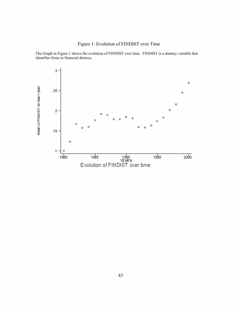
43

Figure 1: Evolution of FINDIST over Time

The Graph in Figure 1 shows the evolution of FINDIST over time. FINDIST is a dummy variable that identifies firms in financial distress.

44

Figure 2: Evolution of TCCGS and TRCA over time

The first graph in Figure 2 shows the evolution of TRCA and TCCGS (Trade Credit on Assets and Trade Credit on Cost of Goods Sold) over time. The second graph shows the evolution of the level of total assets and net sales of the firms over time. The time span is the same used in the regressions.

45

Figure 3: Evolution of the rate of growth of Assets and Sales

The Graphs in Figure 3 show the evolution of the growth rate of sales and assets and the TIMELINE. The growth rate of assets and sales are calculated using CPI-Adjusted levels of assets and sales. The horizontal line in the graphs represents the mean of the plotted variable in a sub-sample of firms that have TROUBLE=0. The vertical line represents the moment in which the firm entered in financial distress.

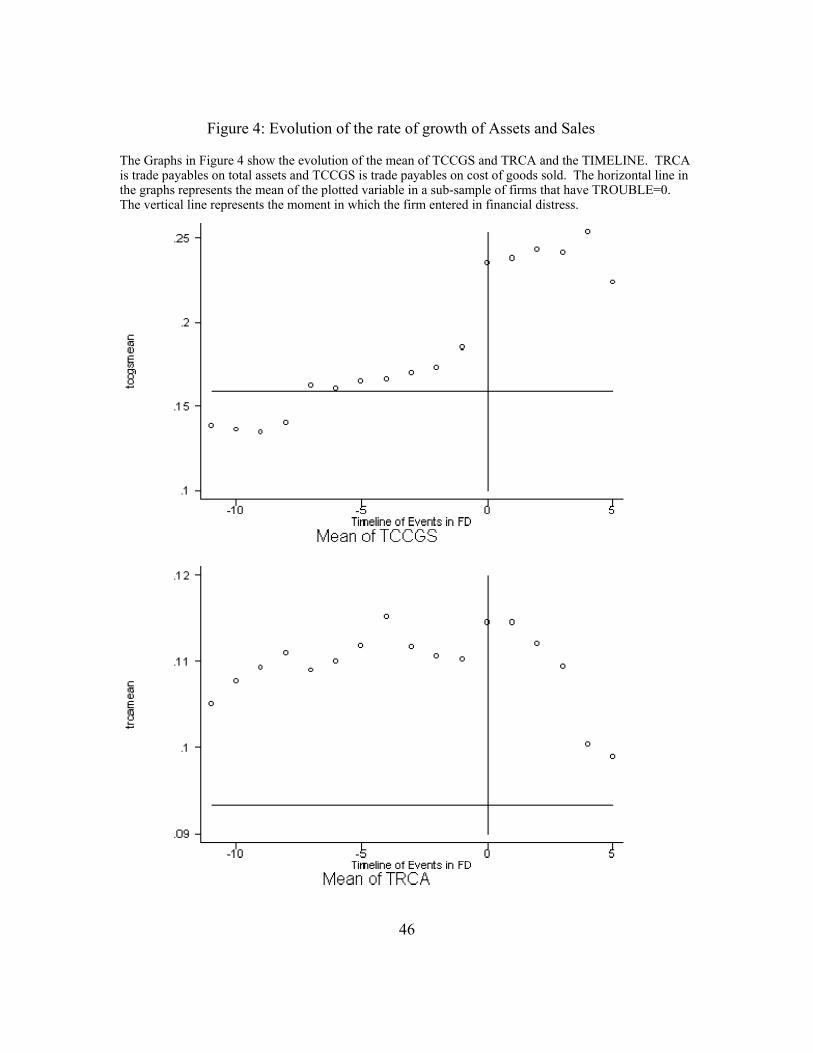
46

Figure 4: Evolution of the rate of growth of Assets and Sales

The Graphs in Figure 4 show the evolution of the mean of TCCGS and TRCA and the TIMELINE. TRCA is trade payables on total assets and TCCGS is trade payables on cost of goods sold. The horizontal line in the graphs represents the mean of the plotted variable in a sub-sample of firms that have TROUBLE=0. The vertical line represents the moment in which the firm entered in financial distress.

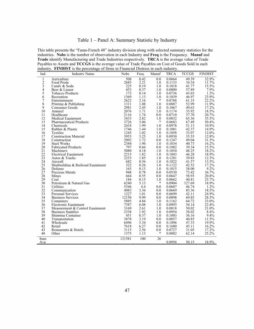
47

Table 1 – Panel A: Summary Statistic by Industry

This table presents the “Fama-French 48” industry division along with selected summary statistics for the industries. Nobs is the number of observation in each Industry and Freq is the Frequency. Manuf and Trade identify Manufacturing and Trade Industries respectively. TRCA is the average value of Trade Payables to Assets and TCCGS is the average value of Trade Payables on Cost of Goods Sold in each industry. FINDIST is the percentage of firms in Financial Distress in each industry.

Ind. Industry Name Nobs Freq. Manuf TRCA TCCGS FINDIST1 Agriculture 508 0.42 0.0 0.0664 49.39 32.9%2 Food Prods 2685 2.21 1.0 0.1133 34.34 11.7%3 Candy & Soda 225 0.19 1.0 0.1018 41.77 15.5%4 Beer & Liquor 453 0.37 1.0 0.0800 57.89 7.9%5 Tobacco Products 172 0.14 1.0 0.0736 43.65 1.3%6 Recreation 1369 1.13 1.0 0.1039 46.97 23.9%7 Entertainment 2622 2.16 * 0.0768 61.33 22.2%8 Printing & Publishing 1311 1.08 1.0 0.0887 52.99 11.9%9 Consumer Goods 2981 2.45 1.0 0.1067 49.63 17.2%10 Apparel 2076 1.71 1.0 0.1174 35.92 18.5%11 Healthcare 2116 1.74 0.0 0.0710 37.70 20.7%12 Medical Equipment 3433 2.82 1.0 0.0832 65.36 35.5%13 Pharmaceutical Products 3726 3.06 * 0.0683 67.49 50.4%14 Chemicals 2418 1.99 1.0 0.0978 51.13 10.9%15 Rubber & Plastic 1746 1.44 1.0 0.1081 42.37 14.9%16 Textiles 1245 1.02 1.0 0.1058 33.07 12.0%17 Construction Material 3953 3.25 1.0 0.0930 35.55 12.8%18 Construction 2092 1.72 0.0 0.1247 49.04 31.5%19 Steel Works 2384 1.96 1.0 0.1034 40.73 16.2%20 Fabricated Products 797 0.66 0.0 0.1082 39.34 15.5%21 Machinery 5080 4.18 1.0 0.1054 48.25 18.2%22 Electrical Equipment 2215 1.82 1.0 0.1043 46.28 18.9%23 Autos & Trucks 2253 1.85 1.0 0.1281 39.85 12.3%24 Aircraft 682 0.56 1.0 0.1022 41.57 13.5%25 Shipbuilding & Railroad Equipment 322 0.26 1.0 0.1122 42.52 17.2%26 Defense 163 0.13 1.0 0.1015 38.00 9.2%27 Precious Metals 948 0.78 0.0 0.0530 73.42 36.7%28 Mines 664 0.55 0.0 0.0647 58.93 20.8%29 Coal 184 0.15 1.0 0.0662 40.81 25.7%30 Petroleum & Natural Gas 6240 5.13 * 0.0904 127.69 18.9%31 Utilities 5346 4.4 0.0 0.0607 46.74 1.2%32 Communication 4083 3.36 0.0 0.0669 85.36 18.5%33 Personal Services 1227 1.01 0.0 0.0699 42.11 24.9%34 Business Services 12150 9.99 0.0 0.0898 69.85 28.5%35 Computers 5885 4.84 1.0 0.1162 64.72 33.0%36 Electronic Equipment 7387 6.08 1.0 0.0993 54.14 22.4%37 Measurement & Control Equipment 3169 2.61 1.0 0.0818 50.02 21.0%38 Business Supplies 2338 1.92 1.0 0.0954 38.02 8.4%39 Shipping Container 451 0.37 1.0 0.1003 36.16 9.4%40 Transportation 3878 3.19 0.0 0.0857 40.85 11.5%41 Wholesale 6496 5.34 0.0 0.1896 47.33 19.9%42 Retail 7618 6.27 0.0 0.1680 45.11 16.2%43 Restaurants & Hotels 3115 2.56 0.0 0.0727 31.05 17.2%48 Other 1375 1.13 * 0.0882 62.14 25.2%

Sum 121581 100 26 Avg 0.0956 50.15 18.9%

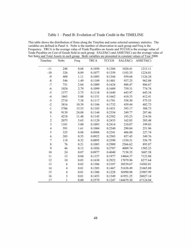
48

Table 1 – Panel B: Evolution of Trade Credit in the TIMELINE

This table shows the distribution of firms along the Timeline and some selected summary statistics. The variables are defined in Panel A. Nobs is the number of observation in each group and Freq is the Frequency. TRCA is the average value of Trade Payables on Assets and TCCGS is the average value of Trade Payables on Cost of Goods Sold in each group. SALES(C) and ASSETS(C) are the average value of Net Sales and Total Assets in each group. Both variables are presented in constant values of Year 2000.

Timeline Nobs Freq TRCA TCCGS SALES(C) ASSETS(C)

-11 248 0.68 0.1050 0.1384 1020.41 1213.11 -10 326 0.89 0.1077 0.1359 1103.35 1224.01 -9 409 1.11 0.1093 0.1344 959.68 1126.24 -8 546 1.49 0.1109 0.1401 937.25 962.08 -7 751 2.04 0.1089 0.1624 888.47 886.67 -6 1024 2.79 0.1099 0.1609 759.31 774.74 -5 1377 3.75 0.1118 0.1649 643.97 645.34 -4 1865 5.08 0.1151 0.1662 610.33 612.41 -3 2710 7.38 0.1117 0.1701 558.50 575.53 -2 3816 10.39 0.1106 0.1732 459.44 482.73 -1 5706 15.53 0.1103 0.1851 393.17 388.73 0 9139 24.88 0.1144 0.2354 249.77 287.46 1 4218 11.48 0.1145 0.2382 193.23 214.56 2 2075 5.65 0.1120 0.2435 162.03 203.48 3 1101 3.00 0.1093 0.2414 210.07 199.03 4 591 1.61 0.1004 0.2540 290.84 251.96 5 325 0.88 0.0988 0.2241 406.00 227.74 6 203 0.55 0.0922 0.2503 857.45 349.76 7 118 0.32 0.0895 0.2590 1330.31 556.79 8 76 0.21 0.1083 0.2909 2566.62 893.87 9 46 0.13 0.1056 0.2707 4009.74 1585.23

10 24 0.07 0.0977 0.4040 7158.35 3607.58 11 13 0.04 0.1157 0.1977 14864.37 7123.88 12 10 0.03 0.1630 0.2922 17079.96 8277.64 13 6 0.02 0.1306 0.2187 30539.67 14302.01 14 4 0.01 0.1303 0.1467 51638.49 21665.88 15 4 0.01 0.1306 0.1228 56990.98 23987.99 16 3 0.01 0.1453 0.1349 61951.25 26027.14 17 1 0.00 0.2579 0.1247 144479.30 67124.84

49

Table 2: Summary of the Main Variables

This table summarizes the main variables used in models of this paper. Measures of trade credit

TRCA trade payables over total assets

Measure what portion of the assets is financed by suppliers

TCCGS trade payables over cost of goods sold

Measures the trade credit (in days) scaled by the transaction that generated it (Purchases that is proxied by Cost of Goods Sold)

TCFD trade payables over financial debt

Measures the relation between trade credit and financial debt

TRCE trade payables over equity

Measures the relation between trade credit and equity

Measures of Distress

FINDIST FINDIST_LAG

Dummy Var. = 1 if the firm is in financial distress - (1 Lag). Alternative measure - 0 lags.

A firm is in FD if: EBITDA < Interest Pmts for two years in a row, Or, EBITDA < (80% * Interest Pmts) in any year

DEFAULT Dummy Var. = 1 if the firm is categorized in “default” by Standard &Poor’s

FDYS FDYS2

Number of years that a company has been in FD.

Sum of Years in which FINDIST = 1 for a given company.

TIMELINE Identifies at what stage of the financial distress process the company is

Zero indicates that the firm entered in financial distress in that same year. Positive numbers indicate the years spent in financial distress, and negative numbers indicate the distance to entering in financial distress.

TROUBLE Dummy variable = 1 if the firm has FINDIST=1 at any moment in the sample life

This variable indicates if the firm enters into financial distress at any time during the sample time.

Other Control Variables

SALESGROWTH Difference in sales from t-1 to t.

(Salest – Salest-1)/ Salest-1

MKTPOWER Measure of market power; interaction of market share, and Herfindahl Index.

Market share of firm * Herfindahl Index of industry

50

Table 3 – Panel A: Trade Credit and Financial Distress

This table shows the results of the estimation of Equations (1) and (2) for trade payables. The Dependent Variable is TCCGS, Trade Payables on Cost of Goods Sold. FINDIST_LAG is a dummy variable that is 1 if a firm is in financial distress under the measure by Asquith, Gertner and Scharfstein (1994) as defined in the paper and 0 otherwise. FDYS is a variable that counts how many years the firm has spent in Financial Distress. FDYS2 is FDYS squared. DIFSALES_SLES is the first difference in sales scaled by sales. LNASSETS is the natural log of total assets. The sample is the full sample form COMPUSTAT from 1980 to 2000. Absolute value of t-stats is shown in brackets. T-stats in the OLS specification are clustered by firms and are based on robust standard errors. All regressions have a constant that is not reported. Coefficients with *** are significant at 1% level, ** at 5%, and * at 10% in a two-tails test.

(1) (2) (3) (4) Dep. Var. TCCGS TCCGS TCCGS TCCGS

findist_lag 5.2121*** 3.7044*** 17.4823*** 10.5563*** [12.74] [8.13] [20.96] [13.71] difsales_sles 2.0532*** 2.4751*** 8.4794*** 9.5410*** [5.64] [6.69] [11.05] [12.35] fdys 1.1607*** 5.3299*** [4.36] [9.58] fdys2 0.0481 -0.3993*** [1.51] [4.86] lnassets 0.2532 0.3980* [1.16] [1.82] Observations 85733 85733 85733 85733 R-squared 0.7 0.7 0.15 0.15 Adj.R2 0.66 0.66 0.15 0.15 N firms 12018 12018 Model Fixed Effects Fixed Effects Pooled OLS Pooled OLS Sub-sample Full Sample Full Sample Full Sample Full Sample Dummies Firms Firms Industry Industry Clustering Firms Firms

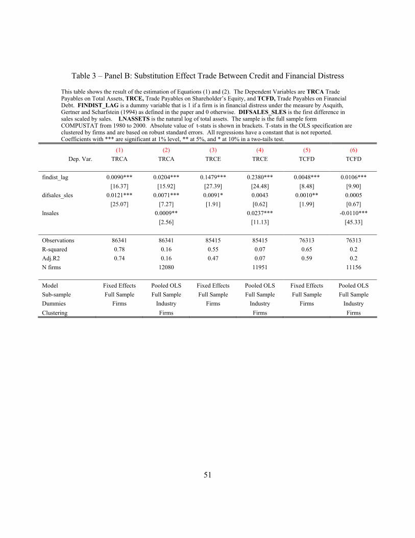
51

Table 3 – Panel B: Substitution Effect Trade Between Credit and Financial Distress

This table shows the result of the estimation of Equations (1) and (2). The Dependent Variables are TRCA Trade Payables on Total Assets, TRCE, Trade Payables on Shareholder’s Equity, and TCFD, Trade Payables on Financial Debt. FINDIST_LAG is a dummy variable that is 1 if a firm is in financial distress under the measure by Asquith, Gertner and Scharfstein (1994) as defined in the paper and 0 otherwise. DIFSALES_SLES is the first difference in sales scaled by sales. LNASSETS is the natural log of total assets. The sample is the full sample form COMPUSTAT from 1980 to 2000. Absolute value of t-stats is shown in brackets. T-stats in the OLS specification are clustered by firms and are based on robust standard errors. All regressions have a constant that is not reported. Coefficients with *** are significant at 1% level, ** at 5%, and * at 10% in a two-tails test.

(1) (2) (3) (4) (5) (6) Dep. Var. TRCA TRCA TRCE TRCE TCFD TCFD

findist_lag 0.0090*** 0.0204*** 0.1479*** 0.2380*** 0.0048*** 0.0106*** [16.37] [15.92] [27.39] [24.48] [8.48] [9.90] difsales_sles 0.0121*** 0.0071*** 0.0091* 0.0043 0.0010** 0.0005 [25.07] [7.27] [1.91] [0.62] [1.99] [0.67] lnsales 0.0009** 0.0237*** -0.0110*** [2.56] [11.13] [45.33] Observations 86341 86341 85415 85415 76313 76313 R-squared 0.78 0.16 0.55 0.07 0.65 0.2 Adj.R2 0.74 0.16 0.47 0.07 0.59 0.2 N firms 12080 11951 11156 Model Fixed Effects Pooled OLS Fixed Effects Pooled OLS Fixed Effects Pooled OLS Sub-sample Full Sample Full Sample Full Sample Full Sample Full Sample Full Sample Dummies Firms Industry Firms Industry Firms Industry Clustering Firms Firms Firms

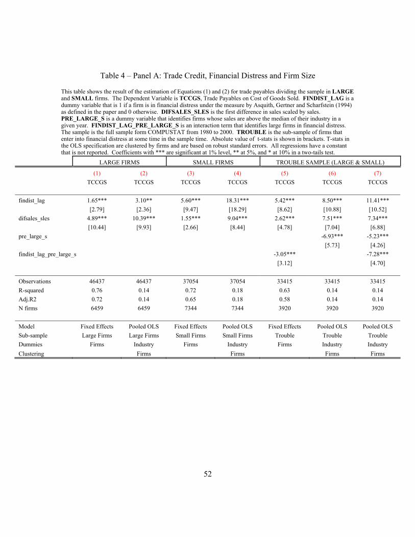
52

Table 4 – Panel A: Trade Credit, Financial Distress and Firm Size

This table shows the result of the estimation of Equations (1) and (2) for trade payables dividing the sample in LARGE and SMALL firms. The Dependent Variable is TCCGS, Trade Payables on Cost of Goods Sold. FINDIST_LAG is a dummy variable that is 1 if a firm is in financial distress under the measure by Asquith, Gertner and Scharfstein (1994) as defined in the paper and 0 otherwise. DIFSALES_SLES is the first difference in sales scaled by sales. PRE_LARGE_S is a dummy variable that identifies firms whose sales are above the median of their industry in a given year. FINDIST_LAG_PRE_LARGE_S is an interaction term that identifies large firms in financial distress. The sample is the full sample form COMPUSTAT from 1980 to 2000. TROUBLE is the sub-sample of firms that enter into financial distress at some time in the sample time. Absolute value of t-stats is shown in brackets. T-stats in the OLS specification are clustered by firms and are based on robust standard errors. All regressions have a constant that is not reported. Coefficients with *** are significant at 1% level, ** at 5%, and * at 10% in a two-tails test.

LARGE FIRMS SMALL FIRMS TROUBLE SAMPLE (LARGE & SMALL)

(1) (2) (3) (4) (5) (6) (7) TCCGS TCCGS TCCGS TCCGS TCCGS TCCGS TCCGS findist_lag 1.65*** 3.10** 5.60*** 18.31*** 5.42*** 8.50*** 11.41*** [2.79] [2.36] [9.47] [18.29] [8.62] [10.88] [10.52] difsales_sles 4.89*** 10.39*** 1.55*** 9.04*** 2.62*** 7.51*** 7.34*** [10.44] [9.93] [2.66] [8.44] [4.78] [7.04] [6.88] pre_large_s -6.93*** -5.23*** [5.73] [4.26] findist_lag_pre_large_s -3.05*** -7.28*** [3.12] [4.70] Observations 46437 46437 37054 37054 33415 33415 33415 R-squared 0.76 0.14 0.72 0.18 0.63 0.14 0.14 Adj.R2 0.72 0.14 0.65 0.18 0.58 0.14 0.14 N firms 6459 6459 7344 7344 3920 3920 3920 Model Fixed Effects Pooled OLS Fixed Effects Pooled OLS Fixed Effects Pooled OLS Pooled OLS Sub-sample Large Firms Large Firms Small Firms Small Firms Trouble Trouble Trouble Dummies Firms Industry Firms Industry Firms Industry Industry Clustering Firms Firms Firms Firms

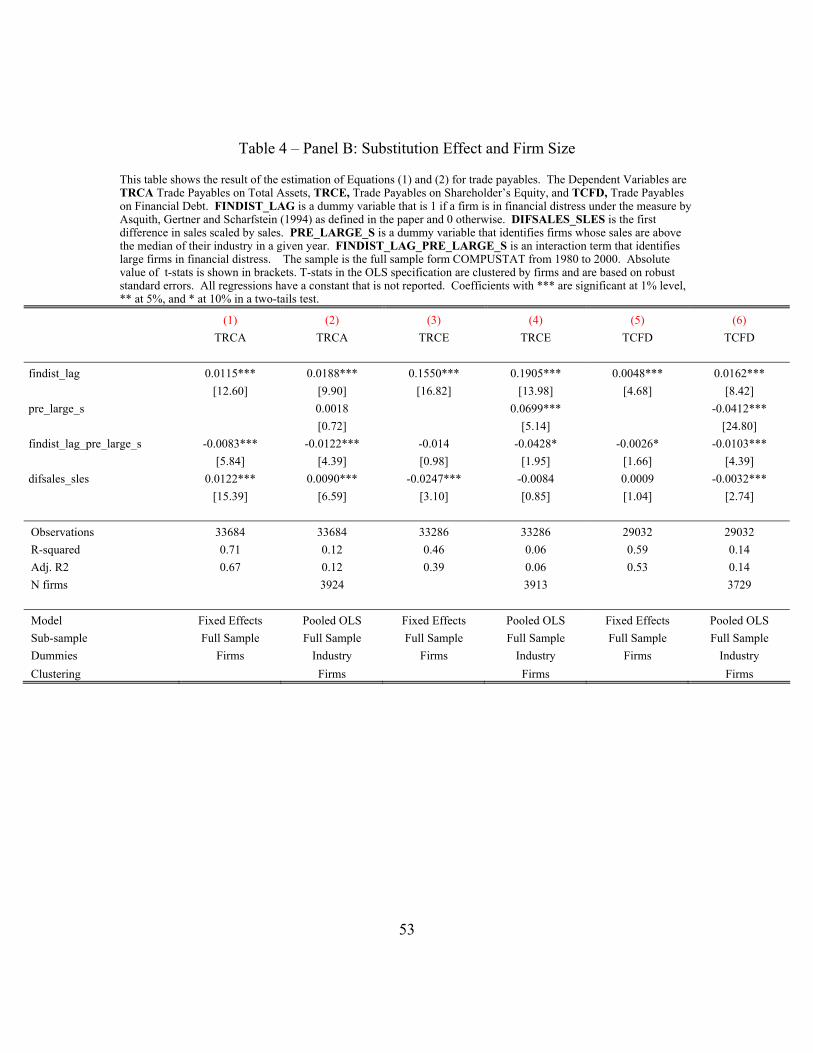
53

Table 4 – Panel B: Substitution Effect and Firm Size

This table shows the result of the estimation of Equations (1) and (2) for trade payables. The Dependent Variables are TRCA Trade Payables on Total Assets, TRCE, Trade Payables on Shareholder’s Equity, and TCFD, Trade Payables on Financial Debt. FINDIST_LAG is a dummy variable that is 1 if a firm is in financial distress under the measure by Asquith, Gertner and Scharfstein (1994) as defined in the paper and 0 otherwise. DIFSALES_SLES is the first difference in sales scaled by sales. PRE_LARGE_S is a dummy variable that identifies firms whose sales are above the median of their industry in a given year. FINDIST_LAG_PRE_LARGE_S is an interaction term that identifies large firms in financial distress. The sample is the full sample form COMPUSTAT from 1980 to 2000. Absolute value of t-stats is shown in brackets. T-stats in the OLS specification are clustered by firms and are based on robust standard errors. All regressions have a constant that is not reported. Coefficients with *** are significant at 1% level, ** at 5%, and * at 10% in a two-tails test.

(1) (2) (3) (4) (5) (6) TRCA TRCA TRCE TRCE TCFD TCFD findist_lag 0.0115*** 0.0188*** 0.1550*** 0.1905*** 0.0048*** 0.0162*** [12.60] [9.90] [16.82] [13.98] [4.68] [8.42] pre_large_s 0.0018 0.0699*** -0.0412*** [0.72] [5.14] [24.80] findist_lag_pre_large_s -0.0083*** -0.0122*** -0.014 -0.0428* -0.0026* -0.0103*** [5.84] [4.39] [0.98] [1.95] [1.66] [4.39] difsales_sles 0.0122*** 0.0090*** -0.0247*** -0.0084 0.0009 -0.0032*** [15.39] [6.59] [3.10] [0.85] [1.04] [2.74] Observations 33684 33684 33286 33286 29032 29032 R-squared 0.71 0.12 0.46 0.06 0.59 0.14 Adj. R2 0.67 0.12 0.39 0.06 0.53 0.14 N firms 3924 3913 3729 Model Fixed Effects Pooled OLS Fixed Effects Pooled OLS Fixed Effects Pooled OLS Sub-sample Full Sample Full Sample Full Sample Full Sample Full Sample Full Sample Dummies Firms Industry Firms Industry Firms Industry Clustering Firms Firms Firms

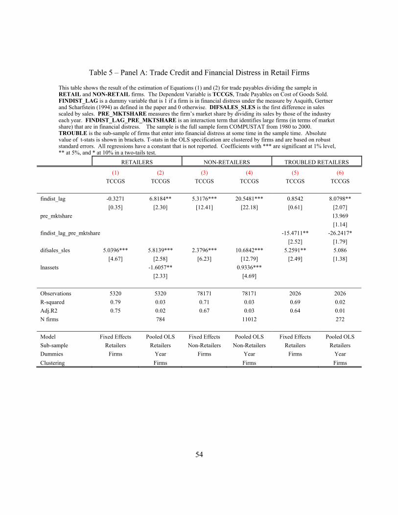
54

Table 5 – Panel A: Trade Credit and Financial Distress in Retail Firms

This table shows the result of the estimation of Equations (1) and (2) for trade payables dividing the sample in RETAIL and NON-RETAIL firms. The Dependent Variable is TCCGS, Trade Payables on Cost of Goods Sold. FINDIST_LAG is a dummy variable that is 1 if a firm is in financial distress under the measure by Asquith, Gertner and Scharfstein (1994) as defined in the paper and 0 otherwise. DIFSALES_SLES is the first difference in sales scaled by sales. PRE_MKTSHARE measures the firm’s market share by dividing its sales by those of the industry each year. FINDIST_LAG_PRE_MKTSHARE is an interaction term that identifies large firms (in terms of market share) that are in financial distress. The sample is the full sample form COMPUSTAT from 1980 to 2000. TROUBLE is the sub-sample of firms that enter into financial distress at some time in the sample time. Absolute value of t-stats is shown in brackets. T-stats in the OLS specification are clustered by firms and are based on robust standard errors. All regressions have a constant that is not reported. Coefficients with *** are significant at 1% level, ** at 5%, and * at 10% in a two-tails test.

RETAILERS NON-RETAILERS TROUBLED RETAILERS

(1) (2) (3) (4) (5) (6) TCCGS TCCGS TCCGS TCCGS TCCGS TCCGS findist_lag -0.3271 6.8184** 5.3176*** 20.5481*** 0.8542 8.0798** [0.35] [2.30] [12.41] [22.18] [0.61] [2.07] pre_mktshare 13.969 [1.14] findist_lag_pre_mktshare -15.4711** -26.2417* [2.52] [1.79] difsales_sles 5.0396*** 5.8139*** 2.3796*** 10.6842*** 5.2591** 5.086 [4.67] [2.58] [6.23] [12.79] [2.49] [1.38] lnassets -1.6057** 0.9336*** [2.33] [4.69] Observations 5320 5320 78171 78171 2026 2026 R-squared 0.79 0.03 0.71 0.03 0.69 0.02 Adj.R2 0.75 0.02 0.67 0.03 0.64 0.01 N firms 784 11012 272 Model Fixed Effects Pooled OLS Fixed Effects Pooled OLS Fixed Effects Pooled OLS Sub-sample Retailers Retailers Non-Retailers Non-Retailers Retailers Retailers Dummies Firms Year Firms Year Firms Year Clustering Firms Firms Firms

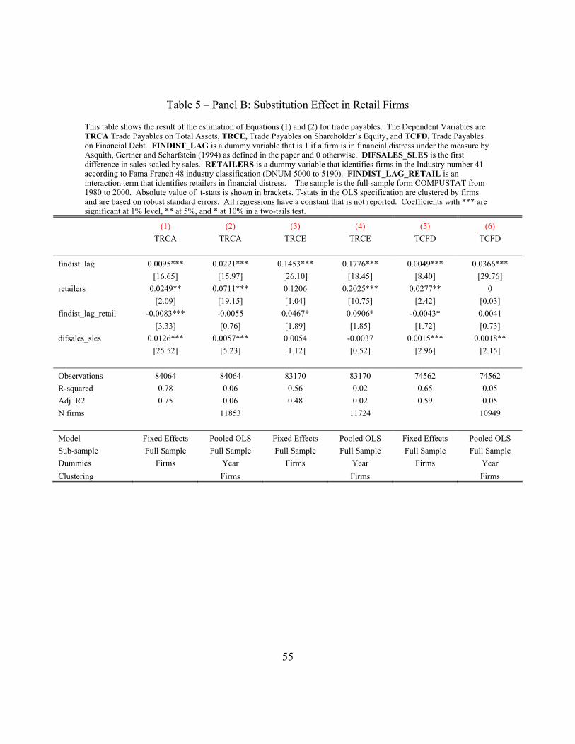
55

Table 5 – Panel B: Substitution Effect in Retail Firms

This table shows the result of the estimation of Equations (1) and (2) for trade payables. The Dependent Variables are TRCA Trade Payables on Total Assets, TRCE, Trade Payables on Shareholder’s Equity, and TCFD, Trade Payables on Financial Debt. FINDIST_LAG is a dummy variable that is 1 if a firm is in financial distress under the measure by Asquith, Gertner and Scharfstein (1994) as defined in the paper and 0 otherwise. DIFSALES_SLES is the first difference in sales scaled by sales. RETAILERS is a dummy variable that identifies firms in the Industry number 41 according to Fama French 48 industry classification (DNUM 5000 to 5190). FINDIST_LAG_RETAIL is an interaction term that identifies retailers in financial distress. The sample is the full sample form COMPUSTAT from 1980 to 2000. Absolute value of t-stats is shown in brackets. T-stats in the OLS specification are clustered by firms and are based on robust standard errors. All regressions have a constant that is not reported. Coefficients with *** are significant at 1% level, ** at 5%, and * at 10% in a two-tails test.

(1) (2) (3) (4) (5) (6) TRCA TRCA TRCE TRCE TCFD TCFD findist_lag 0.0095*** 0.0221*** 0.1453*** 0.1776*** 0.0049*** 0.0366*** [16.65] [15.97] [26.10] [18.45] [8.40] [29.76] retailers 0.0249** 0.0711*** 0.1206 0.2025*** 0.0277** 0 [2.09] [19.15] [1.04] [10.75] [2.42] [0.03] findist_lag_retail -0.0083*** -0.0055 0.0467* 0.0906* -0.0043* 0.0041 [3.33] [0.76] [1.89] [1.85] [1.72] [0.73] difsales_sles 0.0126*** 0.0057*** 0.0054 -0.0037 0.0015*** 0.0018** [25.52] [5.23] [1.12] [0.52] [2.96] [2.15] Observations 84064 84064 83170 83170 74562 74562 R-squared 0.78 0.06 0.56 0.02 0.65 0.05 Adj. R2 0.75 0.06 0.48 0.02 0.59 0.05 N firms 11853 11724 10949 Model Fixed Effects Pooled OLS Fixed Effects Pooled OLS Fixed Effects Pooled OLS Sub-sample Full Sample Full Sample Full Sample Full Sample Full Sample Full Sample Dummies Firms Year Firms Year Firms Year Clustering Firms Firms Firms

56

Table 6 – Panel A: Trade Credit and Financial Distress in Manufacturing Firms

This table shows the result of the estimation of Equations (1) and (2) for trade payables. The Dependent Variable is TCCGS, Trade Payables on Cost of Goods Sold. FINDIST_LAG is a dummy variable that is 1 if a firm is in financial distress under the measure by Asquith, Gertner and Scharfstein (1994) as defined in the paper and 0 otherwise. DIFSALES_SLES is the first difference in sales scaled by sales. MANUF is a dummy variable that identifies manufacturing firms as defined in Table 1. FINDIST_LAG_MANUF is an interaction term that identifies manufacturing firms in financial distress. The sample is the sub-sample of firms in TROUBLE form COMPUSTAT from 1980 to 2000. TROUBLE is the sub-sample of firms that enter into financial distress at some time in the sample time. Absolute value of t-stats is shown in brackets. T-stats in the OLS specification are clustered by firms and are based on robust standard errors. All regressions have a constant that is not reported. Coefficients with *** are significant at 1% level, ** at 5%, and * at 10% in a two-tails test.

(1) (2) (3) TCCGS TCCGS TCCGS findist_lag 5.9143*** 17.4788*** 16.6814*** [9.44] [20.73] [11.18] manuf -4.0501 -25.9796*** -26.2975*** [1.33] [5.57] [5.58] findist_lag_manuf -1.5601* 1.5025 [1.90] [0.83] difsales_sles 2.4928*** 9.0018*** 9.0190*** [6.80] [11.59] [11.61] lnassets 0.5342** 0.5372** [2.54] [2.55] Observations 83491 83491 83491 R-squared 0.71 0.16 0.16 Adj. R2 0.67 0.16 0.16 N firms 11791 11791 Model Fixed Effects Pooled OLS Pooled OLS Sub-sample Trouble Trouble Trouble Dummies Firms Year Year Clustering Firms Firms

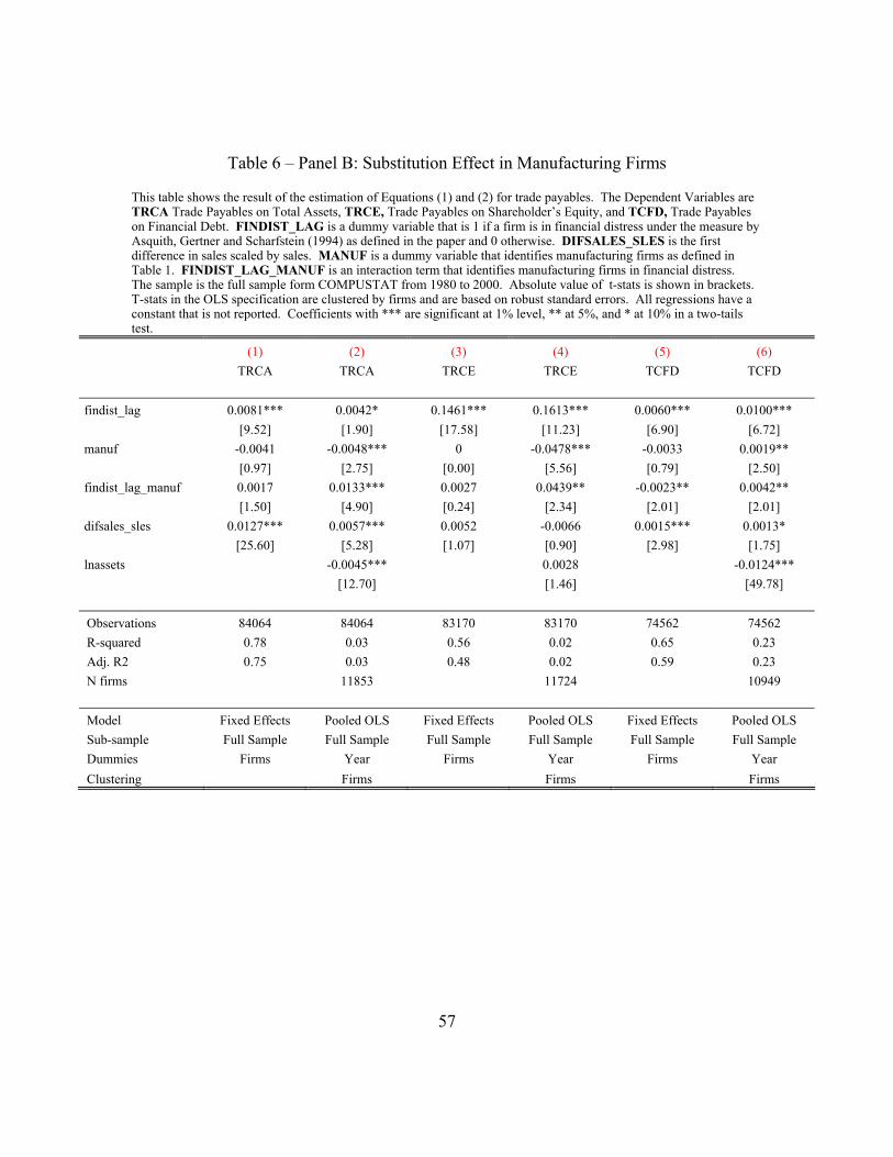
57

Table 6 – Panel B: Substitution Effect in Manufacturing Firms

This table shows the result of the estimation of Equations (1) and (2) for trade payables. The Dependent Variables are TRCA Trade Payables on Total Assets, TRCE, Trade Payables on Shareholder’s Equity, and TCFD, Trade Payables on Financial Debt. FINDIST_LAG is a dummy variable that is 1 if a firm is in financial distress under the measure by Asquith, Gertner and Scharfstein (1994) as defined in the paper and 0 otherwise. DIFSALES_SLES is the first difference in sales scaled by sales. MANUF is a dummy variable that identifies manufacturing firms as defined in Table 1. FINDIST_LAG_MANUF is an interaction term that identifies manufacturing firms in financial distress. The sample is the full sample form COMPUSTAT from 1980 to 2000. Absolute value of t-stats is shown in brackets. T-stats in the OLS specification are clustered by firms and are based on robust standard errors. All regressions have a constant that is not reported. Coefficients with *** are significant at 1% level, ** at 5%, and * at 10% in a two-tails test.

(1) (2) (3) (4) (5) (6) TRCA TRCA TRCE TRCE TCFD TCFD findist_lag 0.0081*** 0.0042* 0.1461*** 0.1613*** 0.0060*** 0.0100*** [9.52] [1.90] [17.58] [11.23] [6.90] [6.72] manuf -0.0041 -0.0048*** 0 -0.0478*** -0.0033 0.0019** [0.97] [2.75] [0.00] [5.56] [0.79] [2.50] findist_lag_manuf 0.0017 0.0133*** 0.0027 0.0439** -0.0023** 0.0042** [1.50] [4.90] [0.24] [2.34] [2.01] [2.01] difsales_sles 0.0127*** 0.0057*** 0.0052 -0.0066 0.0015*** 0.0013* [25.60] [5.28] [1.07] [0.90] [2.98] [1.75] lnassets -0.0045*** 0.0028 -0.0124*** [12.70] [1.46] [49.78] Observations 84064 84064 83170 83170 74562 74562 R-squared 0.78 0.03 0.56 0.02 0.65 0.23 Adj. R2 0.75 0.03 0.48 0.02 0.59 0.23 N firms 11853 11724 10949 Model Fixed Effects Pooled OLS Fixed Effects Pooled OLS Fixed Effects Pooled OLS Sub-sample Full Sample Full Sample Full Sample Full Sample Full Sample Full Sample Dummies Firms Year Firms Year Firms Year Clustering Firms Firms Firms

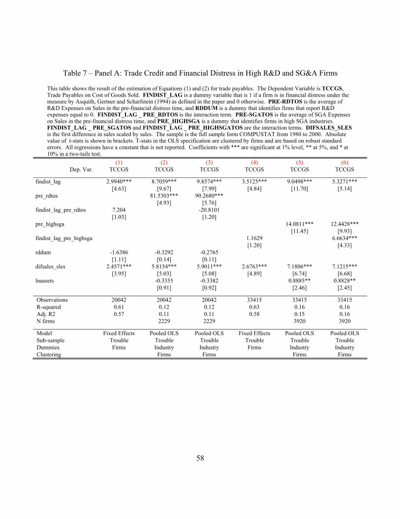
58

Table 7 – Panel A: Trade Credit and Financial Distress in High R&D and SG&A Firms

This table shows the result of the estimation of Equations (1) and (2) for trade payables. The Dependent Variable is TCCGS, Trade Payables on Cost of Goods Sold. FINDIST_LAG is a dummy variable that is 1 if a firm is in financial distress under the measure by Asquith, Gertner and Scharfstein (1994) as defined in the paper and 0 otherwise. PRE-RDTOS is the average of R&D Expenses on Sales in the pre-financial distress time, and RDDUM is a dummy that identifies firms that report R&D expenses equal to 0. FINDIST_LAG _ PRE_RDTOS is the interaction term. PRE-SGATOS is the average of SGA Expenses on Sales in the pre-financial distress time, and PRE_HIGHSGA is a dummy that identifies firms in high SGA industries. FINDIST_LAG _ PRE_SGATOS and FINDIST_LAG _ PRE_HIGHSGATOS are the interaction terms. DIFSALES_SLES is the first difference in sales scaled by sales. The sample is the full sample form COMPUSTAT from 1980 to 2000. Absolute value of t-stats is shown in brackets. T-stats in the OLS specification are clustered by firms and are based on robust standard errors. All regressions have a constant that is not reported. Coefficients with *** are significant at 1% level, ** at 5%, and * at 10% in a two-tails test.

(1) (2) (3) (4) (5) (6) Dep. Var. TCCGS TCCGS TCCGS TCCGS TCCGS TCCGS

findist_lag 2.9940*** 8.7059*** 9.8574*** 3.5125*** 9.0498*** 5.3271*** [4.63] [9.67] [7.99] [4.84] [11.70] [5.14] pre_rdtos 81.5303*** 90.2680*** [4.93] [5.76] findist_lag_pre_rdtos 7.204 -20.8101 [1.03] [1.20] pre_highsga 14.0811*** 12.4428*** [11.45] [9.93] findist_lag_pre_highsga 1.1629 6.6634*** [1.20] [4.33] rddum -1.6386 -0.3292 -0.2765 [1.11] [0.14] [0.11] difsales_sles 2.4571*** 5.8154*** 5.9011*** 2.6763*** 7.1806*** 7.1215*** [3.95] [5.03] [5.08] [4.89] [6.74] [6.68] lnassets -0.3355 -0.3382 0.8885** 0.8828** [0.91] [0.92] [2.46] [2.45]

Observations 20042 20042 20042 33415 33415 33415 R-squared 0.61 0.12 0.12 0.63 0.16 0.16 Adj. R2 0.57 0.11 0.11 0.58 0.15 0.16 N firms 2229 2229 3920 3920

Model Fixed Effects Pooled OLS Pooled OLS Fixed Effects Pooled OLS Pooled OLS Sub-sample Trouble Trouble Trouble Trouble Trouble Trouble Dummies Firms Industry Industry Firms Industry Industry Clustering Firms Firms Firms Firms

59

Table 7 – Panel B: Substitution Effect in High R&D Firms

This table shows the result of the estimation of Equations (1) and (2) for trade payables. The Dependent Variables are TRCA Trade Payables on Total Assets, TRCE, Trade Payables on Shareholder’s Equity, and TCFD, Trade Payables on Financial Debt. FINDIST_LAG is a dummy variable that is 1 if a firm is in financial distress under the measure by Asquith, Gertner and Scharfstein (1994) as defined in the paper and 0 otherwise. PRE-RDTOS is the average of R&D Expenses on Sales in the pre-financial distress time, and RDDUM is a dummy that identifies firms that report R&D expenses equal to 0. FINDIST_LAG _ PRE_RDTOS is the interaction term. DIFSALES_SLES is the first difference in sales scaled by sales. The sample is the full sample form COMPUSTAT from 1980 to 2000. Absolute value of t-stats is shown in brackets. T-stats in the OLS specification are clustered by firms and are based on robust standard errors. All regressions have a constant that is not reported. Coefficients with *** are significant at 1% level, ** at 5%, and * at 10% in a two-tails test.

(1) (2) (3) (4) (5) (6) Dep. Var. TRCA TRCA TRCE TRCE TCFD TCFD

findist_lag 0.0075*** 0.0116*** 0.1516*** 0.1791*** 0.0009 0.002 [7.00] [5.54] [14.46] [11.40] [0.70] [1.10] pre_rdtos -0.2000*** -0.9060*** 0.0224 [10.34] [9.42] [1.32] findist_lag_pre_rdtos 0.0225* 0.0679*** -0.3162*** -0.031 0.0293* 0.0078 [1.94] [3.61] [2.82] [0.28] [1.87] [0.37] rddum -0.0032 0.0183*** -0.0683*** 0.058 0.0082*** 0.0008 [1.29] [2.78] [2.86] [1.62] [2.74] [0.19] difsales_sles 0.0133*** 0.0105*** -0.0193* -0.0218* 0.0038*** 0.0062*** [12.90] [5.79] [1.93] [1.65] [2.90] [3.63] lnsales 0.0007 0.0306*** -0.0187*** [0.80] [6.01] [24.29] Observations 20111 20111 19904 19904 16890 16890 R-squared 0.7 0.17 0.44 0.09 0.57 0.2 Adj. R2 0.66 0.17 0.37 0.09 0.51 0.2 N firms 2229 2226 2102 Model Fixed Effects Pooled OLS Fixed Effects Pooled OLS Fixed Effects Pooled OLS Sub-sample Trouble Trouble Trouble Trouble Trouble Trouble Dummies Firms Industry Firms Industry Firms Industry Clustering Firms Firms Firms

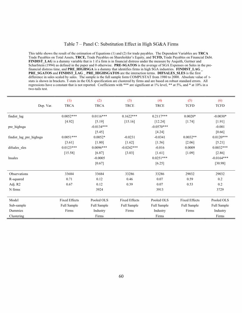
60

Table 7 – Panel C: Substitution Effect in High SG&A Firms

This table shows the result of the estimation of Equations (1) and (2) for trade payables. The Dependent Variables are TRCA Trade Payables on Total Assets, TRCE, Trade Payables on Shareholder’s Equity, and TCFD, Trade Payables on Financial Debt. FINDIST_LAG is a dummy variable that is 1 if a firm is in financial distress under the measure by Asquith, Gertner and Scharfstein (1994) as defined in the paper and 0 otherwise. PRE-SGATOS is the average of SGA Expenses on Sales in the pre-financial distress time, and PRE_HIGHSGA is a dummy that identifies firms in high SGA industries. FINDIST_LAG _ PRE_SGATOS and FINDIST_LAG _ PRE_HIGHSGATOS are the interaction terms. DIFSALES_SLES is the first difference in sales scaled by sales. The sample is the full sample form COMPUSTAT from 1980 to 2000. Absolute value of t-stats is shown in brackets. T-stats in the OLS specification are clustered by firms and are based on robust standard errors. All regressions have a constant that is not reported. Coefficients with *** are significant at 1% level, ** at 5%, and * at 10% in a two-tails test.

(1) (2) (3) (4) (5) (6)

Dep. Var. TRCA TRCA TRCE TRCE TCFD TCFD

findist_lag 0.0052*** 0.0116*** 0.1622*** 0.2117*** 0.0020* -0.0030* [4.92] [5.19] [15.16] [12.24] [1.74] [1.91] pre_highsga -0.0134*** -0.0570*** -0.001 [5.45] [4.24] [0.66] findist_lag_pre_highsga 0.0051*** 0.0052* -0.0231 -0.0341 0.0032** 0.0120*** [3.61] [1.80] [1.62] [1.56] [2.06] [5.21] difsales_sles 0.0123*** 0.0096*** -0.0242*** -0.016 0.0009 0.0032*** [15.58] [6.87] [3.03] [1.61] [1.09] [2.86] lnsales -0.0005 0.0251*** -0.0164*** [0.67] [6.25] [30.98] Observations 33684 33684 33286 33286 29032 29032 R-squared 0.71 0.12 0.46 0.07 0.59 0.2 Adj. R2 0.67 0.12 0.39 0.07 0.53 0.2 N firms 3924 3913 3729 Model Fixed Effects Pooled OLS Fixed Effects Pooled OLS Fixed Effects Pooled OLS Sub-sample Full Sample Full Sample Full Sample Full Sample Full Sample Full Sample Dummies Firms Industry Firms Industry Firms Industry Clustering Firms Firms Firms

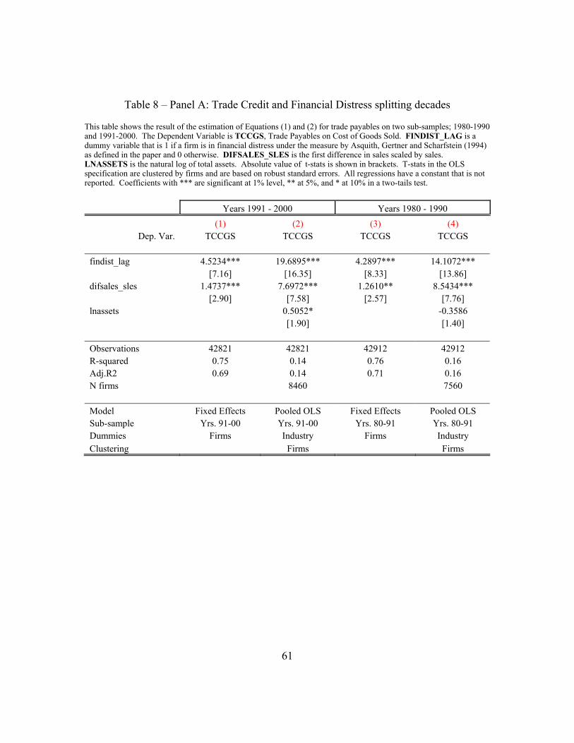
61

Table 8 – Panel A: Trade Credit and Financial Distress splitting decades

This table shows the result of the estimation of Equations (1) and (2) for trade payables on two sub-samples; 1980-1990 and 1991-2000. The Dependent Variable is TCCGS, Trade Payables on Cost of Goods Sold. FINDIST_LAG is a dummy variable that is 1 if a firm is in financial distress under the measure by Asquith, Gertner and Scharfstein (1994) as defined in the paper and 0 otherwise. DIFSALES_SLES is the first difference in sales scaled by sales. LNASSETS is the natural log of total assets. Absolute value of t-stats is shown in brackets. T-stats in the OLS specification are clustered by firms and are based on robust standard errors. All regressions have a constant that is not reported. Coefficients with *** are significant at 1% level, ** at 5%, and * at 10% in a two-tails test.

Years 1991 - 2000 Years 1980 - 1990 (1) (2) (3) (4)

Dep. Var. TCCGS TCCGS TCCGS TCCGS findist_lag 4.5234*** 19.6895*** 4.2897*** 14.1072*** [7.16] [16.35] [8.33] [13.86] difsales_sles 1.4737*** 7.6972*** 1.2610** 8.5434*** [2.90] [7.58] [2.57] [7.76] lnassets 0.5052* -0.3586 [1.90] [1.40] Observations 42821 42821 42912 42912 R-squared 0.75 0.14 0.76 0.16 Adj.R2 0.69 0.14 0.71 0.16 N firms 8460 7560 Model Fixed Effects Pooled OLS Fixed Effects Pooled OLS Sub-sample Yrs. 91-00 Yrs. 91-00 Yrs. 80-91 Yrs. 80-91 Dummies Firms Industry Firms Industry Clustering Firms Firms

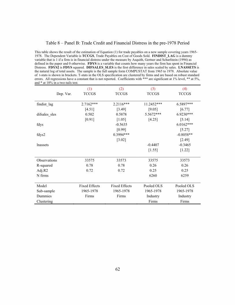
62

Table 8 – Panel B: Trade Credit and Financial Distress in the pre-1978 Period

This table shows the result of the estimation of Equation (1) for trade payables on a new sample covering years 1965-1978. The Dependent Variable is TCCGS, Trade Payables on Cost of Goods Sold. FINDIST_LAG is a dummy variable that is 1 if a firm is in financial distress under the measure by Asquith, Gertner and Scharfstein (1994) as defined in the paper and 0 otherwise. FDYS is a variable that counts how many years the firm has spent in Financial Distress. FDYS2 is FDYS squared. DIFSALES_SLES is the first difference in sales scaled by sales. LNASSETS is the natural log of total assets. The sample is the full sample form COMPUSTAT from 1965 to 1978. Absolute value of t-stats is shown in brackets. T-stats in the OLS specification are clustered by firms and are based on robust standard errors. All regressions have a constant that is not reported. Coefficients with *** are significant at 1% level, ** at 5%, and * at 10% in a two-tails test.

(1) (2) (3) (4) Dep. Var. TCCGS TCCGS TCCGS TCCGS

findist_lag 2.7162*** 2.2116*** 11.2452*** 6.5897*** [4.51] [3.49] [9.05] [6.77] difsales_sles 0.502 0.5878 5.5672*** 6.9230*** [0.91] [1.05] [4.25] [5.14] fdys -0.5635 6.0162*** [0.99] [5.27] fdys2 0.3994*** -0.8058** [3.02] [2.49] lnassets -0.4407 -0.3465 [1.55] [1.22] Observations 33575 33573 33575 33573 R-squared 0.78 0.78 0.26 0.26 Adj.R2 0.72 0.72 0.25 0.25 N firms 6260 6259 Model Fixed Effects Fixed Effects Pooled OLS Pooled OLS Sub-sample 1965-1978 1965-1978 1965-1978 1965-1978 Dummies Firms Firms Industry Industry Clustering Firms Firms

63

Table 9 – Panel A: Trade Credit and Financial (not Economic) Distress

This table shows the results of the estimation of Equations (1) and (2) for trade payables. The Dependent Variable is TCCGS, Trade Payables on Cost of Goods Sold. FDLEV is a dummy variable that is 1 if a firm is in financial distress as defined in Table 3 and its leverage is in the top two deciles of its industry. DIFSALES_SLES is the first difference in sales scaled by sales. LNASSETS is the natural log of total assets. The sample is the full sample form COMPUSTAT from 1980 to 2000. Absolute value of t-stats is shown in brackets. T-stats in the OLS specification are clustered by firms and are based on robust standard errors. All regressions have a constant that is not reported. Coefficients with *** are significant at 1% level, ** at 5%, and * at 10% in a two-tails test.

(1) (2) (3) (4) Dep. Var. TCCGS TCCGS TCCGS TCCGS

fdlev 2.6381*** 13.2435*** [4.81] [13.23] fdlev_lag 2.5970*** 10.7902*** [4.35] [9.96] difsales_sles 2.4794*** 11.0106*** 2.1675*** 9.6952*** [7.33] [15.59] [5.96] [12.58] lnassets -0.8320*** -0.5679*** [4.03] [2.63] Observations 97786 97786 85548 85548 R-squared 0.69 0.14 0.7 0.14 Adj.R2 0.64 0.14 0.65 0.14 N firms 13389 12002 Model Fixed Effects Pooled OLS Fixed Effects Pooled OLS Sub-sample Full Sample Full Sample Full Sample Full Sample Dummies Firms Industry Firms Industry Clustering Firms Firms

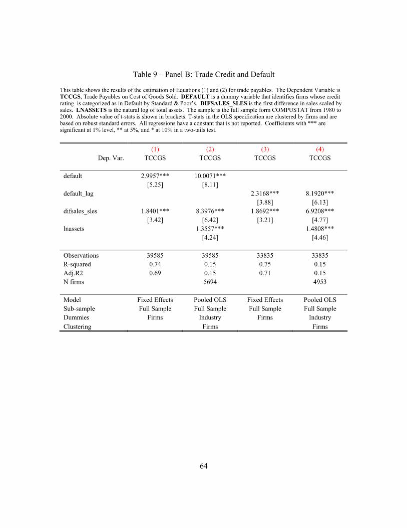
64

Table 9 – Panel B: Trade Credit and Default

This table shows the results of the estimation of Equations (1) and (2) for trade payables. The Dependent Variable is TCCGS, Trade Payables on Cost of Goods Sold. DEFAULT is a dummy variable that identifies firms whose credit rating is categorized as in Default by Standard & Poor’s. DIFSALES_SLES is the first difference in sales scaled by sales. LNASSETS is the natural log of total assets. The sample is the full sample form COMPUSTAT from 1980 to 2000. Absolute value of t-stats is shown in brackets. T-stats in the OLS specification are clustered by firms and are based on robust standard errors. All regressions have a constant that is not reported. Coefficients with *** are significant at 1% level, ** at 5%, and * at 10% in a two-tails test.

(1) (2) (3) (4) Dep. Var. TCCGS TCCGS TCCGS TCCGS

default 2.9957*** 10.0071*** [5.25] [8.11] default_lag 2.3168*** 8.1920*** [3.88] [6.13] difsales_sles 1.8401*** 8.3976*** 1.8692*** 6.9208*** [3.42] [6.42] [3.21] [4.77] lnassets 1.3557*** 1.4808*** [4.24] [4.46] Observations 39585 39585 33835 33835 R-squared 0.74 0.15 0.75 0.15 Adj.R2 0.69 0.15 0.71 0.15 N firms 5694 4953 Model Fixed Effects Pooled OLS Fixed Effects Pooled OLS Sub-sample Full Sample Full Sample Full Sample Full Sample Dummies Firms Industry Firms Industry Clustering Firms Firms

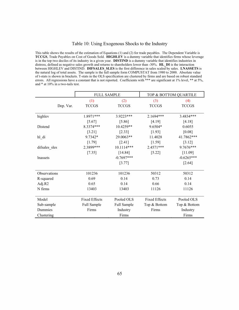
65

Table 10: Using Exogenous Shocks to the Industry

This table shows the results of the estimation of Equations (1) and (2) for trade payables. The Dependent Variable is TCCGS, Trade Payables on Cost of Goods Sold. HIGHLEV is a dummy variable that identifies firms whose leverage is in the top two deciles of its industry in a given year. DISTIND is a dummy variable that identifies industries in distress, defined as negative sales growth and returns to shareholders lower than -30%. HL_DI is the interaction between HIGHLEV and DISTIND. DIFSALES_SLES is the first difference in sales scaled by sales. LNASSETS is the natural log of total assets. The sample is the full sample form COMPUSTAT from 1980 to 2000. Absolute value of t-stats is shown in brackets. T-stats in the OLS specification are clustered by firms and are based on robust standard errors. All regressions have a constant that is not reported. Coefficients with *** are significant at 1% level, ** at 5%, and * at 10% in a two-tails test.

FULL SAMPLE TOP & BOTTOM QUARTILE (1) (2) (3) (4)

Dep. Var. TCCGS TCCGS TCCGS TCCGS highlev 1.8971*** 3.9223*** 2.1694*** 3.4834*** [5.67] [5.86] [4.19] [4.18] Distend 8.3374*** 10.4259** 9.6504* 0.6055 [3.21] [2.33] [1.93] [0.08] hl_di 9.7342* 29.0063** 11.4028 41.7862*** [1.79] [2.41] [1.59] [3.12] difsales_sles 2.3899*** 10.1114*** 2.4571*** 9.7676*** [7.35] [14.84] [5.22] [11.09] lnassets -0.7697*** -0.6265*** [3.77] [2.64] Observations 101236 101236 50312 50312 R-squared 0.69 0.14 0.73 0.14 Adj.R2 0.65 0.14 0.66 0.14 N firms 13403 13403 11126 11126 Model Fixed Effects Pooled OLS Fixed Effects Pooled OLS Sub-sample Full Sample Full Sample Top & Bottom Top & Bottom Dummies Firms Industry Firms Industry Clustering Firms Firms