1

An Empirical Analysis of County-Level Determinants of Small Business Growth Poverty in Appalachia: A Spatial Simultaneous-Equations Approach

Gebremeskel H. Gebremariam, Graduate Research Assistant

Tesfa G. Gebremedhin, Professor

Peter V. Schaeffer, Professor and Director

Division of Resource Management Davis College of Agriculture, Forestry & Consumer Sciences

P. O. Box 6108 West Virginia University

Morgantown, WV 26506-6108

Selected Paper prepared for presentation at the annual meeting of the Southern Agricultural

Economics Association in Orlando, Florida, on February 5-8, 2006.

Copyright 2006 by Gebremeskel Gebremariam, Tesfa Gebremedhin and Peter Schaeffer. All

rights reserved. Readers may make verbatim copies of this document for non-commercial

purposes by any means, provided that this copyright notice appears on all such copies.

2

An Empirical Analysis of County-Level Determinants of Small Business Growth Poverty in Appalachia: A Spatial Simultaneous-Equations Approach

1. Introduction

Persistent poverty is one of the most critical social problems facing policy makers in the

United States. Despite decades of government intervention, and the spending of billions of public

funds, many communities still remain in poverty. The economic boom of the 1990s not only

failed to reduce poverty in all counties, but it was associated with rising poverty rates in certain

counties (Rupasingha and Goetz, 2003). Counties in the Appalachia, for example, had above

average poverty rates in 1990s. Thus, after a decade of unprecedented expansion of the economy

of the United States, many regions in the Appalachia are still suffering from high unemployment,

shrinking economic base, deeply rooted poverty, low human capital formation, and out migration

(Deavers and Hoppe, 1992; Haynes, 1997; Dilger and Witt, 1994; Maggar, 1990). The slow

growth of income and employment in the region, out-migration and the disappearance of rural

households are both causes and effects of persistent high rates of poverty. This lagging economic

development negatively affect the economic and social well-being of the rural population, the

health of local businesses, and the ability of local governments to provide basic human services

(Cushing and Rogers, 1996).

The changing structure of traditional industries and the impact of those changes on local

communities have been sources of concern to many groups interested in the welfare of rural

areas. State policy makers and local leaders have been placing a high priority on local economic

development (Pulver, 1989; Ekstrom and Leistritz, 1988). Consequently, a better understanding

of factors that influence the local employment earning capacity and quality of life issues has

become important from county, state and regional policy perspectives with respect to designing

human capital development programs needed for rural community development. Since many of

the forces responsible for past economic and social changes in the rural communities will

3

continue to affect rural families, it becomes necessary to study the rural economy and evaluate

alternative policy measures to promote diverse and resilient local communities.

Improving the economic basis of the region requires an economic environment where

business can prosper. The Appalachia, however, despite efforts of multilateral, national and local

policy programs to induce economic prosperity and ameliorate poverty, has many economically

depressed communities. To strengthen and diversify the economy, policy makers and local

leaders need to know the characteristics and impact of small businesses on the local economy.

Understanding the characteristics of poverty and the contribution of small businesses to

economic growth of the local economy is crucial in designing specific and appropriate

development policies. The targets of such policies are to improve and expand community-based

capabilities and initiatives to assist small communities to retain and expand local small

businesses.

2. Literature Review

I. County-Level Determinants of Small Business Growth

When confronted with rising concerns about unemployment, job creation, economic

growth and international competitiveness in global markets, the response at national level is to

promote the creation of new small businesses (Reynolds, 1999). Most of the newly created jobs

are generated by new businesses that start small (Acs and Audretsch, 2001; Audretsch et al.,

2000, 2001; Thurik and Wennekers, 1999; Fritsch and Falck, 2003). These studies indicate that

there has been a structural shift in the industrial sector towards a higher dependence on flexibility

and knowledge-intensive production.

More recently, a growing literature has sought the determinants of variation in new

business formation on regional basis (Reynolds, 1994; Acs and Armington, 2002; Fritsch, 1992;

Audretsch and Fritsch, 1994; Hart and Gudgin, 1994; Keeble and Walker, 1994; Johnson and

Parker, 1996; Davidson et al., 1994; Guesnier, 1994; Garofoli, 1994; Kangasharju, 2000;

4

Fotopoulos and Spence, 1999; and Callejon and Segarra, 2001). Each of these studies attempted

to identify the most important influences underpinning spatial variations in new business

formation. In these studies a set of regional characteristics concerning socioeconomic structure

of the region are examined in order to explain the variations in new business formation. These

include demand-side, supply-side and policy variables. The agglomeration effects that contribute

to new firm formation can also come from supply factors related to the quality of the local labor

market and business climate.

Higher personal household wealth, a higher proportion of home ownership, a high

percentage of skilled labor, a higher rate of unemployment, and the size structure of existing

enterprises can be factors influencing the rate of new business formation. Many researchers

suggest that areas having many small firms are likely to have high rates of new firm formation

(Christensen, 2000; Garofoli, 1994; Keeble and Walker, 1994; Audretsch and Fritsch, 1994; Hart

and Gudgin, 1994; Evans and Leighton, 1990; Reynolds, 1994; Acs and Armington, 2002; Acs

and Armington, 2004). Other studies (Fisher, 1997; Gabe and Bell, 2004; Highfield and Smiley,

1987) have also shown that public services have positive and statistically significant effects on

business location and growth.

II. County-Level Determinants of Median Household Income

There are studies on regional/local income growth which have focused attention on a

broader set of possible average income growth determinants, which include geographic

characteristics, initial conditions describing the regions (such as the average income,

regional/local public expenditure, regional/local income tax rates, educational status of the

population, resource endowment, etc.) and national policies directed towards the regional level

(Glaeser et al., 1995; Persson, 1997; Aronsson et, al., 2001; Lundberg, 2003). For example, the

size of the population of a region is positively correlated with real per capita personal income

5

due to the beneficial effects of agglomeration economies of firm location (Duffy-Deno and

Eberts, 1991).

There also exists evidence in the literature that local public expenditures on public health

and hospitals, highways, local schools, higher education, police/fire protection, transfer

payments/welfare, and other public services affect economic development as measured by

different indicators such as net business establishments created, net employment gains, change in

personal income, or/and change in per capita personal income by changes in employment and

wages (Duffy-Deno and Eberts, 1991; Jones, 1990; Glaeser et al., 1995).

3. Methodology

The relationship between economic growth and its determinants has been studied

extensively in the economic literature. The issue whether regional development can be associated

with population driving employment changes or employment driving population changes (do

‘jobs follow people’ or ‘people follow jobs’?) has, for example, recently attracted considerable

interest. Empirical works on identification of the direction of causality in this ‘jobs follow

people’ or ‘people follow jobs’ literature (Steinnes and Fischer, 1974) have resulted in the view

that empirical models of regional development often reflect the interdependence between

household residential choices and firm location choices. To account for this causation and

interdependency, Carlino and Mills (1987) suggested and constructed a two-equation

simultaneous system with the two partial location equations as its components. This model has

subsequently been used by a number of regional science researchers in order to examine regional

economic growth (see Boarnet, 1994; Duffy, 1994; Henry, Barkley, and Bao, 1997; Duffy-Dino,

1998; Barkley, Henry and Bao 1998,; Henry, Schmitt, Kritstesen, Barkley, and Bao, 1999;

Edmiston, 2004). More recently, Deller, Tsai, Marcouiller, and English (2001) have expanded

upon the original Carlino-Mills model to capture explicitly the role of income. According to the

proposition of utility maximization in the traditional migration literature, households migrate to

6

capture higher wages or income. The model expanded by Deller et al, (2001) is three-

dimensional (jobs-people-income) and explicitly traces the role of income in regional growth

process. It also explicitly captures the increasing concerns about job quality as measured by

income levels those jobs can support. There have also been efforts to model the interactions

between employment growth and human migration ( MacDonald, 1992; Clark and Murphy,

1996), per capita personal income and public expenditures (Duffy-Deno and Eberts, 1991), net

migration, employment growth, and average income (earnings) (Greenwood and Hunt 1984;

Greenwood et al., 1986; and Lewis, Hunt and Plantigna, 2002) in simultaneous-equations

methods.

The theoretical base for the interdependencies between employment and income is the

idea that households and firms are both mobile and that household location decisions maximize

utility while firm location decisions maximize profits. That is, households migrate to capture

higher wages or income and firms migrate to be near growing consumer markets. These actions

in turn generate income to the regional (local) economy. The location decisions of firms,

however, are expected to be influenced not only by population and income (i.e., growing

consumer markets) but also by other factors such as local business climate, wage rates, tax rates,

local public services, and regional location. Firm location decisions are also influenced by the

substantial financial incentive that local governments offer in an effort to create jobs, spur

income growth, and enhance the economic opportunities of the local population.

Based upon these assumptions, we construct the following central hypotheses in this

research:

1. Business growth and household median income are interdependent and are jointly

determined by regional covariates

2. Growth is conditional upon initial conditions.

3. Growth in a county is conditional upon growth in neighboring counties.

7

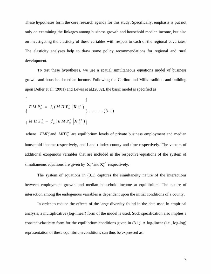
These hypotheses form the core research agenda for this study. Specifically, emphasis is put not

only on examining the linkages among business growth and household median income, but also

on investigating the elasticity of these variables with respect to each of the regional covariates.

The elasticity analyses help to draw some policy recommendations for regional and rural

development.

To test these hypotheses, we use a spatial simultaneous equations model of business

growth and household median income. Following the Carlino and Mills tradition and building

upon Deller et al. (2001) and Lewis et al.(2002), the basic model is specified as

1

2

( ). . . . . . . . . . ( 3 .1)

( )

e mi t i t i t

m hi t i t i t

E M P f M H Y

M H Y f E M P

∗ ∗

∗ ∗

⎧ ⎫⎪ ⎪

=⎪ ⎪⎨ ⎬⎪ ⎪⎪ ⎪= ⎭⎩

X

X

where itEMP∗and itMHY ∗ are equilibrium levels of private business employment and median

household income respectively, and i and t index county and time respectively. The vectors of

additional exogenous variables that are included in the respective equations of the system of

simultaneous equations are given by emitX and mh

itX respectively.

The system of equations in (3.1) captures the simultaneity nature of the interactions

between employment growth and median household income at equilibrium. The nature of

interaction among the endogenous variables is dependent upon the initial conditions of a county.

In order to reduce the effects of the large diversity found in the data used in empirical

analysis, a multiplicative (log-linear) form of the model is used. Such specification also implies a

constant-elasticity form for the equilibrium conditions given in (3.1). A log-linear (i.e., log-log)

representation of these equilibrium conditions can thus be expressed as:

8

( ) ( ) ( ) ( ) ( )

( ) ( ) ( ) ( ) ( )

1 111 1

2 1 1

11

2 122 2

2 1 1

12

1 133

2 133

ln ln ln X (3.2a)

X ln ln ln X (3.2b)

k

k

K Kxd em emit it k it it it k k it

kk

K Kxc mh mhitit it k it it it k k it

kk

EMP MHY EMP d MHY x

MHY EMP MHY c EMP x

∗ ∗ ∗ ∗

==

∗ ∗ ∗ ∗

==

= × → = +

= × → = +

∑∏

∑∏

X

where 2 1 c and d are the exponents on the endogenous variables, for , 1, 2jikx i j = are vectors of

exponents on the exogenous variables, ∏ is the product operator, and for 1, 2iK i = are the

number of exogenous variables in the employment growth and median household income

equations respectively. The log-linear specification has an advantage of yielding a log-linear

reduced form for estimation, where the estimated coefficients represent elasticities. Duffy-Deno

(1998) and MacKinnon, White, and Davidson, 1983) also show that, compared to a linear

specification, a log-linear specification is more appropriate for models involving population and

employment densities.

The literature (Edmiston, 2004; Hamalainen and Bockerman, 2004; Aronsson, Lundberg,

and Wikstrom, 2001; Deller et al., 2001; Henry et al., 1999; Duffy-Deno, 1998; Barkley et al.,

1998; Henry et al., 1997; Boarnet, 1994; Duffy, 1994, Carlino and Mills, 1987; Mills and Price,

1984) suggests that employment and median household income likely adjust to their equilibrium

levels with a substantial lags (i.e., initial conditions). Following the literature a distributed lag

adjustment is introduced and the corresponding partial-adjustment process for each of the

equations given in (3.1) is of the form:

1 1

em

it it

it it

EMP EMPEMP EMP

η∗

− −

⎛ ⎞= ⎜ ⎟⎝ ⎠

( ) ( ) ( ) ( )1 1ln ln lnit it em it em itEMP EMP EMP EMPη η∗− −→ − = − (3.3a)

1 1

mh

it it

it it

MHY MHYMHY MHY

η∗

− −

⎛ ⎞= ⎜ ⎟⎝ ⎠

( ) ( ) ( ) ( )1 1ln ln ln lnit it mh it mh itMHY MHY MHY MHYη η∗− −→ − = − (3.3b)

9

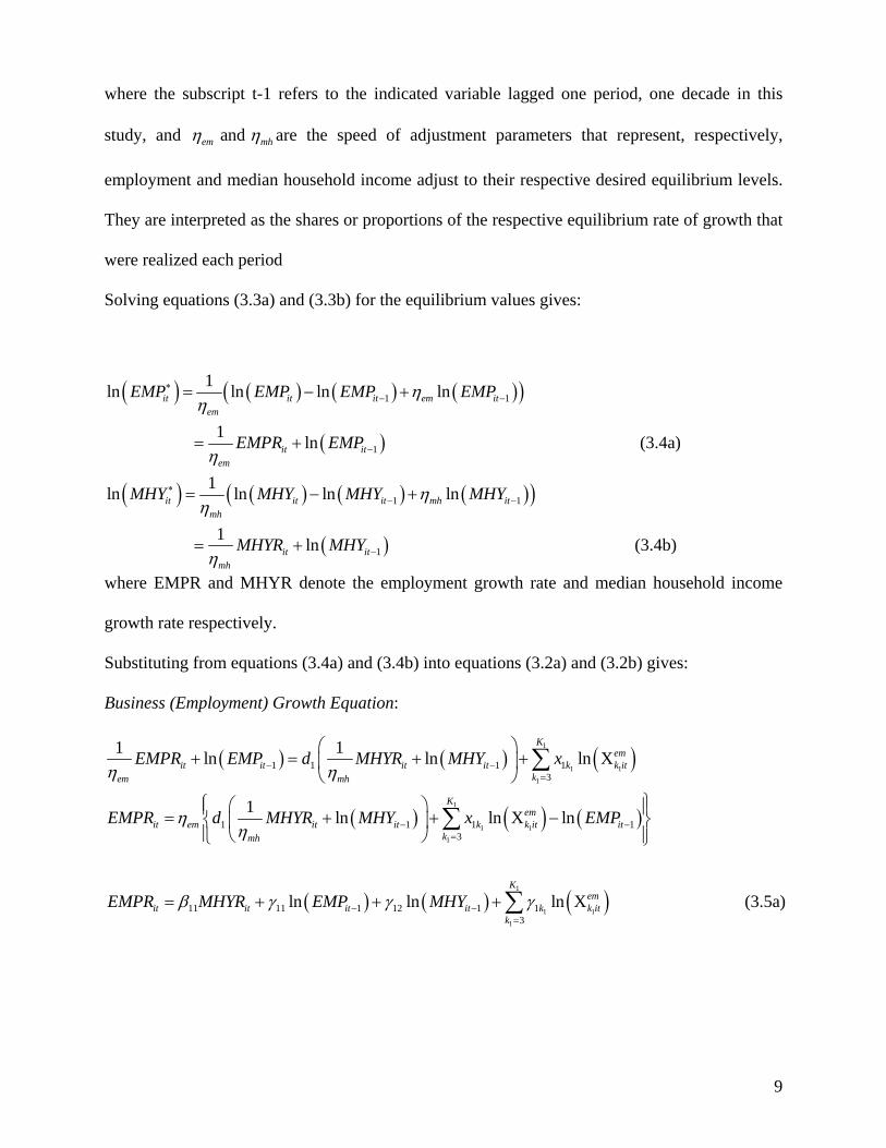
where the subscript t-1 refers to the indicated variable lagged one period, one decade in this

study, and and em mhη η are the speed of adjustment parameters that represent, respectively,

employment and median household income adjust to their respective desired equilibrium levels.

They are interpreted as the shares or proportions of the respective equilibrium rate of growth that

were realized each period

Solving equations (3.3a) and (3.3b) for the equilibrium values gives:

( ) ( ) ( ) ( )( )

( )

1 1

1

1ln ln ln ln

1 ln (3.4a)

it it it em item

it item

EMP EMP EMP EMP

EMPR EMP

ηη

η

∗− −

−

= − +

= +

( ) ( ) ( ) ( )( )

( )

1 1

1

1ln ln ln ln

1 ln (3.4b)

it it it mh itmh

it itmh

MHY MHY MHY MHY

MHYR MHY

ηη

η

∗− −

−

= − +

= +

where EMPR and MHYR denote the employment growth rate and median household income

growth rate respectively.

Substituting from equations (3.4a) and (3.4b) into equations (3.2a) and (3.2b) gives:

Business (Employment) Growth Equation:

( ) ( ) ( )

( ) ( ) ( )

( ) ( )

1

1 1

1

1

1 1

1

1

1 1 1 13

1 1 1 13

11 11 1 12 1 1

1 1ln ln ln X

1 ln ln X ln

ln ln l

Kem

it it it it k k itkem mh

Kem

it em it it k k it itkmh

it it it it k

EMPR EMP d MHYR MHY x

EMPR d MHYR MHY x EMP

EMPR MHYR EMP MHY

η η

ηη

β γ γ γ

− −=

− −=

− −

⎛ ⎞+ = + +⎜ ⎟

⎝ ⎠⎫⎧ ⎛ ⎞⎪ ⎪= + + −⎨ ⎬⎜ ⎟

⎪ ⎝ ⎠ ⎪⎩ ⎭

= + + +

∑

∑

( )1

1

1 3n X (3.5a)

Kemk it

k =∑

10

Median Household Income Growth Equation:

( ) ( ) ( )

( ) ( ) ( )

( ) ( )

2

2 2

2

2

2 2

2

2

1 2 1 23

2 1 2 13

21 21 1 22 1 2

1 1ln ln ln X

1 ln ln X ln

ln ln

Kmh

it it it it k k itkmh em

Kmh

it mh it it k k it itkem

it it it it k

MHYR MHY c EMPR EMP x

MHYR c EMPR EMP x MHY

MHYR EMPR EMP MHY

η η

ηη

β γ γ γ

− −=

− −=

− −

⎛ ⎞+ = + +⎜ ⎟

⎝ ⎠⎧ ⎫⎛ ⎞⎪ ⎪= + + −⎨ ⎬⎜ ⎟

⎪⎪ ⎝ ⎠ ⎭⎩

= + + +

∑

∑

( )2

2

2 3

ln X (3.5b) K

mhk it

k =∑

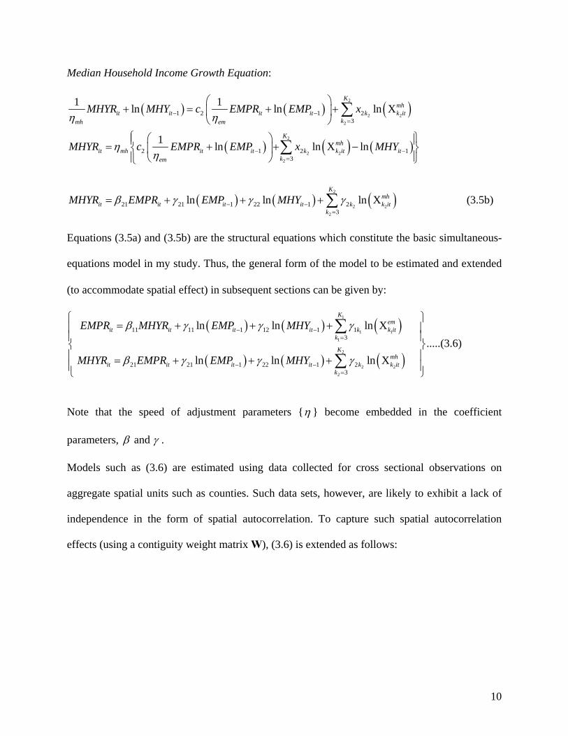
Equations (3.5a) and (3.5b) are the structural equations which constitute the basic simultaneous-

equations model in my study. Thus, the general form of the model to be estimated and extended

(to accommodate spatial effect) in subsequent sections can be given by:

( ) ( ) ( )

( ) ( ) ( )

1

1 1

1

2

2 2

2

11 11 1 12 1 13

21 21 1 22 1 23

ln ln ln X .....(3.6)

ln ln ln X

Kem

it it it it k k itk

Kmh

it it it it k k itk

EMPR MHYR EMP MHY

MHYR EMPR EMP MHY

β γ γ γ

β γ γ γ

− −=

− −=

⎧ ⎫= + + +⎪ ⎪

⎪ ⎪⎨ ⎬⎪ ⎪= + + +⎪ ⎪⎩ ⎭

∑

∑

Note that the speed of adjustment parameters {η } become embedded in the coefficient

parameters, and β γ .

Models such as (3.6) are estimated using data collected for cross sectional observations on

aggregate spatial units such as counties. Such data sets, however, are likely to exhibit a lack of

independence in the form of spatial autocorrelation. To capture such spatial autocorrelation

effects (using a contiguity weight matrix W), (3.6) is extended as follows:

11

( ) ( ) ( )

( ) ( )( ) ( ) ( )

1

1 1

1

11 11 12 11 1

12 1 1 13

21 21 22 21 1

ln

ln ln X +u , where u = u +

ln

it it it it it

Kem em em em em

it k k it it it it itk

it it it it it

EMPR MHYR EMPR MHYR EMP

MHY

MHYR EMPR EMPR MHYR EMP

β λ λ γ

γ γ ρ ε

β λ λ γ

−

−=

−

= + + +

+ +

= + + +

∑

W W

W

W W

( ) ( )2

2 2

2

22 1 2 23

.....(3.7)

ln ln X +u , where u = u + K

mh mh mh mh mhit k k it it it it it

k

MHYγ γ ρ ε−=

⎧ ⎫⎪ ⎪⎪ ⎪⎪ ⎪⎪ ⎪⎨ ⎬⎪ ⎪⎪ ⎪⎪ ⎪+ +⎪ ⎪⎩ ⎭

∑ W

where β, γ, , and λ ρ are unobserved parameters emitu and mh

itu are vectors of disturbances, and

and em mhit itε ε are vectors of innovations. jK , 1, 2j = represents the number of exogenous variables

included in the jth equation. The system in (3.7) is a spatial autoregressive model in which both

the spatial lags in the dependent variables and spatial autoregressive error terms are incorporated.

4. Data The data for the empirical analysis are for the 417 Appalachian counties, which have been

collected and compiled from County Business Patterns, Bureau of Economic Analysis, Bureau of

Labor Statistics, Current Population Survey Reports, County and City Data Book, U.S. Census of

Population and Housing, U.S. Small Business Administration, and Department of Employment

Security. Data for county employment and county median household income are collected for

1990 and 2000. The dependent variables of the model, employment growth rate (EMPR) and

median household growth rate (MHYR), are computed by taking the log difference of the

respective 2000 and the 1990 levels. In addition, data for a number of control variables are

collected for 1990 from the different sources (see table 1 for the data description).

Table 1 about here 5. Estimation Issues and Results

The model given in (3.7) is estimated using generalized spatial two stage least squares

(GS2SLS) and generalized spatial three stage least squares (GS3SLS) procedures. This is done,

12

respectively, in a three and a four step routines. The first three steps are common for both. In the

first step, the parameter vector consisting of betas, lambdas and gammas [ ], ,β λ γ′ ′ ′ are estimated

by two stage least squares (2SLS) using an instrument matrix that consists of 2X, WX, W X ,

where X is the matrix that includes all control variables in the model, and W is a weight matrix.

The disturbances for each equation in the model are computed by using the estimates for betas,

lambdas and gammas from the first step. In the second step, these estimates of the disturbances

are used to estimate the autoregressive parameter rho ( )ρ for each equation using Kelejian and

Prucha’s generalized moments procedure. In the third step, a Cochran-Orcutt-type transformation

is done by using the estimates for rhos from the second step to account for the spatial

autocorrelation in the disturbances. The GS2SLS estimators for betas, lambdas and gammas are

then obtained by estimating the transformed model using ⎡ ⎤⎣ ⎦2X, WX, W X as the instrument

matrix.

Although the GS2SLS takes the potential spatial correlation in to account, it does not

utilize the information available across equation because it does not take into account the

potential cross equation correlation in the innovation vectors ( ),em mhit itε ε . The full system

information is utilized by stacking the Cochran-Orcutt-type transformed equations (from the

second step) in order to estimate them jointly. Thus, in the fourth step the GS3SLS estimator of

betas, lambdas, and gammas is obtained by estimating this stacked model. The GS3SLS

estimator is more efficient relative to GS2SLS estimator.

Table 2 about here

The GS2SLS and GS3SLS parameter estimates of the system given in (3.7) for the 1990-

2000 is presented in Table 2. A detailed discussion of the performance of each control variable is

not pursued due to space limitation. But, some highlights of the analysis warrants discussion. Let

13

us first see the results for the employment equation (EMPR). These results suggest a positive and

significant parameter estimate for lambda1 that indicate that employment growth rate tends to

spillover to neighboring counties and have a positive effect on their employment growth rates.

The results also show a positive parameter estimate for lambda2 that indicate that median

household income growth rates (MHYR) in neighboring counties tends to affect favorably

EMPR in a given county. These are important from a policy perspective as they indicate that

employment growth and growth in median household incomes in one county are not at the

expense of EMPRs in neighboring counties. The results are also important from an economic

perspective because these significant spatial lag effects indicate that EMPR does not only depend

on characteristics within the county, but also on that of its neighbors. Hence, spatial effects

should be tested for in empirical works involving employment growth rates and household

income growth rates. Our model specification incorporates spatially autoregressive spatial

process (effect) besides the spatial lag in the dependent variables. The results in Table 2 suggest

a negative parameter estimate for rho1 indicating that random shocks into the system with

respect to EMPR do not only affect the county where the shocks originated and its neighbors, but

create negative shock waves across Appalachia.

The elasticity of EMPR with respect to the initial employment level (EMP90) is negative

and statistically significant indicating convergence in the sense that counties with initial low

level of employment at the beginning of the period (1990) tend to show higher rate of growth of

business than counties with high initial level of employment conditional on the other explanatory

variables in the model. This result supports prior results of rural renaissance in the literature

(Deller et al, 2001; Lunderberg, 2003).

To control for agglomeration effects, our model includes initial county population size

(POPs) and population density (POPd). As expected, the results show that POPs have positive

and significant effects on EMPR. However, although it has the proper sign, POPd is not

14

significant. In contradiction to the theoretical expectations, the results show initial human capital

endowment as measured by the percentage of adults (over 23 years old) with college degree and

above (POPCD) has the wrong sign. One interpretation of this result is that the jobs created in

Appalachia during the study period were, on average low paying jobs which do not require high

human capital. This interpretation may be corroborated by positive coefficient on POPHD (the

percentage of adults (over 23 years old) with high school diploma or higher). We also include

county unemployment rate (UNE) in our vector of exogenous variables as a measure of local

economic distress. Our results suggest that high unemployment rate is associated with low

business growth. This indicates that the poor economic environment in Appalachia did not

provide incentive for individuals to form new business that can employ not only the owner, but

others.

Establishment density (ESBd), which is the total number of private sector establishments in the

county divided by the total county’s population, is included in our model to capture the degree of

competition among firms and crowding of businesses relative to the population. The average

size of establishment (ESBs), defined as the total private sector employment divided by the total

number of private establishments in the county, is also included to capture the effects of barriers

to entry of new small firms on employment growth. The coefficient on ESBD is positive and

significant indicating that Appalachia region is far below the threshold where competition among

firms for consumer demands crowds businesses. According to our results, High ESBd is

associated with growth in Employment (business growth), indicating that firms tend to locate

near each other possibly due to localization and agglomeration economies of scale. The

coefficient on ESBs is also positive and significant indicating existence of low barrier to new

firm formation and employment generation in Appalachia during the study period.

One interesting observation from our results pertains to the role of local government on

business growth. Our model predicts that local governments, through their spending and taxation

15

functions, have critical roles in creating enabling economic environments for businesses to

prosper. The results of our model, however, predict that local governments had not played

significant roles in employment growth in Appalachia. Given the economic hardship and high

level of underdevelopment in Appalachia, these results are indications that local governments

should step up their efforts to create incentives in order to encourage business growth in the

region.

Now let us turn to the results of the MHYR equation. Unlike the results of the EMPR

equation, these results suggest a negative parameter estimate for lambda2 that indicates that

MHYR tends to spillover to neighboring counties and have a negative effect on their

employment growth rates,, although insignificant. . The results also show a negative parameter

estimate for lambda1 that indicate that EMPR in neighboring counties tends to affect

unfavorably MHYR in a given county. These are important from a policy perspective as they

indicate that employment growth and growth in median household incomes in one county are at

the expense of MHYRs in neighboring counties.

The results also indicate a positive parameter estimate for rho2 indicating that random

shocks into the system with respect to MHYR do not only affect the county where the shocks

originated and its neighbors, but create positive shock waves across Appalachia. The elasticity of

EMPR with respect to the initial median household income (MHY90) is negative and statistically

significant indicating convergence in the sense that counties with initial low level of median

household income at the beginning of the period (1990) tend to show higher rate of growth of

median household income than counties with high initial level of median household income

conditional on the other explanatory variables in the model.

The coefficient on the index of social capital (SCIX) is positive and significant indicating

counties with high level of social capital increase the wellbeing of their communities. The

coefficients on the proportion of population of school age (POP5-17), the proportion of

16

population above 65 years old (POP>65), on the proportion of female headed households

(FHHF) indicate the expected signs, negative, positive and negative respectively. Counties with

higher proportions of POP5-17 and FHHF tend to have lower level of median household income.

Whereas, counties with higher proportion of POP>65 tend to have higher levels of MHY. These

results are in line with the results in the literature.

The coefficients on beta1 and beta2 are positive indicating positive relationships between

EMPR and MHYR. EMPR affects MHYR and MHYR affects EMPR but the strength of effects

are different with the effect of EMPR on MHYR stronger (0.2825>0.1685).

5. Conclusions

The main issue in this paper has been to test the hypotheses that (1) business growth and median

household income are interdependent and are jointly determined by regional covariates; (2)

growth is conditional upon initial conditions; and (3) growth in county is conditional upon

growth in neighboring counties. To test these hypotheses, we developed a spatial simultaneous

equations model. GS2SLS and GS3SLS estimators are obtained by estimating the model using

data covering the 417 Appalachian counties for the 1990-2000. We find evidences in support of

all the three hypotheses. In particular, we find that EMPR in one county is positively affected by

EMPR and MHYR in neighboring counties, whereas, MHYR in one county is negatively

affected by EMPR and MHYR in neighboring counties. Our results also indicate the presence of

spatial correlation in the error terms. This implies that a random shock into the system spreads

across the region. The policy implications of the existence of these spatial spillover and spatial

autoregressive effects is that there should be a regional approach to promoting business growth

and income creation in Appalachia. The results also indicate convergence across counties in

Appalachia with respect to EMPR and MHYR conditional upon the initial conditions of the

explanatory variables in the model

17

Table 1: Descriptive statistics for year 1990

Variable Code Variable Description Mean Std Dev Minimum Maximum

Constant 1.00 0.00 1.00 1.00 EMPR Employment growth rate 1990-2000 0.17 0.25 -0.69 1.79 MHYR Median Household income growth rate 1990-2000 0.48 0.31 -0.49 1.40 WEMPR Spatial Lag of EMPR 0.18 0.14 -0.18 0.81 WMHYR Spatial lag of MHYR 0.47 0.19 -0.11 1.02 POPs Population 1990 10.30 0.94 7.88 14.11 POPd Population density 1990 4.28 0.90 1.85 7.75 POP5-17 Percent of population between 5 -17 years 1990 2.92 0.12 2.17 3.22 POP25-44 Percent of population between 25 -14 years old 1990 3.38 0.08 2.79 3.74 POP>65 Percent of population above 65 years old 1990 2.60 0.20 1.55 3.20 FHHF percent of female householder, family householder, 1990 2.32 0.20 1.81 3.19 POPHD Persons 25 years and over, % high school or higher, 1990 4.10 0.17 3.57 4.47 POPCD Persons 25 years and over, % Bachelor's degree or above, 1990 2.27 0.41 1.31 3.73 OWHU Owner-Occupied Housing Unit in percent, 1990 4.33 0.08 3.87 4.47 MHU Median Value of owner occupied housing 1990 10.74 0.26 9.67 11.68 UNEMP Unemployment rate 1990 2.15 0.35 1.22 3.25 AGFF % employed in Agr., forestry and fisheries 1990 3.62 2.66 0.00 17.10 MANU % employed in manufacturing 1990 3.14 0.57 0.79 3.98 WHRT % employed in wholesale and retail trade 1990 2.92 0.19 2.16 3.32 FIRE % employed Finance, Insurance and Real Estate 1990 1.23 0.33 0.00 2.23 HLTH % employed Health service 1990 1.95 0.34 0.74 3.44 NAIX Natural Amenities Index 1990 0.14 1.16 -3.72 3.55 ESBD Establishment density 1990 2.93 0.34 1.87 4.09 EFIR Earnings in Finance Insurance and real Estate 1990 21075.08 96011.09 0.00 1638807.0CSBD Commercial and Saving Banks deposits 1990 12.21 1.07 8.83 16.95 DFEG Direct federal expenditure and grants per capita 1990 7.99 0.38 6.98 10.18 FGCE Federal gover't civilian employment per 10,000 pop. 1990 60.48 101.03 0.00 1295.00 PCTAX Per capital local tax 1990 5.91 0.53 4.51 7.42 PCPTAX Property tax per capita 1990 5.52 0.62 3.91 7.36 SCIX Social Capital Index 1987 -0.60 0.94 -2.53 5.64 HWD Highway Density 1990 0.69 0.40 -0.34 2.63 ESBs Establishment size 1990 2.53 0.30 1.49 3.60 AWSR Average annual wage and salary rate 1990 9.75 0.19 9.31 10.35 EMP Employment 1990 8.83 1.25 5.42 13.38 INMG In-migration 1990 7.09 1.00 4.54 10.52 OTMG out-migration 1990 7.04 0.97 4.50 10.55 MHY Median Household income 1989 9.94 0.23 9.06 10.68 DGEX Direct general exp. Per capita 1992 7.23 0.28 6.49 8.11

Note: All the variables are expressed in log terms except AGFF, EFIR, FGCE, SCIX, and NAIX

18

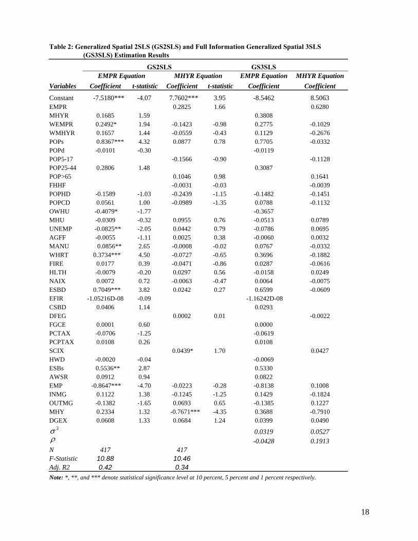
Table 2: Generalized Spatial 2SLS (GS2SLS) and Full Information Generalized Spatial 3SLS (GS3SLS) Estimation Results

GS2SLS GS3SLS EMPR Equation MHYR Equation EMPR Equation MHYR Equation Variables Coefficient t-statistic Coefficient t-statistic Coefficient Coefficient

Constant -7.5180*** -4.07 7.7602*** 3.95 -8.5462 8.5063 EMPR 0.2825 1.66 0.6280 MHYR 0.1685 1.59 0.3808 WEMPR 0.2492* 1.94 -0.1423 -0.98 0.2775 -0.1029 WMHYR 0.1657 1.44 -0.0559 -0.43 0.1129 -0.2676 POPs 0.8367*** 4.32 0.0877 0.78 0.7705 -0.0332 POPd -0.0101 -0.30 -0.0119 POP5-17 -0.1566 -0.90 -0.1128 POP25-44 0.2806 1.48 0.3087 POP>65 0.1046 0.98 0.1641 FHHF -0.0031 -0.03 -0.0039 POPHD -0.1589 -1.03 -0.2439 -1.15 -0.1482 -0.1451 POPCD 0.0561 1.00 -0.0989 -1.35 0.0788 -0.1132 OWHU -0.4079* -1.77 -0.3657 MHU -0.0309 -0.32 0.0955 0.76 -0.0513 0.0789 UNEMP -0.0825** -2.05 0.0442 0.79 -0.0786 0.0695 AGFF -0.0055 -1.11 0.0025 0.38 -0.0060 0.0032 MANU 0.0856** 2.65 -0.0008 -0.02 0.0767 -0.0332 WHRT 0.3734*** 4.50 -0.0727 -0.65 0.3696 -0.1882 FIRE 0.0177 0.39 -0.0471 -0.86 0.0287 -0.0616 HLTH -0.0079 -0.20 0.0297 0.56 -0.0158 0.0249 NAIX 0.0072 0.72 -0.0063 -0.47 0.0064 -0.0075 ESBD 0.7049*** 3.82 0.0242 0.27 0.6599 -0.0609 EFIR -1.05216D-08 -0.09 -1.16242D-08 CSBD 0.0406 1.14 0.0293 DFEG 0.0002 0.01 -0.0022 FGCE 0.0001 0.60 0.0000 PCTAX -0.0706 -1.25 -0.0619 PCPTAX 0.0108 0.26 0.0108 SCIX 0.0439* 1.70 0.0427 HWD -0.0020 -0.04 -0.0069 ESBs 0.5536** 2.87 0.5330 AWSR 0.0912 0.94 0.0822 EMP -0.8647*** -4.70 -0.0223 -0.28 -0.8138 0.1008 INMG 0.1122 1.38 -0.1245 -1.25 0.1429 -0.1824 OUTMG -0.1382 -1.65 0.0693 0.65 -0.1385 0.1227 MHY 0.2334 1.32 -0.7671*** -4.35 0.3688 -0.7910 DGEX 0.0608 1.33 0.0684 1.24 0.0399 0.0490

2σ 0.0319 0.0527 ρ -0.0428 0.1913 N 417 417 F-Statistic 10.88 10.46 Adj. R2 0.42 0.34 Note: *, **, and *** denote statistical significance level at 10 percent, 5 percent and 1 percent respectively.

19

References Acs, Z. J. and C. Armington, 2004, “The Impact of Geographic Differences in Human Capital

on Service Firm Formation Rates,” Journal of Urban Economics, forthcoming. _______, 2002. “Endogenous Growth and Entrepreneurial Activity in Cities,” Regional Studies,

forthcoming. Acs, Z. J. and D. B. Audretsch, 2001, “The Emergence of the Entrepreneurial Society”,

Presentation for the Acceptance of the 2001 International Award for Entrepreneurship and Small Business Research, 3 May, Stockholm.

Aronsson, T., J. Lundberg and M. Wikstrom, 2001, “Regional Income Growth and Net Migration in Sweden 1970-1995,” Regional Studies, forthcoming.

Audretsch D. B. and M. Fritsch, 1994, “The Geography of Firm Births in Germany,” Regional Studies 28(4): 359-365.

Audretsch, D.B., M.A. Carree, A.J. van Stel and A.R. Thurik, 2000, Impeded Industrial Restructuring: The Growth Penality, Research Paper, Center for Advanced Small Business Economics, Erasmus University, Rotterdam, Netherlands.

Barkley, D.L., M.S. Henry, and S. Bao, (1998), “The Role of Local School Quality and Rural Employment and Population Growth”, Review of regional Studies, 28 (summer): 81-102.

Boarnet, M.G., (1994), “An Empirical Model of Intra-metropolitan Population and Employment Growth,” Papers in Regional Science, 73 (April): 135-153.

Callejon, M. and A. Segarra, 2001, “ Geographical Determinants of The Creation of Manufacturing Firms: The Regions of Spain,” http://www.ub.es/graap/callejon.htm

Carlino, O.G. and E.S. Mills, 1987, “The Determinants of County Growth,” Journal of Regional Science 27(1): 39-54.

Christensen, G., 2000, “Entrepreneurship Education: Involving Youth in Community Development,” Nebraska Department of Education, Marketing and Entrepreneurship Education, Lincoln, NE.

Clark, D. and C.A. Murphy, 1996, “Countywide Employment and Population Growth: An Analysis of the 1980s,” Journal of Regional Science 36(2): 235-256.

Cushing, Brain, and Cyntia Rogers, 1996, “Income and Poverty in Appalachia,” Socio-Economic Review of Appalachia( Papers Commissioned by the Appalachia Regional Commission), Regional Research Institute, West Virginia University.

Davidson, P., L. Lindmark and C. Olofsson, 1994, “New Firm Formation and Regional Development in Sweden,” Regional Studies 28: 395-410.

Deavers, Kenneth L., and Robert A. Hoppe, 1992, “Overview of the Rural Poor in the 1980s,” in Cynthia Duncan (ed.), Rural Poverty in America, Westport CT: Greenwood Publishing Group Inc.

Deller, Steven C., Tsung-Hsiu Tsai, David W. Marcouiller, and Donald B.K. English, (2001), “The Role of Amenities and Quality of Life in Rural Economic Growth,” Journal of American Agricultural Economics, 83(3): 352-365.

Dilger, Robert Jay, and Tom Stuart Witt, 1994, “West Virginia’s Economic Future, “ in Dilger Robert Jay and Tom Stuart Witt (eds.), West Virginia in the 1990s: Opportunities for Economic Progress, Morgantown: West Virginia University Press.

Duffy, N.E., (1994), “The Determinants of State Manufacturing Growth Rates: A Two-Digit-Level Analysis,” Journal of Regional Science, 34(May): 137-162.

20

Duffy-Deno, K.T., (1998), “The Effect of Federal Wilderness on County Growth in the Inter-mountain Western United States,” Journal of Regional Sciences, 38(February): 109-136.

Duffy-Deno, Kevin T. and Randall W. Eberts, 1991, “Public Infrastructure and Regional Economic Development: A Simultaneous Equations Approach,” Journal of Urban Economics 39: 329-343.

Edmiston, Kelly D., (2004), “The Net Effect of Large Plant Locations and Expansions on Country Employment,” Journal of Regional Science, 44(2): 289-319.

Ekstrom, B., and F. L. Leistritz, 1988, Rural community decline and revitalization: An annotated Bibliography. New York: Garland Publishing. Inc.,

Evans, D. and L. S. Leighton, 1990, “Small Business Formation By Unemployed and Employed Workers,” Small Business Economics 2:319-330.

Fisher, Ronald, 1997, “ The effects of State and Local Public Services on Economic Development,” New England Economic Review, March/April: 53-67.

Fotopoulos, G. and N. Spencer, 1999, “Spatial Variations in New Manufacturing Plant Openings: Some Empirical Evidence from Greece,” Regional Studies, 33(3): 219-229.

Fritsch, M., 1992, “Regional Differences in New Firm Formation: Evidence from West Germany,” Regional Studies 26:233-244.

Fritsch, M. and O. Falck, 2003, “New Firm Formation by Industry over Space and Time: A Multilevel Analysis,” Discussion Paper, German Institute for Economic Research, Berlin.

Gabe, Todd M. and Kathleen P. Bell, 2004,“Tradeoff Between Local Taxes and Government Spending as Determinants of Business Location,” Journal of Regional Science 44(1): 21-41.

Garofoli, G., 1994, “New Firm Formation and Regional Development: The Italian Case,” Regional Studies 28:381-393.

Greenwood, M. J. and G.L. Hunt, 1984 “ Migration and Interregional Employment Redistribution in the United States,” American Economic Review 74(5): 957-969.

Greenwood, M.J. et al., 1986, “Migration and Employment Change: Empirical Evidence on Spatial and Temporal Dimensions of The linkage,” Journal of Regional Science 26(2): 223-234.

Glaeser, E.L., J.A. Scheinkman and A. Shleifer, 1995, “Economic Growth in a Cross-Section of Cities,” Journal of Monetary Economics 36(1): 117-143.

Guesnier, B, 1994, “Regional Variation in New Firm Formation in France,” Regional Studies 28(4): 347-358.

Hamalainen, Kari, and Petri Bockerman, (2004), “Regional Labor Market Dynamics, Housing, and Migration,” Journal of Regional Science, 44(3): 543-568.

Hart, M. and G. Gudgin, 1994, “ Spatial Variations in New Firm Formation in the Republic of Ireland, 1980-1990,” Regional Studies 28(4): 367-380.

Hayness, Ada F., 1997, Poverty in Central Appalachia: Underdevelopment and Explotiation, New York: Garland Publishing, Inc.

Henry, M.S., D.L. Barkley, and S. Bao, (1997), “The Hinterland’s Stake in Metropolitan Growth: Evidence from Selected Southern Regions,” Journal of Regional Science, 37(August): 479-501.

Henry, M.S., B. Schmitt, K Kristensen, D.L. Barkley, and S. Bao, (1999), “Extending Carlino-Mills Models to Examine Urban Size and Growth Impacts on Proximate Rural Areas,” Growth and Change, 30(Summer): 526-548.

Highfield, R. and R. Smiley, 1987, “ New Business Starts and Economic Activity: An Empirical Investigation,” International Journal of Industrial Organization 5.

21

Johnson, P. and S. Parker, 1996, “ Spatial Variations in the Determinants and Effects of Firm Births and Deaths,” Regional Studies 30(7): 676-688.

Kangasharju, A., 2000, “Regional Variations in Firm Formation: Panel and Cross-Section Data Evidence from Finland,” Regional Science 79:355-373.

Keeble, D. and S. Walker, 1994, “ New Firms, Small Firms and Dead Firms: Spatial Pattern and Determinants in the United Kingdom,” Regional Studies 28(4): 411-427.

Kelejian, Harry H., and Ingram R. Prucha, (2004), “Estimation of Simultaneous Systems of Spatially Interrelated Cross Sectional Equations,” Journal of Econometrics, 118:27-50.

Lewis, David J., Gray L. Hunt and Andrew J. Plantigna, 2002, “ Does Public Land Policy Affect Local Wage Growth,” Growth and Change 34(1): 64-86.

Lundberg, J. 2003, “On the Determinants of Average Income Growth and Net Migration at the Municipal Level in Sweden,” Review of Regional Studies, forthcoming.

MacDonald, John F., 1992, “ Assessing the Development Status of Metropolitan Areas,” in Edwin S.Mills and John F. MacDonald (ed.), Sources of Metropolitan Growth, New Brunswick, NJ: Center for Urban Policy Research.

Mackinnon, J.G., H. White, and R. Davidson, (1983), “Tests for Model Specification in the Presence of Alternative Hypotheses: Some Further Results,” Journal of Econometrics, 21: 53-70.

Maggar, Sally W., 1990, “ Schooling, Work Experience and Gender: The Social Reproduction of Poverty in Mining Regions,” Research Paper 9014, Regional Research Institute, Morgantown: West Virginia University Press.

Mills, E.S., and R. Price, (1984), “Metropolitan Suburbanization and central City Problems,” Journal Urban Economics, 15: 1-17.

Persson, J., 1997, “ Convergence Across the Swedish Counties, 1911-1993,” European Economic Review 41: 1834-1852.

Pulver, G. C., 1989, “Developing a community perspective on rural economic development policy.” Journal of Community Development Society 20: 1-4.

Reynolds, P.D., 1994, “ Autonomous Firm Dynamics and Economic Growth in the United States, 1986-1990,” Regional Studies 28(4): 429-442.

______, 1999, “Creative Distruction,” in Acs, et al.,(eds.), Entrepreneurship, Small and Medium-Sized Enterprises and the Macroeconmy, Cambridge University Press: Cambridge, U.K.

Rupasingha, A. and S.J. Goetz, 2003, “ County Ammenties and Net Migration,” Paper Presented in WRSA Annual Meeting, Rio Rico, Arizona, Feb 26-March 1, 2003.

Steinnes, Donald N. and Walter D. Fisher, 1974, “An Econometric Model of Intraurban Location,” Journal of Regional Science 14: 65-80.

Thurik, A. R. and S. Wennekers, 1999, “Linking Entrepreneurship and Economic Growth,” Small Business Economics 13(1): 27-55.