Journal of Magnetic Resonance 207 (2010) 59–68

Contents lists available at ScienceDirect

Journal of Magnetic Resonance

journal homepage: www.elsevier .com/locate / jmr

An electromagnetic reverse method of coil sensitivity mapping for parallel MRI– Theoretical framework

Jin Jin a, Feng Liu a, Ewald Weber a, Yu Li a, Stuart Crozier b,⇑a MedTeQ Centre, The School of Information Technology and Electrical Engineering, The University of Queensland St. Lucia, Brisbane, Qld 4072, Australiab Biomedical Engineering Director, MedTeQ Centre, The School of Information Technology and Electrical Engineering, The University of Queensland, St. Lucia, Brisbane,Qld 4072, Australia

a r t i c l e i n f o a b s t r a c t

Article history:Received 17 March 2010Revised 2 August 2010Available online 17 August 2010

Keywords:Parallel imagingSensitivityMappingReconstruction

1090-7807/$ - see front matter Crown Copyright � 2doi:10.1016/j.jmr.2010.08.009

⇑ Corresponding author. Fax: +61 (0)7 3365 4999.E-mail addresses: jinjin@itee.uq.edu.au (J. Jin),

ewald@itee.uq.edu.au (E. Weber), yuli@itee.uq.edu.au(S. Crozier).

In this paper, a novel sensitivity mapping method is proposed for the image domain parallel MRI (pMRI)technique. Instead of refining raw sensitivity maps by means of conventional image processing opera-tions such as polynomial fitting, the presented method determines coil sensitivity profiles through aniterative optimization process. During the algorithm implementation the optimization cost function isdefined as the difference between the raw sensitivity profile and the desired profile. The minimizationis governed by the physics of low-frequency electromagnetic and reciprocity theories. The performanceof the method was theoretically investigated and compared with that of a traditional polynomial fitting,against a range of system noise levels. It was found that, the new method produces high-fidelity sensi-tivity profiles with noise amplitudes, measured as root mean square deviation an order of magnitude lessthan that of the polynomial fitting method. Using the sensitivity profiles generated by our method, SENSE(sensitivity encoding) reconstructions produce significantly less image artefacts than conventional meth-ods. The successful implementation of this method has far-reaching implications that accurate sensitivitymapping is not only important for parallel reconstruction, but also essential for its transmission analogy,such as Transmit SENSE.

Crown Copyright � 2010 Published by Elsevier Inc. All rights reserved.

1. Introduction

In this paper, a novel sensitivity mapping method is proposedfor image domain parallel reconstruction algorithms. Instead ofrefining raw sensitivity maps by means of image processing oper-ations or polynomial fitting procedures, the presented methoddetermines the coil sensitivity profiles by resorting to physics ofelectromagnetics.

Parallel imaging (PI) is used widely in advanced MRI applica-tions. Complementing gradient encoding schemes, spatial encod-ing by means of distinct coil sensitivities is incorporated into PIto improve scan speed and coverage [1]. Sensitivity encoding(SENSE) [2,3] and generalized auto calibrating partially parallelacquisitions (GRAPPA) [4] methods continue to be the two mostpopular PI methods. SENSE represents a class of image domainmethods [2,5,6], in which the reconstruction coefficients arecalculated in the image domain, whereas GRAPPA and its variants[4,7–9], known as spatial-frequency domain methods, acquire

010 Published by Elsevier Inc. All r

feng@itee.uq.edu.au (F. Liu),(Y. Li), stuart@itee.uq.edu.au

reconstruction coefficients in K-space. These seemingly distinctclasses of methods can be seen as different approaches to solvingthe same set of linear equations of inverse problems [10]. A distinc-tion between the two approaches is that image domain methodsrequire an explicit extraction of the coil sensitivities, whereas sen-sitivity information is involved in spatial-frequency domain meth-ods implicitly. Despite the extra work of sensitivity mapping,image domain methods are often preferred since they can provideaccurate solutions to the inverse problem and achieve an optimalreconstruction [11] provided the sensitivities are known exactly,whereas GRAPPA gives a solution based on approximating the lin-ear combination coefficients for the repopulation of the missingK-space lines. Furthermore, SENSE can outperform GRAPPA insome imaging scenarios since it allows greater opportunity tocontrol reconstruction quality through regularization [12].Traditionally, the sensitivity profile of a coil is defined by the divi-sion between a coil image and a uniform reference image, whichare obtained from reference scans of a body coil or sum-of-squaresof surface coil arrays [2]. This raw sensitivity profile is then refinedby two-dimensional polynomial fitting [2]. Dynamic self-calibrat-ing methods [13] have been developed to deal with sensitivity mis-registration that can result from the traditional methods. However,the truncation in the spatial-frequency domain of the dynamic

ights reserved.

60 J. Jin et al. / Journal of Magnetic Resonance 207 (2010) 59–68

methods causes Gibbs phenomena. Apodization, wavelet de-nois-ing techniques [14] and polynomial fitting [2,15] have been usedto reduce Gibbs ringing, however, these methods all have difficultycancelling the ringing errors [15].

Here we propose a novel sensitivity mapping method based onthe theory of reciprocity [16,17], which allows the evaluation ofthe receiving sensitivity from transmitting Bþ1 field. In this ap-proach, the measured raw sensitivity profile is first used to inver-sely determine the coil array geometry by solving the associatedelectromagnetic problem. With the coil array information known,the coil sensitivity profile can then be calculated as the B1 recep-tion field (B�1 ). In this proof-of-concept research, we will focus onlow fields (B0 6 1.5T) in the so-called near-field regime, wherethe RF wavelength k is much larger than the object and the coil ar-ray. As the problem is reduced to quasi-static in this regime, the setof four Maxwell’s equations are reduced to Ampere’s Law for thecalculation of magnetic field. As a result, the reciprocal magneticfield (B�1 ) can be calculated by Biot–Savart integration derived fromAmpere’s law with quasi-static limit, since the RF field is weaklydistorted by the object being scanned [1,18,19]. The proposedmethod will be demonstrated in two cases: the sensitivity map-ping for a single coil element and the sensitivity mapping for anelement in a four-element array. A performance comparison ofthe proposed and the traditional polynomial fitting method willbe carried out, for both scenarios.

2. Methods

Similar to our recent work on exposure evaluations by reverse-engineering of gradient coils [20], the geometry of a typical radiofrequency (RF) coil can be inversely determined from the measuredmagnetic field information. In low field cases, this reverse methodis made possible by the reasons that the RF coil can be representedby a mathematical model using a few model descriptors. Then,using the principle of reciprocity [16,17] we are able to reproducethe measured B1 field propagation using Biot–Savart integrationwith steady current flowing in the coil element. With appropriateparameterization, an optimization algorithm can then be used toattain the values of descriptors representing the RF coil geometry.

Firstly, this work will review the traditional sensitivity mappingmethod, which serves as a basis for evaluation and comparison.Using the two sensitivity mapping case studies, we then derive a

Fig. 1. Coil sensitivity mapping procedure proposed by Prussmann et al. An array imagethen masked to obtain a profile with only reliable sensitivity information (D). The extrdimensional local polynomial fit is performed to acquire the sensitivity map (F).

framework for acquiring sensitivity profiles from a raw sensitivitymap and limited information of coil array geometry. Case I willshow, in the simplest way, how a noisy sensitivity profile is de-noised by the new method. In Case II, the method is extended tohandle coil arrays. In these studies, noise is introduced into the sys-tem in a controlled manner.

2.1. Conventional image-domain coil sensitivity mapping

Noise is inevitably found in any MR image and consequently inthe measured sensitivity maps. One of the conventional methodsfor sensitivity mapping and noise mitigation was introduced byPruessmann et al. [2], alongside the SENSE method. The procedureis illustrated in Fig. 1. Here a coil image (A) is divided by a uniformreference image (B) to produce a raw sensitivity map (C). However,noise in the raw sensitivity map, augmented by the division, is usu-ally a serious issue during this procedure, particularly in areas withlow proton density [21], such as the ‘holes’ which appeared inFig. 1C. To mitigate contaminating noise, profile C is masked by abinary profile, which is obtained by applying a threshold on theuniform reference image (B). A profile of sensitivity informationwithin the reliable region (D) is thus obtained. The extrapolationzone (E) is produced by a morphological region-growing approach.A two-dimensional local polynomial fit, based upon the assumptionthat coil sensitivity has a slowly changing profile, is performed onthe extrapolation zone to acquire the refined sensitivity map (F).

2.2. Case I – single coil element

A sensitivity profile is a function of the coil geometry, objectcharacteristics and the resonant frequency. The single coil modelshown in Fig. 2A consists of only one element of a typical RF coilarray and a spherical phantom. The coil element is specified by afew descriptors: c representing the opening of the coil element, arepresenting the azimuth angle with respect to 0� of the cylindricalcoordinate system and �I representing the resonant current. Usingthese parameters, the functional dependence of the magnetic fieldcan be described as:

B0 ¼ F0ðc;a;�IÞ ð1Þ

where the sensitivity profile B0 is a function of parameters c, a,and �I.

(A) is divided by a body coil image (B) to produce a raw sensitivity map (C), which isapolation zone (E) is produced by a morphological region growing approach. Two-

Fig. 2. A. Coil Geometry and Model Descriptors. I represents the resonant current. c is the opening angle of the coil. a is the azimuth angle with respect to x-axis. (a equalszero in current case) The field-of-field (FOV) is located in the centre slice (Z = 0) of the spherical phantom. R is the distance from the centre of FOV to the vertical wires. H is thelength of the vertical wires. (B): The simulated sensitivity profile obtained from FOV. C: The noised-added sensitivity profile, with sampling points representing sensitivitycharacteristics (blue dots). (For interpretation of the references to colour in this figure legend, the reader is referred to the web version of this article.)

J. Jin et al. / Journal of Magnetic Resonance 207 (2010) 59–68 61

Clearly, an accurate description of this functional dependence iscrucial for the proposed method. The field has dependence on coilarray geometry, specified by c and a, current �I of the coil, as well asthe resonance frequency of the MR system. At low fields, the quasi-static magnetic approximation applies. A set of four Maxwell’sEquations are reduced to Ampere’s Law with steady current forthe calculation of magnetic field strength using Eq. (1). By virtueof the principle of reciprocity [16,17], the sensitivity profile canbe obtained from the (hypothetical) RF field as long as the functionF 0 can successfully describe the dependence of B0 on the parame-ters. An optimization process can be utilized to determine a set ofparameter values that generate the least square fit to the measuredprofile. A general form of the optimization cost function that quan-tifies the discrepancy between the hypothetical and the measuredfield is:

U ¼ ðB0 � B0Þ � ðB0 � B0ÞH ð2Þ

where B0 is the hypothetical field with dependence on c, a, �Ithrough function F0; and B0 is the measured sensitivity profile;and the superscript H denotes conjugate transpose.

Case I is a simplified scenario, which shows how a noisy sensi-tivity profile is de-noised by the new method. A scheme was de-signed to incorporate the noise into the system in a quantitativemanner. Firstly, a noise-free sensitivity profile (Fig. 2B) was calcu-lated by employing electromagnetic simulation software FEKO(EMSS, SA). The coil element was numerically tuned to resonateat 64 MHz and the magnetic field in X–Y plane was studied atZ = 0. Granted by the principle of reciprocity [16], the coil sensitiv-ity profile (B�1 ) was readily available once the Bþ1 field was obtained.In this study, the model parameters are as follows: phantom rela-tive permeability er = 30, conductivity r1 = 0.3S/m, mass densityq1 = 1030 kg/m3, coil height h = 90 mm, radius R = 37.6 mm,a = 0� and c = 35�. Secondly, various amounts of Gaussian noise

with amplitudes ranging from �50 dB to �30 dB, with respect tosignal, were added to the, otherwise noise-free, FEKO simulationresults. Signal amplitude was derived using the following proce-dure (real and imaginary parts of the simulated profile are exam-ined independently): a region of relatively high amplitude waschosen, the average of which was taken as the signal amplitude.Noise amplitude was determined according to Eq. (3), which wasderived from Eq. (4), assuming zero mean Gaussian distributionin both real and imaginary channels.

PN ¼PS

10ðSNR10 Þ

ð3Þ

SNR ¼ 10log10PS

PNð4Þ

where PS and PN denote the power of signal and noise, respectively.In a Gaussian process, the power of noise can be estimated from itsvariance d2, as nearly all the power in a Gaussian signal is containedwithin 3d (three standard deviations). Noise was introduced intoboth the coil image and the uniform reference image in K-spaceto simulate the MR signal acquisition. The raw sensitivity profileis obtained by dividing the coil image by the uniform reference im-age in the image domain. Fig. 2C plots the results of adding 40 dBnoise to the FEKO B1 field (Fig. 2B).

According to Eq. (2), the optimization process can be describedas follow:

mina;c;I½ðBm � B1Þ � ðBm � B1ÞH� ð5Þ

where subscript v represents a vector of points (40 points in theexample shown in Fig. 2C) selected to describe the characteristicsof the profile; Bm is the calculated magnetic field obtained by usingBiot–Savart Law at vector v according to Eq. (6) [22,23]; and B1

62 J. Jin et al. / Journal of Magnetic Resonance 207 (2010) 59–68

stands for the complex-valued field strength in the noise-addedprofile at the same locations.

BmðVrÞ ¼l0I4p

GC

dl0 � RR3 ð6Þ

In Eq. (6) the line integral is performed along the coil path C;vector I denotes the resonance current in the coil; vector dl’ de-notes the small increment of coil tangential to C; and R is the vec-tor from dl’ to the observation points. It is important to note thatEqs. (5) and (6) are determined by the descriptors of the mathe-matical model. In the optimization process, these descriptors, towhich an appropriate amount of flexibility was given in order toaccommodate any imperfection resulting from coil array manufac-turing and uncertainties in the experiments, were the optimizationvariables. The optimized profile Bopt was obtained by substitutionof the optimized values of those variables into Eq. (1). Fig. 3 illus-trates the process of applying the proposed method to the scenarioshown in Fig. 1. Fig. 3 depicts the coil image (A) and the homoge-neous image (B) which were obtained as in the traditional method.

Fig. 3. The proposed coil sensitivity mapping procedure. The raw sensitivity profile (D) isbest represent the characteristics of the profile (E). The optimization process is performefield of those 30 points calculated by Biot-Savart law and sensitivity values of those 30values are determined.

Fig. 4. The traditional polynomial fitting and extrapolation for the purpose of sensitivity mare incorporated into polynomial fitting/extrapolation to estimate the value of the middle(Fig. 1E) to obtain the refined sensitivity profile (B). (For interpretation of the references to

The division (C) and masking (D) were performed as previously de-scribed. The extrapolation and polynomial fit was then replacedwith the optimization process, which resulted in a set of optimizedvalues of the descriptors. These descriptors were then used to cal-culate the sensitivity profile with a full field-of-view (FOV) (F).

The optimization was implemented in MATLAB (Mathworks,Natick, MA) using the subspace trust-region method based onthe interior-reflective Newton method [24]. The evaluation of theerror function involved the Biot–Savart integration which was pro-grammed in C to reduce the computational time. The optimizationconverged within 100 iterations on average, using less than 30 sec-onds on an Intel Core 2 computer with 2 GB RAM.

To set up a fair comparison of the performance between theproposed method and the conventional method, both methodswere optimized separately. An example of the conventional meth-od is shown in Fig. 4. Reliable data points (depicted by blue dots inFig. 4A) within a window of the raw sensitivity profile were incor-porated into the polynomial fitting procedure to estimate the valueat the centre of the area (depicted by a red dot in Fig. 4A and B).

obtained as depicted in Fig. 1. 30 points are selected on the raw sensitivity profile tod to acquire the variable values by minimizing the difference between the magneticpoints from E. Sensitivity profile (F) is then available by substitution, once variable

ap refinement. A set of data (blue dots) of raw sensitivity map (A) within a windowpoint of the window (red dot). This operation is repeated on the extrapolation zonecolour in this figure legend, the reader is referred to the web version of this article.)

J. Jin et al. / Journal of Magnetic Resonance 207 (2010) 59–68 63

This example could be considered as a polynomial extrapolation,since the estimation point was outside the available data region.The fitting/extrapolation operated over the entire extrapolationzone (Fig. 1E) to acquire a fitted profile (Fig. 4B). The window sizewas made adaptable so that a sufficient amount of reliable datapoints were incorporated into the estimation. Higher order fittingto border regions was restricted [2].

Polynomial fittings were performed to acquire noise-reducedprofiles Bpoly. Bopt denotes the sensitivity profile derived by theoptimization process. The root mean square deviations (RMSD) of(Bopt � B1) and (Bpoly � B1) were calculated to measure erroramplitude when noise was introduced into the system. Bopt andBpoly were then used to reconstruct a phantom image using theSENSE method with a reduction factor of two (R = 2) and one-dimensional (1D) uniform under-sampling. The reconstruction re-sults were examined against a visual inspection and a calculationof the artefact power.

2.3. Case II – multiple coil elements

In a more practical situation, multiple coil elements were usedto acquire NMR signals simultaneously. An example of the four coil

Fig. 5. (A): Geometry of an array of four coils. The field-of-field (FOV) sits in the centre slprofile (B) is obtained from FEKO simulation according to geometry in (A). 30 dB noise aposition of the primary coil under investigation. The yellow dots are employed to estimfigure legend, the reader is referred to the web version of this article.)

elements is shown in Fig. 5A. This coil geometry was obtained byexpanding the configuration described in Fig. 2A – another threecoils were placed at 90�, 180� and 270� with respect to the cylindri-cal coordinate system. Again, FEKO was used to model and simu-late the magnetic field within the FOV. The coil element underinspection was driven by a unit-amplitude current source. The sys-tem was tuned to resonate at 64 MHz.

In this case, the principle of reciprocity still holds. The mutualinduction between the primary coil and the ones within its vicinityis taken into account when creating the mathematical model. Theinclusion of mutual coupling has to be reflected by adapting thefunction F 0. The modified functional relationship can be describedas:

B0 ¼ B0 þX

i

Bi ¼ F 0ðc;a;�IÞ þX

i

F iðci;ai;�IiÞ ð7Þ

The net magnetic field B0 characterising the sensitivity profile isconsidered to be the primary magnetic field B0 produced by theprimary coil element, superimposed by magnetic field Bi producedby proximate coil elements driven by induced currents �Ii.

Similar to Eq. (5) for the single coil case, a optimization processis used to minimize

ice of a spherical phantom (z = 0). Four elements are 90� apart. Noise-free sensitivitydded sensitivity Profile (C, D). Blue points in C are utilized to estimate the relative

ate the rest of the descriptors. (For interpretation of the references to colour in this

64 J. Jin et al. / Journal of Magnetic Resonance 207 (2010) 59–68

mina;ai ;c;ci ;I;Ii

½ðB0m � B1Þ � ðB0m � B1ÞH� ð8Þ

Compared with Eq. (5), Eq. (8) employs B0m to replace Bm to ac-count for the mutual inductions among coils.

0ðNÞ l0I dl0 � R X l0Ii dl0 � R

Bm ¼

4pGC R3 þ

i4p

GCi R3 ð9Þ

The interrelationships of descriptors I, Ii, a, ai, c and ci can be ta-ken into account in order to increase the accuracy and efficiency ofthe optimization. In general, the coil elements are uniformly dis-tributed around the scanned subject and equidistant from the cen-tre of the FOV. These relationships, the optimized constraints, can

Fig. 6. Raw sensitivity maps are refined by polynomial fittings and extrapolations (A). Prsensitivity maps. The error between estimations and noise-free profiles are shown for tradeviation are assessed to compare the amplitudes of the sensitivity estimation errors (E

be mathematically described as: ci = c ± mi and ai ¼ aþ p2 � i� ei,

where mi and ei have small numerical values used to tolerate theimperfections of the coil fabrication process.

The optimization was executed in two stages. a was firstlydetermined by incorporating a few points that lie within the areawhere the primary coil element dominated (blue dots in Fig. 5B).With given ei, the lower and upper bounds of ai were establishedaccordingly. Having a determined and ai constrained, a secondstage optimized against the rest of the descriptors by minimizingEq. (8), with sample points m selected around the edges of the pro-file (red dots in Fig. 5C). Once the values of all the descriptors weredetermined, they were substituted into Eq. (7) to acquire the coilsensitivity profile (Fig. 5D).

Similar to the examination described in Case I, polynomial fit-tings were performed for the performance comparison. The RMSD

oposed method (B) is used to estimate sensitivity profiles from the same set of rawditional polynomial refinement (C) and the proposed method (D). Root mean square).

J. Jin et al. / Journal of Magnetic Resonance 207 (2010) 59–68 65

of the profiles were calculated. SENSE reconstructions were per-formed using profiles from the polynomial fittings and the pro-posed method. The artefact power was then evaluated from thereconstruction.

3. Results

To evaluate the performance of the proposed method, we com-pared it with traditional methods in terms of the error amplitudeof the sensitivity profile and the artefact power of the recon-structed image. The refined profiles of Case I were displayed inFig. 6. The constructed sensitivity profiles using the conventionalmethod (A) were compared to the proposed method (B) with thesignal-to-noise ratio (SNR) ranging from 50 dB to 30 dB. It can be

Fig. 7. SENSE reconstructions are performed with reduction factor 2, from profiles estimaare derived between reconstructed images (A and B) and original image. Artefact power

seen that the profiles obtained by polynomial fitting (A) show in-creased inhomogeneity and local distortions, as the noise level in-creased, whereas the profiles obtained by the proposed methodremain undisturbed. This can be easily observed through Fig. 6Cand D, which depict the difference between the original noise-freeprofiles and the constructed profiles. The RMSD were calculatedagainst these differences to quantify the error amplitude as de-picted in Fig. 6E. The proposed method produced sensitivity pro-files with RMSD errors significantly less than those of theconventional method across the range of noise levels evaluated.In Fig. 7, the SENSE reconstructed images of the conventionalmethod (A) and the proposed method (B) are shown. With SNR lev-els ranging from 50 dB to 30 dB, the proposed method producedimages without any visible degradation, while the conventional

ted by polynomial refinement (A) and proposed method (B). Error images (C and D)is calculated and compared to assess the reconstruction error quantitatively (E).

66 J. Jin et al. / Journal of Magnetic Resonance 207 (2010) 59–68

method generated visible artefacts at low SNR levels. Error imagesof the conventional method (7C) and the proposed method (7D) areprovided. The reconstruction errors of the traditional method be-came more apparent when noise increased, while in contrast, thereconstruction error of the proposed method was only visible athigh noise levels. Artefact power (AP), as shown in 7E, associatedwith the proposed method was at least an order of magnitude lessthan that of the conventional method.

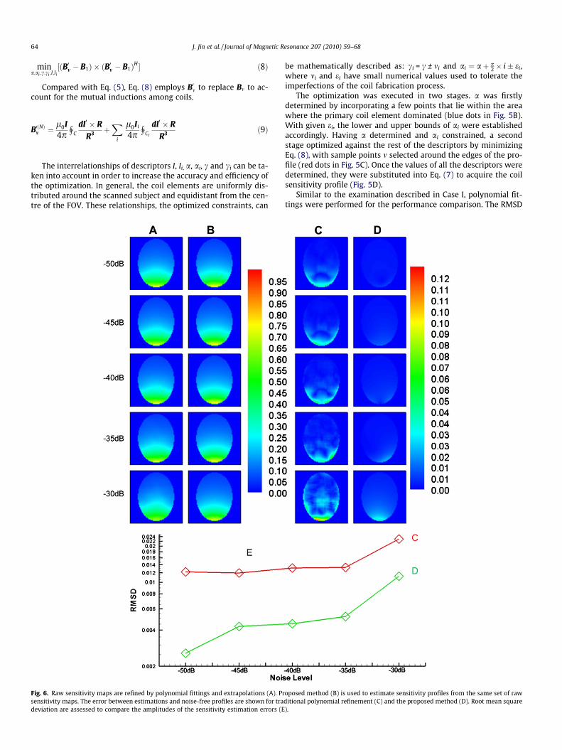
In Case II, the same set of analyses was used to simulate the sce-nario where a set of four coils acquired data simultaneously. Theresults, shown in Figs. 8 and 9, are similar to those in Case I, whichindicate that the optimization process, described by Eq. (7) andFig. 5, successfully constructed coil sensitivity profiles in the pres-ence of mutual coupling. In Fig. 9D we can see that the superior

Fig. 8. Raw sensitivity maps are refined by polynomial fittings and extrapolations (A) andshown for traditional polynomial refinement (C) and the proposed method (D). Rootestimation errors (E).

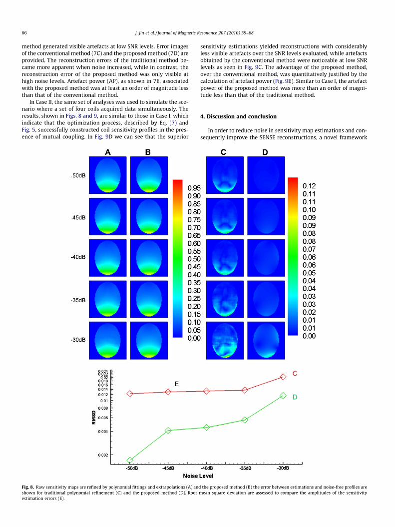
sensitivity estimations yielded reconstructions with considerablyless visible artefacts over the SNR levels evaluated, while artefactsobtained by the conventional method were noticeable at low SNRlevels as seen in Fig. 9C. The advantage of the proposed method,over the conventional method, was quantitatively justified by thecalculation of artefact power (Fig. 9E). Similar to Case I, the artefactpower of the proposed method was more than an order of magni-tude less than that of the traditional method.

4. Discussion and conclusion

In order to reduce noise in sensitivity map estimations and con-sequently improve the SENSE reconstructions, a novel framework

the proposed method (B) the error between estimations and noise-free profiles aremean square deviation are assessed to compare the amplitudes of the sensitivity

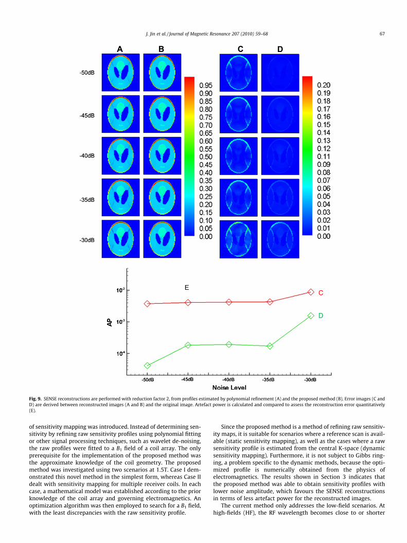
Fig. 9. SENSE reconstructions are performed with reduction factor 2, from profiles estimated by polynomial refinement (A) and the proposed method (B). Error images (C andD) are derived between reconstructed images (A and B) and the original image. Artefact power is calculated and compared to assess the reconstruction error quantitatively(E).

J. Jin et al. / Journal of Magnetic Resonance 207 (2010) 59–68 67

of sensitivity mapping was introduced. Instead of determining sen-sitivity by refining raw sensitivity profiles using polynomial fittingor other signal processing techniques, such as wavelet de-noising,the raw profiles were fitted to a B1 field of a coil array. The onlyprerequisite for the implementation of the proposed method wasthe approximate knowledge of the coil geometry. The proposedmethod was investigated using two scenarios at 1.5T. Case I dem-onstrated this novel method in the simplest form, whereas Case IIdealt with sensitivity mapping for multiple receiver coils. In eachcase, a mathematical model was established according to the priorknowledge of the coil array and governing electromagnetics. Anoptimization algorithm was then employed to search for a B1 field,with the least discrepancies with the raw sensitivity profile.

Since the proposed method is a method of refining raw sensitiv-ity maps, it is suitable for scenarios where a reference scan is avail-able (static sensitivity mapping), as well as the cases where a rawsensitivity profile is estimated from the central K-space (dynamicsensitivity mapping). Furthermore, it is not subject to Gibbs ring-ing, a problem specific to the dynamic methods, because the opti-mized profile is numerically obtained from the physics ofelectromagnetics. The results shown in Section 3 indicates thatthe proposed method was able to obtain sensitivity profiles withlower noise amplitude, which favours the SENSE reconstructionsin terms of less artefact power for the reconstructed images.

The current method only addresses the low-field scenarios. Athigh-fields (HF), the RF wavelength becomes close to or shorter

68 J. Jin et al. / Journal of Magnetic Resonance 207 (2010) 59–68

than the anatomy being scanned and the geometry of the RF coil.The loading effects and coil-tissue interactions lead to non-uniformdistributions of the RF current in the coil [25–28]. These effects areno longer negligible and invalidate the use of Biot–Savart Law forthe calculation of the B1 fields at HFs and it requires full-wave elec-tromagnetic solutions. In these cases, a detailed RF coil model hasto be developed to consider the variations of RF currents (includingamplitudes and phases) and array coupling; fortunately, hybridnumerical approaches [27,28] can be used to handle the involvedelectromagnetic problem. In addition, the HF Bþ1 and B�1 behave dif-ferently and therefore caution should be exercised when relatingthe reception sensitivity to the transmission sensitivity of the samecoil using the reciprocity theorem. Currently we are working onextending the proposed concept for HF applications including par-allel reconstruction and parallel transmission [29–32].

References

[1] F. Wiesinger, P.F. Van de Moortele, G. Adriany, N. De Zanche, K. Ugurbil, K.P.Pruessmann, Potential and feasibility of parallel MRI at high field, NMR inBiomedicine 19 (2006) 368–378.

[2] K.P. Pruessmann, M. Weiger, M.B. Scheidegger, P. Boesiger, SENSE: sensitivityencoding for fast MRI, Magnetic Resonance in Medicine 42 (1999) 952–962.

[3] K.P. Pruessmann, M. Weiger, P. Bornert, P. Boesiger, Advances in sensitivityencoding with arbitrary k-space trajectories, Magnetic Resonance in Medicine46 (2001) 638–651.

[4] M.A. Griswold, P.M. Jakob, R.M. Heidemann, M. Nittka, V. Jellus, J.M. Wang, B.Kiefer, A. Haase, Generalized autocalibrating partially parallel acquisitions(GRAPPA), Magnetic Resonance in Medicine 47 (2002) 1202–1210.

[5] M.A. Griswold, P.M. Jakob, M. Nittka, J.W. Goldfarb, A. Haase, Partially parallelimaging with localized sensitivities (PILS), Magnetic Resonance in Medicine 44(2000) 602–609.

[6] W.E. Kyriakos, L.P. Panych, D.F. Kacher, C.F. Westin, S.M. Bao, R.V. Mulkern, F.A.Jolesz, Sensitivity Profiles from an Array of Coils for Encoding andReconstruction in Parallel (SPACE RIP), John Wiley & Sons Inc., Denver,Colorado, 2000. pp. 301–308.

[7] P.M. Jakob, M.A. Grisowld, R.R. Edelman, D.K. Sodickson, AUTO-SMASH: a self-calibrating technique for SMASH imaging, Magnetic Resonance Materials inPhysics, Biology and Medicine 7 (1998) 42–54.

[8] M.A. Griswold, P.M. Jakob, Q. Chen, J.W. Goldfarb, W.J. Manning, R.R. Edelman,D.K. Sodickson, Resolution enhancement in single-shot imaging usingsimultaneous acquisition of spatial harmonics (SMASH), Magnetic Resonancein Medicine 41 (1999) 1236–1245.

[9] R.M. Heidemann, M.A. Griswold, A. Haase, P.M. Jakob, VD-AUTO-SMASHimaging, Magnetic Resonance in Medicine 45 (2001) 1066–1074.

[10] D.K. Sodickson, C.A. McKenzie, A generalized approach to parallel magneticresonance imaging, Medical Physics 28 (2001) 1629–1643.

[11] Z. Chen, J. Zhang, R. Yang, P. Kellman, L.A. Johnston, G.F. Egan, IIR GRAPPA forparallel MR image reconstruction, Magnetic Resonance in Medicine 63 (2009)502–509.

[12] W.S. Hoge, D.H. Brooks, Using GRAPPA to improve autocalibrated coilsensitivity estimation for the SENSE family of parallel imagingreconstruction algorithms, Magnetic Resonance in Medicine 60 (2008) 462–467.

[13] C.A. McKenzie, E.N. Yeh, M.A. Ohliger, M.D. Price, D.K. Sodickson, Self-calibrating parallel imaging with automatic coil sensitivity extraction,Magnetic Resonance in Medicine 47 (2002) 529–538.

[14] F.H. Lin, Y.J. Chen, J.W. Belliveau, L.L. Wald, A wavelet-based approximation ofsurface coil sensitivity profiles for correction of image intensityinhomogeneity and parallel imaging reconstruction, Human Brain Mapping19 (2003) 96–111.

[15] L. Ying, J. Sheng, Joint Image reconstruction and sensitivity estimation inSENSE (JSENSE), Magnetic Resonance in Medicine 57 (2007) 1196–1202.

[16] D.I. Hoult, The principle of reciprocity in signal strength calculations – amathematical guide, Concepts in Magnetic Resonance Part A 12 (2000) 173–187.

[17] T.S. Ibrahim, Analytical approach to the MR signal, Magnetic Resonance inMedicine 54 (2005) 677–682.

[18] P.B. Roemer, W.A. Edelstein, C.E. Hayes, S.P. Souza, O.M. Mueller, The NMRphased-array, Magnetic Resonance in Medicine 16 (1990) 192–225.

[19] J.M. Wang, A. Reykowski, J. Dickas, Calculation of the signal-to-noise ratio forsimple surface coils and arrays of coils, IEEE Transactions on BiomedicalEngineering 42 (1995) 908–917.

[20] F. Liu, A. Trakic, H.S. Lopez, Q. Wei, M. Fuentes, E. Weber, S. Crozier, Reverse-engineering of gradient coil designs based on experimentally measuredmagnetic fields and approximate knowledge of coil geometry-application inexposure evaluations, Concepts in Magnetic Resonance Part B: MagneticResonance Engineering 35B (2009) 32–43.

[21] M.A. Griswold, F. Breuer, M. Blaimer, S. Kannengiesser, R.M. Heidemann, M.Mueller, M. Nittka, V. Jellus, B. Kiefer, P.M. Jakob, Autocalibrated coil sensitivityestimation for parallel imaging, NMR in Biomedicine 19 (2006) 316–324.

[22] J.D. Jackson, Classical Electrodynamics, 3rd ed., Wiley, New York, 1925.[23] D.K. Cheng, Field and Wave Electromagnetics, second ed., Addison-Wesley,

Pub Co, Berlin, 1917.[24] T.F. Coleman, Y. Li, An interior trust region approach for nonlinear

minimization subject to bounds, SIAM Journal on Optimization 6 (1996)418–445.

[25] T.S. Ibrahim, R. Lee, B.A. Baertlein, Y. Yu, P.M.L. Robitaille, Computationalanalysis of the high pass birdcage resonator: finite difference time domainsimulations for high-field MRI, Magnetic Resonance Imaging 18 (2000) 835–843.

[26] T.S. Ibrahim, C. Mitchell, R. Abraham, P. Schmalbrock, In-depth study of theelectromagnetics of ultrahigh-field MRI, NMR in Biomedicine 20 (2007) 58–68.

[27] F. Liu, B.L. Beck, B. Xu, J.R. Fitzsimmons, S.J. Blackband, S. Crozier, Numericalmodeling of 11.1T MRI of a human head using a MoM/FDTD method, Conceptsin Magnetic Resonance Part B: Magnetic Resonance Engineering 24B (2005)28–38.

[28] F. Liu, S. Crozier, Electromagnetic fields inside a lossy. Multilayered sphericalhead phantom excited by MRI coils: models and methods, Physics in Medicineand Biology 49 (2004) 1835–1851.

[29] W.A. Grissom, C.Y. Yip, S.M. Wright, J.A. Fessler, D.C. Noll, Additive anglemethod for fast large-tip-angle RF pulse design in parallel excitation, MagneticResonance in Medicine 59 (2008) 779–787.

[30] D. Xu, K.F. King, Y.D. Zhu, G.C. McKinnon, Z.P. Liang, A noniterative method todesign large-tip-angle multidimensional spatially-selective radio frequencypulses for parallel transmission, Magnetic Resonance in Medicine 58 (2007)326–334.

[31] Y. Zhu, Parallel excitation with an array of transmit coils, Magnetic Resonancein Medicine 51 (2004) 775–784.

[32] U. Katscher, P. Bornert, C. Leussler, J.S. Van den Brink, Transmit SENSE,Magnetic Resonance in Medicine 49 (2003) 144–150.