Development of an Electromagnet Excited Mass–Pendulum SystemModeling and Control Laboratory Experiment — Theory And Test

Kelly R. Austin and John R. Wagner, Ph.D., P.E.

Abstract— An electromagnet excited mass–pendulum systemwith attached spring and damper elements is introduced as asenior and graduate level engineering laboratory experiment.This laboratory offers mechanical, electrical, and control engi-neering challenges to the students. The derivation of the coupledequations of motion is developed using both Newtonian andLagrangian approaches. The system is pendulum actuated by apowerful electromagnet for which the magnetic force is modeledby a magnetostatic forcing function. Representative numericaland experimental results are presented which validate themathematical model. Further, the bench top experiment offershands-on opportunities for the students. The numerical resultsagree within 2% to 20% of the experiments.

I. INTRODUCTIONThe mass–pendulum system with spring and damper el-

ements is a classical coupled dynamics problem that maybe posed to engineering students. The dynamics of themass-pendulum system, somewhat similar to the suspensionspring pendulum interfaces on tower clock mechanisms,offers the challenge of working with a coupled systemwhich is subjected to non-linear motion. The system sharessome similarities with the underactuated cart driven invertedpendulum and pendulum driven cart mechanical systems withrespective swing-up stabilizing and tracking problems [1][2].

Due to the inertial coupling of the masses, this two masssystem also offers an optimization problem in vibrationreduction. As a passive tuned mass damper, the pendulumwas found to be useful in reducing steady state and lowseismic motion [3]. The pendulum has also been researchedas an active mass damper against wind and low seismicmotion [4]. Both of these have the challenge of workingwith a system that is subject to non-linear and chaotic motiondepending on system damping and forcing frequency [5].

This laboratory experiment incorporates fundamental en-gineering concepts while working with a nonlinear physicalsystem. Students mathematically model the system by eithera direct application of Newton’s second law or by use ofLagrange’s equations for education purposes. The model isthen verified by numerical simulation of the free response ofthe coupled system which requires analyzing the uncoupledand coupled motion of the masses to determine the systemparameter values. Calculating the system parameters from thephysical system incorporates sensor integration and calibra-tion, data acquisition, signal processing, and data analysis.

The actuator used is a powerful electromagnet whichmust be incorporated into the physical system to drive the

K. Austin is with Eaton Aerospace Group, Jackson, MS 39206, USAProfessor Wagner is with Clemson University, Clemson, SC 29634, USA

pendulum based on the real time motion of the coupledsystem. By mathematically modeling the magnitude of theelectromagnet’s magnetic force, the forced response of themass-pendulum mathematical model can be simulated andcompared to the forced response of the physical system. Withthe physical system and validated model, the linear and non-linear motion of the coupled system can be experimentallyand analytically evaluated to control the system response.

II. MATHEMATICAL MODELS

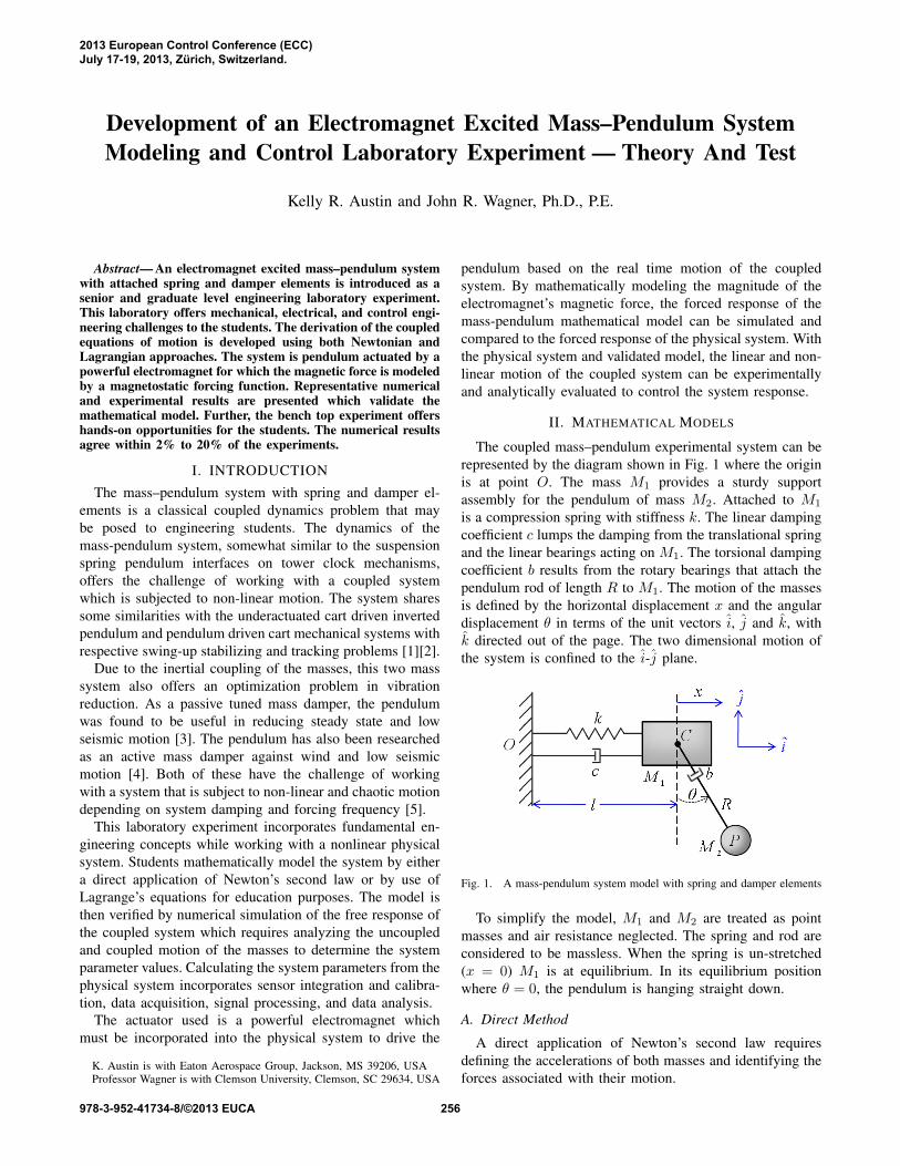
The coupled mass–pendulum experimental system can berepresented by the diagram shown in Fig. 1 where the originis at point O. The mass M1 provides a sturdy supportassembly for the pendulum of mass M2. Attached to M1

is a compression spring with stiffness k. The linear dampingcoefficient c lumps the damping from the translational springand the linear bearings acting on M1. The torsional dampingcoefficient b results from the rotary bearings that attach thependulum rod of length R to M1. The motion of the massesis defined by the horizontal displacement x and the angulardisplacement θ in terms of the unit vectors i, j and k, withk directed out of the page. The two dimensional motion ofthe system is confined to the i-j plane.

Fig. 1. A mass-pendulum system model with spring and damper elements

To simplify the model, M1 and M2 are treated as pointmasses and air resistance neglected. The spring and rod areconsidered to be massless. When the spring is un-stretched(x = 0) M1 is at equilibrium. In its equilibrium positionwhere θ = 0, the pendulum is hanging straight down.

A. Direct Method

A direct application of Newton’s second law requiresdefining the accelerations of both masses and identifying theforces associated with their motion.

2013 European Control Conference (ECC)July 17-19, 2013, Zürich, Switzerland.

978-3-952-41734-8/©2013 EUCA 256

1) Kinematics of Masses M1 and M2: The kinematicequations of M1 are

~rc = xi (1)

~vc = ~rc = xi (2)

~ac = ~vc = ~rc = xi (3)

where position ~rc, velocity ~vc, and acceleration ~ac describethe motion of the mass which is constrained to move hor-izontally. The distance l from O to C at x = 0 has beenneglected since it does not appear in the derivatives.

The kinematic equations of M2, which has combinedrotational and translational motion, are

~rp = xi+R sin θi−R cos θj (4)

~vp = ~rp = xi+Rθ cos θi+Rθ sin θj (5)

~ap = ~vp = ~rp = xi+R(θ cos θ − θ2 sin θ

)i+

R(θ sin θ + θ2 cos θ

)j.

(6)

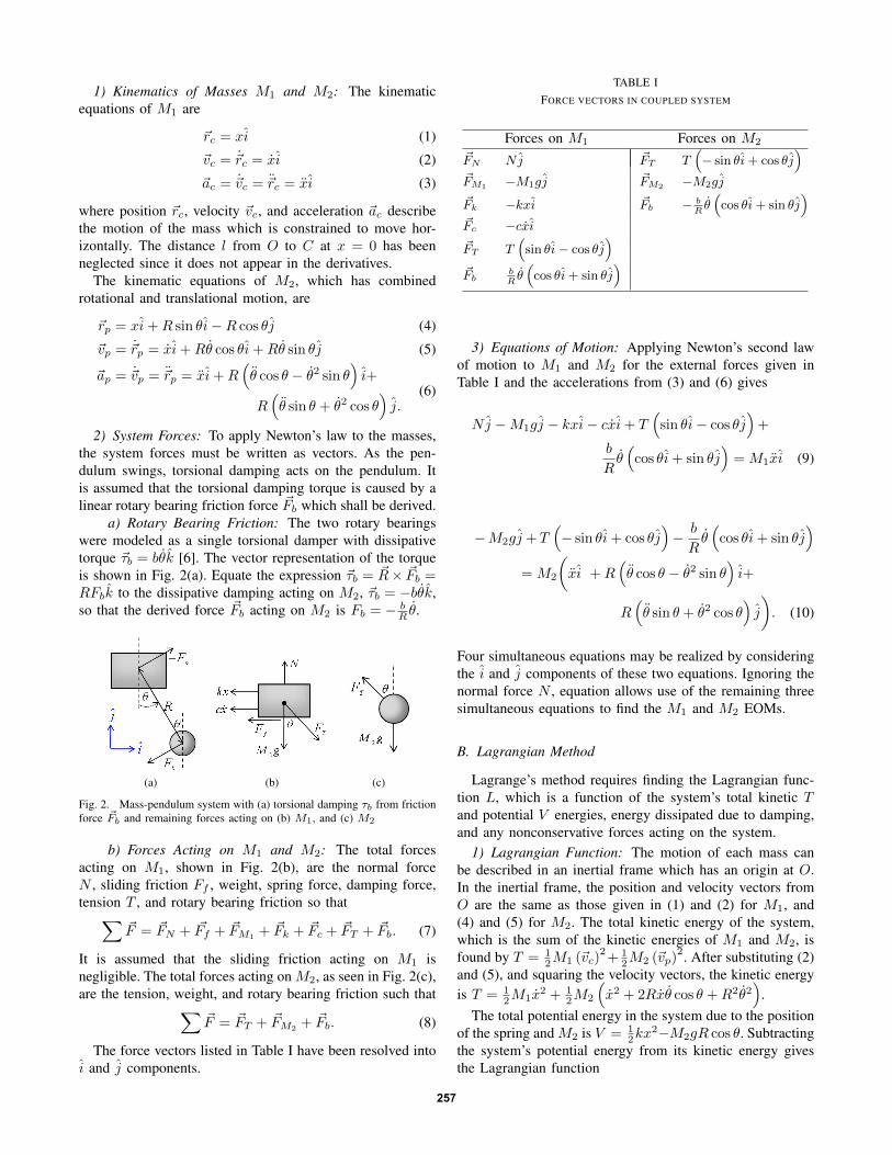
2) System Forces: To apply Newton’s law to the masses,the system forces must be written as vectors. As the pen-dulum swings, torsional damping acts on the pendulum. Itis assumed that the torsional damping torque is caused by alinear rotary bearing friction force ~Fb which shall be derived.

a) Rotary Bearing Friction: The two rotary bearingswere modeled as a single torsional damper with dissipativetorque ~τb = bθk [6]. The vector representation of the torqueis shown in Fig. 2(a). Equate the expression ~τb = ~R× ~Fb =RFbk to the dissipative damping acting on M2, ~τb = −bθk,so that the derived force ~Fb acting on M2 is Fb = − b

R θ.

(a) (b) (c)

Fig. 2. Mass-pendulum system with (a) torsional damping τb from frictionforce ~Fb and remaining forces acting on (b) M1, and (c) M2

b) Forces Acting on M1 and M2: The total forcesacting on M1, shown in Fig. 2(b), are the normal forceN , sliding friction Ff , weight, spring force, damping force,tension T , and rotary bearing friction so that∑

~F = ~FN + ~Ff + ~FM1 +~Fk + ~Fc + ~FT + ~Fb. (7)

It is assumed that the sliding friction acting on M1 isnegligible. The total forces acting on M2, as seen in Fig. 2(c),are the tension, weight, and rotary bearing friction such that∑

~F = ~FT + ~FM2+ ~Fb. (8)

The force vectors listed in Table I have been resolved intoi and j components.

TABLE IFORCE VECTORS IN COUPLED SYSTEM

Forces on M1 Forces on M2

~FN Nj ~FT T(− sin θi+ cos θj

)~FM1 −M1gj ~FM2 −M2gj

~Fk −kxi ~Fb − bRθ(cos θi+ sin θj

)~Fc −cxi~FT T

(sin θi− cos θj

)~Fb

bRθ(cos θi+ sin θj

)

3) Equations of Motion: Applying Newton’s second lawof motion to M1 and M2 for the external forces given inTable I and the accelerations from (3) and (6) gives

Nj −M1gj − kxi− cxi+ T(sin θi− cos θj

)+

b

Rθ(cos θi+ sin θj

)=M1xi (9)

−M2gj + T(− sin θi+ cos θj

)− b

Rθ(cos θi+ sin θj

)=M2

(xi +R

(θ cos θ − θ2 sin θ

)i+

R(θ sin θ + θ2 cos θ

)j

). (10)

Four simultaneous equations may be realized by consideringthe i and j components of these two equations. Ignoring thenormal force N , equation allows use of the remaining threesimultaneous equations to find the M1 and M2 EOMs.

B. Lagrangian Method

Lagrange’s method requires finding the Lagrangian func-tion L, which is a function of the system’s total kinetic Tand potential V energies, energy dissipated due to damping,and any nonconservative forces acting on the system.

1) Lagrangian Function: The motion of each mass canbe described in an inertial frame which has an origin at O.In the inertial frame, the position and velocity vectors fromO are the same as those given in (1) and (2) for M1, and(4) and (5) for M2. The total kinetic energy of the system,which is the sum of the kinetic energies of M1 and M2, isfound by T = 1

2M1 (~vc)2+ 1

2M2 (~vp)2. After substituting (2)

and (5), and squaring the velocity vectors, the kinetic energyis T = 1

2M1x2 + 1

2M2

(x2 + 2Rxθ cos θ +R2θ2

).

The total potential energy in the system due to the positionof the spring and M2 is V = 1

2kx2−M2gR cos θ. Subtracting

the system’s potential energy from its kinetic energy givesthe Lagrangian function

257

L = T − V =1

2M1x

2 +1

2M2x

2 +M2Rxθ cos θ+

1

2M2R

2θ2 − 1

2kx2 +M2Rg cos θ. (11)

2) Lagrange’s Equations: The equation describing themotion of a generalized coordinate qi is determined by

d

dt

(∂L

∂qi

)− ∂L

∂qi+∂D

∂qi= Qi (i = 1, 2, · · · ) (12)

where the Lagrangian L is given in (11), the energy dissi-pated due to damping is given for the damping coefficient ciat velocity qi by Rayleigh’s dissipation function D = 1

2ciq2i ,

and the generalized force Qi encompasses the applied forceand any non conservative force such as sliding friction [7].

The EOM for M1 is found by evaluating (12) for thecoordinate q1 = x, where the partial derivatives of (11) aretaken with respect to x and x, and Rayleigh’s dissipationfunction for the damping of x is D = 1

2cx2. Evaluating (12)

for q2 = θ gives the dynamics for M2. The partial derivativesin (11) are taken with respect to θ and θ, and D = 1

2bθ2 is

Rayleigh’s dissipation function for the damping in θ.The EOM for M1 and M2 found from Lagrange’s method

are the same as those found by the direct method, which canbe solved for x and θ respectively to give the EOM for themass-pendulum system [3][8]

x =1

M1 +M2

(M2Rθ

2 sin θ −M2Rθ cos θ − cx− kx)

(13)

θ =1

M2R

(−M2x cos θ −M2g sin θ −

b

Rθ

). (14)

C. Model of Magnetic Force

The magnetic effect of the electromagnet is characterizedin terms of magnetic flux density ~B. The magnetic flux φ isfound by integrating the flux density over the surface areathat the flux lines pass through. The electromagnet vectorfield properties can be treated as scalars by viewing theelectromagnet and the attracted load, M2, as a “magneticcircuit” analogous to a resistive electric circuit [9].

It is assumed that the electromagnet is in an electrostaticstate powered by the direct current i, and the N coil turnson the tightly wound electromagnet core are linked by thegenerated magnetic field lines so the magnetomotive force(mmf) becomes F = Ni. The magnetic flux φ producedby the mmf follows a mean closed path of length l througheach material comprising the magnetic circuit and must beentirely confined in the circuit.

The reluctance R is a material property defined as lthrough the material divided by the product of the material’spermeability µ and cross sectional area, R = l/(µA). The µof the material can be factored into the permeability of freespace µ0 and the material’s dimensionless relative permeabil-ity µr. For a magnetostatic measurement, µ is also referred toas the absolute permeability. While µ0 is a magnetic constant,

the relative permeability of a ferromagnetic material dependson the absolute permeability, which depends on the degreeto which the material is magnetized [10]. Using an analogybetween voltage and magnetomotive force and the definitionof R, the mmf becomes

F = Ni = φR = φl

µA= φ

l

µ0µrA.(15)

For this approximation of the magnetic force, the magneticcircuit includes a solid core electromagnet and movable loadM2 separated on both sides by equal sized air gaps. The fluxmean path is considered to be through the core, a length oflC , across the air gap, a length of xg , through the load, alength of lL, and back across the air gap to the core. Thetotal reluctance is a function of xg , stated as

R(xg) =lC

µ0µrCAC+ 2

xgµ0µrgAg

+lL

µ0µrLAL. (16)

where µrC , µrg , and µrL are the relative permeabilities ofthe core, air gap, and load, and AC , Ag , and AL are thecross sectional areas of the core, air gap, and load.

The magnetic force f acting on M2 can be approximatedby considering the work done by the current in the coiland the work required to move M2 from a position xgmeters away. The derived forcing function is |f(xg)| =

− 12φ

2 dR(xg)dxg

[9]. The derivative of the reluctance in (16)

with respect to xg is dR(xg)dxg

= 2µ0µrgAg

, and the flux from

(15) is φ = NiR(xg)

. The magnetic force, in Newtons, iscalculated from the function

|f(xg)| = −(Ni)2

R2(xg)µ0µrgAg(17)

where R(xg) is calculated from (16) for xg in meters. Thisforcing function assumes that no fringing of the magneticflux lines occurs in the air gap, in which the flux lines leavingthe core bow out and then come back into the load. Theair gap cross sectional area considering fringing AgF wasassumed to be a function of xg , where AgF (xg) = (

√Ag +

xg)2 and Ag is the air gap cross sectional area neglecting

fringing. Considering this term in (16) and the derivative ofthis expression with respect to xg , gives a magnetic forcefunction |fF (xg)|, which approximates for the fringing ofthe magnetic flux lines in the air gap, as

|fF (xg)| =−(Ni)2

(xg −A

12g

)(xg +A

12g

)−3 2xg√

µ0(xg+A

12g

)2 +lCµrLAL+lLµrCAC√

µ0µrCACAL

2 . (18)

The displacement xg of M2 from the electromagnet andthe approximated magnetic force f(xg) is illustrated inFig. 3, where the equilibrium position of the system is atthe x, y axes, and the electromagnet is positioned ±xm withrespect to the y -axis. The positive or negative horizontal

258

Fig. 3. The magnetic force f(xg) of the electromagnet, positioned ±xmfrom the equilibrium, acts at angle ψ on the pendulum mass located at ahorizontal distance D over the air gap displacement xg

distance D of M2 from the electromagnet is found byD = x + R sin θ − xm, where the sign of D indicates towhich side of the electromagnet M2 is. From Fig. 3, themagnitude of the displacement xg is calculated by

|xg| =√(x+R sin θ − xm)2 + (R−R cos θ)2. (19)

The magnetic force produces a torque on the pendulum.This torque is represented as a generalized force in (12) forthe coordinate θ as Qθ = ~Fθ · ∂~rθ∂θ , where ~rθ is given in (4).The magnetic force vector applied to M2 at an angle ψ fromthe vertical is ~Fθ = −f(xg) sinψi − f(xg) cosψj. Findingψ = tan−1

(D

R−R cos θ

), the dot product of the force vector

and the partial derivative of (4) with respect to θ gives thegeneralized force acting on M2 as

Qθ = −f(xg)R sin(θ + ψ). (20)

III. ANALYSIS OF SYSTEM PARAMETERS

By decoupling the motions of M1 and M2, the systemconstants can be analytically and experimentally estimated.The log decrement method was used to estimate the dampingratios of M1 and M2, which are assumed to be underdamped.

The general solution of M1 motion is

x(t) = Ae−ζωnt sin(ωn√1− ζ2 t+ β

), (21)

with damping ratio ζ = c/(2√M1k

), undamped natural

frequency ωn =√

kM1

, and damped natural frequency ωd =

ωn√1− ζ2 [11].

Assuming small angle motion,the general solution of theM2 motion is defined by [11]

θ(t) = Beζpωnp t sin(ωnp

√1− ζ2p t+ βp

)(22)

with undamped natural frequency ωnp =√

gR and damping

ratio ζp = b/(2M2R2)√

g/R[11]. The torsional damping in the

pivot point at C causes M2 to oscillate at a damped naturalfrequency ωdp = ωnp

√1− ζ2p .

For the uncoupled free response of M1, the logarithmicdecrement δ uses the natural logarithm of successive ampli-tude ratios separated by n periods of length P , [6]

δ =1

nln

x(t)

x(t+ nP ). (23)

Using (21) and the definition P = 2πωd

in this equation, M1

damping ratio is found as ζ = δ√4π2+δ2

. Using the sameprocedure, (22) can determine ζp for the motion of M2.

IV. EXPERIMENTAL SYSTEM

The bench top laboratory experiment shown in Fig. 4 wasdesigned to encourage student interactions with the system.The sensors include a full bridge beam load cell (Omega, partnumber LCL-010) and a quadrature optical encoder kit (USDigital, part number E2-1024-N-DD-B). The output signalof the load cell is amplified by a strain gauge amplifier(Omega, part number DRC-4710) which also supplies the (5-12)VDC bridge supply to the load cell. The optical encoderkit consists of a 1-inch rotary code wheel with 1024 countsper revolution per channel, read by a HEDS-9100 opticalencoder module. The electromagnet, made of 1018 lowcarbon steel, is wound with 22-AWG magnet wire. Thecurrent i is supplied by an external 15VDC power supplycontrolled by a MOSFET switch using a dSpace controllerboard DS1103 and a CLP1103 connector panel.

Fig. 4. Mass-pendulum system with integrated sensors and electromagnet

V. ELECTROMAGNET CONTROL

The controller should initiate and maintain pendulummotion for general purpose vibration studies. Using the elec-tromagnet to activate the motion of M2 requires identifyingthe mass’s direction of motion and position with respect tothe fixed position of the electromagnet. The electromagnetdisplacement from the equilibrium position, xm, can have amaximum value of 11.4cm measured from the electromagnetcenter. To activate motion, the electromagnet should turn on

259

when M2 is swinging toward it, and turn off the moment thependulum swings past it so that the magnetic field does notslow the motion.

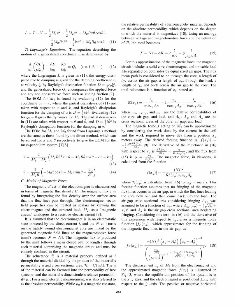
In the physical system, the control logic is incorporatedin the Simulink model with dSpace and Control Desk. Thecontrol logic is listed in Table II. The logic inputs of theexperimental system identify the sets of conditions that mustbe true for the electromagnet to be activated. The logic inputsof the simulated system identify the conditions that must betrue for the positive or negative torque to be calculated forthe value of xg and applied to the system. If the first setof conditions listed for both the experimental and simulatedsystems is true, the pendulum is approaching the right sideof the electromagnet, as shown in Fig. 3. The second setof conditions listed for both system then signals that thependulum is approaching the left side of the electromagnet.

TABLE IISYSTEM LOGIC CONDITIONS FOR OUTPUT SIGNAL ACTIVATION

Definition of Logic Input Conditions: u1 to u5u1 term sgn

(d|xg|dt

)u2 term sgn(D)

u3 term sgn(θ)u4 term Interval Test, xg > |0.01m|u5 term Interval Test, 0.01m < xg < 0.10m

Logic Inputs Experimental System Outputu1 < 0, u2 > 0, u3 < 0, and u4=1 Onu1 < 0, u2 < 0, u3 > 0, and u4=1 OnLogic Inputs Simulated System Outputu1 < 0, u2 > 0, u3 < 0, and u5=1 −Qθu1 < 0, u2 < 0, u3 > 0, and u5=1 +Qθ

VI. NUMERICAL AND EXPERIMENTAL RESULTS

The free and forced responses of the experimental andsimulated systems were compared by first determining theexperimental system parameters for the simulation. This alsorequired estimating the uncertain electromagnet parametersto derive the magnetic forcing function. All system parame-ters are listed in Table III.

A. Free Response

The free response of the mass-pendulum system wasanalyzed for various combinations of initial conditions (ICs)and compared to the free response of (13) and (14) in Matlabfor the same ICs. The system free response for which theinitial positions of M1 and M2 are opposed to each otheris shown in Fig. 5(a)–(d). Due to friction, the oscillationsin the physical system quickly decrease with all perceptiblemotion in M1 ceasing approximately 15sec before M2 stopsoscillating. As can be seen from the plots, by accountingfor the friction force (Ff = µkW sgn(x) from the linearbearings in M1, where µk is the kinetic friction coefficientand W is the weight) the simulated response gives a goodrepresentation of the system motion.

TABLE IIISYSTEM PARAMETERS

Parameter,Variable ValueElectromagnet Parameters

Permeability of free space, µ0 4π × 10−7 H/mPermeability of steel, µr 70±10Permeability of air, µrg 1Mean flux path through core, lC 0.203mMean flux path through load, lL 5.71×10−2mCore cross sectional area, AC 5.07×10−4m2

Load cross sectional area, AL 2.74×10−3m2

Air gap cross sectional area, Ag 1.27×10−3m2

Turns on electromagnet, N 864turnsCurrent, i 2.67A

M1 ParametersMass (including encoder) 0.950kgDamping ratio, ζ 0.0904± 0.0363Damping coefficient, c (1.67± 0.71)N·s/mSpring constant, k (90.1± 13.4)N/mNatural frequency, ωn (9.74± 0.35)rad/sFriction coefficient, µk 0.015± 0.004

M2 ParametersMass (includes rod mass) 1.363 kgRod length, R 0.341 mDamping ratio, ζp (1.89±0.89)·10−4

Damping coefficient, b (3.18±1.54)·10−4N·m·sNatural frequency, ωnp (5.32± 0.01)rad/s

Fig. 5. Comparison of the physical (—) and simulated (- - -) systemresponses due to initial conditions θ0 = −π/6rad and x0 = 0.05m for (a)M1, (b) M2, and (c and d) motion of M2 with respect to M1

260

B. Forced Response

In the experimental system, the forced response wasinvestigated for three positions of the electromagnet, xm =(1) − 4cm, (2) −7.5cm, and (3) −11.4cm (the response ofthe system for positive values of xm placements was found tobe similar). To compare the interaction between the massesand the application of the magnetic force, the electromagnetinduced motion of M2 was found, keeping M1 fixed, andthe system’s coupled response was found in which M1 wasunconstrained. A summary of the forced system response forthe experimental and simulated systems is shown in TablesIV and V. For the case in which M1 was held stationary, theRMS amplitude and minimum and maximum amplitudes ofM2 are given with its oscillating frequency.

When M1 is not constrained, the RMS amplitude and theminimum and maximum amplitudes of both M1 and M2

were determined for a 10sec sample time after the initialtransients died out. Only the oscillating frequency of M2 islisted since the masses oscillate at the same frequency. Forthe electromagnet positioned furthest away, the oscillatingfrequency of M1 could not be determined.

TABLE IVEXPERIMENTAL SYSTEM FORCED RESPONSE

M1 Held Stationary [0–100]secxm θrms θmin θmax ωM2

(rad) (rad) (rad) (rad/s)1 0.407 −0.825 0.822 5.27

2 0.383 −0.755 0.755 5.27

3 0.237 −0.542 0.542 5.32M1 Free to Move [90–100]sec

xm xrms xmin xmax θrms θmin θmax ωM2

(cm) (cm) (cm) (rad) (rad) (rad) (rad/s)1 1.62 −2.94 1.90 0.113 −0.158 0.164 4.50

2 1.22 −1.99 1.32 0.086 −0.144 0.123 4.16

3 0.267 −0.497 −0.155 0.009 −0.017 0.015 5.26

The simulated system response is representative of theresponse of the physical system up to approximately θ =π4 rad for all tests. For Test 1, in which the electromagnet ispositioned at −4cm, the physical and the simulated systemreach a maximum amplitude of π

4 in approximately 90sec.The average percent difference between the amplitudes of thetwo plots for [0 − 90]sec is 3.1%. For Test 2, the physicaland simulated system reach π

4 in approximately 100sec, withan average percent difference in their amplitudes of 11.0%.For the electromagnet positioned furthest away, Test 3, M2

reaches π4 in 215sec in the physical response, and 230sec in

the simulated. The percent difference between the plots forthe first 100sec of motion is 7.7%.

When M1 is not fixed, per Tables IV and V, the motionof M1 greatly reduces the amplitude of the pendulum’soscillations for the same force. Starting with a small initialcondition, each mass reaches steady state oscillation within

TABLE VSIMULATED SYSTEM FORCED RESPONSE

M1 Held Stationary [0–100]secxm θrms θmin θmax ωM2

(rad) (rad) (rad) (rad/s)1 0.400 −0.809 0.806 5.23

2 0.369 −0.766 0.768 5.27

3 0.244 −0.528 0.525 5.32M1 Free to Move [90–100]sec

xm xrms xmin xmax θrms θmin θmax ωM2

(cm) (cm) (cm) (rad) (rad) (rad) (rad/s)1 1.88 −3.05 1.99 0.0883 −0.139 0.132 4.22

2 1.42 −2.20 2.13 0.0943 −0.179 0.105 3.84

3 0.0228 −0.0195 0.0312 0.0202 −0.0293 0.0278 5.37

five seconds. Compared to the pendulum motion when M1 isheld stationary, when the pivot point of an oscillating masshas allowable motion, the influence of the driving force onthe mass is damped. The motion of M1, which is constrainedby the attached spring, effectively limits the motion of M2.Thus a much larger force would be required to increase theoscillating amplitudes of the masses.

VII. CONCLUSION

This mass–pendulum laboratory experiment provides en-gineering students an opportunity to model and investigatea coupled dynamics problem. In using a physical system tovalidate a mathematical model, students gain experience insimulating a non-linear model, determining physical param-eter values, and acquiring and analyzing data.

REFERENCES

[1] K. Sakurama, S. Hara, and K. Nakano, “Swing-up Stabilization Con-trol of a Cart–Pendulum System via Energy Control and ControlledLagrangian Methods”, in Electrical Engineering in Japan, vol. 160,No. 4, 2007, pp. 617-623.

[2] H. Yu, Y. Liu, and T. Yang, “Closed-Loop Tracking Control of APendulum–Driven Cart–Pole Underactuated System”, Proc. IMechE,vol. 222 Part I, 2008, pp. 109-125.

[3] E. Matta and A. De Stefano, “Seismic Performance of Pendulum andTranslational Roof-garden TMDs”, in Mechanical Systems and SignalProcessing, vol. 23, No. 3, 2009, pp. 908-921.

[4] N. Abe, “Passive and Active Switching Vibration Control with Pen-dulum Type Damper”, in Proceedings of 2004 IEEE Conference onControl Applications Taipei, Taiwan, 2004, pp. 1034-1042.

[5] Y. Song, H. Sato, Y. Iwata, and T. Komatsuzaki, “The Response of ADynamic Vibration Absorber System with A Parametrically ExcitedPendulum”, Journal of Sound and Vibration, 2003, pp. 747-759.

[6] W. J. Palm III, System Dynamics, McGraw-Hill, New York, NY; 2005.[7] D. T. Greenwood, Principles of Dynamics, Prentice Hall, Englewood

Cliffs, NJ; 1988.[8] J. H. Williams, Jr., Fundamentals of Applied Dynamics, John Wiley

and Sons, Inc., New York, NY; 1996.[9] G. Rizzoni, Principles and Applications of Electrical Engineering, 5th

Ed., McGraw-Hill, New York, NY; 2007.[10] D. G. Fink and H. W. Beaty, Standard Handbook for Electrical

Engineers, 13th Ed., McGraw-Hill, New York, NY; 1993.[11] D. G. Zill and M. R. Cullen, Advanced Engineering Mathematics, 2nd

Ed., Jones and Bartlett Publishers, Inc., Boston, MA; 2000.

261