Embed Size (px)
Citation preview

An Efficient Forecasting Procedure for Kuhn-Tucker Consumer Demand Model Systems
Abdul Rawoof Pinjari (Corresponding Author) Department of Civil & Environmental Engineering
University of South Florida 4202 E. Fowler Ave., Tampa, FL 33620 Tel: 813-974- 9671, Fax: 813-974-2957
E-mail: [email protected]
and
Chandra Bhat The University of Texas at Austin
Dept of Civil, Architectural & Environmental Engineering 1 University Station C1761, Austin, TX 78712-0278
Tel: 512-471-4535, Fax: 512-475-8744 E-mail: [email protected]
July 2009
An Efficient Forecasting Procedure for Kuhn-Tucker Consumer Demand Model Systems
ABSTRACT
This paper proposes an efficient and accurate forecasting algorithm for the MDCEV model. The
algorithm builds on simple, yet insightful, analytical explorations with the Kuhn-Tucker
conditions of optimality that shed new light on the properties of the MDCEV model. For
specific, but reasonably general, functional forms of the consumption utility specification, the
algorithm circumvents the need to carry out any iterative constrained optimization procedures
that have hitherto been used for forecasting with Kuhn-Tucker (KT) demand model systems. The
non-iterative nature of the algorithm contributes significantly to its efficiency and accuracy.
Further, although developed in the context of the MDCEV model, the proposed algorithm can be
easily modified to be used in the context of other utility maximization-based Kuhn-Tucker (KT)
consumer demand model systems in the literature.
Simulation experiments highlight the efficiency of the algorithm compared to a
traditional iterative forecasting procedure. For example, to forecast the expenditures of 4000
households in 7 expenditure alternatives, for 500 sets of error term draws for each household, the
proposed algorithm takes less than 2 minutes. On the other hand, the iterative forecasting routine
would take around 2 days to do so.

1
1. INTRODUCTION
In several consumer demand situations, consumer behavior may be associated with the choice of
multiple alternatives simultaneously, along with a continuous choice component of “how much
to consume” for the chosen alternatives. Such multiple discrete-continuous choice situations are
being increasingly recognized and modeled in the recent literature in transportation, marketing,
and economics.
A variety of modeling frameworks have been used to analyze multiple discrete-
continuous choice situations. These can be broadly classified into: (1) statistically stitched
multivariate single discrete-continuous models (see, for example, Srinivasan and Bhat, 2006),
and (2) utility maximization-based Kuhn-Tucker (KT) demand systems (Hanemann, 1978;
Wales and Woodland, 1983; Kim et al., 2002; von Haefen and Phaneuf, 2005; Bhat, 2005 and
2008). Between the two approaches, the KT demand systems are more theoretically grounded in
that they employ a unified utility maximization framework for simultaneously analyzing the
multiple discrete and continuous choices. Further, these model systems accommodate
fundamental features of consumer behavior such as satiation effects through diminishing
marginal utility with increasing consumption.
The KT demand systems have been known for quite some time, dating back at least to the
research works of Hanemann (1978) and Wales and Woodland (1983). However, it is only in the
past decade that practical formulations of the KT demand system have appeared in the literature.
Recent applications include, but are not limited to, individual activity participation and time-use
studies (Bhat, 2005; Habib and Miller, 2009; Pinjari et al., 2008), household travel expenditure
analyses (Rajagopalan and Srinivasan, 2008; Ferdous et al., 2009), household vehicle ownership
and usage forecasting (Ahn et al., 2007; Fang, 2008; and Bhat et al., 2008), outdoor recreational
demand studies (von Haefen et al., 2004; and von Haefen and Phaneuf, 2005), and grocery
purchase analyses (Kim et al., 2002). As indicated by Vasqez-Lavín and Hanemann (2009), this
surge in interest may be attributed to the strong theoretical basis combined with the recent
developments in simulation techniques and econometric specifications that obviate the need for
simulation-based estimation.
Within the KT demand systems, the recently formulated multiple discrete-continuous
extreme value (MDCEV) model structure by Bhat (2005, 2008) is particularly attractive due to:

2
(1) its elegant closed-form probability expressions that simplify to the well-known multinomial
logit probabilities when each decision-maker chooses only one alternative (Bhat, 2005), and
(2) its functional form of utility specification that enables a clear interpretation of the utility
parameters and a convenient specification of the alternative attributes while maintaining the
property of weak complimentarity (Bhat, 2008). The MDCEV model has been applied to analyze
several of the choice situations identified earlier. Further, in recent papers, the basic MDCEV
framework has been expanded in several directions, including the incorporation of more general
error structures to allow flexible inter-alternative substitution patterns (Pinjari and Bhat, 2009;
Pinjari, 2009).
Despite the many developments and applications, a simple and practically feasible
forecasting procedure has not yet been developed for the MDCEV and other KT demand model
systems. This has severely limited the applicability of these models for practical forecasting and
other policy analysis purposes. Since the end-goal of model development and estimation is
generally forecasting and policy evaluation, development of a simple and easily applicable
forecasting procedure is a critical need in the area of KT demand model systems. This is not to
say that no forecasting procedures exist in the literature (see Section 2). However, the currently
available methods are either enumerative or iterative in nature, are not very accurate, and require
large computation times.
In the context of the above discussion, this paper develops an efficient, non-iterative
forecasting algorithm for the MDCEV model, which can also be applied for other KT demand
model systems in the literature. The algorithm builds on simple, yet insightful, analytical
explorations with the KT conditions that shed new light on the properties of the MDCEV model.
For specific (but reasonably general) forms of utility functions, the algorithm results in
analytically expressible consumptions obviating the need for approximation and minimizing the
room for inaccuracy. Even with more general utility functions, the properties of the MDCEV
model discovered in this paper can be used in designing efficient (albeit iterative) forecasting
algorithms.
The remainder of the paper is organized as follows. The next section highlights the nature
of the MDCEV forecasting problem and describes the currently used forecasting procedures in
the literature. Section 3 discusses some new properties of the MDCEV model. Building on these
properties, Section 4 presents the forecasting algorithm and some application results, along with

3
a discussion on how similar forecasting algorithms can be developed for other KT demand
system models. Section 5 concludes the paper.
2 FORECASTING WITH KT DEMAND MODEL SYSTEMS
The MDCEV and other KT demand modeling systems are based on a resource allocation
formulation. Specifically, it is assumed that the decision makers operate with a finite amount of
available resources (i.e., a budget), such as time or money. The decision-making mechanism is
assumed to be driven by an allocation of the limited amount of resources to consume various
goods/alternatives in such a way as to maximize the utility derived out of consumption. Further,
a stochastic utility framework is used to recognize the analyst’s lack of awareness of all factors
affecting consumer decisions. In addition, a non-linear utility function is employed to incorporate
important features of consumer choice making, including: (1) the diminishing nature of marginal
utility with increasing consumption, and (2) the possibility of consuming multiple
goods/alternatives as opposed to a single good/alternative. To summarize, the KT demand
modeling frameworks are based on a stochastic (due to stochastic utility framework), constrained
(due to the budget constraint), non-linear utility optimization formulation.
In most KT demand system models, the stochastic KT first order conditions of optimality
form the basis for model estimation. Specifically, an assumption that stochasticity (or
unobserved heterogeneity) is generalized extreme value (GEV) distributed leads to closed form
consumption probability expressions (Bhat 2005 and 2008; Pinjari 2009; von Haefen et al.,
2004) facilitating a straightforward maximum likelihood estimation of the model parameters.
Once the model parameters are estimated and given a budget amount for each decision-
maker, any forecasting or policy analysis exercise involves solving the stochastic, constrained,
non-linear utility maximization problem for optimal consumption quantities of the decision-
makers. Unfortunately, there is no straight-forward analytical solution to this problem; a
combination of simulation (to mimic the unobserved heterogeneity) and optimization (to solve
the constrained non-linear optimization problem) methods needs to be employed. That is, the
analyst must carry out constrained non-linear optimization to obtain the consumption forecasts at
each simulated value of unobserved heterogeneity (or stochasticity). Such conditional (on
unobserved heterogeneity) consumption forecasts evaluated over the entire simulated distribution

4
of unobserved heterogeneity are used to derive the distributions of unconditional consumption
forecasts.
To solve the conditional (on unobserved heterogeneity) constrained non-linear
optimization problem, the forecasting procedures used in the literature so far use either
enumerative or iterative optimization methods. The enumerative approach (used by Phaneuf et
al., 2000) involves enumeration of all possible sets of alternatives that the decision-maker can
potentially choose from the available set of alternatives. Specifically, if there are K available
choice alternatives, assuming not more than one essential Hicksian composite good (or outside
good)1, one can enumerate 2K-1 possible choice set solutions to the consumer’s utility
maximization problem. Clearly, such a brute-force method becomes computationally
burdensome and impractical even with a modest number of available choice alternatives/goods.
Thus, for medium to large number of choice alternatives, iterative optimization procedures are
the only available alternative approach till date.
The iterative optimization procedures, as with any iterative procedure, begin with an
initial solution (for consumptions) that is improved in the subsequent steps (or iterations) by
moving along specific directions using the gradients of the utility functions, until a desired level
of accuracy is reached. Most studies in the literature use off-the-shelf optimization programs
(such as the constrained maximum likelihood library of GAUSS) to carry out such iterative
optimization. However, the authors’ experience with iterative methods of forecasting in prior
research efforts indicates several problems, including large computation time and convergence
issues.
More recently, von Haefen et al. (2004) proposed a more efficient forecasting algorithm
designed based on the insight that the optimal consumptions of all goods can be derived if the
optimal consumption of the outside good is known. Specifically, conditional on the simulated
values of unobserved heterogeneity, they iteratively solve for the optimal consumption of the
outside good (as well as that of other goods) using a numerical bisection procedure until a
desired level of accuracy is reached. The numerical bisection approach, although more efficient
than a generic optimization program, is again an iterative procedure. As indicated earlier, using
iterative optimization approaches for forecasting can be very time consuming, especially when
1Most KT demand system models generally include an essential Hiscksian good (or outside good, or numeraire good) which is always consumed by the decision-makers.
5
optimization is performed over the entire simulated distribution of unobserved heterogeneity.
Hence, von Haefen et al. (2004) circumvent the need to perform predictions over the entire
simulated distribution of unobserved heterogeneity by conditioning on the observed choices.2
Based on Monte Carlo experiments with low-dimensional choice sets, they indicate that, relative
to the unconditional approach (of simulating the entire distribution of unobserved heterogeneity),
the conditional approach required about 1/3rd the simulations (of conditional unobserved
heterogeneity) and time to produce stable estimates of mean consumptions and welfare
measures. However, even such a conditional approach (of using the observed choice
information) to forecasting (and welfare measurement) may benefit from having a non-iterative
optimization procedure at the core. Further, in many situations, the model needs to be applied to
data outside the estimation sample, and observed choices are not available. This is especially the
case in the travel demand field, where models are estimated with an express intent to apply them
for predicting the activity-travel patterns in the external (to estimation sample) data representing
the study area population.3
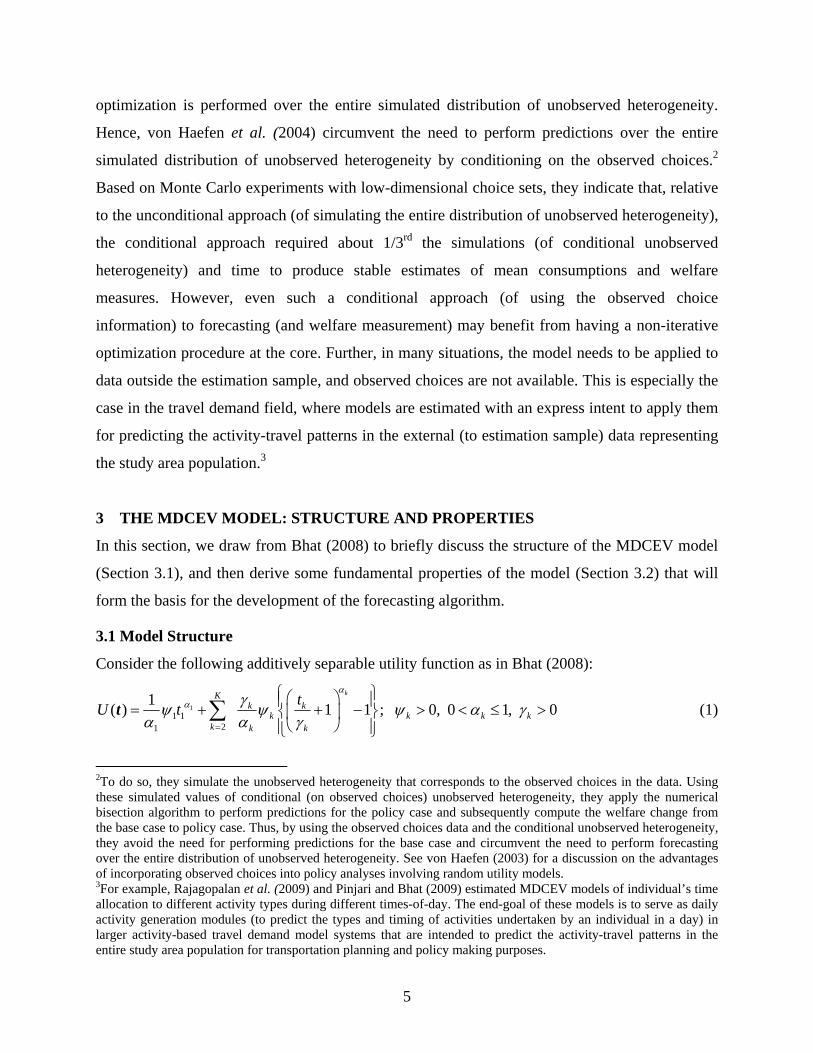
3 THE MDCEV MODEL: STRUCTURE AND PROPERTIES
In this section, we draw from Bhat (2008) to briefly discuss the structure of the MDCEV model
(Section 3.1), and then derive some fundamental properties of the model (Section 3.2) that will
form the basis for the development of the forecasting algorithm.
3.1 Model Structure
Consider the following additively separable utility function as in Bhat (2008):
11 1
21
1( ) 1 1 ; 0, 0 1, 0kK
k kk k k k
k k k
tU tα
α γψ ψ ψ α γα α γ=
⎧ ⎫⎛ ⎞⎪ ⎪= + + − > < ≤ >⎨ ⎬⎜ ⎟⎝ ⎠⎪ ⎪⎩ ⎭
∑t (1)
2To do so, they simulate the unobserved heterogeneity that corresponds to the observed choices in the data. Using these simulated values of conditional (on observed choices) unobserved heterogeneity, they apply the numerical bisection algorithm to perform predictions for the policy case and subsequently compute the welfare change from the base case to policy case. Thus, by using the observed choices data and the conditional unobserved heterogeneity, they avoid the need for performing predictions for the base case and circumvent the need to perform forecasting over the entire distribution of unobserved heterogeneity. See von Haefen (2003) for a discussion on the advantages of incorporating observed choices into policy analyses involving random utility models. 3For example, Rajagopalan et al. (2009) and Pinjari and Bhat (2009) estimated MDCEV models of individual’s time allocation to different activity types during different times-of-day. The end-goal of these models is to serve as daily activity generation modules (to predict the types and timing of activities undertaken by an individual in a day) in larger activity-based travel demand model systems that are intended to predict the activity-travel patterns in the entire study area population for transportation planning and policy making purposes.

6
In the above expression, U(t) is the total utility accrued from consuming t (a Kx1 vector with
non-negative consumption quantities kt ; k = 1,2,…,K) amount of the K alternatives available to
the decision maker. The kψ terms (k = 1,2,…,K), called as the baseline utility parameters,
represents the marginal utility of one unit of consumption of alternative k at the point of zero
consumption for that alternative (Bhat, 2008). Through the kψ terms, the impact of observed and
unobserved alternative attributes, decision-maker attributes, and the choice environment
attributes may be introduced as exp( )k k kzψ β ε′= + , where kz contains the observed attributes
and kε captures the unobserved factors. The kα terms (k = 1,2,…,K), labeled as satiation
parameters (0 1)kα< ≤ , capture satiation effects by reducing the marginal utility accrued from
each unit of additional consumption of alternative k (Bhat, 2008).4 The kγ terms (k = 2,3,…,K),
labeled as translation parameters, play a similar role of satiation as that of kα terms, and an
additional role of translating the indifference curves associated with the utility function to allow
corner solutions (i.e., accommodate the possibility that decision-makers may not consume all
alternatives; see Bhat, 2008). As it can be observed, there is no kγ term for the first alternative
for it is assumed to be an essential Hicksian composite good (or outside good or essential good)
that is always consumed (hence no need for corner solution). Finally, the consumption-based
utility function in (1) can be expressed in terms of expenditures ( ke ) and prices ( kp ) as:5
1
11
21 1
1( ) 1 1 ,kK
k kk
k k k k
eeUp p
ααγψ ψ
α α γ=
⎧ ⎫⎛ ⎞⎛ ⎞ ⎪ ⎪= + + −⎨ ⎬⎜ ⎟⎜ ⎟⎝ ⎠ ⎝ ⎠⎪ ⎪⎩ ⎭
∑e where kk
k
e xp
= (2)
From the analyst’s perspective, the decision-makers maximize the random utility given by
Equation (2) subject to a linear budget constraint and non-negativity constraints on kt :
1(where is the total budget) and 0 ( 1, 2,..., )
K
k k kk
p x E E x k k K=
= ≥ ∀ =∑ (3)
4 Theoretically speaking, the kα values can be negative. But, as indicated by Bhat (2008), imposing the condition
0kα > provides much needed stability in empirical estimations. 5 For the first alternative, 1 1p = , since it is the “numeraire” good. However, in the exposition in the paper, we will
use the notation 1p rather than setting this to 1.

7
The optimal consumptions (or expenditure allocations) can be found by forming the Lagrangian
and applying the Kuhn-Tucker (KT) conditions. The Lagrangian function for the problem is:
L 1
11
2 11 1
1 1 1kK K
k kk k
k kk k k
ee e Ep p
ααγψ ψ λ
α α γ= =
⎧ ⎫⎛ ⎞⎛ ⎞ ⎡ ⎤⎪ ⎪= + + − − −⎨ ⎬⎜ ⎟⎜ ⎟ ⎢ ⎥⎣ ⎦⎝ ⎠ ⎝ ⎠⎪ ⎪⎩ ⎭
∑ ∑ ,
where λ is the Lagrangian multiplier associated with the budget constraint. The KT first-order
conditions for the optimal expenditure allocations *( ; 1, 2,..., )ke k K= are given by:
1 1*1 1
1 1
0ep p
αψ λ
−⎛ ⎞
− =⎜ ⎟⎝ ⎠
, since *1 0e > ,
1*
1 0k
k k
k k k
ep p
αψ λ
γ
−⎛ ⎞
+ − =⎜ ⎟⎝ ⎠
, if * 0,ke > (k = 2,…, K) (4)
1*
1 0k
k k
k k k
ep p
αψ λ
γ
−⎛ ⎞
+ − <⎜ ⎟⎝ ⎠
, if * 0,ke = (k = 2,…, K)
As indicated earlier, these stochastic KT conditions form the basis for model estimation (see
Bhat, 2008). Next, using these same stochastic KT conditions, we derive a few properties of the
MDCEV model that can be exploited to develop a highly efficient forecasting algorithm.
3.2 Model Properties
Property 1: The price-normalized baseline utility of a chosen good is always greater than that of
a good that is not chosen.
ji
i jp pψψ ⎛ ⎞⎛ ⎞
> ⎜ ⎟⎜ ⎟ ⎜ ⎟⎝ ⎠ ⎝ ⎠ if ‘i’ is a chosen good and ‘j’ is not a chosen good. (5)
Proof: The KT conditions in (4) can be rewritten as: 1 1*
1 1
1 1
ep p
αψ λ
−⎛ ⎞
=⎜ ⎟⎝ ⎠
,
1*
1k
k k
k k k
ep p
αψ λ
γ
−⎛ ⎞
+ =⎜ ⎟⎝ ⎠
, if * 0,ke > (k = 2,…, K) (i.e., for all chosen goods) (6)

8
k
kpψ λ< , if * 0,ke = (k = 2,…, K) (i.e., for all goods that are not chosen)
The above KT conditions can further be rewritten as: 11 1* *
*1 1
1 1
1 , if 0, ( 2,3,..., )k
k kk
k k k
e e e k Kp p p p
α αψ ψ
γ
− −⎛ ⎞ ⎛ ⎞ ⎛ ⎞⎛ ⎞
= + > =⎜ ⎟ ⎜ ⎟ ⎜ ⎟⎜ ⎟⎝ ⎠⎝ ⎠⎝ ⎠ ⎝ ⎠
(7)
1 1**1 1
1 1
< , if 0, ( 2,3,..., )kk
k
e e k Kp p p
αψ ψ
−⎛ ⎞ ⎛ ⎞⎛ ⎞
= =⎜ ⎟ ⎜ ⎟⎜ ⎟⎝ ⎠⎝ ⎠⎝ ⎠
Now, consider two alternatives ‘i’ and ‘j’, of which ‘i’ is chosen and ‘j’ is not chosen by a
consumer. For that consumer, the above KT conditions for alternatives ‘i’ and ‘j’ can be written
as: 11 1* *
1 1
1 1
1 , andi
i i
i i i
e ep p p p
α αψ ψ
γ
− −⎛ ⎞ ⎛ ⎞ ⎛ ⎞⎛ ⎞
= +⎜ ⎟ ⎜ ⎟ ⎜ ⎟⎜ ⎟⎝ ⎠⎝ ⎠⎝ ⎠ ⎝ ⎠
(8)
1 1*1 1
1 1
<j
j
ep p p
αψ ψ−⎛ ⎞ ⎛ ⎞⎛ ⎞
⎜ ⎟ ⎜ ⎟⎜ ⎟⎜ ⎟ ⎝ ⎠⎝ ⎠⎝ ⎠
Further, since 1*
1j
j
j j
ep
α
γ
−⎛ ⎞
+⎜ ⎟⎜ ⎟⎝ ⎠
is always greater than 1, one can write the following inequality:
1 111 1** *1 1 1 1
1 1 1 1
< 1i
j i
j i i
ee ep p p p p p
αα αψ ψ ψγ
−− −⎛ ⎞ ⎛ ⎞⎛ ⎞⎛ ⎞ ⎛ ⎞⎛ ⎞< +⎜ ⎟ ⎜ ⎟⎜ ⎟⎜ ⎟ ⎜ ⎟⎜ ⎟⎜ ⎟ ⎝ ⎠⎝ ⎠ ⎝ ⎠⎝ ⎠⎝ ⎠⎝ ⎠
(9)
As one can observe, the third term in the above inequality is nothing but i
ipψ⎛ ⎞⎜ ⎟⎝ ⎠
. Thus, by the
transitive property of inequality of real numbers, the above inequality implies a fundamental
property of the MDCEV model that ji
i jp pψψ ⎛ ⎞⎛ ⎞
> ⎜ ⎟⎜ ⎟ ⎜ ⎟⎝ ⎠ ⎝ ⎠. In words, the price-normalized baseline
utility of a chosen good is always greater than that of a good that is not chosen.
Corollary 1.1: It naturally follows from the property above that when all the K
alternatives/goods available to a consumer are arranged in the descending order of their price-

9
normalized baseline utility values (with the outside good being the first in the order), and if it is
known that the number of chosen alternatives is M, then one can easily identify the chosen
alternatives as the first M alternatives in the arrangement.6
Property 2: The minimum consumption amount of the outside good is
1
11
1
1
(2,3,..., )
.max k
k Kk
p
p
αψ
ψ
−
∀ =
⎛ ⎞⎛ ⎞⎜ ⎟⎜ ⎟
⎝ ⎠⎜ ⎟⎜ ⎟⎛ ⎞⎜ ⎟⎜ ⎟⎜ ⎟⎝ ⎠⎝ ⎠
Proof: Using the first and third KT conditions in (6), and considering market baskets that involve
only the consumption of the outside good (i.e., * 0, 1)ke k= ∀ > . At these market baskets, one can
write the following: 1 1*
1 1
1 1
; (2,3,..., ),k
k
e k Kp p p
αψ ψ
−⎛ ⎞ ⎛ ⎞
< ∀ =⎜ ⎟ ⎜ ⎟⎝ ⎠⎝ ⎠
or, 1 1*
1 1
(2,3,..., )1 1
max .k
k Kk
ep p p
αψ ψ
−
∀ =
⎛ ⎞ ⎛ ⎞<⎜ ⎟ ⎜ ⎟
⎝ ⎠⎝ ⎠
Hence,
1
11
1*
11
1
(2,3,..., )
.max k
k Kk
pep
p
αψ
ψ
−
∀ =
⎛ ⎞⎛ ⎞⎜ ⎟⎜ ⎟⎛ ⎞ ⎝ ⎠⎜ ⎟>⎜ ⎟ ⎜ ⎟⎛ ⎞⎝ ⎠ ⎜ ⎟⎜ ⎟⎜ ⎟⎝ ⎠⎝ ⎠
(10)
In words, the right side of the above equation represents the “minimum” amount of
consumption of the outside good. The interpretation is that, after the “minimum” amount of
outside good is consumed, all other goods (and the outside good) start competing for the
remaining amount of the budget. Thus, if the budget amount is less than that corresponding to the
minimum consumption of outside good given in (10), no other goods will be consumed. Another
interesting point to note here is that if there is no price variation across the consumption
alternatives, the distribution of the minimum consumption of the outside good can be derived as
a log-logistic variable.
6The reader is cautioned to note here that the converse of this property may not always hold true. That is, given the price-normalized utilities of two alternatives, one can not say with certanity if one (with higher value of price-normalized utility) or both of the alternatives are chosen.

10
Property 3: When all the satiation parameters ( )kα are equal, and if the corner solutions are
known (i.e., if the chosen and not-chosen alternatives are known), the Lagrange multiplier of the
utility maximization as well as the optimal consumptions of the chosen goods can be expressed in
an analytical form.
Proof:7 Using the first and second KT conditions in (6), and assuming without loss of generality
that the first M goods are chosen, one can express the optimal consumptions as:
1
1* 11 1
1 1
1* 1
, and
1 ; (2,3,..., )k
k kk
k k
e pp
e p k Mp
α
α
λψ
λ γψ
−
−
⎛ ⎞= ⎜ ⎟⎝ ⎠⎧ ⎫⎛ ⎞⎪ ⎪= − ∀ =⎨ ⎬⎜ ⎟⎝ ⎠⎪ ⎪⎩ ⎭
(11)
Using these expressions, the budget constraint in (3) can be written as:
1
1111
11
21
1kM
kk k
k k
ppp p Eαα
λ λ γψ ψ
−−
=
⎧ ⎫⎛ ⎞⎛ ⎞ ⎪ ⎪+ − =⎨ ⎬⎜ ⎟⎜ ⎟
⎝ ⎠ ⎝ ⎠⎪ ⎪⎩ ⎭∑
From the above equation, and assuming that all satiation ( )kα parameters as equal to α , the
Lagrange multiplierλ can be expressed analytically as: 1
211
111
121
M
k kk
Mk
k kk k
E p
p pp p
α
αα
γλ
ψψ γ
−
=
−−
=
⎛ ⎞⎜ ⎟+⎜ ⎟
= ⎜ ⎟⎜ ⎟⎛ ⎞⎛ ⎞⎜ ⎟+ ⎜ ⎟⎜ ⎟⎜ ⎟⎝ ⎠ ⎝ ⎠⎝ ⎠
∑
∑ (12)8
The above expression for λ can be substituted back into the expressions in (11) to obtain the
following analytical expressions for optimal consumptions:
7To be sure, this is a standard property and has been proved elsewhere, albeit with different functional forms. Nonetheless, we provide a proof here for completeness. 8 The reader will note here that this expression contains terms corresponding to the consumed goods only.
11
11
1*
21111
1 111
121
M
k kk
Mk
k kk k
E ppe
pp p
p p
α
αα
ψ γ
ψψ γ
−
=
−−
=
⎛ ⎞ ⎛ ⎞+⎜ ⎟ ⎜ ⎟
⎝ ⎠⎝ ⎠=⎛ ⎞⎛ ⎞
+ ⎜ ⎟⎜ ⎟⎝ ⎠ ⎝ ⎠
∑
∑ (13)
11
*2
1111
11
21
1 ; (2,3,..., )
Mk
k kkkk
kMk
kk k
k k
E ppe k M
pp p
p p
α
αα
ψ γγ
ψψ γ
−
=
−−
=
⎛ ⎞⎛ ⎞ ⎛ ⎞⎜ ⎟+⎜ ⎟ ⎜ ⎟⎜ ⎟⎝ ⎠⎝ ⎠= − ∀ =⎜ ⎟
⎜ ⎟⎛ ⎞⎛ ⎞⎜ ⎟+ ⎜ ⎟⎜ ⎟⎜ ⎟⎝ ⎠ ⎝ ⎠⎝ ⎠
∑
∑. (14)
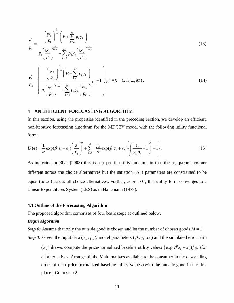
4 AN EFFICIENT FORECASTING ALGORITHM
In this section, using the properties identified in the preceding section, we develop an efficient,
non-iterative forecasting algorithm for the MDCEV model with the following utility functional
form:
11 1
21
1( ) exp( ) exp( ) 1 1 ,K
k kk k
k k k
eeU z zp p
ααγβ ε β ε
α α γ=
⎧ ⎫⎛ ⎞⎛ ⎞ ⎪ ⎪′ ′= + + + + −⎨ ⎬⎜ ⎟⎜ ⎟⎝ ⎠ ⎝ ⎠⎪ ⎪⎩ ⎭
∑e (15)
As indicated in Bhat (2008) this is a -profileγ utility function in that the kγ parameters are
different across the choice alternatives but the satiation ( kα ) parameters are constrained to be
equal (to α ) across all choice alternatives. Further, as 0α → , this utility form converges to a
Linear Expenditures System (LES) as in Hanemann (1978).
4.1 Outline of the Forecasting Algorithm
The proposed algorithm comprises of four basic steps as outlined below.
Begin Algorithm
Step 0: Assume that only the outside good is chosen and let the number of chosen goods M = 1.
Step 1: Given the input data ( kz , kp ), model parameters (β , kγ ,α ) and the simulated error term
( kε ) draws, compute the price-normalized baseline utility values ( )exp( )k k kz pβ ε′ + for
all alternatives. Arrange all the K alternatives available to the consumer in the descending
order of their price-normalized baseline utility values (with the outside good in the first
place). Go to step 2.
12
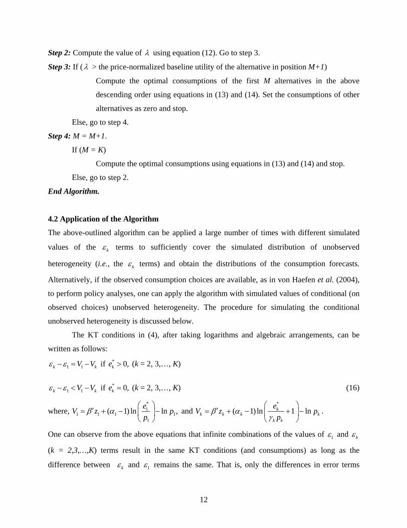
Step 2: Compute the value of λ using equation (12). Go to step 3.
Step 3: If (λ > the price-normalized baseline utility of the alternative in position M+1)
Compute the optimal consumptions of the first M alternatives in the above
descending order using equations in (13) and (14). Set the consumptions of other
alternatives as zero and stop.
Else, go to step 4.
Step 4: M = M+1.
If (M = K)
Compute the optimal consumptions using equations in (13) and (14) and stop.
Else, go to step 2.
End Algorithm.
4.2 Application of the Algorithm
The above-outlined algorithm can be applied a large number of times with different simulated
values of the kε terms to sufficiently cover the simulated distribution of unobserved
heterogeneity (i.e., the kε terms) and obtain the distributions of the consumption forecasts.
Alternatively, if the observed consumption choices are available, as in von Haefen et al. (2004),
to perform policy analyses, one can apply the algorithm with simulated values of conditional (on
observed choices) unobserved heterogeneity. The procedure for simulating the conditional
unobserved heterogeneity is discussed below.
The KT conditions in (4), after taking logarithms and algebraic arrangements, can be
written as follows:
1 1k kV Vε ε− = − if * 0,ke > (k = 2, 3,…, K)
1 1k kV Vε ε− < − if * 0,ke = (k = 2, 3,…, K) (16)
where, *1
1 1 1 11
( 1) ln ln ,eV z pp
β α⎛ ⎞
′= + − −⎜ ⎟⎝ ⎠
and *
( 1) ln 1 lnkk k k k
k k
eV z pp
β αγ
⎛ ⎞′= + − + −⎜ ⎟
⎝ ⎠.
One can observe from the above equations that infinite combinations of the values of 1ε and kε
(k = 2,3,…,K) terms result in the same KT conditions (and consumptions) as long as the
difference between kε and 1ε remains the same. That is, only the differences in error terms

13
matter (Bhat, 2008). Based on this insight, one can recast the MDCEV model with a differenced-
error structure where the outside good is associated with no error term and the remaining K-1
goods are associated with a multivariate logistic distributed error structure
(i.e., ,1 1; 2,3,...,k k k Kε ε ε= − = ; see Appendix C of Bhat, 2008 for more details). Thus, it is
sufficient to simulate the differences in error terms ( ,1 1k kε ε ε= − ) rather than the error terms
( 1 and kε ε ) themselves. Based on this insight, one can assume that the differenced-error term for
the outside good is zero (i.e., 1,1 1 1 0ε ε ε= − = ) and simulate the differenced-unobserved error
terms for other alternatives. For chosen alternatives, one can easily do so by using the first
equation in (16) (i.e., ,1 1k kV Vε = − ). To simulate the differenced-error terms for the not-chosen
alternatives, the analyst has to draw from a truncated multivariate logistic distribution resulting
from the second equation in (16).9
4.3 Intuitive Interpretation of the Algorithm
As it can be observed, the proposed algorithm in Section 4.1 builds on the insight from corollary
1.1 that if the number of chosen alternatives is known, one can easily identify the chosen
alternatives by arranging the price-normalized baseline utility values in a descending order.
Subsequently, one can compute the optimal consumptions of the chosen alternatives using
Equations (13) and (14). The only issue, however, is that the number of chosen alternatives is
unknown apriori. To find this out, the algorithm begins with an assumption that only one
alternative (i.e., the outside good) is chosen and verifies this assumption by verifying the KT
conditions (i.e., the condition in Step 3) for other, (assumed to be)not-chosen goods. If the KT
conditions (i.e., the condition in Step 3) are met, the algorithm stops. Else, at least the next
alternative (in the order of the price-normalized baseline utilities) has to be among the chosen
alternatives. Thus, the KT conditions (i.e., the condition in step 3) are verified again by assuming
that the next alternative is among the chosen alternatives. These basic steps are repeated until
either the KT conditions (i.e., the condition in step 3) are met or the assumed number of chosen
alternatives reaches the maximum number (K).
9 The reader will note here that the procedure to simulate the conditional (on observed choices) error terms described here for the MDCEV model is different from that in von Haefen et al. (2004), due to the subtle (but important) differences in the assumptions on stochasticity between the MDCEV and von Haefen et al. models (see Bhat, 2008).
14
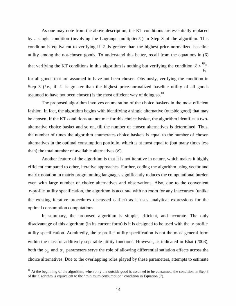
As one may note from the above description, the KT conditions are essentially replaced
by a single condition (involving the Lagrange multiplierλ ) in Step 3 of the algorithm. This
condition is equivalent to verifying if λ is greater than the highest price-normalized baseline
utility among the not-chosen goods. To understand this better, recall from the equations in (6)
that verifying the KT conditions in this algorithm is nothing but verifying the condition k
kpψλ >
for all goods that are assumed to have not been chosen. Obviously, verifying the condition in
Step 3 (i.e., if λ is greater than the highest price-normalized baseline utility of all goods
assumed to have not been chosen) is the most efficient way of doing so.10
The proposed algorithm involves enumeration of the choice baskets in the most efficient
fashion. In fact, the algorithm begins with identifying a single alternative (outside good) that may
be chosen. If the KT conditions are not met for this choice basket, the algorithm identifies a two-
alternative choice basket and so on, till the number of chosen alternatives is determined. Thus,
the number of times the algorithm enumerates choice baskets is equal to the number of chosen
alternatives in the optimal consumption portfolio, which is at most equal to (but many times less
than) the total number of available alternatives (K).
Another feature of the algorithm is that it is not iterative in nature, which makes it highly
efficient compared to other, iterative approaches. Further, coding the algorithm using vector and
matrix notation in matrix programming languages significantly reduces the computational burden
even with large number of choice alternatives and observations. Also, due to the convenient
-profileγ utility specification, the algorithm is accurate with no room for any inaccuracy (unlike
the existing iterative procedures discussed earlier) as it uses analytical expressions for the
optimal consumption computations.
In summary, the proposed algorithm is simple, efficient, and accurate. The only
disadvantage of this algorithm (in its current form) is it is designed to be used with the -profileγ
utility specification. Admittedly, the -profileγ utility specification is not the most general form
within the class of additively separable utility functions. However, as indicated in Bhat (2008),
both the kγ and kα parameters serve the role of allowing differential satiation effects across the
choice alternatives. Due to the overlapping roles played by these parameters, attempts to estimate 10 At the beginning of the algorithm, when only the outside good is assumed to be consumed, the condition in Step 3 of the algorithm is equivalent to the “minimum consumption” condition in Equation (7).

15
utility functions that allow both the kγ and kα parameters to vary across alternatives may lead to
severe empirical identification issues and estimation breakdowns. Further, “for a given kψ value,
it is possible to closely approximate a sub-utility function based on a combination of kγ and kα
values with a sub-utility function solely based on kγ or kα values” (Bhat, 2008). For these
reasons, and given the ease of forecasting with the proposed algorithm (see Section 4.4), we
suggest an estimation of the -profileγ utility function. Nevertheless, the insights obtained from
the properties 1 and 2 discussed in the preceding section (and parts of this algorithm) can be used
to design an efficient (albeit iterative) algorithm for cases when kα parameters vary across
alternatives. For example, the numerical bisection algorithm of von Haefen et al., which can be
used for forecasting with the MDCEV model when kα parameters vary, can potentially be made
more efficient based on the insights obtained from properties 1 and 2.
4.4 Generalization of the Forecasting Algorithm for other KT Demand Model Systems
The algorithm developed in Section 4.1 is tailored to the MDCEV model. However, similar
properties as in Section 3 can be derived, and similar forecasting algorithms can be developed for
other KT demand model systems in the literature. Specifically, the basic algorithmic approach
remains the same as that in Section 4.1, except that steps 1, 2, and 3 of the algorithm vary
slightly depending on the form of the utility function employed in different KT demand systems.
Specifically, the following modifications will be needed for a different form of utility function:
• In step 1, all the K available alternatives have to be arranged in the descending order based
on a measure that depends on the form of the utility function (with the outside good being the
first in the order). Such a measure can be easily derived for different forms of utility
functions used in the literature by following the derivations of the proof of property 1 in
Section 3.1. For the MDCEV model, as shown in Section 3.1, this measure is the price-
normalized baseline utility. That is, for the MDCEV model, the alternatives have to be
arranged in the descending order of their price-normalized baseline utility values.11
11This discussion suggests a general property of the KT demand system models used in the literature so far (with additive utility functions) that the choice alternatives can always be arranged in the descending order of a specific measure that depends on the form of the utility function. The generality of this property and the conditions under which such a measure may not exist is yet to be thoroughly investigated.

16
• In step 2, the formula for the computation of the Lagrange multiplier (λ ) will depend on the
form of the utility function. The analytical formula for λ can be derived following the proof
of property 3 in Section 3.1, as long as the kα parameters do not vary across different
alternatives.
• In step 3, the Lagrange multiplier (λ ) will have to be compared with the same measure that
was used to arrange the K alternatives in the descending order. The formulae for the optimal
consumptions (conditional on the knowledge of the consumed alternatives) will also depend
on the form of the utility function. Again, these formulae can also be derived in a straight
forward fashion for utility functions with same kα parameter across all alternatives.
Thus, the proposed algorithm is fairly generic in its approach, and can be easily modified to be
used with different forms of utility functions.
4.5 Application Results
Limited experiments were conducted to assess the performance of the algorithm. Specifically,
the performance of the proposed algorithm and that of a traditionally used iterative optimization
routine were compared. Empirical data on household transportation expenditures, obtained from
the 2002 Consumer Expenditure Survey conducted by the Bureau of Labor Statistics (BLS,
2003), available at the National Bureau of Economic Research data archives (NBER, 2003), was
used for the experiments. This data was extracted by Ferdous et al. (2009) and used in Pinjari
(2009) to analyze household expenditures in six transportation categories (or alternatives),
including: (1) Vehicle purchases, (2) Gasoline and motor oil, (3) Vehicle insurance, (4) Vehicle
maintenance, (5) Air travel, and (6) Public transportation, and a seventh, outside category that
includes all other expenditures of a household. An MDCEV model with these seven expenditure
alternatives was estimated using data from 4000 households. These model parameters and the
data of the 4000 households were used for subsequent experiments.
The proposed algorithm was coded and executed in Gauss matrix programming language.
In addition, for comparison purposes, the iterative constrained optimization routines of the
Constrained Maximum Likelihood (CML) module of Gauss were also used for forecasting the
household expenditures in the empirical data. The CML module of Gauss uses a sequential
programming method for carrying out non-linear optimization, in which the optimal
consumption values are approximated iteratively using the first and second gradients of the
17
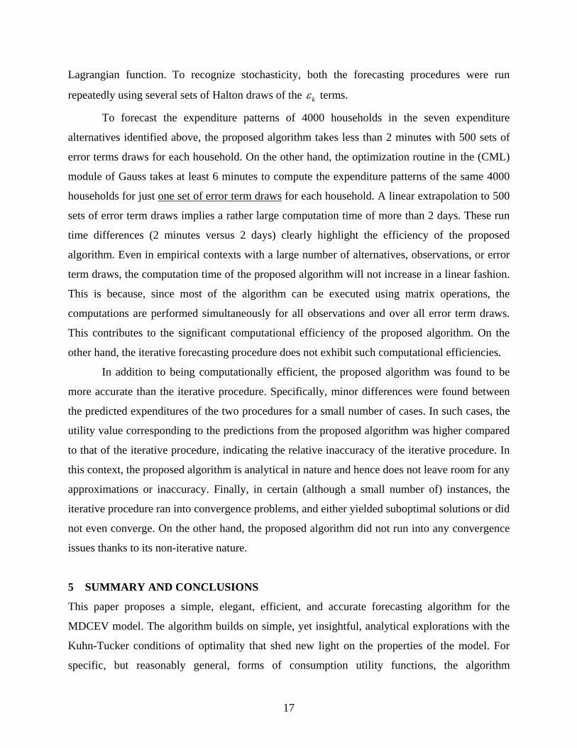
Lagrangian function. To recognize stochasticity, both the forecasting procedures were run
repeatedly using several sets of Halton draws of the kε terms.
To forecast the expenditure patterns of 4000 households in the seven expenditure
alternatives identified above, the proposed algorithm takes less than 2 minutes with 500 sets of
error terms draws for each household. On the other hand, the optimization routine in the (CML)
module of Gauss takes at least 6 minutes to compute the expenditure patterns of the same 4000
households for just one set of error term draws for each household. A linear extrapolation to 500
sets of error term draws implies a rather large computation time of more than 2 days. These run
time differences (2 minutes versus 2 days) clearly highlight the efficiency of the proposed
algorithm. Even in empirical contexts with a large number of alternatives, observations, or error
term draws, the computation time of the proposed algorithm will not increase in a linear fashion.
This is because, since most of the algorithm can be executed using matrix operations, the
computations are performed simultaneously for all observations and over all error term draws.
This contributes to the significant computational efficiency of the proposed algorithm. On the
other hand, the iterative forecasting procedure does not exhibit such computational efficiencies.
In addition to being computationally efficient, the proposed algorithm was found to be
more accurate than the iterative procedure. Specifically, minor differences were found between
the predicted expenditures of the two procedures for a small number of cases. In such cases, the
utility value corresponding to the predictions from the proposed algorithm was higher compared
to that of the iterative procedure, indicating the relative inaccuracy of the iterative procedure. In
this context, the proposed algorithm is analytical in nature and hence does not leave room for any
approximations or inaccuracy. Finally, in certain (although a small number of) instances, the
iterative procedure ran into convergence problems, and either yielded suboptimal solutions or did
not even converge. On the other hand, the proposed algorithm did not run into any convergence
issues thanks to its non-iterative nature.
5 SUMMARY AND CONCLUSIONS
This paper proposes a simple, elegant, efficient, and accurate forecasting algorithm for the
MDCEV model. The algorithm builds on simple, yet insightful, analytical explorations with the
Kuhn-Tucker conditions of optimality that shed new light on the properties of the model. For
specific, but reasonably general, forms of consumption utility functions, the algorithm

18
circumvents the need to carry out any iterative constrained optimization procedures that have
hitherto been used for forecasting with Kuhn-Tucker (KT) demand system models. The non-
iterative nature of the algorithm contributes significantly to its efficiency and accuracy. Further,
although developed in the context of the MDCEV model, the proposed algorithm can be easily
modified to be used in the context of other utility maximization-based Kuhn-Tucker (KT)
consumer demand model systems in the literature.
Results from the application of the proposed algorithm and a traditionally used iterative
algorithm indicate the significant computational efficiency (as well as accuracy) of the proposed
algorithm. The appealing feature of the algorithm is that most of it can be in executed using
matrix operations, which enable a simultaneous computation for a large number of observations
and huge computational efficiencies.
As the proposed algorithm makes it easier to perform forecasting and policy analysis with
MDCEV and other KT demand model systems, it is hoped that these types of models will soon
be utilized for practical transportation planning and policy analysis purposes. Further, now that a
fast and easy-to-use forecasting procedure is available, further research can be conducted to
characterize the distributions of forecasts obtained from MDCEV and other KT demand model
systems.
ACKNOWLEDGEMENTS
This research was supported partially by a faculty start-up grant to the first author from the
University of South Florida.

19
REFERENCES
Ahn, J., Jeong, G., and K. Yeonbae (2007) A forecast of household ownership and use of alternative fuel vehicles: A multiple discrete-continuous choice approach. Energy Economics, 30(5), 2091-2104.
Bhat, C.R. (2005) A Multiple Discrete-Continuous Extreme Value Model: Formulation and Application to Discretionary Time-Use Decisions. Transportation Research-B, 39(8) 679-707.
Bhat, C.R. (2008) The Multiple Discrete-Continuous Extreme Value (MDCEV) Model: Role of Utility Function Parameters, Identification Considerations, and Model Extensions. Transportation Research-B, 42(3), 274-303.
Bhat, C.R., S. Sen, and N. Eluru (2008). The Impact of Demographics, Built Environment Attributes, Vehicle Characteristics, and Gasoline Prices on Household Vehicle Holdings and Use. Transportation Research-B, 43(1) 1-18.
BLS (2003) 2002 Consumer Expenditure Interview Survey Public Use Microdata Documentation. U.S. Department of Labor Bureau of Labor Statistics, Washington, D.C.
Fang, H.A. (2008). A discrete–continuous model of households’ vehicle choice and usage, with an application to the effects of residential density. Forthcoming in Transportation Research Part B 42(9), 736-758.
Ferdous, N., Pinjari A.R., Bhat C.R., and R.M. Pendyala (2008). A Comprehensive Analysis of Household Expenditures in the United States: Evidence from the 2002 Consumer Expenditure Survey Data. Technical Paper, The University of Texas at Austin.
Habib, K. M. N., Miller, E. J. (2009) Modeling Activity Generation: A Utility-based Model for Activity Agenda Formation. Transportmetrica 5(1), 3-23.
Hanemann, W.M., 1978. A methodological and empirical study of the recreation benefits from water quality improvement. Ph.D. dissertation, Department of Economics, Harvard University.
Kim, J., G.M. Allenby, and P.E. Rossi (2002). Modeling consumer demand for variety. Marketing Science, 21, 229-250.
NBER (1980-2003) The National Bureau of Economic Research (NBER) Archive of Consumer Expenditure Survey Microdata Extracts. http://www.nber.org/data/ces_cbo.html.
Phaneuf, D.J., Kling, C.L., and Herriges, J.A., 2000. Estimation and welfare calculations in a generalized corner solution model with an application to recreation demand. The Review of Economics and Statistics, 82(1), 83-92.
Pinjari, A.R., Bhat, C.R., and Hensher, D.A. (2009) Residential Self-Selection Effects in an Activity Time-use Behavior Model. Transportation Research Part B, 43(7), 729-748.
Pinjari, A.R. (2009) Generalized Extreme Value (GEV)-based Error Structures for Multiple Discrete-Continuous Choice Models. Technical Paper. Department of Civil and Environmental Engineering, University of South Florida.
20
Pinjari, A.R., and C.R. Bhat (2009) A Multiple Discrete-Continuous Nested Extreme Value Model: Formulation and Application to Non-Worker Activity Time-use and Timing Behavior on Weekdays. Accepted, Transportation Research Part B.
Rajagopalan, B.S., and K.S., Srinivasan (2008) Integrating Household-Level Mode Choice and Modal Expenditure Decisions in a Developing Country: Multiple Discrete-Continuous Extreme Value Model. Transportation Research Record, No. 2076, 41-51.
Rajagopalan, B.S., Pinjari, A.R., and C.R. Bhat (2008) A Comprehensive Model of Worker’s Non-work Activity Time-use and Timing Behavior. Forthcoming, Transportation Research Record.
Srinivasan, S., and C.R. Bhat (2006). A Multiple Discrete-Continuous Model for Independent- and Joint- Discretionary-Activity Participation Decisions. Transportation, 33 (5), 497-515.
Vasquez-Lavin, F., and M. Hanemann (2009) Functional Forms in Discrete/Continuous Choice Models with General Corner Solutions. Proceedings of the 1st International Choice Modeling Conference, Harrogate, March 2009.
von Haefen, R.H. (2003) Incorporating observed choice into the construction of welfare measures from random utility models. Journal of Environmental Economics & Management, 45(2), 145-165.
von Haefen, R.H., Phaneuf, D.J., and Parsons, G.R. (2004) Estimation and welfare analysis with large demand systems. Journal of Business and Economic Statistics, 22(2), 194-205.
von Haefen, R.H., and D.J. Phaneuf (2005) Kuhn-Tucker Demand System Approaches to Nonmarket Valuation, in R. Scarpa and A.A. Alberini (Eds.), Applications of Simulation Methods in Environmental and Resource Economics, Springer.
Wales, T.J., and Woodland, A.D. (1983) Estimation of Consumer Demand Systems with Binding Non-Negativity Constraints. Journal of Econometrics, 21(3), 263-85.