An Edgeworth Series Expansion forMultipath Fading Channel Densities

Nickie Menemenlis C. D. Charalambous

McGill University University of Ottawa

41st IEEE 2002 Conference on Decision and ControlDecember 10 - 13, 2002

Las Vegas, Nevada

Overview

Wireless Communication System

Channel output viewed as a shot-noise process

Double-stochastic Poisson process with fixed realization of its rate

Characteristic and moment generating functions

Central-limit theorem

Edgeworth series of received signal density

Wireless Communication Propagation Channels

Area 2Area 1

Transmitter

Log-normalshadowing

Short-term fading

Shannon’s Wireless Communication System

SourceSource

EncoderChannelEncoder

Mod-ulator

UserSource

DecoderChannelDecoder

Demod-ulator

MessageSignal

Channel code word

Estimate ofMessage

signalEstimate of

channel code word

ReceivedSignal

ModulatedTransmitted

Signal

Wireless

Channel

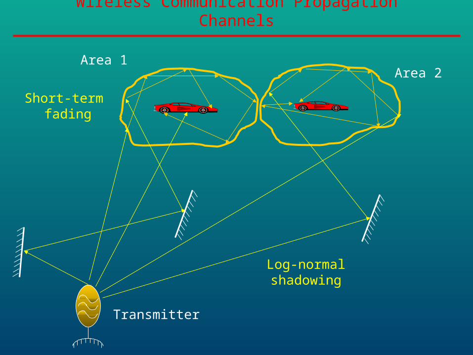
Impulse Response Characterization

(t0)t0

t2

(t2)

t1(t1)

Time spreading property

Time va

riatio

ns property

Impulse response: Time-spreading : multipath

and time-variations: time-varying environment

Impulse Response Multipath Fading Channel

( )( ; )

1

( )( ; )

1

Response of the channel at time due an impulse

applied at time - .

( ; ) ( ; ) ( ( ))

( ; ) Re ( ; ) ( ( ))

( ; ): Signal attenuation (R.P.

i

i c

N tj t

l i ii

N tj t j t

i ii

i

t

t

C t r t e t t

C t r t e e t t

r t

)

( ; ) ( ) : Phase angle (R.P.)

( ) : Propagation delay (R.P.)

( ): Number of waves impinging on the receiver

antenna at time (a counting R.P.)

i ii i c d d

i

t t

t

N t

t

Band-pass representation of impulse response:

Band-pass Representation of Impulse Response

( )( ; )

1

( )

1

( ; ) Re ( ; ) ( ( ))

( ; ) cos ( ; )sin ( ( ))

( ; ) ( ; ) cos( ( ; )) In-phase component

( ; ) ( ; )sin( ( ; )) Quadr

i c

N tj t j t

i ii

N t

i c i c ii

i i i

i i i

C t r t e e t t

I t t Q t t t t

I t r t t

Q t r t t

2 2

1

ature component

( ; ) ( ; ) ( ; ) Attenuation

( ; )( ; ) tan Phase( ; )

ii i

ii

i

r t I t Q t

Q tt I t

Shot-Noise Channel Model

( )( ; ( ))

1

( )

1

Low pass representation of received signal

( ) ( ; ( )) ( ( ))

Band pass representation of received signal

( ) ( ; ( )) cos ( ; ( )) ( ( ))

( ; ) Pha

s

i i

s

N Tj t t

l i i l ii

N T

i i c i i l ii

i

y t r t t e s t t

y t r t t t t t s t t

t

se shift

( ; ): signal attenuation coefficient, i.e. Rayleigh, Ricean

( ), ( ) : time delays and number of paths

( ; ), ( ; ), ( ) arbitrary random processes

( ) : arbitrary low-pass

i

i

i i i

l

r t

t N t

r t t t

s t

transmitted signal

Channel viewed as a shot-noise effect [Rice 1944]

Shot-Noise Effect

ti ti

Counting process ResponseLinear

system

Shot-Noise Process: Superposition of i.i.d. impulse responses occuring at times obeying a counting process, N(t).

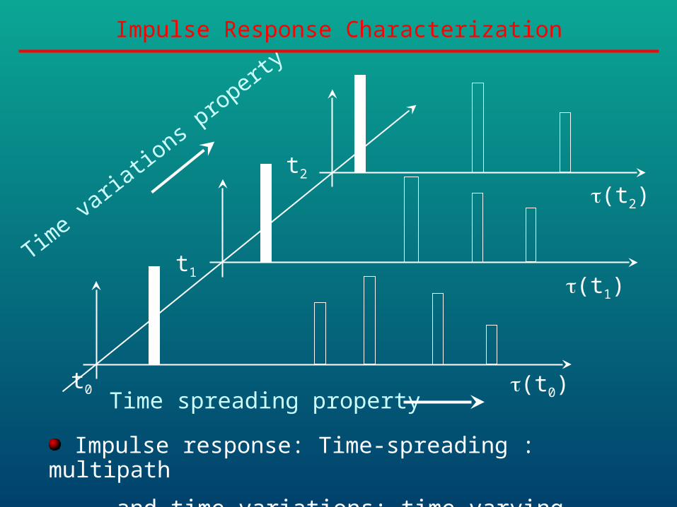
Measured power delay profile

Shot-Noise Effect

Channel Simulations Experimental Data (Pahlavan p. 52)

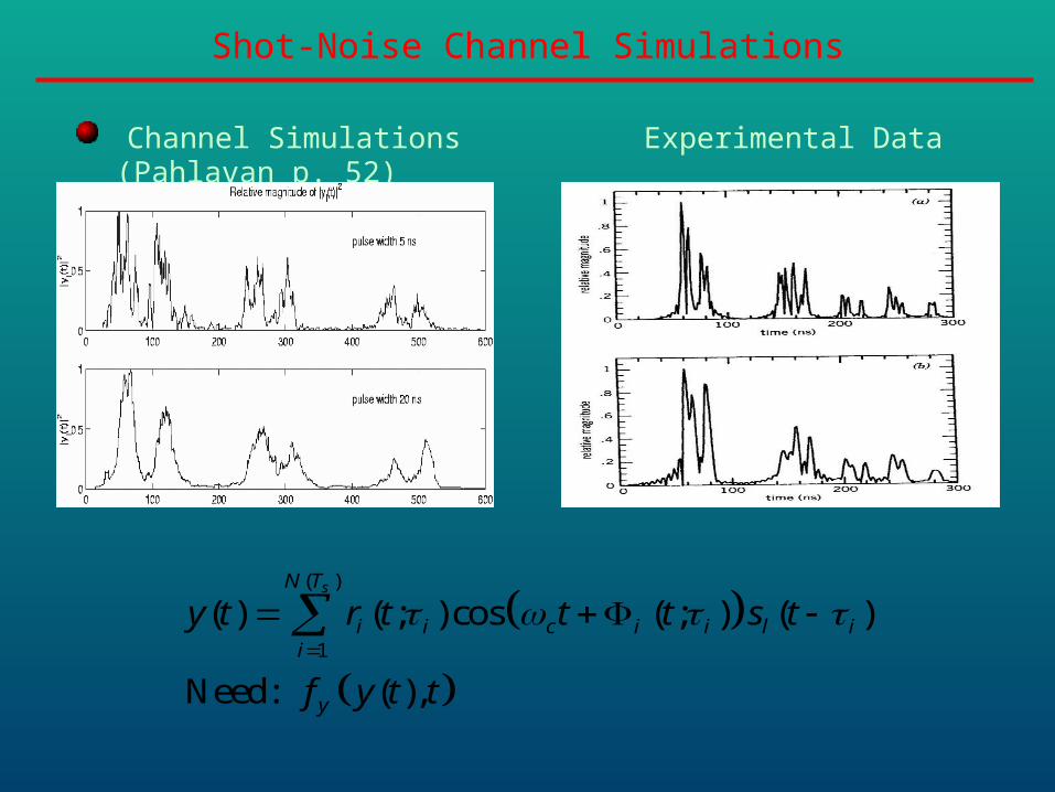
Shot-Noise Channel Simulations

( )

1

( ) ( ; ) cos ( ; ) ( )

Need: ( ),

sN T

i i c i i l ii

y

y t r t t t s t

f y t t

Shot noise processess and Campbell’s theorem

Shot-Noise Definition

( )

1

A stochastic process ( ), , , is said to be a

- if it can be represented as the

superposition of impulses occuring at random times

( ) ( , ;m ( , ))

where occur ac

i

N t

m m m mm

i

X t t

shot noise process

X t h t t

cording to a counting process, ( )

i.e. a non-homogeneous Poisson process, with intensity ( ),

and ( , ;m ( , )) assumed to be independent and

identically distributed random processes, independentm m m m

N t

t

h t t

0

of

( ) .t

N t

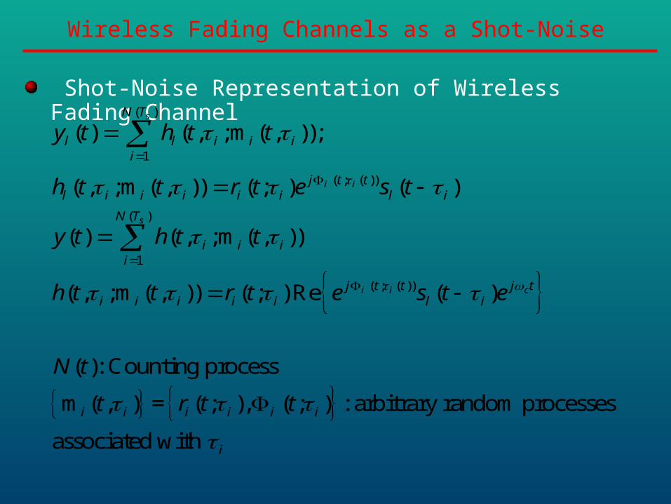
Shot-Noise Representation of Wireless Fading Channel

Wireless Fading Channels as a Shot-Noise

( )

1

( ; ( ))

( )

1

( ; ( ))

( ) ( , ;m ( , ));

( , ;m ( , )) ( ; ) ( )

( ) ( , ;m ( , ))

( , ;m ( , )) ( ; ) Re ( )

( ): Counting process

m ( , ) = ( ;

s

i i

s

i i c

N T

l l i i ii

j t tl i i i i i l i

N T

i i ii

j t t j ti i i i i l i

i i i

y t h t t

h t t r t e s t

y t h t t

h t t r t e s t e

N t

t r t

), ( ; ) : arbitrary random processes

associated with

i i i

i

t

Counting process N(t): Doubly-Stochastic Poisson Process with random rate

Shot-Noise Assumption

0

0

0

22

0 0

Conditional on ( );0 ,

( ) has a Poisson law

( )( ) exp ( )

!

( ) ( ) ,

( ) ( ) ( ) ,

s

s

S

s

S

s

S s

s

T s

s

kT

T

s T

T

s T

T T

s T

s s T

N T

t dtProb N T k t dt

k

N T k t dt

N T k t dt t dt

E

E

Conditional Joint Characteristic Functional of y(t)

Joint Characteristic Function

y 1 1

m0

1

m0

1 1

, ; ; , exp y(t)

exp ( ) exp h t, ;m t, 1

, ln exp (t) ( )!

( ) ( ) , ;m ,

y(t) ( ), , ( ) , , , ,

h t, ;m t

s

s

s

s

n n T

T

k

y T kk

kT

k

n nn n

j t j t E j

E j d

jj t E j y t

k

t E h t t d

y t y t

1 1, , ; , , , , ; ,n nh t m t h t m t

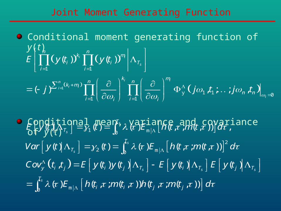
Conditional moment generating function of y(t)

Conditional mean, variance and covariance of y(t)

Joint Moment Generating Function

1

1 1

y 1 1 01 1

1 m0

2

2 m0

( ) ( )

( ) , ; ; ,

( ) ( ) ( ) ( , ; ( , )) ,

( ) ( ) ( ) ( , ; ( , ))

i i

s

i ini ii

i

s

s

s

s

n nk m

i i Ti i

k mn n

k m

n ni ii i

T

T

T

T

E y t y t

j j t j t

E y t t E h t m t d

Var y t t E h t m t d

m0

, ( ) ( ) ( ) ( )

( ) ( , ; ( , )) ( , ; ( , ))

s s s

s

y i j i j T i T j T

T

i i j j

Cov t t E y t y t E y t E y t

E h t m t h t m t d

Conditional Joint Characteristic Functional of yl(t)

Joint Characteristic Function

†

†y 1 1

Re h t, ;m t,

m0

,*

1

*, m0

1 1

, ; ; , exp Re y (t)

exp ( ) 1

( ), ln exp Re (t)

!

( ) ( ) Re , ;m ,

y (t) ( ), , ( ) , ,

l s

s l

l s

s

n n l T

T j

l kky l T

k

kT

l k l

nl l l n

t t E j

E e d

tt E j y j

k

t E h t t d

y t y t

1 1

, ,

h t, ;m t, , ; , , , , ; ,

nn

l l l n nh t m t h t m t

Joint Moment Generating Function

1

1 1

y 1 1 01 1

,1

,22 2

( ) ( )

( 2 ) , ; ; ,

( ) ( 2 ) ( ),

( )( ) ( 2 )

2!

1

2

i i

l s

iini ii

li

i

s

s

i

n nk m

i l i Ti i

mkn n

k m

n ni ii

l T l

ll T

i R

E y t y t

j t t

E y t j j t

tVar y t j j

j

1

; 2

i i i iI R I

j

Conditional moment generating function of yl(t)

Conditional mean and variance of yl(t)

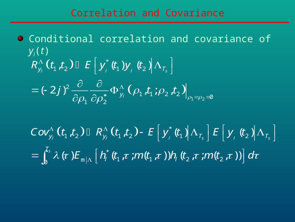
Conditional correlation and covariance of yl(t)

Correlation and Covariance

1 2

*1 2 1 2

21 1 2 2 0

1 2

*1 2 1 2 1 2

*1 1 2 2m0

, ( ) ( )

( 2 ) , ; ,

, , ( ) ( )

( ) ( , ; ( , )) ( , ; ( , ))

l l l s

l

l l l s l s

s

y T

y

y y T T

T

l l

R t t E y t y t

j t t

Cov t t R t t E y t E y t

E h t m t h t m t d

Central Limit Theorem

yc(t) is a multi-dimensional zero-mean Gaussian process with covariance function identified

Central-Limit Theorem

y 1 1

2

m01

Let ( , ) ( , ), where is deterministic

( ) ( )and define ( ) then

( )

lim , ; ; ,

exp ( )2

( , ;m( , ))( )

s

cd

s

d c d

i i T

c iy i

n n

nTd i

li y

ic ii

h

t t

y t E y ty t

t

t t

E dt

t t

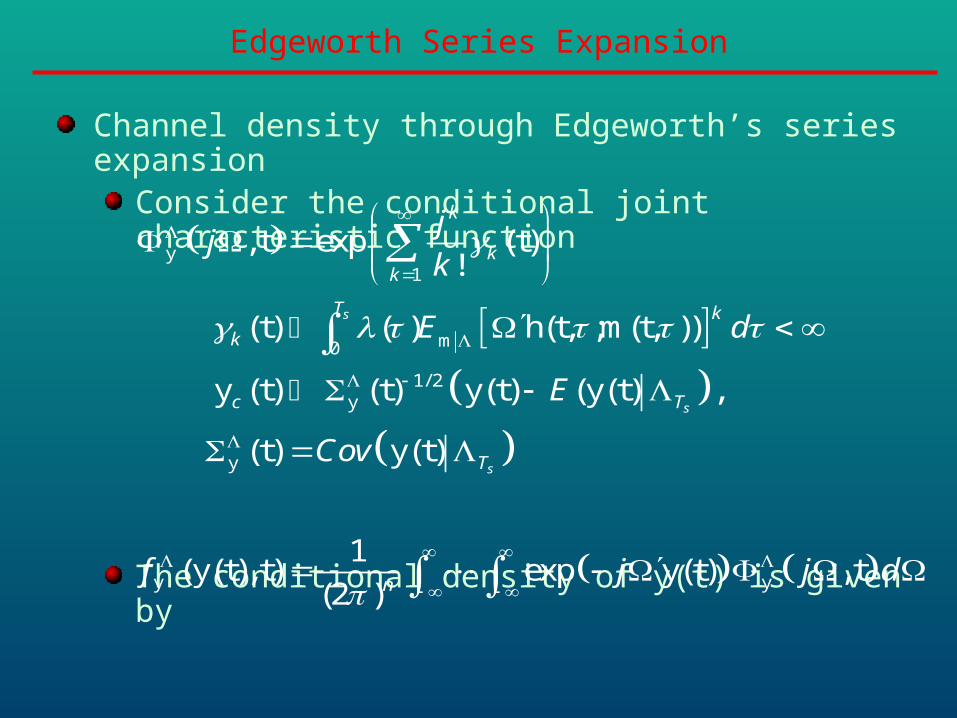
Channel density through Edgeworth’s series expansionConsider the conditional joint characteristic function

The conditional density of y(t) is given by

Edgeworth Series Expansion

y1

m0

1/ 2y

y

y y

, t exp (t)!

(t) ( ) h(t, ;m(t, ))

y (t) (t) y(t) (y(t) ,

(t) y(t)

1(y(t), t) exp y(t) , t

(2 )

s

s

s

k

kk

T k

k

c T

T

n

jj

k

E d

E

Cov

f j j d

Channel density through Edgeworth’s series expansion

First term: Multidimensional GaussianRemaining terms: deviation from multidimensional Gaussian density

Edgeworth Series Expansion

1y (t )y (t )

21/ 2/ 2

y

1/ 2y y

3 4 62

3 4 32

y

1(y(t), t)

(2 ) (t)

1 1exp (t) y (t)- (t)

(2 ) 2

(t) (t) (t)3! 4! 2 3!

First term (y(t) ); (t)

c c

s

yn

cn

T

f e

j

j j jd

N E

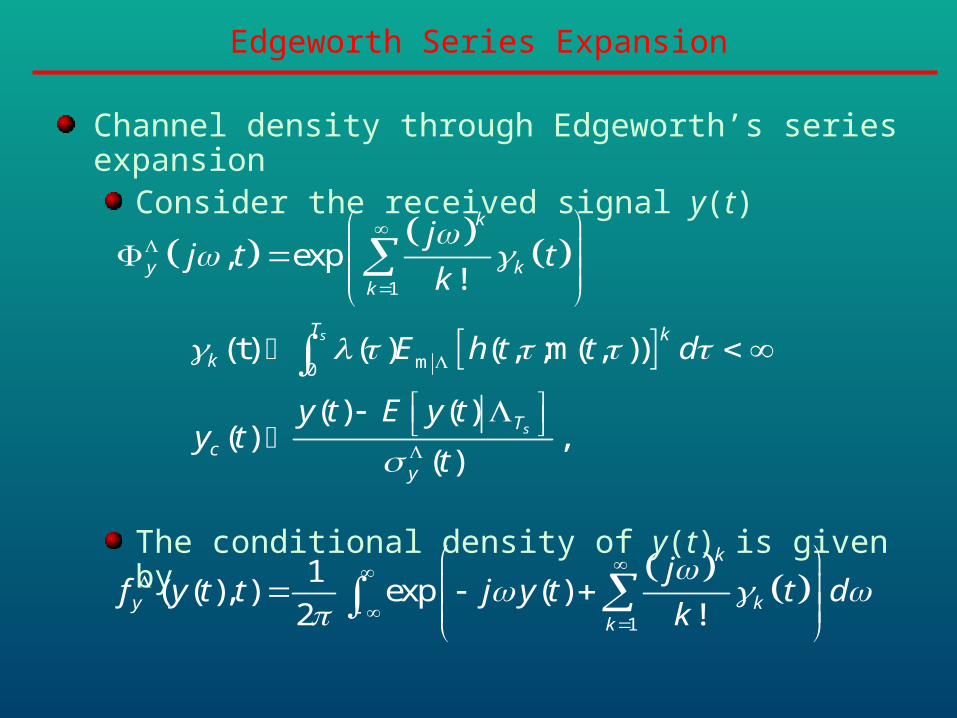
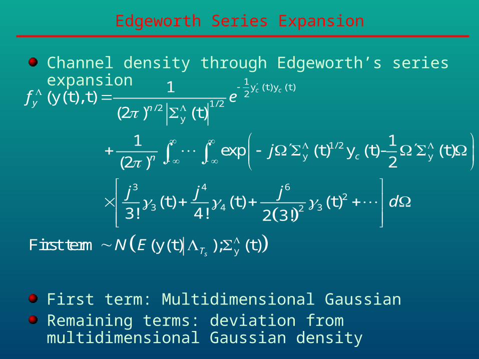
Channel density through Edgeworth’s series expansionConsider the received signal y(t)

The conditional density of y(t) is given by

Edgeworth Series Expansion

1

m0

1

, exp!

(t) ( ) ( , ;m( , ))

( ) ( )( ) ,

( )

1( ( ), ) exp ( )

2 !

s

s

k

y kk

T k

k

T

cy

k

y kk

jj t t

k

E h t t d

y t E y ty t

t

jf y t t j y t t d

k

Conditional density of y(t)

Remaining terms: deviation from Gaussian density

Edgeworth Series Expansion

2

1 (0)y

3 4 (3)3

4 5 (4)4

26 7 (6)3

2

( ) / 2

( ( ), ) ( ) ( )

( )( 1) ( ) ( )

3!

( )( 1) ( ) ( )

4!

( )1( 1) ( ) ( )

2! 3!

1where ( )

2

First term ( ( ) );s

y c

y c

y c

y c

nn x

c n

T y

f y t t t y t

tt y t

tt y t

tt y t

dy t e

dx

N E y t

2( ) : Gaussiant

Received Signal Density: Example

( )

1

Band pass representation of received signal

( ) ( ; ) cos ( ; ) ( )

( ; ) ( ) ( ) ( )

( ) 2 cos ( ) : Doppler frequency

( ; ): signal attenuation coeffici

sN T

i i c i i l ii

i i i c di i di

di m i

i

y t r t t t s t

t t t t t

t f t

r t

0

ent, i.e. Rayleigh, Ricean

, ( ) : time delays and number of paths

( ) : arbitrary low-pass transmitted signal

(t) ( ) ( ; ) cos ( ; ) ( )s

i

l

T kk kk c l

N t

s t

E r t E t t s t d

Conditional density of y(t)

Received Signal Density: Example

1 (0)

4 5 (4)4

6 7 (6)6

29 (84

0

)2

( ( ), ) ( ) ( )

( )( 1) ( ) ( )

4!

( )( 1) ( ) ( )

6!

( )1( ) ( )

2! 4!

1 1( ) ,

1 2 1(t) (

0,2 , ( ) , 0

) (2 !

, 22 2

s

y y c

y

T

k n

c

y c

y c

f y t t t y t

tt y t

tt y t

tt y t

p p

nE r t

n

; ) ( )k k

ls t d

Conditional density of y(t): Rayleigh channel, Constant rate, Transmitted signal: narrow band

First term: centered Gaussian density

Remaining terms decrease as (Ts) increasesVariance of received signal depends on characteristics of environment () and transmitted signal (Ts)Oscillatory behaviour due to basis functions (n)(x)

Received Signal Density: Example

2 2 22

(0) (4)1/ 2

(6) (8)22 2

(10)3

( ) ( ) ( )

1 3( ( ), ) ( ) ( )

( ) 4!

1 15 1 9( ) ( )

6! ( ) 2! 2! ( )

2 45(

( ) ; ( ) ;

)4!6!( )

y s

y c cs s

c cs

c

l

s

s

t t K T

f y t t y t y tK T T

y t y tT T

t s t K

y tT

Channel density through Edgeworth’s series expansion

Constant-rate, quasi-static channel, narrow-band transmitted signal

Received Signal Density: Example; Simulation

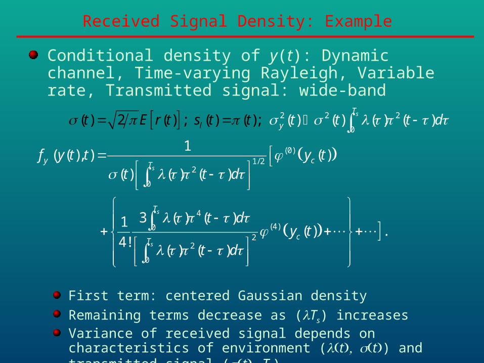
Conditional density of y(t): Dynamic channel, Time-varying Rayleigh, Variable rate, Transmitted signal: wide-band

First term: centered Gaussian density

Remaining terms decrease as (Ts) increasesVariance of received signal depends on characteristics of environment (tt) and transmitted signal (tTs)

Received Signal Density: Example

2 2 2

0

(0)1/ 2

2

0

4

(4)02

2

0

( ) ( ) ( ) ( )

1( ( ), ) ( )

( ) ( ) ( )

3 ( ) ( )1( ) .

4!( )

( ) 2 ( ) ; ( ) ( );

(

)

s

s

s

s

T

l y

y cT

T

cT

t t t d

f y

t E r t s

t t y tt t d

t dy t

t d

t t

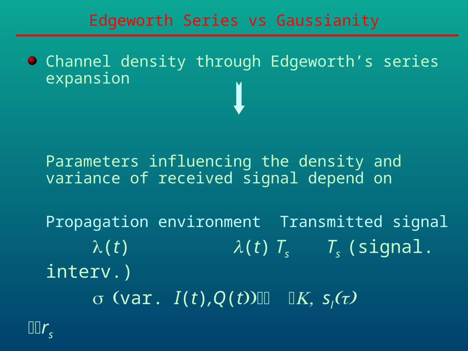
Channel density through Edgeworth’s series expansion

Parameters influencing the density and variance of received signal depend on

Propagation environment Transmitted signal

(t) (t) Ts Ts (signal. interv.)

var. I(t),Q(tslrs

Edgeworth Series vs Gaussianity

Received signal densityis not Gaussiancan be computed through Edgeworth’s series expansion

Methodology brings forward the parameters influencing the density and variance of received signal

depend on propagation environment depend on transmitted signal

Characterization of received signal density is important in the design of transmitters and receivers

Conclusions