arX

iv:1

710.

0779

8v1

[ph

ysic

s.ch

em-p

h] 2

1 O

ct 2

017

An efficient multi-scale Green’s Functions Reaction

Dynamics scheme

Luigi Sbailo1 and Frank Noe 1

1Department of Mathematics and Computer Science, Freie UniversitatBerlin, Arnimallee 6, 14195 Berlin, Germany

October 24, 2017

Abstract

Molecular Dynamics - Green’s Functions Reaction Dynamics (MD-GFRD) isa multiscale simulation method for particle dynamics or particle-based reaction-diffusion dynamics that is suited for systems involving low particle densities. Par-ticles in a low-density region are just diffusing and not interacting. In this caseone can avoid the costly integration of microscopic equations of motion, such asmolecular dynamics (MD), and instead turn to an event-based scheme in which thetimes to the next particle interaction and the new particle positions at that timecan be sampled. At high (local) concentrations, however, e.g. when particles areinteracting in a nontrivial way, particle positions must still be updated with smalltime steps of the microscopic dynamical equations. The efficiency of a multi-scalesimulation that uses these two schemes largely depends on the coupling betweenthem and the decisions when to switch between the two scales. Here we presentan efficient scheme for multi-scale MD-GFRD simulations. It has been shown thatMD-GFRD schemes are more efficient than brute-force molecular dynamics simu-lations up to a molar concentration of 102µM . In this paper, we show that thechoice of the propagation domains has a relevant impact on the computational per-formance. Domains are constructed using a local optimization of their sizes anda minimal domain size is proposed. The algorithm is shown to be more efficientthan brute-force Brownian dynamics simulations up to a molar concentration of103µM and is up to an order of magnitude more efficient compared with previousMD-GFRD schemes.

1 Introduction

Particle-based reaction-diffusion simulations have been widely used to simulate signal-ing cascades in biological systems [1–5]. In contrast to other approaches to simulatemolecular kinetics simulations, such concentration-based approaches or Gillespie’s dy-namics [6,7], the trajectory of all interacting particles is resolved, providing a reaction ki-netics model with high spatio-temporal detail. Particles diffuse according to the Langevin

1

equation, and whenever they are close to each other reactions can happen. In a brute-force approach, all particles are simultaneously propagated over a fixed integration step– at sufficiently long timescales typically using a time-discretization of the overdampedLangevin, or Brownian dynamics (BD) equation [8]. Unfortunately, a short integrationstep is generally required to avoid systematically missing particle interactions [9]. Ininteracting-particle reaction-diffusion (iPRD) simulations, particles are interacting withnonlinear potentials at close distances, which requires even shorter time steps in the BDintegrator [10, 11]. Especially in biological applications, where many proteins may in-teract in a crowded environment to give rise to some supramolecular machinery, suchdetailed simulations may be required [12–14]. However, this approach becomes com-putationally expensive with large particle numbers, and also when fast-diffusing speciesare involved that require small simulation time steps, making it challenging to reachbiologically relevant time scales [1, 15]. Hence, designing efficient multi-scale reaction-diffusion algorithms that can reach the biologically relevant resolution where required,but avoid unnecessary computation time wherever possible, is of high relevance for thebio-simulation community.

One possible strategy adopted to improve computational performances in particle-based simulations is implementing an event-based algorithm as in the first-passage ki-netic Monte Carlo (FPKMC) algorithm [16–18] and Green’s functions reaction dynamics(GFRD/eGFRD) [2, 4, 19]. The central idea is to directly sample the next time point atwhich particles will interact, e.g. to perform a reaction, rather than simulating the trivialdiffusion of free particles via BD. GFRD is synchronous and approximate: in every itera-tion of the algorithm, an integration step length is chosen such that at most two particlescan interact; particles are propagated for that time and eventually react [4,19]. Depend-ing on the system configuration, a new integration step is selected. This algorithm maysuffer from inaccuracies because a finite propagation time always results in a finite choiceof interactions between more than two particles simultaneously, which is not covered bythe algorithm.

In the subsequent asynchronous versions, firstly proposed in FPKMC [16–18] and thenin eGFRD [2], the volume of the system is decomposed into non-overlapping protectivedomains containing one or at most two particles. In each of these domains a next eventis sampled. Events comprise domain escapes, unimolecular reactions, or bimolecularreactions in domains containing two particles. In this asynchronous scheme, a list of allscheduled events is initially compiled, then at every step the system jumps to the nextevent and the list gets updated with a new event. However, some unscheduled eventscan occur and the list must then be updated on the fly. For example, when a particleis about to enter a protective domain, this domain must be burst, i.e. destroyed, theparticle positions must be sampled prematurely, and new protective domains must bedrawn.

A recent extension of this algorithm is the multi-scale combination of explicit time-step integration (for the sake of generality called molecular dynamics (MD), althoughin many practical cases BD will be used) and FPKMC/eGFRD, in short MD-GFRD[20, 21]. In MD-GFRD, interacting particles, i.e. particles that are close in space, aresimulated via short time steps, whereas isolated particles are propagated via an event-based FPKMC/eGFRD scheme on longer time scales, protective domains thus can containonly one particle. Using direct time-integration at short distances allows to incorporate a

2

variety of effects that are relevant to describe molecular detail. For example, these localdynamics could involve momenta [20], anisotropic diffusion [21,22], nonlinear interactionpotentials or complex reactions [10], and would be a natural place to include the dynamicssimulated by kinetic models obtained from all-atom MD, e.g. Markov State Models(MSMs) [23–27] or multi-ensemble Markov models (MEMMs) [28, 29].

MD-GFRD has been shown to be several order of magnitudes faster than brute-forceintegration of Brownian dynamics [20, 21]. The efficiency improvement is particularlyevident in dilute systems, where particles spend most of their time freely diffusing inthe system before encountering each other, which renders an event-based algorithm, thatdirectly samples encountering times, dramatically faster. However, this efficiency is lost athigh densities, while the efficiency of direct time-step integration is only mildly dependenton the particle density (e.g. through the number of neighbor interactions that need to beevaluated in each time step). Indeed, constructing a domain and sampling an event init is computationally more demanding than performing few brute-force Brownian motionsteps. Therefore, one typically avoids the construction of very small domains that wouldburst rapidly, and instead uses direct time-step integration when the size of a newlyconstructed domain is below the minimal domain size [20, 21, 30]. Still, as the systembecomes more dense, the efficiency of this scheme decreases, as the fraction of particlesthat are described by direct time-step integration increases, and domains, which arerequired to be non-overlapping, tend to be smaller and thus more prone to a prematureburst. In this context, determining the optimal size of the minimal domain and avoidingunnecessary, premature bursts can be critical to ensure computational performance.

In this paper, we present a domain making scheme and several numerical improve-ments that make multi-scale FPKMC/eGFRD algorithms such as MD-GFRD more ef-ficient. The main developments are the determination of the optimal domain size uponconstruction and of the minimal domain size for the construction of small domains.

2 Molecular Dynamics - Green’s Function Reaction

Dynamics

We briefly introduce into MD-GFRD in order to summarize the concepts relevant for thepresent paper. In MD-GFRD, the system is decoupled into non-overlapping sphericaldomains, or shells, that contain at most one particle. MD-GFRD is an event-basedalgorithm, whose events are particle escapes from their protective domain. The eventtimes are obtained by sampling from a Green’s function as explained below.

Brownian motion can be described probabilistically by the Einstein diffusion equation,

∂p(~r, t)

∂t= D∆p(~r, t), (1)

where p(~r, t) is the probability distribution of a Brownian particle with diffusion coefficientD, ~r = (r, θ, φ)⊤ is the position of the particle and ∆ is the Laplace operator in sphericalcoordinates. Isolated particles are treated using Green’s function dynamics. To facilitatethat, one creates spherical “protective” domains of radius b around them, in order tomark the volume within which they can diffuse without interacting with other particles.The domain size b is chosen such that it contains only one particle and the whole sphere’s

3

volume is not subject to any external potentials, i.e. the interaction of other particles,membranes, etc. Given the spherical symmetry of this problem, the evolution of theprobability distribution can be described by the radial function p(r, t), which representsthe probability to be in any point on the surface of a sphere of radius r. The radialprobability to be at a radius r < b, without having previously hit the domain border b, iscomputed by imposing absorbing boundary conditions on the domain borders, p(b, t) = 0[31]. By imposing this boundary condition and the initial condition p(r0, t0) = δ(r0) onEq. (1), we obtain:

p(r, t|r0 = 0, t0) =1

S(t)

∞∑

m=1

exp

{−m2π

2D

b2(t− t0)

}2πr

b2m sin

(mπr

b

), r < b. (2)

S(t) is the survival probability

S(t|r0 = 0, t0) = −2

∞∑

n=1

(−1)n exp

{− n2π

2D

b2(t− t0)

}, (3)

which represents the probability that the particle is inside the domain at t, without havingpreviously hit the borders. The first exit time probability q(t) is defined via the survivalprobability S(t)

q(τ |r0 = 0, t0) = −dS(τ)

dτ= −2

∞∑

n=1

(−1)n exp

{− n2π

2D

b2(τ − t0)

}n2π2

b2D, (4)

and it gives the probability that the particle escapes its domain for the first time at τ .In this derivation, we have assumed that no other particles enter the domain, and the

particle inside the domain is not subject to any external potentials or forces (e.g. exertedby particles near the domain). However, in a multi-particle simulation this assumptionis not always valid. Let us assume that at t0 we have constructed a protective domainaround an isolated particle, and this particle has sampled a first exit time t0 + τ fromits domain. In this situation, it is possible that an external particle, whose motion isbrute-force integrated, is in proximity to the first domain at a time, t1 < t0 + τ , i.e.before the escape time. The first exit time τ has been sampled assuming that no otherparticle interact with the domain, hence the intrusion of another particle before that timewould make the sampling of the particle’s escape time invalid. Consequently, to ensurethat particles in protective domains are freely diffusing, we define a burst radius for eachpair of particles to be at least the interaction length between the intruding particle andthe particle in the domain. Whenever a particle approaches a protective domain to adistance below the burst radius the domain is burst, i.e. destroyed. In that event, theparticle position is updated inside the domain by sampling eq. (2) at time t = t1. Aftera domain burst, the clock of the two particles is synchronized to t1.

2.1 Algorithm outline

In MD-GFRD, the particle propagation is performed alternatively via direct time-step in-tegrations or Green’s functions samplings. The choice of the propagation method depends

4

5) 6)

3)

4)

1) 2)

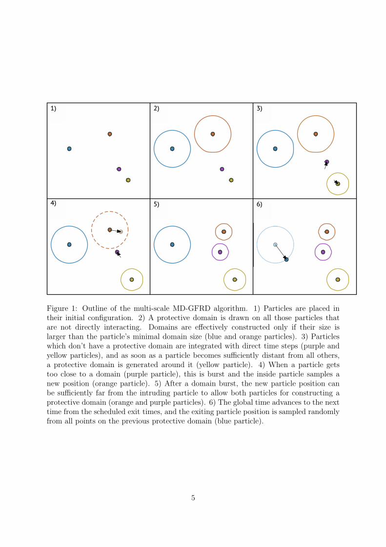
Figure 1: Outline of the multi-scale MD-GFRD algorithm. 1) Particles are placed intheir initial configuration. 2) A protective domain is drawn on all those particles thatare not directly interacting. Domains are effectively constructed only if their size islarger than the particle’s minimal domain size (blue and orange particles). 3) Particleswhich don’t have a protective domain are integrated with direct time steps (purple andyellow particles), and as soon as a particle becomes sufficiently distant from all others,a protective domain is generated around it (yellow particle). 4) When a particle getstoo close to a domain (purple particle), this is burst and the inside particle samples anew position (orange particle). 5) After a domain burst, the new particle position canbe sufficiently far from the intruding particle to allow both particles for constructing aprotective domain (orange and purple particles). 6) The global time advances to the nexttime from the scheduled exit times, and the exiting particle position is sampled randomlyfrom all points on the previous protective domain (blue particle).

5

on the system configuration and, in particular, whether the particle is freely diffusing orinteracting with other particles. At each iteration of the algorithm, one particle is selectedfrom a time-ordered event-list. If this particle is not interacting with other particles, theconstruction of a protective domain is attempted. The construction is then accepted onlyif the domain radius is larger than the minimal domain size, whenever the constructionis rejected the particle motion is instead brute-force integrated.

In this scheme, particle interactions are always evaluated on discrete times {tn}, wheretn = n dt, n is an integer, and dt is the MD integration step. Therefore, a GFRD particlethat leaves a protective domain and thus becomes an MD particle is mapped to thenext discrete time via a small Brownian motion step. MD particles that are evaluatedat the same time point t can be updated simultaneously and collectively as in usualMD implementations. In the following pseudocode, however, it is simpler to explain thealgorithm as if all particles are treated by an asynchronous event list.

Each particle possesses a current and a scheduled position and time. Each particleis also associated with an event, that takes the particle from its current position andtime to its scheduled position and time, if it is successfully executed. Events include MDintegration step and scheduled exits from a protective domain, but they may be modifieddue to events such as domain bursting. In the beginning of the simulation, the domainmaking algorithm creates a protective domain for each particle that is not involved ina direct interaction. Domains larger than the minimal domain size ρ are constructed,and first exit times are sampled via Eq. (4). These exit events are then stored in a listordered by increasing scheduled-time. All particles that could not construct a protectivedomain are placed on top of the event-list, forces between them are computed and theirscheduled positions are computed and stored. Based on this initial list, the followingasynchronous algorithm propagates the system state in time:

1. Pick the first particle i in the event-list:

(a) If the particle was in a protective domain: place it on a position sampleduniformly at random on the domain boundary. Then, propagate it to the nextdiscrete time ti via a free Brownian motion sampling.

(b) Else: update the particle position and time to the stored scheduled positionand time.

2. Compute the distances {rij}Nj=1 from the N neighboring particles. The distances arebetween the centers of mass and are computed between synchronous positions whenparticles are not located in a protective domain; otherwise, the distance betweenthe center of mass of the particle i and the center of the protective domain of theparticle j is computed.

3. For all j = 1, ..., N : if the particle j is in a protective domain and the i− j distanceis below the burst radius (rij − rj < Ri

burst, where rj is the domain size of theparticle j):

(a) Burst the j-domain.

(b) Synchronize the scheduled time of particle j to ti and update the scheduledposition of particle j by sampling from Eq. (2).

6

(c) Place particle j on top of the event-list.

(d) Update the rij distance.

4. Use the distances {rij}Nj=1 , where rij = rij −Rijint and Rij

int is the interaction length,in a domain making algorithm to create a domain with radius ri:

(a) If the proposed radius is larger than the minimum domain size, ri > ρi: acceptthe domain, sample the first exit time τi from Eq. (4), and increase the particleevent time by τi.

(b) Else: Update the scheduled position and scheduled time via direct time-steppropagation (this step might involve also interactions and reactions).

5. Place the particle i in the event-list according to increasing event time.

Note that if particles i and j construct domains that are in contact and if followingstep 1a these particles have identical scheduled discrete exit times, it is possible that theparticle i, upon escape, bursts the j-domain at a later time than the scheduled exit timeof particle j. This apparent inconsistency is due to the fact that in this serial algorithmparticle j has not executed the step 1a yet. Clearly, in this occasion the position ofparticle j is updated by executing the step 1a rather than sampling from Eq. (2).

In Fig. 1, a graphical representation of a possible outcome of this algorithm is shown;there is not a match between the points in the algorithm and the points in the figure.

3 Domain making scheme and minimal domain size

The basic idea of domain making schemes is that larger domains correlate with moreefficient computation, as the particle doesn’t participate in direct time-step integrationduring the correspondingly longer exit times (see Eq. (4)). However, choosing domainsizes in a greedy manner does not necessarily lead to optimal performance. For instance,when a large domain is next to a much smaller one, or to a domain close to its escapetime, the latter domain is likely to experience a particle exit very soon, which mightin turn burst the large domain, thereby annihilating the advantage of the long exit timefrom that domain. Domain bursting is not convenient, since it involves sampling a secondGreen’s function. Moreover, it represents an unscheduled event that is difficult to treatefficiently in a parallel implementation.

The minimal domain size determines whether the domain construction is acceptedor not. Instead of sampling the first exit time from a small domain, it might be moreconvenient to simulate the same particle propagation via direct time-step integrations.Indeed, solving a first exit time problem has generally a higher computational cost thansimulating a number of direct time-step integrations. Thus, in MD-GFRD algorithms,the dimension of the smallest domain whose construction is allowed must be determined:whenever the construction of a domain of smaller size is attempted, this trial is rejectedand the particle is instead brute-force integrated.

7

Rint

(a)

GF

r

Rint

(b)

BM

r

i

i

j

j

r i

r i

rj

Figure 2: MD-GFRD domain making scheme suggested in [20, 21]. The domain sizechoice is made according to the status of the neighboring particle: a) the prime neighboris a GF particle, then the shell takes all available space; b) the prime neighbor is a BMparticle, then only half of the available space is used.

3.1 MD-GFRD

The MD-GFRD domain making schemes employ the largest shell principle to draw protec-tive domains. We distinguish between Green’s function (GF) particles which are locatedin a protective domain and Brownian motion (BM) particles that are undergoing a directtime-step integration. The domain making routine firstly computes the center-center dis-tance rij between the particle i of interest from all neighboring particles j, subtractingthe interaction length Rij

int of the particle pair. The resulting distance rij = rij − Rijint is

then divided by 2 if the particle j is a BM particle. If the particle j is a GF particle, thedistance is reduced by the j-domain size rj (Fig. 2). In the case of a BM particle onlyhalf of the total distance is used to let the other particle construct a domain of equal sizein the subsequent step. This routine is iterated over all neighboring particles and thelowest value obtained is finally selected. This domain creation makes domains as largeas possible while avoiding direct particle interaction.

In previous studies, the minimal domain size in MD-GFRD algorithms has been setproportional to the particle radius [20, 21, 30], where the sum of the particles radiigives the particles pairwise interaction. In particular, the minimal domain size has beensuggested to be always larger or equal than the particle radius [30]. In the implementationof Ref. [21], the minimal domain size ρ is chosen to be equal to the particle radius. In theimplementation of Ref. [20], ρ can have different values depending on whether the particleis undergoing a direct time-step integration (ρGFRD) or has just escaped a protectivedomain (ρBD). The minimal domain value assumes a larger value when the particle isunder direct time-step integration (ρGFRD > ρBD). This technique has been used to

8

(1)

r i,1rj

r

Rint

rnext

i j

j'

(2)

ri,2

i j

r j'

r i,1

Figure 3: New domain making scheme for the case of an isolated pair of particles. Attime ti, particle i is attempting the construction of the i-domain close to particle j thatis already enclosed in a domain. The escape time tj′ > ti and particle j’s escape positionwere sampled when the domain was constructed. 1) Particle i constructs a domain whosesize ri,1 is such that its average first exit time is the same as the average first exit timeof particle j from the j′-domain that might be constructed after the exit from its currentj–domain. 2) The domain size in the previous step obtained is further reduced to finallyobtain ri,2.

prevent particles from rapidly switching between the GF and BM mode. Indeed, whenthe particle motion is subject to direct time-step integration, it is likely to be located ina crowded region of the system, where a domain is more likely to be burst. Diminishingthe number of domains constructed in this regions correlates with a lowering of the totalnumber of bursts. This scheme has been used to simulate particles interacting via aLennard-Jones potential, and the minimal domain values ρGFRD = 5σ and ρBD = 3σwere used, where σ is the Van-der-Waals radius.

Finally, the bursting radius should be chosen equal or larger than the interactionlength of the two particles. However, it cannot be larger than the minimal domain size ofany other particle to prevent the algorithm from entering in an infinite mutual burstingloop, where a pair of isolated particles alternatively construct a domain which is burst bythe other particle in the subsequent step. In MD-GFRD, the bursting radius is set equalto the interaction length plus the minimal domain size of the particle, because whenever aparticle is close to another domain, that domain must be burst in order to allow creatingtwo new domains of significant size.

9

3.2 New domain-making scheme

The aim of the new scheme is to improve the algorithm’s computational performanceand to decrease the number of domain bursting events. In order to keep the number ofbursting events small, domains are sized such that they have the same average first exittime as the domains that will be constructed in their proximity. The key idea is thatwhen domains are constructed, not only the first exit time of the particle is sampled, butalso its exit position. This information is used by neighboring particles to propose anoptimized domain size such that it has the same average first exit time as the domainsthat will be later constructed on the memorized exit positions (Fig. 3 1). In Ref. [18]the importance of constructing optimized domains has already been discussed, and it issuggested that domains should be constructed to delay in time as far as possible the firstevent in the queue, which corresponds to constructing domains with equal mean first exittimes. However, this was achieved only when all domains are constructed simultaneously,which optimizes only over the first event in queue. By pre-sampling the exit position ofparticles, it is instead possible to construct balanced domains over a long series of events.Although developed for MD-GFRD, the idea of pre-sampling the exit position can alsobe applied to FPKMC/eGFRD schemes.

In order to further reduce the number of bursting events, the domain size is thenshrunk. Although the domains are not chosen to be of maximum size, this approachsignificantly reduces the overall number of bursts compared to the scheme described inSec. 3.1. The choice for the size reduction in the second step (Fig. 3 2) is performed toobtain a balance between a low number of bursts and long domain exit times. Clearly,the specific setting of these parameters depends on implementation details such as serialor parallel execution etc, and can be adapted to the local setting. This algorithm isillustrated in the simplest case of an isolated pair of particles in Fig. 3. In the newscheme, the bursting radius is also chosen to be equal to the interaction length plus theminimal domain size.

In practice, if the domain is created close to a GF particle (Fig. 3 1) the first domainri,1 is obtained by solving a system of two equations:

r2j′

6Dj

+∆t =r2i,16Di

, (5)

rnext = ri,1 + rj′, (6)

where rnext = rnext−Rint is the available space, rnext is the distance between the center ofparticle i and the exit position of particle j, ∆t = tj′ − ti is the time difference betweenthe scheduled exit time of particle j and the current time, i.e. the time in which particlei is attempting to construct a domain. The first equation imposes that the average exittime from the i-domain is the same as from the j′-domain, where the expected exit time〈τ〉 of a Brownian particle with diffusion coefficient D from a sphere of radius b is:

〈τ〉 = b2

6D. (7)

The second equation enforces the domains to be adjacent by taking all available space,according to the largest shell principle. In contrast to MD-GFRD, the largest domain

10

principle is applied between the i-domain and the j′-domain that is possibly constructedsubsequently.

If the average first exit time of particle i from the available space ri,1 = rnext is lessthan ∆t, the time interval to the scheduled exit time of particle j, the solution of thesystem in Eq. (5) has no real values, which means that the i-domain and the j′-domaincannot have the same average first exit time. As the j-particle is not expected to burstthe i-domain in this case, we use all available space for the i-domain, i.e. ri,1 = rnext.Consistently, inserting ∆t = r2next/6Di in Eq. (5) results in the solution ri,1 = rnext.

The system in Eq. (5) is then solved only when ∆t < r2next/6Di. The optimal domainsize is then given by:

ri,1 =

rnext, ∆t ≥ r2next

6Di.

rnext1−

√1−(1−

Dj

Di)(1+

6∆tDj

r2next

)

1−Dj

Di

, otherwise.(8)

The square root argument in Eq. (8) is always positive if ∆t < r2next/6Di, therefore thesolution is always real-valued. The boundary condition 0 < ri,1 < rnext has been applied,as explained in Appendix A.

If the two particles have identical diffusion coefficients D, the solution simplifies to:

ri,1 =rnext2

+3D∆t

rnext. (9)

The value ri,1 obtained is a function of the distance rnext. Hence, ri,1 does not take thevolume of the existing j-domain into account and thus does not ensure to avoid overlap ofthe i and j domains. To avoid such an overlap, the i-domain must be accordingly resizedto the largest possible value: ri,1 = r − rj , where r = r − Rint and r is the center-centerdistance between particles i and j.

A similar approach is used if particle j is a BM particle. In this case, the i-domain iscreated so as to leave enough space for particle j to construct a domain whose first exittime is equal to the i-domain:

ri,1 =r

1 +√

Dj

Di

. (10)

Finally, the domain radius is further reduced as :

ri,2 = ri,1 − nred

√2Dj dt, . (11)

where nred is a parameter (Fig. 3 2). The domain reduction is set proportional to theaverage displacement that the particle j performs in one integration step. This reductionis performed to reduce the probability that the particle j bursts the i-domain in caseswhere the sampled escape time of the particle i is larger than the expected value. Notethat if ∆t > r2i,1/6Di the particle j is expected to escape its domain after the particle i,in this case there is no need to reduce the size of the i-domain and thus the step in Eq.(11) is omitted. When this scheme is applied to multi-particle systems, the previouslyoutlined approach is applied to all nearest-neighbor particle pairs, and the lowest valueof ri,2 is chosen.

11

0 2 4 6 8 10

D [µm2

s ]

0.00

0.05

0.10

0.15

0.20

0.25

0.30

ρ[nm

]

Figure 4: Minimal domain radius ρ as a function of D using the time step dt = 0.1ns.The dots represent the radius of the minimal protective domain where Green’s functionssampling and direct time-step integration have equal CPU costs. Simulations to computethe first exit time from the domain with size ρ were conducted for different diffusioncoefficients and domain sizes, using either direct time-step integration or Green’s func-tions sampling. For small domain sizes, the direct time-step integration is always moreefficient. The dashed red line shows ρ = α

√Ddt, as described in Eq. (16), with the

implementation-specific value α = 8.4 that has been found empirically.

3.3 New scheme for minimal domain size

In contrast to previous works, the minimal domain size is proposed here to be propor-tional to the square root of the particle diffusivity, rather than the particle size. Theminimal domain size defines the particle distance below which direct time-step integra-tion is assumed to be more efficient than sampling Green’s functions. We assume thatthe CPU time required to sample the probability density of the first exit time is approx-imately independent of domain size and diffusion coefficient. In contrast, the CPU timespent to simulate first exit times via brute-force integrations depends on the domain size,on the particle diffusion coefficient and on the time-step length.

Given the average first exit time 〈τ〉 of a particle with diffusion coefficient D from asphere of radius b, Eq. (7), the average number of steps 〈n〉 to simulate the first exit timeis:

〈n〉 = b2

6Ddt, (12)

where dt is the time step. The average CPU time, 〈TBF (b)〉, spent to compute escapetimes via brute-force integrations is proportional to the number of integration steps, andthus:

〈TBF (b)〉 ∝b2

Ddt. (13)

It is assumed that the average CPU time, 〈TGF (b)〉, spent to sample a Green’s functionis approximately constant.

〈TGF (b)〉 = Const. (14)

12

Let ρ be the domain size at which the CPU times are equal, 〈TBF (ρ)〉 = 〈TGF (ρ)〉, then:

ρ2 ∝ Ddt. (15)

Hence, the minimal domain radius ρ(D, dt) is defined as the threshold that determineswhether the domain construction is accepted or not.

ρ(D, dt) = α√Ddt. (16)

Simulations indicate that this function correctly describes the point where a direct time-step integration becomes more efficient than a Green’s function root finding (Fig. 4).The parameter α is a value that depends on the implementation and machine, and isdetermined in the beginning of a simulation (see Appendix B).

4 Results

We compare the performance of the multi-scale MD-GFRD scheme implemented in Refs.[20] and [21], the new scheme, and a direct time-step integration scheme using Browniandynamics. Two versions of the new scheme are simulated, one with nred = 5 in Eq.(11) (new scheme 1), and one which does not use domain size reduction (nred = 0, newscheme 2), thus tending to size domains more greedily. In addition, we also test a hybridscheme, which implements the minimal domain size as described in Sec. 3.3 but employsthe same domain making scheme as proposed in Refs. [20] and [21]. For simplicity wesimulate particles in a periodic box and interacting with a harmonic repulsion:

V (r) =1

2k (Rint − r)2, r < Rint, (17)

where r is the inter-particle distance between the centers of mass, k = 100 is the springconstant, and the interaction length Rint is equal to the sum of particle radii. Reac-tions, more complex particle-particle potentials, or other near-space interactions can bestraightforwardly integrated in the direct time-step integration regime that is used tosimulate interacting particles.

Two simulations have been performed using different diffusion coefficients and particleradii:

1. 10 spherical particles with radiusR = 2.5nm and diffusion coefficientD = 10µm2/s.

2. 5 faster and smaller particles with radius R1 = 1.5nm and diffusion coefficientD1 = 10µm2/s and 5 slower and larger particles with radius R2 = 3.5nm anddiffusion coefficient D2 = 1µm2/s.

4.1 Efficiency comparisons of different MD-GFRD schemes anddirect Brownian dynamics

To obtain clean benchmarks, most calculations are run with ten particles and directevaluation of all pairwise particle distances, while the particle density is adjusted by

13

choosing the box size. For a more complex test, Sec. 4.3 simulates larger particle numberswith a neighbor list implementation.

The efficiency of MD-GFRD strongly depends on the particle concentration, since incase of dilute systems particles are allowed for constructing large domains and performinglarge time steps. Hence, MD-GFRD algorithms are dramatically faster than BD schemesat low concentrations. As the particle concentration is increased, MD-GFRD becomesless efficient, while the BD efficiency remains constant. Consequently, there is a concen-tration threshold where BD starts being more efficient than MD-GFRD. In Fig. 5, theperformance is compared between the new schemes, the hybrid scheme, the previous MD-GFRD schemes and direct BD simulation. It is evident that all MD-GFRD schemes areseveral order of magnitude faster than BD at low densities. Moreover, the new schemesare faster than the previous MD-GFRD schemes at all densities, but performances aresimilar at low densities. In particular, for both diffusion coefficients, the new schemesand the hybrid scheme are preferable over BD for concentrations up to 103 µM, whereasprevious MD-GFRD schemes were preferable over BD only up to molar concentrationsof 102 µM. The schemes which implement the new minimal domain size all show similarperformance, and among them the new scheme 2 is the fastest. We note that these num-bers may be different in different implementations (codes and machines), and comparisonis therefore only meaningful within the same implementation.

The total number of direct integration time-steps performed in each multi-scale MD-GFRD simulation increases with increasing particle concentration (Fig. 6). This growthis remarkably similar to the growth in the CPU time, indicating that the reason of theimproved performance of MD-GFRD schemes is essentially due to a reduction of thedirect time-integration steps that represent the computational bottleneck. In the newschemes and in the hybrid scheme, the minimal domain size is smaller than in previousMD-GFRD schemes, which enables more protective domains to be constructed, which inturn reduces the fraction of time spent in direct time-step integrations. Although havingequal minimal domain size, the new scheme 2 shows a slightly lower number of directintegration time-steps with respect to the hybrid scheme. This is essentially the resultof the construction of more balanced domains which allow for an optimization of theavailable space. On the other hand, the new scheme 1 spends a larger fraction of timeunder direct time-step integration, because after the reduction step more domains arenot sufficiently large for construction.

14

10−3 10−2 10−1 100 101 102 103

Molar concentration [µM]

10−3

10−2

10−1

100

101

102

CPU

time

[s]

D =10µm2

s

(a)

BD

MD-GFRD 1

MD-GFRD 2

Hybrid scheme

New Scheme 1

New scheme 2

10−3 10−2 10−1 100 101 102 103

Molar concentration [µM]

(b)

D1 =10µm2

s

D2 =1µm2

s

Figure 5: CPU time required to simulate 1ms of real time, using a brute-force integrationstep of dt = 0.1ns. The number of particles is kept fixed to N = 10, while the systemvolume is adapted to the selected molar concentration. Simulations are performed in acubic-shaped box with periodic boundary conditions. Particles are spherical-shaped withradius R = 2.5nm and diffusion coefficient D = 10µm2/s in (a) and radii R1 = 1.5nmand R2 = 3.5nm and diffusion coefficients D1 = 10µm2/s and D2 = 1µm2/s in (b).A binary interaction length is defined as the sum of particles radii, when particles arein within this distance repulse according to a harmonic potential as in Eq. (17), wherek = 100. The minimal domain of the new schemes and of the hybrid scheme uses thepre-factor α = 9 as defined in Eq. (16), see Appendix B. In new scheme 1, nred = 5; innew scheme 2, nred = 0, see Eq. (11). In MD-GFRD 1, the minimal domain size is equalto the particle radius [21]. In MF-GFRD 2, the minimal domain sizes ρGFRD = 2.5Rand ρBD = 1.5R [20] were used, where the pre-factors 1.5 and 2.5 have been chosen toadapt to a different simulation the pre-factors used in Ref. [20], while preserving theirsame relative proportions. At low concentrations, MD-GFRD schemes are several orderof magnitude faster than BD. The new schemes and the hybrid scheme are faster thanBD up to concentrations of 103 µM , while MD-GFRD schemes are preferable over BDup to 102 µM.

15

10−3 10−2 10−1 100 101 102 103

Molar concentration [µM]

101

102

103

104

105

106

107

108

Totalnumber

ofbrute−force

steps

D =10µm2

s

(a)

MD-GFRD 1

MD-GFRD 2

Hybrid scheme

New Scheme 1

New scheme 2

10−3 10−2 10−1 100 101 102 103

Molar concentration [µM]

(b)

D1 =10µm2

s

D2 =1µm2

s

Figure 6: Total number of direct time-steps in the multi-scale MD-GFRD simulationsdescribed in Fig. 5. As the particle density increases, interactions between particlesbecome more frequent, and more simulation time is spent in conducting direct time-stepintegration. The behavior of these curves is similar to that in Fig. 5, indicating that thenumber of brute-force Brownian motion steps represent the bottle-neck in the presentsimulations. The largest value in each plot, 108, represents the condition where eachof the 10 particles have performed 107 direct time-steps, which means that no particlepropagation was made using Green’s functions sampling. In the new schemes and in thehybrid scheme, FPKMC/eGFRD steps are still done 90% of the time under the sameconditions.

16

4.2 Minimization of the domain burst frequency

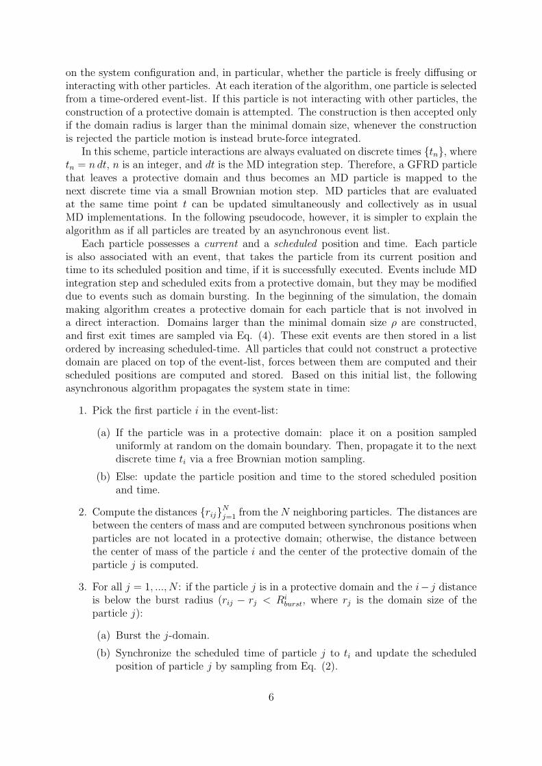
Despite the fact that domain sizes are small on average, Fig. 7 shows that the totalnumber of bursts is the lowest in new scheme 1, i.e. when the domain reduction isincluded. The hybrid scheme involved the highest number of bursts, since the constructionof small domains is allowed, but their sizes are not chosen optimally. The incorporationof particle exit positions into domain construction, and the choice of domain sizes soas to balance the exit times allows to reduce the number of bursts to one third (newscheme 2); if a reduction step is also added (new scheme 1), the number of bursts isfurther reduced by approximately one order of magnitude. This improved efficiency onthe domain construction is evident in Fig. 8, which shows the probability that a protectivedomain is burst prematurely by intrusion of another particle rather than being annihilatedby a regular exit of the particle contained therein. This quantity is computed as the ratioof the total number of domain bursts over the total number of constructed domains.At low concentrations the bursting probability is small, but it increases with increasingparticle density. The new domain-making scheme clearly results in more efficient domainsthat are much less probably to be burst prematurely compared to the previous MD-GFRDscheme, especially at higher concentrations.

The full implementation of the new scheme (version 1) is to be preferred to previousMD-GFRD schemes in both cases: when the serial computational performance is mostrelevant and when the number of total bursts is required to be low. The MD-GFRDimplemented in Ref. [21] is faster than the implementation in Ref. [20], while the latterscheme has a lower number of domain bursts. The new scheme 1 is instead superiorin both computational performance and number of domain bursts. More specifically,the implementation as in new scheme 1 is optimal to drastically lower the number ofbursts while preserving efficiency. The new scheme 2 instead has a slightly higher CPUperformance in our implementation, but does not keep the number of bursts small. Theimprovements result to up an order of magnitude of gain in the CPU performance andan order of magnitude of gain in the total number of bursts.

17

10−3 10−2 10−1 100 101 102

Molar concentration [µM]

10−1

100

101

102

103

104

Totalnumber

ofbursts

D =10µm2

s

(a)

MD-GFRD 1

MD-GFRD 2

Hybrid scheme

New Scheme 1

New scheme 2

10−3 10−2 10−1 100 101 102

Molar concentration [µM]

(b)

D1 =10µm2

s

D2 =1µm2

s

Figure 7: Average total number of protective domain bursts in the multi-scale MD-GFRDsimulations described in Fig. 5. As the molar concentration is increased, domains tendto be smaller and to be constructed more often, which goes along with an increase of thenumber of bursts. The average number of bursts in the new scheme 1 is lower than inthe previous MD-GFRD implementations at any density. Keeping the total number ofbursts low can be important for efficient parallelization, e.g. using Graphical ProcessingUnits (GPUs).

18

10−3 10−2 10−1 100 101 102

Molar concentration [µM]

10−2

10−1

Burstinдprobability

D =10µm2

s

(a)

MD-GFRD 1

MD-GFRD 2

Hybrid scheme

New Scheme 1

New scheme 2

10−3 10−2 10−1 100 101 102

Molar concentration [µM]

(b)

D1 =10µm2

s

D2 =1µm2

s

Figure 8: Domain bursting probability, i.e. ratio of the total number of domains burstover the total number of domains constructed in the MD-GFRD simulations described inFig. 5. The domain construction schemes proposed here are clearly more efficient thanprevious schemes and results in domains that are more likely to survive until the particlescontained therein make successful exits. The bursting probability is always lower than 3%in the new scheme 1, while in the implementations MD-GFRD 1,2 this value is roughlyan order of magnitude larger at the higher concentrations.

19

Table 1: Computational time to simulate 1ms of real time, using a brute-force integrationstep of dt = 0.1ns. Particles are spherical-shaped with radius r = 2.5nm and diffusioncoefficientD = 10µm2/s. A harmonic potential is used to reproduce particles interactionsas in Eq. (17), with k = 100. A linked list cell has been implemented, where each gridbox is a cube with length Lbox = 5nm in BD, and Lbox = 10nm in the new scheme. Inthese simulations the new scheme remains to be more efficient than BD up to a molarconcentration of 103µM .Molar concentration Particles number CPU time, new scheme CPU time, BD

102 µM 103 271 s 14.5 103 s103 µM 104 230 103s 260 103s

4.3 Large particle numbers

The general trends observed in the benchmarks shown in the previous sections arealso expected to hold for systems with many particles. However, in systems with manyparticles n, it is necessary to implement a neighbor list to avoid that each timestep scaleswith n2 as a result of the pairwise distance calculations.

In order to validate that our MD-GFRD scheme can still be efficiently implementedwith many particles, we implemented new scheme 1 with nred = 5 using a neighbor list.Particles are interacting with harmonic repulsion with radius R = 2.5nm, k = 100, andperiodic boundary conditions are applied as described in the previous section. The systemvolume is kept fixed to 17.576 106 nm3, while the number of particles is adapted to achievethe desired molar concentration. All particles have diffusion coefficient D = 10µm2/s.

In order to efficiently implement a neighbor list, we used a discretization of the sim-ulation box in cells of length Lcell = 5nm for the brute-force BD simulations and ofLcell = 10nm for the MD-GFRD simulations. Each particle checks the cell it is locatedin and the 26 neighboring cells for possible neighbors. In such a cell discretization, thesmallest distance at which two particles can loose track of each other is the cell length, andthus the maximum protective domain size must be limited to at most half the cell lengthminus the interaction length, which is the gap to be left between contiguous domains.Here, we limited the maximum domain size to Rmax = 2.5nm.

The simulation results in Tab. 1 show that the new scheme remains to be faster thana brute-force integration up to a molar concentration of 103µM

20

0.00

0.01

0.02

0.03

MSD

[µm

2]

D = 10µm2

s

(a)

0 100 200 300 400 500 600

t [µs]

0.000

0.005

0.010

0.015

MSD

[µm

2]

(b)

D1 = 10µm2

s

D2 = 1µm2

s

BD

MD-GFRD

New scheme

Figure 9: Mean square displacement of particles diffusing, simulated as described in Fig.5 for a molar concentration of 102µM . The MD-GFRD scheme used is from Ref. [21], inthe new scheme a reduction step was performed with nred = 5. The expected value of freediffusing particles (red dashed line) is given by 〈∆r2〉 = 6Dt in (a) and 〈∆r2〉 = 6 D1+D2

2t

in (b). The mean squared displacements are slightly below the mean square displacementsof freely diffusing particles due to crowding effects.

4.4 Mean square displacement

In order to validate the implementation of the MD-GFRD schemes, of the new schemeand of the direct time-step integration scheme used, the mean squared displacement ofthe particles simulated with the different schemes has been recorded and compared. InFig. 9, the mean square displacement shows an excellent agreement between the differentschemes.

21

5 Conclusions

We have described a novel multi-scale MD-GFRD scheme to simulate diffusion and inter-action of Brownian particles. In a multi-scale MD-GFRD scheme, the propagation of freeparticles is performed in an event-based fashion via Green’s functions samplings, whilstthe reactions and the interactions between particles are simulated via direct time-stepintegration (here using time-discretized Brownian dynamics, BD).

Multi-scale MD-GFRD has been shown to be several orders of magnitude faster thanBD at low particle concentrations. The efficiency of MD-GFRD strongly depends on thedensity of the system, and previous schemes have been shown to be more efficient thanBD up to a molar concentrations of 102µM [20,21]. In crowded systems, free space aroundparticles tends to be scarce and constructing protective domains around them is moredifficult. In addition, domains are often burst prematurely by the intrusion of other parti-cles, which is undesirable as it increases the computational effort and the domain makingis less parallelizable than direct BD steps or FPKMC/eGFRD extractions. It is thusdesirable to optimize the domain making scheme so as to avoid unnecessary prematurebursting and improve the computational performance at a given particle concentration.

In the multi-scale MD-GFRD scheme described in this paper, a new domain makingalgorithm and a way to determine the minimal domain size accurately have been intro-duced. The new domain making algorithm constructs domains with sizes chosen so asto balance the domain exit times of adjacent particles. In contrast to previous domainselection schemes, this approach involves sampling exit positions, i.e. it looks ahead intime in order to plan domain sizing optimally. In addition, the minimal domain size isproposed to be proportional to the square root of the particle diffusivity, which leadsto the existence of smaller domains than in previous implementations. Nonetheless, thedomains created with this algorithm are more efficient as they are less likely to burst.Overall, the new scheme exhibits up to an order of magnitude improvement of com-putational efficiency compared to the previous multi-scale MD-GFRD implementations.Moreover, the new scheme is superior to direct time-step integration for concentrationsup to 103µM . In future studies, this algorithm will be used as a part of the softwareReaDDy to simulate realistic biological systems.

Acknowledgement

The authors gratefully acknowledge funding by Deutsche Forschungsgemeinschaft (SFB1114/C03 to L.S. and F.N), European Research Commission (starting grant 307494 “pc-Cell” to F.N.), and the Max Planck Society (International Max Planck Research SchoolCBSC fellowship to L.S.). The authors would like to thank Thomas R. Sokolowski foruseful discussions.

A New domain size scheme

The solution to Eq. (5) has the following two roots:

ri,1 = rnext1±

√1− (1− Dj

Di)(1 +

6∆tDj

r2next

)

1− Dj

Di

. (18)

22

Assuming that the condition ∆t < r2next/6Di is satisfied, the argument of the square rootis nonnegative, resulting in two real-valued solutions. In the following derivations, westudy two different cases depending on Di and Dj .

Firstly, we study Di > Dj, which leads to 1 − Dj

Di> 0. In case the discriminant is

added the factor that multiplies rnext is clearly higher than one, since diffusion coefficientsare always positive, then we would obtain ri,1 > rnext, an unphysical solution. The

discriminant must thus be subtracted. Furthermore, imposing the conditionr2next

6Di> ∆τ ,

or equivalently ∆τ

r2next< 1

6Di, we can verify that if the discriminant is subtracted:

ri,1 < rnext1−

√1− (1− Dj

Di)(1 +

Dj

Di)

1− Dj

Di

= rnext. (19)

The condition ri,1 < rnext is satisfied if the discriminant is subtracted.

In case Dj > Di, then 1− Dj

Di< 0:

ri,1 = rnext1∓

√1+ | 1− Dj

Di| (1 + 6∆tDj

r2next

)

| 1− Dj

Di|

. (20)

In order to satisfy the condition ri,1 > 0, the discriminant must have a positive sign. How-ever, the sign of the discriminant has been inverted by the modulus in the denominator,since it comes from the subtraction of the discriminant.

To sum up, only the root obtained by subtracting the discriminant satisfies the con-dition 0 < ri,1 < rnext:

ri,1 = rnext1−

√1− (1− Dj

Di)(1 +

6∆tDj

r2next

)

1− Dj

Di

. (21)

B α values

The minimal domain size is given by eq. (16), where α is a parameter that is determinedin the beginning of the simulation. An optimal value α = 8.4 has been already suggestedin Fig. 4. However, that value was selected by taking only the Green’s function solverand the direct time-step integrator into account. In general, it might seem appropriate toinsert a penalty for the possibility of a burst and then to slightly rise the α value, wherethe penalty would be higher when a higher number of bursts is expected.

Fig. 10 shows that the optimal value of α lies in the range 8 < α < 12, in agreementwith Fig. 4. However, in the system studied here, the effect of varying α in [8, 12] on CPUperformance is lower than 5%, and essentially any value in this interval can be chosen.α = 9 was chosen in the simulations shown in Fig. 5.

23

1.00

1.01

1.02

1.03(a) c = 10−2µM (b) c = 10−1µM

1.00

1.02

1.04

1.06

RelativeCPU

tim

e

(c) c = 100µM (d) c = 101µM

6 8 10 12 14 16

α

1.00

1.05

1.10

1.15(e) c = 102µM

6 8 10 12 14 16

α

(f) c = 103µM

Figure 10: Relative CPU times required to perform the same simulation as describedin Fig. 5 a for different α values. In each plot, the CPU times are relative to theminimum. The value α = 6 permits the construction of very small domains, even whendirect time-step integration would be preferable. The optimal value α = 8.4 found inFig. 4 would represent the optimal value in case the constructed domains do not burst.As α is increased from its optimal value α ≈ 9 the algorithm’s performance decreases.

24

References

[1] J. Schoneberg, M. Heck, K.-P. Hofmann, and F. Noe, Biophys. J. 107, 1042 (2014).

[2] K. Takahashia, S. Tanase-Nicolad, and P. R. ten Wolde, Proceedings of the NationalAcademy of Sciences 107, 2473 (2009).

[3] R. Erban and S. J. Chapman, Physical Biology 6, 046001 (2009).

[4] J. van Zon and P. ten Wolde, J. Chem. Phys. 123, 234910 (2005).

[5] J. Schoneberg et al., Nat. Commun. 8, 15873 (2017).

[6] D. T. Gillespie, J. Comput. Phys. 22, 403 (1976).

[7] S. Winkelmann and C. Schutte, J. Chem. Phys. 145, 214107 (2016).

[8] P. Langevin, Comptes-rendus de l’Academie des sciences 146, 530 (1908).

[9] S. S. Andrews and D. Bray, Physical biology 1, 137 (2004).

[10] J. Schoneberg and F. Noe, PLoS ONE 8 (2013).

[11] J. Schoneberg, A. Ullrich, and F. Noe, BMC Biophysics 7, 11 (2014).

[12] M. Gunkel et al., Structure 23, 628 (2015).

[13] A. Ullrich et al., PLoS Comput. Biol. 11, e1004407 (2015).

[14] S. R. McGuffee and A. H. Elcock, PLoS Comput. Biol. 6, e1000694 (2010).

[15] J. Biedermann, A. Ullrich, J. Schoneberg, and F. Noe, Biophys. J. 108, 457 (2015).

[16] T. Opplestrup et al., Phys. Rev. Lett. 97, 230602 (2006).

[17] T. Oppelstrup et al., Phys. Rev. E 80, 066701 (2009).

[18] A. Donev et al., J. Comp. Phys. 229, 3214 (2010).

[19] J. van Zon and P. ten Wolde, Phys. Rev. Lett. 94, 128103 (2005).

[20] A. Vijaykumar, P. Bolhuis, and P. ten Wolde, J. Chem. Phys. 143, 214102 (2015).

[21] A. Vijaykumar, T. Ouldridge, P. ten Wolde, and P. Bolhuis, J. Chem. Phys. 146,114106 (2017).

[22] J. Schluttig, C. B. Korn, and U. S. Schwarz, Phys. Rev. E 81, 030902 (2010).

[23] J.-H. Prinz et al., J. Chem. Phys. 134, 174105 (2011).

[24] G. R. Bowman, V. S. Pande, and F. Noe, editors, An Introduction to Markov State

Models and Their Application to Long Timescale Molecular Simulation., volume 797of Advances in Experimental Medicine and Biology, Springer Heidelberg, 2014.

25

[25] M. Sarich and C. Schutte, Metastability and Markov State Models in Molecular

Dynamics, Courant Lecture Notes, American Mathematical Society, 2013.

[26] F. Noe and C. Clementi, J. Chem. Theory Comput. 11, 5002 (2015).

[27] N. Plattner, S. Doerr, G. D. Fabritiis, and F. Noe, Nat. Chem. 9, 1005 (2017).

[28] H. Wu, A. S. J. S. Mey, E. Rosta, and F. Noe, J. Chem. Phys. 141, 214106 (2014).

[29] H. Wu, F. Paul, C. Wehmeyer, and F. Noe, Proc. Natl. Acad. Sci. USA 113, E3221(2016).

[30] T. Sokolowski, pp. 48-49, PhD thesis, 2013.

[31] S. Redner, A Guide to First-Passage processes, Cambridge University Press, 2001.

26