AN AUTOMOTIVE SHORT RANGE

HIGH RESOLUTION

PULSE RADAR NETWORK

Vom Promotionsausschuß der

Technischen Universität Hamburg-Harburg

zur Erlangung des akademischen Grades

Doktor-Ingenieur (Dr.-Ing.)

genehmigte Dissertation

von

Dipl.-Ing. Michael Klotz

aus

Ungeny / Moldawien

Januar 2002

1. Gutachter: Prof. Dr. rer. nat. Dr. h. c. Hermann Rohling 2. Gutachter: Prof. Dr.-Ing. habil. Paul Walter Baier Tag der mündlichen Prüfung: 18. Dezember 2001

Zusammenfassung

Der anhaltende Fortschritt in der Entwicklung der Mikrowellentechnik sowie leistungsfähiger Prozessoren ermöglicht es heutzutage, Radarsensoren kostengünstig für Anwendungen in Kraftfahrzeugen einzusetzen. Das Ziel ist es, durch Unterstützung des Fahrers mit Hilfe von Radarsensorik den Komfort und die Sicherheit für den Fahrer und andere Insassen des Fahrzeugs zu erhöhen. Entwicklungen zu Radarsensoren für den Einsatz in Automobilen sind zurzeit in den Frequenzbereichen 24GHz sowie 77GHz zu sehen. Radarsensoren zeigen bedeutende Vorteile im Vergleich mit anderer Sensorik und sind sogar bereits serienmäßig für den Bereich bis 150m in manchen Fahrzeugen verfügbar. Die vorgestellte Arbeit basiert auf dem Einsatz sehr kleiner und günstiger Puls-Radarsensoren im Bereich 24GHz, die für den Nahbereich eines Fahrzeuges entwickelt wurden. Die Sensoren können bis ca. 24m messen, und zwar mit einer Genauigkeit von ca. ±3cm sowie einer Auflösung von ca. 10cm. Ein einzelner Sensor ist lediglich in der Lage, eine Entfernung zu einem Hindernis zu messen, aber nicht dessen Winkel. Der Winkel kann aber in einem Netzwerk von Sensoren zusätzlich durch Multilaterationsverfahren gewonnen werden. Ein Netzwerk kann außerdem einen sehr großen Winkelbereich um ein Fahrzeug herum abdecken. Ziel ist es, mit einem Netzwerk von um das Fahrzeug verteilten Radarsensoren einen geschlossenen Schutzring für das Fahrzeug zu bilden. Alle Hindernisse, die sich im Bereich von ca. 24m um das Fahrzeug befinden, sollen erkannt und verfolgt werden. Ergebnisse der Berechnungen werden weiter verwendet zur Einparkhilfe, Abstands- und Geschwindigkeitsregelung im Stop&Go-Verkehr, Überwachung des toten Winkels oder zur Auslösung von Sicherheitsvorrichtungen im Fahrzeug, wenn ein Unfall nicht mehr vermieden werden kann (Pre-Crash). Im Rahmen der Arbeit wurden Pulsradarsensoren verwendet und geeignete Methoden der Signalverarbeitung zur präzisen Messung von Entfernungen eines Einzelsensors entwickelt. Außerdem wurden Möglichkeiten untersucht und experimentell erprobt, mit denen eine gleichzeitige Messung von Entfernung und Geschwindigkeit durchgeführt werden kann. Die Vorteile einer Veränderung der Pulsbreite wurden ebenfalls untersucht sowie Möglichkeiten zur gegenseitigen Entstörung. Ein Netzwerk von vier Sensoren wurde in ein Experimentalfahrzeug integriert, das für den Einsatz als Testfahrzeug zur radarbasierten automatischen Abstands- und Geschwindigkeitsregelung ausgerüstet ist. Die Sensoren wurden an einen zentralen Rechner angebunden, der die Multilateration durchführt, die Stellglieder des Fahrzeugs ansteuert sowie die Ergebnisse der Berechnung auf einem Display während der Fahrt darstellen oder speichern kann. Zur Multilateration wurden Least-Squares-Verfahren eingesetzt und Verfahren der Kalman-Filterung entwickelt. Es wurden diverse Situationen untersucht und aufgezeichnet, um damit im Labor die Verfahren der Datenzuordnung, Multilateration und Filterung anhand realer Daten für den praxistauglichen Einsatz des Systems zu optimieren. Ergebnisse statischer und dynamischer Meßsituationen sind dargestellt und zeigen das Potential dieses Systems für den kommerziellen Einsatz in zukünftigen Seriensystemen. Neben diversen analytischen Beiträgen zur Signalverarbeitung der Sensoren und zur Multilateration bilden die experimentellen Arbeiten und Ergebnisse einen Schwerpunkt der Arbeit.

I

Contents

1 Introduction ...................................................................................................................... 1

2 An Automotive Radar Network based on Short Range Sensors ................................. 3 2.1 Radar Network Description........................................................................................ 3 2.2 Automotive Applications and Radar System Requirements ...................................... 6

2.2.1 Applications ....................................................................................................... 6 2.2.2 Requirements for a Short Range Radar Sensor Network................................... 8

2.3 Advantages of a Sensor Network ............................................................................... 9 2.4 Required Range Measurement Accuracy for Multilateration .................................. 10 2.5 Positioning of Sensors.............................................................................................. 13

3 Single Sensor Signal Processing for Pulse Radar Sensors.......................................... 17 3.1 Standard Processing Scheme for Simultaneous Range and Doppler Measurement 17 3.2 Processing of a High Range Resolution Radar with Ultra-Short Pulses.................. 19

3.2.1 Measurement Principle..................................................................................... 19 3.2.2 Detection and Range Measurement.................................................................. 24 3.2.3 Simultaneous Range and Velocity Measurement............................................. 27

3.2.3.1 Processing with Stepped Ramps .................................................................. 29 3.2.3.2 Processing with Staggered Ramp Duration.................................................. 30

3.3 Variable Pulse Width ............................................................................................... 33 3.3.1 Parameters for Variable Range Resolution ...................................................... 33 3.3.2 Influences of Variable Pulse Width on the System Performance .................... 34 3.3.3 Example for Pulse Width Variation ................................................................. 37

3.4 Suppression of Sensor Interferences ........................................................................ 38 3.4.1 Explanation of Sensor Interference .................................................................. 38 3.4.2 Constant Detuning of the PRF Oscillator......................................................... 41 3.4.3 Jittering of the Pulse Repetition Frequency ..................................................... 42

4 Radar Network Processing............................................................................................ 45 4.1 Coordinate System ................................................................................................... 45 4.2 Multiple Sensor Network Architectures................................................................... 46

4.2.1 Network Architectures ..................................................................................... 46 4.2.2 Software Architecture: Central-Level Tracking............................................... 48 4.2.3 Software Architecture: Sensor-Level Tracking................................................ 48

4.3 Single Object Multilateration and Tracking............................................................. 49 4.3.1 Nonlinear Least Squares Estimation ................................................................ 50 4.3.2 Performance Comparison between Systems of 4 and 6 Sensors...................... 53 4.3.3 α - β - Filter...................................................................................................... 54 4.3.4 Kalman - Filtering ............................................................................................ 55

4.4 Overview of a Multiple Object Multilateration and Tracking System..................... 61 4.5 Data Association Methods ....................................................................................... 64

4.5.1 Nearest Neighbor Association Methods........................................................... 65 4.5.2 Joint Probabilistic Data Association (JPDA) ................................................... 66 4.5.3 Multiple Hypothesis Tracking (MHT) ............................................................. 66

4.5.3.1 Measurement - oriented MHT...................................................................... 66 4.5.3.2 Track - oriented MHT .................................................................................. 68 4.5.3.3 Comparison between both MHT Implementations ...................................... 69

4.6 Description of an Implemented Radar Network Processing .................................... 70

5 Phase Monopulse Sensor Concept ................................................................................ 73

II

5.1 Concept Overview.................................................................................................... 73 5.2 Data Fusion in the Phase Monopulse Sensor Network ............................................ 76 5.3 Data Fusion Simulation............................................................................................ 82 5.4 Combination of Amplitude Monopulse and Phase Monopulse Techniques ............ 83 5.5 Conclusive Discussion of a Phase Monopulse Sensor Network .............................. 83

6 Experimental Short Range Radar Network ................................................................ 85 6.1 System Description .................................................................................................. 85 6.2 Radar Decision Unit Overview ................................................................................ 87 6.3 Network Communication Considerations ................................................................ 89 6.4 Sensor Network Synchronization............................................................................. 90 6.5 Closed-Loop Adaptive Cruise Control..................................................................... 91

7 Single Sensor Experimental Results ............................................................................. 93 7.1 Automatic Sensor Test System ................................................................................ 93 7.2 Measurements of Single Sensor Range Accuracy.................................................... 96 7.3 Frequency Domain Velocity Measurement.............................................................. 96

8 Experimental System Results for Different Applications........................................... 99 8.1 Measurements of Angular Accuracy........................................................................ 99

8.1.1 Angular Accuracy of Point Targets.................................................................. 99 8.1.2 Angular Accuracy of Extended Targets ......................................................... 103

8.2 Measurements of Angular Resolution.................................................................... 106 8.3 Parking Aid Situations ........................................................................................... 107 8.4 Stop & Go Situations.............................................................................................. 108 8.5 Blind Spot Surveillance.......................................................................................... 114

9 Conclusion..................................................................................................................... 115

Appendix ............................................................................................................................... 117 A Standard Form of the Radar Equation........................................................................ 117 B Basic Equations for Single Pulse Detection............................................................... 118 C FFT Memory and Timing Requirement ..................................................................... 120 D Resolution of Doppler Ambiguities ........................................................................... 121

References ............................................................................................................................. 123

Acronyms and Abbreviations.............................................................................................. 127

List of Figures ....................................................................................................................... 129

List of Tables......................................................................................................................... 131

1

1 Introduction The first RADAR (radio detection and ranging) system was invented by Christian Hülsmeyer (1881-1957) in 1904 to avoid vessel collisions on the river Rhine even in bad weather conditions. The first radar application in road traffic situations was started intensively in the early 1970s. Long before being realistically ready for the automotive market, experiments with microwave technology were carried out to understand the potential of microwaves to be used as a robust sensing technique for vehicles. Different applications are desired for automotive radar systems. The main idea is to avoid vehicle collisions in very much increasing traffic density, e.g. to use it as an ACC (adaptive cruise control) system for driving comfort and passenger security. The use of radar sensors as a parking aid system and for a pre-crash application are further useful applications. Unlike airbag systems which react when an accident already happened, a radar system can even detect collisions before they happen and react very early to avoid an accident or minimize the consequences. Systems at the very early stage of development in the 1970s exceeded the acceptable geometrical product size for a passenger car, the target price for one unit and had a performance which was not yet convincing enough. Approximately 20 years later at the beginning of the 1990s this situation changed in many aspects. Microwave technology was now very much improved concerning cost and performance and a radar front-end became small enough to be integrated into a car. Additionally cost for processing hardware like DSPs (digital signal processors) decreased with still increasing processing power. Small and cheap electronic control units were now reality as well as the required low cycle times of a few milliseconds for a security system. Earlier experiences were picked up again and a very dynamic market of automotive radar system development was formed. Today almost all automotive companies and automotive system suppliers work on radar systems. It is important to be one step ahead in such a promising market. With a first forward looking 77 GHz pulse radar system of 150 m range, sold in cars since 1999, a leading car manufacturer broke the ice and showed that all key parameters e.g. like small cost at large volume production, size, performance can be fulfilled nowadays and that customers accept the functionality of an adaptive cruise control system as a security and comfort system. Many publications describe the application of radar technology in modern passenger vehicles to meet the growing interest in security and safety systems. Until today most of the systems are narrow beam long range radars which are capable of measuring even targets of small radar cross section up to 150 m in front of the vehicle. From the complete surrounding of the car only a very narrow section is monitored by these systems. Requirements for additional and future automotive radar applications (e.g. parking aid, pre-crash, stop & go) cannot be fulfilled by typical ACC radars, due to some system limitations in angular coverage, range accuracy and range resolution, respectively. For this reason a completely new automotive radar system development has been started years ago based on high powerful short range pulse radar sensors in the 24 GHz domain. These sensors are distributed in the front bumper for example and measure target range with very high precision in a large angular observation area. A central processor reads all sensor target lists and calculates the complete object positions in multiple object situations by multilateration techniques. As a contribution for further improvement in future automotive radar applications this thesis describes the implementation of a short range radar sensor network in the 24 GHz domain and discusses some key topics of the system design. This work should encourage to further improvement of these radar networks. It is quite sure that after showing feasibility with one of the few worldwide first working systems of this radar network type described in

2

this thesis, large volume production of very similar radar networks will be started. Such a new system approach with its advantages can even support ACC radars in the short range up to 20 m or may be introduced to the market as a multifunctional radar system for the short range of passenger cars or trains. The radar network described in this thesis is based on short range radar sensors of very high range resolution and accuracy. By means of ultra-short pulses of a pulse length below 1 ns, technically achieved by high speed switches, a range resolution of a few centimeters can be realized. Range accuracy is below 3 cm (≈0.15%) for all targets in a maximum range up to 20 m. Due to the fact that the technology is very cheap, numerous of these small sensors can be integrated into a single car and connected to a network of sensors surrounding even the complete vehicle. Radars of this performance were never used before in a sensor network for automobiles and a network of this kind is also a very new development. An experimental vehicle was equipped with this type of radar network of four sensors integrated into the front bumper to get experimental experiences with such a new radar system in real traffic situations. Different applications were tested with the presented radar system. Many parking aid and stop & go situations were tested and data files were recorded to achieve further improvements in the laboratory. The experimental vehicle is additionally equipped with an electronic brake and a cruise controller to use the system for adaptive cruise control. Algorithms for distance and velocity control are integrated into the radar network processing and tested in normal traffic situations. A system description and technical descriptions of very useful measurement equipment are included in this work to show important tools for an efficient system development. Theoretical aspects e.g. about velocity measurement with the used sensors are explained and ideas for further system improvements are developed. The objectives of this thesis are a radar network description, quantitative simulation and experimental results to validate the system concept and to show the high potential of the radar network for future automotive applications.

3

2 An Automotive Radar Network based on Short Range Sensors This thesis is based on applications of automotive microwave radar sensors and this chapter shows some general aspects of sensor network design for use in a vehicle bumper as an automotive short range sensor network. A radar network based on short range radar sensors with wide coverage in azimuth angle and a maximum range up to 20 m shows additional important features not yet introduced into automobiles. When planning a sensor network to contribute to the mentioned applications, several questions rise and will be discussed in the following chapters. Publications on short range radar networks can be found in [KLO99], [KLO00] and [MEN00].

2.1 Radar Network Description The general idea of a radar network for automotive applications is to surround a vehicle completely with very small and cheap, but quite powerful radar sensors to build a kind of safety shield around the vehicle which means that e.g. up to 16 single radar sensors are required (Fig. 2-1) to develop a 360 degree protection for each individual car. The radar sensors must not be uniformly distributed around each car. Fig. 2-2 (right side) shows the result of a long term statistic taken from [ULK94] and describes the percentage of which parts of a vehicle are mostly involved in car accidents. The percentage of accidents of passenger cars depends very much from the different directions. The vehicle front side and the front corners are the most critical directions for possible impacts, but also a wider coverage up to a system surrounding the complete car can be of importance. All radar sensors have a very wide opening angle in azimuth of approximately ±30 degrees and the sensor beam patterns overlap each other to enable angle estimation of detected obstacles by means of range measurements. According to [IEEE96] the correct term for this processing scheme is multilateration. Multilateration (as defined in [IEEE96]): “The location of an object by means of two of more range measurements from different

reference points. It is a useful technique with radar because of the inherent accuracy of radar range measurement. The use of three reference points, trilateration is common practice.”

Surrounding the complete vehicle with a multifunctional radar network is a challenging new idea which can be realized today at affordable cost. The vehicle front side can be covered by integrating four forward-looking radar sensors within the front bumper and one additional radar sensor on each front bumper corner especially for supporting cut-in collision warning situations. That means and results into a total number of six sensors integrated into the front bumper. Three sensors to each side can be used for pre-crash and blind spot detection. That means one subsystem of three sensors on each vehicle side. In the rear bumper four sensors for parking aid and rear-end collision warning should be sufficient. The sensors can be grouped into subsystems. All subsystems can be handled separately to divide the complete processing into independent parts. The radar signal processing part in each radar sensor will be the same and the interface between radar sensors and the radar network processor will be described by target lists containing range and if possible velocity of each detected target. The signal processing procedure in each radar network subsystem will be nearly the same for different radar sensor settings and consists mainly of data association and multilateration

4

processes and target tracking procedures. Although the developed radar sensor network considered in this thesis consists of an equipped front bumper with four individual radar sensors in the 24 GHz domain, it is possible to validate the complete functionality of future automotive applications. A system of four sensors showed to be an excellent platform for experiments and feasibility studies. Practical experiences at the Technical University of Hamburg-Harburg showed the high potential of new radar technology in the 24 GHz domain for future automotive applications. All analytical results can be validated by the experimental car equipped with a first radar sensor network integrated into the front bumper.

Front Subsystem

LeftSubsystem

RightSubsystem

Rear Subsystem Fig. 2-1: Sensor network with four subsystems monitoring the complete car environment

With increasing use of cheap and flexible embedded systems in all aspects of modern life, the number of used microprocessors in vehicles is also still increasing. New applications to increase passenger safety and comfort are nowadays possible with cheap and powerful components and therefore of economic interest for automotive companies. These new car applications of radar sensor technology in automobiles are defined today and their requirements are discussed and specified by automotive companies. Even very complex street situations can be handled with additional sensors, more applications can be introduced into the vehicle and a wide field of view around the vehicle can be monitored. Sensors like video cameras, infrared lasers, ultrasonic sensors or microwave radar sensors are in discussion to be used in vehicles. All of them have their own advantages and disadvantages and are able to contribute information to a data fusion processor for traffic situation assessment. Microwave radar sensors in general show different advantages making them attractive for automotive applications. These are:

• A distance measurement can be accomplished with high precision. • The sensors are capable of measuring relative velocities. • The sensors are capable of detecting multiple targets.

5

• Measurements with high update rates (i.e. low cycle time) are typical. • The sensors are robust against many different weather conditions and dirt or dust. • The detection performance is not influenced by changing light conditions. • The sensors can be mounted behind a plastic vehicle bumper with low reduction of

sensitivity if needed for design aspects. • The sensor front-ends show small physical dimensions. • Low cost is finally one important factor for introduction of microwave radars into

automobiles.

AdaptiveCruiseControl

ParkingAid

BlindSpot

Detection

Cut-incollisionwarning

ision

CollisionWarning

ParkingAid

BlindSpot

Detection

Cut-incollisionwarning

Rear-end collwarning

Stop & Go

Fig. 2-2: Applications of an automotive short range radar network and percentage of accidents

from different directions

To have a clear view how such a radar network can look like, Fig. 2-3 shows an implementation which is integrated in an experimental vehicle at the Technical University of Hamburg-Harburg. As already described, the system implemented here for feasibility studies and experiments consists of four sensors distributed in the front bumper of a normal passenger car. Each analog sensor front-end is directly connected to a DSP unit. The sensor is controlled by this unit and analog output signals are sampled and processed by it. Four target lists are transmitted on separate serial CAN (controller area network) buses to a central processor (radar decision unit). This performs all required data association, multilateration and tracking processing. A following application processor gets a list of detected objects, their positions and velocities and other important information. For the multilateration the sensor positions in the bumper should be known with high precision, i.e. with acceptable errors of less than 5 millimeters to achieve good multilateration results. In Fig. 2-3 the sensor positions are assumed to be symmetrical to the vehicle center axis, but any arbitrary positions are possible.

6

Sensor 1(x1,y1)

Sensor 2(x2,y2)

Sensor 3(x3,y3)

Sensor 4(x4,y4)

L1L1

L2 L2

DSP 1

Radar decision unitCAN 1

CAN 2 CAN 3

CAN 4

CAN

Application

DSP 2 DSP 3 DSP 4

Fig. 2-3: Network implementation in the experimental vehicle

2.2 Automotive Applications and Radar System Requirements Starting with an explanation of future automotive radar applications, the system requirements will be discussed in this chapter.

2.2.1 Applications The current status of modern commercially available automotive radar systems covers adaptive cruise control applications for highway traffic situations. Numerous automobile manufacturers and automotive part suppliers as well as RF part producers are engaged in this development and try to bring their products to the market or are at least interested in the market development to keep up with their competitors. Large volume production will one day be the future of automotive radar systems which cover many different applications. A multifunctional sensor system is able to detect the complete surrounding of the vehicle as shown in Fig. 2-2 (left figure). Due to the very wide field of view of the individual sensors, their maximum detection range has to be kept low up to e.g. 20 m. A multifunctional radar sensor network is able to support parking aid, pre-crash, stop & go applications for example and can also support the long range ACC radar in the near distance area with large angular range. But it is absolutely clear that this radar sensor network should not be seen as a replacement of an ACC radar system due to very different properties. Possible applications of a short range radar network are illustrated in Fig. 2-2 (left figure). The different applications can be characterized as follows: Parking Aid:

As a comfort application for the driver and to increase security for people walking on the streets the use of a high range resolution radar network for parking aid applications should be mentioned. The demands on system reliability and safety is not as high as in the other applications. A replacement of today’s ultrasonic sensors by a multifunctional radar sensor network with more potential and better performance is the idea. It is intended to warn the driver in situations at very low vehicle speed. An

7

acoustic warning can be initiated if the distance between the vehicle and an obstacle or human being is below a critical value. An optical display is useful to display direction of an obstacle and exact distance between vehicle and obstacle. Active braking is possible to prevent the vehicle from hitting obstacles or injuring people in parking situations.

Stop & Go:

The warning of or reaction on cut-in collisions is a significant task for adaptive cruise control systems. Vehicles cutting in from adjacent lanes have to be detected very early to reduce speed in time. In very dense traffic situations this application can surely reduce a large amount of accidents. The support of a long range radar sensor for adaptive cruise control and CA (collision avoidance) is possible. Long range radars show limitations e.g. in their angular coverage in azimuth. With such very narrow beam radars it is usually not possible to monitor the vehicle front corners which are also critical directions for accidents (Fig. 2-2). Range accuracy and resolution in the very near range in front of the vehicle are also better if high resolution radars are used.

Blind Spot Surveillance:

Overseeing passing vehicles or vehicles on adjacent lanes by an inattentive driver can be avoided by a blind spot detection function of the sensor network. At least an acoustic warning for the driver in a critical situation would be very helpful.

Rear End Collision Warning:

Rear end collision warning can also be used like all other applications to initiate system reactions early in case of an accident, e.g. activating the airbags inside the vehicle or the brakes if a collision with a fast vehicle from the back can not be avoided. This application can be seen as a special case of a complete pre-crash system monitoring only the rear of the car.

Pre-Crash:

Last but not least the application of a radar sensor network surrounding the vehicle for a so-called pre-crash application is an important development target of such a network. The main idea is to react very fast with a pre-crash sensor network and activate all necessary active components (brakes, or even steering) in the car to avoid an accident or at least minimize consequences of an impact with reduction of the vehicle’s kinetic energy. Early activation of airbags is very important.

When talking about a sensor network it is not yet clear how many sensors are really required to cover the complete surrounding of a passenger car and manage all the mentioned applications. For the sensors used in this thesis a number of up to 16 sensors was discussed for a complete multifunctional high resolution short range radar network. This large number of sensors raises immediately the question how much a single sensor can cost to be still cheap enough to be introduced into such a network assuming mass production of millions per year. The prize for a single sensor can not be more than a few dollars, otherwise the complete system will be too expensive for the market and would not be accepted by the customer.

8

2.2.2 Requirements for a Short Range Radar Sensor Network For all applications described above, automotive companies have already developed specific requirements for the radar sensor networks which should be fulfilled. The following aspects and numbers give an overview to understand the main requirements for the specific applications and should give an overview about the technical challenge. All applications evolve different system dynamics and situations and therefore different requirements. A good survey for long range and short range sensor requirement suggestions and different applications independent from the specific form of a radar system realization is also given in [MEN99]. In each application case the technical requirements are separated into range, velocity and azimuth angle estimation accuracy and resolution. Additionally the cycle time is an important requirement. Accuracy and resolution for distance, velocity and angle are defined as follows:

• •

• •

• •

Distance accuracy is the absolute accuracy of a distance measurement. Distance resolution is the ability to distinguish between two targets in a two target situation only by range measurement. Velocity accuracy is the absolute accuracy of a relative velocity measurement. Velocity resolution is the ability to distinguish between two targets in a two target situation only by velocity measurement. Angular accuracy is the absolute accuracy of an angle measurement. Angular resolution is the ability to distinguish between two targets in a two target situation only by angle measurement.

For different applications Table 2-1 shows suggested realistic requirements. The main items are update rate (cycle time), distance, velocity and azimuth angle. The values for parking aid, stop & go / ACC support and pre-crash detection are assumed for a system installed in a vehicle’s front bumper. Blind spot surveillance is seen as a mere presence detection to the vehicle sides and low requirements on distance accuracy are assumed. Some values are seen as not required in this table. A parking aid needs low update rates due to very slow movements. Velocity is unimportant in this case, but a wide angular range in azimuth has to be covered with limited accuracy e.g. for a bargraph display as man-machine-interface. Distance accuracy to the nearest object is the most important information. Distance resolution of targets in multiple target situations is less important. The stop & go / ACC support update rate of a sensor network has to be as high as the update rate of an ACC radar sensor, i.e. 10 - 20 ms. Distance measurement parameters are similar to those of an ACC system. For correct distance control a wide range in velocity has to be covered with good precision and a wide area in azimuth angle as well. The most important task is to identify a vehicle lane position correctly for ACC support in normal traffic and stop & go situations. Accidental braking for vehicles in adjacent lanes has to be avoided. Two vehicles or objects on both adjacent lanes to the own vehicle’s lane at same distance have to be identified as different objects (angular resolution in azimuth). Pre-crash is used for very fast initiation of security mechanisms (e.g. airbag). To react efficiently, the cycle time has to be very low. Parameters resemble those of ACC support due to very similar assumed situations.

9

Blind spot surveillance as a mere presence detection (see also [REE98]) with limited distance measurement performance does not require velocity and angle measurement.

Parking Aid Stop & Go / ACC Support

Pre-Crash Blind Spot Surveillance

Cycle Time [ms] 100 10 – 20 5 100

Distance: Range [m] Accuracy [m] Resolution [m]

0.05 - 5

0.05 n. r.1

0.5 - 20

0.5 1

0.5 - 20

0.5 1

0.2 – 5

0.5 n. r.

Velocity: Range [km/h] Accuracy [km/h] Resolution [km/h]

n. r. n. r. n. r.

-360 … +180

1 5

-360 … 0

1 5

n. r. n. r. n. r.

Azimuth Angle: Range [°] Accuracy [°] Resolution [°]

-90 … +90

5 n. r.

-60 … +60

2 5

-60 … +60

2 5

n. r. n. r. n. r.

Table 2-1: Suggested realistic system requirements for different applications

2.3 Advantages of a Sensor Network The use of a multiple sensor network has some advantages compared to the use of a single integrated sensor, but it also evolves additional practical issues, a system designer has to consider when choosing a sensor network architecture. The advantages of a multiple sensor network using the described sensor technology are as follows: 1. Very high resolution pulse radar sensors with only a single beam frontend and wide

angular coverage in azimuth are described in chapter 3. These sensors are only able to measure multiple target ranges with high accuracy and high resolution. Only presence detection and radial range measurement is possible, but no angular information can be obtained with a single sensor. In a network, a target angle can be calculated by using more than one sensor in a data fusion processor which combines measured target information (e.g. propagation delay times).

2. The use of a sensor network improves situation assessment capabilities. 3. A broader coverage in azimuth can be achieved. So the field of view in front of a vehicle

can cover the front and also the vehicle corners. 4. The estimation of target state variables with higher precision is possible if information of

e.g. four sensors is used (see e.g. chapter 4.3.1). 5. The number of false tracks can be reduced although the individual sensor’s false alarm

rate may be high. An example is a possible stochastic interference between sensors which

1 n. r.: not required

10

can cause false alarms in the single sensor detection algorithms, but not false tracks at the output of the data fusion.

6. The suppression of single sensor false alarms by the data fusion allows a reduction of detection thresholds within the separate sensor detection algorithms. The result is an increase in sensitivity when using a sensor network compared with using a single sensor. Thresholds can also be adapted by the data fusion algorithms or high-level processing in this case.

7. Having redundancy in the system allows the implementation of self-diagnosis routines in each sensor and in a central processor by comparing the individual results.

8. A failure of a single sensor in a network of four sensors reduces the system performance, but practical tests showed that it can still produce acceptable results. Nevertheless with more than one broken sensor of four the resulting level of reliability is not any more acceptable and the system must be switched off.

All these considered arguments are advantages and emphasize the positive aspects of using a sensor network instead of a single sensor. On the other hand many additional practical issues have to be taken into consideration when planning an automotive sensor network: 1. The sensor network time synchronisation is an important aspect for target state estimation

and filtering. In many cases asynchronous data and data transfers have to be handled. Delay times are especially important when short system cycle times are asked.

2. Distributed sensors in a network need communication interfaces, i.e. additional electronics and cabling. Field bus solutions (e.g. CAN [ETS00]) are nowadays widely used in vehicles.

3. To minimize data transfer rates within the network it is important to find out where and to which minimum the transfer rate can be reduced without serious performance degradation.

4. Depending on the used sensor, alignment and recognition of misalignment can be important.

5. The positions of the sensors e.g. on a vehicle bumper effects the performance and must be known very precisely to guarantee precise angle estimation results.

6. Possible crosstalk and undesired microwave propagation behind a vehicle bumper must be avoided.

7. Computation complexity is increased in a sensor network. All sensor signals have to be evaluated and a data association and fusion has to be performed. Which is the optimal allocation of processing resources within the network?

8. Which is the preferred network structure? Complexity should always be kept as low as possible. A high number of components and increased system complexity reduces the mean time between failures and in automotive applications also the price constraints have to be met.

9. Integration space in modern vehicle bumpers is very small. The number and size of components both have to be small.

10. The quality of the sensors should be similar. This assumes very precise reproducibility in large volumes. Otherwise differences have to be considered in the signal processing.

2.4 Required Range Measurement Accuracy for Multilateration There are different ways for target angle estimation using radar sensors. [WAG97] presents an interesting overview of angle estimation techniques. Some interesting concepts make use of mechanically scanning sensors, e.g. [ERI95] showing a forward-looking ACC radar with wide angular coverage in azimuth. While mechanically scanning concepts are viewed skeptically

11

by automotive companies, electronically scanning systems are too expensive for automotive applications. In the network discussed in this thesis an estimation of object angles is achieved by multilateration techniques based on target range information only. This requires very precise range measurement of each individual sensor. Fig. 2-4 shows a single object multilateration situation. Four sensors measure different ranges between the sensor positions as reference points and the obstacle. From each sensor the true object position is assumed to be located on a circle around the sensor with the radius being the measured range. Range measurement with high precision is absolutely required for precise estimation results. The following simple analysis shows the required accuracy of range measurement to be achieved by a single sensor in the network.

R1

R2R3

R4

Sensor 1Sensor 2 Sensor 3

Sensor 4

1 23

4

Fig. 2-4: Multilateration situation with a single object

By considering a system of two sensors, the angle error due to an error in range measurement is observed first (Fig. 2-5). The range measurement error (ε1 for sensor 1 and ε2 for sensor 2) assumed in this calculation is ±10 cm for both sensors. The resulting maximum object angle error is approximately 24 degrees. Obviously small errors in the measured range result in large errors for the object angle. The sensor distance d of 50 cm is taken from an experimental bumper as a realistic value. For a distance r = 10 m in front of the sensors the equations for the object position including errors ε( oo yx , ) 1 and ε2 are:

( )d

ryo 22 2

22121

−−+−

=εεεε ( )

2

02

1 2

−−+= ydrxo ε (2-1)

22

11

εε

+=+=

rRrR

Due to the fact that the lateral distance error depends not only on the error of azimuth angle, but also on the longitudinal distance of an object, Fig. 2-6 is shown to give a brief overview of the quantities. Fig. 2-7 shows the lateral distance error as a function of the object angle error for different distances.

12

d=50cm

R1 R2

Fig. 2-5: Error of object angle using only two sensors

Fig. 2-6: Lateral distance error as a function of longitudinal and angle error

Simple calculations show that for a maximum sensor range error of 3 cm in a situation where only two sensors detect the object, the lateral error at a distance of 10 m is approximately 60 cm. The error in azimuth angle is approximately 3.4°. For this reason the single sensor range measurement accuracy should not be worse than 3 cm. In a network with more than two sensors detecting the object, accuracy can be significantly improved by the existing redundancy. In Fig. 2-8 the inner sensors in the network measure with an error of up to ±10 cm while the outer sensors measure the correct distance. The results can be compared with Fig. 2-5 showing that the error of the object angle is significantly reduced with a nonlinear least squares solution of four sensors (see chapter 4.3.1).

13

Fig. 2-7: Lateral distance error as a function of angle error

4 d=50cm

R1 R2 R3 R4

S1 S2 S3 S

Fig. 2-8: Sensor network accuracy with distance errors up to ±10cm of only two sensors

2.5 Positioning of Sensors The sensor mounting positions on a vehicle bumper have an influence on the measurement accuracy and on the system performance. To decide where to locate the sensors, the following aspects have to be considered: • For a parking aid system blind spots between sensors in front of the car or in the rear have

to be avoided. A target might not be detected if the vehicle stands e.g. very close to a pole that is at a position where the adjacent sensor’s antenna patterns do not reach it. To find out where detection gaps might occur, the antenna patterns are important.

• The sensor constellation effects the accuracy of a nonlinear least squares position estimation (see chapter 4.3.1).

14

• If only a subset of sensors detected the target, the results are different from the case that all sensors detected the target. It is obvious that with more information and even redundancy precision of results can be improved.

For a system consisting of four radar sensors (see Fig. 2-9) the accuracy to be expected with modelled sensor properties will now be evaluated. The distance of the outer sensors is best chosen to be as large as possible to minimize the angle estimation error and symmetric to the vehicle axis. The inner sensors are also assumed to be symmetric to the vehicle axis. It is now important to know which value for the distance of the inner sensors Lx is the best selection to achieve a minimum angle estimation error. Additionally it is interesting how the results depend on the position of the detected object in the systems field of view. The following assumptions are made: • The outer sensors are located at L1 = 60.5 cm from the center line like in the real equipped

bumper of the experimental vehicle. • The sensors are assumed to measure the target ranges with uncorrelated Gaussian

distributed noise of variance 5 cm. • It is assumed that all sensors detect the target in each cycle.

Sensor 1Sensor 2 Sensor 3

Sensor 4

L1L1

LX LX

Fig. 2-9: Bumper geometry

The sensor distances Lx from the center line were varied from 5 cm up to 60 cm with steps of 5 cm. The object whose position has to be estimated was assumed to be at 15 m with a distance to the center line of 0 m, 5 m and 10 m. A set of 10000 quadruples of measurements was generated for each situation and after calculation of the object’s least-squares position solution the standard deviation of the estimated angles distribution was evaluated. The results are shown in Fig. 2-10. A minimum of the estimated angle’s standard deviation is reached if the sensors are at 60 cm from the center line. But this result assumes that all sensors detect the target. With two sensors at 60 cm on both sides a passed car on the right side would e.g. only be detected by the two sensors on the right side. In this case an angle estimation only by evaluation of measured distances is impossible. For a real system the distance Lx has to be chosen to be between 20 cm and 30 cm. In this case an angle estimation of an object on the side that was only detected by the two sensors on this side is still possible. Fig. 2-10 also shows that the estimated angle’s standard deviation is smaller for objects being directly in front of the vehicle and bigger for objects on the side of the lane. This was recognized under the assumption that the distance x in front of the vehicle remains unchanged.

15

0 10 20 30 40 50 602.2

2.4

2.6

2.8

3

3.2

3.4

3.6

3.8

4

4.2

Distance from center line [cm]

Sta

ndar

d de

viat

ion

of th

e ca

lcul

ated

ang

le [°

]

Standard deviation of the calculated angle

0m 5m 10m

Fig. 2-10: Standard deviation of the calculated angle with variable target distance to the vehicle

center axis

16

17

3 Single Sensor Signal Processing for Pulse Radar Sensors High range resolution radar sensors were used in an experimental system described in this thesis. The sensors use ultra-short pulses below 1 ns length to achieve a high range resolution of a few centimeters. The following chapters first describe a standard processing strategy for pulse radars and then the signal processing for the used sensors and a description of themselves. Aspects of a variable transmit pulse width are discussed as well as possibilities to suppress interference effects between sensors if more than one is used in a network. The main objective for a single radar sensor is the simultaneous range and Doppler frequency measurement even in multiple target situations.

3.1 Standard Processing Scheme for Simultaneous Range and Doppler Measurement

The basic processing of most pulse radar sensors is quite simple, but requires many Fourier transforms to be processed for Doppler frequency measurement in each range gate. Usually a complex processing is preferred using an inphase and quadrature sampling. The transmitted coherent pulse train is received in the receiver and converted with a cosine signal and a sine signal taken from the cosine carrier signal phase shifted by 90°. The received RF signal with the pulsed envelope p(t) can be described as:

with: ( ) ( ) ( )[ ttftptu CR ϕπ +⋅= 2cos ] ( ) tftvt Dπλ

πϕ 222 =−= (3-1)

The received signal is then multiplied by a cosine and a sine function in the mixer of the quadrature demodulator:

(3-2) ( ) [ tftu CC π2cos= ] ]( ) [ tftu CS π2sin=

( ) ( ) ( ) ( )[ ] ( ) ( )[ ttpttftptutu CCR ϕϕπ cos2122cos

21

++= ] (3-3)

( ) ( ) ( ) ( )[ ] ( ) ( )[ ttpttftptutu CSR ϕϕπ sin2122sin

21

++= ] (3-4)

After low-pass filtering and sampling with the pulse repetition frequency fPRF the two signals look as follows:

Inphase signal: ( ) ( ) [ nDnn tftptI π2cos21

= ] (3-5)

Quadrature signal: ( ) ( ) [ nDnn tftptQ π2sin21

= ] (3-6)

The following baseband signal processing is now continued with complex values:

18

(3-7) ( ) ( ) ( )[ ] ( ) ( )( ) ( ) ( nDnnnnnn tfjtptjtptjQtIth πϕ 2expexp2 ==+= )

with: ( ) ( ) ( )nnn tQtItp 222 +⋅= and ( ) ( )( )

=

n

nn tI

tQt arctanϕ (3-8)

Fig. 3-1 shows the standard processing for pulsed radars. Depending on the type of radar and its pulse repetition frequency (LPRF, MPRF or HPRF) the sampling frequency is set and all range gates are sampled in an inphase and a quadrature channel in one complete scan. For a single range gate the DFT (discrete Fourier transform) is calculated using an implementation of the FFT (fast Fourier transform) (see also [BRI74]).

Ran

ge G

ate

123

nn-1

InphaseQuadrature

1 2 3 NTime cycle

FastFourier

Transform

Ran

ge G

ate

123

nn-1

Doppler Frequency Binf1 f2 f3 fN

Detections

Fig. 3-1: Signal Processing of a Pulse Radar

The complex discrete Fourier transform

( ) ( )∑−

=

−=

1

0

2exp1 N

nnm n

Mmjth

NfH π (3-9)

performs a transformation from N samples of h(tn) inside a single range gate to M=N discrete frequencies with . The results for one complete measurement cycle is a matrix of range gates and Doppler frequencies. Window functions are very common for sidelobe suppression when calculating the Fourier transform. After application of detection algorithms to each individual range gate, targets can be detected and their velocity can be calculated from the Doppler frequency. As detection algorithms for the Doppler spectrum OS-CFAR (

mf 1,,1,0 −= Mm K

ordered-statistic constant false alarm rate) algorithms ([ROH83]) or other CFAR algorithms are usually applied. It has to be mentioned that in many radar systems the received baseband signal is sampled with a sampling frequency of

Psample Tf 1= with pulse length TP. Due to the extreme short

pulses of the radars used in this thesis, the baseband signal is sampled with a sampling

19

frequency which is much lower. The measurement principle described in the next chapter explains why this is necessary.

3.2 Processing of a High Range Resolution Radar with Ultra-Short Pulses A short description of the measurement principle is important to understand how ultra-short pulses are generated in HRR (high range resolution) radars of the used type and how the processing effort, especially the A/D-converter sampling frequency, can be kept very low with high range resolution. The subchapter about detection and range measurement covers median filtering techniques for time signal baseline estimation and application of OS-CFAR algorithms for target detection. Velocity measurement by Doppler frequency processing usually involves high computation effort if the number of range gates is high. This is the case if the range gate size is very small due to very short transmit pulses. Approaches for Doppler frequency measurement are analysed considering feasibility with limited processing power and measurement time.

3.2.1 Measurement Principle The hardware structure of the sensors used in this work is described in [WEI98] and also shown in Fig. 3-2. For the RF source a 24 GHz DRO in the ISM band was chosen. The power is split into transmit and receive path and two high speed GaAs Schottky switches are used in both paths. The pulses are initiated by a 4 MHz PRF oscillator and trigger the pulse generators which consist of two SRD (step recovery diode) networks. In order to be able to scan the complete area of measurement the trigger pulses for the Schottky switches in the receive path can be delayed by an adjustable delay. With a specific delay time corresponding to a specific propagation distance an associated range gate can be set for measurement. With a sweeping delay time the complete measurement range can be swept e.g. from minimum to maximum range. The simplicity of the hardware concept requires a long time for one complete scan. The measurement time can be reduced by processing the complete range in parallel channels with different fixed base delays and an additional variable delay. A reduction to half of the measurement time requires therefore almost twice the hardware components for the second receive path. A measurement range from 0 m up to 20 m can then be separated into two sections, one from 0 m up to 10 m and the second from 10 m up to 20 m. The delayed pulses in the receive paths are applied as LO pulses to the sampling phase detectors of an inphase and a quadrature channel and the IF outputs result only in the case that LO pulses are coincident in time with received RF pulses. In the quadrature channel the carrier wave pulse is shifted in phase by 90°. The IF output results are integrated to increase the signal to noise ratio. Using an inphase and a quadrature component of the receive signal ensures a stable amplitude which is independent from the signal phase. The sensor antennas are separated 6x1 patch arrays for the transmit and the receive side. The elevation 3 dB-beamwidth is concentrated to approximately 13 degrees while the azimuth beam is very wide to ensure a very wide field of view for the sensor in a limited short range.

20

td

PRFGenerator

AdjustableDelay

24GHzDRO

PulseGenerator

PulseGenerator

3dB PowerSplitter

High SpeedSwitch

High SpeedSwitch

LO/I RF/I

IF InphaseOutput

TransmitAntenna

ReceiveAntenna

90°

IF QuadratureOutput

LO/Q

RF/Q

Fig. 3-2: 24 GHz sensor hardware structure

An example for the sensor delay sweep signal is given in Fig. 3-3 (left side). A maximum voltage of e.g. 4.2 V corresponds to a maximum range of 20 m and a minimum voltage of 0.7 V equals a minimum range of 0 m. The signal represents a scanning from 20 m down to 0 m with constant speed within 15 ms. After jumping back up to 4.2 V a pause of 5 ms is inserted until the next cycle starts (20 ms cycle time). This is only one possible sweep signal to scan the complete sensor range. Additional different sensor control signals suited for simultaneous range and velocity measurement will be presented in chapter 3.2.3. Fig. 3-3 (right side) shows an older example of the sensor frontend design with separated patch antennas for pulse transmission and reception.

6 8 10 12 14 16 18 20Time [ms]

weep Voltage of each cycle (20ms cycle time)

Sw

eep

Vol

tage

[V]

S

0 2 4

0

0.5

1

1.5

2

2.5

3

3.5

4

4.5

5

Fig. 3-3: Example of a sensor delay sweep signal and sensor frontend

What makes the sensor very interesting for short range radar applications is the very short pulse width TP of approximately 400 ps. This offers a very high range resolution of a few centimeters:

21

cmTcR P 62

=⋅

=∆ (3-10)

Range accuracy can be even better with application of a so-called center of mass algorithm. In this case a range accuracy of 2 cm and better is realistic. The maximum range for unambiguous range measurement depends on the pulse repetition frequency and is in this case (with 4 MHz):

mfcR

PRF

5.372max =

⋅= (3-11)

To have a comparison, the required sampling frequency of an A/D-converter with a normal pulse radar for very short pulses of 400 ps would be too high for a realistic commercial sensor. The converter frequency would in this case be 2.5 GHz. The chosen measurement principle shows to be a very feasible way to keep effort as low as possible with high sensor performance. In the case of an FMCW radar the required bandwidth to achieve the same distance resolution of 6 cm would be:

GHzR

cf FMCWsweep 5.22, =

∆⋅= (3-12)

The key features of the sensors taken from [WEI98] are listed in Table 3-1 and Fig. 3-4 gives an impression of the absolute value of the output signal taken from the inphase and quadrature IF output channels. Amplitude versus distance is shown.

Parameter Min. Typ. Max. Unit Range 0.15 20 meter

Sweep Time 1 20 msec Pulse Width 300 350 400 psec Duty Cycle 0.175 % Avg. Power -22 -20 -19 dBm Peak Power 4 5 6 dBm

Table 3-1: Main sensor features

22

200 400 600 800 1000 1200 1400 1600 1800 20000

0.2

0.4

0.6

0.8

1

1.2

1.4

1.6

1.8

2

Distance to Target [cm]

Am

plitu

de [V

]

Amplitude: Two closely spaced reflectors

Fig. 3-4: Laboratory situation of two close objects

The following equations give an analytical representation of the sensor signals. The sensor transmit signal consists of the pulsed carrier frequency:

( ) ( ) ((

−∗

⋅+⋅= ∑

+∞

−∞=nPRI

PCT nTt

TtrecttfAts δϕπ 02sin )) (3-13)

with:

TA : amplitude of single transmit pulse

Cf : transmit frequency (24.125 GHz)

0ϕ : transmit signal phase

PT : pulse width (approximately 400 ps)

PRFPRI fT 1= : pulse repetition interval (250 ns)

PRFf : pulse repetition frequency (4 MHz) ∗ denotes a convolution

A target within the sensor’s field of view is located at range r0 and moves at time of measurement with a nearly constant velocity v during the measurement interval. The range is:

(3-14) ( ) tvrtr ⋅+= 0

After a propagation time of ( )c

tr⋅2 the signal received at the sensor can be described as

follows:

23

( )( )

((

−∗

⋅−

⋅

+−−⋅= ∑∞+

−∞=nPRI

P

CCCE nTt

Tc

trtrect

crf

tc

vftfAte δϕ

πππ

ϕ

244

2sin

1

00

4434421)) (3-15)

with: signal receive of phase :

signal receive of amplitude :

1ϕEA

The Doppler frequency in the signal is:

cvf

f CD

2−= (3-16)

The receive signal phase changes due to a relative velocity to:

c

rfC 001

4πϕϕ −= (3-17)

If only a single pulse at n=0 is considered, the equations for transmit and receive signals are simplified:

( ) ( )

⋅+⋅=

PCT T

trecttfAts 02sin ϕπ (3-18)

( ) ( )( )( )

⋅−

⋅++⋅=P

DCE Tc

trtrecttffAte

2

2sin 1ϕπ (3-19)

The transmit signal pulse delayed by a variable time td for the conversion process in the inphase channel and in the quadrature channel is:

( ) ( )

−⋅+⋅=

P

dCTdId T

ttrecttfAtts 0, 2sin, ϕπ (3-20)

( ) ( )

−⋅+⋅=

P

dCTdQd T

ttrecttfAtts 0, 2cos, ϕπ (3-21)

A simplified result of the conversion process in both channels is:

24

( ) ( ) ( )

( ) ( )( )( )

( ) ( )( )( )

⋅−

⋅

−⋅

+++−+−⋅

=

⋅−

⋅++⋅⋅

−⋅+⋅

=⋅=

PP

dCCDET

PDCE

P

dCT

dIdI

Tc

trtrect

Ttt

recttftftfAA

Tc

trtrecttffA

Ttt

recttfA

tettstm

2

24cos2cos21

2

2sin2sin

,

1010

10

,

ϕϕππϕϕπ

ϕπϕπ

(3-22)

( ) ( ) (( ))

( )

⋅−

⋅

−⋅

+++++−⋅=

PP

d

DCDETQ

Tc

trtrect

Ttt

rect

tftftfAAtm

2

24sin2sin21

1010 ϕϕππϕϕπ

(3-23)

The product is only unequal zero in the following range for the signal delay time:

( ) ( )Pdp T

ctrtT

ctr

+<<−22

If only the situation at ( )c

trd

2=t is considered, the signals are:

( ) ( ) ( )( )( )

⋅−

⋅

+++−+−⋅=

PDCDETI T

ctrt

recttftftfAAtm

2

24cos2cos21

1010 ϕϕππϕϕπ (3-24)

( ) ( ) ( )( )( )

⋅−

⋅

+++++−⋅=

PDCDETQ T

ctrt

recttftftfAAtm

2

24sin2sin21

1010 ϕϕππϕϕπ (3-25)

After analog integration and low-pass filtering the signals are the baseband sensor output signals which can be directly processed by the digital signal processor.

3.2.2 Detection and Range Measurement Detection and range measurement are the main tasks of a single sensor. Detection means always a trade-off between a maximum of probability of detection and a minimum of the probability of false alarms. The following pages outline these topics for the specific sensor concept applied in the sensor network.

25

It was already mentioned that for a pulse width of 400 ps the theoretical range resolution is about 6 cm. Range accuracy can be less and the range measurement errors should be not more than 3 cm. A high number of range gates increases the amount of data to be processed and the processing time required for a single measurement cycle. This has to be considered if a very cheap processor with limited performance is selected. One suggestion for the number of range gates can be e.g. 256. The resulting range gate size for a maximum range of 20 m is:

cmmRRG 84.725520

==∆ (3-26)

The selected range gate size (which equals the achievable range resolution) is in this case slightly larger than the theoretically achievable range resolution, but still small enough. Detection is always the task to set a threshold which adapts to the noise level. In the case of a pulsed radar a target is detected for range gates with an amplitude higher than the threshold and all range gates with amplitudes below the threshold will be classified as noise. With a probability always bigger than zero, noise peaks may cross the threshold and may be recognised as targets (false alarms). On the other hand the probability of detecting a real target is always lower than one, because target amplitudes may also be very low and in this case below the threshold due to a small radar cross section of the target. For detection algorithms with constant false alarm rate the probability of false alarms is always kept constant by continuously adapting the threshold. The PDF (probability density function) of noise is based on a Rayleigh distribution whereas the probability density function of signal without any noise is a Rice distribution (Fig. 3-5). A detailed derivation of the equations of both PDFs is given in Appendix B.

1 2 3 4 5 6 7 80

0.1

0.2

0.3

0.4

0.5

0.6

0.7Rayleigh and Rician PDF

Amplitude of Signal + Noise

Pro

babi

lity

dens

ity

Threshold

P(false alarm)

Fig. 3-5: Probability density functions of noise and signal

The probability of false alarms PFA is the area underneath the Rayleigh probability density function from the threshold VT up to infinity:

26

( )

−== ∫

∞

2

2

2exp

N

T

VRayleighFA

VdrrpP

Tσ

; σ (3-27) variancenoise :2N

The probability of detection is the area underneath the Rician probability density function from the threshold value up to infinity (see also [LEV88]):

(3-28) ( )∫∞

=TV

riceD drrpP

Ordered – statistic constant false alarm rate (OS-CFAR) methods were designed on the background that with other CFAR techniques small targets were often masked and not detected when being very close to a larger target. Cell-averaging CFAR (CA-CFAR) or Cell-averaging greatest of CFAR (CAGO-CFAR) showed this disadvantage. The special situation with a high resolution pulse radar is a very suitable application for an OS-CFAR detector, because targets with very small radar cross section can easily be very close to targets with large radar cross sections (e.g. a person directly in front of a car in a parking space). Selection of OS-CFAR showed to be the best choice for the used high resolution pulse radar sensors. The idea of OS-CFAR is to order all samples within a window of length k around a cell under test (see Fig. 3-6). The smallest values represent noise amplitudes and the largest amplitudes represent either target amplitudes or higher noise peaks. The noise level is estimated by picking the amplitude at rank r as representative for the noise level. The selection at rank r is then multiplied by a factor and added to a constant to obtain the threshold value for the cell under test. An amplitude value from the cell under test can now be compared with the adaptive threshold to find out whether a target is present in the cell under test or not.

CUT

123

*α +β

CUT-TV

Samples cellundertest

thresholdvalue

Result

k/2k/2+1

k

By amplitude sorted values: a1>=a2>=...>=ar>=...>=ak

Selection of rank r with amplitude ar

Fig. 3-6: Processing of an OS-CFAR detector

A sliding window implementation of OS-CFAR was used with the high resolution radar sensors. For a total number of 256 range gates a window length of 64 was selected. With a value selected from rank 41 and a factor of 8.0 to obtain the detection threshold, the results were quite good. A disadvantage is the large effort for sorting the amplitude values. In order to keep the effort as low as possible one single threshold for all range gates was calculated without application of a sliding window and threshold calculation separately for each range gate. From 256 range gates only every 4th amplitude value was selected to be considered for threshold calculation. Amplitude values are in this case all absolute values calculated from

27

inphase and quadrature signal for each range gate. Before detection, the signal offset was removed from the curve of absolute values by median filtering. All 64 values were sorted, amplitude at rank r selected and multiplied by a factor. This method of threshold calculation within each single cycle showed to be a good compromise between low effort and robust detection properties. For an automotive radar application typical clutter scenarios like clouds in weather radars or airborne systems were not observed. Thus a sliding window for the OS-CFAR threshold calculation is not absolutely required.

3.2.3 Simultaneous Range and Velocity Measurement To calculate a target Doppler frequency by FFT (fast Fourier transform) equidistant samples for the range gate under test have to be acquired. The general processing technique is explained in chapter 3.1. Each range gate is sampled over time. If enough samples are collected, i.e. the measurement time is long enough to achieve the required Doppler frequency resolution, the complex FFT can be calculated and the resulting Doppler frequency spectrum can be used for target detection and velocity measurement. This can be done for all range gates separately involving a high computation effort. Especially for a cheap high range resolution sensor with a large number of range gates and a digital signal processor of medium performance, the effort can be too high. This chapter discusses methods for velocity measurement for the used high range resolution sensors. Appendix C gives examples of memory and timing requirements for a cheap 16 bit fixed-point processor. Important design parameters are the velocity range to be expected, the maximum Doppler frequency to be expected, the A/D-converter sampling frequency, velocity resolution and Doppler frequency resolution which determine the measurement time. The required sampling frequency depends on the Doppler frequency range which corresponds to the relative velocity range to be covered. The relation between Doppler frequency and relative velocity is:

cvf

f CD

2−= (3-29)

with v being the relative velocity, and fC is the transmit carrier frequency. Assuming a maximum relative velocity of 180 km/h (= 50m/s), the maximum Doppler frequency is:

Hzc

fvf C

D 80422 max

max, == (3-30)

The A/D-converter sampling frequency for a single range gate gets in the case of complex FFT processing using I-Q-channel sensors:

and T (3-31) Hzf AD 8042≈ sµ3.124=

The velocity resolution determines the required Doppler frequency resolution:

28

λv

cfv

f CD

∆−=

⋅∆−=∆

22 (3-32)

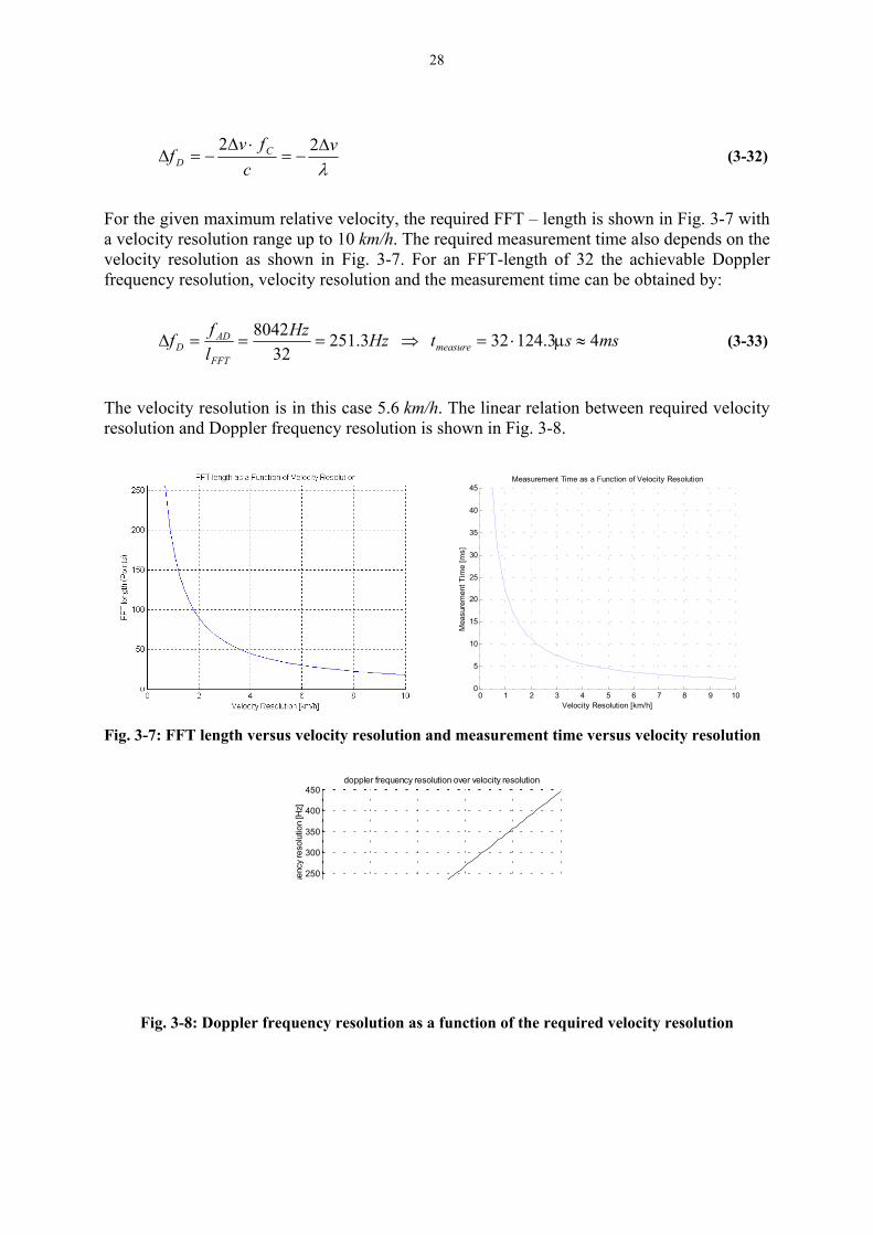
For the given maximum relative velocity, the required FFT – length is shown in Fig. 3-7 with a velocity resolution range up to 10 km/h. The required measurement time also depends on the velocity resolution as shown in Fig. 3-7. For an FFT-length of 32 the achievable Doppler frequency resolution, velocity resolution and the measurement time can be obtained by:

msstHzHzlff measureFFT

ADD 43.12432 3.251

328042

≈µ⋅=⇒===∆ (3-33)

The velocity resolution is in this case 5.6 km/h. The linear relation between required velocity resolution and Doppler frequency resolution is shown in Fig. 3-8.

0 1 2 3 4 5 6 7 8 9 100

5

10

15

20

25

30

35

40

45

Velocity Resolution [km/h]

Mea

sure

men

t Tim

e [m

s]

Measurement Time as a Function of Velocity Resolution

Fig. 3-7: FFT length versus velocity resolution and measurement time versus velocity resolution

250

300

350

400

450doppler frequency resolution over velocity resolution

uenc

y re

solu

tion

[Hz]

Fig. 3-8: Doppler frequency resolution as a function of the required velocity resolution

29

3.2.3.1 Processing with Stepped Ramps A concept with very short sweep voltage ramp signals of 124.3 µs duration over the complete range from 0 m up to 20 m for a maximum Doppler frequency of 8042 Hz is not possible due to the fact that the time per range gate is too short and the A/D-converter sampling frequency is high. A stepwise processing of the complete measurement range as shown in Fig. 3-9 seems to be better, but takes more time for a complete scan. The range is scanned using short ramps to sweep the sensor delay and only a few range gates are covered in a block-wise processing scheme. Fig. 3-9 shows a solution of eight steps to cover the complete range and only four range gates per step, i.e. 32 range gates over the complete range. This idea is a compromise between reduced calculation effort and a reduced range resolution which coincides with a reduced number of range gates. It is assumed that real targets will not only be seen in a single range gate, but are usually extended targets and distributed over more than one range gate.

Sweep Voltage [V]

measurement time [ms]

0.7

4.2FFT

32 ramps per step with 124.3µs each8 steps with 4 range gates in each one

4ms

2. step3. step4. step5. step6. step7. step

1. step8ms 12

Fig. 3-9: Processing with stepped ramps

For an A/D-converter sampling frequency of 8042 Hz per range gate and a Doppler frequency resolution of 124.3 Hz which corresponds to a relative velocity resolution of 5.6 km/h, 32 samples per range gate are required for the FFT. The resulting total A/D-converter sampling frequency is in this case:

(3-34) kHzHzf totalAD 168.328042432, =⋅=

With 4 range gates per short ramp and 8 consecutive steps of 32 short ramps per step, a total number of 32 range gates of same size are covered. With a total measurement range of 20 m the range gate size is:

cmcmRRG 52.6431

2000==∆ (3-35)

One measurement step covers .4.27752.644 cmcm =⋅The total measurement time for the complete range is:

(3-36) msst totalmeasure 82.313.124328, =⋅⋅= µ

30

That means within two cycles of 20ms each the velocity measurement of the complete range could be covered. The range gate size seems to be very large compared with the range resolution of the sensors, but it is a good compromise between computation effort and performance. Per velocity scan over the complete range only 32 FFTs of 32 complex values have to be calculated. The integration time per range gate for a single sample is in both cases:

sst µµ 1.3143.124

32int, ≈= (3-37)

3.2.3.2 Processing with Staggered Ramp Duration This chapter develops a new concept for velocity measurement using the described high range resolution pulse radar sensors. The main idea is to decrease measurement time by measuring velocity ambiguously. Range is measured unambiguously. So the concept is similar to an LPRF processing scheme with ambiguous velocity and unambiguous range measurement. In this special case the pulse repetition frequency is unchanged, but the duration of the sweep voltage ramp signals for the sensor is staggered in two different steps. Short Fourier transforms are then calculated for both different sections of ramp durations and ambiguities can finally be resolved by known algorithms like the Chinese remainder theorem. The resolution is a problem of number theory. Some solutions can be found in [ROH86] or [ROT90]. The basic principle of the sweep voltage applied in this concept is shown in Fig. 3-10.

Fig. 3-10: Processing with staggered ramp duration

It is obvious that with a ramp duration of e.g. 1 ms a maximum Doppler frequency of 1 kHz can be measured unambiguously. For the maximum values assumed above (180 km/h), the maximum Doppler frequency to be measured is 8042 Hz. To get unambiguous results the following processing scheme can be applied:

31

• Control of the sensor with voltage ramps of e.g. 1 ms (16 ramps) and accumulation of 16

samples for each range gate to be examined • Calculation of a short FFT only in relevant range gates for the collected samples yields

Doppler spectrum 1 • Detection in Doppler spectrum 1 by application of an adaptive threshold algorithm (e.g.

OS-CFAR) • Control of the sensor with voltage ramps of e.g. 700 µs (16 ramps) and accumulation of 16

samples for each range gate to be examined • Calculation of a short FFT only in relevant range gates for the collected samples yields

Doppler spectrum 2 • Detection in Doppler spectrum 2 by application of an adaptive threshold algorithm (e.g.

OS-CFAR) • The two received Doppler values for a target within a range gate are ambiguous. ⇒ Resolution of Doppler frequency ambiguity. The results are the Doppler frequencies

of the target detected in the range gate. To reduce the number of FFTs to be calculated the samples can be examined before a transform to find out relevant range gates including real targets. Example: For a short example the following values are selected: • Duration of ramp 1: msTR 11 =• Duration of ramp 2: sTR µ7002 =The sensor is controlled by 32 ramps, 16 of each of both types. So the complete time for one cycle is:

(3-38) mssmstcycle 2.2770016116 =⋅+⋅= µ

The sampling frequency under the assumption that 32 range gates are sampled is: • for the 1st part with ramps of 1 ms: 32.0 kHz • for the 2nd part with ramps of 700 µs: 45.714 kHz The resulting sampling frequency for each range gate is: • for the 1st part with ramps of 1 ms: 1.0 kHz • for the 2nd part with ramps of 700 µs: 1.43 kHz For a Doppler frequency of for example 3.2 kHz, the measured frequencies are e.g. 0.2 kHz and 0.34 kHz respectively. These frequencies can be continued with the sampling frequency, because this is the frequency range of the FFT. The result is: • ramp 1: 0.2kHz (1.2kHz 2.2kHz 3.2kHz) • ramp 2: 0.34kHz (1.77kHz 3.2kHz) If in each of both series the same Doppler frequency is found, the corresponding frequency is the result of the ambiguity resolution algorithm. Some ideas how these ambiguities can be resolved are described in the Appendix. With an FFT of length 16 the Doppler frequency resolution and the velocity resolution can be calculated for both parts:

32

• ramp 1: HzkHzlf

fFFT

AD 5.6216

1===∆

hkm

sm

fcfv

C

4.139.02

==⋅∆

=∆ (3-39)

• ramp 2: HzkHzlf

fFFT

AD 8916

43.1===∆

hkm

sm

fcfv

C

255.02

==⋅∆

=∆ (3-40)

It can be seen that a high velocity resolution can also be achieved with this method although the measurement time and the A/D-converter sampling frequency are acceptable low. Comprehension of the concept: • low sampling frequency of A/D-converter • short length of FFT to be calculated • high achievable Doppler frequency and velocity resolution • By resolution of ambiguities the velocity range that is covered by this concept is very high,

although the sampling frequency stays low enough to manage A/D-conversion with commercial ICs

• It is not expected to have more than one or two obstacles in each range gate. Multi-target situations can generate wrong velocities in the resolution of ambiguities, but a tracking algorithm can check the result for plausibility and find out wrong results easily.

• The estimated velocity by measuring a range rate can be used as an additional information for the resolution of ambiguities.

Resolution algorithms for range and Doppler ambiguities are mentioned in [ROH86]. These algorithms can be transformed to the resolution problem of Doppler ambiguities in this chapter. The easiest approach to this problem is the Chinese remainder theorem [SCH90]. It finds solutions for natural numbers. A modified algorithm described in the appendix also finds solutions for real numbers. One possible single-target situation is shown in Fig. 3-11.

Fig. 3-11: Doppler frequency resolution

To measure the two ambiguous frequencies two different ramp frequencies have to be used for sensor control. The two ramp frequencies are smaller than the maximum Doppler frequency. For the measured frequencies M1

’ and M2’ which differ from each other, the true

Doppler frequency of the detected single object has to be determined by expanding the

33

frequency scale for both ramps. The value where both expanded frequencies are equal is the true Doppler frequency of the detected object:

(3-41) '222

'111 MfVMfVM +⋅=+⋅=

With the division of both frequency intervals f1 and f2 into J1 and J2 subsections the resulting unambiguous range for the Doppler frequency is:

(3-42) 1221max, JfJff D ⋅=⋅=

In Fig. 3-11 the solution is V1=7 and V2=8. See Appendix for a detailed description of the algorithm for resolution of ambiguities.

3.3 Variable Pulse Width The very high range resolution which can be achieved with a radar using ultra-short pulses is not always desired. For the very near range the received energy is sufficient for detection, and high range resolution makes sense. On the other hand received energy of targets at 20 m is significantly reduced and high range resolution is of minor interest in this situation. Safe detection also of small reflectors at 20 m is important and also high range accuracy, but not resolution. The intention of this chapter is to show effects of sensor transmit pulse width variations on other parameters influencing the system performance. Several questions rise when discussing this topic. The questions are followed by possible solutions and answers always under consideration of practical feasibility and approaches to find a suitable solution for transmit pulse width variation. The most important sensor features to be considered are listed in Table 3-1.

3.3.1 Parameters for Variable Range Resolution The achievable range resolution in pulse radar systems depends on the pulse width. The simple relation between range resolution and pulse width TP is:

cmssmTc

R p 6104001035.02

128 =⋅⋅⋅⋅=⋅

=∆ − (3-43)

An assumed pulse width of 400 ps results in a theoretical range resolution of 6 cm. For FMCW-radars the comparable parameter bandwidth is the key parameter for range resolution. The relation between range resolution and transmit signal bandwidth is:

Hubf

cR⋅

=∆2

(3-44)

34

For a range resolution compared with the value of the pulse radar calculated above (6 cm), the required frequency hub is 2.5 GHz. Fig. 3-12 shows resulting range resolution versus transmit signal pulse width using a pulse radar and also versus frequency hub when using an FMCW radar.

500 1000 1500 2000 2500 30000

5

10

15

20

25

30

35

40

45

Pulse Width [ps]

Ran

ge R

esol

utio

n [c

m]

Range Resolution as a Function of Pulse Width

0 500 1000 1500 2000 2500 3000 35000

5

10

15

20

25

30

35

40

45

Frequency Hub [MHz]

Ran

ge R

esol

utio

n [c

m]

Range Resolution as a Function of Frequency Hub

Fig. 3-12: Range Resolution as a Function of Pulse Width and Frequency Hub

3.3.2 Influences of Variable Pulse Width on the System Performance The variation of the transmit pulse width influences different magnitudes which have to be considered in order to decide which time range is the optimum for pulse width variation. The influenced parameters are: • Range resolution • Time on target • Average transmit power • Signal to noise ratio • Probability of detection and probability of false alarms • Sensor to sensor interference (probability of false alarms due to interference) The influences of pulse width variation on the specific parameters will now be discussed. Range resolution: The influence on target range resolution is shown in Fig. 3-12. In this case the pulse width was increased from the achievable pulse width of 400 ps with range resolution of 6 cm up to 3 ns resulting in a range resolution of 45 cm. In general very high range resolution makes sense for applications up to 5 m while for distances of more than 5 m reduced resolution of e.g. up to 40 cm at 20 m may be sufficient. Additionally the received energy increases which is required to detect small targets at distances of more than 5 m (e.g. safe detection of a person up to 10 m). The duty cycle is the ratio between pulse width and the length of a PRI (pulse repetition interval). In both mentioned cases (400 ps and 3 ns) with a pulse repetition frequency of 4 MHz the duty cycles are:

35

400 ps → 0.16% duty cycle 3 ns → 1.2% duty cycle

PRI

P

TT

= cycleduty (3-45)

Time on target / average transmit power: The increase of duty cycle from 0.16% up to 1.2% is equivalent with an increase of time on target by a factor of 7.5 in our example. Average transmit power is assumed to be proportional to the duty cycle. Thus the increase of average transmit power will also be achieved by a factor of 7.5. The peak power is assumed to remain unchanged. 400 ps → -19 dBm (12.6 µW) 3 ns → -10.2 dBm (94.4 µW)

with: (3-46) [ ] [( mWPdBmP log10 ⋅= ]) The average transmit power can be expressed as the transmitted energy per PRI and the transmitted energy per interval is the integration of the pulse power per pulse repetition interval.

PRI

PRIavg T

EP = ; ⇒ ( )∫ ⋅==PRIT

PpeakPRI TPdttPE0 PRI

Ppeakavg T

TPP ⋅= (3-47)

Difference between coherent and non-coherent integration: Integration of signals within the receiver is separated into coherent and non-coherent integration. It is clear that the signal-to-noise ratio can be increased by integration of numerous pulses in a pulse radar. Integration is often necessary due to the very small energy of single pulses, especially in pulse radar systems with very high range resolution, i.e. very short pulses. Coherent and non-coherent integration have different influences on the increase of signal-to-noise. Coherent integration means that all pulses to be integrated have the same signal phase. The so-called SNR-improvement can be expressed as follows for a coherent integration:

( )( ) n

NSNS

I nSNR ==

1

(3-48)

The signal-to-noise is increased by a factor of n if n pulses are integrated in the receiver. This is the best SNR-improvement that can be reached with the disadvantage that a coherent integrator requires additional hardware and cost. Non-coherent integration is a direct integration of pulses without using the phase information. In the case of the HRR radar a non-coherent integration is performed with the following SNR-improvement:

36

with . (3-49) γnI effSNR =, 1<γ

The number of integrated pulses depends on the time on target which is in our case a function of the slope of the sensor delay sweep. Signal-to-noise ratio: From the radar equation (see Appendix) the relation between signal-to-noise ratio and pulse width can be formed:

( )( )

( Ptatmtnsys

Paus

TPLLBkTR

GTNS

⋅⋅

⋅⋅⋅

=

1

4 43

22

πσλ ) (3-50)

The signal-to-noise ratio depends directly on the transmitted power which is the only variable in the radar equation that depends on the pulse width TP. With the transmitted power expressed as the average power being a function of the pulse width, the radar equation gets:

( )Pt TP

( )( ) P

PRI

Ppeak

atmtnsysP

aus

TKTTP

LLBkTRGT

NS

⋅=⋅⋅⋅

⋅⋅⋅

=

1

4 43

22

πσλ (3-51)

This is still the signal-to-noise ratio with consideration of only a single pulse. Non-coherent integration increases the signal-to-noise ratio after integration of n pulses:

( ) ( ) Pn TKnnNSNS ⋅⋅=⋅= γγ1 (3-52)

Probability of detection (PD) and probability of false alarms (PFA): The probability of detection is a function of the signal-to-noise ratio. A short derivation of the probability density functions (PDF) of the envelope of signal plus noise and noise only can be found in the Appendix. Having the PDFs, the probability of detection and the probability of false alarms can be derived by integration of the PDFs. The probability of false alarms depends on the noise variance and on the detection threshold:

−=

−= ∫

∞

222 2exp

2exp

N

T

V NNFA

VdrrrPT

σσσ (3-53)

The probability of detection can also be calculated by integration of the Rician PDF:

( ) ∫∫∞∞

⋅⋅

+−==

TT V NNNVriceD drr

NSI

NSrrdrrpP

σσσ2

2exp 02

2

2 (3-54)

37

DP is a function of the signal-to-noise ratio and the detection threshold VT. The integral shown above can only be solved numerically. It was shown above that the signal-to-noise ratio increases linearly with an increase of the transmit pulse length at constant target range R. The integral for the probability of detection can not be solved easily, but often diagrams are used to show the signal-to-noise as a function of the probability of detection (see Fig. 3-13).

Fig. 3-13: SNR versus PD for single pulse detection (Source: [LEV88])

Sensor to sensor interference: With longer pulses the probability of sensor to sensor interference increases. It is of interest how the false alarm rate increases with longer transmit pulse length. This will be discussed in the next chapters. To understand the effect of interference, some important explanations and possible solutions assuming constant pulse length are given.

3.3.3 Example for Pulse Width Variation It was already explained that the signal-to-noise ratio as the key parameter for target detection increases linearly with linear increasing pulse width at constant target range R. The S/N decreases fast with increasing range R:

( ) PP TR

factorTRNS

⋅⋅= 4

1, (3-55)

38

To keep the signal-to noise ratio at an acceptable level for a moving target, the pulse width should be changed non-linear. A quadratic increase with range R can be a good solution (see Fig. 3-14):

( )2

min,max,min, 20

⋅−+=

mRTTTT PPPP (3-56)

0 2 4 6 8 10 12 14 16 18 200

0.5

1

1.5

2

2.5

3

Distance [m]

Pul

se W

idth

[ns]

Transmit Pulse Width vs. Distance

0 2 4 6 8 10 12 14 16 18 201

2

3

4

5

6

7

8

Distance [m]

Incr

ease

of S

igna

l-to-

Noi

se ra

tio

Signal-to-Noise increase: S/N(wider pulse) to S/N(normal)

Fig. 3-14: Transmit pulse width versus distance and increase of signal-to-noise ratio versus

distance

3.4 Suppression of Sensor Interferences It is known from pulse radars that two of them transmitting in the same frequency band can very well interfere each other. This effect can also be observed when using the described high range resolution pulse radar sensors in a sensor network installed into a vehicle bumper. The distance between the sensors is small compared with the maximum measurement range and interferences between the sensors can be observed. These may be caused by reflections behind the vehicle bumper and also when a strong reflector is close to the vehicle. This chapter gives important explanations concerning the origin of interferences and reveals some ideas how to avoid interferences.

3.4.1 Explanation of Sensor Interference An example of sensor interference is shown in Fig. 3-15 in order to see which issues are caused without any suppression of sensor interference and to understand how necessary it is to avoid this effect. The target distances of a single sensor target list are shown versus time. The situation was an approaching and receding experimental car to the back of another vehicle which was detected very well. The steep lines indicate that interfering pulses from other radars were also integrated resulting in artificial target peaks in the sensor IF signal. It is clear that interference renders correct data association and therefore precise angle estimation and also measurements with low false alarm rate very difficult. In realistic street situations the probability that two sensors report a detection caused by sensor interference at the same time and at a very similar range was observed to be very low.

39

That means that in most cases the tracker deletes the false targets of a single sensor and avoids false objects in the object map. Nevertheless interference is an unwanted effect that may also cause false tracker outputs and increases computation complexity for the single sensor tracker.

Fig. 3-15: Example of sensor interference

To understand the phenomenon of interference, Fig. 3-16 shows the transmit and receive pulses for a single target situation with a target at 15 m distance to all sensors (delay time 100 ns). The small difference of delay time and distance between each other is neglected. Receive pulses are marked by smaller amplitude. A pulse repetition frequency of 4 MHz was assumed. That is a total unambiguous range interval of 37.5 m. Further it is assumed that the PRF generators are not synchronized and the delay between each other is chosen randomly.

0 ns= 0 m

250 ns= 37.5 m

133 ns= 20 m

Amplitude

Time

S1

S2

S3

S4

Fig. 3-16: Transmit and receive pulses of four sensors

40

Fig. 3-16 shows that receive pulses of sensors S2...S4 are of course also received by sensor S1. If a sweep signal of 15 ms duration is applied, the time per range gate is approximately 58.8 µs. In each range gate 235 pulses will be integrated. For a strong reflector, the integrated pulses received by other sensors than sensor S1 at a constant range (delay) form a peak in the IF signal. If the pulse repetition frequencies of the sensors are very constant and all precisely 4 MHz, much energy from other sensor’s pulses can be integrated and a peak in the IF signal can be observed. If the PRFs differ from each other by a specific minimum frequency, the received pulses of e.g. sensor S2 within consecutive pulse repetition intervals are found in different range gates of e.g. sensor S1 within consecutive PRIs. So not many pulses will be integrated by sensor S1 and no artificial target will be detected in the sensor S1 IF signal. On the other hand sensor S2 receives its own pulses all in the same range gate in consecutive PRIs and received pulses from sensor S1 are not all integrated in the same range gate in consecutive PRIs. So no artificial target will be detected due to sensor S1 transmit pulses received by sensor S2. The minimum value for the difference of the PRF between two sensors will be calculated later. The lines of detections crossing the diagram Fig. 3-15 can be explained using the illustrations of Fig. 3-16. By zooming into the picture, it can be seen that in a time period of approximately 6 cycles (120 ms) and probably multiples of 250 ns a peak in Fig. 3-15 crosses the complete range from 20 m down to 0 m. From this information the difference of the PRF of the interfering sensor to the shown sensor can be calculated. A range of 20 m corresponds to a time delay of 133 ns. For a single cycle of 20 ms a delay of

6

133250 nsnskTcycle −⋅=∆ ; with k unknown (3-57)

can be calculated between the two PRFs. For 1 s the time is

−⋅⋅=∆

6133250501

nsnskT s (3-58)

i.e. for one PRF cycle of 250 ns the difference in time is:

61041

613325050

⋅⋅

−⋅⋅=∆ −

nsnskT cyclePRF (3-59)

So the difference in PRF between the two oscillators is (under the assumption that one of them has a PRF of exactly 4 MHz):

⋅−⋅⋅⋅+

⋅−=∆−

−

61013310250501

1449

9kMHzMHzf (3-60)

41

In the case that two PRF oscillators trigger the transmit switches with exactly the same frequency, a false target (caused by received pulses from another sensor) with constant distance to the real target distance would be observed. With a small difference between the PRF oscillator frequencies the false target is moving. With bigger difference of both PRFs the probability of false alarms caused by another sensor is significantly reduced. There are three cases to be distinguished for the analysis of false alarm rate caused by sensor interference. These are:

1. PRFs of two sensors are absolutely identical 2. PRFs differ very strong from each other 3. PRFs are very similar to each other

These cases will now be discussed in detail: 1. PRFs of two sensors are absolutely identical This case is unrealistic because the reproducibility of two oscillators can not be done in such a precise manner that the frequencies are absolutely identical. Each reflected transmit pulse of sensor S1 would be integrated by sensor S2. Therefore the false alarm rate only depends on the target size and can be calculated using the radar equation. For a reflector of big radar cross section the probability of false alarms tends to one. 2. PRFs differ very strong from each other This case occurs if the following difference for the PRFs of two sensors is observed:

cyclePRFTns

MHzf−∆−

−=∆250

14 with: (3-61) PcyclePRF TT >∆ −

This is also the criterion for interference suppression with constant detuning of the PRF oscillator, i.e. in this case the probability of false alarms tends to zero, because only a single pulse per PRI might be integrated in the same range gate. This criterion assures that the reflected pulse changes the range gate in consecutive PRIs. 3. PRFs are very similar to each other For this case where the resulting false alarm rate depends on the target radar cross section and on the difference of the two PRFs, the following criterion must be met:

cyclePRFTns

MHzf−∆−

−=∆250

14 with: (3-62) PcyclePRF TT <∆ −

For this case with slightly detuned PRF oscillators the probability of a false alarm is somewhere between zero and one.

3.4.2 Constant Detuning of the PRF Oscillator One way for interference suppression can be to vary the PRF oscillator frequencies of individual sensors. In this case the difference has to be big enough to avoid integration of

42

receive pulses of a second sensor. The time difference in consecutive PRIs has to be at least one pulse length:

(3-63) psT cyclePRF 400>∆ −

The resulting difference in frequency under the assumption that one sensor is triggered with 4 MHz is:

kHzTns

MHzfcyclePRF

41.6250

14 =∆−

−=∆−

(3-64)

0 ns 250 ns

Amplitude

Time

S1

S2

500 ns 750 ns

PRF1 = 4 MHz PRF2 = 4 MHz + ∆f

Fig. 3-17: PRF-oscillator detuning for interference suppression

Fig. 3-17 shows the situation with the difference of two PRFs being 6.41 kHz. For a smaller difference, integration of consecutive pulses will not be absolutely avoided, but the amplitude of interference peaks in the IF signal can be reduced, i.e. the probability of false alarms due to interference is reduced. To maintain unambiguity of range measurement, the PRF should not be increased too much. For the example of ∆f = 6.41 kHz (400 ps difference) the unambiguous range for distance measurement decreases only by 6 cm which is the range resolution for the chosen pulse width of 400 ps. It is also possible to vary the PRF slowly depending e.g. on the DSP time counter since system start. It must be avoided that two cars equipped with the system run the same frequency pattern for PRF oscillator detuning. A random variation of the PRF explained in the next subchapter can be a safer solution. [MEI01] suggests to vary the transmit signal depending on the driving direction of the car to avoid interferences.

3.4.3 Jittering of the Pulse Repetition Frequency A pseudo-noise like variation of the PRFs can be one solution to exclude that two sensors whose PRFs are changed during the measurement process run the same frequency pattern. This can be accomplished by delaying the minimum time of one PRI (e.g. 250 ns at 4 MHz PRF) by an additional time of uniform distribution up to a maximum time. The maximum time has to be set in order to ensure that within one scan cycle of the sensor (e.g. 20 ms) enough pulses will be integrated to form a detectable peak in the IF signal. The distribution of

43

a pseudo-noise like PRF delay time is a uniform distribution and the probability density function is a constant with amplitude 1/∆T from 0 up to ∆T. ∆T should not be larger than e.g. 0.1⋅PRI (in our case 25 ns, ) to keep reduction of amplitude due to less energy that will be integrated as small as necessary.

kHzf 363max ≈∆

It depends on the specific hardware whether it is possible to change the PRF after each PRI which should be preferred or to change the PRF after one complete measurement cycle. If latter is the only way, it might still be possible that false alarms occur in a single cycle if two sensors have nearly the same PRF during one measurement cycle of 20 ms, but the probability for this case is very low. Furthermore it must be checked how the PRF can be changed, continuously or in discrete frequency steps. For one sensor the probability that the PRI delay time equals a specific time T1 up to T1 + TP is:

( ) ∫+

∆=

∆=+<<

PTT

T

PPS T

TdT

TTTP1

1

111111 ττ (3-65)

This is the same for a second sensor and if both statistic independent results are combined the probability that two sensors have the same PRI delay with discrete size TP is:

( )T

TTTTTTTPP PPPerfere ∆

=+<<+<<= 121111int , ττ (3-66)

For our case with ∆T = 25 ns and TP = 400 ps the probability is:

(3-67) 016.0400,int =pserfereP

With additional application of pulse width variation up to pulses of 3 ns the probability of interference increases

⇒ 12.03,int =nserfereP 5.7400,int

3,int =pserfere

nserfere

PP

(3-68)

This is the probability that a false alarm occurs in the case that the PRF is only changed every measurement cycle (e.g. 20 ms). This should be low enough to decide that a change every cycle is sufficient under the aspect that additionally the tracker eliminates such false alarms easily. To give a number, the probability that in at least L out of M cases a false alarm occurs due to interference is:

∑=

−

∆−⋅

∆⋅

=

16

8, 1

L

LMPulse

LPulse

trackFA TT

TT

LM

P (3-69)

44

e.g. for M = 16 and L = 8: and P 11400,, 1093.4 −⋅=pstrackFAP 4

3,, 10256.2 −⋅=nstrackFA

If the PRF is changed with each new pulse and with only a few discrete frequency steps for the PRF, the probability of a false alarm is much lower and the probability of a false track tends to zero. Major advantages of a change of the PRF after each single pulse are a reduced probability of false alarms and the possibility to avoid ambiguities in range measurement which may occur if the pulse width is changed for measurements at long distances to achieve a higher signal-to-noise ratio.

45

4 Radar Network Processing The introduction of radar data fusion techniques for this specific application is very new and requires special topics to be considered, because target detection in the extreme short range of vehicles and fusion of this target data obtained with very high range resolution pulse radars was never considered before. Especially the very dynamic surrounding of a moving vehicle in normal street or highway traffic situations is a very difficult challenge. To cope with data fusion and filtering techniques in the sensor network is the topic of this chapter. In this case practical feasibility with limited processing power at high update rate will be an important aspect to keep the system as cheap and simple as possible, but also more sophisticated methods (e.g. multiple hypotheses tracking) will be taken under consideration in order to achieve better performance. It is in fact a very special case that the sensor measurements only consist of range information of high accuracy and resolution. Additional amplitude information may help in some cases of data association. To understand the explanations in this chapter it is first necessary to define the following expressions: Target: A target is the obstacle that is in a sensor’s field of view. Target List: The target list is the set of targets detected in one cycle including information

for each single target. This set including target range, amplitude and velocity (if measured) is transmitted from each sensor’s digital signal processor to a central processor (radar decision unit: RDU).

Intersection: An intersection is an estimated object position for the current measurement cycle. It is calculated by associated target ranges from the network sensors to the real obstacle. Two, three or four target ranges may contribute to one intersection.

Object: An object is the result of the data fusion process. It is obtained by tracked intersections and described by its Cartesian position coordinates and its Cartesian velocity components.

Object Map: The object map is the system output and the relevant information for a following application processor.

4.1 Coordinate System For tracking and data fusion algorithms in an automotive radar network two different coordinate systems can be defined. On the one hand the use of a polar coordinate system makes sense, because measured quantities of radar sensors are usually output in polar coordinates, i.e. range and if possible angle and radial velocity. A transformation to another coordinate system would not be necessary in this case, but many operations of tracking algorithms would use trigonometric expressions. This is very time-consuming for the tracking processor. The selection of a Cartesian coordinate system implies a transformation of measured quantities to the Cartesian coordinate system. This step is performed in the system modelling where non-linear measurement equations are linearized. It is done as well in non-linear least squares estimation as in the Kalman algorithms described in this work. Coordinate definitions for a system integrated into a vehicle front bumper are given in Fig. 4-1. For a vehicle consisting of additional subsystems in the rear bumper and on the sides it is a good solution to use coordinate systems for each subsystem separately and relate all results to a common coordinate system with its origin in the vehicle center. In this case the adaptive cruise control and safety algorithms get all data related to one common origin of all

46

subsystems. It showed to be very easy to use the same tracking algorithms for all subsystems only with different sensor locations for each individual subsystem.

vx,car

vy,car

αobj

x

y

vx,obj

vy,obj

z

(xobj,yobj)

robj

Fig. 4-1: Coordinate system

Additionally automotive radar applications show in most cases objects moving along the vehicle symmetry axis or perpendicular to it. So to track in Cartesian coordinates shows advantages compared with polar coordinates. Automotive radar systems usually track in two dimensions, because height measurement is difficult or impossible with nearly all existing systems.

4.2 Multiple Sensor Network Architectures In the following chapters some possible architectures for an automotive sensor network are compared. It has to be distinguished between the hardware structure with separate control units and communication wires and the signal processing structure determining which parts of the complete signal processing and tracking will be performed in the specific elements of the network. [BLA99] proposes some architectures divided into central-level tracking and sensor-level tracking which will be discussed in the following sections under the aspects of an automotive radar sensor network.

4.2.1 Network Architectures The first possible hardware architecture is shown in Fig. 4-2. In this case all sensors are directly connected to a central ECU (electronic control unit) or RDU which is the single processor in the system. The ECU controls all sensors and converts all analog sensor output signals to digital data in parallel for further processing by a DSP. It is always preferable to contain all important information in a single unit, but the processor load is too high for all necessary peripheral tasks and the complete detection, data association, estimation and tracking algorithms. Additionally the wires between the sensors and the ECU should be short, because external noise (e.g. ignition sparks causing electromagnetic compatibility issues) can

47

reduce the signal-to-noise ratio. On the other hand there is no performance degradation by latency (delay for digital data transmission).

Sensor 1Sensor 2 Sensor 3

Sensor 4

Radar decision unit

analog 1 analog 2 analog 3 analog 4

CAN

Sensor-DSP &

Application

Fig. 4-2: System architecture 1

The second possible architecture uses separate signal processing hardware for each sensor to control the individual sensor and to sample and convert the sensor output signals to a digital data stream (Fig. 4-3). Included detection algorithms process the sensor output and the individual processors transfer information to a central processor. The used sensor processors can also be used for sensor self-calibration if located inside the sensor package. In this case a single sensor is a compact unit with a digital serial field bus interface (e.g. a CAN bus) to communicate with other processors. From an analog signal, the remaining information to be transmitted is significantly reduced to a list of observations.

Sensor 1Sensor 2 Sensor 3

Sensor 4

DSP 1 DSP 2 DSP 3 DSP 4

Radar decision unitCAN 1

CAN 2 CAN 3

CAN 4

CAN

Application

Fig. 4-3: System architecture 2

A system with distributed processing has the disadvantage that latency has to be considered in the data fusion and tracking algorithms. Synchronization of the network has to be managed by the central radar decision unit. Synchronization via CAN bus messages on separated buses was recognized to be not feasible in this system due to delay times between digital data transmission. The best solution is a prioritised interrupt line from the radar decision unit to the sensors, so that all sensors start their range sweep at the same time. Triggered by the radar

48

decision unit e.g. every 30 seconds, the sensors can be re-synchronized and drift can be avoided. For data transmission the four sensors can also be connected to a single bus rather than using separated buses. This depends on the amount of data to be transmitted and on the maximum bus load.

4.2.2 Software Architecture: Central-Level Tracking Assuming the network hardware structure to be as shown in Fig. 4-3 all sensors have an own signal processing unit to preprocess the sensor output signals. The information flow between the sensors and the RDU is reduced to a list of observations (detections of true targets and false alarms). For each cycle a complete new shot of the situation is taken and a new list of observations is transmitted untracked to the radar decision unit. The RDU performs the following necessary tasks like data association and update of the estimated target states, gate calculation for the data association and also an initiation of new tracks (see Fig. 4-4). Obviously the sensors do not communicate between each other. All data is collected in the RDU to perform a data fusion. [BLA99] also suggests a central-level tracking with partitioned processing. This structure differs from Fig. 4-4 in the following points. A local data association is already performed in the single sensor processor considering the calculated gating information received from the RDU. Associations and remaining observations of all sensors are then transmitted to the RDU. The remaining observations are further used for the initiation of new tracks and the associations are directly considered for the global track update.

ObservationsSensor 1

ObservationsSensor 4

GlobalAssociation

TrackInitiation

GlobalTrack Update

GateCalculation

ObservationsSensor 2

ObservationsSensor 3

Fig. 4-4: Central-level tracking with centralized processing

For the system considered in this work a centralised processing is preferred in comparison with a partitioned processing due to the fact that the additional effort to be spent for the data association in the RDU is less than the effort needed for the increase in data amount to be transferred. It is the better way to concentrate as much of the processing in the central RDU as possible.

4.2.3 Software Architecture: Sensor-Level Tracking Compared to a central-level tracking a sensor-level tracking already performs target tracking within each sensor unit. As Fig. 4-5 shows, local sensor observations are associated to local tracks or local tracks are initiated by local data. Local track information can then be used for

49

local data association adaptive gate calculation. Local track data of all sensors performing a sensor-level tracking is then transmitted to a central processing unit for central track data fusion. Track to track association methods are necessary in the central processor to initiate and update global tracks. Sensor-level tracking reduces complexity in the RDU and data transmission between RDU and sensors.

Local DataAssociation

TrackInitiation

LocalTrack Update

GateCalculation

Local Observ.Sensor 1

GlobalAssociation

GlobalTrack Update

OtherSensors

Tracks

Fig. 4-5: Sensor-level tracking with centralized track file

Also for sensor-level tracking the distributed track file method is possible. This would look like Fig. 4-5 with global track to track association and global track initiation and update performed in each single sensor unit. In this case the interfaces between the sensors are used to transmit local track information of each sensor to all other sensors. With this strategy all sensors have all local track information of other sensors available and calculate their own representation of the situation. This involves much redundancy in the system and higher computation complexity in each single sensor unit. Distribution of track files makes the system robust and flexible because it has no central processing unit. To draw a conclusion of the possible processing structures it should be noted that sensor-level tracking can be important for networks consisting of many individual sensors. In a network of four sensors central-level tracking with centralized processing should be preferred. This is also the structure of the network described in this thesis.

4.3 Single Object Multilateration and Tracking Under the assumption that only a single object has to be tracked by the radar network, the following pages show basic tracking algorithms and their properties in a radar network. From this simple case the handling of multiple objects will be the following step. The least squares estimation ([LAY97]) as well as the Kalman filter are designed to calculate object positions from range measurements only.

50

4.3.1 Nonlinear Least Squares Estimation With two measured ranges the object position can be calculated as the intersection of two circles around the two sensors with the radius being the measured range. With three and even four measured ranges a nonlinear least squares position solution can be calculated to make use of the given redundancy and to find a more precise solution. An example of such a situation is given in Fig. 4-6. Four sensors measure different target ranges in this situation and each sensor is assumed to include a range error. This may be a systematic error, e.g. in the case that the sensor positions in the bumper are only known with limited precision. Another systematic range error depending on the target range is the remaining range measurement error of a sensor for which an absolute maximum value of 3 cm is assumed. Stochastic errors can be seen e.g. in slightly different backscatterer positions on the reflecting object due to different aspect ratios from the individual sensors.

r1 r2 r4r3

Sensor 1Sensor 2 Sensor 3

Sensor 4

estimated least squaresobject position

xy

Fig. 4-6: Example of an estimated object position by means of a least squares algorithm

This chapter shows an iterative approximation algorithm to find an optimal position solution based on least squares estimation:

Assume that the object position to be estimated is denoted as: (4-1)

=

t

t

yx

tr

The four sensor position coordinates for the sensors s1..4 related to the center of the front bumper are:

=

1

11

s

s

yx

sr (4-2)

=

2

22

s

s

yx

sr

=

3

33

s

s

yx

sr

=

4

44

s

s

yx

sr

The four differences between the sensors and the object are further denoted as:

Sensor 1: l Sensor 2: l

−−

=−=ts

ts

yyxx

ts1

111

rrr

−−

=−=ts

ts

yyxx

ts2

222

rrr

51

Sensor 3: l Sensor 4: l

−−

=−=ts

ts

yyxx

ts3

333

rrr

−−

=−=ts

ts

yyxx

ts4

444

rrr

(4-3)

For the nonlinear equations we get:

( ) ( )( ) ( )( ) ( )( ) ( ) 4

24

244

32

32

33

22

22

22

12

12

11

nyyxxr

nyyxxr

nyyxxr

nyyxxr

tstsm

tstsm

tstsm

tstsm

+−+−=

+−+−=

+−+−=

+−+−=

(4-4)

with being the measured distances between the object and the sensors while n4...1, =irmi i describes the additive noise parts. We see that the relationship between the measured distances and the object states to be estimated is nonlinear. The measurement equation from above is:

(4-5) ( ) nxhz rrr+=

with being the vector of measurements, is the nonlinear function of the states and the measurement noise vector.

zr ( )xhr

nr

The noise parts are assumed to be independent and the noise covariance matrix R is:

(4-6) [ ]

=⋅=

24

23

22

21

000000000000

σσ

σσ

TnnER rr

The nonlinear equations can be linearized near an estimated solution using the method of Newton-Kantorowitsch (see [BRO]):

Using an estimated position denoted as: (4-7)

= )0(

)0()0(

t

t

yxt

r

the linearization becomes:

( )( ) ( ) ( )

( ) ( ) ( )eFyyy

rxx

xr

rr tttt

mitt

tt

mimimi +−

∂∂

+−∂∂

+= )0()0(

)0()0(

)0(

)0()0( rr

(4-8)

Neglecting the higher order error term F(e) the linearized equations are as follows:

52

xHz r̂r∆⋅=∆ ⇔

( )( )

( )( )

( )( )

( )( )

( )( )

( )( )

( )( )

( )( )

−−

⋅

∂∂

∂∂

∂∂

∂∂

∂∂

∂∂

∂∂

∂∂

=

−−−−

)0(

)0(

)0(4

)0(4

)0(3

)0(3

)0(2

)0(2

)0(1

)0(1

)0(44

)0(33

)0(22

)0(11

)0()0(

)0()0(

)0()0(

)0()0(

tt

tt

tt

m

tt

m

tt

m

tt

m

tt

m

tt

m

tt

m

tt

m

mm

mm

mm

mm

yyxx

yr

xr

yr

xr

yr

xr

yr

xr

rrrrrrrr

rr

rr

rr

rr

(4-9)

( )( ) ( )

( )( ) ( )

( )( ) ( )

( )( ) ( )

( )( ) ( )

( )( ) ( )

( )( ) ( )

( )( ) ( )

43421

44444444444 344444444444 21

43421r

r

x

tt

tt

H

tsts

ts

tsts

ts

tsts

ts

tsts

ts

tsts

ts

tsts

ts

tsts

ts

tsts

ts

z

mm

mm

mm

mm

yyxx

yyxx

yy

yyxx

xxyyxx

yy

yyxx

xxyyxx

yy

yyxx

xxyyxx

yy

yyxx

xx

rrrrrrrr

ˆ

)0(

)0(

24

24

42

42

4

4

23

23

32

32

3

3

22

22

22

22

2

2

21

21

12

12

1

1

)0(44

)0(33

)0(22

)0(11

∆

∆

−−

⋅

−+−

−−

−+−

−−

−+−

−−

−+−

−−

−+−

−−

−+−

−−

−+−

−−

−+−

−−

=

−−−−

(4-10)

)0(

mir is the distance between the estimated position t and sensor i. The measurement residual vector is the difference between the actual measurements and the expected measurements . is the estimated object position error. Matrix H is the measurement matrix.

)0(r

zr∆)0(

mir x̂r∆

The least squares solution of the system of linearized equations can be obtained by minimization of a weighted sum of squares of deviations (see also [BLA99]):

0ˆ =∆∂∂

xJr with: ) (4-11) ( ) ( xHzRxHzJ

T ˆˆ 1 rrrr∆−∆∆−∆= −

The solution is finally:

(4-12) ( ) zRHHRHx TT rr∆⋅⋅=∆ −−− 111ˆ

Assuming that all sensors show similar noise (4.12) can be simplified to:

(4-13) ( ) zHHHx TT rr∆⋅=∆

−1ˆ

Summarized the iteration steps are:

53

1. Assume an initial position to start the iteration. To ensure that the solution of the iteration converges the wanted solution the initial value has to be chosen near the expected solution.

2. Calculation of the linearized system of equations (matrix H). 3. Calculation of the estimated position error. 4. Correction of the selected starting position with the obtained error vector . x̂r∆5. Restart iteration if not yet converged. With remaining errors being very small,

convergence is usually reached after four iterations. The iteration can be aborted if a fixed convergence threshold ε is reached:

( ) ( ) ε≤−+−=∆2)0(2)0(ˆ

tttt yyxxxr (4-14)

4.3.2 Performance Comparison between Systems of 4 and 6 Sensors Due to the fact that the front side of a car is the side to be protected most against collisions a system of even six very small sensors distributed behind the bumper can be of advantage. Object position solutions can be more precise compared with a bumper equipped with four sensors. The differences to be expected between a four sensor and a six sensor solution will be discussed now. For a simulation of both possible system configurations a single object situation was assumed with an object located 15 m in front of the car and which moves slowly from –15 m up to +15 m from one side to the other. All measured ranges between sensors and the object are assumed to be normally distributed with zero mean and 5 cm variance. The estimated object angles will be compared. The following sensor positions were assumed for this simulation:

−=

7475.003.0

1sr

−=

605.007.0

2sr

=

253.00.0

3sr

−

=253.00.0

4sr (4-15)

−−

=605.007.0

5sr

−

−=

7475.003.0

6sr

Sensors 1 and 6 were added in the simulation of a six sensor system. Fig. 4-7 shows the error of azimuth angle of a system with four sensors (left side) and a system with six sensors (right side). The standard deviation of the angle error for the case that four sensors are used is 3.7° compared with 2.37° for the case that the system consists of six sensors. Standard deviations are also shown in Fig. 4-7 as horizontal lines. It can be seen how more sensors improve accuracy under the assumption that all sensors detect the object. Additionally with more sensors all advantages listed in chapter 2.3 are also valid.

54

Fig. 4-7: Error of azimuth angle (system with four and six sensors)

To get an overview how the number of sensors influences the results of a least squares solution Fig. 4-8 shows the standard deviation of the estimated angle error. For two sensors (sensor 3 and sensor 4) only an intersection of two circles can be calculated. For three sensors the results are much better (sensor 2 to 4 were used for the simulation). The simulation with four, five and six sensors are based on sensors 2 to 5, sensors 1 to 5 and sensors 1 to 6. For all sensors a zero mean noise with variance 5 cm was assumed. The simulated situation is the same as described above with an object at 15 m moving from the left side to the right side.

1 2 3 4 5 6 70

1

2

3

4

5

6

7

8

9

10

Number of Sensors

Sta

ndar

d D

evia

tion

of A

ngle

Erro

r [°]

Angle Error for Variable Number of Sensors (2-6)

Fig. 4-8: Angle error for variable number of sensors

4.3.3 α - β - Filter The iterative least squares algorithm for an optimal position solution always finds a precise position only for the current cycle. Fig. 4-7 shows a sequence of position solutions over time. For additional smoothing of measurements a tracking filter is required. The tracking filter picks up an object if enough valid detections were observed and follows the track of an object. Consecutive position solutions obtained by least squares estimation are filtered and more accurate position coordinates are estimated with reduced noise. It is furthermore possible to estimate the range rate of an object to obtain a time-domain velocity estimation. One very simple, but efficient filter is an α - β - filter ([BRO98]). It is separated into an update and a prediction step.

55

The update equations find a new estimated object velocity v and distance x:

( ) ( ) ( )

( ) ( ) ( )( )kxykxkxT

kxykvkv

k

k

ˆˆ

ˆˆ

−⋅+=

∆−

⋅+=

α

β (4-16)

ky is the measurement of the current cycle k (e.g. one coordinate of a least squares

estimation), ∆T is the cycle time between two measurements, α and β are the constant filter weighting factors. The prediction step calculates a new prediction of state variables for the next cycle:

(4-17) ( ) ( )( ) ( ) ( 1ˆ1ˆ

1ˆ++=+

=+kvTkxkx

kvkv)

These filter equations filter only one dimension, for both object coordinates. Two filters have to be applied in parallel to obtain a filtered position solution and range rate estimations for x- and y-direction. It is important to understand that an α - β - filter assumes movement with constant velocity, i.e. acceleration equals zero. In contrast to this filter an α - β - γ - filter also considers changing velocities, i.e. acceleration and deceleration processes.

4.3.4 Kalman - Filtering As an alternative way of finding a position solution of detected objects by multilateration combined with an object tracking, i.e. filtering of object motion and estimation of its state variables, the use of a Kalman filter will now be shown. With the discussed structure a flexible estimation is possible independent from the number of sensors detecting the object in the current measurement cycle. In the case that only a single sensor detects the object an estimation of the object position and velocity is still possible. Kalman filters are widely applied in estimation and tracking applications. Principles of Kalman filtering are e.g. described in detail in [BRO98] and [BRO97]. The following pages explain the basic equations and a processing scheme proposed for an automotive radar network consisting of four sensors. The filter finds a least squares position solution of an object and filters the object state vector. It can be seen as a combination of the nonlinear least squares estimation of chapter 4.3.1 and a smoothing tracking filter (like an α - β - filter) with the difference that the smoothing filter coefficients are not constant values, but adaptive to system and measurement noise. Filter output is a Cartesian object position and a Cartesian object velocity estimation obtained by range rate estimation. The object position and velocity vectors are defined as follows in Cartesian coordinates:

Object position to be estimated: (4-18)

=

t

t

yx

tr

56

Object velocity to be estimated: (4-19)

=

y

x

vv

vr

The sensor locations in the system are defined as:

=

1

11

s

s

yx

sr (4-20)

=

2

22

s

s

yx

sr

=

3

33

s

s

yx

sr

=

4

44

s

s

yx

sr

The state vector in this case includes the object position errors and the estimated velocity errors:

(4-21)

=

erry

errx

err

err

s

vvyx

x

,

,

r

The system noise matrix Q including system noise variances is:

(4-22)

=

2,

2,

2

2

000000000000

yv

xv

y

x

Q

σσ

σσ

The measurement noise covariance matrix R describes the noise properties of measured values (range and range rate):

(4-23)

= 2

2

00

v

rRσ

σ

The a priori state vector estimate error covariance matrix has to be initialized as:

with being the a priori state vector estimate (4-24) ( ) ( )

−⋅−=

T

ssss xxxxEP ˆˆ rrrrsx̂r

The state transition matrix as a description of the system dynamics is very simple for the considered system. It is in our case:

from: (4-25)

∆

∆

=Φ

10000100

010001T

T

( ) ( ) ( )kqkxkx ssrrr

+Φ=+1

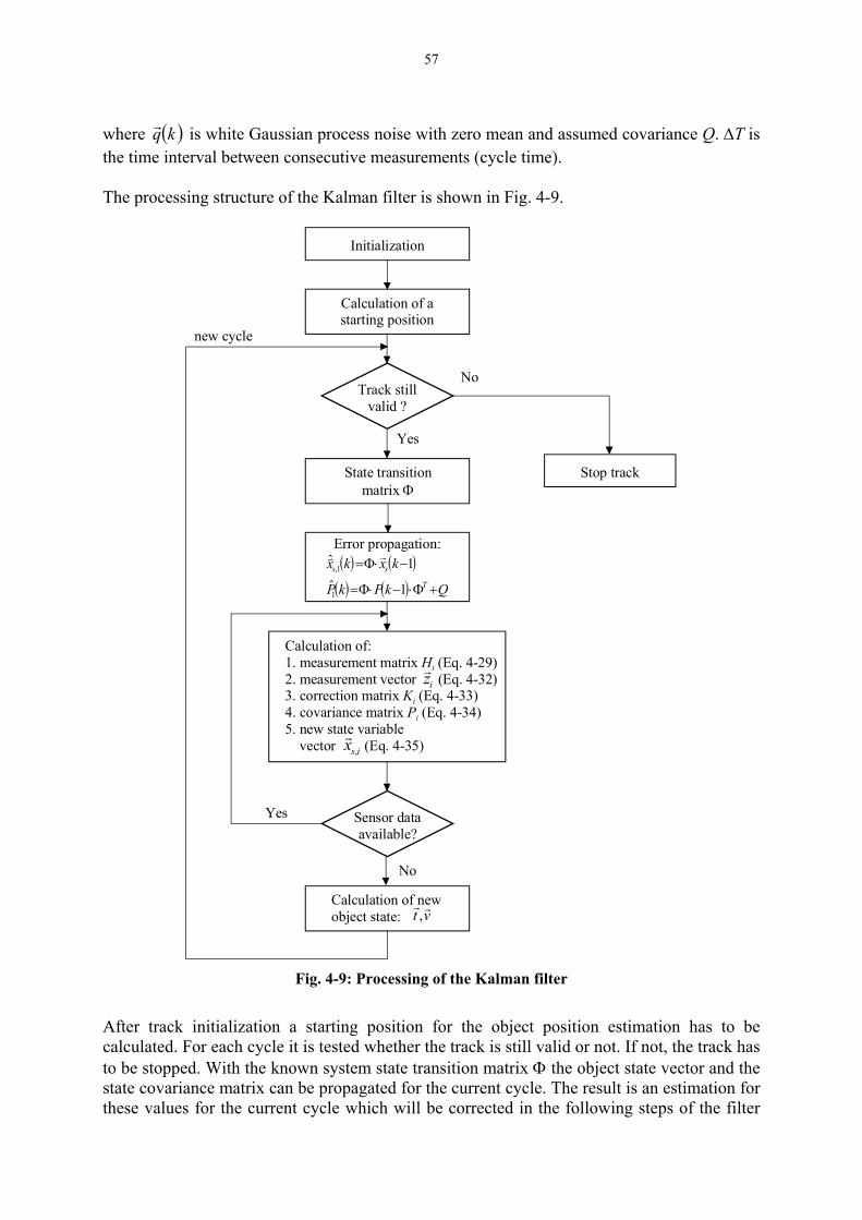
57

where is white Gaussian process noise with zero mean and assumed covariance Q. ∆T is the time interval between consecutive measurements (cycle time).

( )kqr

The processing structure of the Kalman filter is shown in Fig. 4-9.

Initialization

Calculation of astarting position

Track stillvalid ?

State transitionmatrix Φ

Error propagation:

Calculation of:1. measurement matrix Hi (Eq. 4-29)2. measurement vector (Eq. 4-32)3. correction matrix Ki (Eq. 4-33)4. covariance matrix Pi (Eq. 4-34)5. new state variable vector (Eq. 4-35)

Sensor dataavailable?

Yes

No

Yes

No

Stop track

Calculation of newobject state:

( ) ( )( ) ( ) QkPkP

kxkxT

ss

+Φ⋅−⋅Φ=

−⋅Φ=

1ˆ1ˆ

1

1,rv

new cycle

isx ,r

vt rr,

izr

Fig. 4-9: Processing of the Kalman filter

After track initialization a starting position for the object position estimation has to be calculated. For each cycle it is tested whether the track is still valid or not. If not, the track has to be stopped. With the known system state transition matrix Φ the object state vector and the state covariance matrix can be propagated for the current cycle. The result is an estimation for these values for the current cycle which will be corrected in the following steps of the filter

58

processing. Similar to an α - β - filter the Kalman filter also includes a prediction and an update step. The equations for error propagation in order to estimate the state vector and the state covariance matrix are for the first sensor (i = 1):

(4-26) ( ) ( )1ˆ1, −⋅Φ= kxkx ss

rr

(4-27) ( ) ( ) QkPkP T +Φ⋅−⋅Φ= 11̂

As indicated in Fig. 4-9 in the next step the measurement matrix for sensor i is calculated. The 2-dimensional measurement vector is modeled as:

( )kHi

( )kzir

(4-28) ( ) ( ) ( ) ( )knkxkHkz isiirrr

+⋅=

where is the measurement matrix of dimension 2x4 and vector is a model of the assumed zero-mean white Gaussian measurement noise with covariance R. It is assumed that all sensors have the same measurement noise characteristics R.

( )kHi ( )knir

The measurement matrix for the current cycle k and sensor i is calculated as follows based on object data from cycle k-1:

( )kHi

( )

( )( )

( )( )

( ) ( ) ( )( )

( )

( ) ( ) ( )( )

( )

−

−−−

⋅−−−

−

−−−

⋅−−−

−−−

−−−

=

001

1111

11

111

001

11

1

,

,,

,

,,

,,

kdkd

ykykvkv

kdkd

xkxkvkv

kdyky

kdxkx

kH

io

io

sitisy

io

io

sitisx

io

sit

io

sit

i rr

(4-29) where the direct distance between the specific sensor i and the estimated object position is denoted as:

( ) ( )( ) ( )( )22, 111 sitsitio ykyxkxkd −−+−−=− (4-30)

( )1, −kv is

r is the projection of the object velocity vector on the direct vector between the sensor i under consideration and the estimated object location. It is calculated by:

( ) ( ) ( )( ) ( ) ( )

( )111

1111

,,, −

−−⋅−+

−−−

⋅−=−kd

ykykvkd

xkxkvkvio

sity

io

sitxis

r (4-31)

The measurement of target distances are used to form the measurement vector . Due to the fact that the errors are estimated in this specific case, the vector is:

( )kzir

59

( )( ) ( )

( ) ( ) ( )

∆−−

−−

−−=

Tkrkrkv

krkdkz ii

is

iio

i 11

1

,

,

rr (4-32)

( )kri is the measured range to the detected target of sensor i (with i = 1...4) at time k.

With the results obtained above we can now get to a Kalman correction or gain matrix for the current cycle k and for sensor i, which is:

( )kKi

(4-33) ( ) ( ) ( ) ( ) ( ) ( )( 1ˆˆ −+⋅⋅⋅⋅= RkHkPkHkHkPkK T

iiiTiii )

The state covariance matrix update is then:

(4-34) ( ) ( ) ( )( ) ( ) ( ) ( )( ) ( ) ( )kKRkKkHkKIkPkHkKIkP Tii

Tiiiiii ⋅⋅+⋅−⋅⋅⋅−= ˆ

Having the Kalman correction or gain matrix we are now also able to update the a posteriori estimation for the state variable vector which is:

( )kKi

( ) ( ) ( ) ( ) ( ) ( )( )kxkHkzkKkxkx isiiiisis ,,,ˆˆ rrrr

⋅−⋅+= (4-35)

As shown in Fig. 4-9 the steps from measurement matrix calculation to state vector estimation update is done in a loop for each single sensor. The updated state vector is chosen as the estimated state vector for the next sensor in the loop: ( ) ( )kxkx isis 1,,

ˆ−=

rr

Finally the estimated object location and velocity information can be obtained for the current cycle using the last estimated a posteriori state variable vector : ( )kx is,

r

(4-36) ( ) ( ) ( )( ) ( ) ( )kvkvkv

ktktkt

err

errrrr

rrr

−−=−−=

11

with: and v (4-37) ( )

=

err

errerr y

xkt

r ( )

=

erry

errxerr v

vk

,

,r

For the next cycle the algorithm restarts with the error propagation of equations (4-26) and (4-27). Simulation showed that the algorithm can be a useful alternative to a least squares position solution and a following filter to increase system performance although the selection of parameters is more difficult. The combination of an object position solution and the optimal

60

tracking filter makes this algorithm a compact solution and especially suitable for cases where only a single sensor reports target detections. For the situation already described in chapter 4.3.2 the Kalman filter algorithm was simulated with the four sensor positions to and the following settings for the noise matrices Q, R and P:

2sr 5sr

=

005.00000005.00000001.00000001.0

Q

=

50003.0

R

=

100000100000100001

P

The cycle time ∆T was set to 20 ms and all sensor ranges were added with normally distributed noise of variance 3 cm. Fig. 4-10 shows the error of the object radius and angle estimated by the least squares algorithm and by the Kalman filter. The Kalman filter curve is the smooth curve in the diagram. The errors of the Kalman filter results are obviously smaller in both cases due to the smoothing properties of the filter. Fig. 4-11 shows the estimated Cartesian velocity components of the Kalman filter output.

-15 -10 -5 0 5 10 15-0.1

-0.08

-0.06

-0.04

-0.02

0

0.02

0.04

0.06

0.08

0.1

Distance from center line [m]

Erro

r of c

alcu

late

d ob

ject

radi

us [m

]

Error of object radius: calculated value - true value

-15 -10 -5 0 5 10 15-20

-15

-10

-5

0

5

10

15

20

Distance from center line [m]

Erro

r of a

zim

uth

angl

e [°

]

Error of azimuth angle: calculated value - true value (four sensors)

Fig. 4-10: Object radius error and angle error for Kalman filter and least squares solution

-15 -10 -5 0 5 10 15-1

-0.8

-0.6

-0.4

-0.2

0

0.2

0.4

0.6

0.8

1

Distance from center line [m]

Object velocity in x-direction

Obj

ect v

eloc

ity (x

-dire

ctio

n) [m

/s]

-15 -10 -5 0 5 10 150

0.2

0.4

0.6

0.8

1

1.2

1.4

1.6

1.8

2

Distance from center line [m]

Object velocity in y-direction

Obj

ect v

eloc

ity (y

-dire

ctio

n) [m

/s]

Fig. 4-11: Object velocity in x – and y – direction (Kalman filter)

61

The filter algorithm showed good results even when only a single range measurement was available. Normally a position solution with a single range could not be calculated, but the filter still tracks an object with only a single range measurement at the input.

4.4 Overview of a Multiple Object Multilateration and Tracking System An abstract model of a data fusion algorithm is depicted in Fig. 4-12. It shows the main steps from input of observations (measurements) to output of tracker results to a man-machine interface or a following application processor. Usually it is assumed that measurements may result from very different kinds of sensors. It is not necessary that all sensors are the same. Input sources may e.g. be also a long range radar, a video camera including image processing or an infrared laser. Data association of input data (e.g. to already existing tracks) is the first processing step. As indicated in Fig. 4-12 it is very useful to feed back information from the information database to the data association stage for association decisions, because decisions are much safer if supported by already known information. The situation database includes information and results of the previous processing cycle. This can be e.g. a set of object track state vectors or information about the own vehicle (e.g. own vehicle speed measured by ABS wheel sensors and accelerations measured by a gyro). It is also possible that results from the situation abstraction and assessment step are included. The data fusion can be started in the following step with all associations. For data fusion usually kinematic state estimation techniques like least squares algorithms or Kalman filter algorithms are applied. Results of the data fusion are the object state vectors saved in the situation database. A situation abstraction can be seen as an interpretation of all data of the information database not only from the current cycle, but also from all previous cycles. Results of the interpretation can be recognition of a driving mode or situation (e.g. parking aid, stop&go situation or a cut-in situation from a vehicle of an adjacent lane). Methods known from artificial intelligence can be applied for situation assessment. These can be e.g. expert systems, neural networks probably combined with fuzzy decision support or fuzzy decision algorithms alone.

Data Association

Data Fusion

Situation Database

Observations / Measurements

Situation Abstraction

Tracker Output Fig. 4-12: Abstract Data Fusion Model

Starting with the abstract data fusion model in mind, this chapter proposes different methods for a data fusion in an automotive radar network. Properties of the used sensors are taken under consideration for a decision in favour of a suited processing method.

62

In a first processing method with all detected sensor targets all possible intersections can be calculated. For one sensor the object position is assumed on a circle with the radius being the measured range to a detected target. With three or four ranges an iterative least squares algorithm can be applied to find an estimated position solution. From the obtained complete set of possible intersections all unlikely intersections can be deleted by a search algorithm. The set of intersections does not only include representations of real objects, but also false objects which have to be deleted for the following tracking. To find out false intersections, it is very useful to consider the situation database of preceding cycles. Deletion of false intersections without feedback of the situation database is not safe enough. In an implementation of this algorithm a large number of false intersections was observed. To find out correct intersections is very difficult and various false alarms occurred with real measured sensor data. An additional disadvantage is the large number of intersections which have to be calculated. Fig. 4-13 shows on the left side an implemented processing with included tracking of single sensor targets. After association of detected targets to single sensor target tracks the single sensor targets are tracked by means of an α - β - tracker. All sensor target tracks from different sensors are then associated to each other to find possible intersections for the object tracker. With all associations the possible intersections are calculated and fed into the object tracker. Intersections for three or four associated target tracks can be found by least squares iteration. It is assumed that a target is only originated by one object. That means that one single sensor target track can only be associated with one intersection. Multiple associations are excluded. Sensor target to target track associations from a previous cycle can be repeated, because the object was already validated before. This reduces the target lists of all sensors to the set of targets that possibly belong to a new object. These remaining target tracks can be associated to form new intersections for new objects. For all association steps the feedback of the object map and the intersection list is absolutely necessary to find correct decisions and to reduce effort.

63

Tracking ofSingle Sensor Data

Association of Targetsto Single Sensor Tracks

Association of Single SensorTracks for Intersections

Calculation ofIntersections

Tracking of Intersections(Objects)

Observations / Targets

Tracking ofSingle Sensor Data

Association of Targetsto Single Sensor Tracks

Association of Single SensorTracks for Intersections

Observations / Targets

Kalman - Filtering forCalculation of PositionSolution and Tracking

Feed Back of

Object-Map / Intersection ListFeed Back of

Object-Map / Intersection List

Fig. 4-13: Generalised Processing Overviews (α - β - Tracker and Kalman Filter)

A tracking of single sensor targets shows the following advantages and disadvantages:

• Advantages: + Short gaps of detection of a sensor are bridged by the target tracker. The number

of available sensor target tracks for a calculation of a position solution (intersection) is higher. This increases accuracy of an angle estimation.

+ A radial velocity can be estimated for each sensor track individually from range rates.

+ Many false targets can be filtered out, e.g. in situations where two sensors show interferences.

+ A pre-filtering of the target list reduces the amount of data to be processed. Disadvantages: • − Detected targets are passed after a few cycles to the following processing as

confirmed sensor target tracks. Results at the system output are delayed. A sensor target tracking shows important advantages and is seen as a required processing step in the radar network data fusion. For applications that require very low reaction times, the decision criteria for the tracker have to be optimised to achieve a low false alarm rate at low system reaction time. The sensor target association to target tracks is a step with important influence on the complete system performance. False objects in the object map may result by false target data association and the accuracy of measurements can be significantly reduced. A data association of detected targets to target tracks with consideration of the complete

64

situation showed to be very useful, because consecutive measurements are not independent from each other. In Fig. 4-13 on the left side the multilateration is divided into the estimation of a current position solution by means of a non-linear least squares estimation (chapter 4.3.1) and a following tracking. Both steps can be combined if a Kalman filter for the multilateration and tracking is used (chapter 4.3.4). The first steps remain unchanged compared with the processing structure shown in the left figure. Single sensor data association is nevertheless a very important step as well as association of sensor tracks to sets of up to four tracks each for the Kalman filtering. A calculation of an object position solution by multilateration and object state variable filtering is both integrated in the filter as already described in chapter 4.3.4.

4.5 Data Association Methods Data association is always a very crucial point in tracking and data fusion of radar systems and other multiple sensor systems. Wrong association may cause false objects or incorrect object coordinates at the tracking output. For angular accuracy and resolution in the multilateration radar network, data association is the key topic with highest importance. Association tasks can e.g. be a target to track association or a track to track association. The next chapters describe common association methods and how they can be applied to the considered network. A realistic example of a target to track association is shown in Fig. 4-14. Two sensor target tracks are already established and four new observations are detected and have to be associated. The question is now which observation can be associated to which track and which observation will be selected to start a new track that will be busy, but not yet active for further processing unless additional measurements confirm the track. It can be seen that observation C can be associated with both tracks because the gating intervals overlap. It is clear that only one track can be updated with this new observation. Multiple associations are usually excluded.

Sensor

Track 1

Gate 1Track 2

Observations

Gate 2

A

BC

D

Fig. 4-14: Target to track data association

The gating interval has only one dimension in the example shown above, but can usually be of different shape (e.g. rectangular or ellipsoidal). For one-dimensional or rectangular gating the relationship can be as follows ([BLA99]):

65

rCyy σ⋅≤− ~ with: 22por σσσ += (4-38)

tionnt/Observa Measureme:ytcoefficien Gating :C

position target Predicted:~y

deviation standard Residual :rσ t varianceMeasuremen :2

oσ variancePrediction :2pσ

The gating coefficient can be adjusted to the specific application. The measurement variance can be found e.g. by long term measurements of a target position whereas the prediction variance can be taken from the Kalman filter covariance matrix if a Kalman filter is applied.

4.5.1 Nearest Neighbor Association Methods Nearest neighbor methods only find a single most likely hypothesis in contrast to more sophisticated multiple hypotheses methods. To associate the nearest observation to the predicted target position of a track is nevertheless the most common technique and widely applied. Nearest does not necessarily mean the smallest geometrical distance, but can also be a statistical distance. From Fig. 4-14 it can be seen that association conflicts might occur when more than one observation is in one track gate or an observation is in more than one overlapping track gates. In this case an assignment matrix helps to get an overview of possible associations. The elements of the assignment matrix are cost values for the possible association. An example of an assignment matrix for Fig. 4-14 can be Table 4-1.

Observ. A Observ. B Observ. C Observ. D Track 1 d1,A d1,B d1,C 0 Track 2 0 0 d2,C d2,D

Table 4-1: Example of an assignment matrix

Some combinations are excluded for observations outside the gate. Fields for possible associations between track i and observation or measurement j are filled with the calculated statistical or geometrical distance. It is now of importance how to select the cost values within the assignment matrix. One solution can be the difference of the gate and a weighted norm (see also [BLA99], [BLA86]). The cost value is now a margin by which the statistical distance passed the gate G : 2

, jid ji,

(4-39) ( ) ( yySyyGdGa Tjijijiji

~~ 1,

2,,, −−−=−= − )

The matrix S is called innovation matrix and results from the Kalman equations (see also chapter 4.3.4):

(4-40) RHPHS T +⋅⋅= ˆ

66

4.5.2 Joint Probabilistic Data Association (JPDA) Nearest neighbor association methods only consider a single hypothesis for a measurement to track association. For a track with multiple measurements within the association gate, there are also other techniques known for an all-neighbors association approach. PDA (for probabilistic data association see [BLA86], [BLA99] or [BAR88]) forms multiple hypotheses after a single scan and combines all hypotheses weighted with calculated probabilities. All neighbors within the gate are considered, but measurements with higher probability are weighted more than measurements obviously caused by clutter. With this strategy all measurements contribute to the tracking update. For concrete information how to calculate the probability of a hypothesis, several publications can be found. The PDA method only assumes a single target while the JPDA method is an extension in order to handle multiple tracks and multiple measurements. To the high resolution radar network a probabilistic data association was not applied so far, but can be a technique to improve nearest neighbor method performance with limited additional expense.

4.5.3 Multiple Hypothesis Tracking (MHT) The main idea of MHT (multiple hypothesis tracking) is to form tracking hypotheses for all possible assignments and to propagate these hypotheses in order to resolve uncertainties in a later step of the processing with subsequent data. The advantage compared with simple gating and nearest neighbour association or JPDA is that a hard decision for the assignment is not performed until additional information is evaluated. Different hypotheses are tracked as different possible assignments. JPDA updates the track in the same cycle with a probabilistically weighted composite of all measurements observed within the track gate. The amount of data and complexity is limited with JPDA whereas in an MHT approach much information has to be tracked and processed from scan to scan. It is necessary to restrict a combinatorial explosion when using MHT. Possible techniques are e.g. clustering, hypothesis and track pruning or a track merging. These techniques are absolutely necessary to make the algorithm feasible for practical applications with high update rates as required in automotive radar systems. An implementation of an MHT algorithm can be accomplished as proposed by [REI79] and [BLA99]. The measurement-oriented approach and the track-oriented approach will be explained below and a short comparison reveals important features of both. An offline processed application of MHT on an automotive radar network can be found in [HAA00].

4.5.3.1 Measurement - oriented MHT An implementation of the measurement - oriented approach of MHT was first described by [REI79]. The proposed algorithm includes important features like multiple-scan correlation, clustering and recursiveness. Multiple-scan correlation allows a resolution of uncertainties by using subsequent as well as previous data. To divide the set of measurements and tracks into separate and independent groups is denoted by clustering. This allows the processing of independent groups of data. The complete problem can be divided into smaller subsets to make the processing faster and easier. Recursiveness can be accomplished by just using the

67

results of the previous scan and new measurements for a track update. Data from the preceding scan already includes all information from previous scans.

Receive new data set

Perform track update(Kalman-Filter)

Form new clusters:associate tracks and

measurements to clusters

Form new set of hypotheses:calculation of hypotheses

probability and track measurementupdate for each hypothesis of

all clusters

Simplify hypotheses matrixof each cluster; confirm tracks;

create new clusters forconfirmed tracks

Reduce number of hypotheses:elimination or combination

return for next scan

Fig. 4-15: Measurement-oriented MHT algorithm

The algorithm described by [REI79] starts with a set of new measurements obtained by the sensor(s) (see Fig. 4-15). A track update for the current cycle is the next step. Usually this is the extrapolation of the target state variables with the Kalman filter equations: with Matrix Φ being the state transition matrix ( ) ( )1ˆ −⋅Φ= kxkx ss

rr

In the following step recent measurements and tracks are associated with clusters and new clusters are formed for remaining measurements not associated with any existing cluster. As already explained, a cluster is a separation of the entire set of tracked targets into subsets which can be processed independently. For clusters being very close to each other, the individual clusters can be combined to a super-cluster. This may be the case for crossing tracks or extended objects like a vehicle with numerous backscatterers being very close to each other. If possible at this time a reduction of previously found hypotheses will already be carried out. Different possibilities to restrict the total amount of hypotheses are known from the literature. Very suitable techniques are e.g. an elimination of very unlikely hypotheses or a combination of very similar hypotheses. This reduction procedure is also used by the next processing stage which forms a new set of hypotheses from new measurements and the tracked targets. To form new hypotheses for a new set of measurements the typical measurement-oriented behaviour of the algorithm can be recognized. Starting with the first measurement, all

68

possible associations with existing target tracks in the cluster under consideration are listed. Then the next measurements are examined until the set of all possible hypotheses for all clusters is finished. For all hypotheses a probability can be calculated. [REI79] gives analytical results for the probability of a measurement to track assignment in the hypothesis matrix. Based on the probabilities very unlikely hypotheses can be neglected again by simple elimination (or pruning) or by combination of hypotheses. For all remaining hypotheses the track update is calculated using standard Kalman filtering algorithms. It is worth to reduce before updating the target track state variables, because the computational effort for complex Kalman filter equations can be kept as low as possible. To determine a new hypothesis, different requirements to be explained now have to be fulfilled. The measurement under consideration has to be within a specified validation gate around the track, e.g.:

( ) ( ) 21 ~~ η≤−− − yySyy T (4-41)

with: HS = and RHP T +⋅⋅ ˆ Hxy =~

Furthermore each track should not be associated with more than one measurement in the data set. Thus ambiguous hypotheses with lower probability have to be eliminated. After calculation of all possible and probable hypotheses and update of all tracks, the hypothesis matrix is simplified. Tentative tracks can be set to confirmed tracks and will be eliminated from the hypothesis matrix. With all tracks updated, the processing of a single cycle is finished and can be restarted with a new data set.

4.5.3.2 Track - oriented MHT An implementation of a track-oriented approach of MHT is described in [BLA99] and compared with a measurement-oriented implementation. Track-oriented means that for each single track the possible measurements are associated when forming hypotheses. This chapter describes the main processing steps of a track-oriented implementation. A track-oriented implementation is seen as having an advantage over the conventional measurement-oriented implementation proposed by [REI79]. One main advantage is seen in the reduced number of hypotheses due to the fact that low probability tracks are immediately deleted and only high probability tracks are maintained for further processing steps. The basic algorithm structure as explained in [BLA99] is shown in Fig. 4-16. The processing starts by forming and updating tracks for all measurements. All measurements are checked for possible associations with already existing tracks. This can be established by standard gating techniques. For possible assignments all combinations are kept disregarding possible multiple associations of measurements to more than one track. Usually it is assumed that a measurement can only be caused by a single object. Multiple associations are resolved later in the processing. Tracks without any new measurements within their gating region are only extrapolated. Measurements not associated to any track are recognized as a starting point of a new track. It is clear that many tracks will be formed and thus pruning techniques are

69

required to restrict the total number of tracks. Therefore the next processing step compares the calculated probabilities for each track with a fixed threshold and deletes all low probability tracks. Tracks sharing common measurements are defined to be incompatible and clustered in the next step. A cluster includes all tracks sharing common measurements, not only directly, but also if two tracks share measurements with a third track. The result of clustering is a list of interacting tracks ranked in order of likelihood.

Track Formationand Maintenance

Track Level PruningConfirmation

Clustering

Hypothesis Formationand Pruning

Global LevelTrack Pruning

Track Updatingand Merging

Tracks

SurvivingTracks

Measurements

TrackingOutput

Deletion Messages

Fig. 4-16: Track-oriented MHT algorithm

After clustering the formation of hypotheses starts. Each hypothesis consists of a set of compatible tracks, i.e. a set of tracks that do not share common measurements. The number of tracks within a hypothesis is not limited. For track pruning it is important to find the most likely hypotheses, i.e. the most likely set of tracks. This can be established by a search routine. If the most likely hypotheses are found, those of low probability can be deleted. The result is a list of hypotheses with each hypothesis consisting of a set of tracks. In the global level track pruning the tracks included only in deleted hypotheses can be deleted. Tracks with very low probability below a deletion threshold can be deleted, too. If the sum of probabilities of hypotheses including a track is calculated, this is also a probability of a given track. For all remaining tracks which should not be too many, the track updating can be calculated using standard Kalman filtering techniques. If track merging of parallel tracks with very similar state variable contents is possible, the tracks can be merged. All remaining updated tracks can now be output to following applications as a result of the MHT algorithm.

4.5.3.3 Comparison between both MHT Implementations For implementation in an automotive radar network the two possible implementations of the measurement-oriented approach and the track-oriented approach make sense. The following short comparison tries to identify which of both implementations is best suited for this application. The measurement-oriented approach maintains hypotheses from scan to scan and forms a hypotheses tree after more than one scan. A very large number of hypotheses may result and the tree has to be pruned. The algorithm proposed by [REI79] may result in tracking many hypotheses of low probabilities. The requirements on memory and computation power for a system having 10-20 ms cycle time can be quite high. In a track-oriented implementation, hypotheses are formed and reformed within the algorithm. Hypotheses are not maintained from scan to scan. This reduces the required memory space. The number of tracks maintained from scan to scan is also not too high, because tracks of low

70

probability are deleted. As a result the track-oriented approach seems to be more efficient for real-time applications with limited computer performance.

4.6 Description of an Implemented Radar Network Processing As shown in Fig. 4-17 in this network of four high resolution pulse radar sensors the individual target lists of all sensors are the multiple target tracker input. The system input is a set of Mk measurements at time k for sensors s:

( ) ( ){ 4...1;,...,2,1 , === sMmkZkZ kms } (4-42)

The maximum number of observations Mk from each sensor is set to ten observations per scan (20 ms) to limit the data to be transferred and to ensure that the processing time for all data is below the fixed cycle time. The required system output for following applications is a set of objects listed in an object map. Each object is described by its position relative to the car and its velocity components. The system output at time k is defined as:

( ) ( ){ } objects ofnumber maximum :with ,...,2,1 ooi nnikOkO == (4-43)

The first processing step with the sensor target lists is a single sensor target data association for the following single sensor target tracking. This observation to track association can use information of preceding cycles. To consider the previously calculated situation showed very good results for the data association. One advantage of using a separated single sensor target tracking is that the input to the following multilateration procedures is more continuous than without a single sensor target tracking stage. If omitted, it was observed that results were not satisfying enough with sensors of reduced sensitivity. The input for the single sensor target tracker has to be selected very accurate to achieve good results in the multilateration. Additionally the number of false targets that are passed to following processing stages with higher computation complexity is reduced. This is of advantage if sensor interference is observed or an increased number of false alarms due to clutter. How the sensor target to target track association is performed will be described below. The single sensor target tracking makes usage of an α - β - filter to update the estimation for target range and range rate of this sensor target track. After the single sensor target tracking stage all confirmed target tracks are passed to the multilateration procedures. The multilateration includes target track to track association techniques to find combinations of sensor target tracks that belong to objects. For all existing objects the sensor target tracks of the preceding cycle are used again. It is assumed that the target track is still caused by the same object and not by another object. These sensor target tracks can be identified by a target track identifier which is carried with the target track and which is also stored in the object data structure. With this processing all target tracks for existing objects can be associated again and removed from the set of target tracks to be associated with other target tracks. It is important to notice that the algorithm assumes that an object only causes not more than a single target track. All remaining target tracks have to be associated to each other to form new detected objects. This is accomplished by an elaborated search algorithm that checks possible

71

combinations first of two tracks and associates a third or even a fourth track if possible. Nearest neighbor gating criteria are used for the data association. This showed to be the fastest way which still produces good results. From all associated sensor tracks a list of intersections can be calculated. The solution is an intersection of two circle arcs for only two target tracks contributing to one object. For three or four target tracks a least squares algorithm is applied to find an optimal solution. This results in a list of intersections calculated from all combinations of sensor target tracks. This set of intersections gives a representation of the situation only for the current cycle. A subsequent tracking initiates object tracks from validated intersections observed within a few cycles. This requires an intersection to object track data association performed in each cycle to update the object track, initiate new object tracks and delete old and not updated object tracks. For this tracker a two-dimensional α - β - filter is applied to estimate the object position relative to the vehicle and also the Cartesian object velocity components. The result of the object tracking is the object map which is the output to the following application processor, e.g. a parking aid or stop & go algorithm that searches the list for a relevant object to activate the vehicle brakes or to accelerate if the street in front of the car is empty and the found objects are located on adjacent lanes. It was already mentioned that for sensor target to target track association information of the preceding cycle is used. This is the list of intersections and the object map. Each object carries the information of the contributing intersection with it as well as the identifier of the contributing sensor target tracks. From the identifiers the position of the target track in the list of sensor target tracks has to be found. With the found sensor target tracks a prediction of the intersection to the current cycle can be calculated using the estimated target track range rate. The predicted sensor target track ranges are in this case used for calculation of an intersection (using the least squares algorithm) which is denoted as the predicted intersection. From this predicted intersection the expected ranges for the sensor targets detected in this current cycle can be determined. With these expected target ranges the target to sensor target track association is performed using a gate depending on the vehicle speed and nearest neighbor data association techniques.

72

Read Target Lists

Find Track Positions

List of TrackedObjects

List of TrackedSensor Targets

Calculate predicted intersections Target to Sensor TargetTrack Association

Single SensorTarget Tracking

Association of Tracked Targetsto existing Object Tracks

Multilateration:Calculation of new Intersections

Association of Intersectionsto Object Tracks

Object Tracking

Output of Object Map

TrackedTarget Lists

List ofIntersections

List of TrackedObjects

Associations between Targetsand Sensor Target Tracks

Associations betweenIntersections and Object Tracks

Indices of used Tracks

Distances between predictedIntersections and Sensors

Fig. 4-17: Radar network processing overview

The main advantage of the described processing with a feedback of information from the previous cycle is that the sensor target tracking is not performed independent from each other from sensor to sensor. A prediction for the intersection is used in the current cycle. This includes contributions for the position estimation from all four sensors. Therefore it is not possible that one sensor target track range can drift away from the other sensor target track ranges caused by wrong sensor target to track data association. So for each sensor track the detected target will be associated that fits best to the complete predicted object position. This processing showed very good results with simulated and also real data. For the existing software a separation of position estimation using least squares algorithms and track filtering was selected to have a better overview of the system intermediate results with this blockwise processing. In the case of application of a Kalman filter the optimal position estimation and the filtering would be one single block in the complete processing (see Fig. 4-13 (right side)). Intersections representing an instantaneous unfiltered object position without respecting the object position history would not be calculated in this case.

73

5 Phase Monopulse Sensor Concept With the conventional sensor concept (Fig. 3-2) and the use of e.g. four sensors distributed in a bumper with distances up to 50 cm between each other, all sensors receive reflections from different backscatterers of a complex target like a vehicle. Angle estimation by means of sensor to sensor data association of target list data and multilateration is a difficult task in this case. Improvements can be achieved by providing more information about single detected targets to the data association algorithm. A rough estimation of object angles by each single sensor and a more precise estimation in a central processor by using data of three or four sensors would be an interesting concept on the way to avoid false objects caused by a wrong data association. The idea of estimating a target angle already in the single sensor processing stage can be realized by a new concept proposed in this chapter. Important system parameters are discussed to evaluate the performance improvement compared with already existing systems.

5.1 Concept Overview On the basis of the conventional concept, Fig. 5-1 depicts the modified radar frontend. The idea is to use two rather than only one receive path in the sensor while the complete transmit path remains unchanged. For transmission a patch array antenna on one side of the sensor is used and for signal reception two separated receive antenna patch arrays on the other side of the sensor frontend are located with distance dx1 and dx2 to the transmit antenna. The distance ∆dx = dx2 – dx1 between both receive antennas in a single sensor has to be less than the carrier frequency wavelength λ in order to avoid ambiguities for the estimated angle. The distance to the transmit antenna is a trade-off between low signal crosstalk from the transmit to the receive antenna and sensor size. It is assumed that reflected pulses reach the receive antennas in a parallel wavefront. In this case the object angle α can be calculated as (see Fig. 5-3):

∆⋅∆⋅

=dxπϕλα

2arcsin (5-1)

with a phase difference of between both receive signals and under the assumption that with ∆dx smaller than λ no ambiguities can occur. For small errors of the signal phase difference the resulting object angle error is proportional to the signal phase error. For a distance λ between the receive antennas the resulting object angle error is approximately one degree for six degrees of phase difference error. The angle estimation accuracy can be improved with exclusion of ambiguities if a maximum detection angle of e.g. 45 degrees is assumed for the sensor. For this case the distance between both receive antennas can be

21 ϕϕϕ −=∆

λ⋅= 2dx∆ . For an error of 8.9 degrees for the signal phase difference the object error will be one degree (see Fig. 5-2). Angle estimation can still be better than the result of a single sensor if a least squares estimation of the object position in the complete network of up to four sensors is considered.

74

ReceiveAntenna 2

TransmitAntenna

dx1

ReceiveAntenna 1

dx2 Fig. 5-1: Frontend of the phase

monopulse sensor

-20 0 20 40 60Signal Phase Error [°]

gle Error vs. Signal Phase Error (dx=1.4*lambda)

Obj

ect P

ositi

on A

ngle

Erro

r [°]

Object An

-60 -40

-8

-6

-4

-2

0

2

4

6

8

Fig. 5-2: Object angle error vs. phase error

Transmit

Receive

α∆dx

Fig. 5-3: Wavefront reconstruction with a phase monopulse concept

Fig. 5-4 shows the sensor RF frontend hardware structure in detail. Triggered by the PRF generator, the 24 GHz DRO pulses are transmitted as before. Both symmetrical receive paths are triggered with an adjustable delay set by an external sweep control. Each receive path consists of an inphase and a quadrature channel, i.e. the delayed pulses from the DRO are in one case directly provided to the sampling phase detector and in the other case provided with a phase shift of 90 degrees for the quadrature channel. This is done in both receive paths. It should be emphasized that both receive paths are triggered with the same adjustable delay.

75

td

PRFGenerator

AdjustableDelay

24GHzDRO

PulseGenerator

PulseGenerator

3dB PowerSplitter

High SpeedSwitch

TransmitAntenna

LO/I

IF 1/IOutput

ReceiveAntenna 1

90°

IF 1/QOutput

LO/Q

RF/I

RF/Q

LO/I

IF 2/IOutput

ReceiveAntenna 2

90°

IF 2/QOutput

LO/Q

RF/I

RF/Q

SweepControl

PulseGenerator

High SpeedSwitch

High SpeedSwitch

High SpeedSwitch

Fig. 5-4: Block diagram of the sensor concept

To estimate a target angle it is important to be able to calculate a signal phase within each receive path by evaluation of the IQ-signals. The angle estimation can then be accomplished by phase comparison of both receive paths. Depending on the wavelength which is 1.24 cm with a 24.125 GHz DRO ambiguities may result for the estimated angle depending on the distance between the receive antenna patch arrays. If necessary, ambiguities have to be resolved in the central processor. Within the single sensor an angle estimation using the known multilateration concept or amplitude monopulse techniques would not be feasible due to the very small base length between the two receive antennas. It was already shown how the resulting object angle error depends on the signal phase errors (see Fig. 5-2). The required accuracy for phase measurement is different for the possible applications with different requirements concerning object angle measurement. An accuracy of one degree for the object angle means a maximum error of approximately 8.9 degrees for the phase difference which seems to be feasible. One main factor causing phase errors can be an unsatisfactory orthogonality of I- and Q-channel. In reality there is always an angle slightly different from 90° between both which can be calibrated (see [CHU81]).

76

For automotive applications the frequency band at 77 GHz as well as the ISM band at 24 GHz are considered for future systems. For the idea described in this chapter the ISM band is very suitable due to the higher wavelength (λ = 1.24 cm) compared with 77 GHz (λ = 3.9 mm). Ambiguities can be avoided. On the other hand a sensor at 24 GHz requires a bigger antenna aperture. The sensor concept might also allow an estimation of the signal distortion caused by crosstalk from the transmit to the receive antenna. Crosstalk is caused by propagation outside the sensor and inside depending on the RF layout and on the sensor design. The distortion can be reduced because real targets have the same amplitude in both receive paths while crosstalk influence is different in both paths due to different distances to the transmit antenna.

5.2 Data Fusion in the Phase Monopulse Sensor Network If a single sensor is only able to give a rough estimation of target angles it is an important question how the angle estimation can be improved in the complete system by using the redundancy when measuring with e.g. three or four sensors. To answer this question the Kalman filter modifications of the filter algorithm shown in chapter 4.3.4 will be explained and some simulations convince how the additional angle estimation within a single sensor improves the system performance. A data fusion overview shown in Fig. 5-5 includes the main elements of the data association and tracking software running on a central processor. The input vectors from all sensors (e.g. four) include range information as well as an estimated target angle. After target to track association, an individual tracker for all sensors tracks the targets and a following track to track association finds sensor track combinations of all objects to be tracked. The set of associated sensor tracks is the Kalman filter input. This extended Kalman filter (see also [BAR93]) is used to find a position solution of the object and tracks the object coordinates. From polar input coordinates of all four sensors with their individual aspect to the object, the tracker produces filtered Cartesian output coordinates of the tracked object.

r1,α1 r2,α2 r3,α3 r4,α4

Kalman Filter

(x,y,vx,vy)

Target to Track Association& Sensor Tracker

Track to Track Association

r1T,α1Τ r2T,α2Τ r3T,α3Τ r4T,α4Τ

(r1T,α1Τ/r2T,α2Τ/r3T,α3Τ/r4T,α4Τ)

Fig. 5-5: Data Fusion Overview

77

The filter equations are very similar to the filter described above in chapter 4.3.4 with the difference that an extension for measured angles is integrated and the derivation of the measurement matrix and the state transition matrix is accomplished by calculation of the Jacobian matrices. Furthermore not the position and velocity estimation errors are included in the state vector, but the object position and velocity themselves. It is important to mention here that the matrices should not be exchanged by mistake with the matrices in chapter 4.3.4. The notation is very similar for better comparison between both methods. For the sensor locations within the sensor network the following coordinates are used:

=

1

11

s

s

yx

sr (5-2)

=

2

22

s

s

yx

sr

=

3

33

s

s

yx

sr

=

4

44

s

s

yx

sr

The target ranges and angles are measured by each sensor individually at time k: with: i = 1…4 for four sensors ( ) ( )kkr ii α, The initial situation of the algorithm is an estimated object state vector of the previous cycle:

State estimate at time tk-1: (5-3) ( )

( )( )(( )

−−−−

=−

1111

1

,

,

kvkvkykx

kx

oy

ox

o

o

sr

)

)

A state prediction for the current cycle at time tk can be calculated in nonlinear systems with the general form represented by a function f:

(5-4) ( ) ( )( 1ˆ −= kxfkx ssrr

In the specific system modelled in this report the system equations are linear:

( ) ( )1ˆ1, −⋅= kxFkx ss

rr (5-5)

with the state transition matrix: and (5-6)

∆

∆

=

10000100

010001T

T

F ( )

( )( )( )( )

=

kvkvkykx

kx

oy

ox

o

o

s

,

,1,

ˆˆˆˆ

r̂

The derivation of the linear state transition and measurement matrices in this case are obtained by calculation of the Jacobian of a function. The general form of a Jacobian of a vector-valued function g using the gradient operator is:

( )xg x

x∇

78

( ) ( )[ ] ( ) ( )[ ]

∂∂

∂∂

∂∂

∂∂

=

∂∂

∂∂

=∇=∂∂

=

n

mm

n

T

m

n

TTxx

xg

xg

xg

xg

xgxg

x

xxg

xgxg

L

MOM

L

LM

1

1

1

1

1

1 (5-7)

The Jacobian of the state transition function is in our case the state transition matrix itself due to the linearity of the system equations. The state transition matrix is linear and time-invariant in this case:

( )( )

∆

∆

=∂

−∂=

−=

10000100

010001

11

TT

xkfF

kxx sr

(5-8)

The next step is to find a prediction for the measurements of sensor i. It is a function h of the state prediction for the current cycle k. The general form is:

( ) ( )( )kxhkz isi ,ˆˆ rr

= (5-9)

The predicted state vector has to be corrected at the end of the algorithm within each loop of a single sensor. A measurement residual between the real noise-added measurements and the predicted measurements for the current cycle and for sensor i is weighted with a filter gain or correction matrix W to compensate errors of the state prediction:

( )kx is,r̂

( ) ( ) ( ) ( ) ( )( )kzkzkWkxkx iiiisisˆˆ

,,rrrr

−⋅+= (5-10)

with the real sensor measurements added with noise : ( )kzi

r ( )kwr

(5-11) ( ) ( )( ) (kwkxhkzirrr

+= ) The vector with the real measurements is as follows: ( )kzi

r

( )( )

( ) ( )

( )

∆−−

=

kT

krkrkr

kz

i

ii

i

i

α

1r (5-12)

The three elements of the vector of sensor i are the measured range r, a range rate from the current cycle range and the previous cycle range, and the measured angle.

79

The vector of the estimated measurements is:

( )

( )( ) ( )( )( )( )

( )( ) ( )( )( ) ( )( )

( )( ) ( )( )( )

( )( )

−−

−⋅

−+−

−+−⋅

−+−

−

−+−

=

sio

sio

y

siosio

siox

siosio

sio

siosio

i

xkxyky

kvykyxkx

ykykvykyxkx

xkx

ykyxkx

kz

ˆˆ

arctan

1ˆˆ

ˆ1

ˆˆ

ˆ

ˆˆ

ˆ0,220,22

22

r

(5-13) The measurement residual for the system under consideration is: ( ) ( )kzkz iii

r̂rr−=ν

( ) ( )( ) ( )( )( ) ( ) ( )( )

( )( ) ( )( )( ) ( )( )

( )( ) ( )( )( )

( ) ( )( )

−−

−

−⋅

−+−

−+−⋅

−+−

−−

∆−−

−+−−

=

sio

sioi

y

siosio

siox

siosio

sioii

siosioi

i

xkxykyk

kvykyxkx

ykykvykyxkx

xkxT

krkr

ykyxkxkr

ˆˆ

arctan

1ˆˆ

ˆ1

ˆˆ

ˆ1

ˆˆ

0,220,22

22

α

νr

(5-14) The filter gain or correction matrix W for sensor i can be obtained by the following equations:

( )ki

State prediction covariance matrix at the beginning of a cycle:

( ) ( ) QFkPFkP T +⋅−⋅= 11̂ (5-15)

State prediction covariance matrix in the loop:

(5-16) ( ) ( ) QFkPFkP Tii +⋅⋅= −1

ˆ

with the system noise covariance matrix: Qand the Jacobian of the state transition function f: ( )1−kF

Residual covariance matrix: (5-17) ( ) ( ) ( ) ( ) RkHkPkHkS Tiiii +⋅⋅= ˆ

with the measurement noise covariance matrix: R and the Jacobian of the measurement function h: ( )kHi

Filter gain or correction matrix for sensor i: (5-18) ( ) ( ) ( ) ( )kSkHkPkW iTiii

1ˆ −⋅⋅=

80

Finally the predicted state covariance matrix has to be updated for the next sensor i+1 of the same cycle k or for the next cycle:

(5-19) ( ) ( ) ( ) ( ) ( )kWkSkWkPkP Tiiiii ⋅⋅−= ˆ

For the Jacobian of the measurement equations the following measurement matrix H for sensor i at time cycle k is obtained:

( ) ( )( )

( )( )

( )( )

( )( )

( )( )

( )( )

( )( )

( )( )

( )( )

( )( )

( )( )

( )( )

( )( )

( )( )( ) ( )( )

( )( )( ) ( )( )

( )( )( ) ( )( )

( )( )( ) ( )( )

( )( )( ) ( )( )

( )( )( ) ( )( )

−+−−

−+−−

−

−+−⋅∆

−

−+−⋅∆

−−+−

−

−+−

−

=

=

∂∂

∂∂

∂∂

∂∂

∂∂

∂∂

∂∂

∂∂

∂∂

∂∂

∂∂

∂∂

=∂

∂=

=

00ˆˆ

ˆˆˆ

ˆ

00ˆˆ

ˆ

ˆˆ

ˆ

00ˆˆ

ˆ

ˆˆ

ˆ

ˆˆ

ˆˆ

ˆˆ

ˆˆ

ˆˆ

ˆˆ

ˆˆ

ˆˆ

ˆˆ

ˆˆ

ˆˆ

ˆˆ

2222

2222

2222

0,,

0,,

0,,

ˆ

siosio

sio

siosio

sio

siosio

sio

siosio

sio

siosio

sio

siosio

sio

y

i

ox

i

o

i

o

i

y

i

ox

i

o

i

o

i

y

i

ox

i

o

i

o

i

kxxi

ykyxkxxx

ykyxkxyy

ykyxkxT

yy

ykyxkxT

xxykyxkx

yy

ykyxkx

xx

kvk

kvk

kyk

kxk

kvkv

kvkv

kykv

kxkv

kvkr

kvkr

kykr

kxkr

xkhkH

ααααr

(5-20)

The Kalman filter processing is performed as explained in Fig. 5-6. For each cycle a loop over all sensors is calculated to find an optimal and filtered position solution. At each new cycle the state and covariance matrix prediction has to be evaluated once (Eq. (5-21) and Eq. (5-22)) before running the loop over all sensors.

81

Initialisation

Calculation of astarting position

Track stillvalid ?

State transition matrix F

State / Covariance prediction:

Calculation of measurementJacobian matrix Hi(k)

Calculation of measurementresidual:

Calculation of residual covari-ance Si(k), and filter gain Wi(k):

Calculation of updated statecovariance matrix:

Calculation of new state variablevector:

Sensor dataavailable?

Yes

No

Yes

No

Stop track

Calculation of newobjekt position

( ) ( )( ) ( ) QFkPFkP

kxFkxT

ss

+⋅−⋅=

−⋅=

1ˆ1ˆ

1

1,rr

( ) ( ) ( )kzkzk iiir̂rr

−=ν

( ) ( ) ( ) ( ) ( )kWkSkWkPkP Tiiiii ⋅⋅−= ˆ

( ) ( ) ( ) ( ) ( )[ ]kzkzkWkxkx iiiisisˆˆ

,,rrrr

−⋅+=

( ) ( ) ( ) ( )( ) ( ) ( ) ( )kSkHkPkW

RkHkPkHkS

iTiii

Tiiii

1ˆ

ˆ−⋅⋅=

+⋅⋅=

Fig. 5-6: Extended Kalman Filter Processing

82

5.3 Data Fusion Simulation Even an angle estimation of low precision can improve the system performance significantly. Simulation results of the extended Kalman filter are shown in Fig. 5-7 and Fig. 5-8. The situation is an object at 15 m in front of the car moving from the left side (15 m) to the right side (-15 m). All sensor ranges are added with Gaussian noise of 3 cm variance. Object angles are all added with Gaussian noise of 2.86°. The sensor location settings are the same as sensors 2 to 5 in chapter 4.3.2. Between 12 and 20 seconds only sensor 1 was used for object tracking. From Fig. 5-7 (right side) it can be seen that the estimated object angle with only a single sensor detecting the object is still of good quality. The estimated velocity components (Fig. 5-8) are also nearly unchanged even with reduced input of sensor data. Simulation of the same situation with the filter described in chapter 4.3.4 showed growing errors with only a single sensor detecting the object. For two sensors detecting the object the obtained results are very similar.

0 5 10 15 20 25 30-0.1

-0.08

-0.06

-0.04

-0.02

0

0.02

0.04

0.06

0.08

0.1

Time [s]

Erro

r of c

alcu

late

d ra

dius

[m]

Error of calculated radius: calculated - true value

0 5 10 15 20 25 30-5

-4

-3

-2

-1

0

1

2

3

4

5

Time [s]

Erro

r of c

alcu

late

d az

imut

h an

gle

[°]

Error of calculated angle: calculated - true value

Fig. 5-7: Object radius error and angle error for extended Kalman filter

0 5 10 15 20 25 30-1

-0.8

-0.6

-0.4

-0.2

0

0.2

0.4

0.6

0.8

1

Time [s]

Vel

ocity

(x-d

irect

ion)

[m/s

]

Velocity (x-direction)

0 5 10 15 20 25 300

0.2

0.4

0.6

0.8

1

1.2

1.4

1.6

1.8

2

Time [s]

Vel

ocity

(y-d

irect

ion)

[m/s

]

Velocity (y-direction)

Fig. 5-8: Object velocity in x – and y – direction for extended Kalman filter

The following noise matrix settings were chosen for the simulation:

83

=

01.0000001.00000003.00000003.0

Q

=

05.0000500003.0

R

=

0.1000000.1000000.100000.1

P

(5-23)

5.4 Combination of Amplitude Monopulse and Phase Monopulse Techniques Application of phase monopulse techniques showed feasibility of angle estimation already in the single sensor stage. It is obvious that for the data association as well as for the multilateration and tracking results it is of advantage to get this additional angular information. When time synchronization between the sensors is also achieved, the target amplitudes of all sensors can be used in the central processor to get an additional angle estimation using conventional amplitude monopulse techniques. These methods can be applied after target to target association in the central processor.

5.5 Conclusive Discussion of a Phase Monopulse Sensor Network A short comparison of advantages and disadvantages concludes the description of the phase monopulse sensor concept. The two main advantages are that the angle tracking results with a single sensor detecting an object is much more precise than before and that data association of targets to sensor tracks is easier than before. With correct data association the number of false alarms should be significantly reduced. Advantages of the concept are:

1. Possibility to measure an object position angle with each single sensor and use this information as a contribution in the central processor to improve system performance and reliability.

2. The required very precise range measurement with the system described before is relieved because an additional angle information received by each sensor improves object angle estimation in the central processor if ranges are less accurate.

3. Angle estimation in each sensor is independent from non-linearities or temperature dependent variations of the adjustable delay for the receive paths. For the phase measurement only the difference of propagation time is of importance.

4. Situations with extended targets having multiple backscatterers or changing backscatterer positions in dynamic situations can be handled easier. The effort for data association algorithms within the software of a central processor can be significantly reduced.

5. Angular resolution can be accomplished by clustering of targets from the four sensors in the central processor and tracking of distinguishable clusters.

6. In situations when only a single sensor detects the target, tracking results are of very good quality compared with a sensor network that only measures target ranges.

Disadvantages of the concept are:

1. Increased cost for sensor RF frontend hardware due to the second receive path. 2. Larger antenna aperture with a second receive antenna patch array.

84

85

6 Experimental Short Range Radar Network Practical feasibility of a short range radar network was studied by means of an experimental vehicle. The following chapters give a brief system description.

6.1 System Description For experimental evaluation of theoretical aspects in a short range radar network, a normal passenger car was modified to be used for the safety and comfort applications described above. The purpose and importance of the vehicle covers multiple aspects. These are for example:

• Acquisition of realistic traffic data on normal roads and highways in very different situations. Realistic data files are an important data base for improvement of detection and sensor data fusion techniques in the laboratory.

• Real-time display capabilities are important to show the system performance and all vehicle data on a notebook in the car.

• In combination with the actual street situation recorded on video tape in parallel to radar data, the radar results can always be evaluated considering the video reference.

• Observing the very complex system’s real-time behavior in real traffic situations and as a target data source for an adaptive cruise control system with an electronic addressable brake and cruise controller.

• Observing the reflectivity and complexity of very different real objects with a diversity that can not be replicated in a normal laboratory (e.g. reflectivity of trees, metal fences, crash barriers, bicycles, passengers, traffic signs, bridges or even different road surface conditions).

• Experimental vehicle as a development platform to show feasibility of a system which will surely become a new feature in future vehicles.

• With the possibility to simply change the vehicle front bumper the performance of different sensors and sensor networks can be directly compared.

Without the possibility to have access to real data the development of such a system could disregard important practical aspects and conditions while some aspects which might be of theoretical importance show to be of minor interest in a real system. To stay as close to practical applications and feasibility as possible was always the intention during the whole development of this system. The implementation of a short range radar network based on four 24 GHz pulse radar sensors is shown in Fig. 6-1. The sensors are usually covered in this car and can be mounted behind a vehicle bumper to make the car look like any other car. A block diagram of the experimental vehicle equipment is presented in Fig. 6-2. The car is equipped with an addressable brake booster and a modified cruise controller for adaptive cruise control applications. A microcontroller (SAB 80C167) handles communication between the RDU and the cruise controller. It also measures the wheel rotation time of all four wheels. The interface to the RDU is the CAN bus the brake is also connected to. All sensors have a CAN interface to be connected directly to the RDU in a common bus or each of them separately. The RDU serves as sensor supply and as a central data fusion processor. The RDU functionality will be explained in the following chapter.

86

Fig. 6-1: Short range sensor network integrated in a vehicle front bumper

ABS

CruiseController

externalsignals

Notebook/VGA Display

Veh

icle

CA

N

Brake-Booster 80C167

RadarDecision

Unit

HRRDSP

HRRDSP

HRRDSP

HRRDSP

Ethe

rnet

/CA

N o

r VG

A

+12V

CA

N a

nd S

enso

r Sup

ply

Fig. 6-2: Experimental vehicle equipment

87

6.2 Radar Decision Unit Overview Processing of all radar data is accomplished in an industrial PC (Fig. 6-3 (left side)) mounted in the back of the vehicle. Input for this so-called radar decision unit are target lists from each individual pulse radar sensor. Output is the so-called object map which is a list of detected objects with distance, angle and speed. The sensors integrated in latest developments include integrated processing capabilities and distance self-calibration to achieve a distance measurement accuracy of less than ±3 cm over the complete range of up to 20 m. This precision was measured with the automatic self-calibration and test system described in chapter 7.1 and is the key sensor feature to achieve high performance with the system. The radar decision unit (Fig. 6-4) is a very flexible data fusion processor in the system. It covers the following tasks:

• Data acquisition of all sensor target lists from the high resolution radar sensors mounted in the subsystem under consideration (e.g. front or rear bumper). In this stage of showing feasibility, all sensors have an individual CAN bus to the RDU.

• Sensor target lists are received by a microcontroller which transfers all data to a fast dual ported RAM mounted as a daughter-module on a PCI DSP board (TMS320C6701 evaluation board). The microcontroller CAN board and the PCI DSP board with DPRAM daughter-module is depicted in Fig. 6-3 (right side).

• The task of the DSP is to combine all target lists to get a representation of the real street situation (object range, angle and speed). The DSP is timer-triggered with 20 ms cycle time and interrupts the microcontroller via DPRAM to start a new cycle of target data collection.

• The microcontroller has an additional own on-chip CAN interface to read vehicle data like own speed or the current curve radius and to control brake and cruise controller. Control algorithms are included in the data fusion processor (DSP) which calculates a required brake pressure or vehicle speed. This information is passed to the microcontroller’s CAN interface.

• For real-time visualization in the drivers cockpit the objects detected by the RDU are passed via PCI bus to an all-in-one PC board which is the main processing board booting the operating system from hard-disk on system start.

• The PC board in this case has all required interfaces on board, like a normal mainboard including an Ethernet interface. With its interfaces, the PC is able to record data files while driving, to display object map data or vehicle data in real-time using an external VGA display. A DirectX display running on the PC showed very fast update rates of a few milliseconds ([WEN00]). Transmission of all data via Ethernet e.g. by means of Client-Server sockets showed to be another very flexible possibility for an RDU display.

On system start all sensors boot up individually and unsynchronized to each other. The microcontroller starts from its Flash-Eprom and waits for DSP triggers to collect data. The PC boots automatically and starts a Windows-based application which loads an executable file to the DSP board, starts the DSP software and transmits all results to a display tool (if connected as a client application to the server). So the complete system is self-starting and shows much potential for modification of software and experiments in an early stage of system development and feasibility study as well as system performance tuning.

88

Fig. 6-3: RDU industrial PC with data acquisition CAN board and DSP hardware

Fig. 6-4: Radar Decision Unit Overview

The software running on the PC (see Fig. 6-5) includes features which appeared to be important for fast signal processing development with the experimental system. All measured system data can be saved on hard-disk. Individual sensor target lists can be saved during measurements and used in the laboratory to improve data fusion algorithms. Target list files can be loaded and the data fusion can be processed in a very convenient Windows-based development environment for debugging or on the DSP board to measure execution time of the data fusion software on the DSP. This can be used to estimate which maximum processor performance is required in a later serial system. To be able to debug the software in a very convenient environment and directly test data fusion software modifications with real data was a way of very fast progress for the complete system. It is furthermore possible to send large blocks of data from each sensor (up to 512 CAN messages per cycle of approximately 100 ms) to directly have a look at the analog sensor output signal which is sampled by an on-chip A/D-converter of the sensor DSP. With this feature raw sensor data can be recorded in dynamic street situations.

89

Fig. 6-5: Online display in the driver’s cockpit

6.3 Network Communication Considerations Communication of data in the sensor network is an important topic and different factors influence the selection of a bus system or protocol. The required data rate is not the only aspect. Especially for a radar sensor network in a vehicle, the following points have to be considered:

• Safe transmission of all data in an electromagnetic influenced environment • Serial communication with only a few wires to be integrated into the vehicle • Fast bus access of the individual sensors to a common bus interface • Availability of cheap communication controllers (as cheap stand-alone controllers or

as on-chip interface controllers on commercial microcontrollers) • Low amount of overhead for data transmission • Capability to send short messages with low effort and overhead • Extension of the network over a few meters without transmission errors • Flexible number of nodes in the network and correct communication if individual

nodes fail A very good overview of common transmission protocols and busses and evaluations for a vehicle sensor network is given in [KUH00]. The required data rate for a system of four sensors has to be evaluated to find out which communication platform is suitable for a vehicle sensor network. Each sensor transmits e.g. an amount of 10 targets per cycle with 8 Bytes per target message and a cycle time of 20 ms. The complete data rate for a bumper equipped with four sensors is:

90

skBit

D ms

12820ms

1Bit64104

Time Cycle1gthMessageLenNumTargetsNumSensorsTargets10,20,Sensors4

=⋅⋅⋅=

⋅⋅⋅= (6-1)

One target message includes distance information, amplitude, velocity (if measured) and a time stamp. If the realistic number of 10 targets per sensor and cycle in a range of up to 20 m is not sufficient, the data rate increases. Additionally the cycle time of 20 ms is too long for applications with high demand on security. A cycle time of 10 ms would be better. For these requirements a worst case estimation with 20 targets would be:

skBit

msBitD ms 512

10164204Targets20,10,Sensors4 =⋅⋅⋅= (6-2)

It should be noted that this data rate is only relevant data, but no header information. All header information has to be added to get the maximum bus load for the communication bus to be selected. In this thesis a maximum number of 10 targets, a maximum cycle time of 20 ms is assumed and a data rate of 128 kBit/s. For a first system all sensors were separated and connected to the RDU via individual CAN busses. One CAN bus is able to handle a maximum data rate of 1 Mbit/s including data and header. To guarantee safe transmission, a maximum bus load of 40% is a good compromise. For a CAN bus the header of a 64 Bit data message is 47 Bit (total = 111 Bit). The relevant data rate for one bus with a maximum bus load of 40% is then approximately 230 kBit/s. With the capacity of one CAN bus, data compression can be applied to manage four sensors on one CAN bus. The properties of CAN are very attractive to use it in a sensor network and the price of a CAN node is very low compared with other interfaces, because CAN is widely used today for many applications. If more capacity is needed different new interfaces are interesting. These are e.g. MOST (Media Oriented Systems Transport with up to 50 MBit/s), Byteflight (up to 10 MBit/s data rate) or TTP (Time-Triggered Protocol, a system with TDMA protocol).

6.4 Sensor Network Synchronization It was already explained that precision in range measurement of approximately 3 cm is desired to achieve good results for angle estimation. With a cycle time of 20 ms Table 6-1 shows the obstacle movement for different velocities. For a maximum difference in time synchronization between two sensors of 20 ms the error for this worst case is shown. For velocities of 5 m/s the maximum error can already be 10 cm. It is obvious that time synchronization between the sensors is absolutely required for dynamic applications, while a parking aid system can show good results without any synchronization.

91

Velocity 5 m/s 10 m/s 15 m/s 20 m/s 50 m/s Distance 0.1 m 0.2 m 0.3 m 0.4 m 1 m

Table 6-1: Obstacle movement for different velocities

One solution for time synchronization in the network is to use a prioritised interrupt line to all sensors and interrupt the sensor processing in fixed time intervals to avoid drift. This needs an additional wire in the vehicle. If all sensors are connected to a single bus system, e.g. a CAN bus, one CAN message is sufficient if the CAN controller gets an interrupt on reception of this synchronization message. Due to the fact that CAN is a multi-master bus system, all sensors would receive the message simultaneously. For each sensor connected to a separate bus the synchronization message will not be transmitted on all buses at the same time. There is a fixed time difference. In this case an interrupt line is the best solution.

6.5 Closed-Loop Adaptive Cruise Control On the base of the high range resolution radar network a closed-loop adaptive cruise control was integrated into the experimental car. A block diagram of the cruise control system is depicted in Fig. 6-6. The control system structure is a typical cascaded control system with cruise controller and brake deceleration controller inside and a distance controller. A distance control algorithm calculates a distance reference for the distance controller. Output is a velocity reference for both the cruise controller and the brake deceleration controller. Due to the fact that only deceleration or acceleration are active at the same time the controllers are switched in the software which is also indicated in Fig. 6-6. v is the measured velocity of the host vehicle and can be measured by means of ABS wheel sensors. v is the velocity of the selected object to follow for the distance and velocity control algorithms. It is measured by the sensor network or estimated in the tracking filter as range rate. is the current distance between the host vehicle and the object to follow. For radar system tests linear control algorithms were implemented. The shown control block diagram was implemented in an adaptive cruise control in the experimental vehicle and tested with the short range radar network with good performance.

host

otf

∆x

DistanceController

∆vref∆xref

-votf

-+

+-

+K

CruiseController

BrakeBooster

Vehicleand

Sensors

votf

∆xvhost

pb,ref

Fig. 6-6: Block diagram of a closed-loop adaptive cruise control

92

93

7 Single Sensor Experimental Results This chapter presents some results of the used sensor technology concerning high precision range measurement and frequency domain velocity measurement.

7.1 Automatic Sensor Test System A previous chapter showed the required accuracy of measured target ranges to achieve precise angular estimation results. In reality non-linearities, e.g. of an analog sensor drive-board generating the delay time for the sensor receive path switch, result in a systematic range measurement error depending on real target range. This error can be measured very precisely. A calibration is then possible with a known range error for the complete range up to more than 20 m. Manual calibration can be accomplished by placing a reflector at known distances and comparison of the true distance between sensor and reflector with the sensor output value. To ensure highest precision and a very short measurement time, an automatic sensor test system was designed (Fig. 7-1) [HAN00]. The system consists of a linear Gray code over a distance of up to 30 m mounted onto wooden boards. Optical reflex coupler sensors are used to measure the precise position of a rail vehicle by scanning the Gray code. The reflex couplers are mounted on the bottom of a moving carrier vehicle equipped with a DC motor, a microcontroller and the radar sensor with its internal digital signal processor or an external sensor control unit. Power supply for the carrier vehicle is provided from one pair of rails. Digital data communication is performed via CAN bus using a second pair of rails. Working as a sensor positioning system, a CAN bus message places the carrier vehicle to the specified distance with a specified velocity. Vehicle positions are measured by the reflex couplers and reported to the notebook each 20 ms. Additionally the sensor mounted on the vehicle transmits a targets list each 20 ms. True vehicle position and sensor target lists can be saved in data files for each cycle. Multiple measurement cycles can be started to scan e.g. the complete sensor range many times and store all data in separate files. The microcontroller uses pulse width modulated control of the DC motor to move the carrier vehicle along the rails with different velocities. The maximum velocity is 0.6 m/s. One complete measurement cycle up to 30 m requires about 4 minutes. The used 14 Bit gray code allows a resolution of the true distance to the stationary reflector of 5 mm within a range of up to 82 m. Fig. 7-2 gives an impression of a real measurement situation (30 m length). Very good system performance was noted for automatic sensor accuracy measurements making the system a very convenient tool for short range radar system developments. The measured data can be used to correct the systematic distance measurement error by software. This ensures high precision for angle estimation techniques based on distance information. An example of a measured sensor distance error up to 24 m is shown in Fig. 7-5. System configurations different from the standard configuration shown in Fig. 7-1 are suggested in Fig. 7-3 for angle accuracy measurements and in Fig. 7-4 for distance accuracy measurements with variable temperature.

94

Sensor

DSPCAN

Micro-controller

CAN

Reflex-coupler

stationaryReflector

Gray Code

PCNotebook

CAN

Motor

TrackCAN transmission via tracks

Fig. 7-1: Automatic sensor test system block diagram

Fig. 7-2: Equipped carrier rail vehicle

95

Micro-controller

CAN

Reflex-coupler

Gray Code

PCNotebook

CAN

MotorTrack

CAN transmission via tracks

Reflector HRRBumper

and RDU

ObjectMap

ReflectorPosition

Fig. 7-3: Configuration for RDU angle accuracy measurements

Micro-controller

CAN

Reflex-coupler

Gray Code

PCNotebook

CAN

MotorTrack

CAN transmission via tracks

Reflector

TargetList

ReflectorPosition

DSPCAN

variabletemperature

temperature

Fig. 7-4: Configuration for distance accuracy and stability measurements versus temperature

For measuring the azimuth angle accuracy of a completely equipped bumper, the bumper is fixed and the reflector has to be moved on the carrier vehicle. A bumper is too large to be moved by the carrier vehicle. For the reflector, a corner reflector of large radar cross section should be selected to guarantee good detection up to 20 m. The carrier vehicle reads driving order information from the notebook or PC and transmits its current position (i.e. reflector position) to the notebook or PC. In parallel, the notebook reads the RDU object map from the CAN bus. Data has to be associated in the notebook and the position and orientation of the train track related to the HRR bumper has to be set on the notebook. After correct data association the angle and radius error (or x, y-error in Cartesian coordinate system) can be saved and displayed. To measure distance accuracy and stability versus changing sensor temperature, the sensor has to be installed into a climate chamber and the carrier has to move the reflector. Reflector position and sensor target lists are transmitted on the tracks and read by the notebook. Further processing (association, saving data and display) will be performed there. The configuration can do automatic measurements for changing temperatures. The temperature has to be measured and also read by the notebook. This can e.g. be achieved by a sensor connected to

96

the notebooks serial interface. Measurements can be started in the evening and carried out automatically until the next morning.

7.2 Measurements of Single Sensor Range Accuracy Very high range accuracy is the key feature of the short range radar network. Using the automatic sensor test system described in chapter 7.1 single sensor range accuracy can be measured with the system configuration of Fig. 7-1. The ability to check the sensor accuracy and therefore quality automatically brought remarkable progress into the complete system development. Changes of sensor hardware can now be evaluated and range accuracy and stability can be assured easily. A complete measurement cycle for one sensor takes only a few minutes. Thus multiple measurements can be recorded automatically. Fig. 7-5 is the result of one single sensor range accuracy measurement. It can be seen that the remaining systematic error of range accuracy is small enough to ensure always good system performance.

200 400 600 800 1000 1200 1400 1600 1800 2000 2200-10

-8

-6

-4

-2

0

2

4

6

8

10

Distance [cm]

Dis

tanc

e E

rror [

cm]

Distance Error vs. Distance

Fig. 7-5: Single sensor range accuracy

7.3 Frequency Domain Velocity Measurement Chapter 3.2.3 already described possibilities for simultaneous range and velocity measurement. Fourier transform and Doppler frequency calculation in each range gate gives a matrix including both range and Doppler information for all targets. The following results show a sequence of a test drive with an experimental vehicle. In an indoor garage fixed objects on the side of the path were passed. Own vehicle speed can be measured by relative velocity of detected fixed objects and was approximately 8 m/s (28.8 km/h). One high resolution radar sensor was programmed to scan the complete range and sample data

97

according to Fig. 3-9. Data blocks were transmitted via CAN and recorded for offline processing. A representation of the range and Doppler matrices is depicted in Fig. 7-6 to Fig. 7-8 as a color plot. Additionally the Doppler frequency spectrum for the range gate including the target is depicted on the right figures having a logarithmic scale. A total number of 32 range gates was sampled with 32 samples per range gate. For the complete measurement time, velocity range and resolution the parameters defined in chapter 3.2.3.1 were selected. The velocity measurement range and the velocity resolution are in this case:

h

kmsmv 9025max ==

hkm

smvrel 6.556.1 ==∆

The peak at frequency zero in the spectrum results from a signal offset of the analog sensor output signal. With additional calibration this peak can be removed. Due to non-orthogonalities of inphase and quadrature channel a second peak mirrored at frequency zero can be observed. [CHU81] presents methods to correct this error. The sequence shows an object passing the vehicle at three time steps with 200 ms distance from step to step. A Hamming window was selected for sidelobe suppression. In Fig. 7-6 to Fig. 7-8 the complete range was scanned with low resolution of velocity within a total time of 31.8 ms. To achieve higher velocity resolution at same total measurement time, in other measurements a number of 64 samples were collected per range gate with scanning only half of the complete range (e.g. from 10 m up to 20 m). Results showed that a longer measurement time per range gate increased the signal to noise ratio and improved velocity resolution and also accuracy. The disadvantage is that the processing time increases as described in Appendix C (for TMS320F243 digital signal processors).

98

-25 -20 -15 -10 -5 0 5 10 15 20 250

20

40

60

80

100

120

140

160

180

200

220

Velocity [m/s]

Am

plitu

de [2

0*lo

g(ab

s(FF

T))]

Spectrum for Distance 14.8m

Target

Fig. 7-6: Sequence at time step 1273 and spectrum at 14.8m

-25 -20 -15 -10 -5 0 5 10 15 20 250

20

40

60

80

100

120

140

160

180

200

220

Velocity [m/s]

Am

plitu

de [2

0*lo

g(ab

s(FF

T))]

Spectrum for Distance 12.9m

Target

Fig. 7-7: Sequence at time step 1275 (200 ms later) and spectrum at 12.9m

-25 -20 -15 -10 -5 0 5 10 15 20 250

20

40

60

80

100

120

140

160

180

200

220

Velocity [m/s]

Am

plitu

de [2

0*lo

g(ab

s(FF

T))]

Spectrum for Distance 11.2m

Target

Fig. 7-8: Sequence at time step 1277 (200 ms later) and spectrum at 11.2m

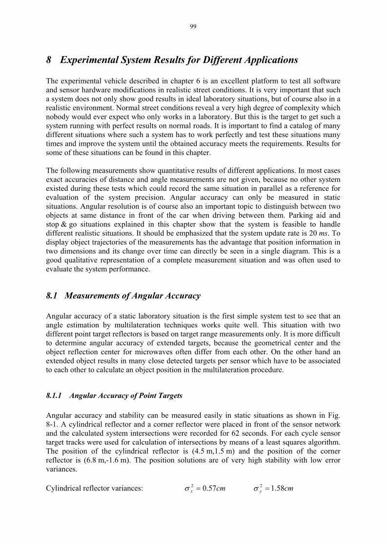
99

8 Experimental System Results for Different Applications The experimental vehicle described in chapter 6 is an excellent platform to test all software and sensor hardware modifications in realistic street conditions. It is very important that such a system does not only show good results in ideal laboratory situations, but of course also in a realistic environment. Normal street conditions reveal a very high degree of complexity which nobody would ever expect who only works in a laboratory. But this is the target to get such a system running with perfect results on normal roads. It is important to find a catalog of many different situations where such a system has to work perfectly and test these situations many times and improve the system until the obtained accuracy meets the requirements. Results for some of these situations can be found in this chapter. The following measurements show quantitative results of different applications. In most cases exact accuracies of distance and angle measurements are not given, because no other system existed during these tests which could record the same situation in parallel as a reference for evaluation of the system precision. Angular accuracy can only be measured in static situations. Angular resolution is of course also an important topic to distinguish between two objects at same distance in front of the car when driving between them. Parking aid and stop & go situations explained in this chapter show that the system is feasible to handle different realistic situations. It should be emphasized that the system update rate is 20 ms. To display object trajectories of the measurements has the advantage that position information in two dimensions and its change over time can directly be seen in a single diagram. This is a good qualitative representation of a complete measurement situation and was often used to evaluate the system performance.

8.1 Measurements of Angular Accuracy Angular accuracy of a static laboratory situation is the first simple system test to see that an angle estimation by multilateration techniques works quite well. This situation with two different point target reflectors is based on target range measurements only. It is more difficult to determine angular accuracy of extended targets, because the geometrical center and the object reflection center for microwaves often differ from each other. On the other hand an extended object results in many close detected targets per sensor which have to be associated to each other to calculate an object position in the multilateration procedure.

8.1.1 Angular Accuracy of Point Targets Angular accuracy and stability can be measured easily in static situations as shown in Fig. 8-1. A cylindrical reflector and a corner reflector were placed in front of the sensor network and the calculated system intersections were recorded for 62 seconds. For each cycle sensor target tracks were used for calculation of intersections by means of a least squares algorithm. The position of the cylindrical reflector is (4.5 m,1.5 m) and the position of the corner reflector is (6.8 m,-1.6 m). The position solutions are of very high stability with low error variances. Cylindrical reflector variances: cmx 57.02 =σ cmy 58.12 =σ

100

Corner reflector variances: cmx 3.02 =σ cmy 67.12 =σ

CylindricalReflector(4.5,1.5)

CornerReflector(6.8,-1.6)

VehicleBumper

Fig. 8-1: Static multiple object situation

Fig. 8-2: Cylindrical reflector and corner reflector

Another measurement to prove angular accuracy of the radar network is depicted in Fig. 8-3. An oil barrel of approximately 40 cm diameter was moved on ±2 m from the vehicle center line and at 8 m in front of the car in a rectangular way. The complete rectangle was moved twice and the sensor network object map was recorded. It is very impressive that on both laps the object map results are very identical. Fig. 8-3 is the plot of the object trajectory in a bird view display, i.e. the picture was not cleared during the measurement. The object position of the complete measurement is visualized. Differences from the ±2 m lines on the sides are systematic errors and reproducible. The maximum deviation to the sides is always less than 50 cm. This example also illustrates that small errors of the measured sensor ranges may result in significant errors of the estimated object position due to the short baseline between the sensors in the bumper. The barrel was moved with a velocity of approximately 15 - 20 cm per second. The four small squares below the measured curve indicate the four sensors mounted in the vehicle bumper.

101

Fig. 8-3: Trajectory of a rectangular movement of an oil barrel (two laps)

The situation in Fig. 8-4 and Fig. 8-5 is a static situation in a corner of a building. The corners in the building wall (marked by 1…3) are like small corner reflectors and can be seen as point targets in the measurements. The door in front of the experimental car is another good reflector in this situation. Displayed results of the radar decision unit are shown on an online display in the car (see Fig. 8-5). The small squares are detected targets of the four sensors displayed directly in front of the specific sensor because a single target of a sensor has only range and no angle information. The arcs indicate sensor target tracks of the individual sensors. These sensor target tracks are used for the multilateration procedures. After target track to target track association a least squares algorithm estimates an object position for the current cycle, i.e. intersection marked by small yellow dots in the display. The bigger red dots are the filtered intersections, i.e. object positions. Fig. 8-5 shows that the three building corners are well detected by the sensors and the angle estimation works quite well. Additionally the door in front of the car is located in the correct position by the multilateration procedures.

102

Fig. 8-4: Static multiple object situation

1

2

3

4

Fig. 8-5: Bird view of the calculated static multiple object situation

103

8.1.2 Angular Accuracy of Extended Targets Extended obstacles include several reflecting centers which are distributed very closely on the vehicle surface. This might e.g. be the rear end of the car in Fig. 8-7 or may result from reflections from the bottom of the car. It is obvious that numerous targets for each sensor will be detected in such a situation and all these targets have to be tracked. Individual sensor target tracks are associated to each other to find a correct object position. If this important track to track association fails, the angle estimation results in a wrong interpretation of the situation. This fact is independent from the kind of processing that is chosen, i.e. a least squares processing and a Kalman filter both can only give good results if the sensor track to track association is correct. The intention of the following results is to show that angle estimation not only of point targets, but also of extended targets is possible. Of course a correct angle estimation of extended obstacles is still a challenging topic for radar networks of this kind, but the results of this work already show some good news that it is not impossible to handle these situations with such a network. Two different distances of the own experimental vehicle’s center axis to the car parked on the side of the street were selected and the distances of the car parked on the side to the center axis were calculated in short measurements. The first measurement was 450 cycles long (9 seconds) and the results are displayed in Fig. 8-7 together with a photograph of the situation from the driver’s seat (Fig. 8-6). Fig. 8-7 shows that the distance to the vehicle center axis is about 1.5 m. In Fig. 8-8 the car parked on the side is about 3 m away from the vehicle center axis. This can also be seen in the diagram (Fig. 8-9). The situation was recorded for 600 cycles, i.e. 12 seconds. It can be seen that the curve in Fig. 8-9 is not as stable as in Fig. 8-7 due to the fact that the sensor on the outer left corner is detecting the car not as good as before. If only three sensors detect the car, the results are not as precise as with four sensors detecting it.

104

Fig. 8-6 Vehicle at 1.5 m from own vehicle axis

0 1 2 3 4 5 6 7 8 9-10

-8

-6

-4

-2

0

2

4

6

8

10

Time [s]

Mea

sure

d di

stan

ce fr

om o

wn

vehi

cle

axis

[m]

Vehicle at 1.5m from own vehicle axis

Fig. 8-7: Measured distance of vehicle at 1.5 m from own vehicle axis

105

Fig. 8-8: Vehicle at 3 m from own vehicle axis

0 2 4 6 8 10 12-10

-8

-6

-4

-2

0

2

4

6

8

10

Time [s]

Mea

sure

d di

stan

ce fr

om o

wn

vehi

cle

axis

[m]

Vehicle at 3m from own vehicle axis

Fig. 8-9: Measured distance of vehicle at 3 m from own vehicle axis

106

8.2 Measurements of Angular Resolution It is not easy to distinguish between two objects with very short distance between each other and at almost the same distance to the vehicle. Even if the range resolution of the single sensor is very high to separate two targets, the data association in the multilateration processor has to be very good to associate the targets correctly to each other to identify the two objects at their correct positions. One test with the vehicle driving between two corner reflectors at the same distance to the vehicle located on ±2 m to the sides is shown in Fig. 8-10.

Fig. 8-10: Trajectory when driving between two corner reflectors

107

8.3 Parking Aid Situations For parking aid situations it is of course important to detect another parked car with high accuracy almost down to distance zero. Furthermore it is very important that a person can be detected with very high probability. One example can be a child running in front of a parking car. The driver could oversee a person easily, but the radar should not. Usually a person is a reflector of very low radar cross section compared with a car, a wall or a metal pole. This measurement shows that the system is well capable to detect and to track a person well up to a distance of approximately 8 m. Fig. 8-11 shows the trajectory of a person walking in front of the car from the left side and walking slowly up to 8 m straight in front of the car. The sensitivity of the sensors is good enough to detect the person up to a maximum distance of 8 m with very precise angle estimation results of the multilateration. Only small errors can be observed.

Fig. 8-11: Trajectory of a person walking in front of the car

108

8.4 Stop & Go Situations The surrounding of a vehicle driving at e.g. 50 km/h is very dynamic and targets for each single sensor appear only for a short time. Targets have to be picked up by the tracker very fast to ensure fast reactions of the system in case of an unavoidable accident. So the use of a radar network in stop & go situations requires detection and tracking of all objects with very precise coordinates. This is a very challenging task concerning the angle estimation. With the experimental vehicle measurements were recorded on normal streets in Hamburg and also on highways at very high speed. For the existing system status a maximum relative velocity to pick up a target for tracking is limited to 50 km/h by the gate for target to track association. For first feasibility tests this limitation was accepted. For higher relative velocities the data association has to be improved. Fig. 8-12 shows a situation where a lamp pole on the side of the street was passed in a curve. Such a lamp pole is like a cylindrical reflector of very small radar cross section due to the small diameter. So as a point target it is easy to estimate an object position for these lamp poles on the street sides. They can often be observed in measurements and always tracked with high precision of distance and angle. In Fig. 8-13 the trajectory of the lamp is depicted. The object was first picked up at 14 m. Passing parked cars is an important task when driving in a town. The system has to be able to locate the parked objects on the side and not on the road. For an error in position finding, an ACC car would immediately activate the brakes which may cause a dangerous situation for other following drivers on this road. Fig. 8-14 shows the situation and Fig. 8-15 shows the object trajectories when passing the parked cars. Velocity was not more than 20 km/h. The precision of an angle estimation of these extended objects is not as good as in the case of a point target especially when a car is measured from this aspect angle. Pointing with the radar at the vehicle corner, the side of the vehicle is like a mirror, reflecting emitted energy away from the radar sensor. The same does the back of the car from this aspect angle. A real stop & go situation is depicted in Fig. 8-16. The object radius for this situation is shown in Fig. 8-17. The diagram shows radial distance versus cycles (1 cycle equals 20 ms). The vehicle in front of the experimental car is seen as an object with slowly changing distance between 18 m and 10 m. Passed objects (i.e. cars parked on the side) are seen as very steep lines in the diagram. The distance changes very fast. Own velocity can be estimated from the gradient of the lines. Fig. 8-18 shows the corresponding estimated angles in degrees over cycles. For the car in front a precise angle was estimated around zero degrees. Passed objects are first seen at small angles at higher distance. With smaller distance these objects move relative to the own car from the center to the side when being passed. So the angle increases for objects being passed. Most fixed objects are detected on the right side (negative angle). From range rate estimation Fig. 8-19 shows relative velocity in x-direction (m/s over cycles). For the objects appearing for a very short time the velocity estimation is not as precise as for the car in the front. Fig. 8-20 and Fig. 8-21 are presented to show an example of the results of the single sensor target tracking. Fig. 8-20 shows the targets detected in each single cycle by the outermost right sensor. The single sensor target tracker has the task to extract relevant information from this picture in each single cycle. Fig. 8-21 is what the target tracker extracted and tracked from the detected target lists. The vehicle in the front was always detected with very high probability of detection and also many fixed objects were picked up and tracked by this sensor. So the target tracker really extracted the most important information from all the data.

109

Fig. 8-12: Street lamp pole in a curve

Fig. 8-13: Trajectory when passing a street lamp pole

110

Fig. 8-14: Passing parked cars

Fig. 8-15: Trajectories of two passed cars

111

Fig. 8-16: Stop & Go situation

Fig. 8-17: Object radius of stop & go situation (radius [m] vs. cycles (time))

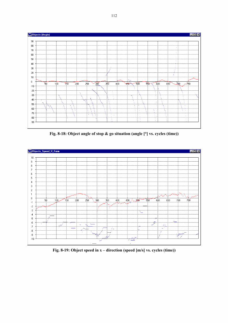
112

Fig. 8-18: Object angle of stop & go situation (angle [°] vs. cycles (time))

Fig. 8-19: Object speed in x – direction (speed [m/s] vs. cycles (time))

113

Fig. 8-20: Target detections of sensor 4 (right vehicle side, range [m] vs. cycles (time))

Fig. 8-21: Sensor target tracks of sensor 4 (range [m] vs. cycles (time))

114

8.5 Blind Spot Surveillance Blind spot surveillance is merely a presence detection to the vehicle sides. Due to the fact that the experimental vehicle was not modified for this application, no practical results can be presented at this place. Target detection in the short range up to e.g. five meters to the vehicle sides with high range accuracy is without any doubt possible with the used sensors. Numerous measurements in the laboratory to improve single sensor detection and range measurement algorithms underline the feasibility of this application.

115

9 Conclusion This thesis presented a system description of a radar sensor network based on recently developed high range resolution radar technology at 24 GHz. With range measurement of very high accuracy with each individual sensor in the radar network, the data fusion and tracking is based on multilateration techniques. Angle estimation mainly accomplished by range measurement of high accuracy is very well possible with the used sensor technology. Requirements for the accuracy to be achieved with each sensor was evaluated in chapter 2. Chapter 3 presented important topics of single sensor signal processing along with a description of the implemented measurement principle. Although the system results of chapter 8 are based on range measurement only, a simultaneous range and velocity measurement is also possible, but not yet introduced into the complete network. Ideas for simultaneous measurement of range and velocity are explained in chapter 3 with results in chapter 7. The radar network processing requires very elaborated data association algorithms. Improvement at this point beyond the current status described in chapter 4 is still possible. The implemented multilateration described in chapter 4 is based on least squares position estimation and Kalman filtering and showed good results in measurements and simulations. Modifications of the sensor concept can additionally bring some tremendous progress and may also relieve the difficulties of perfect data association, because with the suggested concept of a phase monopulse sensor explained in chapter 5 an angle estimation by phase measurement with a single sensor is possible. With the presented extended Kalman filter the redundancy can be used to achieve very precise results for angle estimation. An implementation of such a radar network in a normal passenger car is surely a highlight of this thesis, because practical experiences are worth much more than only theoretical evaluation of system feasibility. The experimental vehicle is an excellent platform for tests in a real world environment and was extensively used for further improvements. Development of such a radar network makes no sense without directly measuring the system performance in realistic street conditions. Fast progress in the development of such a radar network is only possible with experimental experience. As a conclusion it is important to notice that the development of automotive radar networks based on 24 GHz and 77 GHz sensor technology is surely not finished with this work. Main objectives of this thesis are to show feasibility of basic functionality and that such a radar network is well suited for the suggested applications. A first step is done and requires to be followed by further investigation. Of all possible sensor technologies available today, radar technology has many advantages and will surely be a candidate for automotive safety and comfort applications in the next years. The results of this thesis should encourage to spend additional effort in further development to improve the system for more difficult situations. Apart from the range measurement being already of an astonishing precision, it should not be concealed that perfect angle estimation is still an interesting challenge for the future as well as further testing and improvement in more dynamic situations.

116

117

Appendix

A Standard Form of the Radar Equation Power density at distance R:

24density Power

RGPT

π= (A-1)

with: : transmit power R: distance G: antenna gain TP Isotropic reflected power from target at distance R:

24power Reflected

RGPT

πσ

= (A-2)

with: G: antenna gain σ: effective area of isotropic target

Reflected power density back at the radar:

( )224

density power ReflectedR

GPT

π

σ= (A-3)

Basic radar equation (e.g. [LEV88]):

( ) 43

22

4 RGPP T

R πσλ

= with: πλ

4

2GA = : effective receiving antenna area (A-4)

: received power RP The effective area of the isotropic target is also called its radar cross section. This is the area of a target that reflects back isotropically and would have caused the same return power as the original target. The radar cross section is usually very different from the physical dimensions of a target. Other form of the radar equation (see e.g. [LUD98]):

( ) atmtnsys

t

aus LLBkTRGP

NS

⋅⋅

⋅⋅=

1

4 43

22

πσλ

(A-5)

with: : noise power nsys BTkN ⋅⋅=

: losses due to the distance between transmitter and antenna tL : losses due to atmospheric attenuation atmL

118

B Basic Equations for Single Pulse Detection The output signal without noise can be described by:

(B-1)

( ) ( ) ( ) ( )tbtatAts ccsc ωωϕω sincoscos0 ⋅+⋅=−⋅=

ccs fabbaA πωϕ 2 ;arctan ;22 =

=+=

The output noise of the receiver can be described by:

(B-2) ( ) ( ) ( ) ( ) ( )ttYttXtn cc ωω sincos0 +=

with being the center frequency and X(t), Y(t) are independent random variables with Gaussian probability density function, zero average and same variance.

cω

The combined output of signal and noise gets:

( ) ( ) ( ) ( )[ ] ( ) ( )[ ] ( ) ( ) ( )( )tttrttYbttXatntste ccc ϕωωω +=+++=+= cossincos000

(B-3)

with: ( ) ( )[ ] ( )[ ] ( ) ( )tYtXtYbtXatr 21

21

22 +=+++= ( ) ( )( )

++

=tXatYbt arctanϕ

The probability density functions of both parts assuming independent Gaussian variables are as follows:

( ) ( )

−−= 2

21

11 2exp

21

NN

aXXp

σπσ and ( ) ( )

−−= 2

21

12 2exp

21

NN

bYYp

σπσ (B-4)

Due to independence from each other the two-dimensional joint probability density function is the product of both parts:

( ) ( ) ( ) ( ) ( )

−+−=⋅= 2

21

21

2121111 2exp

21,

NN

bYaXYpXpYXpσπσ

(B-5)

The transformation to polar coordinates (r, ϕ) can be achieved with the relations:

( )ϕcos1 rX = ( )ϕsin1 rY = 21

21 YXr +=

=

1

1arctanXY

ϕ

(B-6)

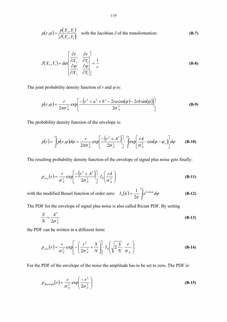
119

( ) ( )( )11

11

,,,YXJYXprp =ϕ with the Jacobian J of the transformation: (B-7)

( )r

YX

Yr

Xr

YXJ 1det,

11

1111 =

∂∂

∂∂

∂∂

∂∂

= ϕϕ (B-8)

The joint probability density function of r and ϕ is:

( ) ( ) ( )( )

−−++−= 2

222

2 2sin2cos2exp

2,

NN

rbrabarrrpσ

ϕϕπσ

ϕ (B-9)

The probability density function of the envelope is:

( ) ( ) ( ) ( ) ϕϕϕσσπσ

ϕϕππ

drAArrdrprp sNNN

−⋅⋅

+−== ∫∫ cosexp

2exp

2, 2

2

02

22

2

2

0

(B-10)

The resulting probability density function of the envelope of signal plus noise gets finally:

( ) ( )

⋅

+−= 202

22

2 2exp

NNNrice

rAIArrrpσσσ

(B-11)

with the modified Bessel function of order zero: ( ) ∫ ⋅=π

ϕ ϕπ

2

0

cos0 2

1 dekI k (B-12)

The PDF for the envelope of signal plus noise is also called Rician PDF. By setting

2

2

2 N

ANS

σ= (B-13)

the PDF can be written in a different form:

( )

⋅⋅

+−=

NNNrice

rNSI

NSrrrp

σσσ2

2exp 02

2

2 (B-14)

For the PDF of the envelope of the noise the amplitude has to be set to zero. The PDF is:

( )

−= 2

2

2 2exp

NNRayleigh

rrrpσσ

(B-15)

120

C FFT Memory and Timing Requirement For the processing of Fourier Transforms, the processing hardware performance plays an important role. For a standard FFT library for the TMS320C2000 digital signal processor family the memory requirements and the timing requirements are listed below to get an overview of what is feasible with cheap processor hardware of limited performance. The processors are 16 bit fixed-point processors running at 20 MHz. Data is taken from [TEX98]. The forward FFT memory requirements are:

Program Memory Words

FFT Size

Data Memory Words for intermediate storage

Function Size Sine Table Size

N 2N+17 ¾ N 32 81 109 24 64 145 109 48

128 273 109 96 256 529 114 192 512 1041 114 384

1024 2065 114 768

Table C-0-1: Forward FFT Memory Requirements

The forward FFT timing requirements are:

FFT Size Clock Cycles Time[ms] (20MHz) Time[ms] (40MHz) N O(N*logN) O(N*logN) O(N*logN) 32 7.552 0.3776 0.1888 64 17.216 0.8608 0.4304

128 38.880 1.944 0.9720 256 86.298 4.315 2.157 512 238.016 11.90 5.950

1024 522.720 26.14 13.07

Table C-0-2: Forward FFT Timing Requirements

121

D Resolution of Doppler Ambiguities As already described in chapter 3.2.3.2, the true frequency to be calculated for the ambiguous measured real values and is: '

1M '2M

222111 MfVMfVM ′+⋅=′+⋅= (D-1)

The solutions for the numbers of the ambiguous intervals V1 and V2 are the interesting values. The two chosen ramp frequencies f1 and f2 have to be two numbers with no common divisor. First both measured values have to be normalised:

10 ; 10 ; 22

221

1

11 ≤≤

′=≤≤

′= M

fM

MMf

MM (D-2)

(D-1) is then:

( ) ( 222111 fMVfMVM +=+= )

( ) ( ) 0 222111 =+−+⇒ fMVfMV (D-3)

Both frequency intervals f1 and f2 can be divided into J1 and J2 subsections. The numbers J1 and J2 have no common divisor. This results:

12212

1

2

1 JfJfJJ

ff

=⇒= (D-4)

The subsections have all the same length E:

2

2

1

1

Jf

Jf

E == (D-5)

With (D-4) equation(D-3) becomes:

(D-6) ( ) ( ) ( ) ( ) 0 0 11221122222111 =−+−⇒=+−+ JVJVJMJMJMVJMV

The first term of (D-6) is known and the second term includes the unknown values V1 and V2. With the following substitution the equation is:

( ) ( ZJVJVJMJMZ =−⇒−= 22111122 )

)

(D-7)

with: (D-8) ( ) ( 11 21 −≤≤−− JZJ

After some steps the solution is (see [ROH86] for a detailed derivation):

122

( ) ( )( )( 211 mod1 JZVZV = )) (D-9)

( ) ( )( )( 122 mod1 JZVZV = (D-10)

with:

( ) ( ) ( ) ( )21

211 mod1 2 JJJV J −−= ϕ (D-11)

( ) ( ) ( ) ( )11

212 mod1 1 JJJV J −−= ϕ (D-12)

ϕ(m) is Euler’s function [SCH90] defined as the number of positive integers r smaller than m that are coprime to m, i.e., for which 1 ≤ r < m. Note: ϕ(1) = 1; If m is prime, ϕ(m) is: ϕ(m) = m − 1. Example: m = 10; r = 1,3,7,9. Thus ϕ(10) = 4. m = 11; ϕ(11) = 10. The solution can be checked with: ( ) ZJVJV =− 2211

A flow chart of the algorithm is shown in Fig. D-0-1.

Measurement

Normalization:M1 = M1' / f1M2 = M2' / f2

Calculation of Z:Z = M2J2 - M1J1

V1(Z), V2(Z)True frequency:M = [M1+V1(Z)]f1 = [M2+V2(Z)]f2

V1(1), V2(1)

M1', M2'

M

Resolution algorithm

Fig. D-0-1: Resolution of Doppler ambiguities

123

References [BAR88] Bar-Shalom, and T. E. Fortmann: “Tracking and Data Association“, Orlando,

FL, Academic Press, 1988. [BAR93] Bar-Shalom, Y. and Li, Xiao-Rong: “Estimation and Tracking – Principles,

Techniques and Software”, Norwood MA, Artech House, 1993. [BRI74] Brigham, E. Oran: “The Fast Fourier Transform”, Prentice Hall, Inc.,

Englewood Cliffs, N.J., 1974. [BLA86] Blackman, S.: “Multiple-Target Tracking with Radar Applications”, Dedham

MA, Artech House, 1986. [BLA99] Blackman, S., and Popoli, R.: “Design and Analysis of Modern Tracking

Systems”, Norwood MA, Artech House, 1999. [BRO] Bronstein-Semendjajew: “Taschenbuch der Mathematik”, Teubner, 24.

Auflage. [BRO98] Brookner, Eli: “Tracking and Kalman Filtering Made Easy”, John Wiley &

Sons, 1998. [BRO97] Brown, R. G.: “Introduction to Random Signals and Applied Kalman

Filtering”, John Wiley & Sons, 1997. [CHU81] Churchill, F.E.; Ogar, G. W.; Thompson, B. J.: “The Correction of I and Q

Errors in a Coherent Processor”, IEEE Transactions on Aerospace and Electronic Systems, Vol. AES-17, No. 1, pp. 131, January 1981.

[ERI95] Eriksson, L. H. and As, B. O.: “A High Performance Automotive Radar for

Automatic AICC”, IEEE International Radar Conference, Alexandria, Virginia, May 1995.

[ETS00] Etschberger, K.: “Controller Area Network“; Carl Hanser Verlag, Munich, 2nd

Edition, 2000. [HAA00] Haas, G.: “Datenzuordnungsverfahren in einem Automobil - Radarnetzwerk”;

Diploma Thesis, TU Hamburg-Harburg, Department of Telecommunications, 2000.

[HAN00] Hansen, M.: “Entwicklung eines Systems zur automatischen Kalibrierung von

KFZ – Nahbereich – Radarsensoren”; Diploma Thesis, TU Hamburg-Harburg, Department of Telecommunications, 2000.

[IEEE96] Institute of Electrical and Electronics Engineers, Inc.: “The IEEE Standard

Dictionary of Electrical and Electronics Terms“, 6th Edition, IEEE Std 100-1996

124

[KLO99] Klotz, M. and Rohling, H.: “A High Range Resolution Radar System Network for Parking Aid Applications”, 5th International Conference on Radar Systems 1999, Brest, France, May 1999.

[KLO00] Klotz, M. and Rohling, H.: “24 GHz Radar Sensors for Automotive

Applications”, 13th International Conference on Microwaves, Radar and Wireless Communications, Poland, Wroclaw, May 22-24, 2000.

[KUH00] Kuhlmann, V.: “Entwurf und Performanceanalyse eines Bussystems für

sicherheitsrelevante Anwendungen mit verteilten Radarsensoren im Automobil“; Studienarbeit, TU Hamburg-Harburg, Department of Tele-communications, 2000.

[LAY97] Lay, David C.: “Linear Algebra and its Applications”; 2nd Edition, Addison

Wesley, 1997. [LEV88] Levanon, Nadav: “Radar Principles”; John Wiley & Sons Inc., 1988. [LUD98] Ludloff, A.: “Praxiswissen Radar und Radarsignalverarbeitung”, Vieweg

Verlag, 2. Auflage, 1998. [MEI01] Meinecke, M.-M.: “Zum optimierten Sendesignalentwurf für Automobil-

radare”; PhD Thesis, TU Hamburg-Harburg, Department of Telecommunications, 2001.

[MEN99] Mende, R.: “Radarsysteme zur automatischen Abstandsregelung in

Automobilen”; PhD Thesis, TU Braunschweig, 1999. [MEN00] Mende, R.; Zander, A.: “A Multifunctional Automotive Short Range Radar

System”, German Radar Symposium, GRS2000, Berlin, October 10-11, 2000. [REE98] Reed, J. C.: “Side Zone Automotive Radar”; IEEE AES Systems Magazine,

pp. 3-7, June 1998. [REI79] Reid, D. B.: “An Algorithm for Tracking Multiple Targets“; IEEE

Transactions on Automatic Control, Vol. AC-24, Dec. 1979, pp. 843-854. [ROH83] Rohling, H.: “Radar CFAR Thresholding in Clutter and Multiple Target

Situations“; IEEE Transactions on Aerospace and Electronic Systems, Vol. AES-19, No. 4, July 1983.

[ROH86] Rohling, H.: “Zur Auflösung von Radialgeschwindigkeits- und Entfernungs-

mehrdeutigkeiten bei der Radarmessung“; ntzArchiv Bd. 8 (1986), H. 2. [ROT90] Rottler, J.: “Auflösung von Geschwindigkeits- und Entfernungsmehrdeutig-

keiten beim Puls-Radar“; PhD Thesis, Karlsruhe 1990. [SCH90] Schroeder, M. R.: “Number Theory in Science and Communication“; Springer

Verlag, 1990.

125

[TEX98] Texas Instruments, Application Report SPRA354: “TMS320C2000 C-callable FFT package”, May 1998.

[ULK94] Ulke, W.; Adomat, R.; Butscher, K.; Lauer, W.: “Radar – based Automotive

Obstacle Detection Systems”; SAE Technical Paper Series, International Congress & Exposition, Michigan 1994.

[WAG97] Wagner, Klaus-Peter: “Winkelauflösende Radarverfahren für Kraftfahrzeug-

anwendungen”; PhD Thesis, TU Munich, Lehrstuhl für Hochfrequenztechnik, 1997.

[WEI98] Weidmann, W. and Steinbuch, D.: “A High Resolution Radar for Short Range

Automotive Applications”; 28th European Microwave Conference 1998, Amsterdam, pp. 590-594.

[WEN00] Weng, W.: “Programmierung einer graphischen Anzeige mit hoher

Updaterate unter MS Windows für ein KFZ - Radarsystem”; Diploma Thesis, TU Hamburg-Harburg, Department of Telecommunications, 2000

126

127

Acronyms and Abbreviations

ACC Adaptive Cruise Control CA Collision Avoidance CA-CFAR Cell-Averaging Constant False Alarm Rate CAGO-CFAR Cell-Averaging Greatest Of Constant False Alarm Rate CAN Controller Area Network CFAR Constant False Alarm Rate DFT Discrete Fourier Transform DRO Dielectric Resonator Oscillator DSP Digital Signal Processor ECU Electronic Control Unit FFT Fast Fourier Transform FMCW Frequency Modulated Continuous Wave HPRF High Pulse Repetition Frequency HRR High Range Resolution IF Intermediate Frequency ISM Industrial, Scientific, Medical JPDA Joint Probabilistic Data Association LO Local Oscillator LPRF Low Pulse Repetition Frequency MHT Multiple Hypothesis Tracking MOST Media Oriented Systems Transport MPRF Medium Pulse Repetition Frequency OS-CFAR Ordered-Statistic Constant False Alarm Rate PDA Probabilistic Data Association PDF Probability Density Function PRF Pulse Repetition Frequency PRI Pulse Repetition Interval RADAR Radio Detection and Ranging RDU Radar Decision Unit RF Radio Frequency SRD Step Recovery Diode TDMA Time Division Multiple Access TTP Time-Triggered Protocol

128

129

List of Figures Fig. 2-1: Sensor network with four subsystems monitoring the complete car environment...... 4 Fig. 2-2: Applications of an automotive short range radar network and percentage of accidents

from different directions..................................................................................................... 5 Fig. 2-3: Network implementation in the experimental vehicle................................................. 6 Fig. 2-4: Multilateration situation with a single object ............................................................ 11 Fig. 2-5: Error of object angle using only two sensors ............................................................ 12 Fig. 2-6: Lateral distance error as a function of longitudinal and angle error.......................... 12 Fig. 2-7: Lateral distance error as a function of angle error..................................................... 13 Fig. 2-8: Sensor network accuracy with distance errors up to ±10cm of only two sensors ..... 13 Fig. 2-9: Bumper geometry ...................................................................................................... 14 Fig. 2-10: Standard deviation of the calculated angle with variable target distance to the

vehicle center axis ............................................................................................................ 15 Fig. 3-1: Signal Processing of a Pulse Radar ........................................................................... 18 Fig. 3-2: 24 GHz sensor hardware structure ............................................................................ 20 Fig. 3-3: Example of a sensor delay sweep signal and sensor frontend................................... 20 Fig. 3-4: Laboratory situation of two close objects.................................................................. 22 Fig. 3-5: Probability density functions of noise and signal...................................................... 25 Fig. 3-6: Processing of an OS-CFAR detector......................................................................... 26 Fig. 3-7: FFT length versus velocity resolution and measurement time versus velocity

resolution.......................................................................................................................... 28 Fig. 3-8: Doppler frequency resolution as a function of the required velocity resolution ....... 28 Fig. 3-9: Processing with stepped ramps.................................................................................. 29 Fig. 3-10: Processing with staggered ramp duration................................................................ 30 Fig. 3-11: Doppler frequency resolution .................................................................................. 32 Fig. 3-12: Range Resolution as a Function of Pulse Width and Frequency Hub..................... 34 Fig. 3-13: SNR versus PD for single pulse detection (Source: [LEV88]) ................................ 37 Fig. 3-14: Transmit pulse width versus distance and increase of signal-to-noise ratio versus

distance............................................................................................................................. 38 Fig. 3-15: Example of sensor interference ............................................................................... 39 Fig. 3-16: Transmit and receive pulses of four sensors............................................................ 39 Fig. 3-17: PRF-oscillator detuning for interference suppression ............................................. 42 Fig. 4-1: Coordinate system ..................................................................................................... 46 Fig. 4-2: System architecture 1 ................................................................................................ 47 Fig. 4-3: System architecture 2 ................................................................................................ 47 Fig. 4-4: Central-level tracking with centralized processing ................................................... 48 Fig. 4-5: Sensor-level tracking with centralized track file ....................................................... 49 Fig. 4-6: Example of an estimated object position by means of a least squares algorithm...... 50 Fig. 4-7: Error of azimuth angle (system with four and six sensors) ....................................... 54 Fig. 4-8: Angle error for variable number of sensors............................................................... 54 Fig. 4-9: Processing of the Kalman filter ................................................................................. 57 Fig. 4-10: Object radius error and angle error for Kalman filter and least squares solution.... 60 Fig. 4-11: Object velocity in x – and y – direction (Kalman filter) ......................................... 60 Fig. 4-12: Abstract Data Fusion Model.................................................................................... 61 Fig. 4-13: Generalised Processing Overviews (α - β - Tracker and Kalman Filter)................ 63 Fig. 4-14: Target to track data association ............................................................................... 64 Fig. 4-15: Measurement-oriented MHT algorithm .................................................................. 67 Fig. 4-16: Track-oriented MHT algorithm............................................................................... 69 Fig. 4-17: Radar network processing overview ....................................................................... 72

130

Fig. 5-1: Frontend of the phase monopulse sensor................................................................... 74 Fig. 5-2: Object angle error vs. phase error.............................................................................. 74 Fig. 5-3: Wavefront reconstruction with a phase monopulse concept ..................................... 74 Fig. 5-4: Block diagram of the sensor concept......................................................................... 75 Fig. 5-5: Data Fusion Overview............................................................................................... 76 Fig. 5-6: Extended Kalman Filter Processing .......................................................................... 81 Fig. 5-7: Object radius error and angle error for extended Kalman filter ................................ 82 Fig. 5-8: Object velocity in x – and y – direction for extended Kalman filter ......................... 82 Fig. 6-1: Short range sensor network integrated in a vehicle front bumper............................. 86 Fig. 6-2: Experimental vehicle equipment ............................................................................... 86 Fig. 6-3: RDU industrial PC with data acquisition CAN board and DSP hardware................ 88 Fig. 6-4: Radar Decision Unit Overview ................................................................................. 88 Fig. 6-5: Online display in the driver’s cockpit ....................................................................... 89 Fig. 6-6: Block diagram of a closed-loop adaptive cruise control ........................................... 91 Fig. 7-1: Automatic sensor test system block diagram ............................................................ 94 Fig. 7-2: Equipped carrier rail vehicle ..................................................................................... 94 Fig. 7-3: Configuration for RDU angle accuracy measurements............................................. 95 Fig. 7-4: Configuration for distance accuracy and stability measurements versus temperature

.......................................................................................................................................... 95 Fig. 7-5: Single sensor range accuracy..................................................................................... 96 Fig. 7-6: Sequence at time step 1273 and spectrum at 14.8m.................................................. 98 Fig. 7-7: Sequence at time step 1275 (200 ms later) and spectrum at 12.9m .......................... 98 Fig. 7-8: Sequence at time step 1277 (200 ms later) and spectrum at 11.2m .......................... 98 Fig. 8-1: Static multiple object situation ................................................................................ 100 Fig. 8-2: Cylindrical reflector and corner reflector ................................................................ 100 Fig. 8-3: Trajectory of a rectangular movement of an oil barrel (two laps)........................... 101 Fig. 8-4: Static multiple object situation ................................................................................ 102 Fig. 8-5: Bird view of the calculated static multiple object situation .................................... 102 Fig. 8-6 Vehicle at 1.5 m from own vehicle axis ................................................................... 104 Fig. 8-7: Measured distance of vehicle at 1.5 m from own vehicle axis................................ 104 Fig. 8-8: Vehicle at 3 m from own vehicle axis ..................................................................... 105 Fig. 8-9: Measured distance of vehicle at 3 m from own vehicle axis................................... 105 Fig. 8-10: Trajectory when driving between two corner reflectors........................................ 106 Fig. 8-11: Trajectory of a person walking in front of the car................................................. 107 Fig. 8-12: Street lamp pole in a curve .................................................................................... 109 Fig. 8-13: Trajectory when passing a street lamp pole .......................................................... 109 Fig. 8-14: Passing parked cars................................................................................................ 110 Fig. 8-15: Trajectories of two passed cars.............................................................................. 110 Fig. 8-16: Stop & Go situation ............................................................................................... 111 Fig. 8-17: Object radius of stop & go situation (radius [m] vs. cycles (time)) ...................... 111 Fig. 8-18: Object angle of stop & go situation (angle [°] vs. cycles (time)) .......................... 112 Fig. 8-19: Object speed in x – direction (speed [m/s] vs. cycles (time)) ............................... 112 Fig. 8-20: Target detections of sensor 4 (right vehicle side, range [m] vs. cycles (time))..... 113 Fig. 8-21: Sensor target tracks of sensor 4 (range [m] vs. cycles (time)) .............................. 113 Fig. D-0-1: Resolution of Doppler ambiguities ..................................................................... 122

131

List of Tables Table 2-1: Suggested realistic system requirements for different applications ......................... 9 Table 3-1: Main sensor features ............................................................................................... 21 Table 4-1: Example of an assignment matrix........................................................................... 65 Table 6-1: Obstacle movement for different velocities............................................................ 91 Table C-0-1: Forward FFT Memory Requirements ............................................................... 120 Table C-0-2: Forward FFT Timing Requirements ................................................................. 120

Lebenslauf Name: Michael Klotz Geburtsdatum: 16.08.1971 Geburtsort: Ungeny / Moldawien Schulbildung: 1977 – 1981: Grundschule in Hildesheim und in Holle (Landkreis Hildesheim) 1981 – 1983: Orientierungsstufe in Bockenem 1983 – 1990: Scharnhorst – Gymnasium in Hildesheim; Abschluss: Abitur Studium:

10/1991 – 12/1996: Studium der Elektrotechnik an der TU Braunschweig mit

Vertiefungsrichtung Meß- Regelungs- und Automatisierungstechnik 11/1995 – 08/1996: Diplomarbeit am Institut für Regelungstechnik der TU Braunschweig 08/1996 – 12/1996: Studienarbeit bei der Firma Aerodata Flugmesstechnik GmbH in

Braunschweig

Berufliche Tätigkeit: 12/1996 – 03/1997: Diplom – Ingenieur in der Abteilung Navigationssysteme bei der Firma

Aerodata Flugmesstechnik GmbH in Braunschweig 04/1997 – 03/1999: wissenschaftlicher Mitarbeiter am Institut für Nachrichtentechnik der

TU Braunschweig im Bereich „Radarsysteme für Automobile“ 04/1999 – 10/2001: wissenschaftlicher Mitarbeiter am Arbeitsbereich Nachrichtentechnik

der TU Hamburg-Harburg im Bereich „Radarsysteme für Automobile“ seit 11/2001: Forschung und Entwicklung automobiler und industrieller Radar-

systeme bei der smart microwave sensors GmbH in Braunschweig (http://www.smartmicro.de)