An Approach to Mapping of Shallow Petroleum Reservoirs

Brigham Young University Brigham Young University

BYU ScholarsArchive BYU ScholarsArchive

Theses and Dissertations

2007-11-17

An Approach to Mapping of Shallow Petroleum Reservoirs Using An Approach to Mapping of Shallow Petroleum Reservoirs Using

Integrated Conventional 3D and Shallow P- and SH-Wave Seismic Integrated Conventional 3D and Shallow P- and SH-Wave Seismic

Reflection Methods at Teapot Dome Field in Casper, Wyoming Reflection Methods at Teapot Dome Field in Casper, Wyoming

Anita Onohuome Okojie-Ayoro Brigham Young University - Provo

Follow this and additional works at: https://scholarsarchive.byu.edu/etd

Part of the Geology Commons

BYU ScholarsArchive Citation BYU ScholarsArchive Citation Okojie-Ayoro, Anita Onohuome, "An Approach to Mapping of Shallow Petroleum Reservoirs Using Integrated Conventional 3D and Shallow P- and SH-Wave Seismic Reflection Methods at Teapot Dome Field in Casper, Wyoming" (2007). Theses and Dissertations. 1219. https://scholarsarchive.byu.edu/etd/1219

This Thesis is brought to you for free and open access by BYU ScholarsArchive. It has been accepted for inclusion in Theses and Dissertations by an authorized administrator of BYU ScholarsArchive. For more information, please contact [email protected], [email protected].

http://home.byu.edu/home/

http://home.byu.edu/home/

https://scholarsarchive.byu.edu/

https://scholarsarchive.byu.edu/etd

https://scholarsarchive.byu.edu/etd?utm_source=scholarsarchive.byu.edu%2Fetd%2F1219&utm_medium=PDF&utm_campaign=PDFCoverPages

http://network.bepress.com/hgg/discipline/156?utm_source=scholarsarchive.byu.edu%2Fetd%2F1219&utm_medium=PDF&utm_campaign=PDFCoverPages

https://scholarsarchive.byu.edu/etd/1219?utm_source=scholarsarchive.byu.edu%2Fetd%2F1219&utm_medium=PDF&utm_campaign=PDFCoverPages

mailto:[email protected],%[email protected]

AN APPROACH TO MAPPING SHALLOW PETROLEUM RESERVOIRS USING

INTEGRATED CONVENTIONAL 3D AND SHALLOW P- AND SH-WAVE

SEISMIC REFLECTION METHODS, TEAPOT DOME FIELD,

CASPER, WYOMING

By

Anita Onohuome Okojie-Ayoro

A thesis submitted to the faculty of

Physical and Mathematical Sciences

Brigham Young University

In partial fulfillment of the requirements for the degree of

Masters of Science

Department of Geological Sciences

Brigham Young University

December 2007

ii

BRIGHAM YOUNG UNIVERSITY

GRADUATE COMMITTEE APPROVAL

of a thesis submitted by

Anita Onohuome Okojie-Ayoro

This thesis has been read by each member of the following graduate committee and

by a majority vote has been found to be satisfactory.

______________________ ____________________________________ Date John H. McBride ____________________________ _____________________________________ Date Ron A. Harris ____________________________ _____________________________________ Date Thomas H. Morris

iii

BRIGHAM YOUNG UNIVERSITY

As chair of the candidate’s graduate committee, I have read the thesis of Anita Onohuome Okojie-Ayoro in its final form and have found that (1) its format, citations, and bibliographical style are consistent and acceptable and fulfill university and department style requirements; (2) its illustrative materials including figures, tables, and charts are in place; and (3) the final manuscript is satisfactory to the graduate committee and is ready for submission to the university library. ______________________ ____________________________________ Date John H. McBride Chair, Graduate Committee Accepted for the Department ____________________________________ Scott M. Ritter Department Chair Accepted for the College ____________________________________ Thomas W. Sederberg Associate Dean, College of Physical and Mathematical Sciences

iv

ABSTRACT

AN APPROACH TO MAPPING SHALLOW PETROLEUM RESERVOIRS USING

INTEGRATED CONVENTIONAL 3D AND SHALLOW P- AND SH-WAVE

SEISMIC REFLECTION METHODS, TEAPOT DOME FIELD,

CASPER, WYOMING

Anita O. Okojie-Ayoro

Department of Geological Sciences

Master of Science

Using the famous Teapot Dome oil field in Casper, Wyoming, USA as a test case, we

demonstrate how high-resolution compressional (P) and horizontally polarized shear

(SH) wave seismic reflection surveys can overcome the limitations of conventional

3D seismic data in resolving small-scale structures in the very shallow subsurface (<

100-200 m (~328-656 ft)). We accomplish this by using small CMP intervals (5 ft

and 2.5 ft, respectively) and a higher frequency source. The integration of the two

high-resolution seismic methods enhances the detection and mapping of fine-scale

deformation and stratigraphic features at shallow depth that cannot be imaged by

conventional seismic methods. Further, when these two high-resolution seismic

methods are integrated with 3D data, correlated drill hole logs, and outcrop mapping

and trenching, a clearer picture of both very shallow reservoirs and the relationship

v

between deep and shallow faults can be observed. For example, we show that the

Shannon reservoir, which is the shallowest petroleum reservoir at Teapot Dome

(depth to the top of this interval ranging from 76-198 m (250-650 ft)) can only be

imaged properly with high-resolution seismic methods. Further, northeast-striking

faults are identified in shallow sections within Teapot Dome. The strike of these

faults is approximately orthogonal to the hinge of Teapot Dome. These faults are

interpreted as fold accommodation faults. Vertical displacements across these faults

range from 10 to 40 m (~33 to 131 ft), which could potentially partition the Shannon

reservoir. The integration of 3D and high-resolution P-wave seismic interpretation

helped us determine that some of the northeast-striking faults relate to deeper faults.

This indicates that some deeper faults that are orthogonal to the fold hinge cut

through the shallow Shannon reservoir. Such an observation would be important for

understanding the effect on fluid communication between the deep and shallow

reservoirs via these faults. Furthermore, the high-resolution seismic data provide a

means to better constrain the location of faults mapped from drill hole logs.

Relocation of theses faults may require re-evaluation of well locations as some attic

oil may have not been drained in some Shannon blocks by present well locations.

Therefore our study demonstrates how conventional 3D seismic data require

additional seismic acquisition at smaller scales in order to image deformation in

shallow reservoirs. Such imaging becomes critical in cases of shallow reservoirs

where it is important to define potential problems associated with

compartmentalization of primary production, hazard mitigation, enhanced oil

recovery, or carbon sequestration.

vi

ACKNOWLEDGEMENTS

First of all, I want to extend thanks to my advisor, Dr. John McBride, for his

immense support and contribution not only to this work but to my welfare in general as a

student. I am grateful to Dr. Harris and Dr. Morris for serving as members of my

committee. Thanks to Bill Keach for sharing his knowledge on 3D seismic interpretation.

My thanks go to Kris Mortensen, Marge Morgan and Kim Sullivan for being there

to solve whatever problems I brought before them. I also want to thank Tanner Hicks for

all those days he spent with me editing my figures for this thesis.

My love and greatest appreciation goes to my husband Igho, my mum, my sister

Rita, and my brothers Gene and Jeffrey. Their love and support has motivated me through

all this. Finally I want to thank my Heavenly Father for being all that He promised to be.

This work was supported in part by a contract with the U. S. Department of

Energy, Office of Fossil Energy, Regional Carbon Sequestration Partnership Program

(subcontract between the Illinois State Geological Survey [University of Illinois at

Urbana-Champaign] and Brigham Young University) under contract DE-FC26-

05NT42588 and the Illinois Office of Coal Development with the participation of Illinois

State, Indiana, and Kentucky Geological Surveys. The authors gratefully acknowledge

software grants from the Landmark (Halliburton) University Grant Program

(GeoProbe™, SeisWorks3D™, and ProMAX2D™) and from Seismic Micro-Technology

(Kingdom Suite™).

vii

Table of Contents

Abstract ........................................................................................................................ iv

Acknowledgements ...................................................................................................... vi

Table of Contents ........................................................................................................ vii

List of Figures .............................................................................................................. viii

Introduction ................................................................................................................. 1

Geological Background .............................................................................................. 3

Regional tectonics ...................................................................................................... 3

Structural Geology ..................................................................................................... 4

Petroleum Geology ..................................................................................................... 5

Stratigraphy and Description of Producing Zones and Important Seismic Markers ........................................................................................................ 6 Relevant Previous Investigations ............................................................................... 8

Methodology ................................................................................................................ 9

Faults mapped from well data ................................................................................... 18

Faults mapped on 3D seismic data ............................................................................ 19

Trench Investigation ................................................................................................... 20

Observation and Interpretation ................................................................................. 21

Profile 1- P-wave ....................................................................................................... 22 Profile 1- SH-wave .................................................................................................... 24 Profile 2- P-wave ........................................................................................................ 25 Profile 2- SH-wave ..................................................................................................... 26 Integrating the 3D Seismic Volume and the High-Resolution Seismic Sections............................................................................................................ 26 Discussion ..................................................................................................................... 27

viii

Conclusions .................................................................................................................. 30

References .................................................................................................................... 32

List of Figures

Figure 1 Index map showing location of basins and uplifts in eastern Wyoming............................................................................................................ 37 Figure 2 Detailed map of study area showing outline of NPR 3, 3D seismic coverage, location of section 34, fault patterns from previous study, location of S1 and S2 fault zones and location of high-resolution P- and SH-wave surveys ............................................................................................................. 38 Figure 3A Stratigraphic column within a generalized east-west section, Teapot Dome, Wyoming ............................................................................................... 39 Figure 3B Seismic cross section through Teapot Dome showing west-southwest-vergent basement-cored thrust ....................................................................................... 40 Figure 4A Time slice of 3D data at 200 ms and 320 ms showing how CDP coverage dies out in shallower formations ....................................................................... 41 Figure 4B Comparing the resolution of 3D and high-resolution 2D data at shallow intervals ............................................................................................... 41 Figure 4C 3D seismic line 232, showing loss of coherency at shallow producing Shannon interval, Teapot Dome, Wyoming ..................................................... 42 Figure 5A Section 34 of Teapot Dome showing the location of high-resolution profiles 1 and 2................................................................................................... 43 Figure 5B Structural map on top of the Shannon Sandstone ......................................... 44 Figure 6A Dipole sonic logs used in determining the vp/vs ratio at the top of the Sussex interval .................................................................................................. 45 Figure 6B Dipole sonic logs used in determining the vp/vs ratio at the top of the Shannon interval ............................................................................................... 46 Figure 7 Cross section showing faults mapped from well data .................................... 47 Figure 8 Structure maps at the level of the Frontier Formation .................................... 48

ix

Figure 9 Faults mapped from 3D data at the level of the Dakota Sandstone. Faults belonging to the S1 and S2 zones are indicated ..................................... 49 Figure 10 Trench on section 33 of Teapot Dome showing near surface faulting ......... 50 Figure 11A P-wave filtered shot record with band pass filter (40-60-120-240 Hz) from the north end of Profile 1 ......................................................................... 51 Figure 11B Filtered P-wave shot record with bandpass filter (40-60-120-240 Hz) from the south end Profile 1 .............................................................................. 52 Figure 12A P-wave reflection profile 1 ........................................................................ 53 Figure 12B P-wave reflection profile 1 without refraction statics correction .............. 54 Figure 13 Unmigrated seismic reflection profile 1 with interpreted faults ................... 55 Figure 14A Unmigrated SH-wave seismic profile showing denser faulting on Profile 1 than seen on the P-wave profile ......................................................... 56 Figure 14B SH-wave shot record with bandpass filter (15-25-40-60 Hz) from the south end of Profile 1 ................................................................................. 57 Figure 15A Unmigrated P-wave reflection profile along Profile 2 .............................. 58 Figure 15B P-wave reflection profile along Profile 2 without refraction statics correction ........................................................................................................... 59 Figure 16 Unmigrated SH-wave seismic profile showing faulting along profile 2 ...... 60 Figure 17A Fault drawn through the Dakota and Frontier horizons on arbitrary seismic profile on 3D data and extended up to the level of the Shannon interval .............................................................................................................. 61 Figure 17BArbitrary seismic profile through 3D volume matching high-resolution P-wave seismic profile showing fault projected to the Shannon interval.......... 62 Figure 18 High-resolution p-wave reflection profile showing the fault drawn from the arbitrary line on the 3D vertical profile in figure 17 .................................. 63

1

Introduction

Three-dimensional (3D) seismic reflection data acquisition has become a

powerful tool in reservoir visualization because of its ability to define subtle subsurface

structures and stratigraphy. Although conventional 3D seismic data are useful to detect

and map structural patterns in the deep subsurface, the resolving power depends on the

spatial sampling (e.g., the common mid-point (CMP) “footprint”) and the frequency

content of the seismic survey. These factors impose resolution limits on the subsurface

structures that can be imaged adequately. For example, a typical CMP bin size for a 3D

seismic survey is ~16.8-33.5 m (55-110 ft), which may prevent coherent imaging at

depths shallower than about 100-200 m (328-656 ft). Thus, the conventional, state-of-the-

art approach to seismic reflection exploration entails a problem in imaging very shallow

reservoirs and in depicting faults and other subtle deformation or stratigraphic features in

the shallow subsurface.

Petroleum exploration targets in the Rocky Mountains are mainly basement-

involved anticlines (Stauffer, 1971). Teapot Dome is one of several anticlines that host

hydrocarbon reservoirs in Wyoming (Figure 1) with a well developed and well studied

fracture system (Thom and Speiker, 1931; Olsen et al., 1993; Doll et al., 1995; Cooper et

al., 2001; Cooper et al., 2006). Teapot Dome, however, is unique in that 3D seismic

reflection and drill hole data sets are available to the public. Production at Teapot Dome

has dropped greatly since the first production there in October 1922 (Cooper et al., 2001).

Teapot Dome field is also known as Naval Petroleum Reserve (NPR-3), which was

created in 1919. Today, it is owned and operated by the U.S Department of Energy, and

functions as a major oil field testing center for enhanced oil recovery and carbon

2

sequestration projects and for testing new technologies in drilling, seismic acquisition and

imaging, and geochemical analysis (Fausnaugh and LeBeau, 1997; Orr, 2004; Dennen et

al., 2005; Roth et al., 2005). As part of this project, a structure map of the Shannon

Sandstone and a well-log correlation cross-section produced by the Rocky Mountain

Oilfield Testing Center (RMOTC) (B. Black, personal communication, 2006) were

incorporated in order to integrate the results of the new seismic acquisition with

subsurface information about the oil field. The map and cross-section are to be

considered works in progress and can be expected to be refined in the future as more

information becomes available.

This study is focused on testing the applicability of high resolution P- and SH-

wave (compressional and horizontally polarized, respectively) reflection data acquisition

with a small CMP bin size and relatively high seismic source frequencies in mapping

shallow subsurface faults and other discontinuities that may affect shallow reservoir

compartmentalization and that cannot be imaged by conventional 3D seismic data.

Detailed understanding of fault and fracture characteristics is essential for accurate

reservoir compartmentalization models. It is also important in understanding potential

fluid or gas conduits between deep and shallow reservoirs. An enhanced understanding of

fault-related compartmentalization could aid hydrocarbon extraction as well as carbon

sequestration projects.

The results from the high-resolution seismic work are integrated with 3D seismic

data, correlated drill hole logs, and shallow trenching across a previously recognized (but

poorly known) near-surface fault zone with the aim of investigating the interaction of

deeper faults with shallow faults, the distribution and detailed structure of shallow faults,

3

and their vertical extent. Our investigation specifically provides an opportunity to study

faulting of upper Cretaceous sandstones and shales that host known and potential

petroleum reservoirs. This study also demonstrates that deformation of deep

Pennsylvanian units related to the Laramide orogeny, can be correlated to shallow, near-

surface deformation. It also shows that high-resolution seismic methods are essential for

revealing and mapping fine-scale deformation and stratigraphic features within a 3D

seismic volume at shallow depths. High-resolution P- and SH-wave seismic surveys have

previously been combined to map subtle deformation in various near-surface

environments in the New Madrid seismic zone (Woolery et al., 1993; McBride et al.,

2001; Pugin et al., 2004; Bexfield et al., 2006). We take the combined waveform

approach further by also integrating high-quality 3D seismic and drill hole information.

Geological Background

Regional tectonics

Teapot Dome is a Late Cretaceous through Eocene Laramide structure located

near the southwest corner of the Powder River basin about 48 km (~30 mi) north of

Casper, Wyoming, USA (Curry, 1977) (Figure 1). The Laramide orogeny was a

widespread mountain-building event that affected the Rocky Mountain and Colorado

Plateau provinces. The deformation extends from northern Montana to southern New

Mexico and from the western High Plains to eastern Utah. The orogeny has been

described as a regional compressional event (Blackstone, 1980; Hamilton, 1988;

Dickinson et al., 1988; Saleeby, 2003). Dickinson et al. (1988) noted that Laramide

structures basically record a net northeast-southwest shortening of the North American

4

craton. With shortening came uplift in a broad arch of the region within the Cretaceous

interior seaway (Dickinson et al., 1988). The seaway, which started in the mid-

Cretaceous, was a huge inland sea that was created as the Farallon plate was subducted

beneath western North America. The uplifts are typically elongated, asymmetric

basement-cored structures controlled by blind thrust faults, with a north or northwest

trend (Hamilton, 1988) (Figure 1). Structural basins also formed as a result of the

compression. The Powder River basin, which has nearly 5,500 m (18,044 ft) of

sedimentary rocks, includes over 2,000 m (6,562 ft) of Laramide-age nonmarine clastic

sedimentary rocks (Dickinson et al., 1988; Cooper et al., 2001).

Several models for Laramide deformation mechanisms have been proposed,

including retroarc thrusting (Price, 1981), “orogenic float” tectonics (Oldow et al., 1990),

and flat-slab subduction (Dickinson and Snyder, 1978; Bird, 1988). More evidence favors

a mechanical coupling between the Farallon slab and the base of the North American

lithospheric plate inland of the West Coast subduction zone (flat-slab subduction model

of English et al. (2003)). A similar mechanism is evident today east of the Andes, where

South America presently undergoes shortening in response to flat-slab subduction (Jordan

and Allmendinger, 1986).

Structural Geology

Teapot Dome is a doubly plunging asymmetric breached anticline with a

curvilinear axial hinge line that trends largely northwest-southeast (Figure 2) (Fausnaugh

and LeBeau, 1997; Roth et al., 2005). The backlimb has gentle dips of at least 14º to the

east-northeast while steeper dips of up to 30º are characteristic of the forelimb to the

5

west-southwest (Roth et al., 2005). The fold is associated with a west-southwest-vergent

basement-involved thrust fault as seen in 3D seismic data (Figure 3b). Several faults are

exposed and have been mapped in outcrop (Cooper et al., 2001; Cooper et al., 2003;

McCutcheon, 2003; Cooper et al., 2006). Curry (1977) described Teapot Dome as “a

small structural appendage to the much larger Salt Creek anticline” that is located just to

the northwest of Teapot Dome. Together the anticlines comprise a long, northwest-

southeast oriented asymmetric anticlinorium (Klusman, 2005).

The anticline developed several extensional fractures and faults that are oriented

approximately perpendicular and parallel to the strike of the uplift (Thom and Speiker,

1931; Cooper et al., 2001; Klusman, 2005). These fractures and faults developed as a

result of extension across the fold (DeSitter, 1956; Cooper et al., 2001). The 3D geometry

of the anticline allowed for extension both parallel and perpendicular to the hinge; the

longitudinal faults formed due to tension of the outer arc of the fold, and the hinge-

perpendicular faults formed from stretching of the longitudinal arch in the anticlinal axis.

These faults are fold-accommodation faults. Some of these tensional faults are observed

at the surface where they offset the Parkman Sandstone Member (Klusman, 2005) of the

Upper Cretaceous Mesaverde Formation exposed along the eastern, western and southern

limbs of the Teapot structure (Cooper et al., 2001).

Petroleum Geology

The Teapot Dome field is one of several oil fields in the Wyoming Laramide

foreland (the area of Laramide basement involved structures located east of the Wyoming

overthrust belt (Brown, 1988)) covering an area of approximately 46 km2 (~18 mi2)

6

(Klusman, 2005), with more than 1300 wells, 600 of which are currently producing

(Friedmann and Stamp, 2006). The main hydrocarbon producing intervals at Teapot

Dome are the Niobrara Shale, the Shannon, Second Wall Creek, Third Wall Creek,

Tensleep, Muddy and Dakota sandstones (Figure 3), with the shallowest and deepest

reservoirs in the Shannon and Tensleep sandstones, respectively. Production from the

Shannon comprises approximately 50% of the total production at Teapot Dome. The

depth to the top of this shallow producing interval ranges from 76.2 m (250 ft) to 198.1 m

(650 ft).

Stratigraphy and Description of Producing Zones and Important Seismic Markers

The Mesaverde Formation has been eroded within the central region of Teapot

Dome, exposing the upper part of the Upper Cretaceous Steele Shale Formation, which

contains the Sussex and Shannon Sandstone members (Klusman, 2005) (Figure 3). The

Sussex Sandstone is interbedded with nine units of bentonite mapped at outcrop scale in

combination with well data (M. Milliken and B. Black, Rocky Mountain Oilfield Testing

Center (RMOTC), personal communication, 2006), including an area immediately

adjacent to our study area.

The Shannon Sandstone Member of Teapot Dome was described as a bioturbated

shoreface deposit by Walker and Bergman (1993). Tillman and Martinsen (1984)

proposed that deposition started about 83.5 Ma ago during the late stages of the

Cretaceous Western Interior Seaway regression. Walker and Bergman (1993) defined two

stacked coarsening-upward successions. They calculated an average thickness of 25.1 m

(~82.3 ft) for the upper succession and an average of 21.2 m (~72.5ft) for the lower

7

succession. Cooper et al. (2001) described the Shannon sandstones as mostly bioturbated

clayey sandstones not susceptible to fracturing, with only a few inches of clean

sandstones present. Seismic reflections from the Shannon and Sussex intervals are

possible due to the impedance contrast between the sandstones and the interbedded shale

layers. The boundary between the Steele Shale and the Shannon Sandstone is thus

expected to be reflective. The reflectivity potential is dependent on the contrast in both

velocity and density properties of the Steele Shale compared to that of the Shannon

Sandstone, as shown, for example, in acoustic logs (Figure 6).

The Second Wall Creek Sandstone is part of the upper Cretaceous Frontier

Formation (Figure 3), which was deposited by a prograding fluvial-deltaic system

(Cooper et al., 2001). Its thickness at Teapot Dome is about 12 m (~39.4 ft) (Curry,

1977). Porosities are less than those in the Shannon Sandstone. The formation has a

thickness of about 9 m (~29.5 ft) in the area north of the structural saddle separating the

Teapot from the Salt Creek structure, and 12 m (~39.4 ft) south of the saddle over the

main part of the dome. It is the second largest (cumulative) producing interval at Teapot

Dome (Friedmann and Stamp, 2006).

The Pennsylvanian Tensleep Sandstone (Figure 3) has historically been one of the

most productive zones. It has an average porosity of 8% (Friedmann and Stamp, 2006),

with productive reservoir zones exhibiting porosities of over 20%. As noted by Zhang et

al. (2005), the Tensleep is characterized by a gradational change from marine to

continental sandstones. The marine sandstone consists of abundant corals, tabular

carbonate and thin sandstone beds, while the continental sandstone has thick porous and

8

permeable eolian cross-beds and thin discontinuous carbonates. About 35 wells have

been drilled into the Tensleep (Friedmann and Stamp, 2006).

Relevant Previous Investigations

The first detailed analysis of the Teapot Dome field was carried out by the U.S.

Geological Survey (Wegemann, 1911). A detailed summary of the history of the field up

to the 1970’s was provided by Curry (1977). Studies of the Teapot Dome field have

included water analysis from producing formations (Stabler, 1931), geochemical analysis

of oil samples (Dennen et al., 2005) and stratigraphic and structural mapping

(Wegemann, 1911; Thom and Spieker, 1931; Obernyer, 1986; Cooper et al., 2006). Field

characterization at Teapot Dome has involved both outcrop and geophysical analysis to

define the large-scale field structure. Fault and fracture analysis has been a major part of

these studies. Thom and Speiker (1931) observed two sets of faults and fractures; one set

striking perpendicular to the fold hinge and the second set striking parallel to the fold

hinge. Doll et al. (1995) included a third set of fractures oriented N65ºW. Copper et al.

(2006) detailed two sets of faults at the Parkman Member of the Cretaceous Mesaverde

Formation; the fault set that is most common along the eastern limb of the anticline is

made up of northwest- and southeast-dipping normal and normal-oblique faults that strike

northeast with a right lateral slip; and the fault set that dominates the southern hinge of

the anticline consists of normal conjugate faults with northeast and southwest dips

striking subparallel to the hinge of the fold. The faults on the eastern limb have offsets of

up to 40 m (~131 ft), which decreases to the southwest where small offsets of 0-30 cm (0-

1 ft) are observed. Fractures mapped by Cooper et al. (2006) can be summarized in three

9

sets: hinge-parallel fractures, west-northwest-striking hinge-oblique fractures, and

northeast-striking hinge-perpendicular fractures (Figure 2). Milliken and Black (RMOTC,

personal communication, 2006) mapped surface faults and faults at the Shannon and

Sussex levels of Teapot Dome, and correlated surface faults to well data. Part of their

work involved mapping deep subsurface faults from the level of the Pennsylvanian all the

way to the level of the Dakota Formation from 3D seismic data. No work has yet been

done on correlating deep subsurface faults with faults in the shallow subsurface

reservoirs.

Methodology

Previous subsurface mapping of deformation structures at Teapot Dome has

produced seismic images at deep hydrocarbon reservoir levels. The true upward vertical

extent of these faults however cannot be resolved using the conventional 3D seismic data

acquired on behalf of RMOTC in 2001. Faults at the shallow reservoir levels are not

captured due to large CMP bin sizes (110 ft (33.5 m)) and the relatively low frequency

content of the 3D seismic data. The integration of P- and SH-wave data enhances the

shallow detection and mapping of fine-scale deformation and stratigraphic features,

which cannot be imaged by conventional seismic methods. Both waves have different

limits of vertical and lateral resolution, and different depths of penetration. The behavior

of a P-wave is controlled in part by the bulk modulus of the medium and thus affected by

the presence of fluid, while the SH-wave velocity is only dependent on the density and

shear modulus of the medium. The ability to resolve shallow subsurface structures in a

medium using SH-wave is due to their slower travel time and shorter wavelength, which

10

varies from one-half to one-third of the wavelength of P-waves (Woolery et al., 1993;

Pugin et al., 2004; Bexfield et al., 2006).

The 3D seismic data were acquired by a contractor using four AVH III 392

vibrators with a linear sweep of 8-96 Hz recording with a 2-ms sample rate. The group

and source intervals were both ~67 m (220 ft) and the spread dimensions consisted of 10

lines of 120 channels. The receiver line spacing was ~268.2 m (880 ft) and the source line

spacing was m ~670.4 m (2200 ft). The CMP bin size was approximately 33.5 m x 33.5

m (110 ft x 110 ft). The geophone array consisted of 6 phones in approximately a 6-m

(19.7-ft) diameter circle. The processing of the 3D data included trace editing, CMP sort,

velocity analysis, refraction statics, residual statics, NMO correction, first break muting,

CMP stack, a trapezoidal band-pass filter of 8/16-80/90 Hz, and time migration. The

stacked section has been processed only in time without depth conversion. A replacement

velocity of 9000 ft/s (~2743 m/s) was applied for static corrections based on a datum

elevation of 5500 ft (~1676 m) above mean sea level.

Two pairs of high-resolution 2D seismic P-wave and SH-wave profiles were

acquired specifically for this study within Section 34 of Teapot Dome anticline (Figure

2): Profile 1 trends roughly north-south as an oblique dip section, while Profile 2 trends

northwest-southeast furnishing more of a strike section (Figure 2). Section 34 was chosen

as the study area because it had good well coverage, and because large faults had

previously been mapped there (Figures 2 and 5a). 2D profiles extracted from the 3D

volume (Figure 3B) provide images of structures for depths corresponding to 650 ms to

1300 ms travel time, but structures are not resolvable at the shallowest producing

(Shannon) levels at depths of 106 m to 198 m (350 to 650 ft) (depths based on the time-

11

to-depth conversion using the replacement velocity) because resolution begins to die off

starting at 500 ms leaving typical V-shaped gaps from the mute function and the drop in

effective fold of cover (Figure 4).

During the acquisition of the 2D P- and SH-wave data, systematic noise was

minimized by shutting down oil pumps as we passed through the survey area. The

principal targets of the 2D reflection profiles (Tables 1 and 2) were faults in the shallow

Sussex and Shannon levels, which may be correlated with faults mapped at deeper

horizons in the subsurface from the 3D seismic data. A 45 kg (100 lb) accelerated weight

dropper mounted on the back of an all terrain vehicle served as the P-wave source. The

records were field stacked four times in order to cancel random noise and were recorded

by a 48-channel roll-along CMP recording system using 28-Hz geophones. Both the

receiver and source spacing was ~3.05 m (10 ft) for the P-wave surveys. For the SH-

wave surveys, a land streamer technique (Pugin et al., 2004) was used that involves a 12-

channel geophone spread pulled by a truck, with a 1.52 m (5 ft) receiver and source

spacing. This technique utilizes gravity coupling of two horizontal geophones mounted

opposite to each other on steel sleds. This arrangement cancels the P-waves while the two

components of the SH-wave are field summed (Pugin et al., 2004; Bexfield et al., 2006).

The SH-wave source was a 1 kg (2 lb) steel mallet, struck against a vertical metal plate.

Shallow SH-wave recording normally involve using lower frequencies and require a less

energetic source compared to that used in P-wave surveys (Pugin et al., 2004). Using a

higher energy source could overdrive the amplitude of the Love wave contamination at

the expense of the weaker reflected arrivals. Coupling of the plate to the ground was

provided by the weight of the truck resting on a horizontal wooden plank fixed to the

12

vertical strike plate. The short spatial sampling of receivers and shot intervals of the P-

and SH-wave (Tables 1 and 2) increased the resolution of very shallow targets at about

100 m (328 ft) depth or less. This enables the imaging of faults at the Shannon and/or

Sussex level of Teapot Dome. The two 2D seismic profiles were oriented along available

roads in order to cross four fault zones previously mapped from correlated well data

(Figure 5).

Table 1

Acquisition parameters High resolution P-wave

Signal source 45 kg (100 lbs) weight dropper

Shot interval 3.05 m (10 ft)

Channels 48

Field stack 4

Geophone type 28-Hz, vertical

Receiver interval 3.05 m (10 ft)

Nominal fold 24

CMP bin size 1.5 m (5 ft)

Record length 1.5 s

Sample rate 0.25 ms

Acquisition type Line 1: end-on, Line 2: split spread

13

Table 2

Acquisition parameters High resolution SH-wave

Signal source 1 kg (2 lbs) steel mallet struck against

vertical plate

Shot interval 1.52 m (5 ft)

Channels 12

Field stack 3

Geophone type 14-Hz, horizontal

Receiver interval 1.52 m (5 ft)

Nominal fold 6

CMP bin size 0.75 m (2.5 ft)

Record length 1.0 s

Sample rate 0.5 s

Acquisition type End-on, pulling the spread

Table 3

Processing parameters: P-wave

Data conversion SEG2 to SGY

Geometry assignment

Trace editing and killing of bad traces

Predictive deconvolution: 120-ms operator length; 20-ms lag

Top and bottom muting of direct arrivals, surface waves, headwaves

Band-pass filter 40-60-120-240 Hz

14

Automatic gain control 200-ms window

Elevation and refraction statics correction; Elevation datum (1676 m)

(5500 ft) and replacement velocity (2743 m/s) matched 3D seismic

data

Velocity analysis

Normal move-out correction

CMP stacking

Apply tau-p-based spatial filter to suppress low-apparent velocity

noise

Test time migration

Depth conversion using replacement velocity

Table 4

Processing parameters: SH-wave

Data conversion SEG2 to SGY

Geometry assignment

Trace editing and killing of bad traces

Top mute to remove first breaks and Love waves

Band-pass filter 20-30-55-60 Hz

Automatic gain control 200-ms window

Elevation statics correction; Elevation datum (1676 m) matched 3D

seismic data; replacement velocity (1372 m/s) matched ½ that of 3D

seismic data (assuming vp/vs ratio = 2)

15

Velocity analysis

Normal move-out correction

CMP stacking

Trace mixing

Processing of the data involved several steps (Table 3 and Table 4), including

geometry assignment, CMP sorting, stacking of CMP records, eliminating bad traces,

filtering of noise, testing and applying top and/or bottom mutes, and application of

refraction statics for the P-wave data.

For the P-wave data, a predictive deconvolution (Table 3) was very successful

when applied in the shot domain for compressing the wavelet and reducing reverberation.

Both top and bottom mutes were designed and applied to the shot records. The top mute

had to be chosen carefully to avoid muting high frequency reflections that merge with the

refracted arrivals. Merging of refracted and high frequency reflected arrivals is a common

problem in high resolution seismic data (Steeples and Miller, 1990; Steeples and Miller,

1998). Alternatively, a CMP stretch mute was applied (at 50%) before stacking in order

to strip off the direct and headwave components just prior to stacking. The bottom mute

was chosen to eliminate strong surface wave contamination. A trapezoidal bandpass filter

was applied to the shot records in order to minimize noise in the stacked data. Elevation

and refraction static corrections were applied with a replacement velocity of ~2743 m/s

(9000 ft/s). This velocity and an elevation datum of ~1676 m (5500 ft) were chosen to

match those of the previously processed 3D seismic data set. The refraction static

correction accounts for lateral variations in shallow velocity structure making use of the

16

first arrivals on the shot records. Due to strong lateral changes in near-surface velocity, a

static correction based on a two-layer velocity model derived from first-break analysis

(direct arrivals and headwaves) was critical, especially for Line 2, which had extreme

topographic variation from a deep drainage (Teapot Creek) as well as variations

associated with low-velocity fluvial and bentonite layers. Applying only an elevation

statics correction (Figures 12b and 15b) creates a stacked section with “structure” that

correlates too closely with topography and contains many spurious offsets that could be

mis-interpreted as faults. The reflector structure shown with a correct stacked solution

agrees closely with 2D profiles extracted from the 3D seismic volume (e.g., cf. Figures

12a and 17 for Line 1). Because the P-wave data were processed with an elevation datum

matching that of the 3D data, both data sets could be directly compared in travel time.

Although migrations of the stacked sections were tested, we display the data unmigrated

because the dips of the reflectors were quite low. Finally a filter was applied post-stack

based on a tau-p inversion in order to suppress low-apparent velocity noise associated

with scattering and spatial aliasing. It should be noted that at the beginning of each of the

high-resolution P-wave profiles, where the fold of cover is low (CMPs 201-249) and the

stack dominated by near-offset, lower-apparent velocity events, we may expect that the

geometry of reflectors may not be totally accurate.

Processing of the SH-wave data involved applying a top mute to remove the first

breaks and Love waves, velocity analysis to choose stacking velocities, elevation statics

using a replacement velocity of 1372 m/s (~4502 ft/s) (or ½ the P-wave replacement

velocity, assuming a vp/vs ratio of 2), normal move-out correction, a bandpass filter

(Table 4), and trace mixing applied in the stack domain in order to suppress low-apparent

17

velocity noise. Muting of Love surface waves was one of the most critical steps as shown

in Figure 14b. The steep mute, in combination with bandpass frequency filtering, cuts

back the influence of the strong surface waves, allowing the weaker reflected arrivals

recorded at nearer offsets to stack constructively at higher apparent velocities (Figure

14b). The 12-channel SH-wave data are not as of high quality as the P-wave data and

were acquired mainly to experiment with an alternative approach to imaging shallow

deformation that could be compared with the P-wave data.

Dipole sonic logs were used to determine the ratio of the compressional and shear

wave velocity (vp/vs) at and above the level of the Sussex and Shannon strata. At these

levels, the logs showed that the sands were mixed with significant shale. The cleanest

parts of the sand intervals were chosen for measuring vp/vs by analyzing the Gamma ray

and caliper logs (Figure 6). From the calculations, the vp/vs was determined to be 2 ± 0.2,

which is more typical for shales (Ensley, 1989). The dipole sonic log suggests that this is

a lower limit (Figure 6). This ratio shows that the SH-wave traveled about half as fast as

the P-wave. The displays of the P- and SH-wave records have been scaled according to

this ratio in order to match vertically and match the 3D seismic volume (the SH-wave

travel times may be compared directly with the P-wave sections by dividing the former

by 2 (using vp/vs = 2)).

Faults mapped from well data

RMOTC has mapped faults in the shallow subsurface at the level of the Sussex

and Shannon formations using a large well database (B. Black, RMOTC, personal

communication, 2006). Resistivity and Gamma ray logs from 10 wells (41-SX-34, 42-S-

18

34, 43-1-SX-34, 55-S-34, 66-SX-34, 77-1-ShX-34, 87-S-34, 18-S-35, 21-1-ShX-2 and

21-S-2) located in close proximity to the high-resolution seismic profiles (Figure 5) were

correlated and analyzed to identify normal faults. From the well data, eight northeast-

striking normal faults were mapped across the profiles at the Shannon level. Four of these

faults were mapped approximately along the location of seismic Profile 1 (Figure 7), with

the other four along the location of Profile 2 (Figure 7). Six of the faults dip toward the

southeast while two faults across Profile 2 (mapped from wells 77-1-ShX34 and 87-S-34)

have a northwest dip. The larger of these faults may be expected to be observed from the

high-resolution seismic data because they cut across the profiles. The well data show that

displacements across the faults are usually less than 30 m (100 ft) with the exception of

one at the southernmost end of the Profile 1 with a throw of a little over 30 m (100 ft)

(Figure 7). Using the Rayleigh criterion (Sheriff and Geldart, 1995), the vertical

resolution limit for the high-resolution P-wave and SH-wave seismic data is 6.9 m (22.6

ft) and 2.8 m (9.1 ft), respectively (based on dominant frequencies of 100 Hz and 45 Hz,

and replacement velocities of 2473 m/s and 1372 m/s respectively). With this resolution

the 2D seismic data should capture these mapped faults.

Faults mapped on 3D seismic data

The 3D P-wave volume made available for this project by RMOTC has

previously been interpreted and mapped for structure (McCutcheon, 2003). For this

study, three major horizons were mapped in order to provide a structural context and to

define deeper fault patterns: the Pennsylvanian Tensleep, Lower Cretaceous Dakota, and

Upper Cretaceous Frontier formations. These horizons appear as prominent reflectors in

19

the 3D volume and structure maps of these horizons were made using automated

correlation software (Figures 8 and 9), with which the interpreter may pick a seed point

on a part of the event that is to be mapped and then set a correlation window. The

correlation window gives the interpreter the power to decide the amplitudes to be picked

during the correlation. The software also gives the interpreter the mean score of the

amplitude and the correlation window allows the interpreter to take advantage of

choosing the scores above and below the mean score to be allowed in the mapping of the

horizon. The horizon mapped can be displayed with respect to travel time and contoured

to show the general structural patterns. The faults were identified from alignment of event

terminations on vertical and horizontal sections (Figure 9).

Two major zones of faulting have been previously mapped from the lower

resolution 3D seismic volume at Teapot Dome: the S1 and S2 fault zones (Friedmann and

Stamp, 2006) (Figures 2 and 9). The S1 fault zone has been described as a right lateral

NE-SW oblique-slip fault within section 10 of Teapot Dome to the south of the study

area (Harris et al., 2006, Friedmann and Stamp, 2006) (Figure 2). It is believed to be a

basement-cored right lateral tear fault that accommodated variations in amounts of

movement along the deep thrust underlying the dome. The faults in the S2 fault zone

have steep dips and are structurally complex. They are northeast-southwest-trending

strike-slip and normal faults cutting across sections 33 and 34 (Friedmann and Stamp,

2006) (Figure 2). Although a number of faults are evident within the entire volume, only

three large faults were mapped for this study; two of these faults are within the S2 fault

zone, while the third one is part of the S1 fault zone (Figure 9). On Figure 9, the

southernmost fault strand within the S2 zone corresponds to the fault crossed by our

20

surveys in section 34. The S1 fault dies out at the level of the Frontier Formation. The

faults in the S2 fault zone penetrate upward within the volume until there is a loss of

coherency starting at about 0.55 s, thereby making it impossible from the 3D seismic data

alone to infer the true extent of the fault zone and its possible propagation upward

through shallow upper Cretaceous formations (Figure 4).

Trench investigation

A trench dug at section 33 of Teapot Dome field by RMOTC within the western

part of the S2 fault zone, about 1.3 km west of the 2D seismic profile Line 1, shows

normal faulting at the Sussex level with a down-to-the-south displacement polarity that

matches that mapped generally from deeper levels (Figure 10). This gives evidence of

near surface faulting; however, the vertical extent in depth of these faults cannot be

positively determined from the trench because it is shallow and the offsets cannot be

correlated with deeper penetrating geophysical images.

Observation and Interpretation

The P-wave and SH-wave profiles show the most detailed reflection images of

faults yet observed in the shallow subsurface at Teapot Dome. The Shannon (or an

interface(s) just above it) is identified by a sharp reflection produced by the impedance

contrast at the boundary between it and the Steele Shale. Faults imaged here cut through

upper Cretaceous Shannon and Sussex intervals at depths of ~140-250 m (459-820 ft)

below datum. The identification of the Shannon on the 2D reflection records is supported

by correlation to the 3D seismic volume where the Shannon has been picked from drill

21

hole sonic logs by RMOTC and based on direct correlation between the 2D seismic

profiles and a nearby drill hole. Using the drill hole log along Profile 1 (NPR-3, 42-S-34;

Figure 5a), the depth to the top of the Shannon is just a little less than 900 ft (274 m)

below seismic datum (5500 ft (1676 m) above sea level). An average interval transit time

of about 100 micro-seconds per foot for the interval between the surface and the Shannon

sands is observed in the nearest drill hole with a good-quality sonic log and a positive

pick for the Shannon (NPR-3, 81-S-34, northeastern part of section 34 (Figure 5a)). This

average was used to convert travel time to depth, yielding 180 ms below datum, which is

taken to provide a maximum value.

Beneath drill hole NPR-3, 42-S-34, the interval of strong reflectivity arrives

slightly before (“above”) the time expected from the drill hole-derived depth to the top of

the Shannon using the averaged sonic log velocity referred to above. This small

discrepancy may be due to an inappropriately low sonic velocity or a static correction

replacement velocity that is too high. Alternatively, the reflection(s) may represent

interfaces just above the reservoir or between the base of the Sussex and the top of the

Shannon. We note that from the Shannon structural contour map (Figure 5a), it can seen

that the drill hole from which the Shannon depth estimate is taken was drilled over an

area of structural complexity. For the remainder of this paper, we interpret the shallow

reflectivity as the Shannon, but acknowledge that the reflections could be tracking

interfaces just above it.

22

Profile 1-P-wave

The shot records observed from the north-south P-wave Profile 1 tended to have

the critically refracted (headwave) and earliest reflected arrivals nearly merged. This can

be seen by comparing shot records from the northern part of the profile, where the

arrivals arrive later (deeper) and are separated, with records near the south end where

arrivals tend to be merged (Figure 11). The apparent velocity of the refracted arrivals was

between 1600 and 2200 m/s. This is a problem commonly encountered in high-resolution

seismic surveying (Steeples and Miller, 1990), and was taken into account during

processing when the top or CMP stretch mute was chosen to prevent the muting of high

frequency reflections but also to prevent inclusion of headwave energy in the stack.

Several trials of muting and filtering were made, with the optimum solution being both a

top mute of the direct arrival and the headwave (third zero crossing), a bottom mute that

eliminates the air blast and the surface waves, and an aggressive CMP stretch mute that

cuts time shifts of 50% or more during normal moveout of the samples. This approach

focuses the stacked section on the onset of strong reflectivity although very shallow P-

wave reflections will not appear.

The shallowest reflection on Profile 1 appears at 140 ms at an approximate depth

of 192 m (630 ft) (based on using replacement velocity of 2743 m/s) and continues with a

duration of a few tens of milliseconds (Figure 12). This reflection shows a slightly

anticlinal geometry that matches structure maps and cross-sections constructed from the

drill hole data (Figure 5). The reflection is offset by a number of faults. The relatively

gentle structure of the reflection can be attributed to the somewhat oblique-to-dip

orientation of the profile with respect to the strike of independently mapped fault patterns

23

(Figure 5). Comparing the overall structure of the reflector on Profile 1 (Figure 12) with

the drill hole log section (Figure 7) indicates the similarity between the two sections and

confirms the solution obtained from refraction statics: the anticlinal culmination near drill

hole 42-S-34 and the north-dipping strata at the northern end of Profile 1 match. Faults

along the profiles are detected by a lateral change in coherency, an abrupt change in

orientation of reflection, or by an actual offset.

Three normal faults with reflectors down-thrown to the southeast (dip directions

are apparent, in the plane of the section) and a northernmost fault having a downthrown

side apparently to the northwest are observed in Profile 1. The direction of throw of the

latter fault is difficult to ascertain since not all of the structure is visible along the profile.

Furthermore, because this reflection feature appears near the end of the profile, where the

fold of cover begins to drop and the shallow velocity structure derived for static

corrections may not be as well constrained, it should be interpreted with less confidence.

The full extent of the apparent dips on these faults also cannot be determined from the 2D

seismic data alone because deeper offsets are not observable. Faults appear along this

profile below CMPs 286, 398, 548, and 572 from north to south (Figure 13). The two

southernmost faults (CMPs 548 and 572) are large faults with a calculated throw of ~40

m (131 ft), while the northernmost faults (CMPs 286 and 398) are much smaller faults

with offsets not larger than 10 m (33 ft). The throw along the faults was determined using

the replacement velocity of 2743 m/s employed in static corrections for the 2D and 3D

data (Figure 13), which is approximately consistent (within 10%) with sonic log

velocities (Figure 6). The most complex and obvious zone of faulting is beneath CMP

560 (Figure 12a), which is also where the largest drill hole-defined fault is located

24

(Figure 7). Other faults as mapped from the drill-hole correlation section (Figure 7)

match in a general way with the faults mapped on the 2D seismic profile.

Profile 1-SH-wave

The first pronounced reflectivity on the SH-wave section for Profile 1

corresponds with the Shannon or layering just above it, based on the analysis from the

vp/vs ratio discussed above. This reflectivity arrives at about 225 ms travel time and

begins to lose coherency at about 300 ms. This corresponds to 154 m (507 ft) and 206 m

(675 ft), respectively below the processing datum of 1676 m (5500 ft) for a static

correction replacement SH-wave velocity of 1372 m/s (Figure 14). The reflection

sequence is highly complex and offset by many more disruptions than visible in the P-

wave version of the same profile. This can be attributed to the fact that the SH-wave data

has higher visualization capability due to the shorter wavelengths. Seven normal faults

were interpreted on this profile. The northernmost fault has a northwest dip, while the

other six have a southeast dip in the plane of the section. Faults mapped on the P-wave

section usually are expressed on the SH-wave section, although are not as simply defined

(Figure 14a). The most pronounced offset on the SH-wave section corresponds to the area

of the large fault on Profile 1.

Profile 2-P-wave

On P-wave Profile 2, reflectivity appears at 125 ms and begins to lose coherency

at about 180 ms, corresponding to depths from 171 m to 247 m (563 ft to 810 ft). Four

disruptions of the Shannon reflector, interpreted as normal faults, were observed, all of

25

which have a southeast dip in the plane of the section (Figure 15). Most of the faults

mapped here are less well expressed and have significantly smaller offsets than the main

fault observed on Profile 1. The wavy character of some of the events could be related to

a poor static correction solution or could represent actual structural or stratigraphic

variation. The have a relatively uniform throw of ~27 m (88 ft). The faults are located at

CMPs 310, 408, 472, and 742. Most of these locations match well with the locations

derived independently from the correlated drill hole cross-section (Figure 7). The

southernmost fault (CMP 830) seems to mimic a positive flower structure or a reverse

fault with a small back thrust. This structure is subject to interpretation since no reverse

faulting has been documented in outcrop that can be related to this particular fault;

however, evidence of strike slip have been observed in outcrop. The presence of a flower

structures would suggest evidence of transpressional stresses with a component of strike

slip (Harding, 1985). Oblique-slip faults with right lateral slip have been documented in

both outcrop and subsurface study (Cooper et al., 2003).

Profile 2-SH-wave

SH-wave data were acquired only along about the first two-thirds of the P-wave

Profile 2. The shallowest reflection, which starts at about 200 ms on the northwest end of

the profile, is interpreted as being from the Shannon sands interval or just above it

(Figure 16) based on its approximately predicted travel time for a vp/vs ratio of 2, as

discussed earlier for Profile 1. This reflector appears at an approximate depth of 137 m (~

450 ft). The space between CMP 890 and 940 represents an area where data were not

recorded due to a bridge over Teapot Creek. As seen on the SH-wave Profile 1, this

26

profile suggests a more intricate pattern of faulting than would be interpreted from the P-

wave profile alone. Although the larger fault disruptions mapped on the western part of

P-wave Profile 1 have corresponding expressions along the SH-wave section, many other

smaller faults can be drawn on the SH-wave section.

Integrating the 3D Seismic Volume and the High-Resolution Seismic Sections

An important part of this study was to determine whether faults within shallow

reservoir strata, which cannot be imaged by the conventional 3D seismic data, could be

imaged by high-resolution acoustic methods. We also wished to determine if such

shallow faults could be related to deeper faults as mapped from the drill-hole and the 3D

seismic data that propagate upward to the shallow upper Cretaceous formations. In order

to integrate information from the various data sets, an arbitrary line was chosen on the 3D

volume to match the position in map view of the high resolution profiles. In choosing the

arbitrary line, care was taken to have the line match exactly with that of the high

resolution profile and the faults were extended upwards with as little deviation along the

fault projection as possible. Using an arbitrary line matching Profile 1, the faults which

were previously mapped to be within the S2 fault zone from the 3D volume were

extended upward through where there is a loss of coherency in the seismic data (550 ms-

130 ms) (Figure 17a). One of the faults belonging to the S2 zone matched with the third

(from the north) and largest fault mapped on the high resolution P-wave Profile 1 (Figure

18). This fault is also the largest fault as defined from the correlated drill hole log cross

section. One major fault defined from 3D volume may project up to the Shannon on the

northeastern end of Profile 2 (Figure 17b).

27

Discussion

Combined geophysical and geological data from this study provide the greatest

visual detail of shallow reservoir faults and structure yet seen at Teapot Dome. The

integration of the 3D seismic volume, high-resolution P- and SH-wave 2D data, and

information from well data and one shallow trench data gives a clearer picture of faults

than from any data set used alone. From combining the correlated drill-hole and high-

resolution seismic data, we can infer that several faults penetrate the Shannon Sandstone

in the study area and that they involve normal displacement. An important limitation

from the 2D seismic profiles is the inability to determine the true dip angle of the faults;

however, based on well data we may conclude that they are high-angle faults, which

would be expected of faults with normal displacement. Two set of faults are observed

from the high-resolution seismic profiles: northeast-striking normal and/or normal-

oblique faults with southeast and northwest dips. Since these faults have a northeast

strike, they trend approximately orthogonal to the hinge line of the Teapot Dome fold.

Cooper et al. (2006), in their classification of faults within the Mesaverde Formation of

Teapot Dome, observed a set of normal dip-slip faults that are perpendicular to the fold

axial trace. These faults, regarded as hinge-perpendicular faults (Cooper et al., 2006),

include both southeast and northwest dips, which is consistent with our observations. We

thus infer that at least some of the faults observed at the outcrop penetrate deeper through

Upper Cretaceous formations such as the shallow Shannon and even further into

Paleozoic units.

Faults mapped from well data do not always exactly correspond to the locations

from the high-resolution seismic data; however, the larger S2 fault matches exactly.

28

Apparent mismatches elsewhere may be explained by the fact that the wells used in the

mapping of these faults are hundreds of feet or more apart from each other and that the

offset between wells ranges from 109 m (359 ft) to 496 m (1630 ft) (Figure 7). Another

reason for mismatch could be that the faults are usually not exactly at the location of the

drill holes, so the faults were drawn only with a limited degree of accuracy as part of a

structural contour map. In order to be able to better constrain the fault locations, more

drill holes with closer spacing would be needed. Dips of the faults from both data look

similar, except for the fault at CMP 286 on Profile 1. This fault has a downthrown side in

the reverse direction from what was mapped from the drill-hole data. As can be seen from

the structural contour map (Figure 5), this fault has been interpreted in a complex area

where the dip direction cannot be strictly determined from the drill-hole data alone.

Furthermore, at the very northern end of Profile 1, the reflector appears to begin rising to

the north, perhaps in response to a northward rise in the Shannon Sandstone across a

fault. Extending Profile 1 to the north would be required to resolve the apparent

discrepancy.

The position and dip of faults mapped on the P-wave profiles match in a general

way with faults on the SH-wave sections. The SH-wave sections show that the faults

penetrate into formations somewhat shallower than the Shannon. The SH-wave data also

provide an opportunity to map more faults than are visible on the P-wave sections. Future

improvements in SH-wave imaging could be brought about with more channels spaced

closer together, which would possibly facilitate frequency-wavenumber filtering of the

Love waves without aliasing problems.

29

The result of integrating the interpretation of the 3D volume with the high-

resolution seismic data provided an opportunity to show side-by-side comparisons,

vertically merging the two where coherency dies out on each (Figure 4b; cf. Figures 17

and 18). Where the 3D coverage stops upward, the high-resolution seismic profile is used

to view further into the shallow Shannon reservoir. This integration reveals that a fault

belonging to the S2 fault zone extends all the way from Pennsylvanian Tensleep

Sandstone to upper Cretaceous Shannon interval and possibly through formations

shallower than the Shannon (Figures 17 and 18). On Profile 2, the northwesternmost fault

can be projected down to a deeper unnamed offset to the southeast that offsets Paleozoic

horizons on an arbitrary 2D profile extracted from the 3D volume (Figure 17b). These

observations are critical because previous fault models of Teapot Dome could not

associate deeper faults with faults mapped from well data in shallow reservoirs due to

lack of accurate confirmation from shallow seismic information. In our study we do not

see a detachment surface between the shallow and deeper faults. Although in our study

area, only two of these faults show a large offset as well as an observable connection with

deeper penetration into the 3D volume, we suspect there are shallow faults elsewhere that

could be associated with deeper faults. Thus, high-resolution shallow seismic techniques

potentially clarify both structural deformation and shallow reservoir partitioning.

Cooper et al. (2006) attributed northeast-striking faults observed at Teapot Dome

to extension that developed parallel to the hinge of Teapot Dome fold, while the fold

itself was a product of compression perpendicular to the hinge at the level of the

Precambrian basement. Extension in the overlying strata was accordingly due to folding

of strata over the rising thrust front. This implies that the shallow faulting took place

30

during the same time as Laramide folding and thrusting. The strike-slip (or oblique-slip)

component inferred for some of these faults is attributed to variable displacement across

segments of the basement-involved thrust.

Conclusions

In an attempt to more fully understand the potential for reservoir partitioning in

the shallow Shannon reservoir at Teapot Dome field, we have pursued an integrated

approach of combining two high-resolution seismic techniques with conventional 3D

seismic and drill-hole data. This approach has constrained the interpretation of fault

relationships between deep and shallow reservoirs and hence added to our understanding

of the deformational history at Teapot Dome.

High-resolution seismic data from Teapot Dome field show detailed evidence of

faulting in the shallow Shannon reservoir (and/or interfaces just above it). The integration

of seismic techniques and geological data provides an enhanced picture of a particular set

of faults cutting the main shallow producing interval. Northeast-striking faults have been

observed in previous studies of outcrops and as well as in the deep subsurface at Teapot

Dome. This same set of faults can be seen in shallow sections within the uppermost part

of the fold from integrated P-wave and SH-wave profile results. The vertical

displacement across these faults ranges from 10 to 40 m (33 to 131 ft). These faults are

attributed to Laramide folding as shallow extension in folded strata occurring in

conjunction with deeper contractional deformation.

The combined approach indicates that some of the deeper faults propagate upward

into the shallow producing Shannon interval. Such knowledge is important as these faults

31

may serve as conduits or barriers to fluid flow. Knowledge of the location of such faults,

ordinarily considered “sub-seismic” from conventional seismic data, would be significant

determinants in choosing formations for carbon sequestration or enhanced oil recovery

projects.

The faults mapped from drill-hole data provide a generalized picture of the faults

in the Shannon level of Teapot Dome, but with considerable interpretation required for

their location, resulting in an interpretation that is inherently non-unique. Relocating

shallow faults from the high-resolution seismic requires reevaluation of drill-hole

locations as there may be some “attic” oil in the tops of traps in some Shannon blocks

that has not been drained by present well locations. High-resolution seismic data with its

much finer spatial sampling furnish a better and a more detailed picture of faulting in the

shallow reservoir that is impossible using conventional seismic or drill-hole correlation

methods. The strategy applied in this study may be applicable in other areas where a

more complete picture of shallow formations is required.

32

References

Bexfield, C.E., McBride, J.H., Pugin, A.J.M., Ravat, D., Biswas, S., Nelson, W.J., Larson, T.H., Sargent, S.L., Fillerup, M.A., Tingey, B.E., Wald, L., Northcott, M.L., South, J.V., Okure, M.S., and Chandler, M.R., 2006, Integration of P- and SH-wave high-resolution seismic reflection and micro-gravity techniques to improve interpretation of shallow subsurface structure: New Madrid seismic zone: Tectonophysics, v. 420, p. 5-21. Bird, P., 1988, Formation of the Rocky Mountains, western United States: A continuum computer model: Science, v. 239, p. 1501-1507. Blackstone, D. L., Jr., 1980, Foreland deformation: compression as a cause: University of Wyoming Contributions in geology, v. 18, p. 83-101. Brown, W.G., 1988, Deformation style of Laramide uplifts in the Wyoming foreland edited by Schmidt, C.J., and Perry, W. J., Memoir - Geologic Society of America Bulletin, v. 171, p. 1-25. Cooper, S.P., Lorenz, J.C., and Goodwin, L.B., 2001, Lithologic and structural controls on natural fracture characteristics Teapot Dome, Wyoming: Sandia National Laboratories Technical Report SAND2001-1786, 74 p. http://www.prod.sandia.gov/cgi-bin/techlib/access-control.pl/2001/011786.pdf Cooper, S.P., Hart, B., Goodwin, L.B., Lorenz, J.C., and Milliken, M., 2003, Outcrop and seismic analysis of natural fractures, faults and structure at Teapot Dome, Wyoming, in Horn, M.S., ed., Wyoming basins/reversing the decline: Wyoming geological Society Field Guidebook 2002/2003, p. 63-74. Cooper, S.P., Goodwin, L.B., and Lorenz, J.C., 2006, Fracture and fault patterns associated with basement-cored anticlines: The example of Teapot Dome, Wyoming: American Association of Petroleum Geologists Bulletin, v. 90, no. 12, p. 1903-1920. Curry, W.H. Jr., 1977, Teapot Dome-Past, Present, and Future: The American Association of Petroleum Geologists Bulletin, v. 61, no. 5, p. 671-697. Dennen, K., Burns, W., Burruss, R., Hatcher, K., 2005, Geochemical Analyses of Oils and Gases, Naval Petroleum Reserve No. 3, Teapot Dome Field, Natrona County, Wyoming: U.S Geological Survey Open-File Report 2005-1275, 69 p. DeSitter, L.U., 1956, Structural geology: New York, McGraw-Hill, McGraw-Hill Series in the Geological Sciences, 552 p.

33

Dickinson, W.R., Klute, M.A., Hayes, M.J., Janecke, S.U., Lundin, E.R., McKittrick, M.A., and Olivares, M.D., 1988, Paleogeographic and paleotectonic setting of Laramide sedimentary basins in the central Rocky Mountain region: Geological Society of America Bulletin, v. 100, p. 1023-1039. Dickinson, W.R., and Snyder, W.S., 1978, Plate tectonics of the Laramide orogeny, in Matthews, V., III, ed., Laramide folding associated with basement block faulting in the western United States: Geological Society of America Memoir 151, p. 355- 366. Doll, T.E., Luers, D.K., Strong, G.R., Schult, R.K., Sarathi, P.S., Olsen, D.K., and Hendricks, M.L., 1995, An update of steam injection operations at Naval Petroleum Reserve No. 3, Teapot Dome field, Wyoming: A shallow heterogeneous light oil reservoir: International Heavy Oil Symposium, Calgary, Alberta, Canada, Society of Petroleum Engineers Paper 30286, p. 1-20. Eaton, E.C., 1958, The East Teapot Field, Natrona County, Wyoming: Wyoming Geologic Association 13th Annual Field Conference Guidebook, p. 182-186. English, J.M., and Johnston, S.T., 2004, The Laramide orogeny: what were the driving forces?: International Geology Review, v. 46, p. 833-838. English, J.M., Johnston, S. T., and Wang, K., 2003, Thermal modeling of the Laramide orogeny: testing the flat-slab subduction hypothesis: earth and Planetary Science letters 214, p. 619-632. Ensley, R. A., 1989, Analysis of compressional- and shear-wave seismic data from the Prudhoe Bay Field: Geophysics: The Leading Edge of Exploration, v .8, no. 11, p. 10-13. Fausnaugh, J. M., and LeBeau, J., 1997, Characterization of shallow hydrocarbon reservoirs using surface geochemical methods: AAPG Bulletin, V. 81, no. 7, p. 12-23. Friedmann, S.J., and Stamp, V.W., 2006, Teapot Dome: Characterization of a CO2- enhanced oil recovery and storage site in Eastern Wyoming: Environmental Geosciences, v. 13, no. 3, p. 181-199. Hamilton, W.B., 1988, Laramide crustal shortening: in Interaction of the Rocky Mountain Foreland and the Cordilleran Thrust Belt edited by Schmidt, C.J., and Perry, W. J., Memoir - Geologic Society of America Bulletin, v. 171, p. 27-39. Harding, T.P., 1985, Seismic characteristics and identification of negative flower structures, positive flower structures, and positive structural inversion: AAPG Bulletin, v. 69, p. 582-600.

34

Harris, J.M., Zoback, M.D., Kovscek, A.R., and Orr, F.M., Jr., 2006, Geologic Storage of CO2: GCEP Technical Report, 44 p. http://gcep.stanford.edu/pdfs/QeJ5maLQQrugiSYMF3ATDA/2.4.5.harris_06.pdf Hunen, J.V., Van den Berg, and Arie. P., Vlaar, N.J., 2002, On the role of subducting oceanic plateaus in the development of shallow flat subduction: Tectonophysics, v. 352, p. 317- 333. Jones, I. F., and Levy, S., 1987, Signal-to-noise ratio enhancement in multichannel seismic data via the Karhunen-Loeve transform: Geophysical Prospecting, v. 35, p. 12-32. Jordan, T.E., and Allmendinger, R.W., 1986, The Sierras Pampeanas of Argentina: A modern analogue of Rocky Mountain foreland deformation: American Journal of Science, v. 286, p. 737-764. Klusman, R.W., 2005, Baseline studies of surface gas exchange and soil-gas composition in preparation for CO2 sequestration research: Teapot Dome, Wyoming: American Association of Petroleum Geologists Bulletin, v. 89, no. 8, p. 981-1003. McCutcheon, T.J., 2003, Time structure maps: 3D seismic data interpretation: Teapot Dome oil field, Naval Petroleum Reserve Number 3, Natrona County, Wyoming: Casper, Wyoming, Rocky Mountain Oilfield Testing Centre, 7 p. McBride, J.H., and Nelson, W.J., 2001, Seismic reflection images of shallow faulting, northernmost Mississippi embayment, north of the New Madrid seismic zone: Bulletin of the Seismological Society of America, v. 91, no. 1, p. 128-139. Milliken, M. D., and McCutcheon, T, J., 2005, Surface mapping validates 3D seismic faulting interpretations at Teapot Dome Field, Natrona Co., Wyoming, abstract, AAPG Rocky Mountain Section, Jackson, WY, United States, Sept. 24-26, 2005. Obernyer, S., 1986, Geologic evaluation of the Shannon sandstone, Teapot Dome Field, NPR #3, Natrona county, Wyoming: Suratek, Inc. Oldow, J.S., Bally, A.W., and Ave’ Lallemant, H.G., 1990, Transpression, Orogenic float, and lithospheric balance: Geology, v. 18, p. 991-994. Olsen, D. k., Sarathi, P.S., and Hendricks, M.L., 1993, Case history of steam injection operations at Naval Petroleum Reserve No. 3, Teapot Dome field, Wyoming: A shallow heterogeneous light oil reservoir: International Thermal Operations Symposium, Bakersfield, California, Society of Petroleum engineers Paper 25786. Orr, F.M., 2004, SPE 88842 Storage of Carbon Dioxide in Geologic Formations: Society of Petroleum Engineers Distinguished Author Series, p. 90-97.

35

Pugin, A.J.M., Larson, T.H., Sargent, S.L., McBride, J.H., and Bexfield, C. E., 2004, Near-surface mapping using SH-wave and P-wave seismic land streamer data acquisition in Illinois, U.S: The Leading Edge, p. 677-682 (July). Price, R.A., 1981, The Cordillera foreland thrust and fold belt in the southern Canadian rocky Mountains, in: McClay, K. ed., Thrust and Nappe tectonics, Geological Society of London Special Publication, v. 9, p. 427-448. Raeuchle, S., Fernando, D., Duffey, E., and Talbert, R., 2006, New potential in an existing Giant Field: Teapot Dome, Wyoming: Search and Discovery Article #20031. Roth, M., Emanuel, J., Anderson, T., 2005, Better understanding Wyoming tight gas reservoirs through co-visualization and analysis of 3D seismic, VSP and engineering data-Teapot Dome, Powder River Basin: 3D Seismic Symposium, Rocky Mountain Association of Geologists/Denver Geological Society, p. 1-5. Walker, R.G., and Bergman, K.M., 1993, Shannon sandstone in Wyoming: A shelf-ridge complex reinterpreted as lowstand shoreface deposits: Journal of Sedimentary Petrology, v. 63, no.5, p. 839-851. Wegemann, C.H., 1911, The Salt Creek Oil field, Wyoming: U.S. Geological Survey Bulletin 452, p. 37-87. Woolery, E.W., Street, R., Wang, Z., and Harris, J.B., 1993, Near surface deformation in the New Madrid seismic zone as imaged by high-resolution SH-wave seismic methods: geophysical Research Letters 20, p. 1615-1618. Saleeby, J., 2003, Segmentation of the Laramide slab-evidence from the southern Sierra Nevada region: Geological Society of America Bulletin, v. 115, no. 6, p. 655- 668. Sheriff, R.E., and Geldart, L.P., 1995, Exploration Seismology: Cambridge University Press, United Kingdom, 592 p. Stabler, H., 1931, Waters of the Salt Creek-Teapot Dome uplift: U.S. Geological Survey Professional Paper 163. Stauffer, J.E., 1971, Petroleum potential of Bighorn Basin and Wind River basin, Casper arch area, Wyoming, and Crazy Mountain basin-Bull Mountains basin area, Montana: American Association of Petroleum Geologists Memoir 15, p. 613- 655.

36

Steeples, D.W., and Miller, R.D., 1990, Seismic reflection methods applied to engineering, environmental and groundwater problems, in Ward, S., Ed., Geotechnical and Environmental Geophysics, Volume I: Review and Tutorial: Society of Exploration Geophysicists, p.1-30. Steeples, D.W., and Miller, R.D., 1998, Avoiding pitfalls in shallow seismic reflection surveys: Geophysics, v. 63, no. 4, p. 1213-1224. Thom, W. T. Jr., and Speiker, E.M., 1931, The significance of geologic conditions in Naval Petroleum Reserve No. 3, Wyoming: U.S. Geological Survey Professional Paper 163, 64 p. Tillman, R.W., and Martinsen, R.S., 1984, The Shannon shelf-ridge sandstone complex, Salt Creek anticline area, Powder River Basin, Wyoming, in Tillman, R.W., and Seimers, C., eds., Siliciclastic Shelf Sedimentation: Society of Economic Paleontologists and Mineralogists Special Publication, no. 34, p. 85-142. Zhang, Q., Nummendal, D., and Yin, P., 2005, Stratigraphy, sedimentology and petrophysics of the Tensleep Sandstone at Teapot Dome and in outcrop: Rocky Mountain Section AAPG Annual Meeting Abstracts and Program, Jackson, Wyoming.

37

Figure 1. (A) Index map showing location of basins and uplifts in eastern Wyoming, and the location of Teapot Dome with respect to the Powder River Basin. Modified from Cooper et al. (2006). (B) Location of Wyoming in the United States.

38

Figure 2. Detailed location map of study area showing the outline of NPR-3 in blue, outline of the 3D seismic coverage showing lines and traces, location of section 34 (in purple), fault patterns from previous study, location of the S1 and S2 fault zones, and location of the high-resolution P-wave and SH-wave survey. Bold dark line shows the fold hinge. Lines A, B, and C represent the orientation of faults obtained from previous studies. A represents hinge parallel faults, B represents hinge perpendicular faults, while C represents northeast-striking normal-oblique faults. Green line shows location of trench in Figure 10. Y-Y* shows location of cross section in Figure 3b on 3D seismic. Modified from McCutcheon (2003).

39

Figure 3A. Stratigraphic column within a generalized east-west section, Teapot Dome, Wyoming. Modified from Raeuchle et al. (2006).

40

Figure 3B. Seismic cross section Y-Y* through Teapot Dome showing west-southwest-vergent basement-cored thrust.

41

Figure 4A. Time slices of 3D data at 200 ms (left) and 320 ms (right) showing how CDP coverage dies out in shallower formations. Grids represent lines and crosslines of the seismic acquisition.

Figure 4B. Comparing the resolution of 3D (on left) and high-resolution 2D (on right) data at shallow intervals using a portion of the high-resolution P-wave Profile 1 and a contiguous portion of crossline 228 from the Teapot Dome 3D seismic volume shown at the same scale with identical datums and replacement velocities.

42

Figure 4C. Arbitrary profile through 3D seismic volume located immediately to the west of 2D Profile 1 shown as color amplitude with wiggle trace overlay. Top of Shannon Sandstone correlation based on well log identification in well NPR-3 43-1-SX-34 along 2D seismic line. In this well, the depth to the top of the Shannon is just under 900 ft (274 m) below seismic datum (5500 ft (1676 m) above sea level). An average interval transit time of 100 micro-seconds/ft (10,000 ft/s (3047 m/s)) was observed in a sonic log from well NPR-3 81-S-34 in section 34 (the nearest available quality sonic log (Brian Black (RMOTC), personal communication, 2007) for the interval between the surface and the Shannon. This average was used to convert from depth to time, yielding approximately 180 ms below seismic datum (traveltime = 0).

305 m (1000 ft)

43

Figure 5A. Structural contour map (elevations in feet above sea level) for the top of the Shannon Sandstone centered over section 34 of Teapot Dome showing faults (black lines) and well locations (red diamonds) from which the elevations of the Shannon were taken. Also shown are the location of high-resolution Profiles 1 and 2. Profile 1 trends relatively north-south, while Profile 2 trends northwest-southeast. Black lines represent faults mapped from well data. Black squares represent the location of wells used in the mapping of the faults. Red line gives the drill-hole correlation cross-section shown in Figure 7.

44

Figure 5B. Regional structural map on top of the Shannon Sandstone. Contour interval is 100 ft (30.5 m). Red box outlines the study area in section 34. Modified from Fausnaugh and LeBeau (1997). Note that this structure map was produced without the benefit of the 3D seismic volume used in the present study.

45

Figure 6A. Dipole sonic logs used in determining the vp/vs ratio at the top of the Sussex Sandstone.

46

Figure 6B. Dipole sonic logs used in determining the vp/vs ratio at the top of Shannon Interval.

47

Figure 7. Cross section showing faults mapped from well data (see Figure 5A for line of section). Arrows show the location of Profile 1 and 2. Gamma ray logs are in red with API units from 0-200. Resistivity logs are in black with units from 1-100 Ohm-m. SSXS represents top of Sussex Sandstone, SSXB represents the base of the Sussex, SHNU represents the top of the Shannon interval, SHNI represents intermediate Shannon, while SHNB represents the base of the Shannon.

48

Figure 8. Structure map at the level of the Frontier Formation. Note that the map is colored with respect to the traveltime (ms). Hotter colors represent structural highs and cooler colors represent structural lows. Contour interval is 14 ft.

49

Figure 9. Faults mapped from 3D data at the level of the Dakota Formation. The faults belonging to the S1 and S2 faults zones are indicated. The southernmost fault strand within the S2 zone corresponds to the fault crossed by our surveys in section 34. Display parameters are as in Figure 8.

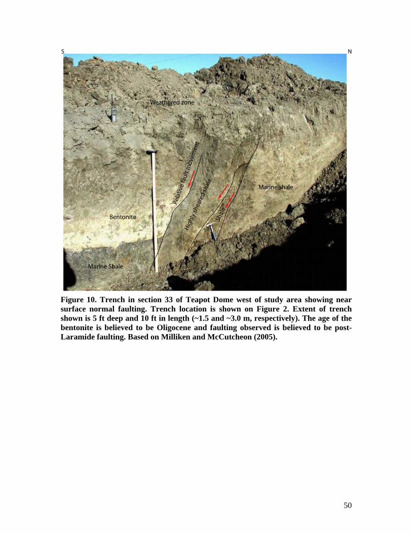
50

Figure 10. Trench in section 33 of Teapot Dome west of study area showing near surface normal faulting. Trench location is shown on Figure 2. Extent of trench shown is 5 ft deep and 10 ft in length (~1.5 and ~3.0 m, respectively). The age of the bentonite is believed to be Oligocene and faulting observed is believed to be post-Laramide faulting. Based on Milliken and McCutcheon (2005).

51

Figure 11A. P-wave filtered shot record with bandpass filter (40-60-120-240 Hz) from the north end of Profile 1. The records show the refracted and reflected arrivals as separate events from each other. A is the direct arrival, B is the refracted arrival and C is the reflected arrival. Scale at the top is the channel number (10 ft (~3.05 m) between channels), while scale on the side is the two-way traveltime.

30.5 m (100 ft)

52

Figure 11B. Filtered P-wave shot record with bandpass filter (40-60-120-240 Hz) from the south end of Profile 1. Refracted and reflected arrivals tend to be merged. Scale at the top is channel number (10 ft (~3.05 m) between channels). A is the direct arrivals and B is the merged reflected and refracted arrivals. Compare with Figure 11a.

30.5 m (100 ft)

53

Figure 12A. P-wave Profile 1 (unmigrated). The shallowest reflection appears at ~140 ms. Reflectivity onset is interpreted to represent the Shannon Sandstone or interfaces just above it. The arrows at the top show the position and name of well logs that were used in mapping faults shown on Figure 7. CMP interval for this other high-resolution P-wave profiles is nominally 5 ft (1.52 m).

54

Figure 12B. P-wave Profile 1 processed as an initial brute stack without refraction statics and with the frequency filter applied before muting of first breaks in the shot domain. Refraction statics corrects for variations in near-surface velocities. Compare with Figure 12a.

55

Figure 13. Unmigrated seismic reflection Profile 1 with interpreted faults. Blue faults were mapped from high-resolution seismic data alone. Pink faults are previously mapped faults cutting the top of the Shannon Sandstone as mapped from well data (Figure 7).

56

Figure 14A. Unmigrated SH-wave seismic profile showing denser faulting (tan colored faults) on Profile 1 than can be observed the P-wave profile. Blue faults correspond with those mapped on the P-wave profile in Figure 13. Pink faults are as in Figure 13. Arrows show location of wells used in mapping faults on Figure 7. CMP interval for this other high-resolution SH-wave profiles is nominally 2.5 ft (0.76 m).

57

3.05 m (10 ft) Figure 14B. Filtered SH-wave shot record with bandpass filter (15-25-40-60 Hz) from the south end of Profile 1. Refracted arrivals and love waves are represented by A and B, respectively. Top mute function is indicated by the red line. Green oval shape shows the position of the reflected arrivals. Numbers across the top are channel numbers.

58

Figure 15A. Unmigrated P-wave reflection profile along Profile 2. This profile shows somewhat more deformation compared to Profile 1. Red faults are previously mapped faults from well data (Figure 7). Blue faults were mapped from the high-resolution P-wave seismic profile.

59

Figure 15B. P-wave reflection along Profile 2 without refraction statics correction processed as an initial brute stack. Compare with Figure 15a.

60

Figure 16. Unmigrated SH-wave seismic profile showing faulting along Profile 2. Red faults are faults mapped from well data (Figure 7). Blue faults correspond with those mapped on P-wave profile in figurer 15a. Tan colored faults are additional possible faults that are not clearly observed on the P-wave profile. This section has been processed with an additional (relative to SH-wave Profile 1) Eigenvector filter (see Jones and Levy (1987) for background information) in order to enhance lateral coherency.

61

305 m (1000 ft)

Figure 17A. An arbitrary seismic profile through the 3D volume matching high-resolution P-wave seismic Profile 1 and continuing to the south (left). A fault within the S2 fault zone (Figure 2) can be drawn through the Frontier (blue marker) and Dakota (red marker) horizons. The fault is projected up to the level of the Shannon interval (about 180 ms). Loss of coherency in the data begins at about 550 ms. The fault line drawn to the level of the Shannon appears in the high-resolution data (Figure 18). Scale at the top shows the line and crossline numbers.

62

Figure 17B. An arbitrary seismic profile through the 3D volume matching high-resolution P-wave seismic Profile 2. The fault, which is interpreted to correspond to the northwesternmost fault (Figure 5A) crossed by Profile 2, is projected up to the level of the Shannon interval (about 180 ms). This fault (red) appears in the shallow subsurface on the P-wave and SH-wave seismic profiles (Figures 15A and 16, respectively).

63

Figure 18. High-resolution P-wave reflection profile, showing the fault (in purple) projected from the arbitrary line extracted from the 3D seismic volume (Figure 17A). This implies that the fault in purple belongs to the S2 fault zone and penetrates from deeper formations through the shallow Shannon interval.

Documents

An Approach to Mapping of Shallow Petroleum Reservoirs