An Animated Guide: An Introduction to Latent Class ... · 1 An Animated Guide: An Introduction to Latent Class Clustering in SAS By Russ Lavery, Contractor ABSTRACT This is the first

1

An Animated Guide: An Introduction to Latent Class Clustering in SASBy Russ Lavery, Contractor

ABSTRACTThis is the first in a planned series of three papers on Latent Class Analysis. Latent Clustering Analysis (LCA) is amethod that uses categorical variables to discover hidden, or latent, groups and is used in market segmentation andmedical research. This paper explores PROC LCA, a free SAS add-in created by The Methodology Center at PennState University. Using this free, and easy to install, add-in allows users of SAS to perform Latent Class Clusteringusing syntax with which they are already familiar.

The managerial output of the Latent Cluster Analysis, (sometimes called Latent Class Analysis) is similar to outputfrom other clustering methods. A researcher/statistician can use PROC LCA to produce a report that, afterinterpretation, contains the following information:

1) The project identified N clusters (and we gave them “cute and interpretable names” – like “Binge Drinker” or“Abstainer”)

2) The clusters have these characteristics (80% of “people in Cluster 1” answered Yes to Question 1)3) The clusters have these relative frequencies (numbers of obs in each of the Clusters we identified”)4) There is x% certainty that a subject belongs in the Cluster to which s/he was assigned.

The above results can be used to create models that can predict, from additional raw data, the likelihood of a newsubject belonging to one of the discovered clusters.

Code and data are included in the appendix of the paper.

INTRODUCTION:PROC LCA can be downloaded for free from the Methodology Center at Penn State University. Installation is veryeasy and the appropriate URL is at the end of the paper.

Comments can be found on the web that assert the superiority of LCA for theoretical reasons. LCA does not assumenormality, homogeneity or a linear relationship and assertions are made that these lack of assumptions make LCAbetter than other methods. My web search investigating the reasons for the superiority of LCA returned many resultssupporting the use of LCA, but a large faction of the supporting entries could be linked to one company – a companythat makes LCA software. The creators of PROC LCA do not make any claim that LCA is superior to other methods.

LCA is used when:1) the data is best collected in frequencies of observations in categories2) the assumptions (we are investigating a process that is categorical and not continuous) match the theory being

investigated3) the results, the identified categorical classes, are easy to communicate to clients.

Use of LCA assumes local independence of variables within clusters and this could be a reason for selecting anothertechnique. LCA assumes that the membership in different latent classes is the only thing that causes observedvariables to be correlated. If you believe that the variables being used in the correlation are related within foundclusters (height and weight might be an example of correlated variables) you might want to use another technique.For pharmaceutical marketers (where TRx and NRx are correlated) might want to consider other methods as well asLCA.

Latent cluster analysis can be used in a variety of business and academic situations. It can be used to discovergroups (e.g. non-drinker, social drinker, binge drinker, addicted drinker … severely depressed, moderatelydepressed, not depressed) from categorical data. This makes LCA a very general tool, especially when theresearcher is willing to “bucket” continuous variables into levels and thereby create discrete variables from continuous(e.g. bucket drinks per week numbers as follows: 0-> never & 1-5->sometimes & 6->15 always or 0-3-> low & 4-7->medium & 8-15-> high). This means this LCA can be applied to almost any data set. PROC LCA can be applied toalmost any sort of cross-tabbed data – even to “found” data from a scholarly articles or found in business reports.

Statistics & AnalysisNESUG 2011

2

The basic process is to:1) “Bucket” continuousvariables into categoricalvariables with two orthree levels.

2) Use PROC LCA tomake a very complexnested frequency table(if we had 6 vars at 3levels we get 243 cells).

3) Use PROC LCA tosolve for 2,3,4,…Ncluster solutions.

4) Determine whichsolution (2-cluster, 3-cluster etc) bestrepresents reality. To theright we see an overallcross-tab of complaintsvs. arrests broken downinto four cross-tabs (with% in each cluster) andthe clustersnamed/interpreted.

Desk OfficersRare Arrest

Occasional Arrest

Regular Arrests

Rare Complaints 388 1 2Occasiona l Complaints 4 0 0Regular Complaints 5 0 0

Homicide DetectivesRare Arre st

Occasional Arrest

Regular Arrests


Vice Squad DetectivesRare Arrest

Occasional Arrest

Regular Arrests


Foot PatrolRare Arre st

Occasional Arrest

Regular Arrests


Overa ll Rare Arrest Occasional Arrest Regular ArrestsRare Complaints 420 88 43Occasiona l Complaints 148 299 164Regular Complaints 73 112 353

Task: recover, from an overall and highly nested cross table,tables for each segment.

An overly simple (just two questions) frequency table.

Recovered latent classes and their frequency tables23% 6%

53%18%

Above data from imaginary “police” research studyFIGURE 1

Figure 1 is an example of a source table, and LCA results, for a police-related example that will be developed later inthe paper. Figure 1 figure shows that PROC LCA was able to take a 2x2 table (the top table) and find a 4 clustersolution that, when summed, approximates the overall cross tab. PROC LCA estimated the answers/characteristicsfor each cluster and the cluster sizes. We see, in Figure 1, that twenty-three percent of the subjects were assigned tothe cluster that was, after analysis of the pattern of answers, named “Desk Officers”. In practice the cross-tabs willinvolve more variables and be more complicated.

5) Create models predicting cluster membership, using variables not used in the segmentation. Statistical techniquesfor categorical Y variables can be used to predict the cluster membership for new observations.

It should be noted that the recovered clusters, or recovered segments, are categorical – but often can be consideredto have some aspects of ordering. This ordering is sometimes raised as a criticism of the use of LCA and is raised bypeople supporting the use of other techniques. As an exploration of this issue we can consider alcohol use habits.There is some ordering in “frequency and quantity of drinking” as one goes from an “abstainer” to an “addicteddrinker”. However a social drinker and a binge drinker might consume the same amount of alcohol per unit monthand the groups might not “separate”, if alcohol consumption per month were plotted on an ordinal scale.

The creators of PROC LCA freely acknowledge that, in many cases, interpretable results come from modeling outputvariables as ordered variables and good results will come from using other techniques. The creators of PROC LCAmake no claim that Latent Cluster Analysis is TRUTH in all cases. However; some research formulations are moreaccurately served, and some theoretical considerations are more closely mapped, by categorical Y and categorical Xvariables. In these cases LCA can be the most appropriate methodology.

CONSTRUCTS OR LATENT VARIABLES:When researchers use the word latent they use it to refer to something that is hidden (un-measurable), or underlying,and which generates observable, measurable characteristics. The factors, in factor analysis, are latent variables.Many path analytic problems focus on latent variables. In fact, most social or business research focuses on latentvariables. A review of the idea of latency would be helpful and is the subject of this section.


3

Figure 2 is a chart thatcould be used to explainthe constructs involved ininvestigating whether“Watching TV Violence”causes “IncreasedAggressiveness”.

“Watching TV violence”and “IncreasedAggressiveness” aretheoretical variables thatcannot be observeddirectly (and so are latentvariables). They can alsobe thought of asgeneralizations orconceptual ideas. Theyare latent variables.Latent variables are oftencalled constructs.

Underlying concepts Constructs or Latent Variables

Watching TV Violence

Increases AggressivenessCauses

RoadRunner

PowerRangers

Wrestling

Itchy &Scratchy

Hitting VerbalAbuse

Threats

Constructs/latent variables can NOT be observed directly.

Constructs/latent variables are observed through multiple measures (multiple operationalisms)The level of the construct determines the level of the observed variables

Constructs/latent variables can be thought of as generalizations.

Er EiEh

Ev

EpEh Et

Unobservable, General

FIGURE 2

Because these two variables cannot be observed, they are said to be latent variables. We assume that theunobservable, latent variables determine the levels of the variables we can see. The variables we can see, like thenumber of hours a child spends watching roadrunner cartoons, are called operationalisms. So we have, in researchmodels, unobservable constructs and observable operationalisms of the latent variables. As a child watches moreTV violence, the number of hours spent watching Road Runner cartoons and Wrestling (etc.) increase.

Constructs are generalizations and investigating generalizations makes research more useful than if the researchwere interpreted using just observable variables. On a policy level, it is more useful to say “watching TV violence”increases “aggressiveness in the nation’s schools” than it is to say “watching roadrunner cartoons makes kids inkindergarten punch each other out”. If one is only thinking in terms of an operational variable, say watchingroadrunner cartoons, the statements one can make are much less interesting and also, potentially, less precise andless generalizable.

If the children who are allowed to watch roadrunner cartoons exhibit greater aggressiveness, one is left wondering ifallowing children to watch cartoons where the background is a desert scene (as in road runner cartoons) increasesaggressiveness. Increased generalizability of results, the ability to use these results in many settings and to makestatements about new and slightly different situations, are important characteristics of research done using the aboveconstruct-operationalism model.

The construct-operationalism way of approaching a research problem is taught through a course called researchmethodology. People trained in social research, or business research, are required to take this course and areexplicitly trained to conceptualize their research projects in this way. People in the hard sciences, like statistics,physics and chemistry, usually do not get a formal exposure to this material. However; I suggest that construct-operationalism is the true model for research - even in the hard sciences.

As an example of construct-operationalism in hard science, consider the following scenario. Imagine some peopleare doing clinical research. They want to tell FDA that their new “active drug” cures some disease in the generalpopulation. “Active drug” is an abstraction/generalization of all of the batches of the “active drug” that were used inthe study. Individual production runs of the test drug can be considered as operationalisms of the construct “activedrug”. The subjects that receive the test drug can be thought of as operationalisms of the construct “patients in thepopulation with the disease”. When we say “the new drug cures a disease”, we want that statement to be interpretedas the drug has the ability to cure cases of the disease in the general population. We do not want to use a researchprocess that only allows us to say: “batch number 32 of the drug cured these seven people”. Even in hard science,we want to generalize results.


4

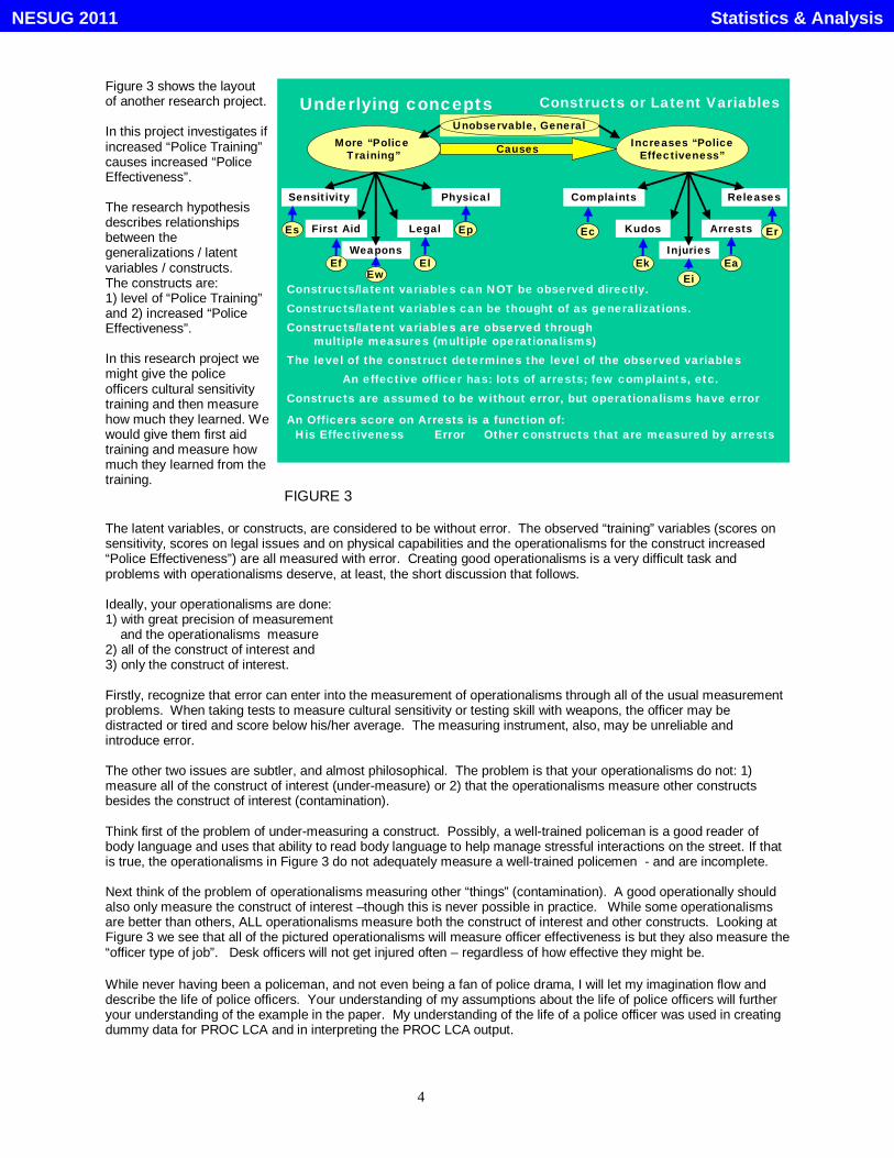
Figure 3 shows the layoutof another research project.

In this project investigates ifincreased “Police Training”causes increased “PoliceEffectiveness”.

The research hypothesisdescribes relationshipsbetween thegeneralizations / latentvariables / constructs.The constructs are:1) level of “Police Training”and 2) increased “PoliceEffectiveness”.

In this research project wemight give the policeofficers cultural sensitivitytraining and then measurehow much they learned. Wewould give them first aidtraining and measure howmuch they learned from thetraining.

Underlying concepts Constructs or Latent Variables

More “Police Training”

Increases “PoliceEffectiveness”Causes

Sensitivity

First Aid

Weapons

Legal

Physical

Arrests

Complaints Releases

Kudos

Injuries

Constructs/latent variables can NOT be observed directly.

Constructs/latent variables are observed through multiple measures (multiple operationalisms)The level of the construct determines the level of the observed variables

Constructs/latent variables can be thought of as generalizations.

An effective officer has: lots of arrests; few complaints, etc.Constructs are assumed to be without error, but operationalisms have error

Es Ep Ec Er

Ef El Ek EaEw Ei

An Officers score on Arrests is a function of:His Effectiveness Error Other constructs that are measured by arrests

Unobservable, General

FIGURE 3

The latent variables, or constructs, are considered to be without error. The observed “training” variables (scores onsensitivity, scores on legal issues and on physical capabilities and the operationalisms for the construct increased“Police Effectiveness”) are all measured with error. Creating good operationalisms is a very difficult task andproblems with operationalisms deserve, at least, the short discussion that follows.

Ideally, your operationalisms are done:1) with great precision of measurement and the operationalisms measure2) all of the construct of interest and3) only the construct of interest.

Firstly, recognize that error can enter into the measurement of operationalisms through all of the usual measurementproblems. When taking tests to measure cultural sensitivity or testing skill with weapons, the officer may bedistracted or tired and score below his/her average. The measuring instrument, also, may be unreliable andintroduce error.

The other two issues are subtler, and almost philosophical. The problem is that your operationalisms do not: 1)measure all of the construct of interest (under-measure) or 2) that the operationalisms measure other constructsbesides the construct of interest (contamination).

Think first of the problem of under-measuring a construct. Possibly, a well-trained policeman is a good reader ofbody language and uses that ability to read body language to help manage stressful interactions on the street. If thatis true, the operationalisms in Figure 3 do not adequately measure a well-trained policemen - and are incomplete.

Next think of the problem of operationalisms measuring other “things” (contamination). A good operationally shouldalso only measure the construct of interest –though this is never possible in practice. While some operationalismsare better than others, ALL operationalisms measure both the construct of interest and other constructs. Looking atFigure 3 we see that all of the pictured operationalisms will measure officer effectiveness is but they also measure the“officer type of job”. Desk officers will not get injured often – regardless of how effective they might be.

While never having been a policeman, and not even being a fan of police drama, I will let my imagination flow anddescribe the life of police officers. Your understanding of my assumptions about the life of police officers will furtheryour understanding of the example in the paper. My understanding of the life of a police officer was used in creatingdummy data for PROC LCA and in interpreting the PROC LCA output.


5

As an overview, I will state that an effective police officer makes lots of arrests and receives letters of praise (kudos –kudos are an archaic word for praise) from the grateful citizens s/he helps. An effective police officer has fewcomplaints, few injuries, and has few arrested subjects released because of paperwork or legal issues. All of theseare generally true.

Let’s think of how an officer’s job affects the measures that we’ve created for police effectiveness.

In my imagination, a desk sergeant has a paperwork job and works inside the police station building. As a result,s/he sees few citizens. He will have few complaints filed, and receive few kudos from citizens. He will have fewinjuries, make a few arrests and have few of his “arrested suspects” released for legal reasons.

A foot patrol officer has a chance to confront violent criminals and meet the public. A good foot patrol officer hasmoderate Complaints, kudos, injuries, and arrests. I assume these officers have about the average number ofarrested suspects released.

Homicide detectives actively work on just a few cases and they routinely talk to very upset and easily offend people.Homicide detectives have moderate complaints, kudos, injuries, and low arrests. I assume, since everyone strugglesso intensely to be released from a homicide charge, that they have a lot of their “perps” released after arrest.

People on the vice squad can make lots of arrests (because in many large cities it’s easy to pull someone off a streetcorner and arrest them) but this kind of officer gets lots of complaints. In my imaginary police world, vice suspectsoften file complaints against the officers as a way of letting off their aggravation at being arrested and also as a formof revenge (by making the officers spend time at his desk filling out forms in response to the complaint). A vice squadofficer has high complaints, low kudos, low injuries, and high arrests. I assume these officers have about the averagenumber of arrested suspects released.

With the above story in mind, you can easily see how our operationalisms for effective policing also measure theconstruct “officer type of job”. To make the situation worse, the operationalisms measure other constructs as well. Inthe real world, operationalisms always measure more than one construct and are always contaminated. Goodoperationalisms have less “contamination” than poor operationalisms. As you can imagine, researchers can havelots of discussions over operationalism issues.

As an aside, it is never safe to operationalize a construct with just one variable. Additionally, self-reported variablesare notoriously unreliable. Constructs should be measured by several different variables and using variables ofdifferent types. Good research practice requires a researcher should use a mixture of self-report, historical records,direct observation by the research team members, and even physical measurements to capture a construct.

More detail about our data follows:

A program, in the abstract of the paper, will allow you to reproduce the results shown below. Changing parameters inthe part of the SAS program that generates dummy data will allow you to experiment with how well PROC LCA canfind TRUTH - in whatever messy data set you create.

I will spend a little time describing the parameters that I used to create the data used in this analysis. The parametersare used to create dummy data against which I ran PROC LCA. I think generating dummy data is an effectivelearning technique. The learning process is to create dummy data with known characteristics and then see how wellthe technique being used can recover the known characteristics designed into the data.

Please see Figure 4 for our model and the parameters. PROC LCA assumes ONLY ONE latent variable (unlike factoranalysis). LCA assumes that categorical classes in the latent variable cause the values we observe in theoperationalisms. It also assumes the errors in the operationalisms are uncorrelated.

In my imaginary research project I reviewed six months of information on arrests, complaints, prisoners released forsome problem with paperwork or the legality of the arrest, injuries to the police officer, and kudos. Kudos is anarchaic word for praise, and I needed a word that did not start with P because I’d used a variable beginning with p ina previous slide. On the slide below you can see the average counts in six months for each of these variables and byofficer type. I used base SAS, and a loop, to generate hundreds of observations with these characteristics. I alsoadded an error term to each variable for each observation so the officers in a cluster did not have identicalcharacteristics. Feel free to change these parameters to play with the model and PROC LCA.


6

The variables started outas being continuous and Iused PROC Rank to groupthem into three categoriesthat I labeled: rare,occasional and regular.

In the SAS program in theappendix, there areseveral sections thatproduce cross tabs ofvariables. These crosstabs are not required for aresearch project but isuseful to investigate howthe magnitude of thedesigned in error term hasaffected the observedresults.

Please look back at Figure1 and notice that two deskofficers made regulararrests. This is the resultof the error parameter inthe program introducingerror to the measuredvariable.

We are examining records on Police officers

What is the IMAGINARY backstory for this example.

One record per officer: variables to right.Increases “Police

Effectiveness”

Arrests

Complaints Releases

Kudos

InjuriesEc Er

Ek EaEi

Job Assignment:Desk, Foot, Vice

Homicide

Arrests

Complaints Releases

Kudos

Injuries

Four Kinds of officer: to right.

Backstory (average counts in 6 months):Vice: 20 Arrests 10 Complaints

2 Releases 2 Injuries 2 Kudos

Foot: 5 Arrests 5 Complaints 2 Releases 5 Injuries 5 Kudos

Desk: .1 Arrests .5 Complaints 1 Releases .1 Injuries .1 Kudos

Homicide: 1 Arrests 5 Complaints 2 Releases 2 Injuries 2 Kudos

Use Proc Rank to assign to 3 categories:1) Rare2) Occasional3) Regular

300Officers

900Officers

400Officers

100Officers

FIGURE 4If you want to play with the program, and create a custom data set, look in the SAS program in the appendix for thelines below/*TrueSegments: the names of the classes/segments. In a research project, this will not be known *//*ClassPrev :number of respondents in each class. In a research project, this will not be known *//*ComplntsAvg :average number of complaints for the class in 6 months - from police records *//*KudosAvg :average number of complimentary letters for the class in 6 months - from police records*//*InjuryAvg :average number of injuries for the class in 6 months - from police records*//*ArrestAvg :average number of arrests made for the class in 6 months - from police records*//*Releasing :average number of suspects released for PROCedural reasons for the class in 6 months - from police records*/%let TrueSegments = Desk Foot Hom Vice ; /*Name of segments*/%let SgmntCount = 400 900 100 300 ; /*officers/segment*/%let ComplntsAvg = .5 5 5 10 ; /*avg compaints/segment*/%let KudosAvg = .1 5 2 2 ; /*avg Kudos/segment*/%let InjuryAvg = .1 5 2 2 ; /*avg Injuries/segment*/%let ArrestAvg = .1 5 1 20 ; /*avg arrests/segment*/%let ReleaseAvg = .1 2 2 2 ; /*avg released/segment*/You can change the parameters to produce new datasets and see how well PROC LCA performs against your newdata.

ISSUES WITH LATENT CLUSTER ANALYSIS

Latent cluster analysis can have algorithmic problems with local minimum and maximum. It is a good idea to makeseveral runs of PROC LCA using several different “starting points” to assure that the output is stable. If the outputfrom your several runs is unstable, the creators of PROC LCA suggest you create a loop to runs several hundredLCAs with different starting points. The creators of PROC LCA suggest you compile the output of the hundred LCAruns and see where the modal points for output parameters might be and they describe this process in their book.


7

Missing values are often present in data and do not cause PROC LCA undue problems. It is assumed that missingvalues are missing completely at random and if this is not the case, additional effort and thought must be allocated tothe data itself.

LCA assumes that, after a valid solution is found, variables are uncorrelated within clusters and this might not be thecase.

PROC LCA output isharder to read than theexamples in the book thatwas written by theauthors of PROC LCA.The book format is usedin Figure 5.

I should warn the readerthat Figure 5 shows newdata – data not collectedwith the police example. Iapologize for using a newdata set but it was verydifficult to construct onedata set that wasinteresting enough, smallenough and well behavedenough to allow it to beused to illustrate all of thepoints in this paper. Iprefer to stick with onedata set through a wholepaper. It just was notpossible.

0.0007130.000713 0.020188 0.009025 ------> 0.02381

0.0201880.000713 0.020188 0.009025 ------> 0.674603

0.0090250.000713 0.020188 0.009025 ------> 0.301587

-----------sum 1

Found Classes-> PBS_Watcher ESPN_Low ESPN_MegaMembership Prob .30 .50 .20

Follows Y .05 .85 .95 Soccer N .95 .15 .05

Follows Y .05 .05 .95 Football N .95 .95 .05

Follows Y .05 .05 .95 Baseball N .95 .95 .05

.3*( .05 * .05 * .95) + .5*( .85 * .05 * .95) + .2*( .95 * .95 * .05)

.3*( .05 * .05 * .95)

Prob of being in classesgiven measurements: Y N N

Only 67% chance of a Y N Nbeing from Class 2

Has

characteristicsof

good

Solution

Precision of assignment 67-76

FIGURE 5

In Figure 5 you see the results from PROC LCA in an easy-to-read format. In the grayish box in the bottom of theslide you see the results from running a PROC LCA on a new and imaginary data set. What you don’t get fromPROC LCA, are names of the “Found Classes” (e.g. “PBS_Watcher”). The “Found Classes” are the results of theresearcher interpreting data and matching patterns on the PROC LCA output with his/her understanding of reality.

We see, in Figure 5, that the researcher is interpreting a three LCA solution. The membership probabilities, or therelative size of the groups, are 30%, 50% and 20%. The researcher had asked three questions.

The questions are:Do you follow soccer?Do you follow football?Do you follow baseball?

The answers were a categorical yes or no.

We assume that the researcher has also run a two-cluster LCA, a three cluster LCA, a four-cluster LCA, and likelyeven a five-cluster LCA. Figure 5 only shows the results the three-cluster LCA and also how the researcher hasmapped the numbers in the output listing to his understanding of external reality. What we see, in the output listing,are the percentage of people in the three-cluster solution that have answered a certain way. In cluster one, fewpeople follow any of the sports. In cluster two (named ESPN_low) the people follow soccer. Maybe this cluster ismade up of young people who played soccer in school or people exposed to soccer outside of the US. Members ofthe third cluster seem to follow all sports. 95% of the people in the third cluster (ESPN_mega) said yes to all of thethree questions.

Figure 5 has the characteristics of a good solution – at least after a first level of examination. The sizes of theclusters and the pattern of responses to the questions map well to our understanding of the external reality. Thepatterns are distinct and interpretable. The sizes of the segments are “reasonable”.

The second level of examination is to investigate the stability of assignments. This is done over each pattern ofresponses and, with three two-level responses, there are eight possible patterns of yes and no responses. One testfor stability is shown in the formula at the top of the Figure 5. In this formula, we are investigating the chance ofresponding yes, no, and no to the three questions ….. given that you are from a particular class.


8

You can see, the probability we are calculating is: the percent of the total number of subjects in a “Found Class” timesthe probability of a yes on question one times the probability of a yes on question two times the probability of a yes onquestion three ….then that whole thing divided by… that same calculation done for all groups.

We see is that the most common response pattern in the group we’ve named ESPN_low (the response pattern YNN)only has a 67% chance of coming from somebody in ESPN_low. Almost 2/3 of the subjects with this responsepattern were assigned to other clusters. This should decrease our faith in this solution.

Checking, of each response pattern probability and also each subject’s classification probability (in anothercalculation that was not shown) is essential if these “found classes” are to be used as dependent variables in a latersteps in a modeling process. Said in another way, good practice requires checking two (question pattern andsubject) types of classification probability if a researcher wants to use cluster assignments as Y variables in furthermodeling,

Inside a particularsolution the stability ofassignment can varygreatly among classes.

In the figure to the rightyou can see that theprobability of a responsepattern YYY is verystrongly associated withthe group we’ve namedESPN_mega.

A high (.99) likelihood ofassignment is acharacteristic of a goodsolution.

Let’s discuss some morecharacteristics of a goodsolution.

Unfortunately, to do this Iwill bring in yet anothernew data set

Found Class PBS_Watcher ESPN_Low ESPN_MegaMembership Prob .30 .50 .20

Follows Y .05 .85 .95 Soccer N .95 .15 .05

Follows Y .05 .05 .95 Football N .95 .95 .05

Follows Y .05 .05 .95 Baseball N .95 .95 .05

.3*( .05 * .05 * .05) + .5*( .85 * .05 * . 05) + .2*( .95 * .95 * .95).2*( .95 * .95 * .95)

Prob of being in classesgiven measurements: Y Y Y

0.00003750.0000375 0.001063 0.171475 --> 0.000217

0.0010630.0000375 0.001063 0.171475 --> 0.006157

0.1714750.0000375 0.001063 0.171475 --> 0.993626

--------------Sum 1

99% chance of a Y Y Y beingfrom Class 3

Has

characteristicsof

good

Solution

Precision of assignment 67-76

FIGURE 6


9

Figure 7 uses a new dataset to illustrate facilitatediscussion of how goodquestions exhibitdependence across“Found Classes”.

For question one, all“found classes” had thesame responseProbability. Thisquestion does not help usfind a solution. Theory,or our understanding ofreality, should havedirected us away fromasking this question.

The third and fourthquestions have greatdifferences in theirresponse patterns acrossthe “Found Classes”.These questions will beof use to the researcher.

Criteria 1: distribution varies across classes 50Independence: Knowing something about X does not tell you anything about Y.

If the prob. of a level of response is the same acrossall classes, the variable is not of much use in themodel or the number of classes is incorrect.

Found Class Non_drinker Social Addict Binge

Drank Beer Y .99 .99 .99 .99 in last year N .01 .01 .01 .01

Drank Y .02 .30 .95 .50 this week N .98 .70 .05 .50

5 drinks-1 day Y .01 .02 .50 .95 in last year N .99 .98 .50 .05

Drank Alone Y .01 .05 .95 .25 in last year N .99 .95 .02 .75

Was Sick Y .01 .03 .50 .80 while drinking N .99 .97 .50 .20 in last year

INDEPENDENT and of little use

DEPENDENT and of use

FIGURE 7

Figure 8 illustratesanother characteristic ofgood questions. Theyhave responses witheither high or lowprobabilities.

This part of the analysisis very parallel to factoranalysis, wherequestions with high factorloadings help identify thefactors.

The nondrinkers are verydifferent in their patternsfrom other people.Additionally, becausethey’re probabilities areclose to zero and one wecan consider this to be ahomogeneous group – areal group that likelyexists in the populationas a whole.


Drank Beer Y .99 .99 .99 .99 in last year N .01 .01 .01 .01




Was Sick Y .01 .03 .50 .80 while drinking N .99 .97 .50 .20 in last year

Criteria 2: Item-response probs are close to 1 or 0High or low probabilities are associated with goodsolutions.





HeterogeneousHomogeneous

Real Group ?Real Group !

If the prob. of a level of response is the same acrossall classes, the variable is not of much use in themodel or the number of classes is incorrect.

FIGURE 8


10

The “Found Class” that was named “social drinkers” is much less homogeneous than the “non-drinker” “FoundClass”. The fact that their response percentages are not close to zero and one could be caused by a naturalheterogeneity in a group both truly exists and that is truly heterogeneous. It could also be caused by this being a poorsolution. It could be that the “Found Class” named “social drinker” is not one true class. It could be that that thisgroup is a mixture of two homogeneous groups resulting in the heterogeneous group we see in Figure 8. It could bethat the “Found Class” named “Social Drinker”, when we ask PROC LCA for a five group solution, separates into twogroups who have their probabilities close to zero and one.

MEASURES OF HOMOGENEITY AND SEPARATION:

Because of the individual differences in classification error people often look at the classification probabilities over allthe subjects using a formula that has the name of “Entropy”. The formula is:

E = 1 - _________________________________

N log C

Σ -pic log picΣi=1

n

C=1

C

MEASURES OF GOODNESS OF FIT:

LCA has a few measuresof goodness of fit andthey are all based on astatistic called G2.

Unfortunately, to havethe example fit easily ona slide I must introducestill another new data set.

This new data set onlyhas two questions andyou can see the nestedfrequency table on theleft-hand side of Figure 9.

PROC LCA looks at theobserved nestedfrequency table and triesto create a nestedfrequency table thatclosely approximates thetable created from thedata.

C -1

Does a Recovered Latent Class Model make a closeapproximation of the observed data?

Ho is that the model is a good fit and we hope not to reject it?

Absolute model fit is measured bythe Likelihood Ratio Statistic G2

„ƒƒƒƒƒƒƒƒƒƒƒƒƒƒƒƒƒƒƒƒƒƒƒƒƒ…ƒƒƒƒƒƒƒƒƒƒƒƒ†‚Numbers from raw data ‚ Number of ‚‚ ‚ Subjects ‚‡ƒƒƒƒƒƒƒƒƒƒƒƒ…ƒƒƒƒƒƒƒƒƒƒƒƒˆƒƒƒƒƒƒƒƒƒƒƒƒ‰‚Q1Answer ‚Q2Answer ‚ ‚‡ƒƒƒƒƒƒƒƒƒƒƒƒˆƒƒƒƒƒƒƒƒƒƒƒƒ‰ ‚‚1 yes ‚1 yes ‚ 30.00‚‚ ‡ƒƒƒƒƒƒƒƒƒƒƒƒˆƒƒƒƒƒƒƒƒƒƒƒƒ‰‚ ‚2 no ‚ 37.00‚‡ƒƒƒƒƒƒƒƒƒƒƒƒˆƒƒƒƒƒƒƒƒƒƒƒƒˆƒƒƒƒƒƒƒƒƒƒƒƒ‰‚2 no ‚1 yes ‚ 28.00‚‚ ‡ƒƒƒƒƒƒƒƒƒƒƒƒˆƒƒƒƒƒƒƒƒƒƒƒƒ‰‚ ‚2 no ‚ 155.00‚‡ƒƒƒƒƒƒƒƒƒƒƒƒ‹ƒƒƒƒƒƒƒƒƒƒƒƒˆƒƒƒƒƒƒƒƒƒƒƒƒ‰‚All ‚ 250.00‚Šƒƒƒƒƒƒƒƒƒƒƒƒƒƒƒƒƒƒƒƒƒƒƒƒƒ‹ƒƒƒƒƒƒƒƒƒƒƒƒŒ

========================Fit statistics:========================Log-likelihood: -269.70G-squared: 0.01AIC: 10.01BIC: 27.62CAIC: 32.62Adjusted BIC: 11.77Entropy R-sqd.: 0.44Degrees of freedom: -2

G2 = 2 f w logw=1

W

( )f w ^

f w

Problem if you have missing dataCompare G-squared to Chi-Squared

Problem if youhave Sparse data.We want N/W >5.

W=#of cells in Xtab = 4

Absolute Model Fit page 81-93

DofF = W - P -1

P =

+

C (Sum of (levels -1))

C=#ofClasses = 2

DofF = 4 - ( 1 + 2 (1+1)) -1Q1Answer has 2 levelsQ2Answer has 2 levels

FIGURE 9

I pasted the fit statistics from the PROC LCA into the slide in Figure 9. The PROC tells us that G2 is .01. G2 is thencompared to a chi-squared and the degrees of freedom for G2 is the messy calculation shown in Figure 9. LCA doesthis calculation for us, but let us duplicate its work as a bit of practice.

The degrees of freedom calculation is W - P –1. Calculating W is easy but calculating P takes several steps.W is the number of cells in the crosstab and here it is four. P is the result of a sub-calculation.

To calculate P, we start from the most nested question (Q2 is shown nested within Q1) and as we work “outwards”,we do the following: For each question we take a look at the number of levels of that question and subtract one. (here we see Q1: 2-1=1 and Q2: 2-1=1 )We sum up the result of that subtraction over all the questions. 1+1

We multiply that sum by the number of Found Classes. We had asked PROC LCA for a two-class solution. 2*(1+1)


11

We add the result of this multiplication to a number we calculate by subtracting one from the number of classesrequested from PROC LCA and we have P. Thankfully, PROC LCA does this calculation for us.

The calculation of G2 itself is more complicated. The formula basically compares the frequency found in a cell (fw)with the expected value of fW-hat calculated by PROC LCA. If the numbers are close, then we have a good fit, so asmall value of G2 indicates a good model. We assume that the model is good and reject the model when G2 getslarge.

We are going to construct, from response probabilities predicted by LCA, the probability table from the raw data thatcan be seen in Figure 10

Figure 10 shows more ofthe calculations. Notethat the words class andgroup are usedinterchangeably.

The white box in the topleft shows output fromPROC LCA. Theprobabilities of being inthe two classes are:.3478 and .6522.

I know, because Idummied up the data,that there are 250observations in the dataset. That lets us predictthe number of people ineach class to be: 86.95and 163.05 (250 *.6522).

For Class 1 theprobability of a Yes-Yesis .6402 * .5468

Class1 n Classn N86.95 163.05 250

Obs . Cell Calculated Q1 Q2 Predic tedCount n P ercent P ercent N-for cell

C las s 1 Q1= 1 Y Q2= 1 Y 30 86.95 0.6042 0.5468 28.72624189Q2= 2 N 37 86.95 0.6042 0.4532 23.80894811

Q1= 2 N Q2= 1 Y 28 86.95 0.3958 0.5468 18.81801811Q2= 2 N 155 86.95 0.3958 0.4532 15.59679189

C las s 2 Q1= 1 Y Q2= 1 Y 30 163.05 0.0882 0.0637 0.916070337Q2= 2 N 37 163.05 0.0882 0.9363 13.46493966

Q1= 2 N Q2= 1 Y 28 163.05 0.9118 0.0637 9.470214663Q2= 2 N 155 163.05 0.9118 0.9363 139.1987753

Total 250

G2 = 2 f w logw=1

W

( )f w ^

f wClass: 1 2% of N in class 0.3478 0.6522

N (# of obs) X 250 X 250(pred)n in class 86.95 163.05

Class: 1 2 0.3478 0.6522Rho estimates(item response probs):Response category 1: yesClass: 1 2 Q1Answer : 0.6042 0.0882 Q2Answer : 0.5468 0.0637Response category 2: noClass: 1 2 Q1Answer : 0.3958 0.9118 Q2Answer : 0.4532 0.9363

Fit statistics:G-squared: 0.01

Absolute Model Fit page81-93

FIGURE 10

PROC LCA thinks that there are 86.95 people in Class 1 and, for Class 1, the probability of a Yes-Yes is.6402 * .5468. So we expect class 1 to contribute 28.72 (86.95 * .6402 * .5468.) “counts” to the Yes-Yescell in the cross-tab PROC LCA created from the original data.

PROC LCA thinks that there are 163.05 people in Class 2 and, for Class 2, the probability of a Yes-Yes is.0882 * .0637. So we expect Class 2 to contribute .916 (163.05 *.0882 * .0637) “counts” to the Yes-Yescell in the cross-tab that PROC LCA created from the original data. The expected number of subjectsresponding Yes-Yes is: 28.72 + .916 = 29.64 You can look at Figure 9 to see the table from the rawdata had a count of 30.0. The fit is close for this cell.

PROC LCA thinks that there are 86.95 people in Class 1 and, for Class 1, the probability of a No-Yes is.3958 * .5468. So we expect class 1 to contribute 18.82 “counts” to the No-Yes cell in the cross-tabPROC LCA created from the original data.

PROC LCA thinks that there are 163.05 people in Class 2 and, for Class 2, the probability of a No-Yes is.0882 * .0637. So we expect Class 2 to contribute 9.47 “counts” to the Yes-Yes cell in the cross-tab thatPROC LCA created from the original data. The expected number of subjects responding No-Yes is: 18.82+ 9.47 = 28.29 and you can look at Figure 9 to see the table from the raw data had a count of 28.0.

We see that calculated counts are fitting the data pretty well and we should expect that our test statisticsto be small.


12

Figure 11 shows the endof the calculations.

Here, for each of the 4cells, we calculated thepredicted cell count.

The far right column inFigure 11 shows thecontribution for each cellto the total G2.

Unfortunately the formulacan not be shown insidethe cells in thisPowerPoint but theformula is repeated in thetop right-hand corner ofFigure 11 and the resultis in the bottom right-hand corner. We havereproduced the G2

statistic (.009533 ~= .01).

Answer Obs. Group 1 Group 2 Group 1 & 2 Result ofCombination Count Pred n Pred n Cell total FormulaFor Cell For Cell For Cell For Cell For Cell For CellQ1=1 Q2=1 30 28.72624 0.91607 29.6423122 0.719674

Q2=2 37 23.80895 13.46494 37.2738878 -0.54576

Q1=2 Q2=1 28 18.81802 9.470215 28.2882328 -0.57352Q2=2 155 15.59679 139.1988 154.795567 0.409135

Total 0.009533

G2 = 2 f w logw=1

W

( )f w ^

f wClass: 1 2% of N in class 0.3478 0.6522

N (# of obs) X 250 X 250(pred)n in class 86.95 163.05

Class: 1 2 0.3478 0.6522Rho estimates(item response probs):Response category 1: yesClass: 1 2 Q1Answer : 0.6042 0.0882 Q2Answer : 0.5468 0.0637Response category 2: noClass: 1 2 Q1Answer : 0.3958 0.9118 Q2Answer : 0.4532 0.9363



Absolute Model Fit page81-93

FIGURE 11

The G2 statistic is anabsolute measure ofabsolute model fit.

Our usual process is totry to create a model thatexplains well and that isparsimonious (fewclusters and fewparameters to estimate).

To do this, we also needrelative measures of fitthat will allow us tocompare different modelsas we strive forparsimony.

There are twoapproaches to evaluatinga parsimonious model.

They are: 1) thelikelihood ratio test of G2

and 2) comparinginformation criteria.

Do the added “restrictions” cause a significant drop in G2

Relative Model Fit page86You can test relative model fit as you develop a moreparsimonious mode.Two Approaches:

Likelihood ratio test of G2

Compare Information Criteria

Likelihood ratio test of G2

Models must be nestedThe more parsimonious model has more parameter“restrictions”

G2 change = G2 restricted - G2 full

DofF change = DofF restricted - DofF full

Do repeated analysis and PlotG2, AIC and BIC as a function ofthe number of classesrecovered.

Compare Information CriteriaAIC = G2 + 2P and BIC = G2 + [ln (N)]PSmaller is better

FIGURE 12

AIC and BIC penalize more complex models and the values for AIC and BIC can be seen in Figure 9.

Results below are from the Police Example: The code included in appendix.


13

Please refer back toFigures 3 & 4 forinformation about thepolice example.

In the example, I createda dummy data set with 4different types of policeofficer.

Imagine I checked officerrecords as to the numberof: complaints, kudos,injuries, arrests, andprisoners later released.

In the program, I loopedto create an observationfor each officer, addederror, and bucketed thenumbers (“rarely”,“occasionally” and“regularly”).

Worked example with code 81-94

0200400600800

100012001400160018002000

2 3 4 5 6

G-squared:AIC:BIC:

# of Clusters 2 3 4 5 6Recovered Clusters Clusters Clusters Clusters ClustersG-squared: 129.46 150.74 161.5 306.46 1566.23AIC: 259.46 258.74 247.5 370.46 1608.23BIC: 612.96 552.41 481.35 544.49 1722.43

FIGURE 13

As I started the example, I looked at the raw frequencies and saw variability on the data set level. This gave somehope that patterns of responses might exist in the 5-variable cross-tab that PROC LCA would create. If there is novariability in the data set, all responses are uniform and there is one pattern of responses (one cluster). If there isvariability in the data set, there might be clusters that are uniform in their responses or there might be one custer ofpeople with a lot of variability within the cluster.

I instructed PROC LCA to run analyses for two clusters up to six clusters. The fit statistics, in Figure 13, suggest thattwo, three or four clusters might be reasonable solutions. I looked at the PROC LCA output for three and fourclusters and was most comfortable interpreting the four-cluster solution against my understanding of reality. Outputfrom the four-cluster solution is included below (Figures 14 to 16).

I added some text boxes of information onto the figures so that we wouldn’t have to remember as much about theproblem. While questions are hidden by my added boxes of typing/information, the questions are in the order inwhich we always have presented them and can be discovered by looking back in the paper.

Remember we had three levels of response, created by the use of PROC Rank. We assigned people to “rarely”,“occasionally” and “regularly” (coded rare, occasional and regular to save space).

Unfortunately, the output from PROC LCA is grouped by level of response over all questions. This is different fromthe format used in the Proc LCA book and what I have used in previous slides. This way Proc LCA presents results isawkward, at least for me, to interpret and I have avoided it until now.

Using the format from PROC LCA:First, we will first see an analysis of the lowest response level (“RARE”) in Figure 14.Then we will then see an analysis of the middle response level (“OCCASIONAL”) in Figure 15.Then we will then see an analysis of the highest response level (“REGULAR”) in Figure 16.

As mentioned before, the format of the output in the book is easier to use than the output from PROC LCA (shownbelow).


14

RARE: First, look at thesizes of the clusters.

PROC LCA gives us thepercentage of the originaldata that was assigned toa particular cluster. Thereturned percentagesclosely match what weknow about theenvironment. What wecalled Homicide is thesmallest class.

76.18% of the homicideofficers “Rarely getkudos”. 74% “Rarely areinjured”. 99% “Rarelymake arrests”. Theseare characteristics ofpeople who work on afew cases and who donot interact with thegeneral public.

99.23% of the deskofficers “rarely make anarrest”.

Parameter Estimates

Class membership probabilities: Gamma estimates (standard errors)Class: 1 2 3 4 0.1767 0.2409 0.0500 0.5323 (0.0100) (0.0111) (0.0075) (0.0123)

Item response probabilities: Rho estimates (standard errors)

Response category 1: Rare

Class: 1 2 3 4 GrpComplaint: 0.0004 0.9791 0.0097 0.1647 (0.0013) (0.0160) (0.0328) (0.0124)

GrpKudos : 0.7326 0.9631 0.7618 0.0016 (0.0269) (0.0096) (0.0520) (0.0016)

GrpInjuries : 0.6887 0.9722 0.7438 0.0015 (0.0279) (0.0083) (0.0531) (0.0015)

GrpArrests : 0.0059 0.9923 0.9970 0.1634 (0.0190) (0.0043) (0.0079) (0.0124)

GrpReleases : 0.1386 0.8694 0.1466 0.1854 (0.0203) (0.0175) (0.0655) (0.0130)

Vice 300 Foot 900Desk 400 Hom 100

%let TrueSegments =Desk Foot Hom Vice;%let SgmntCount = 400 900 100 300 ;%let ComplntsAvg = .5 5 5 10 ;%let KudosAvg = .1 5 2 2 ;%let InjuryAvg = .1 5 2 2 ;%let ArrestAvg = .1 5 1 20 ;%let ReleaseAvg = .1 2 2 2 ;

FIGURE 14

OCCASIONAL: InFigure 15 we see thepercentages of subjectsclassified as“Occasional”.

65.66% of the homicidedetectives occasionallyget complaints.

.26% of the officers in thegroup that we havenamed "Desk Officers",make occasional arrests.

.09% of the officers in thegroup that we havenamed homicide makeoccasional arrests.

55.02% of the officers inthe group that we havenamed foot, makeoccasional arrests.

Parameter Estimates



Response category 2: Occasional


GrpKudos : 0.2042 0.0318 0.2209 0.1180 (0.0238) (0.0088) (0.0496) (0.0109)

GrpInjuries : 0.2534 0.0204 0.2144 0.1473 (0.0260) (0.0071) (0.0488) (0.0121)

GrpArrests : 0.0003 0.0026 0.0009 0.5502 (0.0010) (0.0025) (0.0034) (0.0167)

GrpReleases : 0.5439 0.0935 0.6146 0.5570 (0.0292) (0.0151) (0.0659) (0.0166)

Vice 300 Foot 900Hom 100


Desk 400

FIGURE 15


15

REGULARLY: Finally,look at the patternswhere the classification isregularly or high.

99.91% of the vice squadofficers make a highnumber of arrests. Theyalso have 31.75 % of theofficers classified as“high % for suspects laterreleased”. The .9991 onthe GrpComplaint rowtells us that almost allvice squad officers areclassified as getting“regular” complaints.

The recovered sizes ofthe four groups and thecharacteristics of thegroups agree with theparameters that wereused in creating thedummy data for PROCLCA.

Parameter Estimates



Response category 3: Regular / High


GrpKudos : 0.0631 0.0051 0.0173 0.8804 (0.0164) (0.0037) (0.0187) (0.0110)

GrpInjuries : 0.0578 0.0074 0.0418 0.8512 (0.0146) (0.0044) (0.0256) (0.0122)

GrpArrests : 0.9938 0.0051 0.0021 0.2864 (0.0190) (0.0035) (0.0072) (0.0153)

GrpReleases : 0.3175 0.0371 0.2388 0.2576 (0.0273) (0.0095) (0.0501) (0.0146)

Vice 300 Foot 900Hom 100


Desk 400

FIGURE 16

The managerial output from PROC LCA is similar to the output from other clustering methods. You getcharacteristics of the clusters that an analyst can use, by comparing the output to his/her understanding of theenvironment. The managerial output is clusters with useful name, sizes of the clusters and estimates of classificationaccuracy.

SUMMARY:PROC LCA is a free add-in to SAS that you can download from the Methodology Center at Penn State University. Itis easy to install and use. The authors of the program have also written a very readable companion book: “LatentClass and Latent Transition Analysis: With Applications in the Social, Behavioral, and Health Sciences”.

We saw in the paper above that PROC LCA was very successful in recovering, from a dummy data set, the structurethat was designed into the data set - even after error was added to the data.

There is discussion among researchers as to the superiority of LCA over traditional clustering methods. Regardlessof the position one takes on this issue, LCA is good to have this tool on your tool-belt.

The code for the example used in this paper is included in the appendix.

A summary of the steps in a PROC LCA analysis1) Review the literature and talk with your subject matter expert. While there are statistics and programming skills

needed in a Latent Cluster Analysis, interpreting the results requires knowledge of the underlying issues.2) Check out the overall univariate frequencies. If there is little variability in the overall frequencies, there isn’t much

of a hint that these variables will support a successful investigation. If the variables have three levels, and themarginal levels are all .33, you might be able to find interesting segments but the data does not suggest that. Ifthe variables have three levels, and the marginal levels are .1 .4 and .6, there is some evidence that peopleinside the large sample are not replying uniformly and it gives stronger hope for the idea that there are patternsof responses inn the data that are coming out of different latent classes.

3) Consider creating a validation holdout sample, or even two holdouts (improvement and validation). As in anymodel results are biased towards the sample on which the model was developed. It is good practice to holdsome percentage of your original data out of the modeling process and use that holdout to see if the modelgeneralizes to new data.

4) Run PROC LCA and ask PROC LCA for solutions involving different numbers of latent classes. Run PROC LCAwith different starting points to investigate the existence of local minimums/maximums.

5) Plot the goodness of fit measures for each of the N latent class solutions that you ask PROC LCA to produce.This should give hints as to the true number of latent classes in the data.


16

6) Investigate the stability of the assignment by investigating stability for each response pattern and of eachsubject’s assignment.

7) Focusing on the classes suggested by step five, you should compare the results from the analysis to yourunderstanding of the world (or the little part of it you are researching) and see which solution is mostinterpretable and most likely to be valid.

REFERENCES:

Thanks to the group that created the free PROC LCA program :The Methodology Center http://methodology.psu.edu/index.phpThe Methodology Center is an interdisciplinary center that comprises faculty, research associates, post-docs, andstudents from several academic disciplines, including human development, psychology, statistics, and public health.Their work is funded by the National Institutes of Health and by the National Science Foundation.

Linda M. Collins, Ph.D. &Director, The Methodology CenterThe Methodology CenterThe Pennsylvania State University 204 E. Calder Way, Suite 400 State College, PA 16801

Collins & Lanza “Latent Class and Latent Transition Analysis: With Applications in the Social, Behavioral, and HealthSciences” (2010) Wiley Book web site is: http://methodology.psu.edu/latentclassbook/

Magidson & Vermunt “Latent class models for clustering: A comparison with K-means” , Canadian Journal ofMarketing Research, Volume 20, 2002 http:www.statisticalinnovations.com

Magidson, J. A. “Latent Class (Finite Mixture) Segments: How to find them and what to do with them.(2010)” Presented at 2010 Sensometrics Meeting: Rotterdam, The Netherlandshttp://www.statisticalinnovations.com/articles/Magidson.Sensometrics2010.pdfin

Thompson, David M. “ Performing Latent Class Analysis Using the CATMOD PROCedure” Proceeding of the SASuser group International (31) http://www2.sas.com/PROCeedings/sugi31/201-31.pdf

CONTACT INFORMATIONYour comments and questions are valued and encouraged. Contact the author at:

Russ Lavery Bryn Mawr, PA Email: [email protected] Web page for all papers: Russ lavery.com

SAS and all other SAS Institute Inc. product or service names are registered trademarks or trademarks of SASInstitute Inc. in the USA and other countries. ® indicates USA registration.Other brand and product names aretrademarks of their respective companies.


Documents

An Animated Guide: An Introduction to Latent Class ... · 1 An Animated Guide: An Introduction to Latent Class Clustering in SAS By Russ Lavery, Contractor ABSTRACT This is the first