An Anatomy of Credit Booms: Evidence from Macro Aggregates and Firm Level Data

Enrique G. Mendoza (University of Maryland)

and Marco E. Terrones (IMF) Paper presented at the Financial Cycles, Liquidity, and Securitization Conference Hosted by the International Monetary Fund Washington, DC─April 18, 2008 The views expressed in this paper are those of the author(s) only, and the presence

of them, or of links to them, on the IMF website does not imply that the IMF, its Executive Board, or its management endorses or shares the views expressed in the paper.

FFIINNAANNCCIIAALL CCYYCCLLEESS,, LLIIQQUUIIDDIITTYY,, AANNDD SSEECCUURRIITTIIZZAATTIIOONNCCOONNFFEERREENNCCEE AAPPRRIILL 1188,, 22000088

April 6, 2008.

AN ANATOMY OF CREDIT BOOMS: EVIDENCE FROM MACRO AGGREGATES AND MICRO DATA*

Enrique G. Mendoza Marco E. Terrones University of Maryland & NBER International Monetary Fund

College Park, MD 20742 Washington DC, 20431

Abstract

This paper proposes a methodology for measuring credit booms and uses it to identify credit booms in emerging and industrial economies over the past four decades. In addition, we use event study methods to identify the key empirical regularities of credit booms in macroeconomic aggregates and in micro-level data for banks and firms. Macro data show a systematic relationship between credit booms and economic expansions, rising asset prices, real appreciations, and widening external deficits. Micro data show a strong association between credit booms and firm-level measures of leverage, firm values, and external financing, and bank-level indicators of banking fragility. Credit booms in industrial and emerging economies show three major differences: (1) credit booms and the macro and micro fluctuations associated with them are larger in emerging economies, particularly in the nontradables sector; (2) not all credit booms end in financial crises, but most emerging markets crises were associated with credit booms; and (3) credit booms in emerging economies are often preceded by large capital inflows but not by financial reforms or productivity gains.

Keywords: credit booms, business cycles, emerging markets JEL classification codes: E32, E44, E51, G21

* We thank participants at the 2007 AEA Meetings in Chicago for their comments and suggestions. We also thank Ricardo Caballero, Stijn Claessens, Giovanni Dell’Ariccia, Ayhan Kose, and Jonathan Ostry for their comments, and Dio Kaltis for high-quality research assistance. This paper represents only the authors’ views and not those of the International Monetary Fund, its Executive Board, or its Management.

1

1. Introduction

Policymakers have a strong interest in monitoring credit markets because of the

adverse economic effects that often follow episodes in which credit to the private sector

rises significantly above its long-run trend (i.e. “credit booms”). To date, several efforts

at constructing surveillance tools that can be effective for identifying credit booms and

characterizing the macroeconomic fluctuations that accompany them have been

undertaken. As we explain below, however, the results of these efforts have been mixed.

In addition, little is known about the association between economy-wide credit booms

and financial conditions at the level of individual firms and banks, and little is also

known about whether the characteristics of credit booms differ across industrial and

emerging economies.

In this paper, we propose a “thresholds method” for identifying credit booms, and

implement it to study the microeconomic and macroeconomic characteristics of credit

booms in industrial and emerging economies. This method splits real credit per capita in

each country into its cyclical and trend components, and identifies a credit boom as an

episode in which credit exceeds its long-run trend by more than a given “boom”

threshold, with the duration of the boom set by “starting” and “ending” thresholds. The

boom and duration thresholds are proportional to each country’s standard deviation of

credit over the business cycle. Hence, credit booms reflect country-specific “unusually

large” credit expansions relative to typical business cycle credit expansions.

We apply our method to data for the 1960-2006 period and find 27 credit booms in

industrial countries and 22 in emerging economies. We then take the peak dates of these

booms and construct seven-year event windows around them to examine the dynamics of

2

macro aggregates and firm- and bank-level financial indicators during credit booms. The

results show that credit booms are associated with periods of economic expansion, rising

equity and housing prices, real appreciation and widening external deficits in the build-up

phase of the booms, followed by the opposite dynamics in the contractionary phase.

Credit booms also feature similar pro-cyclical movements in firm-level indicators of

leverage, firm values, and use of external financing and in bank-level indicators of credit

issuance and asset returns, while the banks’ ratios of capital adequacy and non-

performing loans show the opposite pattern (rising in the upswing and falling in the

aftermath). Moreover, credit booms tend to be synchronized internationally and centered

on “big events” like the 1980s debt crisis, the 1992 ERM crisis, and the sudden stops in

emerging economies. In addition, splitting our sample into financial crisis vs. non-crisis

cases, we find that the booms in the crisis group were longer and reached higher peaks.

Credit booms in industrial and emerging economies differ in three key respects: First,

the fluctuations that macro aggregates and micro indicators display during credit booms

are larger, more persistent, and asymmetric in emerging economies, and this pattern is

particularly strong in the nontradables sector. Second, not all credit booms end in crisis,

but many of the recent emerging market crises were associated with credit booms. Third,

the frequency of credit booms in emerging markets is higher when preceded by periods of

large capital inflows but not when preceded by domestic financial reforms or gains in

total factor productivity (TFP), while industrial countries show the opposite pattern

(credit booms are more frequent after periods of high TFP or financial reforms, and less

frequent after large capital inflows).

3

Our work is related to the empirical literature that identifies booms in macro variables

using threshold methods and event-study techniques. Montiel’s (2000) analysis of

consumption booms was one of the first studies in this vein. Gourinchas, Valdes, and

Landerretche (2001), henceforth GVL, introduced threshold methods to the analysis of

credit booms, followed by several recent studies including Cottarelli, et. al. (2003),

International Monetary Fund (2004), Hilberts, et. al. (2005), and Ottens, et. al. (2005).1

The majority of these studies measure credit booms using GVL’s method. There are

three important differences between their method and the one we propose in this paper:

(1) we use real credit per capita instead of the credit-output ratio as the measure of credit;

(2) we construct the trend of credit using the Hodrick-Prescott (HP) filter in its standard

form, instead of using an “expanding HP trend” (see Section 2 for details); and (3) we use

thresholds that depend on each country’s cyclical variability of credit, instead of a

threshold common to all countries.2

These differences have major quantitative implications. An example of both methods

applied to Chilean data shows that the GVL method is not robust to the choice of credit

measure, and that it treats each period’s credit observation as unduly representative of its

trend (because it models the long-run trend of credit as a smoothed, lagged approximation

of the actual data). Moreover, the two methods yield sharply different predictions about

the association between macro variables and credit booms. In particular, we find that

output, consumption and investment rise significantly above trend during the

expansionary phase of credit booms, and fall below trend during the contractionary

1 Other studies examine linkages between credit and macro variables without measuring credit booms (for example Collyns and Senhadji (2002), Borio, et. al. (2001), and Kraft and Jankov (2005)). 2 Our study also differs from theirs in that we examine credit booms in industrial countries, study differences in the dynamics of the tradables v. nontradables sectors, and contrast the macro dynamics of credit booms with evidence from micro-level data.

4

phase. In contrast, GVL found weak evidence of cycles in output and absorption

associated with credit booms. We also find a clear association between credit booms and

financial crises, while they found that the likelihood of financial crises does not increase

significantly when credit booms are present.

Our work is also related to the analysis of the credit channel in twin banking-currency

crises by Tornell and Westermann (2005).3 These authors document that twin crises are

preceded by rising credit-GDP ratios, increases in output of nontradables relative to

tradables, and real appreciations, followed by declines in all of these variables. In

addition, they used the World Bank’s World Business Economic Survey (WBES) to

document asymmetries in the access to credit markets of firms in the tradables v. non-

tradables sectors. We also look at sectoral differences in the evolution of output dynamics

and firm-level financial indicators, but our approach differs in that we examine these

dynamics conditional on credit boom episodes, rather than conditional on being on a

twin-crises event. Also, we use actual balance-sheet and cash-flow-statement data to

measure firm-level financial indicators for all publicly listed corporations, instead of

using the survey data of more limited coverage in the WBES.

Our frequency analysis of the association of credit booms with capital inflows,

financial reforms, and TFP gains is related to theoretical and empirical studies on the

mechanisms that drive credit booms. These include theories in which excessive credit

expansion is due to herding behavior by banks (Kindleberger (2000)); information

problems that lead to bank-interdependent lending policies (Rajan (1994) and Gorton and

He (2005)), the underestimation of risks (Borio, et. al. (2001)) and the reduction of

3 Tornell and Westermann also study the extent financial market imperfections influences the cycle in the middle income countries during tranquil times. See also Scheneider and Tornell (2004).

5

lending standards (Dell’Ariccia and Marquez (2006)); the presence of explicit or implicit

government guarantees (Corsetti, et. al. (1999)); or limited commitment on the part of

borrowers (Lorenzoni (2005)). Similarly, our analysis of the connection between credit

booms and macroeconomic activity is related to the literature on business cycle models

that incorporate “financial accelerators,” by which shocks to asset prices and relative

good prices are amplified through balance sheet effects (see, for example, Fisher (1933),

Bernanke and Gertler (1989), Bernanke, Gertler and Gilchrist (1999), Kiyotaki and

Moore (1997), and Mendoza (2005) and (2006)).

The rest of the paper is organized as follows: Section 2 describes our method for

identifying credit booms, implements it on a sample of 49 countries, and examines the

main characteristics of credit booms in industrial and emerging economies. Sections 3

and 4 conduct event studies using macro aggregates and micro-level data, respectively.

Section 3 also conducts a frequency analysis of the association of booms with financial

crises and with potential causal factors. Section 5 concludes.

2. Credit Booms: Methodology and Key Features

2.1 Methodology

A credit boom is defined in general as an episode in which credit to the private sector

grows by more than during a typical business cycle expansion. We formalize this

definition as follows. Denote the deviation from the long-run trend in the logarithm of

real credit per capita in country i, date t as lit, and the corresponding standard deviation of

this cyclical component as ( )ilσ . The long-run trend is calculated using the Hodrick-

Prescott (HP) filter with the smoothing parameter set at 100, as is typical for annual data.

Country i is defined to have experienced a credit boom when we identify one or more

6

contiguous dates for which the credit boom condition , ( )i t il lφσ≥ holds, where φ is the

boom threshold factor. Thus, during a credit boom the deviations from trend in credit

exceed the typical expansion of credit over the business cycle by a factor of φ or more.

We use a baseline value of φ = 1.75, and conducted sensitivity analysis for φ = 1.5, 2

(which confirmed that our main results are robust to the value of φ).

The date of the peak of the credit boom ( t̂ ) is the date that shows the maximum

difference between lit and φ ( )ilσ from the set of contiguous dates that satisfy the credit

boom condition. Given t̂ , the starting date of the credit boom is a date ts such that ts < t̂

and ts yields the smallest difference ,| ( ) |si t il lφ σ− , and the ending date te is a date te > t̂

that yields the smallest difference ,| ( ) |ei t il lφ σ− , where φs and φe are the start and end

thresholds.4 We use baseline values φs=φe =1, and we also tried other values including 0,

¼, ½ and ¾.5 Once the starting and ending dates are set, the duration of the credit boom is

given by the difference te – ts.

2.2 Credit boom episodes and their main features

We use data on credit from the financial sector to the private non-financial sector

obtained from the IMF’s International Financial Statistics for a sample of 49 countries,

21 industrial and 28 emerging economies (see Appendix 1), for the 1960-2006 period.

Our measure of credit is the sum of claims on the private sector by deposit money banks

(IFS line 22d) plus, whenever available for the entire sample period for a given country,

claims on the private sector by other financial institutions (IFS line 42d). Because credit

4 These threshold conditions are set to minimize the absolute values of differences of lit relative to targets because the data are discrete, and hence in general lit does not match the targets with equality. 5 We use thresholds such that φs =φe < φ, but notice that in principle φs and φe could differ, and one or both could be set equal to φ.

7

is a year-end stock variable that we are going to compare with flow variables like output

and expenditures, real credit per capita is calculated as the average of two contiguous

end-of-year observations of nominal credit per capita deflated by their corresponding

end-of-year consumer price index. Data sources are listed in Appendix 2.

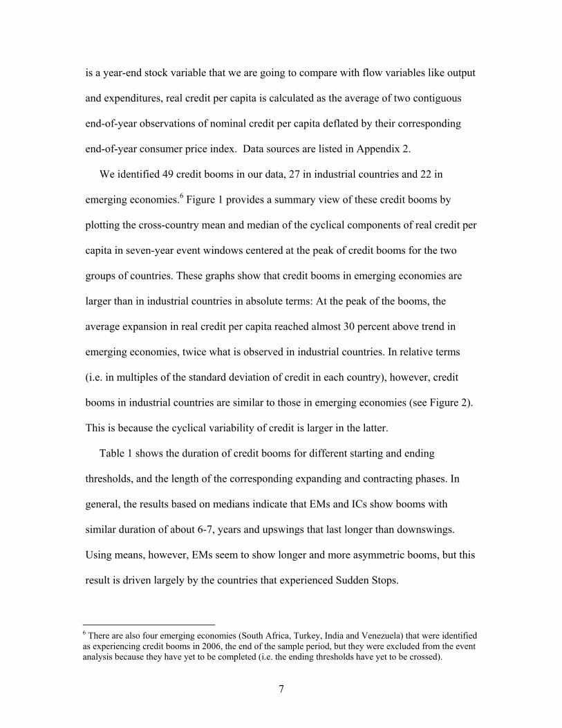
We identified 49 credit booms in our data, 27 in industrial countries and 22 in

emerging economies.6 Figure 1 provides a summary view of these credit booms by

plotting the cross-country mean and median of the cyclical components of real credit per

capita in seven-year event windows centered at the peak of credit booms for the two

groups of countries. These graphs show that credit booms in emerging economies are

larger than in industrial countries in absolute terms: At the peak of the booms, the

average expansion in real credit per capita reached almost 30 percent above trend in

emerging economies, twice what is observed in industrial countries. In relative terms

(i.e. in multiples of the standard deviation of credit in each country), however, credit

booms in industrial countries are similar to those in emerging economies (see Figure 2).

This is because the cyclical variability of credit is larger in the latter.

Table 1 shows the duration of credit booms for different starting and ending

thresholds, and the length of the corresponding expanding and contracting phases. In

general, the results based on medians indicate that EMs and ICs show booms with

similar duration of about 6-7, years and upswings that last longer than downswings.

Using means, however, EMs seem to show longer and more asymmetric booms, but this

result is driven largely by the countries that experienced Sudden Stops.

6 There are also four emerging economies (South Africa, Turkey, India and Venezuela) that were identified as experiencing credit booms in 2006, the end of the sample period, but they were excluded from the event analysis because they have yet to be completed (i.e. the ending thresholds have yet to be crossed).

8

Credit booms tend to be clustered geographically and not limited to a single region:

40 percent of the booms experienced by emerging economies were observed in East Asia

and 32 percent in Latin America. Likewise, 33 percent of the credit booms in industrial

countries were observed in the G7 and 18 percent in the Nordic countries (Denmark,

Finland, Norway, and Sweden). In addition, Figure 3 shows that credit booms tend to be

synchronized internationally and centered around big events—e.g. the Bretton Woods

collapse of the early 1970s, the petro dollars boom in the prelude of the 1980s debt

crisis, the ERM and Nordic country crises of the early 1990s, and the recent sudden

stops. The Figure also suggests that the frequency of credit booms in industrial countries

seems to have declined over time, but this may in fact reflect the pattern of financial

deepening away from banks and into non-bank financial intermediaries, rather than an

actual reduction in the occurrence of credit booms.7 A credit boom driven by non-bank

financial intermediaries would not be captured in the IFS data that we used. 8

2.3 Differences with the method of Gourinchas, Valdes and Landerretche

As noted in the Introduction, several recent studies of credit booms use the thresholds

method proposed by GVL, but their method yields results that differ markedly from ours.

Hence, it is important to explain why the two methodologies produce different results.

Both methods are threshold methods: They define credit booms by identifying periods in

which credit is deemed to have expanded “too much” relative to a long-run trend.

However, the two methods differ in three key respects:

7 For example, Rajan (2005) argues that technical change, deregulation, and institutional change have resulted in an increasing number of arm’s length transactions away from banks in the financial system. 8 Indeed, the growing securitization of subprime mortgages in the United States in recent years was accompanied by an increase in the off-balance sheet operations of bank entities.

9

(1) Measure of credit: We use real credit per capita, while GVL use the ratio of

nominal credit to nominal GDP. The latter has three limitations. One is that it

does not allow for the possibility that credit and output could have different

trends, which is important if countries are undergoing a process of financial

deepening, or if for other reasons the trend of GDP and that of credit are

progressing at different rates. Second, there can be situations when both nominal

credit and GDP are falling and yet the ratio increases because GDP falls more

rapidly. Lastly, when inflation is high, the fluctuations of the credit to GDP ratio

could be misleading because of improper price adjustments.

(2) Detrending procedure: We detrend the credit data using a standard application of

the HP filter to our full sample period 1960-2006 with the value of the HP

smoothing parameter commonly used in annual data (100). In contrast, GVL used

an expanding HP trend with a smoothing parameter of 1000. This expanding trend

extends the sample over which the trend is computed by one year as each

successive year in the sample is added (see Appendix 3 for details).

(3) Definition of thresholds: Our thresholds are defined as multiples of the country-

specific standard deviation of credit over the business cycle, which makes the

threshold level of credit needed to define a boom (i.e. the product ( )ilφσ ) vary

with each country’s cyclical variability of credit. This ensures that a credit boom

is a situation in which the deviation from trend in credit is “unusually large”

relative to a country’s typical credit cycle. In contrast, GVL use a boom threshold

that is invariant across countries, regardless of whether it represents a small or

large change relative to a country’s historical cyclical variability of credit.

10

These differences have significant quantitative implications. To illustrate these

differences, we apply the two methods to the case of Chile, which is also the case that

GVL used to illustrate their method. Figure 4 shows the results of applying our method to

Chilean data. Panel 1 shows results using our method exactly as described in 2.1. It

shows the actual data for the log of real credit per capita, the HP trend, and the boom and

start/end thresholds.9 Panel 2 changes the smoothing parameter from 100 to the value

used by GVL (1000). Panel 3 changes the measure of credit from real credit per capita to

GVL’s ratio of credit to GDP. Panel 4 changes both the smoothing parameter and the

definition of credit for the ones used in GVL, but retains our country-specific thresholds.

Our baseline results in Panel 1 indicate that Chile experienced a credit boom that

peaked in 1981 and lasted five years (from 1979 to 1983). Panel 3 shows that if we use

the credit-GDP ratio as the measure of credit, the boom peaks in 1984 and also lasts five

years (from 1981 to 1985). Thus, under our method the choice of credit variable affects

the timing of the boom but not its duration. In contrast, Panels 2 and 4 show that

increasing the smoothing parameter from 100 to 1000 affects the timing of the boom, and

increases both the size of its peak and its duration. This occurs because a larger

smoothing parameter produces a smoother trend with larger and more persistent

deviations from trend.

Figure 5 conducts a similar experiment as Figure 4 but now starting in Panel 1 with

the results produced by applying the GVL method as proposed in their paper. Panel 2

lowers the smoothing parameter to 100. Panel 3 changes the measure of credit from the

credit-GDP ratio to real credit per capita. Panel 4 changes both the measure of credit and

9 We set the start and end thresholds equal to 1.

11

the smoothing parameter to the ones we used, but retains the country-invariant threshold

proposed by GVL.

The results in Panel 1 of Figure 5 are nearly identical to those obtained by GVL (see

Figure 2b in their paper), confirming that our implementation of their methodology is

accurate. The GVL method indicates that Chile experienced a credit boom that peaked in

1982 and lasted fourteen years (from 1971 to 1984).10 Panels 3 and 4 show that if we

change the credit measure to real credit per capita, the GVL method cannot identify a

credit boom in Chile in the sample period, regardless of the value of the smoothing

parameter. This is because deviations from trend in real credit per capita at least as large

as 19.5 percent were not observed in Chile, and indeed are extremely large relative to the

Chilean history of deviations from trend in real credit per capita. In contrast, our method

adjusts the boom threshold to the observed country cyclical variability of credit. As a

result, our methodology is robust to the choice of measuring credit in real per capita

terms v. as a share of GDP, but the GVL method is not.

Panel 2 of Figure 5 shows that when the expanding HP trend is calculated using a

smoothing parameter equal to 100, the GVL method does identify a credit boom in the

early 1980s, but one that lasted only three years instead of fourteen—again because a

larger smoothing parameter produces a smoother trend with larger and more persistent

deviations from trend. Thus, the higher smoothing parameter used in GVL’s calculations

is the key factor behind the long duration of the credit boom they identified (compare

Panels 1 and 2).

10 GVL dated the peaked on the same year and about the same magnitude, but estimated the duration at 10 years. This difference is due to the longer sample period in our data (which ends in 2006 instead of 1996), and because of data revisions in the credit-to-GDP data relative to our sample.

12

One key additional feature that affects the quantitative implications of the two

methods is that the expanding trend with high smoothing parameter of the GVL method

results in a trend that approximates a smoothed version of the actual time series of credit

with some lag. This point is illustrated in Figure 6, which compares the actual time series

of the credit measures with the standard HP trend (as used in our method) and with the

expanding HP trend (as used in the GVL method). At the beginning and at the end of the

sample the two trends are very similar, but in most of the “internal” periods (and

particularly during the period of fast credit growth) the expanding trend resembles a

smoothed lagged transformation of the original data. Hence, in these periods the

expanding trend treats actual observations of high credit-GDP ratios as being largely part

of the long-run trend of credit, when in reality they are not.

3. Credit Booms and Macroeconomic Dynamics

This Section examines the business cycle behavior of the economy during credit

boom events, and conducts a frequency analysis of the association between credit booms

and financial crises, and between credit booms and three of their potential driving forces

(foreign capital inflows, TFP gains and financial reforms).

3.1 Event analysis

We construct seven-year event windows of the cyclical components of macro

aggregates centered on the peak of credit booms (i.e. t̂ is normalized to date t=0). The

windows show the cross-country means and medians of output (Y), private consumption

(C), public consumption (G), investment (I), the output of nontradables (YN), the real

exchange rate (RER), the current account-output ratio (CAY) and total capital inflows as

share of output (KI). All these variables are at constant prices, expressed in per-capita

13

terms and detrended with the HP filter setting the smoothing parameter at 100, except for

RER (which is not in per-capita terms) and the current account-output and capital

inflows-output ratios (which are at current prices and not expressed in per capita terms).

Data sources are listed in Appendix 2.11

Figures 7-10 illustrate business cycle dynamics around credit boom episodes in

emerging and industrial economies. Except for RER and KI, there is little difference in

the dynamics produced by country means and medians, indicating that the results are not

driven by outliers. Consider first the plots for emerging economies in the right-side of the

Figures. Y, C and G rise 2 to 4 percentage points above trend in the build up phase of the

credit boom, and drop to between 3 to 4 percent below trend in the recessive phase. I, YN

and RER follow a similar pattern but display significantly larger expansions and

recessions. Investment rises up to 18 percent above trend at t=-1 and drops below trend

by a similar amount by t=2. YN rises to about 6½ percent above trend by t=0 and then

drops to almost 3 percent below trend by t=3. The median RER appreciates 9 percent

above trend at t=-1, and drops to a low of about 4 percent below trend when the credit

boom unwinds. CAY displays the opposite pattern: it declines to a deficit of about 2½

percentage points of GDP in the expanding phase of the boom and then rises to a surplus

of 1½ percentage points of GDP in the declining phase. In line with these current account

dynamics, KI rises by up to 3½ percentage points of GDP by t=-1 and then drops by 2¼

percentage points of GDP by t=3.

The plots for industrial countries in the left-side panels of Figures 7-10 show several

similarities with those for emerging economies, but also some important differences.

Output, expenditures and the current account in the industrial countries follow a cyclical 11 Due to data limitations we exclude Jordan from the event analysis.

14

pattern similar to that observed in the emerging economies, but the amplitude of these

fluctuations is smaller, and government consumption shows the opposite pattern (slightly

below trend in the expanding phase and slightly above trend in the contraction phase).

Two important caveats apply to the event study graphs. First, they illustrate the

cyclical dynamics of macro variables, but do not show if these variables themselves are

undergoing a boom (i.e. an unusually large expansion as defined by our thresholds

method). Table 2 provides evidence to examine this issue by listing the fraction of credit

booms associated with booms in output and expenditures that occur in any year inside the

seven-year window of the credit boom events. The results show that between 1/3 to 3/5 of

the credit booms are associated with booms in Y, YN, C, I, and G, and this holds for

emerging and industrial countries, as well as for all the countries together.

The second caveat of the event study graphs is that they show point estimates of

measures of central tendency (means and medians), but do not demonstrate if these

moments are statistically significant. To explore this issue, we run cross-section

regressions of each macro variable for each date of the event window on a constant. The

standard error for the median (mean) is obtained using quintile (OLS) regressions. As

Table 3 shows, the majority of the mean and median estimates shown in the event study

plots for Y, YN, C, and I are statistically significant at the 1 percent confidence level for

industrial and emerging economies. For G, RER and CA/Y, however, many of the

coefficients have large standard errors.

We now study the behavior of inflation, equity prices and housing prices during credit

booms (see Figure 11).12 Industrial countries show negligible changes in inflation, and

rising (falling) equity and housing prices in the build up (declining) phase of credit 12 See Appendix 2 for data sources. Equity prices and housing prices were deflated by the CPI.

15

booms. In emerging economies, inflation tends to spike after the credit booms peak, but

this result is driven by outliers because the mean inflation at t=1 exceeds the median

inflation by a large margin. The median inflation rises only 2 percent above trend. Hence,

credit booms are generally not associated with surges in inflation in either industrial or

emerging economies. Stock and housing prices show the same pattern in emerging

economies as in industrial countries, but note that the rise in equity prices in the upswing

and the decline in housing prices in the downswing are larger in the former.

In summary, the macro event study shows that credit booms across emerging and

industrial economies are associated with a well-defined pattern of economic expansion in

the build-up phase of the booms, followed by contraction in the declining phase. Output,

expenditures, stock prices, housing prices, and the real exchange rate move above trend

in the first phase, and drop below trend in the second phase, and the current account falls

first and then rises. All of this happens without major changes in inflation. Beyond these

similarities, credit booms in emerging and industrial economies differ in four key

respects: (1) the amplitude of the macroeconomic fluctuations is smaller in industrial

countries; (2) government consumption in industrial countries fluctuates very little and

shows the opposite pattern of that in emerging economies; (3) the current account-output

ratio and the (median) capital inflows-output ratio also display smaller changes in

industrial countries, and their timing differs sharply (CAY does not hit its trough in the

build up phase of the credit boom); and (4) fluctuations in the nontradables sector of

industrial countries are much smaller, and RER actually depreciates slightly, instead of

appreciating sharply, in the expansionary phase of credit booms.

16

These differences in the macro features of credit booms across industrial and

emerging economies are consistent with three well-known facts in international business

cycle studies: First, the larger amplitude of the fluctuations displayed by emerging

economies is in line with well-established evidence showing that business cycles are

larger in developing countries (see Mendoza (1995), Kose, Prasad and Terrones (2003),

Neumeyer and Perri (2005)). Second, the striking difference in the behavior of

government purchases is consistent with the evidence produced in the literature on the

procyclicality of fiscal policy in developing countries (see Kaminski, Reinhart, and Vegh

(2005)). Third, the widening current account deficits followed by reversals, and the

booms followed by collapses in the price and output of the nontradables sector, are

consistent with observations highlighted in the Sudden Stops literature (e.g. Calvo

(1998), Mendoza (2007), Caballero and Krishnamurty (2001)). However, it is important

to note that generally these facts have been documented by examining macroeconomic

data without conditioning for credit booms. In contrast, our results apply specifically to

fluctuations associated with credit boom episodes. This is particularly relevant for the

Sudden Stop facts (i.e. the reversals in CAY and the boom-bust cycles in RER and YN),

because most of the Sudden Stops literature emphasizes the role of credit transmission

mechanisms in explaining Sudden Stops.

Our finding that credit booms are associated with a well-defined cyclical pattern in

output and expenditures contrasts sharply with the findings of GVL showing only

ambiguous evidence of this association. Figure 6 in their paper shows a small cycle in

GDP, a decline in GDP growth below trend for the entire duration of credit booms, and

no cycle in consumption.

17

3.2 Regional differences

The aggregates for industrial and emerging economies mask important variation

across country regions. In industrial countries, the Nordic countries show larger

fluctuations in credit and in the macro variables than the G7 (Figures 12-13). In addition,

some of the macro variables in the Nordic countries peak earlier than credit. In the case

of the emerging market regions (Figures 14-15), output and investment fluctuations in

Asia and Latin America are similar, despite the fact that the median credit expansion in

the latter is much larger. The fluctuations in consumption, however, are larger and peak

later in Latin America. The rise (fall) in stock prices in the upswing (downswing) of

credit booms is larger in Latin America, but the current account reversals when the boom

reverts are larger in Asia.

3.3 Frequency analysis

We conduct next a frequency analysis to examine the association between credit

booms and financial crises, and between credit booms and three of their key potential

determinants: capital inflows, productivity gains and financial reforms. Credit booms are

often cited as the culprit behind financial crises, particularly in emerging economies (see

Eichengreen and Arteta, 2002). If this is the case, credit booms should be closely

associated with financial crises. Table 4 shows the percent of banking crises, currency

crises and sudden stops that occurred during the seven-year window of the credit boom

events in emerging economies, industrial countries and all countries combined. The

percent of crises that occurred before, after and at the peak of the credit booms are listed

in separate columns. The dates identifying the occurrence of these crises were obtained

from sources in the empirical literature. The dates of banking crises are from Demirguic-

18

Kunt and Detragiache (2006).13 The dates of currency crises are from Eichengreen and

Bordo (2002).14 The sudden stops dates are from Calvo, Izquierdo, and Mejia (2004).15

Table 4 yields an important result: Credit booms in emerging economies are often

associated with currency crises, banking crises, and sudden stops. About 68 percent of the

credit booms in emerging economies are associated with currency crises, 55 percent with

banking crises, and 32 percent with sudden stops. Most of these crises either preceded or

coincided with the peak of the credit booms, suggesting that many of the booms ended

after a country suffered a crisis. These findings are also at odds with the conclusion in

GVL suggesting that there is virtually no association between credit booms and financial

crises in emerging economies.

Table 4 also shows that, contrary to what we found in emerging economies, credit

booms in industrial countries are only occasionally associated with banking and currency

crises, and there is no association with sudden stops. Moreover, industrial countries in a

credit boom are more likely to experience currency crises than banking crises. The

combined frequency of currency crises before, after or at the peak of credit booms is

slightly over 50 percent, while that for banking crises is 15 percent. In contrast with the

emerging economies, currency crises are more frequent after the peak of credit booms.

Figures 16-17 shows event windows that compare the fluctuations in credit and macro

aggregates of countries that experienced a crisis (i.e. banking crisis, currency crisis, or

13 A banking crisis is defined as a situation in which at least one of the following conditions holds: (1) the ratio of nonperforming assets to total assets of the banking system exceeds 10 percent; (2) the cost of banking system bailouts exceeds 2 percent of GDP; (3) there is large scale bank nationalization as result of banking sector problems; or (4) there are bank runs or new important depositor protection measures. 14 A currency crisis is defined as a situation in which a country experiences a forced change in parity, abandons a currency peg or receives a bailout from an international organization, and at the same time an index of exchange rate market pressure (a weighted average of the depreciation rate, change in short-term interest rate, and percentage change in reserves) rises 1.5 standard deviations above its mean. 15 A sudden stop is defined as a year-on-year fall in capital flows that exceeds 2 standard deviations relative to the mean.

19

sudden stop) with those that did not. The fluctuations in the countries that experienced

crisis are larger and display more abrupt declines than those of the non-crisis countries.

Consider now the frequency analysis of the association between credit booms and

large capital inflows, financial reforms, and TFP gains. Capital inflows are measured as

gross liability flows (i.e. foreign direct investment, portfolio flows, and other investments

liabilities) in percent of GDP, using data from IFS (see Appendix 2). We define a state of

large capital inflows as of date t when the preceding three-year average of capital inflows

ranked on the top quartile of its respective country group (i.e. emerging markets,

industrial countries, or both) over the 1975-2006 period.16 Domestic financial reforms are

measured using the index produced by Abiad, Detragiache, and Tressel (2007). This

index takes values between 0 and 21 and includes information on reserve requirements

and credit controls, interest rate controls, barriers to entry, state ownership, policies on

securities markets, banking regulation, and capital account restrictions. We identify a

country undertaking significant financial reforms as of date t if the preceding three-year

change in this index ranks on the top quartile of its respective country group over the

1975-2002 period. Our measure of TFP is based on standard growth accounting methods

(see, for instance, Klenow and Rodriguez (1997) and Kose, Prasad, and Terrones (2008)),

using labor and investment data from PWT 6.2. A country is identified to have

experienced high TFP growth as of date t if the preceding three-year average of TFP

growth ranked on the top quartile of its respective group over the 1975-2006 period.

Table 5 shows the fraction of credit booms preceded by large capital inflows,

domestic financial reforms, and large TFP gains. Because these factors are often

16 We focus on the preceding three-year average because we are interested in the role of capital inflows (as well as TFP and financial reforms) as potential causes of credit booms, so we are interested in studying if credit booms are preceded by these developments as a form of statistical causality.

20

interconnected and may interact with each other, we compute the frequency of credit

booms that coincided with each factor individually as well as jointly with pairs of two

factors or with all three factors together. For industrial countries, the results indicate that

40 percent of the credit booms followed large TFP gains and 33 percent followed

significant financial reforms. In contrast, in emerging economies we find that over 50

percent of credit booms were preceded by large capital inflows, while TFP gains and

financial reforms play a small role. Thus, credit booms in industrial countries are

preceded by TFP gains and/or domestic financial reforms and to a much lesser extent by

surges in capital inflows, while the opposite is observed in emerging economies.

4. Credit Booms and Firm Level Data

The previous Section established that credit booms are accompanied by a pattern of

economic expansion followed by contraction. This finding raises an important question:

Are the credit booms and the business cycles that accompany them at the macro level

reflected in the financial conditions of firms and banks at the microeconomic level? To

answer this question, we examine in this Section the dynamics of financial indicators of

corporations and banks around credit boom episodes.

As in the macro analysis, we use the credit boom events identified in Section 2 to

construct seven-year event windows of the evolution of firm- and bank-level financial

indicators centered on the years in which credit booms peaked. The firm-level data

correspond to nonfinancial, publicly-traded firms as reported in Worldscope and

Datastream. The sample period is 1980 to 2005 for the industrial countries and 1991 to

2005 for the emerging markets. This restricts our analysis to credit booms dated after

1991 in the emerging markets. Moreover these data have the drawbacks that the coverage

21

is limited to corporations listed in stock exchanges, and that they are reported on a fiscal

year basis, rather than calendar year. Note, however, that there is no other firm-level,

cross-country database with wider coverage available.17

The bank-level data was obtained from Bankscope and it covers the 1995-2005

period.18 These data include balance sheet information for commercial banks, saving

banks, cooperative banks, mortgage banks, medium- and long-term credit banks, and

bank holding companies. The coverage varies from country to country, and since the

sample starts in 1995 our analysis of banking behavior around credit booms is limited to

the last decade. In the analysis below, we do not report bank indicators for the industrial

countries because these countries have experienced only three credit booms since 1995.

It is worth noting, however, that the behavior of these indicators is broadly in line with

that observed in the emerging market economies.

We construct financial indicators for each firm and bank in each country, and focus

on the median firm or bank as country aggregate. Aggregates for emerging and industrial

countries are then generated as medians of the country aggregates. For the firm-level

data, we also construct the breakdown across tradables and nontradables sectors, and

measure sectoral aggregates using the median firm of the corresponding sector.19

4.1 Firm-level indicators

17 The data are corrected for the presence of multiple listings (firms with multiple country listings are assigned only to the country of primary listing), dead stocks (companies that go out of business are taken out from the sample), and outliers (which can be due to either inadequate accounting, as in the case of firms listed with negative market capitalizations, or statistical outliers, observations that are in excess of two standard deviations from the mean observation). 18 The data are corrected for the presence of the central bank and government and multilateral institutions as well as for outliers (either because of inadequate accounting or extreme values). 19 The nontradables sector includes the following industries: construction; printing and publishing; recreation; retailers; transportation; utilities; and miscellaneous, and the tradables sector includes aerospace; apparel; automotive; beverages; chemical; electrical; electronics; metals; among others.

22

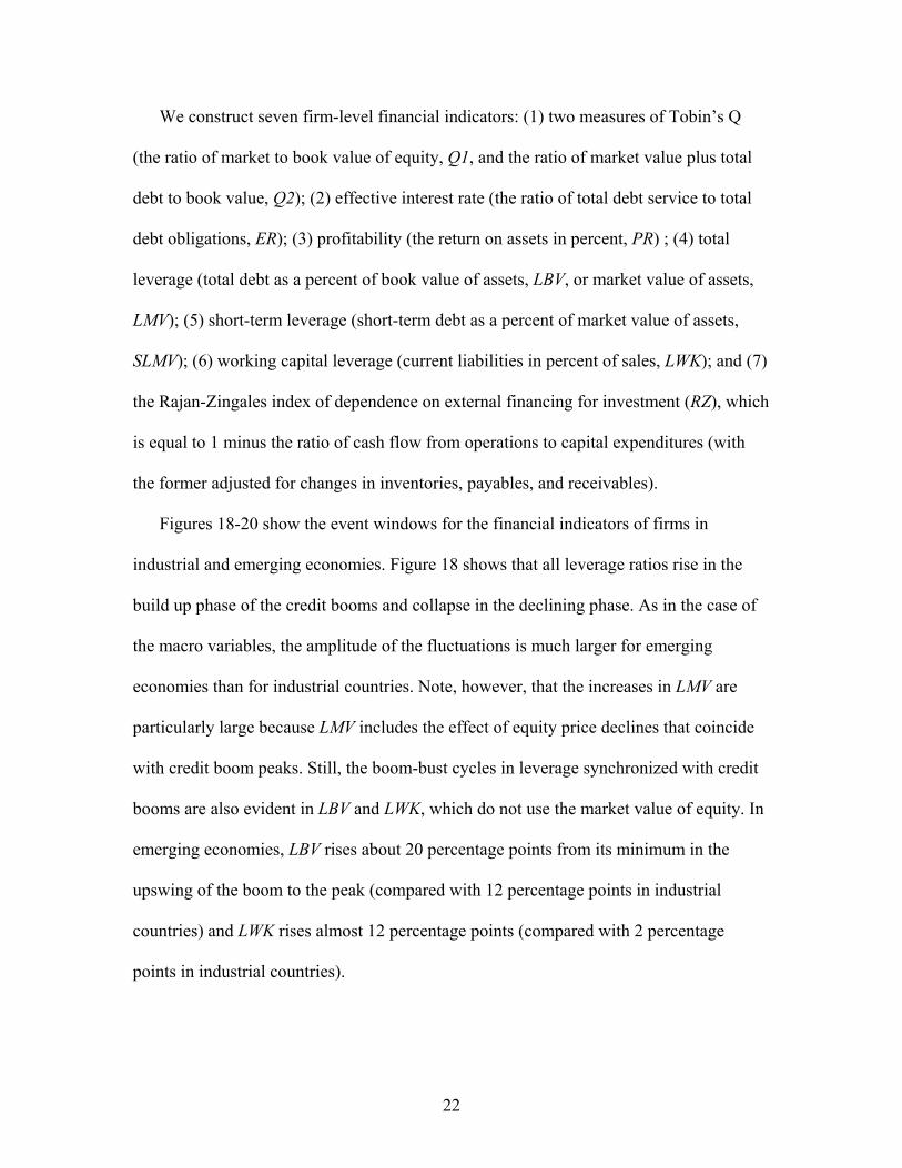
We construct seven firm-level financial indicators: (1) two measures of Tobin’s Q

(the ratio of market to book value of equity, Q1, and the ratio of market value plus total

debt to book value, Q2); (2) effective interest rate (the ratio of total debt service to total

debt obligations, ER); (3) profitability (the return on assets in percent, PR) ; (4) total

leverage (total debt as a percent of book value of assets, LBV, or market value of assets,

LMV); (5) short-term leverage (short-term debt as a percent of market value of assets,

SLMV); (6) working capital leverage (current liabilities in percent of sales, LWK); and (7)

the Rajan-Zingales index of dependence on external financing for investment (RZ), which

is equal to 1 minus the ratio of cash flow from operations to capital expenditures (with

the former adjusted for changes in inventories, payables, and receivables).

Figures 18-20 show the event windows for the financial indicators of firms in

industrial and emerging economies. Figure 18 shows that all leverage ratios rise in the

build up phase of the credit booms and collapse in the declining phase. As in the case of

the macro variables, the amplitude of the fluctuations is much larger for emerging

economies than for industrial countries. Note, however, that the increases in LMV are

particularly large because LMV includes the effect of equity price declines that coincide

with credit boom peaks. Still, the boom-bust cycles in leverage synchronized with credit

booms are also evident in LBV and LWK, which do not use the market value of equity. In

emerging economies, LBV rises about 20 percentage points from its minimum in the

upswing of the boom to the peak (compared with 12 percentage points in industrial

countries) and LWK rises almost 12 percentage points (compared with 2 percentage

points in industrial countries).

23

The Tobin Q and profitability measures shown in Figure 19 indicate that corporations

in both industrial and emerging economies start the expanding phase of credit booms

from high ratios of asset valuation and profitability, which decline as the credit boom

peaks and then remain depressed in the aftermath. Again the magnitude of these

fluctuations is much larger in emerging economies. In contrast, the dynamics of the

effective interest rate are very different in the two groups of countries. In emerging

markets, ER is low in the expansionary phase of the credit booms, and then jumps about

500 basis points one year after the booms peak. In industrial countries, ER is significantly

more stable, and in fact drops slightly after the credit booms peak.

Figure 20 shows the evolution of the RZ index. Corporations are significantly more

dependent on external financing in the build up phase of credit booms than in the

downswing. The size of the correction in the downswing is much larger in emerging

economies than in industrial countries. This evidence is consistent with the argument of

Calvo et al. (2003) suggesting that “creditless recoveries” after Sudden Stops are possible

in emerging economies because firms adjust to the loss of credit so as to provide internal

financing for operational expenses that were previously financed with outside credit.

Figure 21 illustrates important similarities and differences in the evolution of

corporate financial indicators across regions of emerging economies. Firms in Asia are

significantly more leveraged than their Latin American counterparts, and their leverage

ratios fluctuate more sharply during credit booms. Moreover, Tobin’s Q in Asia falls

sharply in a continuous decline during the entire seven-year window, while in Latin

America it shows an ambiguous pattern and a more modest overall decline. Dependence

24

on external financing falls sharply in both regions in the downswing of credit booms, but

the correction is larger in Latin America than in Asia.

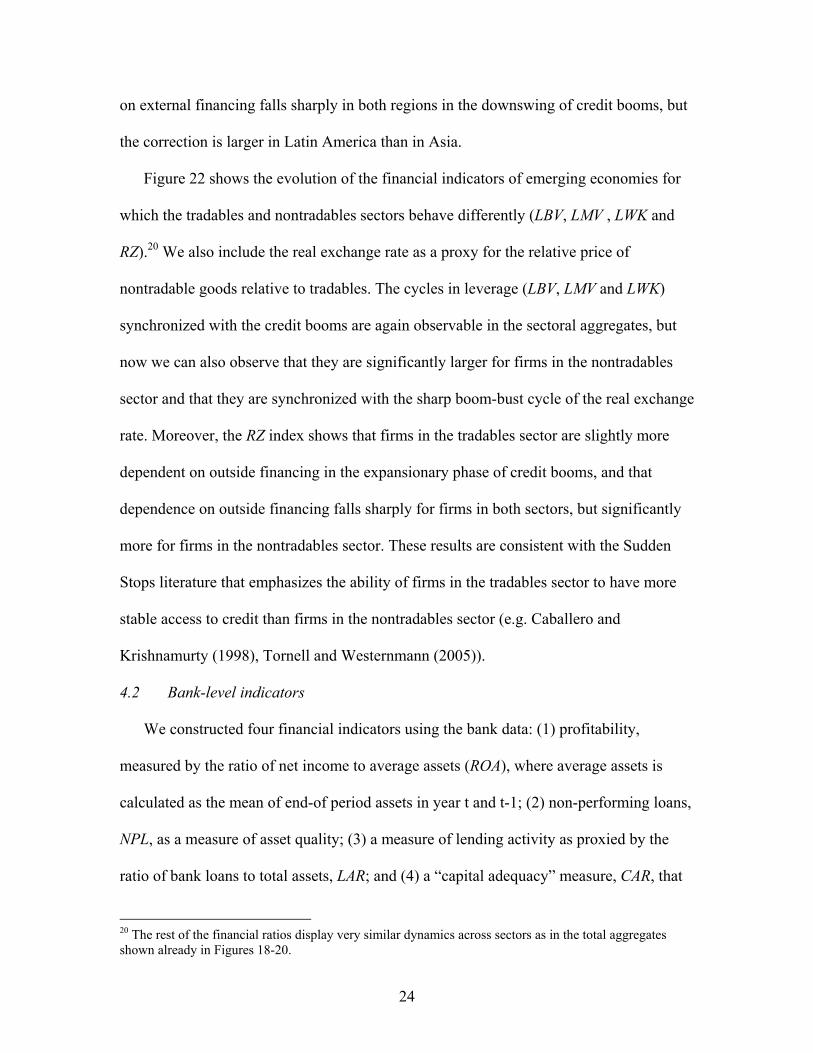
Figure 22 shows the evolution of the financial indicators of emerging economies for

which the tradables and nontradables sectors behave differently (LBV, LMV , LWK and

RZ).20 We also include the real exchange rate as a proxy for the relative price of

nontradable goods relative to tradables. The cycles in leverage (LBV, LMV and LWK)

synchronized with the credit booms are again observable in the sectoral aggregates, but

now we can also observe that they are significantly larger for firms in the nontradables

sector and that they are synchronized with the sharp boom-bust cycle of the real exchange

rate. Moreover, the RZ index shows that firms in the tradables sector are slightly more

dependent on outside financing in the expansionary phase of credit booms, and that

dependence on outside financing falls sharply for firms in both sectors, but significantly

more for firms in the nontradables sector. These results are consistent with the Sudden

Stops literature that emphasizes the ability of firms in the tradables sector to have more

stable access to credit than firms in the nontradables sector (e.g. Caballero and

Krishnamurty (1998), Tornell and Westernmann (2005)).

4.2 Bank-level indicators

We constructed four financial indicators using the bank data: (1) profitability,

measured by the ratio of net income to average assets (ROA), where average assets is

calculated as the mean of end-of period assets in year t and t-1; (2) non-performing loans,

NPL, as a measure of asset quality; (3) a measure of lending activity as proxied by the

ratio of bank loans to total assets, LAR; and (4) a “capital adequacy” measure, CAR, that

20 The rest of the financial ratios display very similar dynamics across sectors as in the total aggregates shown already in Figures 18-20.

25

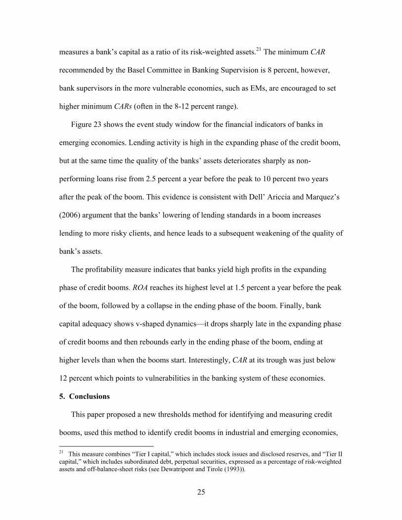
measures a bank’s capital as a ratio of its risk-weighted assets.21 The minimum CAR

recommended by the Basel Committee in Banking Supervision is 8 percent, however,

bank supervisors in the more vulnerable economies, such as EMs, are encouraged to set

higher minimum CARs (often in the 8-12 percent range).

Figure 23 shows the event study window for the financial indicators of banks in

emerging economies. Lending activity is high in the expanding phase of the credit boom,

but at the same time the quality of the banks’ assets deteriorates sharply as non-

performing loans rise from 2.5 percent a year before the peak to 10 percent two years

after the peak of the boom. This evidence is consistent with Dell’ Ariccia and Marquez’s

(2006) argument that the banks’ lowering of lending standards in a boom increases

lending to more risky clients, and hence leads to a subsequent weakening of the quality of

bank’s assets.

The profitability measure indicates that banks yield high profits in the expanding

phase of credit booms. ROA reaches its highest level at 1.5 percent a year before the peak

of the boom, followed by a collapse in the ending phase of the boom. Finally, bank

capital adequacy shows v-shaped dynamics—it drops sharply late in the expanding phase

of credit booms and then rebounds early in the ending phase of the boom, ending at

higher levels than when the booms start. Interestingly, CAR at its trough was just below

12 percent which points to vulnerabilities in the banking system of these economies.

5. Conclusions

This paper proposed a new thresholds method for identifying and measuring credit

booms, used this method to identify credit booms in industrial and emerging economies,

21 This measure combines “Tier I capital,” which includes stock issues and disclosed reserves, and “Tier II capital,” which includes subordinated debt, perpetual securities, expressed as a percentage of risk-weighted assets and off-balance-sheet risks (see Dewatripont and Tirole (1993)).

26

and conducted an event study analysis of the dynamics of macro aggregates and micro-

level financial indicators during credit booms. We identified 27 credit booms in industrial

countries and 22 in emerging economies during the 1960-2006 period. The build up

phase of these booms is associated with economic expansions, rising equity and housing

prices, real currency appreciation, and widening external deficits, followed by the

opposite dynamics in the downswing of the credit booms. Similar dynamics are observed

in firm-level indicators of leverage, firm values, and dependence on external financing,

and in bank-level indicators of asset quality, profitability and lending activity. Moreover,

credit booms tend to be synchronized internationally and centered on “big events” like

the 1980s debt crisis, the 1992 ERM crisis, and sudden stops in emerging economies.

Despite the above similarities in the features of credit booms across industrial and

emerging economies, there are also three major differences: (1) Fluctuations in

macroeconomic aggregates and micro-level indicators during credit booms are larger,

more persistent, and asymmetric in the emerging economies, and this pattern is

particularly strong in the nontradables sector; (2) not all credit booms end in crisis, but

many of the recent emerging markets crises were associated with credit booms; (3) credit

booms in emerging economies tend to be preceded by large capital inflows and not by

domestic financial reforms or TFP gains, while credit booms in industrial countries tend

to be preceded by high TFP or financial reforms. These results differ significantly from

previous findings in the literature on credit booms suggesting an ambiguous relationship

between credit booms and economic expansions, and little or no association between

financial crises and credit booms (see Gourinchas et al. (2001)).

27

The results of our study have important implications for the analysis of macro-finance

linkages, and for surveillance of financial systems and their macroeconomic effects.

From the policy perspective, the thresholds method we proposed provides a tractable

framework for measuring and identifying credit booms that are closely associated with

cyclical fluctuations in macro aggregates and key financial indicators of corporations and

banks. Our results show that credit booms can be identified by the size of a credit

expansion relative to trend, and that this information can be supplemented with other

indicators of excessive credit growth: such as booms in output and expenditures,

excessive real appreciation and/or expansion of the nontradables sector, large inflows of

foreign capital (in EMs) and fast TFP growth or domestic financial reforms (in ICs), as

well as increases in the leverage and profitability ratios of corporations and weakening in

the quality of banks’ assets. Moreover, our results also highlight the importance of using

corrective policy actions to prevent credit booms, because the declining phase of credit

booms is associated with recessions and a higher incidence of financial crises.

From the perspective of research on macro-finance linkages, our results provide a set

of robust empirical regularities that can guide research on models of “credit transmission”

by providing the set of facts that these models should aim to explain. These empirical

regularities can be subsumed into two sets of stylized facts: First, the strong association

of credit booms with booms in output and expenditures, rising asset prices, widening

external deficits and sharp real appreciations. Second, the close relationship between

these macro features of credit booms and a similar cyclical pattern in the financial

indicators of corporations and banks.

28

REFERENCES Abiad, Abdul, Enrica Detragiache, and Thierry Tressel (2007). “A New Database of

Financial Reforms.” Manuscript. Bernanke, Ben and Mark Gertler (1989). “Agency Costs, Net Worth, and Business

Fluctuations,” American Economic Review, Vol. 79, pp. 14-31. Bernanke, Ben, Mark Gertler, and Simon Gilchrist (1999). “The Financial Accelerator in

and Quantitative Business Cycle Framework.” In Handbook of Macroeconomics, Vol. 1C, ed. by John Taylor and Michael Woodford (Amsterdam: North-Holland), pp. 1531-1614.

Borio, Claudio, C. Furfine, and P. Lowe (2001). “Procyclicality of Financial Systems

and Financial Stability.” BIS Papers No.1 (Basle: Bank for International Settlements).

Caballero, Ricardo and Arvind Krshnamurthy (1998). “Emerging Market Crises: An

Asset Markets Perspective.” NBER Working Paper No. 6843. (Cambridge, MA: National Bureau of Economic Research).

Calvo, Guillermo A., Alejandro Izquierdo, and Ernesto Talvi (2003). “Sudden Stops, the

Real Exchange Rate, and Fiscal Sustainability: Argentina’s Lessons.” NBER Working Paper 9828. (Cambridge, MA: National Bureau of Economic Research).

Calvo, Guillermo A., Alejandro Izquierdo, and Luis Mejia (2004). “On the Empirics of

Sudden Stops: The Relevance of Balance-Sheet Effects.” NBER Working Paper 10520. (Cambridge, MA: National Bureau of Economic Research).

Collyns, Charles and Abdelhak Senhadji (2002). “Lending Booms, Real Estate Bubbles,

and the Asian Financial Crisis.” IMF Working Paper 02/20 (Washington: International Monetary Fund).

Corsetti Giancarlo, Paolo Pesenti, and Nouriel Roubini (1999). “What Caused the Asian

Currency and Financial Crisis?” Japan and the World Economy, Vol. 11, pp 305-373,

Cottarelli, Carlo, Giovanni Dell’Ariccia, and I. Vladkova-Hollar (2003). “Early Birds,

Late Risers, and Sleeping Beauties: Bank Credit Growth to the Private Sector in Central and Eastern Europe and the Balkans.” IMF Working Paper 03/213 (Washington: International Monetary Fund).

Dell’Ariccia, Giovanni, and Robert Marquez (2006). “Lending Booms and Lending

Standards.” The Journal of Finance, Vol. 51, No. 5, pp. 2511-2546.

29

Demirguc-Kunt, Asli and Enrica Detragiache (2005). “Cross-Country Empirical Studies of Systemic Bank Distress: A Survey.” IMF Working Paper 05/96. (Washington: International Monetary Fund).

Dewatripont, Mathias and Jean Tirole (1993). The Prudential Regulation of Banks.

(Cambridge, Massachusetts: The MIT Press). Eichengreen, Barry and Michael D. Bordo (2002). “Crises Now and Then: What Lessons

from the Last Era of Financial Globalization?” NBER Working Paper 8716. (Cambridge, MA: National Bureau of Economic Research).

Eichengreen, Barry and Carlos Arteta (2002). “Banking Crises in Emerging Markets:

Presumptions and Evidence,” in Mario Blejer and Marko Skreb (eds.) Financial Policies in Emerging Markets. MIT Press. (Cambridge, Massachusetts).

Fisher, Irving (1933). “The Debt-Deflation Theory of the Great Depressions.”

Econometrica, Vol.1, pp. 337-357. Gorton, Gary and Ping He (2005). “Bank Credit Cycles.” Draft. Gourinchas, Pierre-Olivier, Rodrigo Valdes, and Oscar Landerretche (2001). “Lending

Booms: Latin America and the World.” Economia, Spring, pp. 47-99. Hilbers, Paul, Inci Otker-Robe, Ceyla Pazarbasioglu, and Gudrun Johnsen (2005).

“Assessing and Managing Rapid Credit Growth and the Role of Supervisory and Prudential Policies.” IMF Working Paper 05/151. (Washington: International Monetary Fund).

International Monetary Fund (2004). “Are Credit Booms in Emerging Markets a

Concern?.” World Economic Outlook, pp. 148-166. Kaminsky, Graciela, Carmen Reinhart, and Carlos Vegh (2005). “When it Rains it

Pours: Procyclical Capital Flows and Macroeconomic Policies,” in Mark Gertler and Kenneth Rogoff (eds.) NBER Macroeconomic Annual, pp. 11-53.

Kindleberger, Charles (2000). Manias, Panics, and Crashes: A History of Financial

Crises. (New York: Harcourt, Brace and Company). Kiyotaki, Nobuhiro, and John Moore (1997). “Credit Cycles.” Journal of Political

Economy, Vol. 105, pp. 211-248. Klenow, Peter and Andres Rodriguez-Clare (1997). “The Neoclassical Revival in Growth

Economics: Has It Gone Too Far?” in B. Bernanke and J. Rotemberg (eds.) Macroeconomics Annual 1997, pp. 73-102.

30

Kose, Ayhan, Eswar Prasad, and Marco Terrones (2003). “Financial Integration and Macroeconomic Volatility.” IMF Staff Papers, Vol. 50, pp. 119-143.

Kose, Ayhan, Eswar Prasad, and Marco Terrones (2008). “Does Financial Globalization

Contribute to Productivity Growth?” Mimeo. Kraft, Evan and Ljubinko Jankov (2005). “Does Speed Kill? Lending Booms and their

Consequences in Croatia,” Journal of Banking and Finance, Vol 29, pp. 105-121. Lorenzoni, Guido (2005). “Inefficient Credit Booms.” Manuscript. MIT. Mendoza, Enrique G. (1995). “The Terms of Trade, the Real Exchange Rate, and

Economic Fluctuations.” International Economic Review. Vol. 36, pp. 101-137. ——— (2005). “Real Exchange Volatility and the Price of Nontradables in Sudden-Stop

Prone Economies.” Economia, Fall, pp.103-148. ——— (2006). “Endogenous Sudden Stops in a Business Cycle Model with Collateral

Constraints: A Fisherian Deflation of Tobin’s Q.” NBER Working Paper No. 12564; Cambridge, MA: National Bureau of Economic Research.

Montiel, Peter (2001). “What Drives Consumption Booms?.” The World Bank Review,

Vol. 14, No. 3 , pp. 457-480. Neumeyer, Pablo and Fabrizio Perri (2005). “Business Cycles in Emerging Economies:

The Role of Interest Rate.” Journal of Monetary Economics, Vol. 52, pp. 345-380.

Ottens, Daniel, Edwin Lambregts, and Steven Poelhekke (2005). “Credit Booms in

Emerging Market Economies: A Recipe for Banking Crises?.” Manuscript, De Nederlandsche Bank.

Rajan, Raghuram G. (1994). “Why Bank Credit Policies Fluctuate: A Theory and Some

Evidence,” Quarterly Journal of Economics, Vol. 109, pp. 399-441. Rajan, Raghuram G. (2005). “Has Financial Development Made the World Riskier?” In

The Greenspan Era: Lessons for the Future, pp. 313-369. Federal Reserve Bank of Kansas City

Scheneider, Martin and Aaron Tornell (2004). “Bailout Guarantees, Balance Sheet

Effects and Financial Crises.” Review of Economic Studies. Tornell, Aaron, and Frank Westermann (2005). Boom-Bust Cycles and Financial

Liberalization. Cambridge, MA: The MIT Press.

31

Appendix 1

SAMPLE OF COUNTRIES

The sample comprises 21 industrial countries and 28 emerging markets. The timing of the credit booms are within brackets. Industrial countries Australia (AUS, 1989), Austria (AUT, 1972 and 1980), Belgium (BEL, 1980 and 1990), Canada (CAN, 1967), Denmark (DNK, 1987 and 1991), Finland (FIN, 1991), France (FRA, 1991), Germany (DEU, 1973), Greece (GRC, 1972), Ireland (IRL, 1979 and 2000), Italy (ITA, 1973 and 1992), Japan (JPN, 1973), Netherlands (NLD, 1979), New Zealand (NZL, 1974), Norway (NOR, 1988), Portugal (PRT, 1973 and 2001), Spain (ESP), Sweden (SWE, 1990), Switzerland (CHE, 1990), United Kingdom (GBR, 1974 and 1990), and United States (USA, 1999). Emerging Market Economies Algeria (DZA), Argentina (ARG, 1982), Brazil (BRA), Chile (CHL, 1981), Colombia (COL, 1997), Costa Rica (CRI, 1979), Côte d'Ivoire (CIV, 1978), Ecuador (ECU), Egypt (EGY,1982), Hong Kong (HKG, 1998), India (IND,*), Indonesia (IDN, 1997), Israel (ISR, 1979), Jordan (JOR, 1970), Korea (KOR, 1998), Malaysia (MYS, 1997), Mexico (MEX, 1994), Morocco (MAR, 1977), Nigeria (NGA, 1982), Pakistan (PAK, 1986), Peru (PER), Philippines (PHL, 1983 and 1997), Singapore (SGP, 1984), South Africa (ZAF, *), Thailand (THA, 1997), Turkey (TUR, 1997 and *), Uruguay (URY, 1981), and Venezuela, Rep. Bol. (VEN, *). (*) Ongoing credit booms.

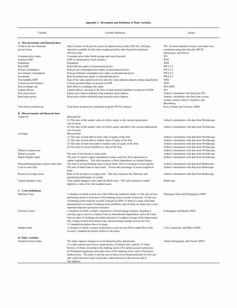
Appendix 2: Description and Definition of Main Variables.

Variable Variable Definition Source

A. Macroeconomic and financial data.Credit to the non-financial Sum of claims on the private sector by deposit money banks (IFS line 22d) plus, IFS. In some industrial country cases data wereprivate sector whenever available for the entire sample period by other financial institutions completed using data from the OECD,

(IFS line 42d). Datastream, and Heaver.Consumer price index Consumer price index (both average and end-of-period). IFSNominal GDP GDP in current prices, local currency. WDIPopulation Population WDIReal GDP Real GDP per-capita, in international prices PWT 6.2Private consumption Real private consumption per-capita, in international prices PWT 6.2Government consumption Real government consumption per-captia, in international prices PWT 6.2Investment Real investment per-capita, in international prices PWT 6.2Non-tradable GDP Sum of the value added in services plus the value added in industry minus manufacture. WDICurrent account balance Current account balance as percent of GDP WDIReal exchange rate Real effective exchange rate, index INS (IMF)Capital inflows Capital inflows (proxied as the flow of total external liabilities) as percent of GDP. IFSReal stock prices Equity price indices deflated using consumer price indeces. Authors' calculation with data from IFS.Real house prices House price indices deflated using consumer price indeces. Authors' calculation with data from several

country sources, Haever Analytics, andBloomberg.

Total factor productivity Total factor productivity calculated using the PWT6.2 dataset Kose, Prasad, and Terrones (2008).

B. Microeconomic and financial data.Tobin's Q Measured by:

(1) The ratio of the market value of a firm's equity to the current replacement Author's calculations with data from Worldscope.cost of assets.(2) The ratio of the market value of a firm's equity and debt to the current replacement Author's calculations with data from Worldscope.cost of assets.

Leverage Measured by:(1) The ratio of total debt to book value of equity of the firm. Author's calculations with data from Worldscope.(2) The ratio of total debt to market value of equity of the firm. Author's calculations with data from Worldscope.(3) The ratio of short term debt to market value of equity of the firm. Author's calculations with data from Worldscope.(4) The ratio of current liabilities to sales of the firm. Author's calculations with data from Worldscope.

Effective interest rate Author's calculations with data from Worldscope.Return on assets The ratio of net income to total assets. Author's calculations with data from Worldscope.Rajan-Zingales index The ratio of a firm's capital expenditures minus cash flow from operations to Author's calculations with data from Worldscope.

capital expenditures. This ratio measures a firm's dependence on extenal finance.Non-performing loans to gross loans ratio The ratio of non-performing loans to gross loans. This is a measure of asset quality. Author's calculations with data from Bankscope.Loan to asset ratio The ratio of bank loans to total assets. Proxies the percentage of assets assigned to Author's calculations with data from Bankscope.

loans.Return on average assets Ratio of net income to average assets. This ratio measures the efficiency and Author's calculations with data from Bankscope.

operational performance of a bank.Capital adequacy ratio Total capital adequacy ratio under the Basle rules. This ratio measures a bank's Bankscope.

capital as a ratio of its risk weighted assets.

C. Crises definitionsBanking Crises A situation in which at least one of the following conditions holds: (1) the ratio of non- Demirguic-Kunt and Detragiache (2006)

performing assets to total asses of the banking sector exceeds 10 percent; (2) the costof banking system bailouts exceeds 2 percent of GDP; (3) there is a large scale banknationalization as result of banking sector problems; and (4) there are bank runs or newimportant depositor protection measures.

Currency Crises A situation in which a country experiences a forced change in parity, abandons a Eichengreen and Bordo (2002)currency peg or receives a bailout from an international organization, and at the sametime an index of exchange rae market pressure (a weighted average of the depreciationrate, change in short-term interest rate, and percentage change in reserves) rises1.5 standard deviations above its mean.

Sudden Stops A situation in which a country experiences a year-on-year fall in capital flows that Calvo, Izquierdo, and Mejia (2004)exceeds 2 standard deviations relative to the mean.

D. Other variablesFinancial reform index The index captures changes in seven financial policy dimensions: Abiad, Detragiache, and Tressel (2007)

(1) credit controls and reserve requirements; (2) Interest rate controls; (3) Entrybarriers; (4) State ownership in the banking sector; (5) Capital account restrictions;(6) Prudential regulations and supervision of the banking sector; and (7) Securitiesmarket policy. The index is just the sum of these seven dimensions(each of wich cantake values between 0 and 3) and takes values between 0 (the lowest) and 21(the highest).

33

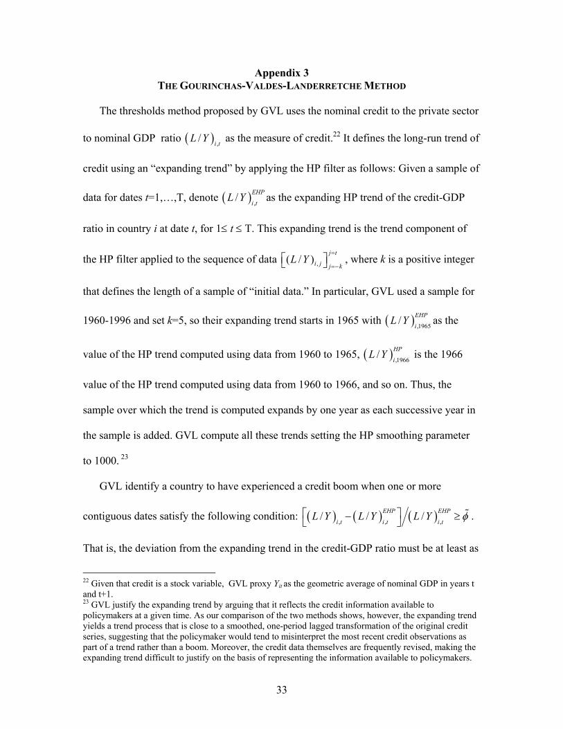
Appendix 3 THE GOURINCHAS-VALDES-LANDERRETCHE METHOD

The thresholds method proposed by GVL uses the nominal credit to the private sector

to nominal GDP ratio ( ) ,/

i tL Y as the measure of credit.22 It defines the long-run trend of

credit using an “expanding trend” by applying the HP filter as follows: Given a sample of

data for dates t=1,…,T, denote ( ) ,/ EHP

i tL Y as the expanding HP trend of the credit-GDP

ratio in country i at date t, for 1≤ t ≤ T. This expanding trend is the trend component of

the HP filter applied to the sequence of data ,( / )j t

i j j kL Y

=

=−⎡ ⎤⎣ ⎦ , where k is a positive integer

that defines the length of a sample of “initial data.” In particular, GVL used a sample for

1960-1996 and set k=5, so their expanding trend starts in 1965 with ( ) ,1965/ EHP

iL Y as the

value of the HP trend computed using data from 1960 to 1965, ( ) ,1966/ HP

iL Y is the 1966

value of the HP trend computed using data from 1960 to 1966, and so on. Thus, the

sample over which the trend is computed expands by one year as each successive year in

the sample is added. GVL compute all these trends setting the HP smoothing parameter

to 1000. 23

GVL identify a country to have experienced a credit boom when one or more

contiguous dates satisfy the following condition: ( ) ( ) ( ), , ,/ / /EHP EHP

i t i t i tL Y L Y L Y φ⎡ ⎤− ≥⎣ ⎦ .

That is, the deviation from the expanding trend in the credit-GDP ratio must be at least as

22 Given that credit is a stock variable, GVL proxy Yit as the geometric average of nominal GDP in years t and t+1. 23 GVL justify the expanding trend by arguing that it reflects the credit information available to policymakers at a given time. As our comparison of the two methods shows, however, the expanding trend yields a trend process that is close to a smoothed, one-period lagged transformation of the original credit series, suggesting that the policymaker would tend to misinterpret the most recent credit observations as part of a trend rather than a boom. Moreover, the credit data themselves are frequently revised, making the expanding trend difficult to justify on the basis of representing the information available to policymakers.

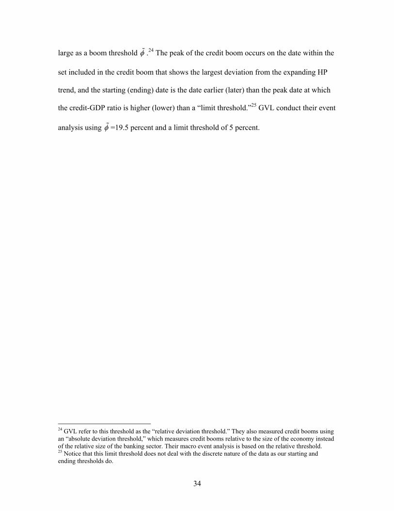
34

large as a boom threshold φ .24 The peak of the credit boom occurs on the date within the

set included in the credit boom that shows the largest deviation from the expanding HP

trend, and the starting (ending) date is the date earlier (later) than the peak date at which

the credit-GDP ratio is higher (lower) than a “limit threshold.”25 GVL conduct their event

analysis using φ =19.5 percent and a limit threshold of 5 percent.

24 GVL refer to this threshold as the “relative deviation threshold.” They also measured credit booms using an “absolute deviation threshold,” which measures credit booms relative to the size of the economy instead of the relative size of the banking sector. Their macro event analysis is based on the relative threshold. 25 Notice that this limit threshold does not deal with the discrete nature of the data as our starting and ending thresholds do.

Figu

re 1

. Cre

dit B

oom

s: S

even

-Yea

r E

vent

Win

dow

s(D

evia

tions

from

HP-

tren

d in

Rea

l Cre

dit P

er-C

apita

)

Indu

stria

l Cou

ntrie

s

Med

ian

Mea

n

-15

-10-505101520253035

-3-2

-10

12

3

Emer

ging

Eco

nom

ies

Med

ian

Mea

n

-10-505101520253035

-3-2

-10

12

3

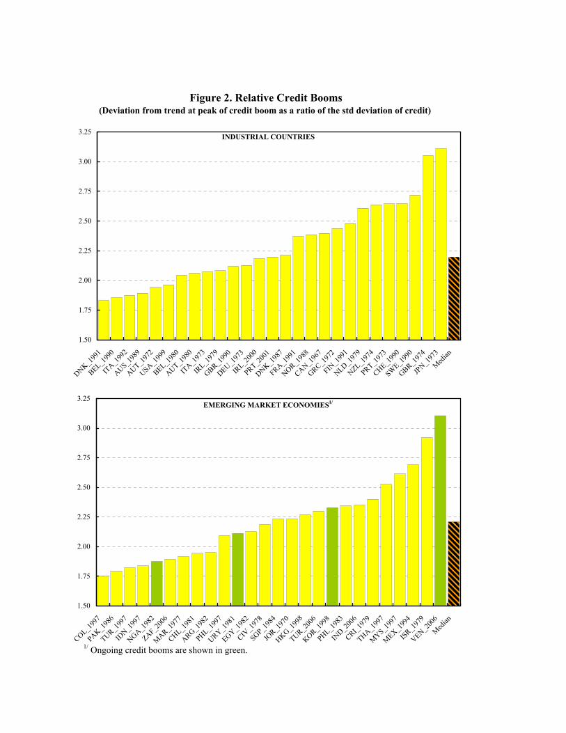
Figure 2. Relative Credit Booms(Deviation from trend at peak of credit boom as a ratio of the std deviation of credit)

1/ Ongoing credit booms are shown in green.

INDUSTRIAL COUNTRIES

1.50

1.75

2.00

2.25

2.50

2.75

3.00

3.25

DNK_199

1

BEL_199

0

ITA_1

992

AUS_198

9

AUT_197

2

USA_199

9

BEL_198

0

AUT_198

0

ITA_1

973

IRL_1

979

GBR_199

0

DEU_197

3

IRL_2

000

PRT_200

1

DNK_198

7

FRA_199

1

NOR_198

8

CAN_196

7

GRC_197

2

FIN_1

991

NLD_197

9

NZL_197

4

PRT_197

3

CHE_199

0

SWE_1

990

GBR_197

4

JPN_1

973

Median

EMERGING MARKET ECONOMIES1/

1.50

1.75

2.00

2.25

2.50

2.75

3.00

3.25

COL_199

7

PAK_198

6

TUR_199

7

IDN_1

997

NGA_198

2

ZAF_200

6

MAR_197

7

CHL_198

1

ARG_198

2

PHL_199

7

URY_198

1

EGY_198

2

CIV_1

978

SGP_198

4

JOR_1

970

HKG_199

8

TUR_200

6

KOR_199

8

PHL_198

3

IND_2

006

CRI_197

9

THA_199

7

MYS_199

7

MEX_199

4

ISR_197

9

VEN_200

6

Median

Figure 3. Frequency of Credit Booms1/

0

1

2

3

4

5

6

7

1967

1969

1971

1973

1975

1977

1979

1981

1983

1985

1987

1989

1991

1993

1995

1997

1999

2001

2003

2005

IND EMEs

?

Bretton WoodsCollapse

Petro-dollar Recycling and Debt Crises

ERM and Nordic Crises

Sudden Stops

1/ Ongoing credit booms are shown in green.

Figure 4. Credit Booms in Chile: the Mendoza-Terrones Method

Real Credit, per capita(Log, Lambda=100)

HP Trend

BoomThreshold

DurationThreshold

8

10

12

14

16

18

1965 1970 1975 1980 1985 1990 1995 2000 2005

Real Credit, per capita(Log, Lambda=1000)

HP Trend

BoomThreshold

Duration Threshold

8

10

12

14

16

18

1965 1970 1975 1980 1985 1990 1995 2000 2005

Credit to GDP ratio(Lambda=100)

HP Trend

BoomThreshold

DurationThreshold

0

10

20

30

40

50

60

70

80

90

1967 1972 1977 1982 1987 1992 1997 2002

Credit to GDP ratio(Lambda=1000)

HP TrendBoomThreshold

DurationThreshold

0

10

20

30

40

50

60

70

80

90

1967 1972 1977 1982 1987 1992 1997 2002

Panel 1 Panel 2

Panel 3 Panel 4

Figure 5. Credit Booms in Chile: the Gourinchas, Valdes, and Landerretche (GVL) Method

Credit to GDP ratio(Lambda=1000)

BoomThreshold

LimitThreshold

0

10

20

30

40

50

60

70

80

90

100

1967 1972 1977 1982 1987 1992 1997 2002

Credit to GDP ratio(Lambda=100)

Boom

Limit

0

10

20

30

40

50

60

70

80

90

100

1967 1972 1977 1982 1987 1992 1997 2002

Real Credit, per capita(Log, Lambda=1000) Boom

Limit

8

9

10

11

12

13

14

15

16

17

18

1967 1972 1977 1982 1987 1992 1997 2002

HP expandingTrend

Real Credit, per capita(Log, Lambda=100)

Boom

Limit

8

9

10

11

12

13

14

15

16

17

18

1967 1972 1977 1982 1987 1992 1997 2002

HPExpandingTrend

HP ExpandingTrend

HP ExpandingTrend

Panel 1 Panel 2

Panel 3 Panel 4

Figure 6. Credit Booms in Chile: Expanding vs. Conventional Trend

Credit to GDP Ratio

0

10

20

30

40

50

60

70

80

90

100

1967 1969 1971 1973 1975 1977 1979 1981 1983 1985 1987 1989 1991 1993 1995 1997 1999 2001 2003 2005

HP ExpandingTrend

HP Trend

Real Credit, per capita(Log)

8

10

12

14

16

1967 1969 1971 1973 1975 1977 1979 1981 1983 1985 1987 1989 1991 1993 1995 1997 1999 2001 2003 2005

HP Expanding

Trend

HP Trend

Figu

re 7

. Cre

dit B

oom

s and

Eco

nom

ic A

ctiv

ity(C

ross

-cou

ntry

mea

ns a

nd m

edia

ns o

f cyc

lical

com

pone

nt o

f rea

l GD

P)

Out

put (

Y)

Med

ian

Mea

n

-5-4-3-2-1012345

-3-2

-10

12

3

Out

put (

Y)

Med

ian

Mea

n

-5-4-3-2-1012345

-3-2

-10

12

3

Indu

stria

l Cou

ntrie

sEm

ergi

ng E

cono

mie

s

Figure 8. Credit Booms and Domestic Demand(Cross-country means and medians of cyclical components)

Consumption (C)

Median

Mean

-5

-4

-3

-2

-1

0

1

2

3

4

5

-3 -2 -1 0 1 2 3

Consumption (C)

Median

Mean

-5

-4

-3

-2

-1

0

1

2

3

4

5

-3 -2 -1 0 1 2 3

Government Consumption (G)

Median

Mean

-5

-4

-3

-2

-1

0

1

2

3

4

5

-3 -2 -1 0 1 2 3

Government Consumption (G)

Median

Mean

-5

-4

-3

-2

-1

0

1

2

3

4

5

-3 -2 -1 0 1 2 3

Investment (I)

Median

Mean

-20

-15

-10

-5

0

5

10

15

20

25

-3 -2 -1 0 1 2 3

Investment (I)

Median

Mean

-20

-15

-10

-5

0

5

10

15

20

25

-3 -2 -1 0 1 2 3

Industrial Countries Emerging Economies

Figure 9. Credit Booms and the Non-tradables Sector(Cross-country means and medians of cyclical components)

Non-tradables Output (YN)

Median

Mean

-6

-4

-2

0

2

4

6

8

-3 -2 -1 0 1 2 3

Non-tradables Output (YN)

Median

Mean

-6

-4

-2

0

2

4

6

8

-3 -2 -1 0 1 2 3

Real Exchange Rate (RER)

Median

Mean

-6

-4

-2

0

2

4

6

8

10

12

-3 -2 -1 0 1 2 3

Median

Mean

-6

-4

-2

0

2

4

6

8

10

12

-3 -2 -1 0 1 2 3

Real Exchange Rate (RER)

Industrial Countries Emerging Economies

Figure 10. Credit Booms, Current Account, and Capital Inflows(Cross-country means and medians of cyclical component)

Current Account-GDP ratio (CAY)

Median

Mean

-3.0

-2.0

-1.0

0.0

1.0

2.0

-3 -2 -1 0 1 2 3

Current Account-GDP ratio (CAY)

Median

Mean

-3.0

-2.0

-1.0

0.0

1.0

2.0

-3 -2 -1 0 1 2 3

Capital Inflows-GDP ratio (KI)

Median

Mean

-3

-2

-1

0

1

2

3

4

5

-3 -2 -1 0 1 2 3

Capital Inflows-GDP ratio (KI)

Median

Mean

-3

-2

-1

0

1

2

3

4

5

-3 -2 -1 0 1 2 3

Emerging EconomiesIndustrial Countries

Figure 11. Credit Booms and Prices(Cross-country means and medians of cyclical components)

Inflation rate

Median

Mean

-6

-4

-2

0

2

4

6

8

-3 -2 -1 0 1 2 3

Inflation rate

Median

Mean

-6

-4

-2

0

2

4

6

8

-3 -2 -1 0 1 2 3

Real stock prices

Median

Mean

-30

-20

-10

0

10

20

30

40

-3 -2 -1 0 1 2 3

Real stock prices

Median

Mean

-30

-20

-10

0

10

20

30

40

-3 -2 -1 0 1 2 3

Real house prices

Median

Mean

-15

-10

-5

0

5

10

15

20

-3 -2 -1 0 1 2 3

Real house prices

Median

Mean

-15

-10

-5

0

5

10

15

20

-3 -2 -1 0 1 2 3

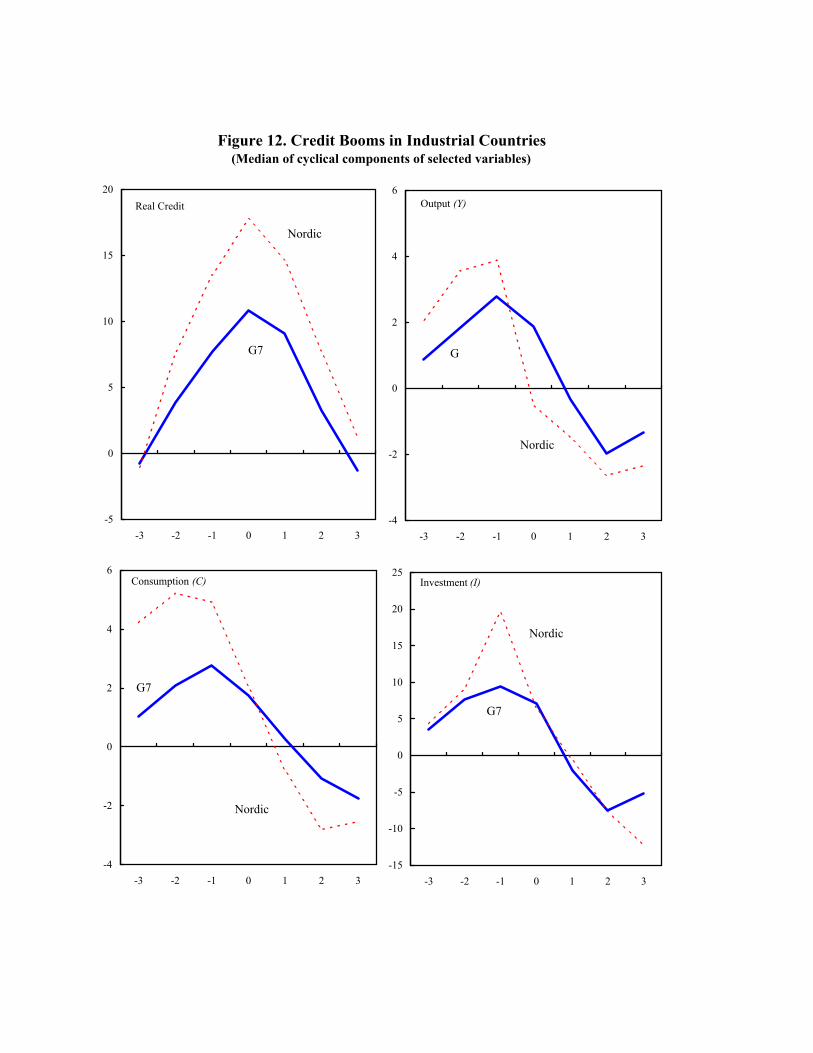
Figure 12. Credit Booms in Industrial Countries(Median of cyclical components of selected variables)

Real Credit

-5

0

5

10

15

20

-3 -2 -1 0 1 2 3

G7

Nordic

Output (Y)

-4

-2

0

2

4

6

-3 -2 -1 0 1 2 3

Nordic

G

Consumption (C)

-4

-2

0

2

4

6

-3 -2 -1 0 1 2 3

Nordic

G7

Investment (I)

-15

-10

-5

0

5

10

15

20

25

-3 -2 -1 0 1 2 3

Nordic

G7

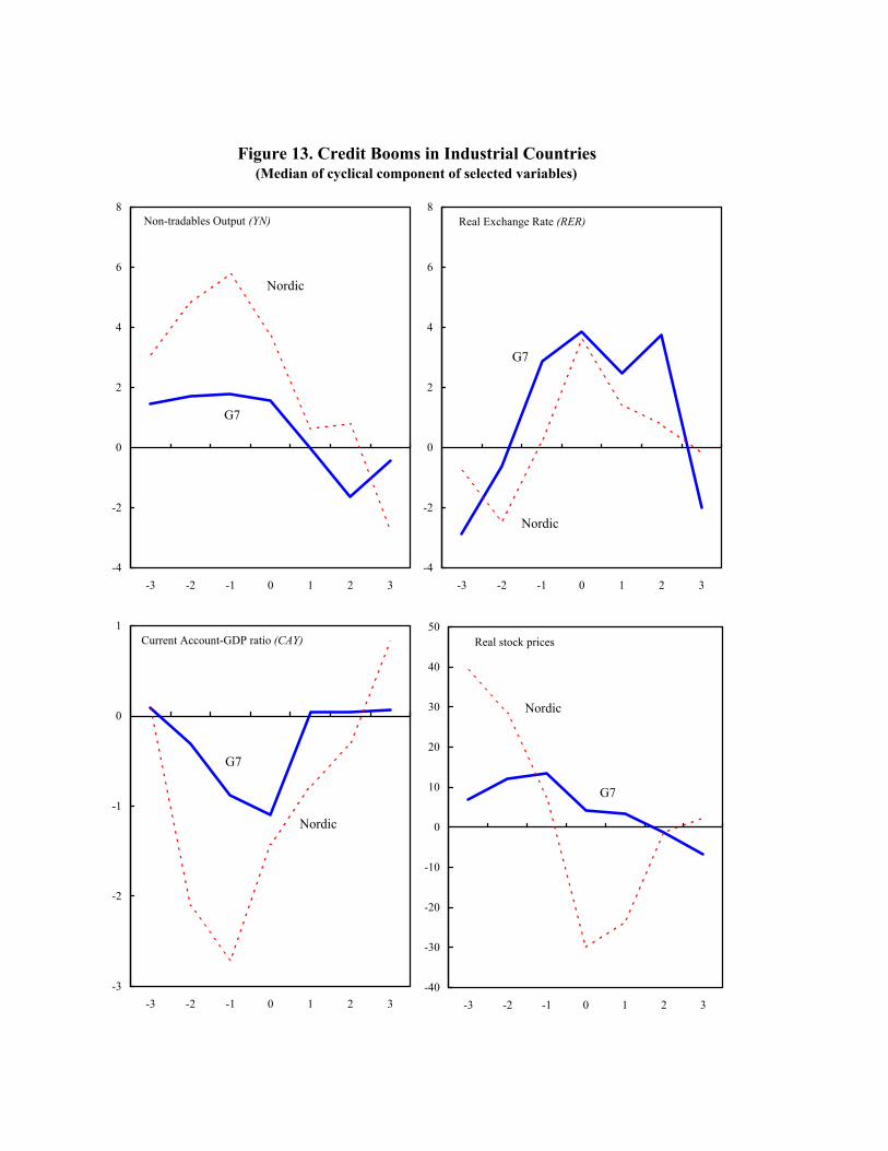
Figure 13. Credit Booms in Industrial Countries(Median of cyclical component of selected variables)

Non-tradables Output (YN)

-4

-2

0

2

4

6

8

-3 -2 -1 0 1 2 3

Nordic

Real Exchange Rate (RER)

-4

-2

0

2

4

6

8

-3 -2 -1 0 1 2 3

G7

Nordic

Current Account-GDP ratio (CAY)

-3

-2

-1

0

1

-3 -2 -1 0 1 2 3

Nordic

G7

Real stock prices

-40

-30

-20

-10

0

10

20

30

40

50

-3 -2 -1 0 1 2 3

G7

Nordic

G7

Figure 14.Credit Booms: Emerging Markets(Median of cyclical component of selected macroeconomic variables)

Real Credit

-10

0

10

20

30

40

50

-3 -2 -1 0 1 2 3

LA

Asia

Output (Y)

-8

-6

-4

-2

0

2

4

6

8

10

-3 -2 -1 0 1 2 3

LA

Asia

Consumption (C)

-8

-6

-4

-2

0

2

4

6

8

10

-3 -2 -1 0 1 2 3

LA

Asia

Investment (I)

-30

-20

-10

0

10

20

30

-3 -2 -1 0 1 2 3

LA

Asia

Figure 15. Credit Booms: Emerging Markets (Median of cyclical component of selected macroeconomic variables)

Non-tradables Output (YN)

-4

-2

0

2

4

6

8

-3 -2 -1 0 1 2 3

LA

Asia

Real Exchange Rate (RER)

-10

-5

0

5

10

15

20

-3 -2 -1 0 1 2 3

LA

Asia

Current Account-GDP ratio (CAY)

-4

-2

0

2

4

-3 -2 -1 0 1 2 3

Asia

LA

Real stock prices

-60

-40

-20

0

20

40

60

80

-3 -2 -1 0 1 2 3

LA

Asia

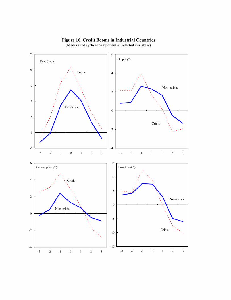
Figure 16. Credit Booms in Industrial Countries(Medians of cyclical component of selected variables)

Real Credit

-5

0

5

10

15

20

25

-3 -2 -1 0 1 2 3

Non-crisis

Crisis

Output (Y)

-4

-2

0

2

4

6

-3 -2 -1 0 1 2 3

Non -crisis

Crisis

Consumption (C)

-4

-2

0

2

4

6

-3 -2 -1 0 1 2 3

Non-crisis

Crisis

Investment (I)

-15

-10

-5

0

5

10

15

-3 -2 -1 0 1 2 3

Crisis

Non-crisis

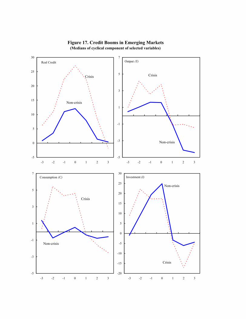
Figure 17. Credit Booms in Emerging Markets(Medians of cyclical component of selected variables)

Real Credit

-5

0

5

10

15

20

25

30

-3 -2 -1 0 1 2 3

Non-crisis

Crisis

Output (Y)

-5

-3

-1

1

3

5

7

-3 -2 -1 0 1 2 3

Crisis

Non-crisis

Consumption (C)

-5

-3

-1

1

3

5

7

-3 -2 -1 0 1 2 3

Crisis

Non-crisis

Investment (I)

-20

-15

-10

-5

0

5

10

15

20

25

30

-3 -2 -1 0 1 2 3

Non-crisis

Crisis

Figure 18. Credit Booms: Corporate Leverage

Total Debt to Book Value of Equity (LBV)

20

30

40

50

60

70

80

90

-3 -2 -1 0 1 2 3

Industrial Countries

Emerging Markets

Total Debt to Market Value of Equity (LMV)

20

30

40

50

60

70

80

90

-3 -2 -1 0 1 2 3

Industrial Countries

Emerging Markets

Short Term Debt to Market Value of Equity (SLMV)

5

10

15

20

25

30

35

40

-3 -2 -1 0 1 2 3

Industrial Countries

Emerging Markets

Current Liabilities to Sales (LWK)

20

30

40

50

60

-3 -2 -1 0 1 2 3

Industrial Countries

Emerging Markets

Figure 19. Credit Booms: Tobin's Q, Interest Rate, and Profitability

Tobin's Q (Q1)

0.40

0.60

0.80

1.00

1.20

1.40

1.60

1.80

2.00

-3 -2 -1 0 1 2 3

Emerging Markets

Tobin's Q (Q2)

0.40

0.60

0.80

1.00

1.20

1.40

1.60

-3 -2 -1 0 1 2 3

Industrial Countries

Emerging Markets

Effective Interest Rate (ER)

6

8

10

12

14

-3 -2 -1 0 1 2 3

Emerging Markets

Industrial Countries

Return on Assets (PR)

3.5

4.5

5.5

6.5

7.5

8.5

-3 -2 -1 0 1 2 3

Industrial Countries

Emerging Markets

Industrial Countries

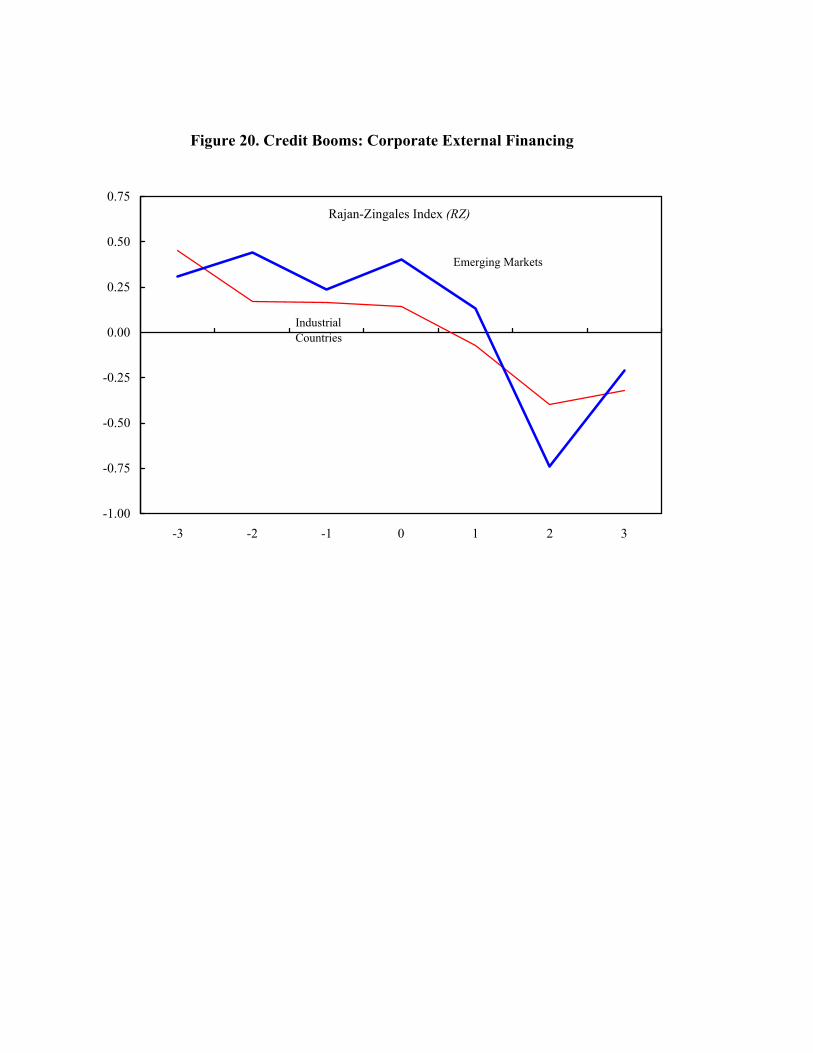
Figure 20. Credit Booms: Corporate External Financing

Rajan-Zingales Index (RZ)

-1.00

-0.75

-0.50

-0.25

0.00

0.25

0.50

0.75

-3 -2 -1 0 1 2 3

Industrial Countries

Emerging Markets

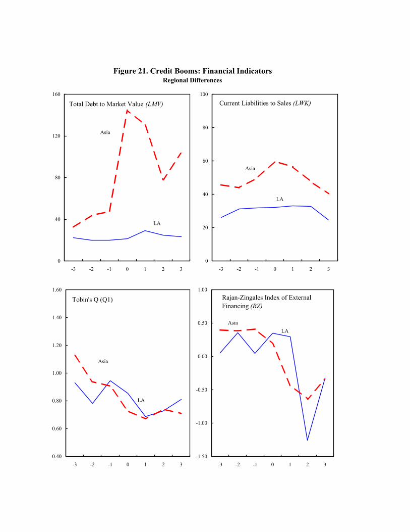
Figure 21. Credit Booms: Financial IndicatorsRegional Differences

Current Liabilities to Sales (LWK)

LA

Asia

0

20

40

60

80

100

-3 -2 -1 0 1 2 3

Tobin's Q (Q1)

LA

Asia

0.40

0.60

0.80

1.00

1.20

1.40

1.60

-3 -2 -1 0 1 2 3

Total Debt to Market Value (LMV)

LA

Asia

0

40

80

120

160

-3 -2 -1 0 1 2 3

Rajan-Zingales Index of External Financing (RZ)

LAAsia

-1.50

-1.00

-0.50

0.00

0.50

1.00

-3 -2 -1 0 1 2 3

Figure 22. Credit Booms: Corporate Leverage and ExternalFinancing in Emerging Market Countries

Total Debt to Book Value ofEquity (LBV)

Non-Tradable

Sector

Tradable Sector

RER (Right Axis)

20

25

30

35

40

45

50

55

60

65

-3 -2 -1 0 1 2 3-10

-5

0

5

10

15

20

Total Debt to Market Value of Equity (LMV)

RER (Right Axis)

10

20

30

40

50

60

70

80

90

100

110

-3 -2 -1 0 1 2 3-10

-5

0

5

10

15

20

Non-Tradable Sector

Current Liabilities to Sales (LWK)

RER (Right Axis)

30

35

40

45

50

55

60

-3 -2 -1 0 1 2 3-10

-5

0

5

10

15

20

TradableSector

Rajan-Zingales Index of External Financing (RZ)

RER (Right Axis)

-2.00

-1.50

-1.00

-0.50

0.00

0.50

1.00

1.50

-3 -2 -1 0 1 2 3-10

-5

0

5

10

15

20

Non-Tradable Sector

Non-Tradable Sector

TradableSector

TradableSector

Figure 23. Credit Booms: Bank Level DataEmerging Market Economies

Asset Quality

NPL

0

2

4

6

8

10

12

-2 -1 0 1 2 3

Credit Operations

50

55

60

65

-2 -1 0 1 2 3

Profiability

ROA

0.6

0.8

1

1.2

1.4

1.6

-2 -1 0 1 2 3

Capital Adequacy

CAR

11

12

13

14

15

-2 -1 0 1 2 3

Tabl

e 1.

Cre

dit B

oom

s: D

urat

ion

Star

ting

and

Endi

ngTh

resh

olds

Dur

atio

nU

psw

ing

Dow

ntur

nD

urat

ion

Ups

win

gD

ownt

urn

A. M

ean

0.00

7.76

0.47

0.40

6.93

0.41

0.45

0.25

7.00

0.47

0.39

6.30

0.41

0.44

0.50

6.05

0.46

0.38

5.63

0.39

0.43

0.75

5.24

0.43

0.38

5.00

0.40

0.40

1.00

4.62

0.41

0.37

4.67

0.39

0.40

B. M

edia

n0.

007.

000.

570.

437.

000.

430.

430.

257.

000.

430.

296.

000.

500.

330.

506.

000.

500.

336.

000.

330.

330.

755.

000.

400.

405.

000.

400.

401.

005.

000.

400.

404.

000.

500.

50

Emer

ging

Mar

ket E

cono

mie

sIn

dust

rial C

ount

ries

Frac

tion

spen

t in

Frac

tion

spen

t in

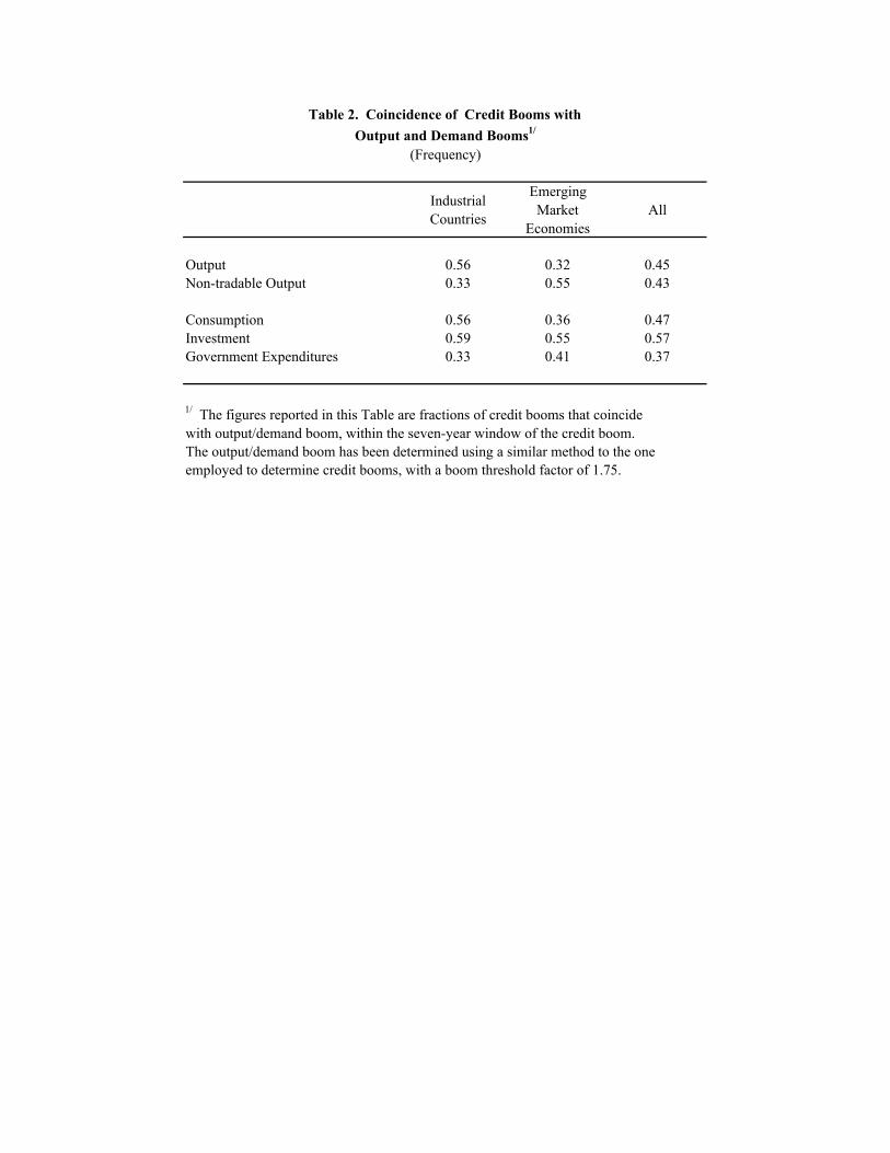
Table 2. Coincidence of Credit Booms withOutput and Demand Booms1/

(Frequency)

Industrial Countries

Emerging Market

EconomiesAll

Output 0.56 0.32 0.45Non-tradable Output 0.33 0.55 0.43

Consumption 0.56 0.36 0.47Investment 0.59 0.55 0.57Government Expenditures 0.33 0.41 0.37

1/ The figures reported in this Table are fractions of credit booms that coincide with output/demand boom, within the seven-year window of the credit boom. The output/demand boom has been determined using a similar method to the oneemployed to determine credit booms, with a boom threshold factor of 1.75.

Tab

le 3

. C

redi

t Boo

ms:

Sta

tistic

al S

igni

fican

ce o

f Eve

nt-W

indo

w C

oeff

icie

nts.

Indu

stri

al C

ount

ries

Em

ergi

ng M

arke

t Eco

nom

ies

t-3t-2

t-1t-0

t+1

t+2

t+3

t-3t-2

t-1t-0

t+1

t+2

t+3

1. M

ean

Val

ues

Rea

l cre

dit

-0.0

27**

0.02

6**

0.10

3***

0.14

1***

0.09

8***

0.03

2**

-0.0

120.

004

0.08

1**

0.20

2***

0.28

3***

0.22

4***

0.05

8-0

.064

*(0

.013

)(0

.013

)(0

.012

)(0

.012

)(0

.012

)(0

.013

)(0

.013

)(0

.034

)(0

.034

)(0

.033

)(0

.032

)(0

.035

)(0

.036

)(0

.036

)O

utpu

t0.

007

0.01

6***

0.03

0***

0.03

1***

0.01

2***

-0.0

12**

-0.0

19**

*0.

007

0.02

2**

0.03

7***

0.03

2***

-0.0

11-0

.026

***

-0.0

25**

*(0

.005

)(0

.005

)(0

.005

)(0

.005

)(0

.005

)(0

.005

)(0

.005

)(0

.009

)(0

.009

)(0

.009

)(0

.009

)(0

.01)

(0.0

1)(0

.01)

Non

-trad

able

Out

put

0.00

80.

012

0.01

8**

0.02

9***

0.02

2***

0.00

3-0

.011

0.01

10.

044*

**0.

057*

**0.

069*

**0.

016

-0.0

28**

-0.0

28**

(0.0

09)

(0.0

08)

(0.0

08)

(0.0

08)

(0.0

08)

(0.0

08)

(0.0

08)

(0.0

11)

(0.0

11)

(0.0

11)

(0.0

11)

(0.0

12)

(0.0

11)

(0.0

11)

Con

sum

ptio

n0.

005

0.01

8***

0.03

0***

0.02

7***

0.01

3***

-0.0

05-0

.018

***

0.00

30.

024*

*0.

046*

**0.

041*

**-0

.011

-0.0

27**

-0.0

32**

*(0

.005

)(0

.005

)(0

.005

)(0

.005

)(0

.005

)(0

.005

)(0

.005

)(0

.011

)(0

.011

)(0

.011

)(0

.011

)(0

.012

)(0

.012

)(0

.012

)G

over

nmen

t Con

sum

ptio

n-0

.007

*-0

.002

0.00

40.

007*

0.00

9**

0.00

9**

0.00

2-0

.001

0.01

20.

036*

**0.

031*

*0.

010

0.00

2-0

.014

(0.0

04)

(0.0

04)

(0.0

04)

(0.0

04)

(0.0

04)

(0.0

04)

(0.0

04)

(0.0

13)

(0.0

13)

(0.0

13)

(0.0

13)

(0.0

14)

(0.0

14)

(0.0

14)

Inve

stm

ent

0.02

60.

063*

**0.

112*

**0.

121*

**0.

024

-0.0

64**

*-0

.075

***

0.01

50.

129*

**0.

191*

**0.

177*

**-0

.039

-0.1

53**

*-0

.095

**(0

.017

)(0

.017

)(0

.017

)(0

.016

)(0

.017

)(0

.017

)(0

.017

)(0

.034

)(0

.034

)(0

.034

)(0

.034

)(0

.037

)(0

.037

)(0

.037

)R

EER

-0.0

24*

-0.0

130.

004

0.03

1**

0.01

50.

002

-0.0

050.

035

0.03

30.

060*

*0.

039

0.00

50.

039

0.01

3(0

.014

)(0

.014

)(0

.014

)(0

.014

)(0

.014

)(0

.013

)(0

.012

)(0

.031

)(0

.029

)(0

.027

)(0

.027

)(0

.03)

(0.0

29)

(0.0

28)

Cur

rent

Acc

ount

Bal

ance

0.00

3-0

.003

-0.0

09**

*-0

.021

***

-0.0

11**

*-0

.001

0.00

5-0

.003

-0.0

03-0

.019

***

-0.0

21**

*0.

012

0.00

70.

003

(0.0

04)

(0.0

04)

(0.0

04)

(0.0

03)

(0.0

03)

(0.0

03)

(0.0

03)

(0.0

07)

(0.0

07)

(0.0

07)

(0.0

07)

(0.0

08)

(0.0

08)

(0.0

08)

2. M

edia

n V

alue

s

Rea

l cre

dit

-0.0

15-0

.015

-0.0

15-0

.015

-0.0

15-0

.015

-0.0

150.

010

0.04

8**

0.15

7***

0.26

0***

0.21

2***

0.05

2**

-0.0

19(0

.015

)(0

.015

)(0

.013

)(0

.013

)(0

.013

)(0

.014

)(0

.015

)(0

.022

)(0

.023

)(0

.023

)(0

.023

)(0

.025

)(0

.024

)(0

.024

)O

utpu

t0.

009

0.01

7***

0.03

1***

0.02

8***

0.01

6***

-0.0

10*

-0.0

15**

*0.

004

0.02

3**

0.02

7***

0.03

6***

-0.0

11-0

.014

*-0

.032

***

(0.0

06)

(0.0

06)

(0.0

06)

(0.0

05)

(0.0

06)

(0.0

06)

(0.0

06)

(0.0

09)

(0.0

09)

(0.0

09)

(0.0

09)

(0.0

1)(0

.008

)(0

.008

)N

on-tr

adab

le O

utpu

t0.

007

0.01

30.

023*

**0.

029*

**0.

011

-0.0

04-0

.009

0.01

00.

054*

**0.

052*

**0.

066*

**0.

013

-0.0

16*

-0.0

25**

*(0

.009

)(0

.008

)(0

.008

)(0

.008

)(0

.008

)(0

.008

)(0

.008

)(0

.009

)(0

.008

)(0

.008

)(0

.008

)(0

.009

)(0

.009

)(0

.01)

Con

sum

ptio

n0.

005

0.01

1**

0.03

1***

0.02

2***

0.00

9*-0

.004

-0.0

17**

*0.

003

0.03

5***

0.04

2***

0.04

1***

-0.0

09-0

.023

**-0

.026

***

(0.0

06)

(0.0

06)

(0.0

06)

(0.0

05)

(0.0

05)

(0.0

06)

(0.0

05)

(0.0

09)

(0.0

09)

(0.0

09)

(0.0

09)

(0.0

1)(0

.01)

(0.0

1)G

over

nmen

t Con

sum

ptio

n-0

.010

**-0

.012

***

0.00

30.

009*

*0.

010*

*0.

005

0.00

60.

015

0.01

50.

029*

*0.

031*

**0.

017

0.00

9-0

.022

*(0

.004

)(0

.004

)(0

.005

)(0

.005

)(0

.005

)(0

.005

)(0

.005

)(0

.012

)(0

.012

)(0

.012

)(0

.012

)(0

.012

)(0

.012

)(0

.012

)In

vest

men

t0.

025*

0.04

5***

0.11

1***

0.10

1***

0.02

7*-0

.067

***

-0.0

76**

*0.

035

0.12

8***

0.17

3***

0.16

9***

-0.0

46*

-0.1

34**

*-0

.051

*(0

.014

)(0

.014

)(0

.016

)(0

.016

)(0

.015

)(0

.013

)(0

.014

)(0

.027

)(0

.025

)(0

.027

)(0

.026

)(0

.028

)(0

.029

)(0

.029

)R

EER

-0.0

06-0

.015

0.00

10.

026*

0.01

4-0

.011

-0.0

060.

028

0.05

6**

0.06

7***

0.02

00.

022

-0.0

08-0

.038

(0.0

12)

(0.0

13)

(0.0

12)

(0.0

14)

(0.0

12)

(0.0

1)(0

.01)

(0.0

28)

(0.0

26)

(0.0

25)

(0.0

25)

(0.0

26)

(0.0

26)

(0.0

25)

Cur

rent

Acc

ount

Bal

ance

0.00

3-0

.001

-0.0

09**

-0.0

18**

*-0

.009

***

-0.0

010.

003

-0.0

07-0

.007

-0.0

24**

*-0

.022

***

0.01

5**

0.00

60.

002

(0.0

03)

(0.0

03)

(0.0

03)

(0.0

03)

(0.0

03)

(0.0

03)

(0.0

03)

(0.0

05)

(0.0

04)

(0.0

05)

(0.0

05)

(0.0

06)

(0.0

05)

(0.0

05)

Not

e: S

tand

ard

erro

rs a

re in

bra

cket

s. T

he c

oeff

icie

nts a

re o

btai

ned

by re

gres

sing

eac

h m

acro

econ

omic

agg

rega

te o

n a

cons

tant

. The

sym

bols

*, *

*, a

nd *

** in

dica

te st

atis

tical

sign

ifica

nce

at th

e 10

%,

5%, a

nd 1

% le

vel,

resp

ectiv

ely.

Bef

ore

Peak

Afte

rTo

tal

Bef

ore

Peak

Afte

rTo

tal

Bef

ore

Peak

Afte

rTo

tal

Boo

mB

oom

Boo

m

All

coun

tries

0.15

0.15

0.04

0.33

0.23

0.15

0.23

0.60

0.06

0.06

0.04

0.17

Indu

stria

l Cou

ntrie

s0.

080.

080.

000.

150.

150.

080.

310.

540.

000.

000.

040.

04

Emer

ging

Mar

ket E

cono

mie

s0.

230.

230.

090.

550.

320.

230.

140.

680.

140.

140.

050.

32

1/ C

oinc

iden

ce o

f cre

dit b

oom

s and

fina

ncia

l cris

es in

the

seve

n-ye

ar w

indo

w a

roun

d th

e bo

om.

2/ A

s def

ined

in D

emirg

uic-

Kun

t and

Det

ragi

ache

(200

6).

3/ A

s def

ined

in E

iche

ngre

en a

nd B

ordo

(200

2).

4/ A

s def

ined

in C

alvo

, Izq

uier

do a

nd M

ejia

(200

4).B

anki

ng c

rises

2/C

urre

ncy

cris

es3/

Sudd

en S

tops

4/

Tab

le 4

. C

redi

t Boo

ms a

nd C

rise

s1/

(Fre

quen

cy)

Table 5. Credit Booms: Potential Triggering Factors1/.(Frequency distribution)

Industrial Countries

Emerging Market

EconomiesAll

Large Capital Inflows (A) 2/ 0.27 0.50 0.52Significant Productivity Gains (B) 3/ 0.40 0.17 0.33Large Financial Sector Changes (C ) 4/ 0.33 0.22 0.27Other 0.27 0.39 0.30

Memo items:(A) & (B) 0.07 0.00 0.09(A) & (C ) 0.00 0.06 0.12(B) & (C ) 0.07 0.11 0.09(A) & (B) & (C ) 0.07 0.06 0.06

1/ Because of data availability we have used the 1975-2005 period only.2/ The three-year average of capital inflow before the peak of the boom ranks in the top quartile oftheir corresponding country group.3/ The three-year average of the annual growth rate of TFP before the peak of the boom ranks in thetop quartile of their corresponding country group.4/ The three-year change before the peak of the boom in the financial reform index ranks in the topquartile of their corresponding country group.