Brigham Young UniversityBYU ScholarsArchive

All Theses and Dissertations

2017-03-01

An Analytical Model to Predict the Length ofOxygen-Assisted, Swirled, Coal and BiomassFlamesDavid Arthur AshworthBrigham Young University

Follow this and additional works at: https://scholarsarchive.byu.edu/etd

Part of the Mechanical Engineering Commons

This Thesis is brought to you for free and open access by BYU ScholarsArchive. It has been accepted for inclusion in All Theses and Dissertations by anauthorized administrator of BYU ScholarsArchive. For more information, please contact scholarsarchive@byu.edu, ellen_amatangelo@byu.edu.

BYU ScholarsArchive CitationAshworth, David Arthur, "An Analytical Model to Predict the Length of Oxygen-Assisted, Swirled, Coal and Biomass Flames" (2017).All Theses and Dissertations. 6286.https://scholarsarchive.byu.edu/etd/6286

An Analytical Model to Predict the Length of Oxygen-

Assisted, Swirled, Coal and Biomass Flames

David Arthur Ashworth

A thesis submitted to the faculty of

Brigham Young University in partial fulfillment of the requirements for the degree of

Master of Science

Dale R. Tree, Chair Julie Crockett

David O. Lignell

Department of Mechanical Engineering

Brigham Young University

Copyright © 2017 David Arthur Ashworth

All Rights Reserved

ABSTRACT

An Analytical Model to Predict the Length of Oxygen-Assisted, Swirled, Coal and Biomass Flames

David Arthur Ashworth

Department of Mechanical Engineering, BYU Master of Science

Government regulations to reduce pollutants and increasing environmental awareness

in the power generation industry have encouraged coal power plants to begin firing biomass in their boilers. Biomass generally consists of larger particles which produce longer flames than coal for a given burner. The length of the flame is important in fixed-volume boilers because of its influence on heat transfer, corrosion, deposition, and pollutant formation.

Many pulverized fuel burners employ a series of co-annular tubes with various flows

of fuel and air to produce a stabilized flame. A variable swirl burner with three co-annular tubes, each of variable diameter, has been used to collect flame length data for nearly 400 different operating conditions of varying swirl, fuel type, air flow rate, enhanced oxygen flow rate and oxygen addition location. A model based on the length required to mix fuel and air to a stoichiometric mixture was developed.

Inputs to the model are the flow rates of fuel, air, and oxygen, swirl vane position and

burner geometries. The model was exercised by changing flow rates and burner tube diameters one at a time while holding all others constant. Physical explanations for trends produced were given.

The model also requires two constants, one of which is solved for given a case without

swirl, and the other is found by fitting experimental data. The constants found in this study appear to be accurate exclusive to the BYU burner. Thus burner designers will need to obtain minimal amounts of data to predict constants for their reactor and then employ the model to predict flame length trends.

The resulting correlation predicts 90% of the flame lengths to be within 20% of the

measured value. The correlation provides insights into the expected impact of burner flow rates and geometry changes on flame length which impacts particle burnout, NOx formation and heat transfer.

Keywords: flame length, coal, biomass, oxygen assisted, pulverized fuel, combustion model

ACKNOWLEDGEMENTS

I am very grateful for the education and experience I have gained as a graduate student at

Brigham Young University. My interactions with fellow students, faculty, and staff have all

contributed to my academic success.

I would like to firstly thank Dr. Tree for constant mentoring and hours spent giving me

careful attention and instruction for my personal development and growth. I would like to thank

my colleagues, John Tobiasson, Nathan Day, Steven Owen, and Daniel Ellis in the combustion

lab for their technical support and good examples. I would like to also thank my family,

especially my wife Sherrie for her support of my educational goals and the care she provided for

our three children at home while I spent countless hours and many late nights on campus.

Finally I would like to thank Air Liquide for the funding that made this work possible,

particularly Bhupesh and his colleagues for their communication and in-person visits.

iv

TABLE OF CONTENTS

List of tables.................................................................................................................................. vi

List of figures ............................................................................................................................... vii

Nomenclature ............................................................................................................................... ix

1 Introduction ........................................................................................................................... 1

1.1 Objectives ......................................................................................................................... 2

1.2 Scope ................................................................................................................................ 3

2 Literature Review .................................................................................................................. 4

2.1 Laminar Diffusion Flames ............................................................................................... 4

2.2 Turbulent Flames .............................................................................................................. 6

2.3 Swirled Turbulent Flames ................................................................................................ 8

2.4 Pulverized Solid Fuel Models ........................................................................................ 11

3 Background .......................................................................................................................... 14

3.1 Flame Length Description .............................................................................................. 14

3.2 Model Derivation ........................................................................................................... 16

3.3 Formation of Nitric Oxides (NOx) ................................................................................. 18

3.4 Loss on Ignition (LOI) ................................................................................................... 19

4 Experimental Setup ............................................................................................................. 22

4.1 Combustion Facility ....................................................................................................... 22

4.2 Fuel Analyses ................................................................................................................. 25

4.3 Operating Conditions ..................................................................................................... 26

5 Results and Discussion ........................................................................................................ 28

5.1 NO vs. LOI ..................................................................................................................... 28

5.2 NO vs CO ....................................................................................................................... 30

5.3 LOI vs Flame Length ..................................................................................................... 31

5.4 NO vs Flame Length ...................................................................................................... 35

5.5 Measurement Comparison .............................................................................................. 36

5.6 Volatiles Flame Length .................................................................................................. 37

5.7 Trends in Flame Length Suggested By Model Results .................................................. 39

5.7.1 Primary Fuel Tube Diameter .................................................................................. 40

5.7.2 Secondary Diameter ................................................................................................ 41

5.7.3 Primary Mass Flow ................................................................................................. 42

5.7.4 Secondary Air Mass Flow ....................................................................................... 44

v

5.7.5 Oxygen Enrichment ................................................................................................ 45

5.8 Predicting Empirical Constants ...................................................................................... 47

5.9 Empirical Constants and the Stokes Number ................................................................. 50

5.10 Discussion ...................................................................................................................... 53

6 Summary and Conclusions ................................................................................................. 55

References .................................................................................................................................... 58

APPENDIX A Loss on Ignition (LOI) Procedure .................................................................... 61

APPENDIX B Oxygen Enrichment Constant (C3) .................................................................. 62

vi

LIST OF TABLES

Table 4.1: Measurements taken at each operating condition and associated methods ..................23

Table 4.2: Diameters (cm) of each of the tubes in the Air Liquide burner ....................................24

Table 4.3: Proximate and ultimate analysis (as received), heating value, and mean particle size of five solid fuels .............................................................................................................25

Table 4.4: Test matrix of operating conditions ..............................................................................26

Table 5.1: Values of empirical constants for each fuel ..................................................................47

Table 5.2: Values of empirical constants using the same c1 for all fuels .......................................48

Table 5.3: Values of c1 and c2 using the curve fit with Stokes number .........................................52

Table B.1: Values of all constants for each fuel ............................................................................62

vii

LIST OF FIGURES

Figure 2.1: Schematic diagram of the fuel and air flow of a simple swirled gas flame ................10

Figure 4.1: Schematic of BYU combustion facility and equipment (not to scale) ........................23

Figure 4.2: Cross section of Air Liquide burner (not to scale) ......................................................24

Figure 5.1: NO vs LOI for two fuels (switchgrass and coal) at various swirl values and oxygen addition levels with burner configuration 1S2L3L ....................................................29

Figure 5.2: NO vs LOI for all fuels at various operating conditions .............................................30

Figure 5.3: NO vs CO for all fuels at various operating conditions ..............................................31

Figure 5.4: LOI vs visual flame length for all fuels at various operating conditions ....................32

Figure 5.5: Burnout vs visual flame length for all fuels at various operating conditions ..............33

Figure 5.6: LOI vs visual flame length for switchgrass and coal at various swirl values and oxygen addition levels with burner configuration 1S2L3L ....................................................34

Figure 5.7: LOI vs visual flame length for switchgrass data .........................................................34

Figure 5.8: NO vs visual flame length for all data at various operating conditions ......................36

Figure 5.9: Calculated flame length vs. visual flame length for all data by fuel ...........................37

Figure 5.10: Calculated volatiles flame length vs. visual volatiles flame length for all data by fuel .....................................................................................................................................39

Figure 5.11: Visual or calculated flame length vs primary diameter for medium wood ...............40

Figure 5.12: Visual or calculated flame length vs secondary diameter for medium wood ...........42

Figure 5.13: Predicted flame length vs primary air mass flow ......................................................43

Figure 5.14: Predicted flame length vs fuel mass flow ..................................................................43

Figure 5.15: Predicted flame length vs total primary mass flow. Fuel-to-air ratio in primary stream is held constant ...........................................................................................................44

Figure 5.16: Measured and predicted flame length vs secondary air mass flow ...........................45

Figure 5.17: Measured and predicted flame length as a function of oxygen added to the secondary air. ..........................................................................................................................46

viii

Figure 5.18: Flame length vs center oxygen mass flow.................................................................46

Figure 5.19: Calculated volatiles flame length vs visual volatiles flame length using a global constant c1 for all fuels with unique c2 for each fuel. ..................................................48

Figure 5.20: c2 values vs average particle size for each fuel .........................................................49

Figure 5.21: Calculated vs visual volatiles flame lengths with set values for both constants .......50

Figure 5.22: c1 vs Stokes number for each fuel .............................................................................51

Figure 5.23: c2 vs Stokes number for each fuel .............................................................................52

Figure 5.24: Calculated vs visual volatiles flame lengths with constants that are correlated with the Stokes number ..........................................................................................................53

Figure B.1: Calculated flame length (m) with a third proportionality constant vs visual volatiles flame length .............................................................................................................63

ix

NOMENCLATURE

Abbreviations ASTM American Society for Testing and Materials BFR Burner Flow Reactor BYU Brigham Young University C Carbon CFD Computational fluid dynamics CO Carbon Monoxide CO2 Carbon Dioxide CPD Coal Percolation and Devolatilization °C Degrees Celsius EPA Environmental Protection Agency HCN Hydrogen Cyanide HHV Higher Heating Value kg/hr Kilograms Per Hour kWth Kilowatts of Thermal Power K Kelvin LOI Loss on Ignition m Meters mm Millimeters N2/N Nitrogen NO Nitric Oxide NO2 Nitrogen Dioxide NOx Nitrogen Oxides O2/O Oxygen ppm Parts Per Million μm Microns or Micrometers wt % Weight Percent Wmfa Weight of Ash with Moisture Removed Wcfa Weight of Carbon Free Ash Yash Mass Fraction of Ash

x

Latin Symbols

b Theoretical diameter of recirculation zone c1 Proportionality constant for shearing termc2 Empirical constant for swirl term cs Stoichiometric mixture of fuel to oxidizer dc Diameter of center tube dp Diameter of primary tube Lf Flame length ṁfuel Total mass flow of solid fuel ṁox Total mass flow of oxidizer ṁO2,p Mass flow of oxygen in primary flow ṁO2,c Mass flow of oxygen in center tube ρmix Density of fuel-air mixture in primary flow ρsec Density of air in secondary flow S Swirl number URZ Tangential velocity of secondary flow induced by swirl Vp Velocity of primary flow Vsec Velocity of secondary flow Yfuel,p Mass fraction of fuel in primary flow YO2,sec Mass fraction of oxygen in secondary flow

1

1 INTRODUCTION Energy efficiency and pollutant emissions will always be a major topic of discussion

among scientists and politicians. Pollutants have negative impacts on the environment, global

climate change, and human health. Among the most hazardous atmospheric pollutants, nitrogen

oxides (NO and NO2, or NOx) are well known for their poisonous and smog-promoting

properties. Power plant boilers produce 40% of the NOx emissions from stationary sources [1].

Recent regulations in the United States, such as the Clean Air Act [2] and its amendments, have

been created to ensure cleaner and more efficient energy production. In order to meet new

regulations much effort has been invested into technologies that may reduce NOx in solid,

pulverized fuel-fired boilers. Burner design alone has been shown to significantly reduce NOx

emissions, as well as improve particle burnout [3]. Low NOx burners are one example of an

emerging burner design of recent decades specifically intended to reduce NOx in boilers [4].

However, optimizing these designs can be quite complex, requiring significant amounts of time

and money invested into modeling the process. Computational fluid dynamics (CFD) is

frequently used but requires massive amounts of data processing which becomes very expensive.

Inexpensive and less time intensive models could be beneficial for preliminary design stages of

new burner configurations and for optimal operation of existing burners.

Cofiring biomass with coal is currently a popular option for CO2 reduction. However,

biomass is not pulverized as easily as coal, and larger biomass particles can create longer volatile

2

flames [5]. Owen et. al. [3] demonstrated that longer biomass flames tend to reduce NOx

formation, but also reduce particle burnout. Flame length also affects the dynamics in boilers

including heat transfer, deposition, and corrosion. Altering the fuel composition will change the

flame length, which is problematic for expensive coal boilers originally designed to burn coal.

Rebuilding entire boilers can be financially impractical, but altering burner operation or

redesigning the burners is much more feasible. One option for improved burner operation is the

selective addition of oxygen at various locations and in various flow streams. Another is the

change of burner dimensions and flow rates. To assist the designing of new burners a large set of

empirical data were collected and evaluated relative to NO, LOI, and flame length. A model

explaining trends in the data and correlating trends in flame length as a function of burner

parameters is sought. This work presents such a correlation and provides explanations of the

trends it produces.

1.1 Objectives

The objective of this work is to collect additional flame length data from a wider range of

fuels including switchgrass and coal and to use these data to evaluate and refine the flame length

model originally proposed by Owen et. al. [3]. Visual flame length data will be collected in

BYU’s burner flow reactor and compared to the model’s predicted values for five solid fuels

including various types of biomass and coal. The model is then exercised to show various trends

produced by changing specific burner and flow parameters. NOx and burnout data will also be

examined to illustrate the importance of predicting flame length.

3

1.2 Scope

This work will demonstrate how certain design parameters affect volatile flame length for

solid pulverized fuel combustion. Flame length is measured visually and predicted analytically.

Empirical constants in the model will be derived by error minimization for each fuel. Two fuels;

coal and switchgrass will be added to the existing data set of straw, medium wood and fine wood

previously collected. Measurements will include visual flame length, exhaust NO, CO, CO2 and

O2 concentration and cyclone collection of ash for LOI analysis. No comprehensive combustion

analysis or CFD is included in this work.

4

2 LITERATURE REVIEW This chapter provides a review of previous methods used to predict flame length

categorized by flame type. In the descriptions which follow below, models have been developed

for various types of flames that determine the location of a stoichiometric mixture. This location

is then compared to some type of flame length measurement.

2.1 Laminar Diffusion Flames

Laminar diffusion flames have been probed and modeled extensively for decades because

of the relative simplicity of their geometry and flow and yet a mathematical description of even

the simplest flame and geometry is challenging because of the necessity to describe mass,

energy, momentum, and chemical reactions simultaneously.

Burke and Schumann [6] provided some of the earliest mathematical descriptions of

cylindrical laminar flames. They presented a method to calculate flame length for a circular port

gas burner with co-flowing air. Their model is used to find the length at which the stoichiometric

ratio of fuel and oxygen occurs along the axis of the flame. In their model they assumed that the

axial gas velocity was constant throughout the fuel and surrounding oxidizer thus producing

mixing only by diffusion. The diffusion coefficient of the gas and air is constant. Their model,

confirmed by experimental data, showed that flame length is related to the burner diameter,

5

diffusion coefficient, viscosity, and stoichiometric fuel air ratio but the relationships between

these variables are not easily determined from their result.

Roper [7] observed that while Burke and Schumann’s model was accurate for circular

port burners, it was not accurate for burners of other geometries. Roper still assumed a constant

velocity profile across the radial axis of the flame but modified the assumption by allowing

velocity to change in the axial direction to include acceleration due to buoyancy. Equations were

then derived for flame height for a circular or square port burner and for slot burners controlled

by momentum or buoyancy, or both by superposition. Roper’s [7] results show that flame length

is proportional to volume flow rate and inversely proportional to the diffusion coefficient and

stoichiometric fuel mass fraction in addition to burner geometry relationships. For a given fuel

and ambient conditions, the common factor affecting flame height for each type of flame/burner

is the volumetric flow rate of fuel.

The work of Burke and Schumann [6] and that of Roper [7, 8] are reviewed by Turns [9]

who utilizes the mixture fraction as a scalar quantity in the mass transport equation and develops

fundamental mass, energy, species, and momentum equations for a reacting circular jet. Solving

these equations for the centerline location ( 0) where the mixture is stoichiometric identifies

the flame length. The result is shown in Equation 2.1 where is the volumetric flow rate of

gaseous fuel, is a diffusion coefficient, and , is the stoichiometric mass fraction of fuel.

This indicates that for a given gaseous fuel, flame length is only a function of the volumetric

flow rate of the fuel.

38

1

, (2.1)

6

This equation indicates that if a laminar burner diameter where doubled, the flame length

would remain unchanged because the increased time required to diffuse oxidizer to the center of

the flame would be offset by the increased time for the flow to reach a particular length from the

burner.

Turns proceeds to reference work done by Fay [10] in which density is no longer

assumed to be constant. In this case, the variable-density solution is given by Equation 2.2

wherein flame length is still a function of the volume flow rate as before but is also a function of

the fuel and ambient densities.

38

1

,

1

⁄ (2.2)

The modeling results of Burke and Schumann [6] and Turns [9] ignore the effects of

buoyancy and yet the results tend to match experimental data fairly well. This is because while

buoyancy tends to accelerate the flow increasing the effective volume flow rate QF which would

tend to increase flame length, it also increases the velocity gradient between the fuel and oxidizer

and therefore increases mixing above the pure diffusion assumed in Equation 2.2 which tends to

decrease flame length. Thus, the two effects tend to offset each other for diffusion flames and the

results of Burke and Schumann [6] and Turns [9] are relatively accurate. Laminar diffusion

flames are therefore readily correlated by volume flow rate, fuel stoichiometric mass fraction,

and the diffusion coefficient.

2.2 Turbulent Flames

Although laminar diffusion flames are relatively simple and more easily modeled,

turbulent flames are used much more frequently in industrial applications. Turbulence has

important flow and mixing effects which add a significant amount of complexity to modeling.

7

Shearing between flows can no longer be neglected, i.e. the assumption of a constant velocity

profile is invalid, and the enhanced mixing of turbulent eddies becomes important.

Due to the extreme complexity and apparent randomness of turbulence, analytical models

are often developed through correlations based on experimental data. Turns [11] reviewed the

work of Wohl et al. [12] in 1949 who found that while laminar flames are a function of

volumetric flow rate and independent of initial jet diameter, this is not the case for turbulent

flames. Beyond the laminar-turbulent transition regime, increasing flowrate does not affect flame

length significantly, and the degree to which it affects flame length appears to be dependent on

burner diameter. In fact, for smaller burner diameters flame length remains nearly constant. This

occurs because as flowrate increases, mixing and air entrainment also increases nearly

proportional to flowrate, which shortens the flame and counteracts the lengthening effect of

higher flowrates.

In 1993, Delichatsios [13] performed a study based on work by Becker and Liang [14]

(1978) on the entire range of turbulent vertical flames, from pool fires (buoyancy-driven or

natural convection) to jet flames (momentum-driven or forced convection). This study correlated

visible flame length data with the Froude number of flow. He then developed a “flame Froude

number” for jet flames which includes effects of combustion stoichiometry. From equations

developed by Delichatsios, Turns [11] outlines a simple approach to analytically solve for the

flame length of a fuel jet issuing from a nozzle of diameter, , into ambient air conditions (∞)

as shown in Equations 2.3 through 2.5 where is the flame Froude number, is the fuel

nozzle exit velocity, is stoichiometric mixture fraction, is the fuel density, ∆ is the

characteristic temperature rise from combustion, and ∗ is a dimensionless flame length.

8

/

/ ∆ / (2.3)

∗13.5 /

1 0.07/ (2.4)

∗ / (2.5)

This model shows us that the four primary factors that affect flame length of turbulent

jets are: 1) the relative influence of momentum and buoyancy ( ), 2) stoichiometric mixture

fraction ( ), 3) fuel to air density ratio ( / ), and 4) jet diameter ( ). At large flame Froude

numbers (Frf >> 1) or flames which have strong initial jet momentum, the flame length is

independent of the Frf, and is only dependent on the burner jet diameter (dj) and fuel

stoichiometric mixture fraction, or for a given fuel the flame length is dependent only on the

burner diameter.

Much of the work on turbulent diffusion flames was comprehensively outlined in a recent

publication on predicting the geometry (length, width, and volume) of laminar, turbulent, and

transition jet diffusion flames by Kang et al. [15]. Like most other combustion models

conservation of mass and momentum equations are employed with various assumptions made for

each type of flame.

2.3 Swirled Turbulent Flames

Turbulent flames are often stabilized by adding swirled air around the fuel. Experiments

have shown that swirl also creates shortened, intense flames [16]. As with laminar and turbulent

9

jet flames, the flame length can be calculated by the distance required to entrain enough oxidizer

to create a stoichiometric mixture.

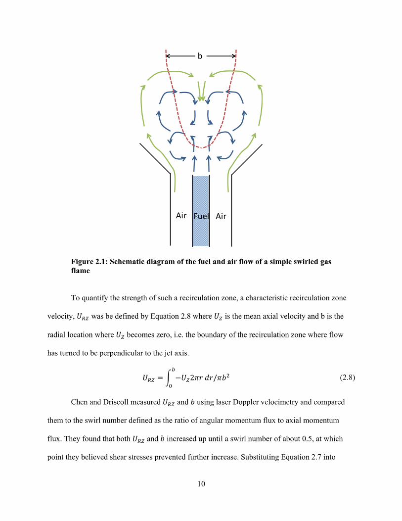
Figure 2.1 shows a schematic diagram of the air and fuel flow velocities of a simple

swirled jet burner. The air is given a tangential velocity which creates a recirculation zone after

exiting the burner. Chen and Driscoll [17] point out that there are two sources of oxidizer

penetration into the fuel rich region. One is by laminar or turbulent diffusion at the boundary of

the fuel and oxidizer jet as is found in laminar and jet diffusion flames. The second is the

entrainment of recirculated oxidizer as shown in Figure 2.1. Recirculating flow at the end of the

recirculation zone travels back toward the burner exit along the axial length of the recirculation

zone. Mixing occurs radially along the axial streams of recirculating oxidizer

The volumetric stoichiometric fuel/air mixture ratio can be created as shown in Equation

2.6 where the numerator is the volumetric flow of fuel exiting the primary fuel tube of diameter

dF at velocity UF, while the numerator is the volume flow rate of the oxidizer mixing into the fuel

stream quantified by a cylindrical volume defined by L and a characteristic mixing velocity

Uc, where L is the flame length, and b is the widest diameter where the average axial velocity is

zero. Thus, the mixing of oxidizer is approximated to occur along a cylindrical boundary of

diameter, b, and length, L.

4

(2.6)

This characteristic mixing velocity is argued to be the sum of two components as shown

in Equation 2.7. The first is due to recirculation while the second is due to shearing between the

fuel and air streams.

| | (2.7)

10

Figure 2.1: Schematic diagram of the fuel and air flow of a simple swirled gas flame

To quantify the strength of such a recirculation zone, a characteristic recirculation zone

velocity, was be defined by Equation 2.8 where is the mean axial velocity and b is the

radial location where becomes zero, i.e. the boundary of the recirculation zone where flow

has turned to be perpendicular to the jet axis.

2 / (2.8)

Chen and Driscoll measured and using laser Doppler velocimetry and compared

them to the swirl number defined as the ratio of angular momentum flux to axial momentum

flux. They found that both and increased up until a swirl number of about 0.5, at which

point they believed shear stresses prevented further increase. Substituting Equation 2.7 into

Air Fuel Air

b

11

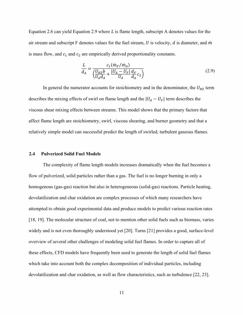
Equation 2.6 can yield Equation 2.9 where is flame length, subscript A denotes values for the

air stream and subscript F denotes values for the fuel stream, is velocity, is diameter, and

is mass flow, and and are empirically derived proportionality constants.

⁄| | (2.9)

In general the numerator accounts for stoichiometry and in the denominator, the term

describes the mixing effects of swirl on flame length and the | | term describes the

viscous shear mixing effects between streams. This model shows that the primary factors that

affect flame length are stoichiometry, swirl, viscous shearing, and burner geometry and that a

relatively simple model can successful predict the length of swirled, turbulent gaseous flames.

2.4 Pulverized Solid Fuel Models

The complexity of flame length models increases dramatically when the fuel becomes a

flow of pulverized, solid particles rather than a gas. The fuel is no longer burning in only a

homogenous (gas-gas) reaction but also in heterogeneous (solid-gas) reactions. Particle heating,

devolatilization and char oxidation are complex processes of which many researchers have

attempted to obtain good experimental data and produce models to predict various reaction rates

[18, 19]. The molecular structure of coal, not to mention other solid fuels such as biomass, varies

widely and is not even thoroughly understood yet [20]. Turns [21] provides a good, surface-level

overview of several other challenges of modeling solid fuel flames. In order to capture all of

these effects, CFD models have frequently been used to generate the length of solid fuel flames

which take into account both the complex decomposition of individual particles, including

devolatilization and char oxidation, as well as flow characteristics, such as turbulence [22, 23].

12

One recent study demonstrated much of the complexity involved in attempting to predict

flame length in solid fuel combustion. Holtmeyer et al. [5] used CFD to model co-fired flames of

pulverized coal and wood waste. Flame length was defined by the point at which CO

concentration was within 15% of its asymptotic value along the axial length of the combustion

chamber. It was discussed that because biomass has a much larger volatile fraction, cofiring with

coal should create longer volatile flames than coal alone. However data showed just the opposite

for biomass cofiring rates below 30%. It was concluded that the most likely cause was larger

biomass particles not releasing volatiles until after passing beyond the coal volatile reaction zone

where the volatiles from coal and smaller wood particles react. This reduces the amount of

gaseous fuel reacting near the burner and thus a shorter volatile flame length. Cofiring rates

beyond 30% appeared to lengthen the flame linearly as larger wood particles began to dominate

combustion behavior, allowing for later volatile release times and less volatile breakthrough.

While CFD models are extremely useful and take into consideration much of the complex

mechanisms of solid particle combustion they are also very computationally intensive and costly.

Simpler models can be useful for predicting trends and understanding fundamental principles

involved in flame length. The purpose of these types of models is not necessarily to accurately

predict the length but to gain insight into how various parameters impact flame length. Kim et al.

[24] created a model that could theoretically predict flame length of single coal particles in a

laminar flow reactor (LFR). Their model is based on balancing mass using a char oxidation rate

equation and numerically solving for a burn-off temperature of a particle. Once the particle

reaches this burn-off temperature it is said to be the tip of the flame for this study. Using a spatial

variation curve for particle temperature fitted to measured data, flame length could be predicted

for a given burn-off temperature. While the model is fairly simple and promising for theoretical

13

prediction of flame length, it requires experimental data of the particle temperature across the

flame and is only applicable to laboratory-scale entrained laminar flow reactor systems. Because

of this and the complexity of the problem analytical models that predict solid fuel flame length

for a wide range of burner sizes and fuels do not currently exist.

14

3 BACKGROUND A flame length model for particle laden flows was initially developed by Owen et. al. [3].

This chapter will review the theory and development of his model as a foundation for

improvements and additional validation to be presented in this work. The chapter begins by

defining a flame and what is typically meant by a flame length. Following this description the

model is then derived. The meaning of each variable and its contribution to the model is

discussed. The processes of NOx formation, carbon burnout will be discussed along with the

impact of swirl on flame shape and length.

3.1 Flame Length Description

A flame is defined as a region over which fuel and oxidizer are converted to products.

Flame thickness, or the physical distance over which a flame reaction occurs is typically on the

order of millimeters. These thin reaction zones form flame sheets, clusters, or wrinkled layers

which surround regions of unburned fuel which are much larger in scale. Thus, a Bunsen burner

flame is a thin annular sheet about 1-2 mm in thickness surrounding a fuel jet several cm in

length. The flame length, unlike the flame thickness is the distance from the burner or fuel exit to

the farthest axial distance where the flame sheet is located. In practice this location is always

somewhat transient, moving closer or further from the burner tip due to perturbations in the flow

and reaction rates.

15

Flame lengths are important for both practical and analytical reasons. In some

applications, a flame is used to transfer heat to a surrounding surface such as the glass making

process. The flame length is therefore an important design parameter and should be made to

match the length of the desired heated surfaces. In other applications the flame may be used to

produce a hot gas such as in a gas turbine engine. Here the flame should be as short as possible

in order to reduce the size and weight of the engine. When a flame impinges on a wall, reactions

can be quenched resulting in undesirable pollutants and perhaps melting or corrosion of the

impacted surface. A knowledge of and the ability to predict flame length can therefore be very

important.

Flame length has been measured by various methods including visual observation,

imaging of visible radiation, temperature measurement, and species measurement. Solid particle

flames provide an additional complication for determining flame length because both the gaseous

volatiles and the solid particles can produce radiation which results in visible emission. In this

work, the flame length was measured by visual observation of the luminous sooting region of

solid particle flames. Soot is produced by the volatile fraction of the fuel and therefore a visible

indication of soot measures only the volatile portion of the flame. Many of the fuel / burner

operating conditions produced particles emission well beyond the volatiles flame length. This

length was not recorded or included in the flame length.

Flame lengths are typically modeled by determining the location where a fuel/oxidizer

mixture is stoichiometric or the mixture fraction of the gases is stoichiometric. The flame length

model developed is therefore an estimate of the length required to mix the volatile fuel with

enough oxidizer to be stoichiometric as has been done for other flames as explained by Turns

16

[25] for laminar and turbulent jet flames and for swirled gaseous flames by Chen and Driscoll

[17].

3.2 Model Derivation

The model as presented here was initially derived by Owen [3] but is repeated here for

clarity and as a starting point for modifications to be added in this work. The model begins with

the stoichiometric ratio of fuel to oxidizer being set equal to a constant cs and shown in

Equation 3.1 where is the total mass flow rate of oxygen in the oxidizer and is the

total mass flow rate of fuel.

(3.1)

The numerator and denominator can be expanded as shown in Equation 3.2. The

numerator represents the fuel flow entering through the primary annulus which for the burner

being used is between the primary tube diameter and the center tube diameter , where ,

is the primary fuel-air mixture density, is the primary mixture velocity, and , is the fuel

mixture fraction of the primary flow. Section 4.1 includes a diagram of the burner being used and

an explanation of where each stream is located.

The denominator consists of four terms each representing a flow of oxygen into the fuel

rich region. The first term follows the nomenclature of Chen and Driscoll [17] and expresses the

radial velocity ( ) along the axial circumference ( ) of the flame. is the flame length,

is the theoretical diameter of the recirculation zone core estimated to be approximately 80% of

the secondary tube diameter, is the density of the secondary air stream and , is the

mass fraction of O2 in the secondary stream. The magnitude of was determined as a function

17

of swirl, , and secondary axial velocity, , based on a correlation of the data from Chen and

Driscoll as shown in Equation 3.3. This correlation was not provided by Chen and Driscoll but

was developed by fitting data from their work relating URZ to swirl. The constant will be

evaluated by experimental results to be shown later.

4 ∗ ,

, , , (3.2)

The second term in the denominator represents oxygen mixing into the fuel jet due to

shearing created by the axial velocity difference between the fuel jet and the secondary flow. The

rate of mixing is assumed to be proportional to the absolute value of the velocity difference of

and , which has been experimentally observed for turbulent flames. The constant must

also be determined by experimental data.

The third term in the denominator , is the flow rate of oxygen in the center tube. The

model assumes that all of the oxygen delivered from this tube is mixed into the fuel stream. In

the experiments used to develop this correlation, the flow exiting this center tube contained pure

oxygen.

The final term in the denominator , is the oxygen contained in the primary stream.

For safety reasons, the oxygen concentration in the primary flow must be maintained near that of

air but in some of the data used to develop the correlation, pure oxygen was premixed into the

primary air-fuel stream within the last 10 cm prior to the burner exit.

Rearranging the terms of Equation 3.2 to solve for the flame length produces

Equation 3.4. The constants and were initially found by minimizing a least squares

0.23 ∗ ∗0.004

(3.3)

18

difference between the measured and predicted flame lengths for each fuel. This provided fuel

specific correlations for flame length.

, ,

,

(3.4)

3.3 Formation of Nitric Oxides (NOx)

NOx is mainly composed of NO which is formed by three chemical mechanisms namely

thermal, prompt, and fuel NOx. Thermal NOx occurs as N2 and O2 dissociate at very high

temperatures (above 1800 K). Atomic N and O then react in what is commonly known as the

extended Zeldovich mechanism [25] shown in Equations 3.5 through 3.7. Previous work at BYU

found that this combustor never exceeds 1800 K outside the flame [26],where the residence time

is long enough to produce the reaction; therefore, this pathway for NO formation is thought to be

negligible.

→ (3.5)

→ (3.6)

→ (3.7)

Prompt NOx occurs very quickly within a flame, and thus its name. CH radicals form

very rapidly during combustion and proceed to react with N2 in the Fenimore mechanism [25]

shown in Equations 3.8 and 3.9. The cyanide compounds formed will proceed to form

intermediate compounds which eventually result in NO. At richer equivalence ratios (> 1.2)

HCN will follow the chain sequence shown in Equations 3.10 through 3.13 to form NO. This

mechanism is thought to contribute to only a small fraction of the NO formed in particle laden

flames because the concentrations of HCN produced are lower than that produced by fuel NOx.

19

→ (3.8)

→ (3.9)

→ (3.10)

→ (3.11)

→ (3.12)

→ (3.13)

Fuel NOx is the dominating mechanism in biomass and coal combustion. Nitrogen is

contained in the fuel’s molecular structure which will quickly convert to HCN or ammonia

(NH3). These products will then follow a path similar to the prompt mechanism outlined above.

It is assumed that this is where the majority of NOx comes from in this work.

3.4 Loss on Ignition (LOI)

Beyond the volatile combustion region, solid fuel particles continue to react in a process

known as char oxidation. To measure the degree of burnout of solid particles after char oxidation

ASTM procedure D3748 was used to determine loss on ignition (LOI), which is an approximate

measure of the amount of carbon left in the ash. The procedure involves heating solids in air at

high temperature. For a detailed step-by-step outline of the ASTM procedure, refer to

APPENDIX A. The majority of the mass released is carbon which oxidizes to produce CO and

CO2. There may however be some mass loss for other elements such as sulfur. LOI is reported as

a fraction of the remaining ash or as a percentage of the mass of the remaining ash. When the ash

fraction of a fuel is very low as is the case for wood, the amount of carbon remaining in the ash

may be a very small fraction of the initial fuel carbon (high burnout) but may still be a large

20

fraction of the remaining ash (high LOI). The smaller the ash fraction, the more difficult it is to

obtain low LOI.

During char oxidation carbon on the surface of the particle reacts with oxygen to form

CO and CO2 via global reactions [25] as shown in Equations 3.14 through 3.17. After immediate

oxidation CO concentration is generally high on the surface of the particles. CO will diffuse

away from the surface and further react with oxygen to form to CO2 as shown in Equation 3.18,

which becomes the final product of carbon in the char.

→ (3.14)

2 → 2 (3.15)

→ 2 (3.16)

→ (3.17)

→ (3.18)

The char oxidation rate is controlled by either temperature (kinetic control) or the

diffusion of oxygen to the surface (diffusion controlled). While both modes can occur in a

particle laden flame, diffusion controlled oxidation tends to dominate until particles become

isolated and cool rapidly in the post flame region. In experiments for this work, once particles

leave the reactor, gas and particle temperature drop rapidly quenching reactions. In fuel rich

regions, char oxidation is reduced as oxygen is consumed by the volatiles more rapidly than by

the char. Thus char oxidation occurs predominantly after the volatile flame and before exiting the

reactor or in the post flame region of the reactor. The final degree to which char oxidation has

progressed by the end of the reactor depends on residence time in this post flame region. Owen

[3] showed that LOI is correlated with flame length. In a fixed volume reactor increasing volatile

21

flame length decreases the length of the burnout zone which reduces the residence time for char

oxidation.

22

4 EXPERIMENTAL SETUP This chapter describes the experimental facilities and equipment used to obtain data for

this work, including NOx, LOI, and flame length measurements. ASTM fuel analyses are also

listed for each solid fuel here.

4.1 Combustion Facility

All experiments were performed in a 150 kWth, cylindrical, down-fired Burner Flow

Reactor (BFR). The full schematic is shown in Figure 4.1. The BFR has an inside diameter of

0.75 m and a height of 2.4 m which consists of six burner sections with heights of 0.4 m. Each

section has four 90 mm x 290 mm access ports 90 degrees apart from one another. Flame length

was observed visually through quartz windows mounted in the access ports on the south side of

the reactor. The windows allowed observation of a large portion of the axial distance of the

flame but the flame was not visible in some locations between windows.

Measurements for this work include exhaust gas concentrations, ash burnout (LOI), and

volatile flame length and are summarized in Table 4.1. Exhaust gas concentrations were

measured using a PG-250 Horiba gas analyzer. This analyzer was capable of measuring NOx,

CO, CO2, and O2. The analyzer was calibrated at the beginning of each day of testing to ensure

accuracy. The exhaust gas line went through an ice bath to condense water before entering the

analyzer. Ash samples were collected on a metal plate at the bottom of a barrel below the

23

cyclone from which LOI measurements were obtained. Volatile flame length was measured by

visual observation via glass windows mounted onto the access ports of the BFR. The windows

were regularly blown off with pressurized air from the inside to improve visibility.

Figure 4.1: Schematic of BYU combustion facility and equipment (not to scale)

Table 4.1: Measurements taken at each operating condition and associated methods

Measurement Units Method

NO ppm

PG-250 Horiba gas analyzer CO ppm

CO2 % vol

O2 % vol

LOI (Loss on Ignition) % mass ASTM Procedure D3748 (See Appendix A) Flame Length meters Visual Confirmation

24

For this work a variable-swirl burner designed by Air Liquide was employed. The burner

consisted of three coaxial tubes allowing for three separate inlet flows, as shown in Figure 4.2.

The diameter of each of the three tubes may be varied by exchanging tubes. Diameters are shown

in Table 4.2 where S, M, and L stand for small, medium, and large respectively. Channel 1

(center) is typically used for the natural gas during preheating. Channel 2 (primary) is typically

used for solid fuel addition conveyed with air from a bulk bag feeder. Channel 3 (secondary) is

used for the secondary air flow that is swirled prior to entering the annulus in a variable swirl

block above the outlet.

Figure 4.2: Cross section of Air Liquide burner (not to scale)

Table 4.2: Diameters (cm) of each of the tubes in the Air Liquide burner

S M L D1 1.905 2.858 3.505 D2 2.667 3.340 4.216 D3 4.272 N/A 5.479 D4 4.826 N/A 6.033 D5 10.795 N/A 13.335

25

4.2 Fuel Analyses

Data for five solid fuels: medium particle size hardwood, fine particle size hardwood,

straw, switchgrass, and sub-bituminous coal, were used in this work. The data for hardwoods and

straw were previously taken by Owen [3]. The ASTM proximate and ultimate analyses of the

five fuels are displayed in Table 4.3.

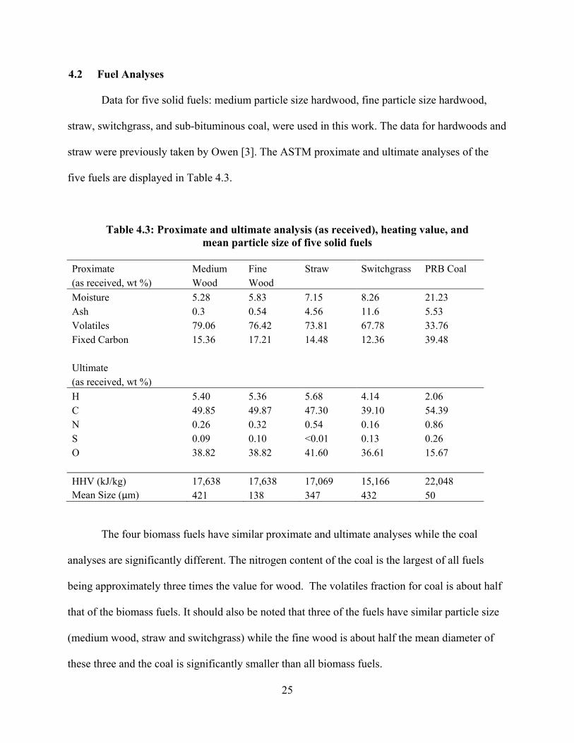
Table 4.3: Proximate and ultimate analysis (as received), heating value, and mean particle size of five solid fuels

Proximate Medium Fine Straw Switchgrass PRB Coal (as received, wt %) Wood Wood

Moisture 5.28 5.83 7.15 8.26 21.23 Ash 0.3 0.54 4.56 11.6 5.53 Volatiles 79.06 76.42 73.81 67.78 33.76 Fixed Carbon 15.36 17.21 14.48 12.36 39.48 Ultimate (as received, wt %)

H 5.40 5.36 5.68 4.14 2.06 C 49.85 49.87 47.30 39.10 54.39 N 0.26 0.32 0.54 0.16 0.86 S 0.09 0.10 <0.01 0.13 0.26 O 38.82 38.82 41.60 36.61 15.67

HHV (kJ/kg) 17,638 17,638 17,069 15,166 22,048 Mean Size (μm) 421 138 347 432 50

The four biomass fuels have similar proximate and ultimate analyses while the coal

analyses are significantly different. The nitrogen content of the coal is the largest of all fuels

being approximately three times the value for wood. The volatiles fraction for coal is about half

that of the biomass fuels. It should also be noted that three of the fuels have similar particle size

(medium wood, straw and switchgrass) while the fine wood is about half the mean diameter of

these three and the coal is significantly smaller than all biomass fuels.

26

4.3 Operating Conditions

Various operating conditions were used for experiments in this work and are summarized

in Table 4.4. The burner configuration 1S2L3L was chosen for these tests because it was the

most frequently used configuration in Owen’s data allowing for a more suitable comparison

between fuels. Oxygen varied from 0 – 16 kg/hr for switchgrass, but only 0 – 8 kg/hr for coal.

This is because at oxygen flow rates above 8 kg/hr in the center tube the high velocity of oxygen

would overtake the coal flame, which is already shorter than any biomass flame, in which the

oxygen flow appeared to destroy the recirculation zone and lead to poor results. Swirl was held

at three different values depending on the number of 360 degree turns of the adjusting screw in

the swirl block. Oxygen addition occurred in both the center tube and secondary flow. In the

secondary flow two cases existed. For the “Constant Air” case oxygen was simply added to the

secondary air flow. For the “Constant O2” case the secondary air was reduced in order to keep

the total mass flow of oxygen into the reactor constant. In other words, since air is made up of

almost 25% oxygen by mass, the secondary air flow would be reduced by about 4 kg/hr for each

kg/hr of additional oxygen flow.

Table 4.4: Test matrix of operating conditions

Fuel Burner

Configuration O2 Flow Rates

(kg/hr) Swirl

(0, 6, 9 Turns) Oxygen Location

Switchgrass 1S2L3L 0, 2, 4, 6, 8, 12, 16 1.44, 1.11, 0.84 Center, Secondary (Constant Air, Constant O2)

Coal 1S2L3L 0, 4, 8 1.44, 1.11, 0.84 Center, Secondary (Constant Air)

In addition to the data taken at BYU, two data points from the University of Utah were

included for comparison. The first data point was taken in their L-1500 furnace. This is a 1.5

MW combustor similar to the BFR which employs a burner with coaxial tubes for firing

27

pulverized coal and/or natural gas. This particular data point was taken with pulverized coal,

similar to that used in BYU tests, fired in air with a swirl number of approximately 1.2. The

second data point was taken in their Oxy-Fuel Combustor (OFC). This is a 100 kW combustor

with no swirl capabilities. This data point was also taken with pulverized coal, but fired with an

O2/CO2 mixture instead of air. Thorough descriptions and images of these combustors are

available on the University of Utah’s Institute for Clean and Secure Energy website [27].

28

5 RESULTS AND DISCUSSION

Experimental results for nitric oxide (NO) concentration and loss on ignition (LOI) tests

are presented in this chapter. Similar results and trends were previously presented by Owen et al.

[3] for wood and straw. Results for two additional fuels (switchgrass and coal) are added to his

data and discussed. The flame length model presented by Owen is compared to all of the data

and refinements to the model are then presented. The influence of various burner design

parameters are then investigated using the model and the data.

5.1 NO vs. LOI

NO and LOI measurements were taken while burning switchgrass and coal, the results of

which are shown in Figure 5.1. A trade-off curve, similar to the results obtained by Owen [3]

was observed between NO and LOI where NO was reduced as LOI increased. The total burn

time for a particle in the reactor can be divided into two components, the flame or reducing zone

and the burnout or oxidizing zone. Generally, as oxygen flow increases flame length or reducing

zone decreases and the burnout zone or oxidizing zone increases. As the reducing zone

decreases, the opportunity to reduce fuel nitrogen to N2 is reduced and the amount of oxidized

nitrogen or NO increases. Similarly, as oxygen is added and the burnout zone increases, LOI

decreases.

29

Figure 5.1: NO vs LOI for two fuels (switchgrass and coal) at various swirl values and oxygen addition levels with burner configuration 1S2L3L

Data for all five fuels are shown in Figure 5.2. The wood fuels have very low ash fractions

which tend to produce higher LOI. They also have large particles and high volatile fractions

which should produce longer fuel rich zones and more NO reduction. Thus wood is located on

the high LOI, low NO end of the trade-off curve. The coal has a larger ash fraction and a smaller

particle size which tends to produce low LOI. The lower volatile content and smaller size should

also produce a smaller fuel rich reducing zone which results in higher NO. This causes coal to

be on the high NO, low LOI end of the trade-off curve. It is surprising that although coal and

wood contain very different amounts of nitrogen and ash, both fuels fall on a similar NO-LOI

trade-off curve.

30

Figure 5.2: NO vs LOI for all fuels at various operating conditions

The straw and switchgrass NO-LOI trade-off curves are between the coal and wood fuels

with the straw tending to produce an overall worse trade-off or a curve further from the origin

while the switchgrass has a better trade-off or closer to the origin. Based on this particular

measure, the switchgrass is the best fuel measured. This may be because the switchgrass has a

high ash fraction which produces low LOI and a low nitrogen content which enables lower NO.

Biomass fuels have a challenge to produce low LOI because of the large volatile fraction and

larger particle size producing a longer fuel rich region and smaller burnout zone, while requiring

more time to burn out large particles.

5.2 NO vs CO

A comparison of exhaust CO and NO concentration for all fuels is shown in Figure 5.3.

These data indicate that for a given fuel, NO decreases approximately linearly with the

increasing log of CO concentration. Increasing CO is another indication of a large reducing zone

and short burnout zone for char particles. Thus CO and LOI are similar indicators of long flames,

31

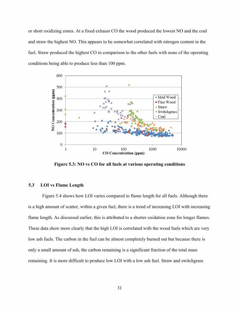
or short oxidizing zones. At a fixed exhaust CO the wood produced the lowest NO and the coal

and straw the highest NO. This appears to be somewhat correlated with nitrogen content in the

fuel. Straw produced the highest CO in comparison to the other fuels with none of the operating

conditions being able to produce less than 100 ppm.

Figure 5.3: NO vs CO for all fuels at various operating conditions

5.3 LOI vs Flame Length

Figure 5.4 shows how LOI varies compared to flame length for all fuels. Although there

is a high amount of scatter, within a given fuel, there is a trend of increasing LOI with increasing

flame length. As discussed earlier, this is attributed to a shorter oxidation zone for longer flames.

These data show more clearly that the high LOI is correlated with the wood fuels which are very

low ash fuels. The carbon in the fuel can be almost completely burned out but because there is

only a small amount of ash, the carbon remaining is a significant fraction of the total mass

remaining. It is more difficult to produce low LOI with a low ash fuel. Straw and switchgrass

32

have higher ash content and therefore lower LOI than wood but the larger particle size

contributes to higher LOI than coal which has both high ash content and small particle size.

Figure 5.4: LOI vs visual flame length for all fuels at various operating conditions

Lower LOI usually indicates higher burnout percentages. However Figure 5.5

demonstrates that straw and switchgrass have lower burnout in spite of their low LOI. This is

first due to the large ash content of these two fuels as discussed previously, as well as large

particles which take longer to burnout.

33

Figure 5.5: Burnout vs visual flame length for all fuels at various operating conditions

The coal and switchgrass data are shown on a finer scale for LOI in Figure 5.6. At this

scale, the switchgrass data do not appear to correlate well with flame length. In order to

investigate the lack of correlation with this fuel, Figure 5.7 identifies various operating

conditions used with switchgrass These include high and low swirl and holding secondary air

flow constant, “constant air,” versus holding the total oxygen flow constant, “constant O2”. The

figure shows that it is primarily the data for constant O2 flow rate that do not correlate with flame

length. For these data, the flow of secondary air is significantly reduced creating a poor mixing

between fuel and oxidizer which lengthens the flame but the oxygen concentration in the burnout

zone is significantly increased because nitrogen as a diluent has been reduced and the residence

time has increased because of a lower total volume flow rate. This higher O2 concentration and

longer residence time help reduce LOI.

34

Figure 5.6: LOI vs visual flame length for switchgrass and coal at various swirl values and oxygen addition levels with burner configuration 1S2L3L

Figure 5.7: LOI vs visual flame length for switchgrass data

In “Constant Air” experiments the secondary air flow was held constant while oxygen

enrichment levels varied. In this case the total flow rate is not changing dramatically and the

recirculation zone remains at approximately the same strength for each data point while oxygen

35

concentration of the secondary is increased. This method of changing flame length produced the

trade-off consistent with all of the other data. The trend is most clear for the Maximum Swirl

case while the Minimum Swirl data are more scattered. In the Minimum Swirl case the lowered

swirl causes the flame to extend almost the entire length of the reactor. Swirl has a stronger

influence on flame length than oxygen addition to the secondary air.

In “Constant O2” experiments total oxygen mass flow into the BFR was held constant.

Thus the secondary air flow decreased dramatically when pure oxygen was added to the

secondary. This decreases flow velocity and recirculation zone strength which reduced mixing

and created longer flames. It is these data for which LOI does not correlate with flame length.

Because the sum of oxygen in the air and pure oxygen is constant, the post flame O2

concentration is not changed significantly. One possible explanation for why LOI did not

increase with increased flame length is a longer residence time produced by lowered secondary

air flow.

5.4 NO vs Flame Length

Figure 5.8 shows how NO concentration varies with flame length for all fuels. The two

new fuels (switchgrass and coal) lie along a similar trend line to medium wood while straw

produces more NO for a given flame length than the other fuels. It is not clear why the straw has

higher NO for the same flame length but may be caused by higher fuel nitrogen.

36

Figure 5.8: NO vs visual flame length for all data at various operating conditions

5.5 Measurement Comparison

The accuracy of the model developed previously was evaluated for all of the data

including the two new fuels investigated in this work by comparing calculated flame length with

the visually measured flame lengths as shown in Figure 5.9. Proportionality constants, c1 and c2,

were found by a best fit to the data and are unique values for each fuel.

Two data points have been added from data collected by the University of Utah. “Utah

OFC” refers to a 50 kW, oxy-combustion case with no swirl [28]. “Utah L1500” refers to a 1.5

MW, air-fired cased with an estimated swirl of 1.2 [29]. Both cases used bituminous coal similar

to that used in the BYU experiments but coal property data were not available. and were fit

to the data for the L1500 case and then used for both the L1500 and OFC cases. The L-1500 is

an exact match because the constants were selected to make it fit but the OFC flame length is

surprisingly well predicted with these constants given that the two cases are so different in

burner size, swirl amount, and oxidizer setup.

37

Figure 5.9: Calculated flame length vs. visual flame length for all data by fuel

Most of the fuels follow a slope reasonably well predicted by Owen’s model but the slope

of the coal data are noticeably flatter than the other fuels. There are no combinations of c1 and c2

that produce a steeper slope. All of the fuels tested by Owen are biomass fuels with high ASTM

volatile fractions while the coal volatile fraction is significantly lower. Because the measured

flame length is related to the volatile fuel flame and not the total fuel it was thought that the

model might be more accurate if the volatile flow rate, not the total fuel flow rate, was used.

5.6 Volatiles Flame Length

The flame length model is based on calculating the distance from the burner where the

fuel oxidizer ratio is stoichiometric. The amount of fuel is therefore critical to determining the

flame location. For the original model produced by Owen [3]the total mass of the fuel including

volatiles and solid fractions was used. The flame however is actually located at the boundary

where the volatile fuel to oxidizer mixture is stoichiometric. A visible flame is produced by

38

radiating soot particles indicating the oxidation of gaseous fuel rich pyrolysis products. The

flame is expected to be located where the volatile fuel reacts, not the solid fuel. Using the

volatile fuel fraction is therefore more consistent with the visual measured flame value than

inclusion of the total fuel mass.

In order to correct for this shortcoming in the previous model, the mass flow term was

multiplied by the volatiles fraction ( ) obtained from the ASTM Proximate Analysis resulting in

Equation 5.1. While more complex models could be used to obtain the volatile fraction such as

the Coal Percolation and Devolatilization (CPD) Model [30] or FLASHCHAIN [31] the ASTM

results are readily available for most fuels and the fidelity is consistent with the rest of the model.

, ,

,

(5.1)

This model was again fit to experimental data to determine new values of c1 and c2 for

each fuel. Figure 5.10 shows the comparison of calculated and visual flame lengths with the

inclusion of the volatiles fraction in the model. Using the volatiles fuel flow clearly improves the

correlation of the coal but slightly increases the scatter in the biomass and Utah data. The values

of R2 were calculated for both the original (R2 = 0.7707) and this modified model (R2 = 0.7591)

and it was found that R2 decreased by 0.0116.

The model assumes that oxygen in the fuel carrier gas and the center tube are perfectly

mixed at the burner exit. Clearly this is not the case as it takes some distance for the two streams

to mix. For coal the volatile fraction is small and the amount of oxygen required to reach

stoichiometric is the lowest of all the fuels. This makes the perfectly mixed assumption less valid

and the model is less predictive. When the flow of pure oxygen in the center tube approaches

stoichiometric the model cannot be valid. For example, at 8 kg/hr the model predicts a very short

39

flame length of 0.2 m. This is approximately the length of 4 primary burner diameters which is

too short for the oxygen to mix with the fuel. Predicted values of 4 burner diameters or less

should not be considered valid and are not shown in Figure 5.10.

Figure 5.10: Calculated volatiles flame length vs. visual volatiles flame length for all data by fuel

5.7 Trends in Flame Length Suggested By Model Results

The model was used to understand trends in burner design variables by changing one

variable while holding all other variables constant. Some variables had little effect while others

were much more significant. Results were obtained for each fuel but only those for medium

wood are shown because of the larger number of experimental results available to compare with

the model.

40

5.7.1 Primary Fuel Tube Diameter

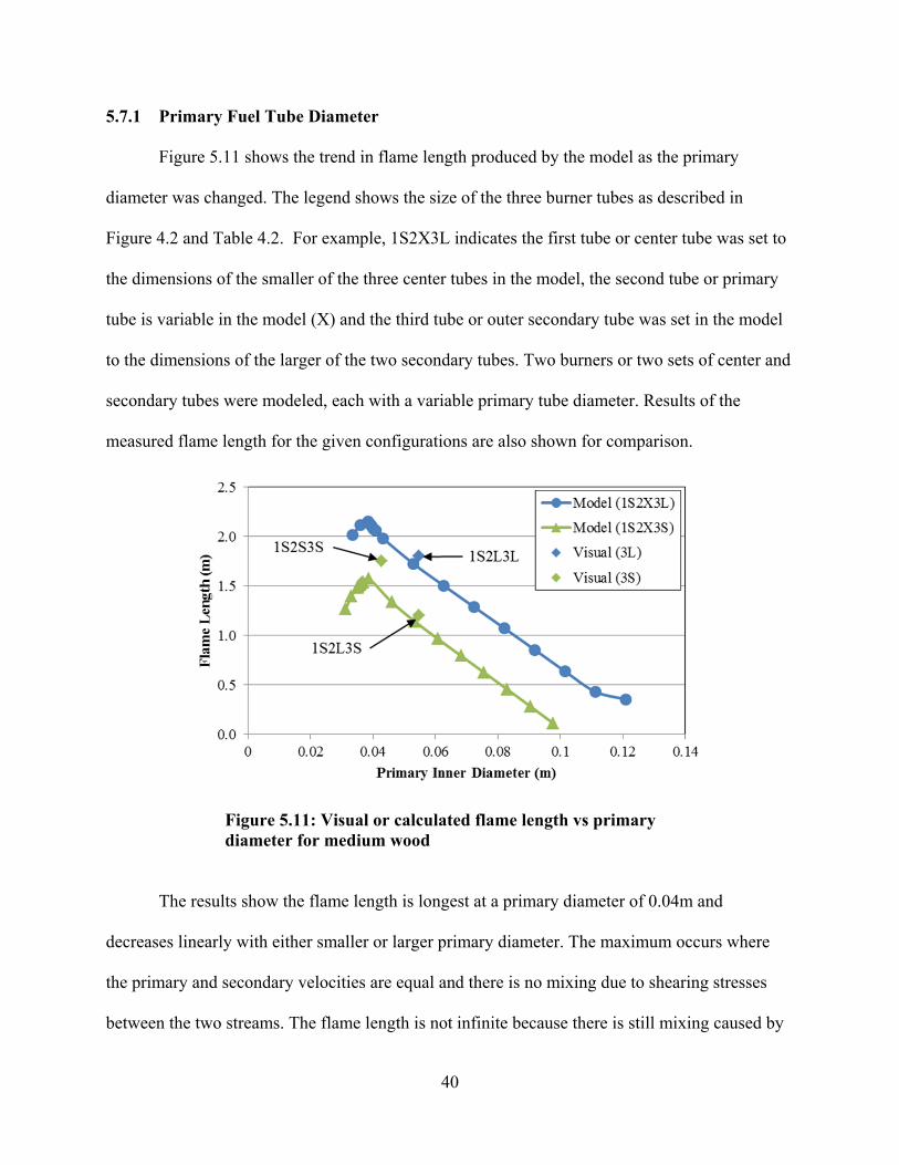
Figure 5.11 shows the trend in flame length produced by the model as the primary

diameter was changed. The legend shows the size of the three burner tubes as described in

Figure 4.2 and Table 4.2. For example, 1S2X3L indicates the first tube or center tube was set to

the dimensions of the smaller of the three center tubes in the model, the second tube or primary

tube is variable in the model (X) and the third tube or outer secondary tube was set in the model

to the dimensions of the larger of the two secondary tubes. Two burners or two sets of center and

secondary tubes were modeled, each with a variable primary tube diameter. Results of the

measured flame length for the given configurations are also shown for comparison.

Figure 5.11: Visual or calculated flame length vs primary diameter for medium wood

The results show the flame length is longest at a primary diameter of 0.04m and

decreases linearly with either smaller or larger primary diameter. The maximum occurs where

the primary and secondary velocities are equal and there is no mixing due to shearing stresses

between the two streams. The flame length is not infinite because there is still mixing caused by

41

recirculation as represented by the first term in the denominator of Equation 5.1. The triangle

marked 1S2L3L shows the measured flame length for that burner (1S2L3L) which is in good

agreement with the model.

The burner configuration with the smaller secondary diameter (3S) has shorter flame

lengths because the area between the primary and secondary tubes is smaller creating a higher

velocity for the secondary oxidizer and more swirl. Therefore the first term in the denominator of

Equation 5.1 is larger. The same trend is apparent in the model where the flame is longest at a

geometry which creates no velocity difference between the primary and secondary streams and

the flame gets shorter as that velocity difference increases. The diamond marked 1S2L3S is

shown to indicate the measured flame length which again agrees very well with the model. A

third measured data point is shown where both the primary and secondary diameters are the

smallest of the available hardware choices and this data point also agrees relatively well with the

model as it should fall along with the triangular data points.

5.7.2 Secondary Diameter

The next variable investigated was the diameter of the secondary oxidizer tube (D5,

Figure 4.2). As secondary diameter increases with a fixed primary diameter, secondary area

increases and secondary air velocity decreases reducing mixing between the two streams and

increasing flame length. Figure 5.12 shows a trend of increasing flame length with increasing

secondary diameter. As the secondary diameter increases from 0.07 to 0.24 m, the secondary air

velocity is getting closer to the primary air velocity and therefore both first term (swirl mixing)

and second term (shear flow mixing) in the denominator are getting smaller but the swirl

controlled mixing term is dominant and therefore the flame length continues to grow with

42

increasing secondary diameter. Two measured data points are shown in the figure, which are in

good agreement with both the magnitude and trend predicted by the model.

Figure 5.12: Visual or calculated flame length vs secondary diameter for medium wood

5.7.3 Primary Mass Flow

There are three ways to vary the primary mass flow: 1) Vary primary air flow, 2) vary

fuel mass flow, and 3) vary total primary flow while holding the fuel to air ratio in the stream

constant. Each of these is presented here.

Figure 5.13 shows the model predicts a slightly decreasing flame length with increasing

primary air mass flow rate. The result is a combination of increased air to fuel ratio increasing

favoring a shorter flame and increasing primary velocity to be closer to secondary flow velocity

causing increased flame length. The net effect is a slightly shorter flame with increasing primary

air flow rate.

43

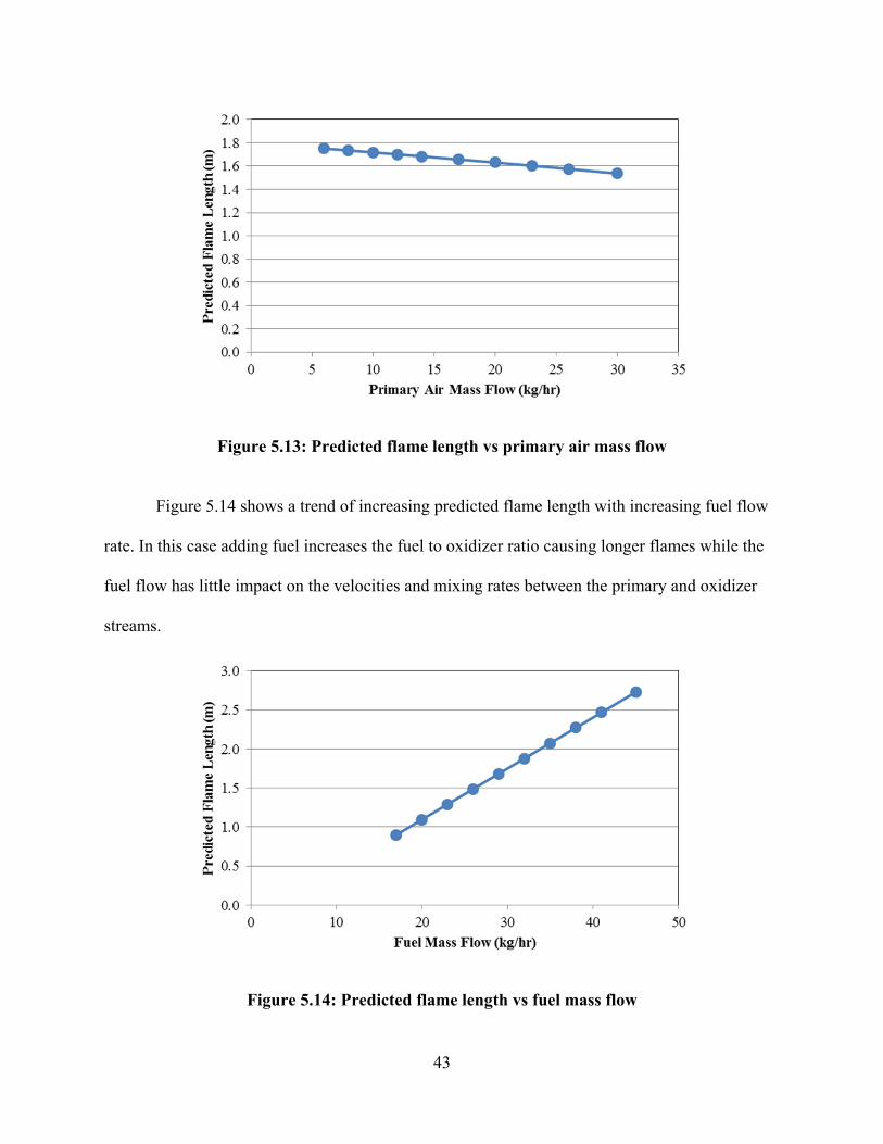
Figure 5.13: Predicted flame length vs primary air mass flow

Figure 5.14 shows a trend of increasing predicted flame length with increasing fuel flow

rate. In this case adding fuel increases the fuel to oxidizer ratio causing longer flames while the

fuel flow has little impact on the velocities and mixing rates between the primary and oxidizer

streams.

Figure 5.14: Predicted flame length vs fuel mass flow

44

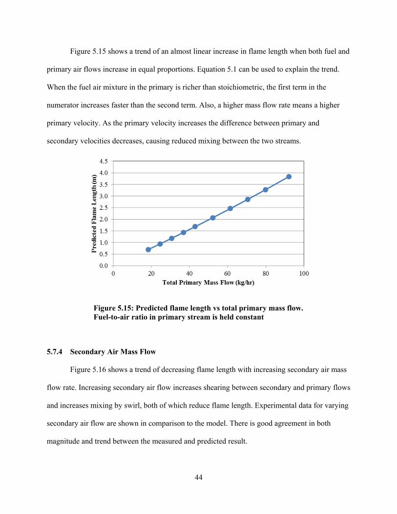
Figure 5.15 shows a trend of an almost linear increase in flame length when both fuel and

primary air flows increase in equal proportions. Equation 5.1 can be used to explain the trend.

When the fuel air mixture in the primary is richer than stoichiometric, the first term in the

numerator increases faster than the second term. Also, a higher mass flow rate means a higher

primary velocity. As the primary velocity increases the difference between primary and

secondary velocities decreases, causing reduced mixing between the two streams.

Figure 5.15: Predicted flame length vs total primary mass flow. Fuel-to-air ratio in primary stream is held constant

5.7.4 Secondary Air Mass Flow

Figure 5.16 shows a trend of decreasing flame length with increasing secondary air mass

flow rate. Increasing secondary air flow increases shearing between secondary and primary flows

and increases mixing by swirl, both of which reduce flame length. Experimental data for varying

secondary air flow are shown in comparison to the model. There is good agreement in both

magnitude and trend between the measured and predicted result.

45

Figure 5.16: Measured and predicted flame length vs secondary air mass flow

5.7.5 Oxygen Enrichment

Oxygen was added in two locations: 1) Premixed with the secondary air or 2) Center

injection. Figure 5.17 shows the trend produced by the model as the mass flow of enriching

oxygen premixed into the secondary air varies. The model agrees with the measurements that

there is a decrease in flame length with an increase in the amount of oxygen added to the

secondary air. The model predicts both the absolute value and the change in flame length

relatively well.

Figure 5.18 shows measured and modeled flame lengths with oxygen addition via the

center tube. The model predicts a 33% drop in flame length with the addition of 8 kg/hr of

oxygen. The data show a more moderate decrease on the order of 10%. The model assumes that

all of the oxygen from the center tube is immediately mixed with the incoming fuel while the

data suggest the oxygen takes time to mix and does not have as great an impact on flame length

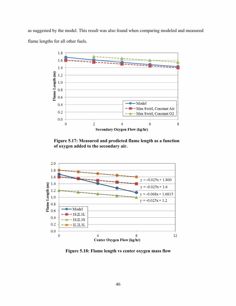
46

as suggested by the model. This result was also found when comparing modeled and measured

flame lengths for all other fuels.

Figure 5.17: Measured and predicted flame length as a function of oxygen added to the secondary air.

Figure 5.18: Flame length vs center oxygen mass flow

47

5.8 Predicting Empirical Constants

The model contains two empirical constants, c1 and c2, from a best fit for all of the data

points for a given fuel and given reactor/burner combination. While this is useful for determining

trends expected by changes in geometry, it was of interest to determine if a single set of

constants could be used for all fuels and burner/reactor combinations or if the constant could

somehow be determined without the need for experimental data. The values for c1 and c2 used in

the results shown in Figure 5.10 are shown in Table 5.1. It was observed that for three of the five

fuels, particularly those with smaller particles, c1 is equal to zero suggesting mixing due to swirl

is more important for these flames than mixing by shear. The data obtained for these flames did

not include zero swirl and therefore a finite value for c1 is needed to make the model more

generally applicable.

Table 5.1: Values of empirical constants for each fuel

c1 c2 Medium Wood 0.002851 0.021731 Straw 0 0.019396 Fine Wood 0 0.036819 Switchgrass 0.006844 0.012681 Coal 0 0.016059 U of U 0.00226 0.001947

Data taken in the oxyfuel combustor (OFC) at the University of Utah (U of U) without

swirl produced a c1 very close to the medium wood results in the BFR at BYU. Using this value

(0.00226) for c1 for all fuels new values for c2 were determined for c2 for each fuel as shown in

Table 5.2. A comparison of measured and predicted flame lengths for all fuels using these values

for c2 are shown in Figure 5.19. The difference between these results and those in Figure 5.10 are

48

insignificant. The small impact of c1 on the model is due to the fact that swirl is the dominant

mode for mixing for most of the data obtained in this work.

Table 5.2: Values of empirical constants using the same c1 for all fuels

c1 c2 Medium Wood 0.00226 0.022488 Straw 0.00226 0.015871 Fine Wood 0.00226 0.033449 Switchgrass 0.00226 0.018762 Coal 0.00226 0.012807 U of U 0.00226 0.001947

Figure 5.19: Calculated volatiles flame length vs visual volatiles flame length using a global constant c1 for all fuels with unique c2 for each fuel.

Values for c2 are plotted as a function of fuel diameter in Figure 5.20. Early data seemed

to suggest that c2 was a function of particle diameter indicating that flames with small particles

were more dependent on swirl induced mixing as the fine particles would follow the flow while

49

larger particles were more likely to penetrate a recirculation zone and mixing was controlled

more by shearing between fuel and air flows. This correlation did not hold for all of the data and

therefore an average value of c2 = 0.02 was selected as the best option for predicting flame

lengths when empirical data are not available.

Figure 5.20: c2 values vs average particle size for each fuel

Using c1=0.00226 and c2=0.02 for all fuels flame length was calculated and is compared

to visual flame length in Figure 5.21. These data show fuels are clumped together but are overall

more scattered than when the model constants can be determined by experimental results. The

fine wood flames are all predicted to be longer than the measured flames and almost all of the

straw flames are predicted to be shorter than the measured flames. The model predicted 90% of

the flame lengths to be within 38% of the measured value.

Two types of data are not within 50% of the predicted flame length: coal flames in the

BFR with center oxygen addition and the coal flame in the L1500. The reason for poor

prediction of the BFR with center oxygen addition is discussed in Section 5.7.5 but involves the

assumption that center oxygen addition is perfectly mixed at the burner exit.

50

The reason for a poor prediction of the L1500 flame length is not clear. This flame had

significantly higher primary air to fuel ratio and higher velocities than the BFR burner. The

physical size of the burner was only 50 – 100% larger than the BFR burner.

Figure 5.21: Calculated vs visual volatiles flame lengths with set values for both constants

5.9 Empirical Constants and the Stokes Number

A second method of predicting c1 and c2 explored in this work was to correlate their

values with the Stokes number. In a study by Probstle and Wenz [32] the response of a particle to

gas motion in a pulverized coal combustor was characterized by a “time constant” defined by

Equation 5.2 where ρp is the density of the particle, dp is the particle diameter, and μf is the

dynamic viscosity of the fluid. A characteristic time of the fluid can be found as the ratio of a

characteristic length of the fluid (lf) to the fluid velocity (uf ) as shown in Equation 5.3. The ratio

of the particle time constant, ,and the fluid characteristic time, , creates Equation 5.4 which

is often referred to as the Stokes number (Stk) and is a parameter that evaluates the tendency of a

solid particle to follow the streamlines of the fluid flow or the inertial trajectory of the particle.

51

For Stk≪ 1 the particle will follow the fluid flow streamlines and for Stk≫1 the particle will

follow its inertial trajectory.

18 (5.2)

(5.3)

18 (5.4)

Using an average velocity of the primary stream (Vp) for uf and the theoretical

recirculation zone diameter (b) for lf values for c1 and c2 were calculated for each fuel. Figure

5.22 and Figure 5.23 show these values and how they correlate with the Stokes number. c1

appears to increase with increasing Stokes number while c2 decreases with increasing Stokes

number. However the trends in c2 appear are offset for coal cases compared to biomass fuels.

This is likely due to the amount of volatiles in the two types of fuels. Biomass fuels have higher

volatile fractions which would require higher constants to acquire the correct flame length.

Figure 5.22: c1 vs Stokes number for each fuel

52

Figure 5.23: c2 vs Stokes number for each fuel

Using the equations shown in these figures positive values for c1 and c2 were calculated

and are shown in Table 5.3. The values of c1 for fine wood and coal were slightly negative by the

correlation but were set to zero. Using these values the model was once again compared to flame

length data as shown in Figure 5.24. Using these predicted values for c1 and c2 based on the

Stokes number of the particles, the model then predicted 90% of the flame lengths to be within

44% of the measured value.

Table 5.3: Values of c1 and c2 using the curve fit with Stokes number

c1 c2 Medium Wood 0.004423 0.014851

Straw 0.001929 0.024288

Fine Wood 0 0.033371

Switchgrass 0.003574 0.018062

Coal 0 0.016099

U of U 0.002572 0.001993

53

Figure 5.24: Calculated vs visual volatiles flame lengths with constants that are correlated with the Stokes number

5.10 Discussion

The agreement between measured and predicted flame lengths is surprisingly good for the

wide range of conditions measured. The model is based on mixing considerations for gaseous

flows and may capture effects related to particle trajectory when correlating c1 and c2 with the

Stokes number, but still does not account for the effects of devolatilization time and particle

heating rates. The data suggest that although these physical processes are important, fuel oxidizer

mixing is the dominant factor in determining flame lengths for fine particle flames as it is in

gaseous flames. Once a flame length has been established, the impact of a change in burner

geometry on a change in flame length can be qualitatively assessed by considering the impact

that change will have on mixing related to swirl and shearing. Oxygen addition directly into the

fuel stream will have a greater impact on flame length than oxygen in an adjacent stream. When

oxygen is added to a secondary stream, if the oxygen addition results in slower velocities and

less mixing, the flame length will increase in spite of the added oxygen. Very long flames can

54

be obtained by matching fuel and oxidizer flow velocities and reducing swirl which limits

mixing. This will also result in lifted unstable flames.

55

6 SUMMARY AND CONCLUSIONS Experimental data were taken using a swirled burner with three coaxial tubes for nearly

400 operating conditions. Data for two new fuels, switchgrass and coal, which included about

100 data points, were added to the previous 300 BYU data points for hardwoods and straw from

work done by Owen [3]. Data points consisted of varying swirl, fuel type, air flow rate, enhanced

oxygen flow rate and oxygen addition location. Trends in NO and LOI were shown to correlate

with flame length by Owen and data new to this work. Increasing flame length correlated with

decreasing NO and increasing LOI. The analytical model developed by Owen [3] was compared

to the current and previous flame length data.

The previous model did not predict changes in flame length when coal was used as the

fuel. An improved model was proposed that included the ASTM volatile fraction as the amount

of fuel entering the system instead of the total fuel mass flow. This improved the model’s ability

to predict trends in the length of coal flames while only changing the R2 value of non-coal flames

by less than 2%.

The model was used to explore trends involving the effect of burner geometries and

mass flow rates on flame length. For each variable investigated, all other variables were held

constant

56

1) Increasing primary tube diameter decreases flame length because the area of the

secondary flow (annulus between primary and secondary tube) decreases increasing the

secondary velocity and mixing between the two streams.

2) Increasing secondary tube diameter produces longer flames because the area of the

secondary oxidizer is increased and the flow velocity decreases reducing mixing between

fuel and oxidizer and decreasing swirl,

3) Increasing primary air flow produces shorter flames because oxidizer is added to the fuel

stream.

4) Increasing fuel flow produces longer flames because more oxidizer mixing into the fuel

stream is required to reach a stoichiometric mixture

5) Increasing secondary air flow produces shorter flames because it increases secondary

oxidizer velocity and swirl increasing mixing between fuel and oxidizer.

6) Increasing oxygen flow in the secondary stream produces slightly shorter flames as the

velocity is not greatly increased but the concentration of oxygen increases mixing of

oxidizer into the fuel rich center.

7) Increasing oxygen flow in the center tube produces significantly shorter flames as the

oxygen is added directly to the fuel rich center jet and decreases the oxygen required to

mix the fuel to a stoichiometric mixture.

Two methods were investigated to determine constants that could be used with the model

without additional empirical data. The first method looked at using a constant c1 and c2 for all

fuels. The results showed that the model predicted 90% of the flame lengths within ±38% of the

measured value.

57

The second method attempted to correlate c1 and c2 with the Stokes number. This

technique allows the particle size to become a part of the flame length correlation. The c1 results

were found to correlate reasonably well with the Stokes number for all fuels while the c2 data

were correlated by the Stokes number within a given fuel type, coal or biomass. Biomass fuels

have high volatile fractions and produced higher c2 values than coal which is a lower volatile

fuel. Using a single linear correlation for c1 and separate linear correlations for c2 for coal and

biomass 90% of the predicted flame lengths were within 44% of the measured values.

58

REFERENCES

[1] C. A. T. Center, "Nitrogen Oxides (NOx), Why and How They Are Controlled," EPA, 1999.

[2] "Clean Air Act Overview," EPA, 30 March 2016. [Online]. Available: https://www.epa.gov/clean-air-act-overview/clean-air-act-text. [Accessed 11 November 2016].

[3] S. Owen, Burnout, NO, and Flame Characterization from an Oxygen-Enriched Biomass Flame, Provo: Brigham Young University, 2015.

[4] S. Azuhata, K. Narato, H. Kobayashi, N. Arashi, S. Morita and T. Masai, "A Study of Gas Composition Profiles for Low NOx Pulverized Coal Combustion and Burner Scale-up," in Twenty-first Symposium (International) on Combustion/The Combustion Institute, 1986.

[5] M. L. Holtmeyer, G. Li, B. M. Kumfer, S. Li and R. L. Axelbaum, "The Impact of Biomass Cofiring on Volatile Flame Length," Energy & Fuels, vol. 27, pp. 7762-7771, 2013.

[6] S. P. Burke and T. E. W. Schumann, "Diffusion Flames," Industrial and Engineering Chemistry, vol. 20, no. 10, pp. 998-1004, 1928.

[7] F. G. Roper, "The Prediction of Laminar Jet Diffusion Flame Sizes: Part I. Theoretical Model," Combustion and Flame, vol. 29, pp. 219-226, 1977.

[8] F. G. Roper, "The Prediction of Laminar Jet Diffusion Flame Sizes: Part II. Experimental Verification," Combustion and Flame, vol. 29, pp. 227-234, 1977.

[9] S. R. Turns, "Laminar Diffusion Flames," in An Introduction to Combustion Concepts and Applications, New York, McGraw Hill Education, 2014, pp. 311-365.

[10] J. A. Fay, "The Distributions of Concentration and Temperature in a Laminar Jet Diffusion Flame," Journal of Aeronautical Sciences, vol. 21, pp. 681-689, 1954.

[11] S. R. Turns, "Turbulent Nonpremixed Flames," in An Introduction to Combustion Concepts and Applications, New York, McGraw Hill Education, 2014, pp. 486-526.

59

[12] K. Wohl, C. Gazley and N. Kapp, "Diffusion Flames," in Third Symposium on Combustion and Flame and Explosion Phenomena, Baltimore, 1949.

[13] M. A. Delichatsios, "Transition from Momentum to Buoyancy-Controlled Turbulent Jet Diffusion Flames and Flame Height Relationships," Combustion and Flame, vol. 92, pp. 349-364, 1993.

[14] H. A. Becker and D. Liang, "Visible Length of Vertical Free Turbulent Diffusion Flames," Combustion and Flame, vol. 32, pp. 115-137, 1978.

[15] Y. Kang, T. Lu, X. Lu, X. Gou, X. Huang, S. Peng, X. Ji, Y. Zhou and Y. Song, "On Predicting the Length, Width, and Volume of the Jet Diffusion Flame," Applied Thermal Engineering, vol. 94, pp. 799-812, 2016.

[16] M. Hupa, "International Flame Research Foundation," 24 January 2006. [Online]. Available: http://www.ffrc.fi/Liekkipaiva_2006/Liekkipaiva2006_IFRF_Today_HUPA.pdf. [Accessed 10 November 2016].

[17] R.-H. Chen and J. F. Driscoll, "The Role of the Recirculation Vortex in Improving Fuel-Air Mixing within Swirling Flames," in Twenty-Second Symposium (International) on Combustion/The Combustion Institue, 1988.

[18] K. L. Smith, L. D. Smoot, T. H. Fletcher and R. J. Pugmire, "Devolatilization Rate Processes and Products," in The Structure and Reaction Processes of Coal, New York, Plenum Press, 1994, pp. 209-321.

[19] K. L. Smith, L. D. Smoot, T. H. Fletcher and R. J. Pugmire, "Char Oxidation, Conversion, and Reaction Rate Processes," in The Structure and Reaction Processes of Coal, New York, Plenum Press, 1994, pp. 325-404.

[20] K. L. Smith, L. D. Smoot, T. H. Fletcher and R. J. Pugmire, "Geochemistry and Macromolecular Structure of Coal," in The Structure and Reaction Processes of Coal, New York, Plenum Press, 1994, pp. 37-75.

[21] S. R. Turns, "Burning of Solids," in An Introduction to Combustion Concepts and Applications, New York, McGraw Hill Education, 2014, pp. 527-555.

[22] T. Chae, "Numerical simulations of a large scale oxy-coal burner," in Cleaner Combustion and Sustainable World, Springer-Verlag Berlin Heidelberg and Tsinghua University Press, 2012, pp. 643-645.

[23] L. Chen and A. F. Ghoniem, "Simulation of Oxy-Coal Combustion in a 100 kWth Test Facility Using RANS and LES: A Validation Study," Energy & Fuels, vol. 26, pp. 4783-4798, 2012.

60

[24] J.-D. Kim, G.-B. Kim, Y.-J. Chang, J.-H. Song and C.-H. Jeon, "Examination of Flame Length for Burning Pulverized Coal in Laminar Flow Reactor," Journal of Mechanical Science and Technology, vol. 24, no. 12, pp. 2567-2575, 2010.

[25] S. R. Turns, An Introduction to Combustion Concepts and Applications, New York: McGraw Hill Education, 2014.

[26] J. D. Thornock, "Burnout, NO, Flame Temperature, and Radiant Intensity from Oxygen-Enriched Combustion of a Hardwood Biomass," Brigham Young University, Provo, 2013.

[27] E. G. Eddings, "Institute for Clean and Secure Energy - Experimental Facilities," University of Utah, 2015. [Online]. Available: http://www.icse.utah.edu/experimental_facilities. [Accessed 13 March 2017].

[28] J. Zhang, K. Kelly, E. G. Eddings and J. Wendt, "OXY-coal combustion: Effects of PO2 on coal jet stability in O2/CO2 environments," 25th Annual International Pittsburgh Coal Conference, PCC - Proceedings, 2008.

[29] A. Fry, Interviewee, Personal Communication. [Interview]. 9 August 2016.

[30] T. Fletcher, A. Kerstein, R. Pugmire, M. Solum and D. Grant, "A Chemical Percolation Model For Devolatilization: Summary," University of Utah, Salt Lake City.

[31] S. Niksa and A. Kerstein, "FLASHCHAIN Theory for Rapid Coal Devolatilization Kinetics. 1. Formulation," Energy & Fuels, no. 5, pp. 647-665, 1991.

[32] G. Probstle and W. Wenz, "Velocity Measurements in a Swirl Driven Pulverized Coal Combustion Chamber," Combustion and Flame, vol. 72, pp. 193-203, 1988.

61

APPENDIX A LOSS ON IGNITION (LOI) PROCEDURE

Loss on ignition was determined using the procedure outlined below. Small1.3 ml

crucibles were used so that a minimal amount of ash would be required and so that three

replications for each operating condition could be obtained from the ash collected.

1. Weigh empty ceramic crucibles (This weight will need to be subtracted from other weights measured in Steps 2, 4, and 6 for the actual weight of the ash)

2. Fill crucibles with ash to about ¾ maximum capacity to prevent spillage and weigh again 3. Heat sample in conventional oven at 105°C for 4 hours to remove moisture 4. Weigh crucibles for moisture free ash weight,

5. Heat sample in conventional oven at 750°C for 6-8 hours 6. Weigh crucibles for carbon free ash,

7. Calculate LOI using the following equation:

(A.1)

8. Carbon burnout may be calculated using the following equation where is the ash content from ASTM proximate analysis

%1

1 ∗ 1 (A.2)

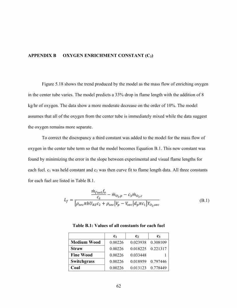
62

APPENDIX B OXYGEN ENRICHMENT CONSTANT (C3)

Figure 5.18 shows the trend produced by the model as the mass flow of enriching oxygen

in the center tube varies. The model predicts a 33% drop in flame length with the addition of 8

kg/hr of oxygen. The data show a more moderate decrease on the order of 10%. The model

assumes that all of the oxygen from the center tube is immediately mixed while the data suggest

the oxygen remains more separate.

To correct the discrepancy a third constant was added to the model for the mass flow of

oxygen in the center tube term so that the model becomes Equation B.1. This new constant was

found by minimizing the error in the slope between experimental and visual flame lengths for

each fuel. c1 was held constant and c2 was then curve fit to flame length data. All three constants

for each fuel are listed in Table B.1.

, ,

, (B.1)

Table B.1: Values of all constants for each fuel

c1 c2 c3 Medium Wood 0.00226 0.023938 0.308109

Straw 0.00226 0.018225 0.221317

Fine Wood 0.00226 0.033448 1

Switchgrass 0.00226 0.018959 0.797446

Coal 0.00226 0.013123 0.778449

63

In Figure B.1 this refined version of the flame length model is compared to experimental

data. The new constant appears to slightly reduce the overall error. Unfortunately there currently

does not appear to be any physical explanation for this constant.

Figure B.1: Calculated flame length (m) with a third proportionality constant vs visual volatiles flame length