Embed Size (px)
Citation preview
Physica 133A (1985) 1.52-172
North-Holland, Amsterdam
AN ANALYTICAL MODEL OF TRACER DIFFUSIVITY
IN COLLOID SUSPENSIONS
R.B. JONES and G.S. BURFIELD
Department of Physics, Queen Man C’ollege. M11e End Road, London El 4NS. LJK
Received 21 February 19X5
We present an analytical mode1 of the tracer diffusivity of a colloid particle applicable to a
suspension at a density low enough that only pair interactions of the particles need be considered.
We assume a pair potential consisting of an infinitely repulsive hard core together with an attractive short range tail as well as hydrodynamic pair interactions which are described by the
general mobility series of Schmitz and Felderhof which allow differing hydrodynamic boundary
conditions. Using our earlier low density expansion of the generalized Smoluchowski equation we
obtain an expression for the tracer diffusivity identical to that obtained by Batchelor from a
different derivation. For a class of simple analytic potential functions we show how the tracer
diffusivity may be evaluated by quadratures. We present explicit high order mobility seriec for both
stick and slip hydrodynamic boundary conditions and we use these to evaluate the tracer diffusivity numerically for a range of hard core radii. We distinguish short time and long time components of
the tracer diffusivity and show that the relative magnitude of these components is quite sensitive to the hydrodynamic boundary conditions.
1. Introduction
An interesting set of problems in colloid science concern the ditfusivities
which may be studied in a suspension. In a monodisperse suspension one may
consider the collective diffusivity or the self-diffusivity of a tagged tracer
particle while in a polydisperse suspension one may consider diffusivities for
each of the component species. More generally one can introduce wave vector-
and frequency-dependent diffusivities which can be studied by dynamic light
scattering measurements’-“). All of these diffusivities are of interest because
they depend upon the interactions among the colloid particles and thus give
information about the interparticle forces. In the present paper we study a
model of the tracer particle diffusivity D’ for a suspension of identical
spherically symmetric particles which interact by two-body potentials as well as
by hydrodynamic forces. We assume that the potentials are short ranged and
that the suspension is sufficiently dilute that only pair interactions need be
037%4371/85/$03.30 @ Elsevier Science Publishers B.V.
(North-Holland Physics Publishing Division)

TRACER DIFFUSIVI-IY IN COLLOID SUSPENSIONS 153
considered. Our model is one in which both the potential and hydrodynamic
interactions can be varied and in which an expression for the tracer diffusivity
can be given in closed analytic form so that numerical evaluation is straight-
forward.
Batchelo?‘) has presented accurate numerical results for polydisperse sus-
pensions with variable two body potentials but with a fixed model of the
hydrodynamic interactions. Our model complements his work in that we study
the result of changing the hydrodynamic boundary conditions as well as the
potential interactions and our numerical procedure is different in nature from his.
It is of interest that we arrive at an expression for the self-diffusivity which can be
identified precisely with Batchelor’s result6) although our respective derivations
have quite different starting points.
In section 2 we review different definitions of the tracer diffusivity indicating
how one can distinguish “short time” and “long time” contributions to it. In
section 3 we describe the class of two body potentials considered and we
present accurate high order series expansions of the mobility functions for two
different hydrodynamic models. In section 4 we specialize the results of earlier
work8,9) to give analytic expressions for the “short time” and “long time”
contributions to DT. In sections 5 and 6 we show how one can use our model
potential together with the mobility series to reduce the problem of calculating
DT to simple quadratures. Several key steps in the numerical work depend on
the use of a computer system which can perform algebraic manipulations. In
section 7 we present selected numerical results and indicate the connection
between our derivation and that of Batchelor.
2. Definition of diffusivities
In this paper we discuss the tracer diffusivity of a tagged particle which could
be measured in a diffusion experiment in which the tagged particle moves
through a macroscopic concentration gradient of untagged particles. For sim-
plicity we regard the tagged particle as being identical to the untagged particles
in every respect except for its carrying a label which experimentally might be
an index of refraction different from that of the other particles. The case when
the tagged particle differs in size or interactions from the untagged particles is
easily included in our general method but would greatly complicate the details
of the discussion. In order to compare our formalism with previous work we
first consider different methods of defining a tracer diffusivity.
One simple approach is to obtain the tracer particle diffusivity as the limit of
one of the diffusivities appropriate to a polydisperse suspension of many
species. Thus consider a suspension of spherically symmetric particles of m

1.54 R.B. JONES AND G.S. BURFIELD
different species with the ith species characterized by a number density n’(r, t).
One may then introduce diffusivities D, associated with macroscopic concen-
tration gradients through a generalization of Fick’s law as6,“‘,“)
J,=-2 Dip-h”, p=l
(2.1)
where J, is the flux density of particles of species i. The coefficients D,, depend
upon the equilibrium volume fractions 4’ of the different species, 4’ =
ni4rR:/3, with nh = N’/V, and where N’ is the total number of particles of
species i, V is the volume of the suspension and R, is the radius of a particle of
species i. At low enough densities for suspensions with short range forces the
D,, can be expressed in first order virial expansion as’.“.“)
D,, = D’l4’TiJ (i f i), (2.2)
where Dp = Dfl with 0: the scalar diffusivity of a particle of species i in the
infinite dilution limit and the y,, ri, depend upon the particle interactions. The
scalar tracer diffusivity DT can be obtained from this polydisperse formalism by
considering the tracer particle to constitute a species of zero volume fraction
while all other particles constitute a second species of volume fraction 4 =
n,4rR3/3 where n,, = N/V with N the total particle number for the suspension,
DT = D”(1 + yT~). (2.3)
Light scattering studies of suspensions however require a more general
definition of diffusivities. In these experiments’) one can probe density fluctua-
tions which are space- and time-dependent and characterized by finite wave
number k and frequency w. By linear response methods2.“) one can introduce a
generalized self-diffusivity kernel D,(k, ) w such that DT is the value of D5 in the
hydrodynamic limit
DT = lii ljz D&k, w) . (2.4)
The derivation of the dynamical quantity D,(k, w) shows that it can be split into
two parts,
(2.5)

TRACER DIFFUSIVITY IN COLLOID SUSPENSIONS 155
where the “first cumulant” D:(k) represents an instantaneous response of the
tagged particle to a fixed environment of untagged particles while the “memory
function” M,(k, w) represents the contribution to D,(k, w) arising from the
dynamical evolution of this environment. In dynamic light scattering studies’)
these two components are known as “short time” and “long time” con-
tributions and under appropriate experimental conditions13.14) can be separately
measured. A macroscopic diffusion experiment however is unable to dis-
tinguish these components separately and gives only their combined con-
tribution to DT.
Some earlier attempts to calculate DT for hard spheres”.‘*) inadvertently
omitted the “long time” contribution but more recent workk9) has shown how
to correctly incorporate both contributions. The derivation by Batchelor rests
upon ideas of irreversible thermodynamics while our earlier treatment’) applies
statistical mechanical methods to a microscopic dynamical description of the
suspension by means of the generalized Smoluchowski equation (GSE)“). In
the present paper we will use the general formalism of our earlier work’) where
we computed D:(k) and M,(k, w) to first order in number density in the
hydrodynamical limit (2.4). We will be able to indicate the precise cor-
respondence between our final expression for DT and that given by Batchelor6)
from a different line of argument. For this purpose we will explicitly split yT
into a “short time” component yTS arising from D:(k) and a “long time”
component yTL arising from M,(k, w), so we will write eq. (2.3) as
D= = D”(l + yT4) = D”(l + (yTS + yTL)4).
In subsequent sections we quote analytical expressions for yTS and yTL and we
evaluate them numerically for differing models of the particle interactions.
3. Particle interaction model
For a sufficiently dilute suspension we need consider only pair interactions
which are of two sorts, direct potential interactions and hydrodynamic inter-
actions. The potential interactions are electrodynamic in origin and in principle
involve many body effects but for moderately dense suspensions there is a
widely used effective two-body potential16) which combines a strongly repul-
sive short range core with a longer range tail representing the combined
effects of screened Coulomb repulsion and attractive Van der Waals forces. For
numerical studies in the present article we crudely represent this effective
interaction by a two-body potential with an infinite repulsive hard core at an
interparticle separation r = 2R,, and outside the core a weak short range

156 R.B. JONES AND G.S. BURFIELD
attractive potential. We write it as
b(r) = += , r<2R,,
n
-NE 1
i ) r>2R,, r
(3.1)
where p = l/k,T, with k, Boltzmann’s constant and T the absolute tem-
perature, R is the structural or hydrodynamic radius of the particles (RP > R)
and for simplicity of computation n is an integer such that n 34. Our
numerical method can also deal with a potential which is a general polynomial
in (R/r) but we will use (3.1) for the illustrative numerical studies presented
later.
The hydrodynamic pair interactions”-“) are mediated by the suspending
fluid which is treated as a Newtonian fluid of shear viscosity 7~ described by
creeping motion hydrodynamics’“). The strength of these forces depends on the
boundary interaction of the colloid particle with the surrounding fluid. The
simplest model is to treat the particles as hard spheres (radius R) with stick
fluid boundary conditions at the surface. However for suspensions stabilized by
so-called steric forceslh) there is a coating of the colloid particles consisting of
long molecules which extend into the surrounding fluid so that the simple stick
boundary condition model may not be appropriate. Other fluid interaction
models could employ slip boundary conditions or could treat the particles as
being partly permeable. The strength of the hydrodynamic forces is expressed
through certain mobility functions. At moderate particle separations the
mobility functions may be expanded in series in powers of (R/r) while for very
close approach the series converge slowly and asymptotic expressions must be
used instead. The mobilities are known with high accuracy for all separations
only in the stick boundary condition model’“). However, the series represen-
tation has been derived for any boundary condition in a genera1 form by
Schmitz and Felderhof”.“). Because the hard core repulsion in our model
potential (3.1) prevents extremely close encounters and also because our
numerical technique exploits the nature of the series expansions we have used
the genera1 expressions of Schmitz and Felderhof to evaluate the mobilities in
series through terms of order (R/r)*“. In consequence we are able to study the
effect on yT of altering the boundary condition as well as the potential u(r). To summarize the mobility information’7a’8) we consider two freely rotating
identical spherical particles 1 and 2 acted on by forces F,, F2 respectively which
produce particle velocities Us, u2 related to the forces by
ul= CL:, - F, + p:: * F2 ,
u2 = pi, - F, + py2 - F, . (3.2)

TRACER DIFFUSIVITY IN COLLOID SUSPENSIONS 157
If r denotes the separation of centres of the two particles then the mobility
tensors pi can be expressed in terms of scalar functions a;(r), pi(r) as
(3.3)
Schmitz and Felderhof’7V’s) h ave provided an elegant general expression for
(Y:;, fi:j which enables one to calculate their series expansions to all orders in
(R/r). These general expressions which are given as eqs. (5.6) and (5.7) of their
third paper”) are correct but the evaluation which they give through order
(R/r)” in eqs. (6.1), (6.2) and (6.12) is not correct. We have ascertained this by
use of the symbolic manipulation package MACSYMA to carry out the
algebraic expansion of their eqs. (5.6) and (5.7) through order (R/r)“. By
specializing to stick boundary conditions we were then able to check these
expansions for the coefficients (Y::, (.y:: against the expansion (again performed
using MACSYMA) of the same coefficients derived from the exact solution to
the two sphere problem due to Brenne?).
We may write the form of the series expansions required in the following
way, where we introduce the variable z = Rlr with R the radius of each of the
two particles involved in the interaction:
m
4~Ra~,(z) = 2 ayz*“, n=O
(3.4)
47r~RP;r(z) = c b;.z*“, n=O
cc
47rvRP::(z) = c b;‘z”‘+‘. n=O
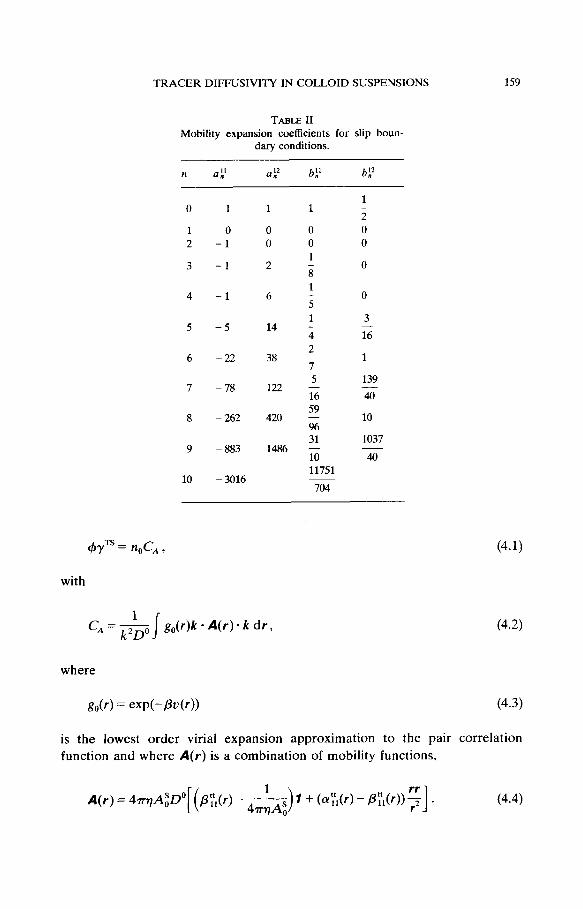
We have calculated all terms in these series through zzo for both stick and slip
boundary conditions at the particle surfaces. The relevant expansion
coefficients a:, bz are listed in tables I and II. For the most general models of
the hydrodynamic interaction between a particle and the fluid a set of scatter-
ing coefficients measures the strength of each multipole coupling’8). We have
the expansion of the mobilities through order zzo for general scattering
coefficients stored as a LISP file in the MACSYMA system; if anyone has need
of such expressions they are available on request from one of the authors
(RBJ). The dilute limit diffusion coefficient Do introduced in section 2 is

158 R.B. JONES AND G.S. BURFIELD
TABLE I
Mobility expansion coefficients for stick boundary conditions
2 0
3
1 0
5 2
2 11
3 3
4 7
167 5
3 883
6 12
7 102
795 8
8
9 ~ 1141
18683 10 -
8
2
3
0
25
2
-5
131
L
341
3 915 -
1;7
x 8567
4
0
17
24 5
6 23
8 31
I
2 1
i
0
0
0
1X9
64 1439
3 96
689 4201
24 114497
1536 10715
48 77179
80 3313
24 152227
480
96
expressible in terms of one of these scattering coefficients, Ai, as
Do- kBT 45-7A; ’
(3.5)
where AZ is equal to 3R/2 for stick boundary conditions and to R for slip
boundary conditions.
4. Short time and long time contributions
In this section we present analytical expressions for yTS and yTL based on the
general formulae derived by us in an earlier paper’). The short time con-
tribution was given earlier by one of us”) in a form which we can write as
TRACER DIFFUSIVITY IN COLLOID SUSPENSIONS 159
cbrn = n,c* 2
with
TABLE II Mobility expansion coefficients for slip boun-
dary conditions.
n at’ aA b” ” b’* n
4
5
6
1 1
0 0 -1 0
-1 2
-1 6
-5 14
- 22 38
- 78 122
- 262 420
- 883 1486
- 3016
1 1
z 0 0 0 0 1 8 0
1 ; 0
1 3
4 16 2 ? 1
5 139 - 16 40 59
10 96 31 1037
lo 40 11751
c, = - k2Do
g,(r)k . A(r) * k dr ,
704
(4.1)
(4.2)
where
go(r) = exp(-W(r)) (4.3)
is the lowest order virial expansion approximation to the pair correlation
function and where A(r) is a combination of mobility functions,
A(r) = 4wA;D”[ (P;,(r) - &) I+ (a::(r) - L%(r)) F] . (4.4)
160 R.B. JONES AND G.S. BURFIELD
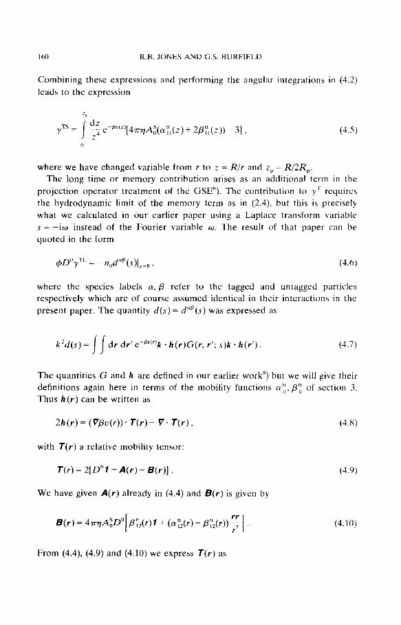
Combining these expressions and performing the angular integrations in (4.2)
leads to the expression
Ts- Y - I s e~P”“)[47i&(~~1(z) + 2/?:,(z)) - 3) ,
z (4.5)
where we have changed variable from r to z = R/r and zP = R/2R,.
The long time or memory contribution arises as an additional term in the
projection operator treatment of the GSE8). The contribution to yT requires
the hydrodynamic limit of the memory term as in (2.4) but this is precisely
what we calculated in our earlier paper using a Laplace transform variable
s = -iw instead of the Fourier variable w. The result of that paper can be
quoted in the form
c#dl”yTL = -nod”qS)ls=“, (4.6)
where the species labels (Y, ,f3 refer to the tagged and untagged particles
respectively which are of course assumed identical in their interactions in the
present paper. The quantity d(s) = d”“(s) was expressed as
k2d(s) = j j dr dr'em"""'k * h(r)G(r, r’; .~)k - h(r)). (4.7)
The quantities G and h are defined in our earlier work’) but we will give their
definitions again here in terms of the mobility functions N::, p:; of section 3.
Thus h(r) can be written as
2h(r) = (V@(r))- T(r)- V- T(r), (4.8)
with T(r) a relative mobility tensor:
T(r) = 2[0”7 + A(r) - B(r)] . (4.9)
We have given A(r) already in (4.4) and B(r) is given by
B(r) = 4qA$“[P?z(r)f + (a;;(r)-P::(r))F] . (4.10)
From (4.4) (4.9) and (4.10) we express T(r) as

TRACER DIFFUSIVITY IN COLLOID SUSPENSIONS 161
with
a(r) = 4mA&:‘,(r) - aY2(r)),
b(r) = 4wA%$(r) - &‘2(rN .
(4.11)
(4.12)
The quantity h(r) is written finally as
eSu(‘)r
h(r) = -c(r) - r ’
(4.13)
da(r) + 2(a(r) - b(r)) -
dr
+ a(r) cl t?“(‘) r I dr ’
The kernel G(r, r’; s) is a propagator describing the relative diffusion of a
pair of particles; it is a solution of the Green function equation*)
[S - e’“(‘) v- e-B”“‘T(r) * VjG(r, r’; s) = 6(r - r’), (4.14)
subject to the boundary conditions that the radial component of the relative
particle flux vanishes when the hard cores touch
r * T(r) - VG(r, r’; s) = 0, r = 2R,, (4.15)
and that G itself vanishes as r+ 00. The boundary conditions on G are
explained more fully in the appendix. As shown earlier’) we may expand G in
spherical harmonics and use the form of /z(r) to evaluate the angular integrals
in (4.7) leading to
d(s) = ($)’ j r2 dr / rr2 dr’ c(r)A,(r, r’; s) eP”“‘)c(r’), (4.16)
2R 2R
where A,(r, r’; s) is the only contribution from the harmonic expansion of G to
survive the angular integrations. To obtain y” then we need d(s) at s = 0 and
hence A,(r, r’; 0). The differential equation for A,(r, r’; 0) which follows from
the harmonic expansion of (4.14) is

162 R.B. JONES AND G.S. BURFIELD
= - X37D”r2a(r) 6(r - r’) (4.17)
The boundary conditions on A,(r, r’; 0) are that it vanishes as r+ = and, from
(4.19, that at r = 2R,
a(r)+$=O. (4.18)
Finally, we recall a reciprocity relation which G and A, each satisfy’).
empocr)A,(r, r’, s) = empI.““‘A1(r’, r; s), (4.19)
and which is helpful in simplifying the integrations in (4.16).
5. Construction of the kernel A,( r, r’; 0)
In this section we describe a method of solving eq. (4.17) for A,(r, r’; 0) which
depends upon two features of the interaction model described in section 3,
namely that the mobility functions a(r), b(r) are known to high order as series
in the variable z = R/r and that the potential /3u(r) is a polynomial in z. These
features enable us to construct A, explicitly by use of two independent
solutions to the homogeneous form of (4.17) which are obtained by the method
of Frobenius*‘). Throughout this section we express all functions of r as
functions of z = R/r.
The first requirement is to obtain two independent solutions to the homo-
geneous version of eq. (4.17), one of which is regular at z = 0 (r = 3~) the other
singular at this point. In terms of the variable z we write (4.17) as
d24 + f’(z) d4 / Q(z)4 3
dz2 z dz zZ &rD”Ra(z) qz - z’) ,
with P(z), Q(z) given as
P(z)= z 1 da(z) dpv(z)
____-___ a(z) dz I dz *
(5.1)
(5.2)

TRACER DIFFUSIVITY IN COLLOID SUSPENSIONS 163
20) Q(z)= -a(z). (5.3)
For our model potentials /?u(z) both P(z) and Q(z) are regular at z = 0 so we
express them in series form as
P(z) = 2 pnzn+l ) Q(z)= 2 q,,z". (5.4) n=O n=O
The indicial equation for the homogeneous form of (5.1) has two integer
roots, 2 and -1. However, if @(z) has no power of z of degree lower than .z4,
then the coefficients in the series expansions of a(z), b(z) are such (for both
stick and slip boundary conditions) that the second solution corresponding to
the root -1 does not have a logarithmic singularity at z = 0. If v(z) has terms
in z, z2 or z3 then such logarithmic terms are present, but for the present study
we have restricted /?v(z) so that the simpler case holds. We thus can find two
independent solutions fr(z), fz(z),
f,(z) = c ffizn+2 3
n=O
f2(z) = i + i: f’,z”_’ . n=3
(5.5)
The coefficients fi,fi are found by recursion formulae in terms of the
coefficients p,, q, in (5.4)
f+ -
k(k _ 3) - & 5 [@ - l)Pk-l-m + qk-,lf ,i > ka4. (5.6) m 3
The evaluation of the f: begins at k = 1 using as input f:, = 1 while for the f: one begins at k = 4 using as input fz = -1 for stick boundary conditions and
f: = 0 for slip boundary conditions. The detailed mobility series given in (3.4)
and tables I and II enable us to compute the f:, fi explicitly through k = 20.
The two independent solutions f,(z), f*(z) are
Wronskian has the simple form (f’(z) = df(z)/dz)
normalized so that their
(5.7)

164 R.B. JONES AND G.S. BURFIELD
For the model interactions of this paper we can now express A,(z, z'; 0)
explicitly in terms of ft(z),fJz). We can do this because the hard core
repulsion prevents any two particles from touching at separation r = 2R. If two
spherical particles do touch at this separation (z = f) then for both stick and
slip boundary conditions the mobility function u(z) vanishes and hence the
vanishing flux boundary condition (4.18) cannot be satisfied by a linear com-
bination of ft(z) and f2(z); rather an asymptotic solution of (5.1) around the
point z = i is necessary such as was carried out by Batchelor and Wen’) for
stick boundary conditions. Unfortunately it is not possible at the moment to
carry out such asymptotic analysis for general boundary conditions. However
if, because of hard core repulsion, the nearest approach is at zP = R/2R, < l,
then a(~,) + 0 and the no-flux condition (4.18) simply requires that dA,/dz
should vanish at zP which can be satisfied by a linear combination off, and fz.
Thus we can express A,(z, z'; 0) in our model as
A,(z, z’; 0) = 8nR$Q!,(z 1 P
) IfXzplfi(--‘) -fX~,lf’~(z’)l e
,‘,(ZI) e-arc:‘)
Ah 2’; 0) = If;(~~)f~(z)-f;(z~)fl(~)I xTRD,)f,(_
1 iP ),
In our numerical calculations we used the MACSYMA system (with infinite
TABLE III
Coefficients p,,, q. for stick boundary conditions
/3v(:‘, , z<z’.
(5.X)
z ;> z’
n _ p*lp, - 2”q, n ~ 2”ilIs, 2”qn
4
5 753 423 16 14828744703
6 16383 945 17 53671276545
7 38913 5919
8 135615 18689
9 1068289 78687
10 2141439 342113
3
9 3
225
783
2
3 9
3
105
II
12 13 14
15
18
19
20
14263041
53410815 188622849 937729023
3217653761
244101316607
878379270145
1128383
5208897 18482239 76194113
1534271931
5
5789611973
5 24683002939
5 91974000069
5 77580683071
1486826970053
5

TRACER DIFFUSIVITY IN COLLOID SUSPENSIONS 165
TABLE IV
Coefficients a, 9” for slip boundary conditions.
n -a - 9” n -Lxl - 9n
0 1 2 11
1 1 1 12
2 1 1 13
3 5 1 14
4 6 3 15
5 13 4 16
29 6 29
4 17
53 7 45 18
4 433
8 109 5 19
833 9
186 20 2o 357
10 397 7
5371 761
40 68249
1496 280
126041 3025 -
280 5926
5796 7
436687 11869 -
280 5007529
22764 - 1680
1858481 46417 -
336 17853043
89928 ~ 1680
33479413 181670 ~
1680 1416267959
36960
precision arithmetic) to generate the input coefficients p,, q,, and then to solve
the recursion formulae (5.6) out to k = 20. The same calculation is possible
with careful use of double precision floating point arithmetic; however to save
computation for anyone who might like to use our model but with a different
potential @(z) we list in tables III and IV the contributions p,,, q, which arise
from the mobility functions alone for IZ = 0, 1, . . . ,20. By Q,, we mean the
partial contribution to (5.2) defined by
6. Reduction to quadratures
(5.9)
By further analysis of expressions (4.16) and (5.8) we can reduce d(0) to a
quantity given by integrations over explicit combinations of the known func-

I66 R.B. JONES AND G.S. BURFIF.LD
tions a(z), j%(z), ft(z), f*(z). The first step follows from the fact that the scalar
function c(r) in (4.13) vanishes inside the hard core separation, r < 2R,, and
possesses a delta function singularity at r = 2R, arising from the derivative of
emSo at that point. We split off this delta function explicitly as
c(r) = D”a(2RJ exp(-/Sv,)6(r - 2RJ + (:(r) , (6.1)
where ,CIv, = lim,_ZR ; ,Bv(r) and
I 0 . 2R<r<2R,.
C(r) = da(r) + 2(a(r) - b(r)) _ N(rj d@(r)
dr r
On insertion of the decomposition (6.1) in the double integral (4.16) four
contributions arise. The reciprocity relation (4.19) implies that the integrand of
(4.16) is symmetric in r, r’ so that the two cross terms in 6(r ~ 2R,) and C(r) can
be combined into one and the double integral can be simplified to give
d(O) = ~~~2i(2R,)zu”n(2R,),’ em(‘(Pp)A1(2Rpr 2R,; 0)
‘[(2R,)‘D”rr(2R,)] em(BL‘n) j dr’ A1(2R,, rl; 0) ,a~q.~~,(,~)
2Kp -, ,
dr r2?(r) dr’ A,(r, r’; 0) eB”““r’2C(r’) (6.3)
ZRp 2Rv
By using the explicit form of A, given in (5.8) together with the Wronskian
(5.7) we get from (4.6) and (6.3) the following result for yTL:
Y TL
1 dz -- 3 Te I
-p”“‘u(z)f2(z) I$ e-a”c*“u(z’)f,(z’)
0 0
i”
+ f;(z,) dz
6f;(zJ Te II 0
(6.4)
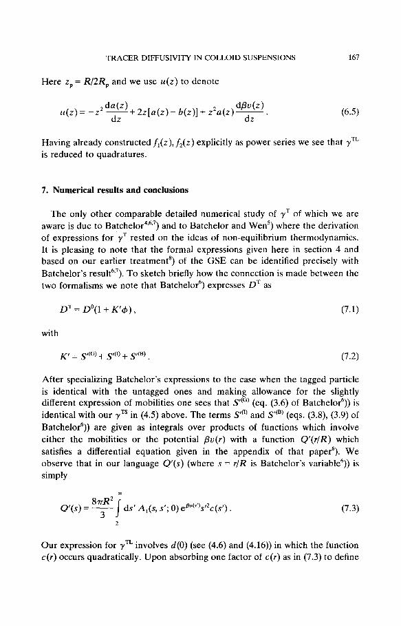
TRACER DIFFUSIVITY IN COLLOID SUSPENSIONS 161
Here zP = R/2R, and we use u(z) to denote
da(z) u(z) = -2- WV(z)
dz + 2z[a(z) - b(z)] + z2a(z) 7 .
Having already constructed fi(z), f2(z) explicitly as power series we see that yTL is reduced to quadratures.
7. Numerical results and conclusions
The only other comparable detailed numerical study of yT of which we are aware is due to Batchelor4,6*7) and to Batchelor and Wen’) where the derivation of expressions for yT rested on the ideas of non-equilibrium thermodynamics. It is pleasing to note that the formal expressions given here in section 4 and based on our earlier treatment’) of the GSE can be identified precisely with
Batchelor’s result6’7). To sketch briefly how the connection is made between the two formalisms we note that Batchelor6) expresses DT as
DT = D”(l + K’c$) , (7.1)
with
K, = c$G) + ~41) + y(B) . (7.2)
After specializing Batchelor’s expressions to the case when the tagged particle is identical with the untagged ones and making allowance for the slightly different expression of mobilities one sees that S’(‘) (eq. (3.6) of Batchelor6)) is identical with our yTs in (4.5) above. The terms S’(‘) and SrCB) (eqs. (3.8), (3.9) of
Batchelor6)) are given as integrals over products of functions which involve either the mobilities or the potential pv(r) with a function Q’(r/R) which satisfies a differential equation given in the appendix of that paper6). We observe that in our language Q’(s) (where s = r/R is Batchelor’s variable6)) is simply
m
87TR2 Q’(s) = y-- I ds’ A,(s, s’; 0) es”(s’)s’2c(s’) . (7.3)
Our expression for yTL involves d(0) (see (4.6) and (4.16)) in which the function c(r) occurs quadratically. Upon absorbing one factor of c(r) as in (7.3) to define

168 R.B. JONES AND G.S. BURFIELD
Q’ and on writing the other factor of c(r) as the sum of a part involving
mobilities and a part involving the derivative of flu(r) we obtain two con-
tributions to yTL which are respectively the same as SICB’ and S”” so that
Y n = S’PJ’ + S”“,
Batchelor and Wen’) made extensive numerical studies of a class of
potentials flu(r) more realistic than our (3.1) and using a stick boundary
condition model of the hydrodynamic interactions. They studied the regime in
which the hard core repulsion is confined to a very narrow region around the
particles corresponding to 2R < 2R, < 2.2R. In contrast we have restricted our
calculations to the regime 2.2R < 2R, in order that our mobility series give
high precision numerical results. Indeed, with stick conditions our series of
section 3 are accurate to better than one percent down to a separation r = 2.1R
but they have appreciable errors as r approaches 2R. For illustrative purposes
we present numerical results based on a choice of two different attractive
potentials corresponding to the values n = 4 and it = 6 in (3.1); in addition we
study both stick and slip hydrodynamic boundary conditions. In the results
described below we have varied the hard core radius R, in the range 2.2R <
2R, < 3.OR.
In fig. 1 we present graphs of yT, yTS, y’rL for both sets of boundary
conditions but for the case of no potential interaction outside the hard core, i.e.
N = 0 in (3.1). In fig. 2 we present similar graphs but now with an attractive
potential corresponding to n = 6 in (3.1) and with N chosen so that flu(r) = -0.5 at r = 2.2R. For such a potential there is a strong attraction between the
particles when r = 2.2R but not strong enough in relation to the thermal energy
to actually blind the pair as a doublet. As 2R, is varied out to 3R with N fixed
the strength of the potential is greatly reduced. We see that figs. 1 and 2 are
qualitatively similar with the attractive potential tail serving to reduce yT and
yTL by a few percent while increasing -yTS slightly with respect to the case of a
pure hard core without an attractive tail. The most striking feature of both sets
of curves is the contrast between stick and slip boundary conditions. In the
regime 2.2R < 2R, < 2.5R we have /yTSI > lyTLl for stick conditions while the
inequality is reversed for slip conditions. In this regime we find that /yT/ is
smaller for slip conditions than for stick conditions while for 2.8R < 2R, this
relation is reversed. For both sets of boundary conditions yT’, changes much
more rapidly than does yTS as R, is varied. To show that the details of the
potential have only a small influence we give in table V some results for the
II = 6 potential used in fig. 2 together with results for an 12 = 4 potential (again
normalized so that @(r) = -0.5 at r = 2.2R) both with stick boundary con-
ditions. These results show only small changes in yT, yTS, yn-. We cannot
directly compare our numerical results with those of Batchelor and Wen’)
because we are unable to explore reliably the region 2R, < 2.2R where most of

TRACER DIFFUSIVITY IN COLLOID SUSPENSIONS 169
-4.0
-3.0
-2.0
-1.0
2.5 3.0 2.5 3.0
2Rp'R 2Rp/R
Fig. 1. Fig. 2.
Fig. 1. Plots of yTs, yTL and yT (denoted S, L and T) for the case of a pure hard core repulsion with
R, in the range 2.2R <2Rp<3.0R. Solid lines correspond to stick and broken lines to slip
hydrodynamic boundary conditions.
Fig. 2. Plots of yTs, y” and yT (denoted S, L and T) for hard core repulsion together with a short
range attractive tail of the form flu(r) = -IV(R/~)~. The potential is normalized so that pv(2.2R) =
-0.5. As in fig. 1 solid lines denote stick and broken lines slip boundary conditions; the hard core
again lies in the range 2.2R < 2R, < 3.OR.
TABLE V Comparison of two different potentials. The constants N,, N2 are chosen so
that for both potentials @(z) = -0.50 when z = l/2.2.
flu(z) = -N,z4 flu(z) = -Nzz6
2R,lR yTs Yn YT Y TS
Y TL
Y’
2.2 -1.82 -0.40 -2.22 -1.77 -0.40 -2.17
2.3 -1.70 -0.56 -2.26 -1.65 -0.58 -2.23 2.4 -1.61 -0.74 -2.35 -1.56 -0.78 -2.34 2.5 - 1.53 -0.96 -2.49 -1.49 -1.01 -2.50 2.6 -1.46 -1.20 -2.66 -1.42 -1.27 -2.69 2.7 -1.40 -1.47 -2.87 -1.36 -1.55 -2.91 2.8 -1.34 -1.77 -3.11 -1.31 -1.86 -3.17 2.9 -1.29 -2.10 -3.39 -1.26 -2.20 -3.46 3.0 -1.24 -2.47 -3.71 -1.22 -2.58 -3.80

170 R.B. JONES AND G.S. BURFIELD
their calculations were performed. However, in the limiting case R, = R with
no attractive tail to the potential they report yT = -2.10. One can see from fig.
1 that this value is consistent with an extrapolation of our results for stick
boundary conditions.
Our two hydrodynamic models represent the extremes of strong and weak
hydrodynamic forces. Our calculations show the relative magnitude of yrs and
YTL to be strongly dependent upon the strength of these forces so that a
separate measurement of each of these components as in light scattering will
give a sensitive probe of the continuum hydrodynamic model used in suspen-
sion studies. A second conclusion is that so long as the attractive short range
tail does not bind the particles it is the hard core repulsive force which gives
the dominant contribution to yTL and moreover for 2.8R < 2R, yT’ is much
larger in magnitude than yTS. In future studies one can readily extend the series
methods of section 5 to include terms in the potential of order (R/r)’ and (R/r)’ to see the effect of longer range attractive potential interactions.
Acknowledgements
One of us (RBJ) wishes to thank Dr. Glenn Sowell for his patient and
effective instruction in the use of the MACSYMA system and Dr. Paul Kyberd
for his help in running the MACSYMA package.
Appendix
In order to see how the boundary conditions given in section 4 for the
propagator G(r, r’; s) arise we recall”) that G is the Laplace transform of a
time-dependent function G,
G(r, r’; s) = em”‘G(r, r’; t) dt . (A.11
The Green function eq. (4.14) becomes in the time domain the differential
equation
aG(r, r’; t)
at - epu(r)V- e--PL.(‘)T(r) - V($(r, r’; t) = 0 (A-2)
subject to an initial condition

TRACER DIFFUSIVITY IN COLLOID SUSPENSIONS 171
(A.3) G(r, r’; t)J,=, = 6(r - r’) .
If we introduce a function
g(r, r’; t) = e -BwG(r, #A; f) ePw)
then (A.2) and (A.3) become
ag(r, r’; t)
at - V - emBu( - V eB”“‘g(r, r’; t) = 0 .
(A.4)
(A.3
g(r, r’; t)l,,o = 6(r - r’) . (‘4.6)
However, (A.5) is the Smoluchowski equation for the relative motion of the particle pair and has the form of an equation of continuity,
ag(r, r’; t)
at + V * i(r, r’; t) = 0 , (A.7)
with a current density
j(r, r’; t) = -e-P”(‘)T(r) - VeP”“)g(r, r’; t)
= -TV Vg- T.(Vpu(r))g. (A.@
The initial condition (A.6) shows that g(r, r’; t) is simply the conditional probability that the particle pair are separated by r at time t given that they were separated by r’ at time t = 0. The current J describes the flow of this conditional probability. Thus both g and 3 must vanish within the hard core
excluded region r < 2R,. We can express j(r, r’; s) in terms of G(r, r’; s) by use of (A.1) (A.4) and (AS)
m
j(r, r’; s) = I
e-“‘i(r, r’; t) dt = -empvcr)T(r) - VG(r, r’; s) e@(“) . (A.9) 0
The vanishing of the radial probability flux r-j at the hard core separation is, in terms of G(r, r’; s), just the boundary condition (4.15). This boundary condition was incorrectly given in the appendix to our earlier paper’).
A more general model of the potential interactions than the one described here would allow finite jump discontinuities in @(r). One of us has studied’) a
model (without hydrodynamic interactions) with a continuous potential for

172 R.B. JONES AND G.S. BURFIELD
which A,(r, r’; 0) can be obtained exactly in closed analytic form and for which
as a limiting case we obtain a flu(r) with finite jump discontinuities. The
appropriate conditions on G at such a point are that the combination
G(r, r’; s) eB”(“) is continuous in both r and r’ while the flux j(, r’; s) is
continuous in r implying by (A.9) that VG(r, r’; s) has also a jump discontinuity.
References
1) P.M. Pusey and R.J.A. Tough, in: Dynamic Light Scattering and Velocimetry: Applications of
Photon Correlation Spectroscopy, R. Pecora, ed. (Plenum, New York, 1981).
2) B.U. Felderhof and R.B. Jones, Physica 119A (1983) 591. 3) W. Hess and R. Klein, Adv. Phys. 32 (1983) 173.
4) G.K. Batchelor, J. Fluid Mech. 119 (1982) 379.
5) G.K. Batchelor and C.-S. Wen, J. Fluid Mech. 124 (1982) 495.
6) G.K. Batchelor, J. Fluid Mech. 131 (1983) 155. 7) Corrigendum to refs. 4, 5 and 6, J. Fluid Mech. 137 (1983) 467.
8) R.B. Jones and G.S. Butlield, Physica 1llA (1982) 562, 577.
9) G.S. But-field, Thesis (University of London) 1984.
10) S.R. de Groot and P. Mazur, Non-equilibrium Thermodynamics (North-Holland, Amsterdam,
1962). 11) G.K. Batchelor, J. Fluid Mech. 74 (1976) 1.
12) R.B. Jones, Physica 97A (1979) 113.
13) M.M. Kops-Werkhoven and H.M. Fijnaut, J. Chem. Phys 77 (1982) 2242.
M.M. Kops-Werkhoven, C. Pathmamanoharan, A. Vrij and H.M. Fijnaut, J. Chem. Phys. 77
(1982) 5913.
14) R.B. Jones, J. Phys. A: Math. Gen. 17 (1984) 2305.
1.5) R. Zwanzig, Adv. Chem. Phys. 15 (1969) 325.
J.M. Deutch and I. Oppenheim, J. Chem. Phys. 54 (1971) 3547.
T.J. Murphy and J.L. Aguirre, J. Chem. Phys. 57 (1972) 2098.
16) J.Th.G. Overbeek, in: Colloidal Dispersions, special publication No. 43, J.W. Goodwin, ed.
(The Royal Society of Chemistry, London, 1982).
17) R. Schmitz and B.U. Felderhof, Physica 113A (1982) 90, 103.
18) R. Schmitz and B.U. Felderhof, Physica 116A (1982) 163.
19) D.J. Jeffrey and Y. Onishi, J. Fluid Mech. 139 (1984) 261.
20) J. Happel and H. Brenner, Low Reynolds Number Hydrodynamics (Noordhoff, Leiden, 1973).
21) H. Brenner, Chem. Eng. Science 16 (1961) 242.
22) E.L. Ince, Ordinary Differential Equations (Dover, New York, 1956).