Embed Size (px)
Citation preview

arX
iv:a
stro
-ph/
9811
262v
4 6
Mar
199
9
A&A manuscript no.(will be inserted by hand later)
Your thesaurus codes are:(12.03.4; 12.04.1; 12.12.1; Universe 11.03.1;
ASTRONOMYAND
ASTROPHYSICS7.2.2020
An analytic approximation of MDM power spectra in four
dimensional parameter space
B. Novosyadlyj1, R. Durrer2, V.N. Lukash3
1 Astronomical Observatory of L’viv State University, Kyryla and Mephodia str.8, 290005, L’viv, Ukraine2 Department of Theoretical Physics, University of Geneva, Ernest Ansermet, CH-1211 Geneva 4, Switzeland3 Astro Space Center of Lebedev Physical Institute of RAS, Profsoyuznaya 84/32, 117810 Moscow, Russia
Received . . . ; accepted . . .
Abstract. An accurate analytic approximation of thetransfer function for the power spectra of primordial den-sity perturbations in mixed dark matter models is pre-sented. The fitting formula in a matter-dominated Uni-verse (Ω0 = ΩM = 1) is a function of wavenumber k,redshift z and four cosmological parameters: the densityof massive neutrinos, Ων , the number of massive neutrinospecies, Nν , the baryon density, Ωb and the dimensionlessHubble constant, h. Our formula is accurate in a broadrange of parameters: k ≤ 100 h/Mpc, z ≤ 30, Ων ≤ 0.5,Nν ≤ 3, Ωb ≤ 0.3, 0.3 ≤ h ≤ 0.7. The deviation of thevariance of density fluctuations calculated with our for-mula from numerical results obtained with CMBfast is lessthan 6% for the entire range of parameters. It increaseswith Ωbh
2 and is less than ≤ 3% for Ωbh2 ≤ 0.05.
The performance of the analytic approximationof MDM power spectra proposed here is com-pared with other approximations found in the lit-erature (Holtzman 1989, Pogosyan & Starobinsky 1995,Ma 1996, Eisenstein & Hu 1997b). Our approximationturns out to be closest to numerical results in the pa-rameter space considered here.
Key words: Large Scale Structure: Mixed Dark Mattermodels, initial power spectra, analytic approximations
1. Introduction
Finding a viable model for the formation of large scalestructure (LSS) is an important problem in cosmology.Models with a minimal number of free parameters, suchas standard cold dark matter (sCDM) or standard coldplus hot, mixed dark matter (sMDM) only marginallymatch observational data. Better agreement between pre-dictions and observational data can be achieved in models
Send offprint requests to: Bohdan Novosyadlyj
with a larger numbers of parameters (CDM or MDM withbaryons, tilt of primordial power spectrum, 3D curvature,cosmological constant, see, e.g., Valdarnini et al. 1998 andrefs. therein). In view of the growing amount of obser-vational data, we seriously have to discuss the precisequantitative differences between theory and observationsfor the whole class of available models by varying allthe input parameters such as the tilt of primordial spec-trum, n, the density of cold dark matter, ΩCDM , hotdark matter, Ων , and baryons, Ωb, the vacuum energy orcosmological constant, ΩΛ, and the Hubble parameter h(h = H0/100 km/s/Mpc), to find the values which agreebest with observations of large scale structure (or even toexclude the whole family of models.).
Publicly available fast codes to calculate thetransfer function and power spectrum of fluctua-tions in the cosmic microwave background (CMB)(Seljak & Zaldarriaga 1996, CMBfast) are an essential in-gredient in this process. But even CMBfast is too bulkyand too slow for an effective search of cosmological pa-rameters by means of a χ2-minimization, like that of Mar-quardt (see Press et al. 1992 ). To solve this problem, an-alytic approximations of the transfer function are of greatvalue. Recently, such an approximation has been pro-posed by Eisenstein & Hu 1997b (this reference is denotedby EH2 in the sequel). Previously, approximations byHoltzman 1989, Pogosyan & Starobinsky 1995, Ma 1996have been used.
Holtzman’s approximation is very accurate but itis an approximation for fixed cosmological parame-ters. Therefore it can not be useful for the pur-pose mentioned above. The analytic approximationby Pogosyan & Starobinsky 1995 is valid in the 2-dimensional parameter space (Ων , h), and z (the redshift).It has the correct asymptotic behavior at small and largek, but the systematic error of the transfer function T (k) isrelatively large (10%-15%) in the important range of scales0.3 ≤ k ≤ 10 h/Mpc. This error, however introduces dis-

2 An analytic approximation for MDM spectra
crepancies of 4% to 10% in σR which represents an inte-gral over k. Ma’s analytic approximation is slightly moreaccurate in this range, but has an incorrect asymptoticbehavior at large k, hence it cannot be used for the analy-sis of the formation of small scale objects (QSO, dampedLyα systems, Lyα clouds etc.).
Another weak point of these analytic approxima-tions is their lack of dependence on the baryon den-sity. Sugiyama’s correction of the CDM transfer func-tion in the presence of baryons (Bardeen et al. 1986,Sugiyama 1995) works well only for low baryonic con-tent. Recent data on the high-redshift deuterium abun-dance (Tytler et al. 1996), on clustering at 100Mpc/h(Eisenstein et al. 1997) and new theoretical interpreta-tions of the Lyα forest (Weinberg et al. 1997) suggest thatΩb may be higher than the standard nucleosynthesis value.Therefore pure CDM and MDM models have to be mod-ified. (Instead of raising Ωb, one can also look for othersolutions, like, e.g. a cosmological constant, see below.)
For CDM this has been achieved by Eisenstein & Hu(1996, 1997a1) using an analytical approach for the de-scription of small scale cosmological perturbations in thephoton-baryon-CDM system. Their analytic approxima-tion for the matter transfer function in 2-dimensional pa-rameter space (ΩMh2, Ωb/ΩM ) reproduces acoustic oscil-lations, and is quite accurate for z < 30 (the residualsare smaller than 5%) in the range 0.025 ≤ ΩMh2 ≤ 0.25,0 ≤ Ωb/ΩM ≤ 0.5, where ΩM is the matter density pa-rameter.
In EH2 an analytic approximation of the mat-ter transfer function for MDM models is proposedfor a wide range of parameters (0.06 ≤ ΩMh2 ≤0.4, Ωb/ΩM ≤ 0.3, Ων/ΩM ≤ 0.3 and z ≤ 30).It is more accurate than previous approximations byPogosyan & Starobinsky 1995, Ma 1996 but not as pre-cise as the one for the CDM+baryon model. The baryonoscillations are mimicked by a smooth function, thereforethe approximation looses accuracy in the important range0.03 ≤ k ≤ 0.5 h/Mpc. For the parameter choice ΩM = 1,Ων = 0.2, Ωb = 0.12, h = 0.5, e.g., the systematic resid-uals are about 6% on these scales. For higher Ων and Ωb
they become even larger.
For models with cosmological constant, the motiva-tion to go to high values for Ων and Ωb is lost, and theparameter space investigated in EH2 is sufficient. Modelswithout cosmological constant, however, tend to requirerelatively high baryon or HDM content. In this paper,our goal is thus to construct a very precise analytic ap-proximation for the redshift dependent transfer functionin the 4-dimensional space of spatially flat matter domi-nated MDM models, TMDM (k; Ων , Nν ,Ωb, h; z), which isvalid for ΩM = 1 and allows for high values of Ων and Ωb.In order to keep the baryonic features, we will use the EH1transfer function for the cold particles+baryon system,
1 This reference is denoted by EH1 in this paper.
TCDM+b(k; Ωb, h), and then correct it for the presence ofHDM by a function D(k; Ων , Nν ,Ωb, h; z), making use ofthe exact asymptotic solutions. The resulting MDM trans-fer function is the product TMDM (k) = TCDM+b(k)D(k).
To compare our approximation with the numerical re-sult, we use the publicly available code ’CMBfast’ by Sel-jak & Zaldarriaga 1996.
The paper is organized as follows: In Section 2 a shortdescription of the physical parameters which affect theshape of the MDM transfer function is given. In Section3 we derive the analytic approximation for the functionD(k). The precision of our approximation for TMDM (k),the parameter range where it is applicable, and a compar-ison with the other results are discussed in Sections 4 and5. In Section 6 we present our conclusions.
2. Physical scales which determine the form ofMDM transfer function
We assume the usual cosmological paradigm: scalar pri-mordial density perturbations which are generated in theearly Universe, evolve in a multicomponent medium ofrelativistic (photons and massless neutrinos) and non-relativistic (baryons, massive neutrinos and CDM) parti-cles. Non-relativistic matter dominates the density today,ΩM = Ωb + Ων + ΩCDM . This model is usually called’mixed dark matter’ (MDM). The total energy densitymay also include a vacuum energy, so that Ω0 = ΩM +ΩΛ.However, for reasons mentioned in the introduction, herewe investigate the case of a matter-dominated flat Uni-verse with ΩM = 1 and ΩΛ = 0. Even though ΩΛ 6= 0seems to be favored by some of the present data, our mainpoint, allowing for high values of Ωb, is not important inthis case and the approximations by EH2 can be used.
Models with hot dark matter or MDM have beendescribed in the literature by Fang, Xiang & Li 1984,Shafi & Stecker 1984, Valdarnini & Bonometto 1985,Holtzman 1989, Lukash 1991, Davis, Summers & Schlegel1992, Schaefer & Shafi 1992, Van Dalen & Schaefer 1992,Pogosyan & Starobinsky 1993, 1995, Novosyadlyj 1994,Ma & Bertschinger 1994, 1995, Seljak & Zaldarriaga 1996,EH2, Valdarnini et al. 1998 and refs. therein. Below, wesimply present the physical parameters which determinethe shape of the MDM transfer function and which willbe used explicitly in the approximation which we derivehere2.
2 Recall the definitions and relationship between the MDMand the partial transfer functions
TMDM = ΩCDMTCDM + ΩνTν + ΩbTb ,
T (k) ≡δ(k, z)
δ(0, z)
δ(0, zin)
δ(k, zin),
where δ(k, z) is the density perturbations in a given componentand zin is a very high redshift at which all scales of interestare still super horizon.

An analytic approximation for MDM spectra 3
0.01 0.1 1 10
1E-8
1E-7
1E-6
1E-5
1E-4
1E-3
0.01
0.1
1
density weighted CDM baryons HDM
z=10, h=0.5, Ωb=0.18, Ων=0.4
T(k
)
k (h/Mpc)
Fig. 1. The transfer function of density perturbations of CDM,baryons and HDM at z = 10 (calculated numerically).
Since cosmological perturbations cannot grow signif-icantly in a radiation dominated universe, an importantparameter is the time of equality between the densities ofmatter and radiation
zeq =2.4× 10⁴
1−Nν/7.4h2t−4
γ − 1, (1)
where tγ ≡ Tγ/2.726K is the CMB temperature today,Nν=1, 2 or 3 is the number of species of massive neutrinoswith equal mass (the number of massless neutrino speciesis then 3 − Nν). The scale of the particle horizon at thisepoch,
keq = 4.7× 10⁻⁴√
1 + zeq h/Mpc, (2)
is imprinted in the matter transfer function: perturbationson smaller scales (k > keq) can only start growing afterzeq, while those on larger scales (k < keq) keep growingat any time. This leads to the suppression of the transferfunction at k > keq. After zeq the fluctuations in the CDMcomponent are gravitationally unstable on all scales. Thescale keq is thus the single physical parameter which de-termines the form of the CDM transfer function.
The transfer function for HDM (ν) is more compli-cated because two more physical scales enter the problem.The time and horizon scale when neutrino become non-relativistic (mν ≃ 3Tν) are given by
znr = xν(1 + zeq)− 1 ,
0.01 0.1 1 10
1E-8
1E-7
1E-6
1E-5
1E-4
1E-3
0.01
0.1
1
density weighted CDM baryons HDM
z=0, h=0.5, Ωb=0.18, Ων=0.4
T(k
)
k (h/Mpc)
Fig. 2. The same as in Fig.1 but for z=0.
knr = 3.3× 10⁻⁴√
xν(1 + xν)(1 + zeq) h/Mpc, (3)
where xν ≡ Ων/Ων eq , Ων eq ≃ Nν/(7.4 − Nν) isthe density parameter for a neutrino component becom-ing non-relativistic just at zeq. The neutrino mass canbe expressed in terms of Ων and Nν as (Peebles 1993)mν = 94Ωνh
2N−1ν t−3
γ eV.The neutrino free-streaming (or Jeans3) scale at z ≤
znr is
kF (z) ≃ 59
√
1
1 + zeq+
1
1 + zΩνN
−1ν t−4
γ h3/Mpc, (4)
which corresponds to the distance a neutrino travels inone Hubble time, with the characteristic velocity vν ≃1xν
1+z1+zeq
. Obviously, kF ≥ knr, and knr><keq for Ων
><Ων eq .
The amplitude of ν-density perturbation on smallscales (k > knr) is reduced in comparison with large scales(k < knr). For scales larger than the free-streaming scale(k < kF ) the amplitude of density perturbations grows inall components like (1 + z)−1 after zeq. Perturbations onscales below the free-streaming scale (k > kF ) are sup-pressed by free streaming which is imprinted in the trans-fer function of HDM. Thus the latter should be parame-terized by two ratios: k/knr and k/kF .
3 Formally the Jeans scale is 22.5% less than the free-streaming scale (Bond & Szalay 1983, Davis, Summers &Schlegel 1992), however, kF is the relevant physical parame-ter for collisionless neutrini.
4 An analytic approximation for MDM spectra
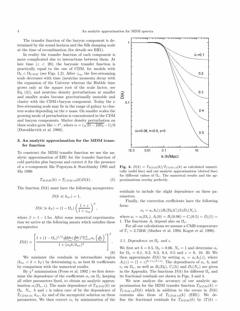
The transfer function of the baryon component is de-termined by the sound horizon and the Silk damping scaleat the time of recombination (for details see EH1).
In reality the transfer function of each component ismore complicated due to interactions between them. Atlate time (z < 20), the baryonic transfer function ispractically equal to the one of CDM, for models withΩb < ΩCDM (see Figs. 1,2). After zeq, the free-streamingscale decreases with time (neutrino momenta decay withthe expansion of the Universe whereas the Hubble timegrows only as the square root of the scale factor, seeEq. (4)), and neutrino density perturbations at smallerand smaller scales become gravitationally unstable andcluster with the CDM+baryon component. Today the νfree-streaming scale may lie in the range of galaxy to clus-ters scales depending on the ν mass. On smaller scales thegrowing mode of perturbation is concentrated in the CDMand baryon components. Matter density perturbation onthese scales grow like ∼ tα, where α = (
√25− 24Ων−1)/6
(Doroshkevich et al. 1980).
3. An analytic approximation for the MDM trans-fer function
To construct the MDM transfer function we use the an-alytic approximation of EH1 for the transfer function ofcold particles plus baryons and correct it for the presenceof a ν-component like Pogosyan & Starobinsky 1995 andMa 1996:
TMDM (k) = TCDM+b(k)D(k) . (5)
The function D(k) must have the following asymptotics:
D(k ≪ knr) = 1,
D(k ≫ kF ) = (1− Ων)
(
1 + z
1 + zeq
)β
,
where β = 1 − 1.5α. After some numerical experimenta-tion we arrive at the following ansatz which satisfies theseasymptotics
D(k) =
1 + (1− Ων)1/β 1+z
1+zeq( kF
knr)3Σ3
i=1αi
(
kkF
)i
1 + (α4k/knr)3
β
.
(6)We minimize the residuals in intermediate region
(knr < k < kF ) by determining αi as best fit coefficientsby comparison with the numerical results.
By χ2 minimization (Press et al. 1992 ) we first deter-mine the dependence of the coefficients αi on Ων keepingall other parameters fixed, to obtain an analytic approx-imation αi(Ων , z). The main dependence of TMDM (k) onΩb, Nν , h and z is taken care of by the dependence ofTCDM+b, knr, kF and of the asymptotic solution on theseparameters. We then correct αi by minimization of the
(
Ων
ΩE K ] 'N
NK0SF
Fig. 3. D(k) = TMDM(k)/TCDM+b(k) as calculated numeri-cally (solid line) and our analytic approximation (dotted line)for different values of Ων . The numerical results and the ap-proximations overlay perfectly.
residuals to include the slight dependence on these pa-rameters.
Finally, the correction coefficients have the followingform:
αi = aiAi(z)Bi(Ωb)Ci(h)Di(Nν),
where ai = ai(Ων), Ai(0) = Bi(0.06) = Ci(0.5) = Di(1) =1. The functions Ai depend also on Ων .
For all our calculations we assume a CMB temperatureof Tγ = 2.726K (Mather et al. 1994, Kogut et al. 1996).
3.1. Dependence on Ων and z.
We first set h = 0.5, Ωb = 0.06, Nν = 1 and determine αi
for Ων = 0.1, 0.2, 0.3, 0.4, 0.5 and z = 0, 10, 20. Wethen approximate D(k) by setting αi = aiAi(z), whereAi(z) = (1 + z)bi+ci(1+z). The dependences of ai, bi andci on Ων , as well as Bi(Ωb), Ci(h) and Di(Nν) are givenin the Appendix. The functions D(k) for different Ων andits fractional residuals are shown in Figs. 3 and 4.
We now analyze the accuracy of our analytic ap-proximation for the MDM transfer function TMDM (k) =TCDM+bD(k) which in addition to the errors in D(k)contains also those of TCDM+b(k) (EH1). We de-fine the fractional residuals for TMDM (k) by (T (k) −
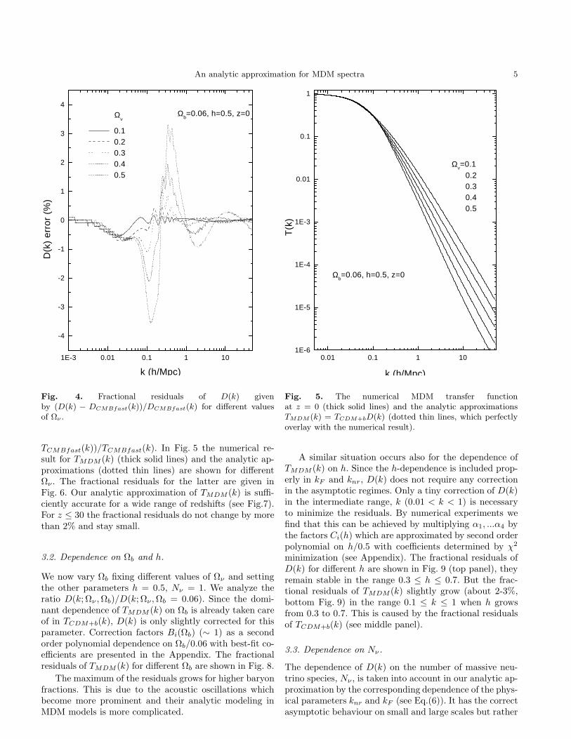
An analytic approximation for MDM spectra 5
1E-3 0.01 0.1 1 10
-4
-3
-2
-1
0
1
2
3
4
Ων
0.1 0.2 0.3 0.4 0.5
Ωb=0.06, h=0.5, z=0
D(k
) er
ror
(%)
k (h/Mpc)
Fig. 4. Fractional residuals of D(k) givenby (D(k) − DCMBfast(k))/DCMBfast(k) for different valuesof Ων .
TCMBfast(k))/TCMBfast(k). In Fig. 5 the numerical re-sult for TMDM (k) (thick solid lines) and the analytic ap-proximations (dotted thin lines) are shown for differentΩν . The fractional residuals for the latter are given inFig. 6. Our analytic approximation of TMDM (k) is suffi-ciently accurate for a wide range of redshifts (see Fig.7).For z ≤ 30 the fractional residuals do not change by morethan 2% and stay small.
3.2. Dependence on Ωb and h.
We now vary Ωb fixing different values of Ων and settingthe other parameters h = 0.5, Nν = 1. We analyze theratio D(k; Ων ,Ωb)/D(k; Ων ,Ωb = 0.06). Since the domi-nant dependence of TMDM (k) on Ωb is already taken careof in TCDM+b(k), D(k) is only slightly corrected for thisparameter. Correction factors Bi(Ωb) (∼ 1) as a secondorder polynomial dependence on Ωb/0.06 with best-fit co-efficients are presented in the Appendix. The fractionalresiduals of TMDM (k) for different Ωb are shown in Fig. 8.
The maximum of the residuals grows for higher baryonfractions. This is due to the acoustic oscillations whichbecome more prominent and their analytic modeling inMDM models is more complicated.
0.01 0.1 1 101E-6
1E-5
1E-4
1E-3
0.01
0.1
1
Ωb=0.06, h=0.5, z=0
Ων=0.1 0.2 0.3 0.4 0.5
T(k
)
k (h/Mpc)
Fig. 5. The numerical MDM transfer functionat z = 0 (thick solid lines) and the analytic approximationsTMDM (k) = TCDM+bD(k) (dotted thin lines, which perfectlyoverlay with the numerical result).
A similar situation occurs also for the dependence ofTMDM (k) on h. Since the h-dependence is included prop-erly in kF and knr, D(k) does not require any correctionin the asymptotic regimes. Only a tiny correction of D(k)in the intermediate range, k (0.01 < k < 1) is necessaryto minimize the residuals. By numerical experiments wefind that this can be achieved by multiplying α1, ...α4 bythe factors Ci(h) which are approximated by second orderpolynomial on h/0.5 with coefficients determined by χ2
minimization (see Appendix). The fractional residuals ofD(k) for different h are shown in Fig. 9 (top panel), theyremain stable in the range 0.3 ≤ h ≤ 0.7. But the frac-tional residuals of TMDM (k) slightly grow (about 2-3%,bottom Fig. 9) in the range 0.1 ≤ k ≤ 1 when h growsfrom 0.3 to 0.7. This is caused by the fractional residualsof TCDM+b(k) (see middle panel).
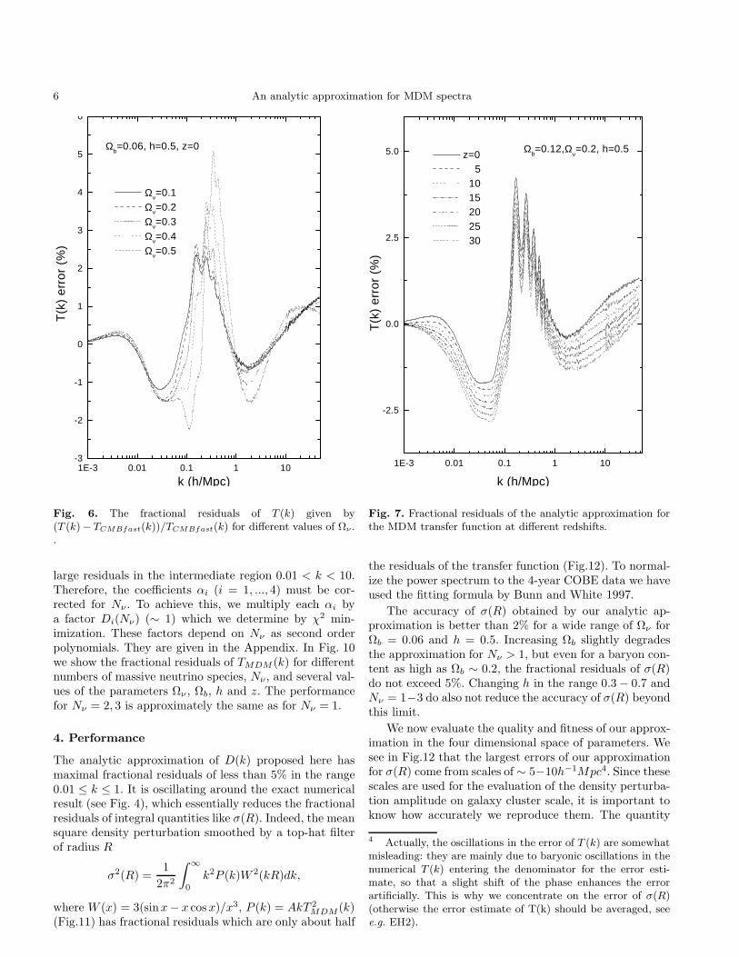
3.3. Dependence on Nν .
The dependence of D(k) on the number of massive neu-trino species, Nν , is taken into account in our analytic ap-proximation by the corresponding dependence of the phys-ical parameters knr and kF (see Eq.(6)). It has the correctasymptotic behaviour on small and large scales but rather
6 An analytic approximation for MDM spectra
1E-3 0.01 0.1 1 10-3
-2
-1
0
1
2
3
4
5
6
Ωb=0.06, h=0.5, z=0
Ων=0.1 Ων=0.2 Ων=0.3 Ων=0.4 Ων=0.5
T(k
) er
ror
(%)
k (h/Mpc)
Fig. 6. The fractional residuals of T (k) given by(T (k)− TCMBfast(k))/TCMBfast(k) for different values of Ων ..
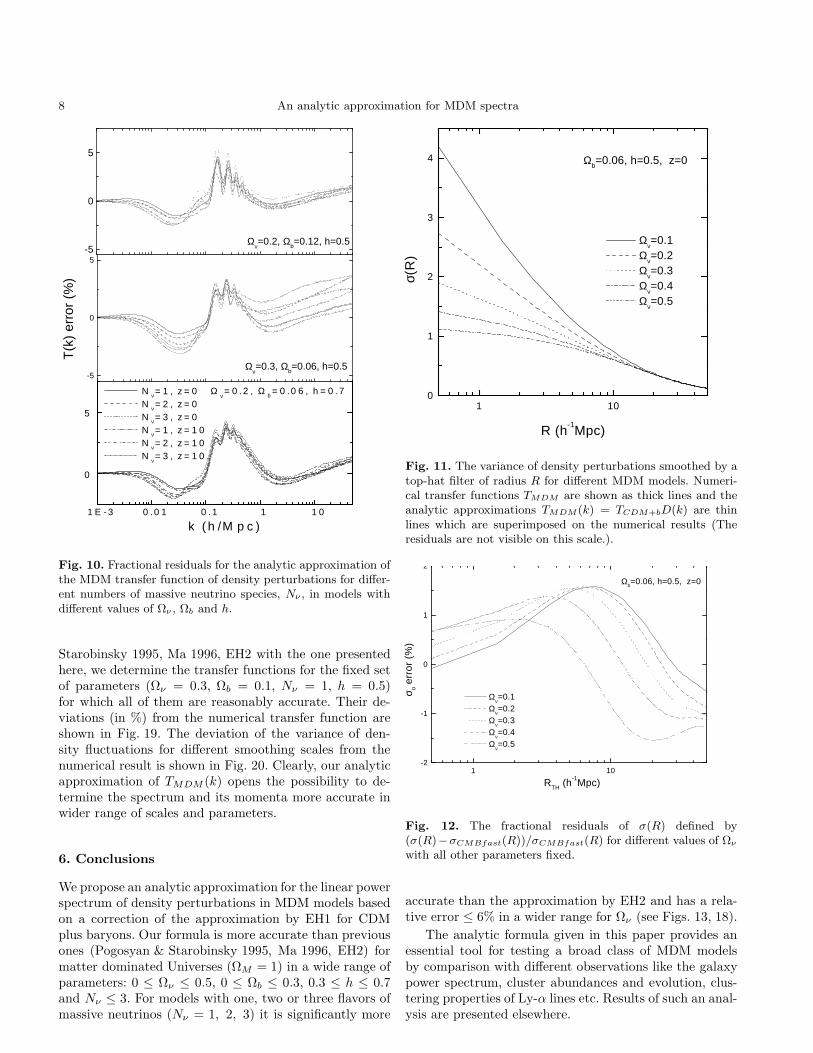
large residuals in the intermediate region 0.01 < k < 10.Therefore, the coefficients αi (i = 1, ..., 4) must be cor-rected for Nν . To achieve this, we multiply each αi bya factor Di(Nν) (∼ 1) which we determine by χ2 min-imization. These factors depend on Nν as second orderpolynomials. They are given in the Appendix. In Fig. 10we show the fractional residuals of TMDM (k) for differentnumbers of massive neutrino species, Nν , and several val-ues of the parameters Ων , Ωb, h and z. The performancefor Nν = 2, 3 is approximately the same as for Nν = 1.
4. Performance
The analytic approximation of D(k) proposed here hasmaximal fractional residuals of less than 5% in the range0.01 ≤ k ≤ 1. It is oscillating around the exact numericalresult (see Fig. 4), which essentially reduces the fractionalresiduals of integral quantities like σ(R). Indeed, the meansquare density perturbation smoothed by a top-hat filterof radius R
σ2(R) =1
2π2
∫
∞
0
k2P (k)W 2(kR)dk,
where W (x) = 3(sinx− x cosx)/x3, P (k) = AkT 2MDM (k)
(Fig.11) has fractional residuals which are only about half
1E-3 0.01 0.1 1 10
-2.5
0.0
2.5
5.0 z=0 5 10 15 20 25 30
Ωb=0.12,Ω
ν=0.2, h=0.5
T(k
) er
ror
(%)
k (h/Mpc)
Fig. 7. Fractional residuals of the analytic approximation forthe MDM transfer function at different redshifts.
the residuals of the transfer function (Fig.12). To normal-ize the power spectrum to the 4-year COBE data we haveused the fitting formula by Bunn and White 1997.
The accuracy of σ(R) obtained by our analytic ap-proximation is better than 2% for a wide range of Ων forΩb = 0.06 and h = 0.5. Increasing Ωb slightly degradesthe approximation for Nν > 1, but even for a baryon con-tent as high as Ωb ∼ 0.2, the fractional residuals of σ(R)do not exceed 5%. Changing h in the range 0.3− 0.7 andNν = 1−3 do also not reduce the accuracy of σ(R) beyondthis limit.
We now evaluate the quality and fitness of our approx-imation in the four dimensional space of parameters. Wesee in Fig.12 that the largest errors of our approximationfor σ(R) come from scales of ∼ 5−10h−1Mpc4. Since thesescales are used for the evaluation of the density perturba-tion amplitude on galaxy cluster scale, it is important toknow how accurately we reproduce them. The quantity
4 Actually, the oscillations in the error of T (k) are somewhatmisleading: they are mainly due to baryonic oscillations in thenumerical T (k) entering the denominator for the error esti-mate, so that a slight shift of the phase enhances the errorartificially. This is why we concentrate on the error of σ(R)(otherwise the error estimate of T(k) should be averaged, seee.g. EH2).

An analytic approximation for MDM spectra 7
1E-3 0.01 0.1 1 10-6
-5
-4
-3
-2
-1
0
1
2
3
4
5
6
7
8
9
10
11
Ωb
0.06 0.10 0.15 0.20 0.25 0.30
Ων=0.2, h=0.5, z=0
T(k
) er
ror
(%)
k (h/Mpc)
Fig. 8. Fractional residuals of the analytic approximation ofthe MDM transfer function for different values of Ωb.
σ8 ≡ σ(8h−1Mpc) is actually the most often used valueto test models. We calculate it for the set of parameters0.05 ≤ Ων ≤ 0.5, 0.06 ≤ Ωb ≤ 0.3, 0.3 ≤ h ≤ 0.7 andNν = 1, 2, 3 by means of our analytic approximationand numerically. The relative deviations of σ8 calculatedwith our TMDM (k) from the numerical results are shownin Fig.13-15.
As one can see from Fig. 13, for 0.3 ≤ h ≤ 0.7 andΩbh
2 ≤ 0.15 the largest error in σ8 for models with onesort of massive neutrinos Nν = 1 does not exceed 4.5% forΩν ≤ 0.5. Thus, for values of h which are followed by directmeasurements of the Hubble constant, the range of Ωbh
2
where the analytic approximation is very accurate forΩν ≤ 0.5 is six times as wide as the range given by nucle-osynthesis constraints, (Ωbh
2 ≤ 0.024, Tytler et al. 1996).This is important if one wants to determine cosmologi-cal parameters by the minimization of the difference be-tween the observed and predicted characteristics of thelarge scale structure of the Universe.
For models with more than one species of massive neu-trinos of equal mass (Nν = 2, 3), the accuracy of our an-alytic approximation is slightly worse (Fig. 14, 15). Buteven for extremely high values of parameters Ωb = 0.3,h = 0.7, Nν = 3 the error in σ8 does not exceed 6%.
-0.8
-0.4
0.0
0.4
0.8
1E-3 0.01 0.1 1 10
-1
0
1
2
3
4
TM
DM(k
) e
rro
r (%
)
k (h/Mpc)
-1
0
1
2
3
4
TC
DM
+b (
k) e
rro
r (%
)
Ων=0.2, Ωb
=0.06, z=0
h=0.3 h=0.5 h=0.7
D(k
) er
ror
(%)
Fig. 9. Fractional residuals of the analytic approximation ofD(k), TCDM+b(k) and TMDM(k) transfer function for differentvalues of the Hubble parameter, h.
In redshift space the accuracy of our analytic approx-imation is stable and quite high for redshifts of up toz = 30.
5. Comparison with other analytic approximations
We now compare the accuracy of our analytic approx-imation with those cited in the introduction. For com-parison with Fig. 12 the fractional residuals of σ(R) cal-culated with the analytic approximation of TMDM (k) byEH2 are presented in Fig. 16. Their approximation is onlyslightly less accurate (∼ 3%) at scales ≥ 10Mpc/h. InFig. 17 the fractional residuals of the EH2 approxima-tion of TMDM (k) are shown for the same cosmologicalparameters as in Fig. 16. For Ων = 0.5 (which is notshown) the deviation from the numerical result is ≥ 50%at k ≥ 1h−1Mpc, and the EH2 approximation completelybreaks down in this region of parameter space.
The analog to Fig. 13 (σ8) for the fitting formula ofEH2 is shown in Fig. 18 for different values of Ωb, Ων andh. Our analytic approximation of TMDM (k) is more ac-curate than EH2 in the range 0.3 ≤ Ων ≤ 0.5 for all Ωb
(≤ 0.3). For Ων ≤ 0.3 the accuracies of σ8 are comparable.To compare the accuracy of the analytic approxima-
tions for TMDM (k) given by Holtzman 1989, Pogosyan &
8 An analytic approximation for MDM spectra
-5
0
5
1 E - 3 0 .0 1 0 .1 1 1 0
0
5
Ων= 0 .2 , Ω
b= 0 .0 6 , h = 0 .7 N ν = 1 , z = 0
N ν = 2 , z = 0 N ν = 3 , z = 0 N ν = 1 , z = 1 0 N ν = 2 , z = 1 0 N ν = 3 , z = 1 0
k ( h /M p c )
-5
0
5
Ων=0.3, Ωb=0.06, h=0.5
T(k
) er
ror
(%)
Ων=0.2, Ω
b=0.12, h=0.5
Fig. 10. Fractional residuals for the analytic approximation ofthe MDM transfer function of density perturbations for differ-ent numbers of massive neutrino species, Nν , in models withdifferent values of Ων , Ωb and h.
Starobinsky 1995, Ma 1996, EH2 with the one presentedhere, we determine the transfer functions for the fixed setof parameters (Ων = 0.3, Ωb = 0.1, Nν = 1, h = 0.5)for which all of them are reasonably accurate. Their de-viations (in %) from the numerical transfer function areshown in Fig. 19. The deviation of the variance of den-sity fluctuations for different smoothing scales from thenumerical result is shown in Fig. 20. Clearly, our analyticapproximation of TMDM (k) opens the possibility to de-termine the spectrum and its momenta more accurate inwider range of scales and parameters.
6. Conclusions
We propose an analytic approximation for the linear powerspectrum of density perturbations in MDM models basedon a correction of the approximation by EH1 for CDMplus baryons. Our formula is more accurate than previousones (Pogosyan & Starobinsky 1995, Ma 1996, EH2) formatter dominated Universes (ΩM = 1) in a wide range ofparameters: 0 ≤ Ων ≤ 0.5, 0 ≤ Ωb ≤ 0.3, 0.3 ≤ h ≤ 0.7and Nν ≤ 3. For models with one, two or three flavors ofmassive neutrinos (Nν = 1, 2, 3) it is significantly more
1 100
1
2
3
4 Ωb=0.06, h=0.5, z=0
Ων=0.1 Ων=0.2 Ων=0.3 Ων=0.4 Ων=0.5
σ(R
)
R (h-1Mpc)
Fig. 11. The variance of density perturbations smoothed by atop-hat filter of radius R for different MDM models. Numeri-cal transfer functions TMDM are shown as thick lines and theanalytic approximations TMDM (k) = TCDM+bD(k) are thinlines which are superimposed on the numerical results (Theresiduals are not visible on this scale.).
1 10-2
-1
0
1
2
Ωb=0.06, h=0.5, z=0
Ων=0.1
Ων=0.2
Ων=0.3
Ων=0.4
Ων=0.5
σo
erro
r (%
)
RTH
(h-1Mpc)
Fig. 12. The fractional residuals of σ(R) defined by(σ(R)−σCMBfast(R))/σCMBfast(R) for different values of Ων
with all other parameters fixed.
accurate than the approximation by EH2 and has a rela-tive error ≤ 6% in a wider range for Ων (see Figs. 13, 18).
The analytic formula given in this paper provides anessential tool for testing a broad class of MDM modelsby comparison with different observations like the galaxypower spectrum, cluster abundances and evolution, clus-tering properties of Ly-α lines etc. Results of such an anal-ysis are presented elsewhere.

An analytic approximation for MDM spectra 9
-2
0
2
0.1 0.2 0.3 0.4 0.5
-2
0
2
4
Ωb=0.06 Ωb=0.10 Ωb=0.15 Ω
b=0.20
Ωb=0.25 Ωb=0.30
h=0.3, Nν=1
Ων
-2
0
2
4 h=0.7, Nν=1
σ 8 err
or
(%)
h=0.5, Nν=1
Fig. 13. Deviation of σ8 of our analytic approximation forTMDM (k) from the numerical result for different values of Ων ,Ωb and h (Nν = 1).
Our analytic approximation for TMDM (k) is avail-able in the form of a FORTRAN code and can be re-quested at [email protected] or copied fromhttp://mykonos.unige.ch/∼durrer/
Acknowledgments This work is part of a project sup-ported by the Swiss National Science Foundation (grantNSF 7IP050163). B.N. is also grateful to DAAD for finan-cial support (Ref. 325) and AIP for hospitality, where thebulk of the numerical calculations were performed. V.L.acknowledges a partial support of the Russian Foundationfor Basic Research (96-02-16689a).
-1
0
1
2
-2
0
2
4
6
h=0.7, Nν=2
σ 8 e
rro
r (%
)
0.1 0.2 0.3 0.4 0.5
-2
0
2
Ων
h=0.3, Nν=2
Ωb=0.06 Ωb=0.10 Ωb=0.15 Ω
b=0.20
Ωb=0.25 Ωb=0.30
h=0.5, Nν=2
Fig. 14. Same as Fig.13, but for Nν = 2.

10 An analytic approximation for MDM spectra
Ων
K 1ν ΩE ΩE ΩE ΩE ΩE ΩE
K 1ν
σ HU
URU
K 1ν
Fig. 15. Same as Fig.13, but for Nν = 3.
1 10-2
-1
0
1
2
3
4
Eisenstein & Hu 1997 Ωb=0.06, h=0.5, z=0
Ων=0.1 Ων=0.2 Ων=0.3 Ων=0.4
σ(R
) e
rro
r (%
)
R (h-1Mpc)
Fig. 16. Fractional residuals of σ(R) calculated by the analyticapproximation of EH2 for the same parameters as in Fig. 12.
1E-4 1E-3 0.01 0.1 1 10
-2
0
2
4
6
Eisenstein & Hu 1997Ωb=0.06, h=0.5, z=0
Ων=0.1 Ων=0.2 Ων=0.3 Ων=0.4
T(k
) e
rro
r (%
)
k (h/Mpc)
Fig. 17. Fractional residuals of the analytic approximation byEH2 of the MDM transfer function for the same parameters asin Fig.16. For comparison see Fig.6.

An analytic approximation for MDM spectra 11
0.1 0.2 0.3 0.4 0.5
-5
0
5h=0.3, N
ν=1
Ωb=0.06 Ω
b=0.10
Ωb=0.15 Ωb=0.20 Ω
b=0.25
Ωb=0.30
σ 8 e
rro
r (%
)
Ων
-5
0
5
Eisenstein & Hu 1997
h=0.5, Nν=1
σ 8 e
rro
r (%
)
-5
0
5 h=0.7, Nν=1
σ 8 e
rro
r (%
)
Fig. 18. Deviation of σ8 as obtained by the fitting formula ofEH2 from numerical results for different values of Ων , Ωb andh (Nν = 1). See Fig. 13 for comparison.
1E-4 1E-3 0.01 0.1 1 10-15
-10
-5
0
5
10 Ων=0.3, Ω
b=0.1, h=0.5
our E&H 1997b Ma 1996 P&S 1995 Holtzman, 1989
T(k
) er
ror
(%)
k (h/Mpc)
Fig. 19. Fractional residuals of different analytic approxima-tions for the MDM transfer function at z = 0 for one flavor ofmassive neutrinos.
1 10
-10
-5
0
5
Ων=0.3, Ω
b=0.1, h=0.5
our E&H 1997b Ma 1996 P&S 1995 Holtzman, 1989
σo
erro
r (%
)
RTH
(h-1Mpc)
Fig. 20. Fractional residuals of σ(R) calculated with the sameanalytic approximations as Fig. 19.
12 An analytic approximation for MDM spectra
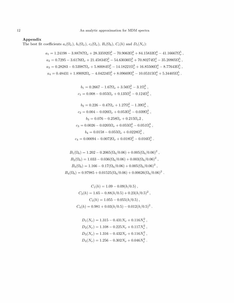
AppendixThe best fit coefficients ai(Ων), bi(Ων), ci(Ων), Bi(Ωb), Ci(h) and Di(Nν):
a1 = 1.24198− 3.88787Ων + 28.33592Ω2ν − 70.9063Ω2
ν + 84.15833Ω4ν − 41.16667Ω5
ν ,
a2 = 0.7295− 3.6176Ων + 21.45834Ω2ν − 54.63036Ω3
ν + 70.80274Ω4ν − 35.20905Ω5
ν ,
a3 = 0.28283− 0.53987Ων + 5.80084Ω2ν − 14.18221Ω3
ν + 16.85506Ω4ν − 8.77643Ω5
ν ,
a4 = 0.48431 + 1.89092Ων − 4.04224Ω2ν + 8.09669Ω3
ν − 10.05315Ω4ν + 5.34405Ω5
ν .
b1 = 0.2667− 1.67Ων + 3.56Ω2ν − 3.1Ω3
ν ,
c1 = 0.008− 0.055Ων + 0.135Ω2ν − 0.124Ω3
ν ,
b2 = 0.226− 0.47Ων + 1.27Ω2ν − 1.39Ω3
ν ,
c2 = 0.004− 0.026Ων + 0.053Ω2ν − 0.039Ω3
ν ,
b3 = 0.076− 0.258Ων + 0.215Ων2 ,
c3 = 0.0026− 0.0205Ων + 0.055Ω2ν − 0.051Ω3
ν ,
b4 = 0.0158− 0.055Ων + 0.0228Ω2ν ,
c4 = 0.00094− 0.0072Ων + 0.018Ω2ν − 0.016Ω3
ν .
B1(Ωb) = 1.202− 0.2065(Ωb/0.06) + 0.005(Ωb/0.06)2 ,
B2(Ωb) = 1.033− 0.036(Ωb/0.06) + 0.003(Ωb/0.06)2 ,
B3(Ωb) = 1.166− 0.17(Ωb/0.06) + 0.005(Ωb/0.06)2 ,
B4(Ωb) = 0.97985 + 0.01525(Ωb/0.06) + 0.00626(Ωb/0.06)2 .
C1(h) = 1.09− 0.09(h/0.5) ,
C2(h) = 1.65− 0.88(h/0.5) + 0.23(h/0.5)2 ,
C3(h) = 1.055− 0.055(h/0.5) ,
C4(h) = 0.981 + 0.03(h/0.5)− 0.012(h/0.5)2 .
D1(Nν) = 1.315− 0.431Nν + 0.116N2ν ,
D2(Nν) = 1.108− 0.225Nν + 0.117N2ν ,
D3(Nν) = 1.316− 0.432Nν + 0.116N2ν ,
D4(Nν) = 1.256− 0.302Nν + 0.046N2ν .

An analytic approximation for MDM spectra 13
References
Bardeen, J.M., Bond, J.R., Kaiser, N., and Szalay, A.S. 1986,ApJ, 304, 15
Bond, J.R., & Szalay, A.S. 1983, ApJ, 274, 443Bunn, E.F., & White, M. 1997, ApJ, 480, 6Davis, M., Summers, F.J., & Schlegel, D. 1992, Nature, 359,
393Doroshkevich, A.G., Zeldovich, Ya.B., Sunyaev, R.A. &
Khlopov M.Yu. 1980, Sov.Astron. Lett., 6, 252Eisenstein, D.J. & Hu, W. 1996, ApJ, 471, 542Eisenstein, D.J. & Hu, W. 1997a, astro-ph/9709112 (EH1)Eisenstein, D.J. & Hu, W. 1997b, astro-ph/9710252 (EH2)Eisenstein, D.J., Hu, W., Silk, J., Szalay, A.S. 1997, astro-
ph/9710303Fang, L.Z., Xiang, S.P., & Li, S.X. 1984, AA140, 77Holtzman, J.A. 1989, ApJSS, 71, 1Kogut, A., et al. 1996, ApJ, 470, 653Lukash, V.N. 1991, Annals New York Acad. of Sci., 647, 659Ma, C.-P. 1996, ApJ, 471, 13 (astro-ph/9605198)Ma, C.-P., & Bertschinger, E. 1994, ApJL, 434, L5Ma, C.-P. & Bertschinger, E. 1995, ApJ, 455, p.7Mather, J.C., et al. 1994, ApJ, 420, 439Novosyadlyj, B. 1994, Kinematics Phys. Celest. Bodies, 10, N1,
7Peebles, P.J.E. 1993, Principles of Physical Cosmology (Prince-
ton University Press)Pogosyan, D.Yu. & Starobinsky, A.A. 1993, MNRAS, 265, 507Pogosyan, D.Yu. & Starobinsky, A.A. 1995, ApJ, 447, 465Press W.H., Flannery B.P., Teukolsky S.A., Vettrling W.T.
1992, Numerical recipes in FORTRAN (New York: Cam-bridge University Press)
Shafi, Q., & Stecker, F.W. 1984, Phys.Rew.Lett., 53, 1292Schaefer, R.K., & Shafi, Q. 1992, Nature, 359, 199Seljak, U. & Zaldarriaga, M. 1996, ApJ, 469, 437 (astro-
ph/9603033)Sugiyama ApJS, 100, 281 (astro-ph/9412025).Tytler, D., Fan, X.M. & Burles, S. 1996, Nature, 381, 207Valdarnini, R., & Bonometto, S.A. 1985, AA, 146, 235Valdarnini, R., Kahniashvili T. & Novosyadlyj, B. 1998, A&A,
1998, 336, 11 (astro-ph/9804057)Van Dalen , A., & Schaefer, R.K. 1992 ,ApJ, 398, 33Weinberg, D.H., Miralda-Escude, J., Hernquist, L. & Katz, N.
1997, astro-ph/9701012
This article was processed by the author using Springer-VerlagLATEX A&A style file L-AA version 3.


![A arXiv:1511.06038v1 [cs.CL] 19 Nov 2015 · variational methods derive an analytic approximation for the intractable distribu- ... two standard test corpora. The neural answer selection](https://img.dokumen.tips/doc/110x75/600cdff0b358321ecf6c8f91/a-arxiv151106038v1-cscl-19-nov-2015-variational-methods-derive-an-analytic.jpg)