AN ANALYSIS OF THE STRUCTURE OF

TREES AND GRAPHS

A Thesissubmitted to the

University of Newcastle upon Tynefor the degree of

Doctor of Philosophy

Co R. SnowJuly 1973

The author wishes to record his thanks to all his friendsand colleagues on the staff of the Newcastle UniversityComputing Laboratory for their help and encouragement during thepreparation of this thesis. and particular~ to ProfessorsEo S. Page and Bu Randello

I am deeply indebted to Dr. ,Ho I. Scoins for his interestand helpful supervision throughout the period of researchu andfor his critical comments on the various manuscripts of thisthesiso

Thanks are also due to Hiss Eo ,Do Barraclough and theNoUoHolnGo staff for the provision of computing facilitiesu andespecially with regard to the prodoction of this thesis.

During the period of research8 I was funded from a grantfrom the Science Research Counci16 and later I was employed by

the University of Newcastle upon Tynen

This thesis is concerned with the structure of trees andlinear graphs.structure ofthem.

In particular an attempt is made to relate thethese objects to the known methods for counting

Although the work described here is essentially notcomputer oriented, the generation and decomposition of graphsand trees by computer is in the backgroundo and so a shortsection on the computer representation of the various objects isincluded.

Trees are analysed bearing in mind the counting methods duefirst to CayleY8 and a later method using Polya~s classical

theorem of enumerative combinatorial analysis., Various methodsof representation and generation of trees are presented andcompared.

This thesis then goes on to the substantially moredifficult problem of analysing graphs using similar techniques,

and attempts are made to relate the structure of graphs to theknown techniques for enumerating graphs. This involves a moredetailed study of PolyaWs theorem and an investigation into theunderlying concepts such as permutation groups as they areapplicable to the case under scrutiny. Representations aredeveloped to aid these investigations.

In the following section of the workc methods areinvestigated for the decomposition of a linear graph, and anumber of different decompositions or factorisations are looked

ato One such factorisation considered in some detail is theproblem of extracting a spanning tree from a grapho and the waysin which the remaining graph or co-tree graph may bemanipulatedo The complete decomposition of a graph into treesmay be achieved using these methodso and the concept of thestructure tree of the decomposition is introduced and itsproperties explored.

The techniques described have all been implementedp and adiscussion of the problems of the implementation together withsome estimates of timing reguirements is also includedo

Chapter 10Co~!~n!§

Introduction And Definitions 0••• o •••• o.~o.a •• a.a •• 1

Chapter II. Computer Representation ••••••• 0••• 0.00 •••• 00 •••• 15

11.1 Ordered Rooted Trees •• o ••• o •••• ncoo.oo~ ••••• n ••• n••••• 1S

II.~o1 Weight Representation o.a ••••••• oa •••••• D.o ••~.oo ••20

1102.2 Height Representation •• q.ooo9 ••o•••••• o.o.0.0D •••• 22

11.3 Relationship Between Ordered Rooted And Rooted Trees .024

11.4 Rooted And Free Trees .o•••••••••• oooo •• oa •• m ••••••• o •• 31

11.5 Linear Graphs •••••••••••••••• 0•••••••••••••••••••••• 0.32

Chapter 1110 Tree Indexing .o •• o ••• o•••• o ••••• ~oooo •• oo.no •• 037

111.1 Introduction .n •••• no.o •• ~o ••• o.a •••••••• ao.o ••••• n••• 37

111.2 Ordered Rooted Trees .oo •••••••••••••••••••• q ••••••••• 38

111.3.' Height Representation •••••• oo •• o ••• vo ••• oq.o.c.ro44

111.3.2 Weight Representation o ••• ~ ••• o ••• o.~ •••• Q.~0~.o.q52

111.4.1 Weight Representation •• Q •• ~ ••• ~ •• Q.~9 •••••••••••• 63

111.4.2 Height Representation .0 •• ~.q ••••• q ••••••• D ••••••• 72

Chapter IV. The Graph Isomorphism Problem ••••• q •• G ••••••• ~ •• 78

IV.1 The Problem D •• Q.~...D •••• 9 ••••• 0 •••• ~o•••••• ~oq •••• q •• 18

IV.2 Unger's And SussenguthWs Methods •••••••••• 0 ••••••••••• 78

IV.3 The Classification And Refinement Method ••• oq •• c ••••• r81

IV.3.1 The Refinement Algorithm ••• o •••••• qn ••••••••••••• o83

IV.4 The Automorphism Partitioning •••••••••••••••••• 0 •••••• 88

IV.4.~ The Vertex Quotient Graph ••••••••••••••••• 0 ••••••• 91

IV.4.3 The Representative And Re~ordered Graphs 0 •••••••• '00

IV.S Two Problems ••••••••••••••• o••••• o••••••• oovo •••••••• 106

Chapter Vc

V.1 Introduction oaouooa ••• o••••••• q •• !.ca ••••• a~•• 0•••• o•• 107

V.2 Relationships Between Node Labels And Line Labels ••~.q107

V.3 The Equivalence Graph •• ,•••• ~•••••• o••••• q.q •• ao ••• D •• 112

V.4 Application Of Combinatorial Techniques •• "l." •• c •• ~0".,,124

V.4.1 The Sieve Algorithm ••• o••~••qc.o.o ••••• o.~~...•..0127V.4.2 The Automorphism Group ••••••••••••••••• 0.00 •••• oq.'31

V.~ Partitions Of Graphs ••• 00 •••••••••.••• '00000 •• 0••••••• 135

Chapter VI. Factorisation o •••••••••••• oo ••0••• ~••• ~o •• ooo.o'48

VI.' General Discussion o" ••• oo~ ••oo•• o ••• oo.oooo.oo.oo.ooc148

VI Cl II <, 1 Tv 0 Al 9or i t hms o o ~ f? c Cl Cl Q Cl Cl <'. 0 c ~ () <_, 0 0 C c ~(' <: -? '? Cl c '? ~ «? Cl o Cf 0 '? 169

Chapter VII. Practical Results And Conclusions ••• o~oooa.oq~192

VII.'.1 Height Representation .ooo ••ooo.~.ooo ••• 9.o.noo.0192

VII.1.~ Weight Representation .000 •• 0.0.00 •••• 0.000 •••• 0.194

VII.2 The Canonical Ordering Algorithm ••••• o •• ooo •• a.o.~<J,:'96

VII.3 Generation Of Graphs •• n ••• ~<J.on.o•• n~ •• ~.o.~n.o •• o •• 197

VII.3.1 The Sieve Algorithm a ••• ~.an9n •• ~.~.~oa •••• ~a.nn.'98

VII.3.2 The EJuivalence Graph •••• q.9<J •••••• o •••••••••••• 198

VII.3.J The Partition Method ••o~0 •• qDqon.o •••••• o.oq.qqc20'

VII.4 Factorisation •••• 00 •••• 0 •••••••• 00 •••••••••••••••••• 202

VII.4.1 Matchings .~a ••••• oq ••••••• qo ••••• 0 ••• on.o ••••••• 203

VII.4.2 Articulation Points ••••••• 09 •• noo •••••• ooo •• o ••• 204

VII.4.J Spanning Tree Al]orithms •••• 0000 •••• 0 •• 00000 •• 00205

VII~4~4

VII. 5

VIL405 Summary

Complete

References

Conclusions

Decomposition 0C:00()OOOOOOQOOOOO<)OC>(!(,)O(JO

,207Cl c, C 0 o r- '! Cl • 00 C! 0 (.I ~ 0 C Cl 0 <? 0 0 0 0 c ~ Cl c (' 0 ~ 00 Cl Q 0 Cl e e 0 ID <;'

.206

Appendix I. .217

AI. 1

AL2

AI.3

AI,.4

AI. 5

Ordered

Rooted

Rooted

Free Trees

Graphs

Appendix II.

Counting

Rooted

Trees

Trees

Series

Trees

And GraphsFor Trees

Of Given Height

.217.~O('lO~.oOCf!~Cl~OOOOC<?OOOOOOOOC?{)0IC!O

A cc? occ>ooOqO<:.OD~qO",!oocqo

h-strongly

OClC>C'?O~~O~O()O~OOOOOCOC)OOOOOQC"I?()OOClL?t?

Regular Graphs

p.227

.229

1

The subject of Graph Theorv~~ falls naturally into threesubdivisionso We are discussing here the subject of GraphTheory in a "pure" sense, i.oe. we are disregarding theapplica tions to which Graph Theory is a useful ai d, in whichcase the subject becomes very much more diverse than just thethree subdivisions~

The first subdivision is to do simply with the ability totrove ~r not prove) theorems about graphs. This part of thesubject is very closely linked to abstract algebra and theparallels between Gra~h Theory and Discrete Mathematics mayeasily be seen c- Secondlyo Graph Theory has proved to be afruitful field for the "enumerators". There appears to be aninexhaustible supply of different types of graphr and these canall be examined with a view to counting themv and a large numberhave in fact been enumerated, FinallYr there are many problemsassociated with graphs in which it is required to find an"efficient" method of deciding whether or not a graph possesses

a certain propertYr or to find some particular property orsubgraph of a grapha

The first subdivision, then" is the province of the puremathematician and, more particularlYr of the algebraist. Thetheorems which are proved or disproved are largely of theexistence typeo or proving equivalence between properties and soon. Occasionally the proof of such an existence theoremcontains a construction of the required property or subgraphcandu even more occasionally. such a construction may be

2

gefficient' in some sense~

Secondly{ we have a large class of enumeration problemssome of which have been solved, and some of which have noteThis areao largely of interest to combinatorial analystsc hasmade some use of the al00rithmic type procedures~ but only tocompute the number of graphs of the various types. The thirdarea is studied largely by Computer Scientists. These are thepeople to whom efficiency is of prime concerne and to whom amere wave of the hand and the remark "there exists "isinsufficiento It is clear that the last class of problems canmake extensive use of much of the first arear proving theoremsto enable more efficient alqorithms to be developed,

In this thesis we embrace a little of all three. althoughwe are largely interested in the second category. We are notcontent, howeverg unlike the combinatorial analyst. simply todiscover how many there are of any particular species of graph.but also to ask: How can we produce them all? We examine herethe various combinatorial techniques which have been developedto count graphs, and try to adapt them so that they illustratebetter the way in which they correspond to the actual objectswhich they are counting, In some cases (see Page 1971) there isa method by which this can be done, particularly if there is areasonably amenable recurrence relation associated with theobjects concerned6 but when techniques such as PolyaVs theorem{Polya 19370 de Bruin 1964. Liu 1968\ are used to count theobjects it is Dot at all clear how this problem should beattacked.

3

Throughout this work, then~ we are concerned with anexamination of the structure of countable objects. and inj-a rtLcuIar with trees and linear graphs Q and attempting torelate the structural properties of these entities to theircombinatorial propertiesr wj.ththe hope that we may be able todevelop general methods for the representation and manipulationof any objects which are enumerable by current combinatorialtechnigues~

The leading work in the field of graphical enumera t.i.onhas

been done by Harary in collaboration with a number of others and

a list of some of the solved and unsolved problems in this area

are given in Harary (1Y60)t. Harary (1964)" etc, The main part

of Harary's work which is used in this thesis is his expositionof the method of counting graphs (Harary 1955). other workersin the same line are Nas~-Williams and Tutte~ A comprehensive

bibliography of the literature of enumerative graph theory isalso given by Turner(1969)o with regard to the Computer Science

interest in Graph TheorYr a paper by Read (1969) gives an

introductory survey of the types of algorithms that are beingdeveloped. The areas of interest here include Shortest PathAlgorithms (see also Pohl 1969)p Elementary Cycle Algorithms(Gotlieb and Corneil 1967p Paton 1969)0 Clique findingAlgorithms (Augustson and Minker 1970. Mulligan 1972{. Mulliganand Corneil 1972) 8 and perhaps the classic graph problem" theGraph Isomorphism problem. More recentlyv a number of uses havebeen found for graph theory to describe certain situations whicharise in computer sciencep notable in Assignment problems.Transportation problems. and also in the theory of programming.

4

program correctnessc compiler optimisation and many otherapplications~ The tree also has long been an important tool inthe syntactic analysis of programming languages and in manyother types of data representation problem (see Knuth 1968).

The present work contains a mixture of the two approachesof enumeration and aLqori,tbm production, One of the moreinteresting problems in computational graph theory is therroblem of graph isomorphism. This was the subject of a thesisby Corneil (196B) 8 in which the problem of an efficientalgorithm for isomorphism of graphs was solved for a restrictedset of graphs. Howeverc the point is made that the smallestknown graph outside this restricted set has 26 nodes. We makeuse of Corneil's algorithms in our later workr but since thesize of problem approached becomes unmanageable for graphs withconsiderably less than 26 nodesn we may employ Corneil~s

techniques in their simplest form with some confidence.

In this work we also discuss treesp particularly inchapters II and 1110 where we try to use the known combinatorial,

properties of trees to generate all of the trees of a certainsize in some convenient ordero Knuth (1968) devotes aconsiderable portion of the first volume of his book to thestudy of trees and their application to certain aspects ofcomputer scienceo such ascompilerse sorting and

data structures. parse trees forsearching and many other applications,

Other authors have studied the isomorphism problem for trees(Snow 1966 I lIIeetham'j 968) ,

with regard to combinatorial problems associated with

5

treesB the first approaches to the problem seem to have made byCayley (1889) who used an empirical method to obtain expressionsfor counting sequences for treeso CayleyVs results wereconfirmed by a different method due to Harary and Prins (1959)in which they made use of a very powerful combinatorial tool dueto Polya (1937). In chapter III we examine both methods ofcounting, but it transpires that the tree indexing problem ismuch more amenable to treatment using the Cayley method than bythe Harary and Prins method. Unfortunately. the only knownsolution to the graph counting problem is by Harary (195~) andthis makes use of Polya's theorem. which makes the graphindexing problem correspondingly more complicated" Since thepublication by Polya of his famous theoremu a large number ofcombinatorial counting problems in graph theory (and else~here)have now been solved which without the theorem seemed quiteinsoluble.

Harary (1967) gives a list of a number of unsolved problemsin graphical enumeration, which he describes as UGEP III

(revised from UGEP II (Harary 1964) and UGEP I (Barary (1960».

In chapters II and III we consider theirrepresentation and manipulationu and the ordering of trees usingthe counting methods of Cayley. In chapter IV we describe thework of Corneil on the graph isomorphism problem insofar as itis relevant to the present work. Chapter IV also contains somefurther work beyond that of corneil which we will make use of inthe following chapterv Chapter V is concerned with our attemptsto use the combinatorial methods developed by Harary and others

6

to find a method of indexing the set of non isomorphic graphs,one of which is called the Sieve algorithmo and extends theautamar phism partitioni.oq algorithm of CorneiL Chapter VIcontains a description of some methods for findingdecompositions of a qraphl and in particular. some attempts atextracting a spanning tree of a graph which is "best" in somelabelling-independent sense. The extraction of a spanning treeis in fact a special case of the factorisation of a graph. andchapter VI also contains some brief considerations of otherfactorisation problemsc The final chapter attempts to summarisethe work of the whole thesis6 together with a discussion of therractical aspects concerning some computer programs written toimplement the techniques discussed in the earlier chaptersc

We conclude this introduction by defining more formally theterms which will be used (we hope consistently) throughout this

thesis"

A g£~E!! is defined to be a set V of objec ts, known as

£Qigi~n ~QQ~ or y.~£~~~~~u toqether with a set E of ~gg~§ orli!!~2" The set E consists of pairs of elements from V, A graphis gi£~!:ed if the members of E are ordered pairs r and.I!!!Q!£~£t~gotherwise, Conventionally, a line of a directedqraph is known as an ~££. A pair (vrv) ~ Et where v ~ Vo isknown as a logE.

In an undirected graph. two nodes xc, ~ V are said to be~Qj~£~~! if there is a line (xoy) in Er and if L = (xcy) ~ Er

the line L is said to i.n.~.i.qgJ:!! with x and with ']"and x and y

are called the ~nQ=RQint§ of the line La The number of nodes to

7

which a node x is adjacent is called the Q~"<l£~~of x . A graphwhose nodes are all of the same degree is said to be ~~q~l~~.

A £~tl! in an undirected graph is a sequence of lines

o " f) "where each pair of adjacent

lines has one end-point .in common. A Q~re£i~g £!-!ih is a path ina directed graphg in which each line is directedg and thestarting node of each line is also the finishing node of thepreceding line. The length of a path is the number of lines inthe path8 and a path is said to pass through a node x if x is anend-point of at least two of the lines in the pathn A path isuni~uely defined by an ordered list of the nodes through which

it passes. A path is said to be §i!El~ if each line in the pathappears only once in the path ...and ~1~~~!!1!!£Yif each node isencountered only once. A £Y~l~ is an undirected path in whichthe starting point and the finishing point coincidee and if the

~ath is simple or elementarYn then so is the cycle (except thatthe first node coincides with the last). A directed cycle is(;enerally referred to as a ci~£~i!:0

An undirected :;raph is said to be ££!!n~£.tg~ if for every[air of nodes in the graph there is at least one path joiningthem.

In the case of directed graphsg we have several definitionsof connectedness.connected when considered as an undirected graph. A graph is~!!!1~t~I~!lY£Q~~£~~~ if for every pair of nodes ~ and~ n thereexists a (directed) path from 0(. to (!. (I or from ~ to cz. A

directed graph is said to be §!£Q!!~!Y £2!!!!g£!gg if there is a

8

~ath from any node to any other node. A graph is Qi§£Qn~~£i~Qif the condition for weak connectedness is not satisfied. For afurther discussion of directed graphs~ see Hararyo Norman and

Cartwright (1965).

A particularly important special case of an undirected~raph is a tree. A i~g!is defined as a connected graph whichpossesses no cycles. Berge (1958) shows that this definition isequivalent to a number of other properties by means of thefollowing theorem:

!h!Qr~!!L:.

Let G be a graph of order IVI = n > 1. Then any of thefollowing properties characterises a tree~

(i) G is connected and possesses no cycles.(ii) G has no cycles and has n-1 lines(iii) G is connected and has n-1 lines.(iv) G contains no cycles, and if an edge is added which

joins two non-adjacent nodes8 one (and only one) cycle isthereby formed.(v) G is connected, but loses this property if any edJe isdeleted. ,(vi) Every pair of nodes is joined by one and only one path.

We leave the reader to refer to BergeVs book (chapter 16)for the proof of this theorem. The properties given above areshown by the theorem to be equivalent8 and therefore anyone ofthem may be considered as the definition of a tree.

We define a 2y~g~~£h H of a ~raph G to be a subset U of the

9

set of nodes V. together with all those lines of G whoseend-points lie in the set u. We may define a relation P betweennodes of a graph G such that xPy holds if and only if thereexists a path in G joining the nodes x and y. In the context ofundirected graphs this relation P can easily be shown to be ane~uivalence relation. and the nodes of G are divided by PintoeSuivalence classes. where two nodes are in the same equivalenceclass if and only if the relation P holds between them. The~raph G is now partitioned into subgraphsp where each subgraphis defined by an eAuivalence class, and each of these subgraphsis conn~ted. Furthermorer there are no larger subgraphs which

are still connected. These subgraphs are known as the £Qgg~£1~~

£2~EQg~nt~ of G.

A particular case of a non-directed graph is a forest. AtQ~~2~ is any graph which has no cycles. By the definition of atreeu we see that each connected component of a forest is atree. An analogous theorem to Berge~s theorem can now be provedfor forests.

~h~Q~~~~

Let G be a graph of order IVI = n >,. Then any of thefollowing properties charactarises a forest~

(i) G has no cycles.(ii) G has p connected components and n-p lines.(iii) G i~ such tl\~t if a line is added which joinstwo non-adjacent nodesu either

(a) one and only one cycle is thereby formed,or

10

(b) the number of connected components is reduced by

one.(iv) If any line is deleted, the number of connected

components is increased by oneD(v) Every pair of nodes is joined by at most one path<

Property (i) is simply the definition of a forest.(i) ==) (ii): As already observed, the connected components of aforest are trees. Let the i-th connected component contain n~

nodes. Then we have;± n~i:i

Also, since the i-th component is a tree= n

it contains 1

lines. Thus the whole gratJht: (n,: -1) =... , - p = n - p lines •

(ii) ==) (iii): By the theorem stated earlieru no connected~raph can have less than n-1 lines and in this case it contains

no cycles (L,e D it is a tree) o If each connected componentcontains n, nodes, it must have at least n~-1 lines. But sincethe total number of lines is n-P6 each component must haveexactly nt-1 lines and therefore G contains no cycles since eachcomponent is a treeo

Now if we add one more line to G, either this line joinstwo nodes in the same component, in which case G now has exactlyone cycle. since by the previous theorem the component whichsains the line now contains exactly one cycleD and all the othercomponents are unchangedQ or else the inserted line joins two

11

nodes not in the same componentc In this caser a path nowexists which joins a node in one component to a node in anothercomponent and so these two components become a single connectedcomponent in the new graph, so that the number of components isreduced by one. This new line cannot form a cycle since if thiswere so, its two endpoints would be joined by a path notincluding the new line contradicting the assumption that the twopoints were in different components.(iii) ==> (iv): From the proof of the previous theoremp we havethe fact that if an~ line is deleted from a treeD then thenumber of components is increased from one to two. Since eachconnected component of a forest is a tree, the deletion of oneline increases the number of components in that subgraph of theforest containin0 the endpoints of the line from 1 to 2. Theremaining p-1 components are unaffected" Thus the total numberof components after deletion of the line is p+1..

fiv) ==> (v): Suppose there were two nodes having two distinct

~aths joining them. Then it would be possible to delete a linein one of the paths so that the number of components remains thesame"path.(v) ==) (i): If there was a cycle in the graph~ there would be

Thus every pair of points must be joined by at most one

two distinct paths between any pair of nodes in the cycler thusthere can be no c]cles in the :~raFho

A E~£ii~l~~£h Q of a ~raph G has the same vertex set asG, but possesses anI] a subset of the lines of GG A partialsraph G is said to §E!!Q.G., A

~jraph of a connected sraphparticularly importantG is the §£~~~ing ~~ggc

partialThis is

12

simply any partial graph of G which is also a tree. Theanalogous concept for a disconnected graph is the §£~nning~Qt~~!. A £~~!i~1~~Qg~~E~ is a partial graph of a subgraph.

trees"We will also require some general definitions relating to

A tree will sometimes be referred to as a !~~~i£~~ toemph cl. S ise the fact that it has no special properties, A £Q.9.i~Q

1£~~is a tree in which one (and only one) node has been singledout as being a reference point for the tree. This node iscalled the tQQ! of the tree. Rooted trees will be shown in thediagrams in this thesis as having their root at the bottom ofthe picture with all other nodes above the roota It now appearsto be common practice to draw trees the opposite way with theroot at the top of the diasram. There are two schools of

thought; one which says that trees should look similar tonatural trees, which have their roots in the ground~ and anotherwhich considers trees asbeing generalisations ofsuch objects as family

terminology (below" upleft" etc,) reflectsthis < ~~g.~_l_';,.

trees, In this work wesubscribe to the formerview" and our

The act of drawin~ a tree on paper immediately imposes anordering on the nodesv i.e. a"left" on the points in the diagram.

relationship of "right" andAn Q£g~g ~QQteQ i~~~

13

takes account of these spatial relationships between nodes. Infig. 1. we see two trees. both rooted. which are differentwhen considered as orderec rooted treeso but equivalent whenconsidered as rooted trees, since only the interconnection ofthe nodes and the position of the root are significant.

In a rooted tree Ii we define the J!~i.gh!.of S !!2g~ x to bethe length of the path from the node x to the root. The h~igh!.2K ~ tr~~ is the maximum height of any point in the tree , Inany tree, a node which is only adjacent to one other node in the

tree is called a !.~£mi.!!!!1node (or l~~K ), all other nodes being:r!Q!!::.l~~.I!i!!~!nodes. A tree whose root is a terminal node iscalled a E!an!~~ tree.

Two other special cases of trees are also of interest. We

define a ( ~!~i£11Y ) hin~!Y!f~~ to be a (rooted) tree in whichevery non-terminal node has exactly two nodes above ito If theroot is a terminal node then the tree consists of just this

node. Another way of expressing this is to say that either theroot has degree zeroc or the root has degree 2 and all the othernon-terminal nodes have degree 3. A property of these binarytrees is that the number of terminal nodes exceeds the number ofnon-terminals by one.

This can be shown as follows:

Let a binary tree with n nodes have t terminal nodes. Noweach node except the root has one line below Lt , Thus thenumber of lines in the tree is n--1 (which we knew anyway from

Y\o6c,

the definition of a tree>Q But each non-terminal/has two lines

14

above it. Thus the number of lines is also given by 2 (n··t).Hence

n - 1 = 2 (n .-t) art = (n + 1)/2

and the number of non-terminals is:n - (n + 1)/2 = (n - 1) /2 = t - 1c

Knuth (1968) in his book makes extensive use of a treewhich we here call a bifurcating tree. A bi!~f~ti~3 1£~~is atree in which the number of nodes above any node must not be~reater than two. This type of tree has a number ofapplications in the area of sorting and searching~

The definitions given here are those which will be referredto more commonly in later chapters. In addition6 furthercefinitions which pertain to later work are given when required.

15

It is clear that throuqhout this work on the manipulationof trees and linear graphs within a computer. some method mustbe used to identify the nodes of the graph. Thus in all ourwork whether we be dealing with labelled or unlabelled graphs wehave to attach a labelling to any graph for the purposes ofcomputer representationc The problem then becomes one of tryingto carry out manipulations in a manner which is independent ofany labelling we may impose. The other alternative is to reduceany graph to some canonical form, and then we can withconfidence use the labelling which is imposed by the canonicalform.

In some previous work (Snow 1966) we showed some ways ofrepresenting rooted trees and free trees and then using them toascertain whether two free trees were topologically equivalent<

We now describe this work with some extensions.

11.1 Ordered Rooted Trees •....---- ------ ------ ~-.-~.--~.~

The representation of ordered rooted trees requires thatsome notion of "next to" between nodes must be carried in therepresentation. We first make some definitions which areapplicable to ordered rooted trees. A E~~~~g~ is a node xtogether with all those nodes y such that x is the second node(y being the first) in the path from y to the root. The node xis said to be the Eac~~g~ hg~Q of the package. Thus 6 in fig c

100 the nodes x and n i=1uooook make up the package whose headis x. The nodes y~ are considered to be ordered within the

16

rackageo and we define the EQ§itiY~ n~i_q.h~Q~£of a node y to bethat node which is encountered next after leaving y as the nodesin the package are traversed in a clockwise sense about thepackage head~ In figo 10" the node y i..1 is the positiveneighbour of the node ~ for i=1.o~.ok-1o In this case there isno positive neighbour for Ike We define a node p to be then~g~ti~~ neighbQ~£ of the node g if and only if g is therositive neighbour of po The gE 1~f1of a node x is defined tobe that node in the package whose head is x (sometimes referredto as the package on x) which has no negative neighbour. Againreferring to fig. 1~o Y. is the negative neighbour of y~., fori=1c .006k-1 D and the node YI has no negative neighbour and is

therefore the up left of xo It is now possible to specify anordered rooted tree entirely in terms of the up left and thepositive neighbour of each of its nodes. It is also convenientto make some furtherdefinitions of relationsbetween the nodes of a

tree" In the path froma node y to the root ofthe tree" the secondnode x is called the12g!Q~of Yo Thus thebelow of y is the headof the package of whichy is a member (but notthe head) 0

x

Given the two sets of juantitieso up left and positive

17

neighbour, it is possible to deduce the values of the below foreach node, but this can involve a considerable amount of\searchin~ back~~ i~ec Operations of the type~ ufind thatelement x whose positive neighbour is the element Y'~ This typeof operation is not an easy one to perform on a computero It istherefore convenient to introduce some further information intothe quantities we have already definedo The positive neighbourvector contains information corresponding to those nodes onlywhich have a positive neighbourc and those which do noto

effectively have a blank position set aside for them" Supposenow we introduce a new vector of values called ~positive ordown'p which we will abbreviate to vpordvo This quantity can bedefined to be:

pard (x) = positive neighbour (x)= +beLo s (x)

if one existsotherwise

The minus sign is simply a marker to tell us that we are tointerpret this value as the 'below' of x rather than as the

~positive neighbour' of x" The operation of finding the below

of a node in the tree now becomes very much easier and can beillustrated in terms of the recursive function:

below ~) = if pord (x) (= 0 then - pord (x)else below (pord (x»"

We have however to be a little careful in considering thebelow of the root nodeo We may adopt anyone of a number ofconventions on thisp but in this present work it has been foundmost convenient to make the definition~

below (root) = rootand this is the only node in the tree for which this is true<

18

since the root has no positive neighbourv we also have:pord (root) = ~ root ,

It has also proved necessary to scan through the nodes of treein some sort of standard way in order to give a canonicallabelling to an unlabelled ordered rooted tree. This labellingis as follows:

1<, Label the root as node 10

2, If a node x has just been given the label io then thenode to be given the label i-t 1 is:

(a) up left of (x) if this exists(b) otherwise the positive successor of x

(pos succ (x) ) ,

When the root is reached a second time then the3, wholetree has been labelledo

The positive successor function which was used in step 2 of the

above labelling process is defined as:

= pas succ (below (x) )if it has oneotherwise

if x is the rooto20 as an exampleo we obtain the

pas succ (x) = positive neighbour of x

= x

Using the tree in figofollowing table:

Node Label 1 2 3 4 5 6 7 8 9 10 11 12

Up Left _. - 2 1 -..• 4 8 -. 12 - 6 --

PositiveNeighbour 3 - ",-" .. 5 7 9 - _-. .~ _ .. .~ 10

19

Below 4 3 4 6 6 11 6 7 11 9 11 9

Pard 3 -3 -·4 5 -, 9 -6 -7 -·11 -9 -·11 10

Pas Succ 3 5 :, 5 7 9 9 9 11 11 11 10

Position InCanonical 4 6 5 3 7 2 8 9 10 12 1 11

Ordering

This orderingr since itmakes use of the

of traversing a tree

10

positive successorrelation to such a largeextent should perhaps becalled the pp-§-i:t:iy.~

Knuth(1968) calls this method

These definitions of functions are sufficient to specify alabelled tree completelYF and further6 we are able to move bothup and down the tree without difficulty.

In the case of an unlabelled ordered rooted treep we mayrepresent this more succ.htd:ly0 This is clearly beca use we donot need to carry the relationship between node labels in ourrepresentation. Two methods of representing an unlabelled tree

20

have been devisedp both of which will be discussed in adifferent context in chapter III~

In passing it is worth notiny that the two vectors ~pord~

and 'u~l' (up left) can be regarded as the defining functionsfor a labelled tree. In fact, pord itself contains someredundant information in that the below parts of the vector can(with a certain amount of searching) be deduced from thepositive neighbour partsr However given an ~upl~ vector and aconsistent 'pardi vector we may construct functions to discoverany of the other information which we have discussed. Alsop achange in either the 'pord~ or the jupl' ve~tors would have theeffect of changing the shape of the tree. Note that sincevpord' contains some redundant informationv a change in upordv

or ~upl' may force other changes to be made to these vectors in

order to preserve consistency.

Of the two methods of representing an unlabelled treee thefirst is the weight representation ...In both of the followingrepresentations we shall use a vector of small integers todescribe the treee and in each case we assume that the i-thelement of the vector corresponds to the i~th node in thepositive ordering of the nodes of the tree.

The weight representation of a tree was introduced in ourearlier study of trees (Snow 1966) where it was described as theinteger representation. This term could equally well apply toeither of the representations to be describedu so that it was

21

thought to be a sensible idea to change the name to weightrepresentationn For any rooted tree (not necessarily ordered) c

each node in the tree is the root of some subtree (if the nodeis a terminal nodeo then the subtree consists only of that nodeand if the node is the root of the whole tree, then the subtreeis the whole tree) n Let the ~gig~1 ~~£Egsen1~1~Q~ of a tree be

the subtree whose root is the node io. It is clear that sincethe nodes are ordered according to the positive ordering of thenodes. and therefore that node 1 is the rooto we have VI = nrwhere n is the number of nodes in the complete tree. We mayalso make the observation that when labelling a tree using the

positive ordering, the root of any subtree is labelled beforeany of the other nodes in the subtree and also that once theroot of a subtree has been labelledo all the nodes in thatsubtree are labelled before any further nodes are labelledoutside that subtree. Thus, for any node j in the treec thesubtree whose root is i has a corresponding subvector in the

vector~. This subvector is of length ko where k is the numberof nodes in the subtree on j. Alsop by definitiono vJ = k.Thuse given a vector ~ which represents a treep we may chooseany element Wj I' and pick out the subvector Vj l' w~.,c< "n 0 wj~~vhere w,i

kr and this defines a subtree in the tree. Anotherinteresting property of this vector is as follows:

let P D = w'lL

p~ = W· + f: Pj for i >= 2..j:al

then ve have PI + P1 + () c. 0(1 + Pt = n' 111 where t is such that Ptdoes not refer to an element outside the vector ~n but PC+I

22

would. This is a conse1uence of the fact that if the package

whose head is the root contains the root and t other nodes" then

the n 1 nodes in the tree other than the root must all be

contained in the subtrees standing on the t other nodes in this

package n Since p~ = w~e we know that the first such subtree

contains PI nodesD and that the next tree contains p~ nodeso and

so on. This relation between members of the vector ~ also holds

within the subvectors which represent subtrees" The numbers

r~ i = 1poo.uk form a composition (or ordered partition) of the

number n -,. When we turn to the topic of the canonical

ordering of subtrees within a treeo we shall see that these

sequences of numbers p~ will become true partitions of the

number n -,. This will be dealt with in the following chaptern

The other representation to be considered here is the

height representatione Again the tree is to be represented as a

sequence or vector of small integers. We have defined the

height of a node x to be the length of the path between x and

the root of the tree. The ~e!ghi ~~E£g~gnt~tiQ~ of a tree is a

in which the nodes of the tree are

again labelled by the positive labelling. and the i-th element

of .ho h·.. is the height of the node labelled in The node 10

which of course is the rooto has height Ov and thus for any

treeo hi = O. FurtherD since we label the tree either by moving

up the tree to the next node aboveo or by moving across (and

possibly down) the tree, we have the relation h~ (= h~,+ 1 for i

23

Again we observe that since the positive labelling labelsall the nodes in a particular subtree before labelling anysubsejuent nodeso certain sUbsequences represent subtrees withinthe treem Given any node in the treeq say node jq the height ofthis node is given by h~. Now we look along thevector l! until we find another element k such that hk <= hj" andk is the smallest number greater than j for which this is true.Then the subsequence hlc~~p~.'8h~~has all its elements h~ > hin

Thus if we consider the vector hU =(h~·~h~uh.r,-hjr r ~. oh".:-hj)this is a valid height representationfor some tree. It'hisis true since the first element = h- .oh·=l& , J

Or. and if h~<= h~.I+ 10 then h~'h~ <= h~...-h.i.. 1). The vector hi

hence represents a treee and in fact it represents the subtreewhich has the node labelled j as its root. The followingtheorem demonstrates an interesting connection between theweight and height representation for trees~

For any rooted tree with n nodes8 the height vector and theweight vector are related by

consider any node kc For each node j which lies on thepath between k and the root r (including both k and r) 0 the nodek lies in the subtree of which j is the root •. Thus the node kmakes a contribution of 1 to each of the terms Wj of the vector! for each j in this path. Thus k makes a total contribution ofI Q to the sum

.....? wi c where 1.. is the number of nodes in theJ·el ..

24

path k to r. Hence the sum of all the l~ gives the total sum ofthe wi W s and thus

t: 11&It:,

= t: W·, J,j~1

the path from the node k to the rootBut the number of lines inis Ib - 1 and this is just the height of..

= L (l~ _, 1) =~:I= 0 and w, = n for

the node k , Thus...L w' 0> nj=. I

all trees with n nodesusing the fact that hiwe have

=

As has been pointed out on a number of previous occasions(Obruca 19660 Snow 19660 Scoins 1967) there is an interestingconnection between the set of ordered rooted trees of n nodes

and the set of strictly ordered rooted binary trees with nterminal nodes. It can be shown that if a binary tree has n

terminal nodes, then it has n 1 non-terminal nodes. It mayalso be shown that these two sets of trees have the samecardinality. i.e. the trees of n nodes are equinumerous with theIl,inary~rees with n terminal nodeso It is likely therefore that wecould construct a one-one mapping from one set onto the other.In fact. at least two such mappings exist. We shall describeone of themw the other being obtained by reading "right" for"left" and "left" for "right" in the following description ofthe mapping process •.

The mapping may be described recursively. Given any

25

ordered rooted tree6 we may divide it uniquely into two partsc

each of which is itself an ordered rooted tree. We arbitrarilydecide that this division is carried out by "cutting" theright-most branch at the root. Let this cut be represented by anon-terminal node of the binary tree. Fig. 3. shows the tree Tas being composed of two smaller trees TI and T~ together withthe line that will be "cut" in the decomposition process. Thetrees T. and T~ are of course ordered rooted trees in their ownriqht< In the binary tree~ we have represented the cut by anon" terminal node f' and therefore this node will have two othernodes above it, by definition of the strictly binary tree. Wenow carry out

and T a. so thatTI

the mapping process recursively on the trees T,maps onto the left subtree of the binary treec

and Ta.

riqhtmaps

subtree.onto the

If attheany stage of

recursiong the tree oneither side of the cut

is a single noden thenthis node maps onto aterminal node of thebinary tree c,

Having shown that a mapping from the set of ordered rootedt£ees of n nodes to the set of binary trees with D terminalnodes existsc and we may construct the reverse mapping withoutdifficulty, we can consider the possibility of representing anordered rooted tree in terms of a representation of itsCorr'esponding binary tree" There is a very succinct

26

representation of a binary tree, and it is thought that thismethod is approaching the minimal representation of an orderedrooted tree in terms of the information content of therepresentation and the computer storage required ..

Given a binary treell we know that each node has only twonodes above it (or none at all)c Let us represent a terminalnode by the sYllbol *u and each non-terminal node by the orderedra Lr (s,Usl..) where s. and SL are the representations of the leftand right subtrees respectively on that node .. Therepresentation of the treeo which is taken as the representationof the root noden then consists of a sequence of opening andclosing brackets and asterisks. Further_oree since there are nterminal nodes in the tree~ there are n asterisks in the

sequence. and also there are n-·'pairs of opening and closingbrackets corresponding to the non-terminals in the binary tree.

Also we know that within each pair of brackets there are exactlytwo s ub+se que nce s , which may themselves be bracketedsub-sequences or simply asterisks. Now since these bracketedsub sequences also have this propertyu we may remove the closingbrackets without any loss of informationu This is because wecan scan any such bracketed se~uence with its closing bracketsremoved frollthe left. so that each time an opening bracket isencountered we know that we must recognise two completesubsequences and then insert the corresponding closing bracket ..The following algorithm will achieve the replacement of closingbrackets.

1. Initialise by setting the input and output stringpointers to the beginning of their respective strings

27

and the stack pointer to the bottom of the stack

2. Get the next character from the input and send it to

the output strinq, It this character is an asterisk

then goto step 3. otherwise. place a zero on the top

of the stack and repeat step 2.

3, If the t.op of the stack is a zero then change it to a

one and return to step 2~ otherwise remove the top

element from the stack and send a closing bracket to

the output strin0c

4. If the stack is now empty then guitc otherwise return

to step 3,

Let us now replace each opening bracket by a 'onevr and

each asterisk by a ~zeroV< The representation of the binary

tree (and therefore of the rooted tree) is now in the form of a

sequence of zeroes and ones called a terminated binary sequence

This is a seluence of 20' 1 bits and is therefore very

economical in computer storage space.

These concepts will now be illustrated usi.nq an exanp Le ,

Consider the tree in fi~l' 2. but regard it now as an unlabelled

ordered rooted treen It is now using the positive

I'he weiqhl.

Y'III'1.

..

ordering. and the result

1·,-, '" shown in f1(1",

representation and theheight representation of

the tree are now shown

in the table below.

28

Node 1 2 3 4 5 6 7 8 9 10 11 12

Label

Weight 12 8 4 1 2 1 1 2 1 3 1 1

Re p ,

Height 0 1 2 3 3 4 2 2 3 1 2 2

Re p ,

We will now describe the steps of the mapping of theordered rooted tree into the corresponding binary tree and thento the t.~rSo. Let us denote the binary tree corresponding to atree T by 0 0 Thus if T may be decomposed intowe denote the corresponding decomposition of ~

/j'~T./ (1 then

~Y~~

As an exampleD the steps in the decomposition of the tree infig, 5(i) are given in figo 5(i)«,~ (viii),

(v) (vii)(vi)

29

(i v)

(viii)

Ei:.9.o._2~In the transition from (ii) ~o (iii)r the left subtreedecomposes into a single node on the 1efto while the rightsubtree has a single node as its right part. The growth of thebinary tree therefore stops along these branchesm The tree in

(viii) does in fact possess 12 terminals and 11 non-terminals.This tree is represented by the following sequence of bracketsand asterisks:

«*{«(*((**) C**»l*) (**») ({**)*»

which contracts to the tobo~o~110 111 0 11 00 1 000 1 00 11 00 0

Two comments may be made about this sequence. The first isthat the tob~so Contains one more ~zerot than it does 'onesvo

and in fact if ve start at the beginning of the sequence andproceed along counting the numbers of zeroes and oneso the

30

sequence terminates when the number of zeroes exceeds the numberof ones by one. Hence given any sequence of zeroes and ones. wemay pick any member of the sejuence as the starting point andextract the first subsequence which has this property" and this~epresents some ordered rooted tree, An arbitrary binaryseguence can therefore be thought of as representing a forest oftreeso provided that the sequence is terminated when a completetree has just been found.

The second observation which may be made about thet.b.s. is that correspondences may be established between thezeroes of the sequence and the nodes of the tree. and betweenthe ones of the seguence and the lines of the tree (and wenotice that there are the correct number of each). If this isdone we see that the zeroes appear in the sequence in the sameorder as their corresponding nodes appear in the positivelabelling of the tree.

It is clear that some representations will be more usefulin some contexts~ where others would be easier to use in othercontexts. The different lexicographic orderings of treesdescribed in chapter III show that a representation which givesrise to one ordering is most inconvenient when dealing with someother ordering. In facto while the tob.s. representation is bytar the most compact of those considered hereg it also appearsto be the least useful. Procedures have been written to convertfrom one representation to another for all the possiblecombinations which might be requiredo Some of these~ togetherwith a fuller discussion of the binary tree and the t.b.s. can

31

be found in Snow (1966) c

Having dealt in some detail with the representation of

ordered rooted trees6 we now describe the representation of

unordered rooted trees and free trees. In facto the only way of

t.hose described previously to represent unordered trees is the

~beloww representatione and that can only be applied to labelled

rooted treeso The techniques used to represent and manipulate

unordered rooted trees have in fact been the same as those for

ordered rooted trees6 but steps were first taken to ensure that

the ordered rooted tree was some kind of canonical form of the

unordered rooted treeo The first method used was the

representation of a rooted tree by the weight vector~ The

canonical form of this representation is obtained by sorting the

subvectors of this vector, as was described in Snow (1966) c and

which will be discussed in greater detail in chapter III. The

same sort of technique was used to reduce· a tree in height

vector representation to canonical form. Again this will be

discussed in the following chapter.

The same

representa tion

points

of free

occur

trees(!

in the discussion of

wherep in addition to

the

the

necessity for finding a canonical forme we have to impose a root

on the tree where it would not otherwise have one. Two methods

of carrying out this operation will also be explained in the

next chapter.

32

The field of representation of trees appears to beconsiderably more fruitful than the representation of linearjraphs. Howevero some of the methods of representing graphs arediscussed here brieflY6 although in the later workr theadjacency matrix was used almost exclusively as the internalrepresentation of a graph~ A more convenient method was howeverused for input of the graph~ Given a linear graph G with nnodes and m lines in which the nodes are labelled from 1 to nuand the lines are labelled from 1 to m, we may define twomatrices~

A

The first is the adjancency matrix

= (a-- where a-. = 1 if there is a"J "Jline from node i tonode j

= 0 otherwiseThe graphs dealt with here will in general be undirected. andwill not contain any line from a node to itselfo In these casesthe ad jacency IDatrix will be symmetricl, and all the elements onthe principal diagonal will be zero; . The matrix will be n " n .

The second matrix is called the incidence matrixc and is definedas

where m·· = 1\J if the node i isan endpoint of theline j

= 0 otherwise

33

Clearly this matrix is n ~ m~ Now in general a graph hasmore lines than it has points6 ioeo m>n, particularly for largeno and thus the incidence matrix occupies more space than theadjacency matrixo Neither matrix is a particularly compactrepresent.ation, since there is a considerable amount ofreduncancy in both of these representationso The adj.a.c encymatrix is (for our purposes) symmetricw and so could becompressed into the upper triangle of an n ~ n arrayu while theincidence matrix contains only two non-zero elements per column(where the columns correspond to the line labels). Obruca(1966) describes a method of storing a graph in (m + n) storagelocations. The method used for the input of a graph to ourprograms is a very small variation of Obruca's method~

Assume that the nodes are labelled from 1 to n. The graphmay be represented in terms of a vector of length (m + n 1)(for undirected graphs; (m + n) locations are required for adirected graph) 0 For each node i, the vector consists of allthe nodes j to which node i is joined, and for which j > i. Forthe nodes j such that j is joined to i and j < i, an entryappears in the section of the vector pertaining to the node joThe list for the node i is separated from the list for the nodei { 1 by some marker (such as a zero)o Thus the line from i to

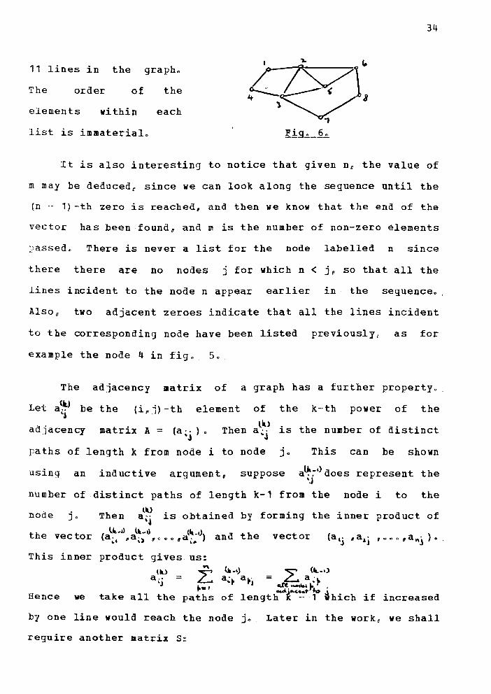
is represented by the appearance of the number j in the vectorbetween the (i·-1)-th zero and the i-th zero (assuming that i <:) c- Thus the graph in f Lq , 6. would be represented a s ;

2, 4, Ou 3, 5, 60 Ou 40 5, 7, 0, 0, 6g 00 811 0(1 au Ou

a vector of length 18"there being 8 nodes and

34

The order of thert:s?~~ a

l .,Kig.!._.§.!.

11 lines in the grapho

elements within eachlist is immaterial.

It is also interesting to notice that given no the value ofm may be deducedc since we can look along the sequence until the(n ._ 1) -th zero is reached, and then we know that the end of thevector has been found, and m is the number of non-zero elementspassedc There is never a list for the node labelled n sincethere there are no nodes j for which n < jo so that all thelines incident to the node n appear earlier in the sequence.,Alsoo two adjacent zeroes indicate that all the lines incidentto the corresponding node have been listed previously! as forexample the node 4 in fig. 5.

LetThe adjacency matrix of

a~) be the (i,j)-th elementa graph has a further property •.

the k-th power of theadjacency matrix A = (a~j). Then

oflil.)a',~J is the number of distinct

paths of length k from node i to node jo This can be shownusing an inductive argument, suppose a~;')does represent

'Jdistinct paths of length k-1 from the node i to

thenumber of the

the vectoris obtained by forming the inner product ofnode j 0

and the vectorThis inner product gives us:

(II.) ~ <. ••) "" (11..1)a. = ~ a'~ a~· = L.... a)

'') L. .. 1 ~_,L.,... ' ~.i ..., .....r~ ..take all the paths of length K - 1 which if increasedHence we

by one line would reach the node jc Later in the worko we shallrequire another matrix s:

35

5 = (s,',) where s.. is the length of the shortest path in.~the graph between nodes i and jo and this could befound by determining the smallest k such that lit.) isa v non+z e r o ,

'1Howevere even allowing for the fact that some sophisticatedmethods for multiplying matrices could be found for the simplecase when one (at least) of the matrices is purely binaryc it isclear that there are more efficient methods for deriving theelements of S available.

The whole subject of finding the shortest path between twonodes of a graph has been studied extensively (see Pohl 1969)and various algorithms have been developed (e"g~ Dijkstra

(1959) and Nicholson (1966))< For finding the elements of thematrix So howeveru Warshall-s algorithm (Warshall 1962) isrrobably the beste since we are concerned with finding theshortest distance between every pair of nodes" For the case

where we are required to find the shortest distance to everynode from so.e fixed node re some method involving the growingof a spanning tree from r is likely to be the most efficient

(see chapter VI) <>

The adjacency matrix representation of a graph proved souseful for other manipulations in the programs that no otherrepresentation was usedq except that the list representationdescribed earlier was more useful for the initial input of the~raph. A procedure was written which accepted the graph in thelist representation and output the corresponding adjacencymatrix for use by the rest of the program" Since no spaceproblems were encountered during the work (the limiting factor

36

was almost invariably computer time!) it was thought to beunnecessary to ipackv the binary adjacency matrix into less thanone matrix element per computer wordQ but clearly this couldhave been done with the conseguent reduction in efficiency dueto having to lunpacki the matrix to inspect an individual iteme

37

In this chapter an attempt is made to interpret in ameaning ful way the statement 't' I ~ "t'., where 'r. andfor each type of tree so far consideredolisting the trees of a particular type, and

't'.. are trees 6

This is done byperhaps of a

particular sLze, in some order, The objective is initially toconstruct a mapping I from the set of trees of various classesto the set of positive integers in such a way that we may definethe relation ~ as

"'!, -<",(and alsosecondly

¢:::> I (-t;) < I ('t"~)

~, = 't", C::!:> I ( 'l;') = I ("'t"",) )

to construct a straightforward algorithm to findand

this mapping I and its inverse for trees of a variety of 'sizes'and typeso Since the mapping I is intended to be an isomorphismbetween the set of trees and the set of integers between 1 and k

where k is the number of trees in the setu and since therelation < is a total ordering over the integerso the relation <is also to be a total ordering over the set of treesu ioeo forany two distinct treeseither ~, .( '"'loo

.-r. and ""...belonging to the set ..

or "'.....-< 1:',

we have

Other desirable properties of the ordering relation < over theintegers are also carried over by the isomorphismo Page (1911)describes methods of carrying out this process of constructing amapping for a wide class of objects, showingo using mainlypermutations of various types as illustrations.. how the

38

recurrence relations which are used to count these objects maybe used to generate these same objects in some orderc and alsoto give them a unique index together with an easy method ofmapping from an object to its index and back again" In the caseof trees. the counting methods are more complicated functional~xpressions, whose recurrence relations are deeply huried, andconsequently Page1s approach must be considerably extended tocope with these more complex situationso The author believesg

however, that since we have a method of counting trees ofvarious typesg and linear graphs for that matter. it should inprinciple be possihle to create an indexing scheme for all theseobjectsp by consideration of the method used to count theobjects~ We will show that using different representationso

however8 the statement ~.~ ~~ can be made meaningfulu althoughthe ordering of the trees is greatly dependent on the

representation employedc

IlL 2 Ordered Rooted Treeso._------ ------ --"'---- ------- .._--

There are several ways of indexing ordered rooted trees ofwhich the most obvious is perhaps the numerical ordering of thecorresponding tobos..when considering each toposo as a binarynumber. This method is not particularly useful since thet.b.s. is a rather specialised type of binary sequencec and thenumbers produced from the top.s.'s do not form a particularlysensible sequence of numberso However, as a first step u itdoes allow us to attach a meaning to the statement "'.0( '1:'... when ~and 'l"", are rooted trees.

39

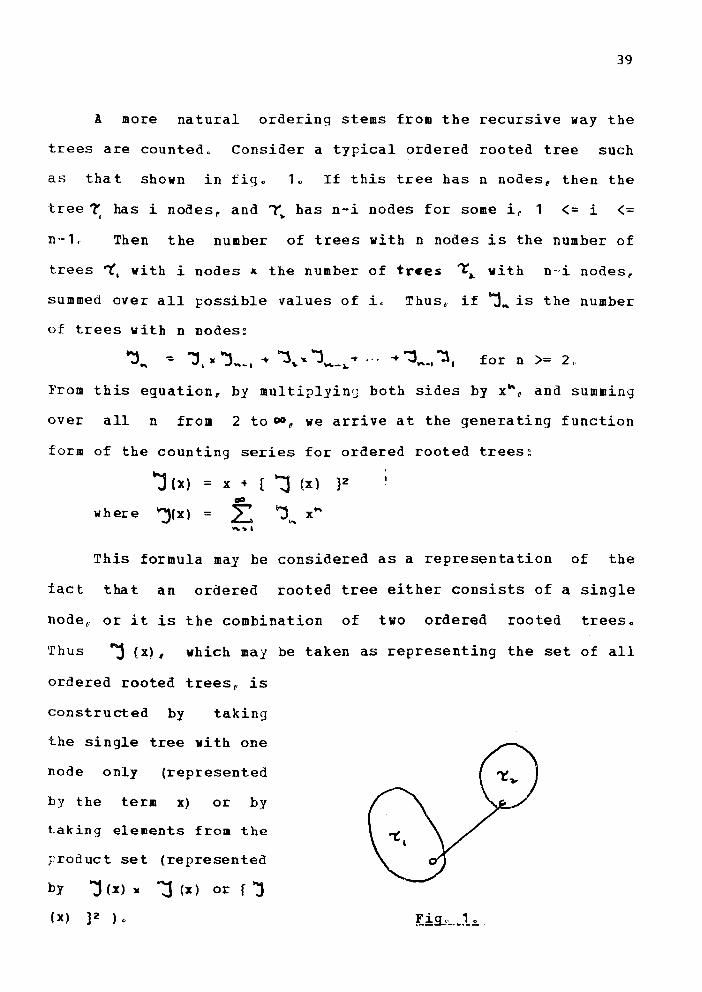
A more natural ordering stems from the recursive way the

trees are counted~ Consider a typical ordered rooted tree such

as that shown in fig. 1. If this tree has n nodes. then the

tree 7, has i nodes , and 1"'~ has n+L nodes for some it' 1 <= i <=n'-1, Then the number of trees with n nodes is the number of

trees "t, with i nodes " the number of trees 1:'J. with n-d. nodes~summed over all possible values of 10 Thusv if J...is the numberof trees with n nodes:

'j .. -: j,. J"'~I-+ j~...j~-~ .. .,. .. ':l",_, "';\I for n )= 2,

From this eguation, by multiplying both sides by Xho and summing

over all n from 2 to~o we arrive at the generating function

form of the counting series for ordered rooted trees:

j (x) = x + [ 1(x) JZ

where ~(x) = ~ ~ ....x"...... 1

This formula may be considered as a representation of the

tact that an ordered rooted tree either consists of a single

nodev or it is the combination of two ordered rooted trees.

Thus j (x), which may be taken as representing the set of all

ordered rooted treesu is

constructed by taking

the single tree with one

by the term x) or by

node only (represented

taking elements from the

product set (represented

by 1(x»)t ~ (x) or f j

(X) }2 i . !'.lli.~l~

40

Another approachp leading to the same result. is favoured

by Harary. Here we consider an ordered rooted tree to be a root

node with zero or more ordered rooted trees as its principal

su btrees , Thus, using the tera j (x) once again to represent

the set of ordered rooted treesg we have

J(X)=X (1+J(x) +{J(x) }2+{'j(x) p+.no

which gives

J(X) = x/(1 - J(x})

Now in the natural ordering of the ordered rooted trees of

n nodes, the first tree is the "join" of the tree with one node

'1. = 1) and the first tree with n -~ 1 nodes. The first tree

with n - 1 nodes may be found by the same methode i~ea it is the

"join" of the tree with 1 node and the first tree with n 2

nodes. The method then proceeds recursively until the first

tree of n nodes is found explicitly. In the general caseD to

find the k··ths. = ~j . ..., .~ j~. J ""-J

S~_I

tree of n nodeso we examine the numbers S~g where

r until we find that i such that

< k <= s·'"

We then know that the k-th tree decomposes into two parts ~I and

'T... where ~.contains i nodes and ."t'" contains n ~ i nodes. Now

there are "j, ways of choosing 'Y" and "j..._~ways of 'Y~..(jiving -:1;. J",-~ ways of constructing the tree and we

are looking for the k'-th member of this set, where

k' = k ._ s·.-.Let k be of the form (a-1) 'j . + b, where 0 < b <= j",_~ w and thus..-.we now want to look for the a-th tree in the set of trees with

i nodes and the b-th tree in the set of trees with n - i nodes~

We may now deduce these by recursive application of the above

41

methodo

Let us clarify this method by reference to an exampleoSuppose we are required to find the '70th tree in the set of

ordered rooted trees with 7 nodeso We have therefore k - 100 n= 70 From the table of the numbers ":J.. 11 we can see that

S3 = 66 t! s... = 16

and so we know that our tree consists of a subtree of 3 nodes onthe left, and one of 4 nodes on the righto In particularr sincek' = k - SI = 10 - 46 = 40 we require the 4th such tree,

Now ~3 = 2 and 1...= 51! and we may express k~ as(1 '-1) 1. + 4t' that is, the first tree with 3 nodes on the Lef t ,and the 4th tree with 4 nodes on the righto The first tree of 3nodes is the composition of the first tree with one node and thefirst tree with two nodes, Thus the left part of the requiredtree is: )according to the composition rule given in the previous chapter.

with 3 nodes composed with with thenode, this tree is therefore Vtwo gives the 70th tree with 7 nodes as:

c and the composition

Vof these

The alternative interpretation of the generating functionequation would presumably give rise to a similar method ofdetermining the k-th treet'but almost certainly to a differenttreeo In fact, since Harary1s interpretation is an infinite sumof infinite sumso it is not possible to perform this mappingfrom numbers to trees without restricting the scope of the

42

'Jenerating functions"

The first approach to the problem of indexing a set of

unordered rooted trees was made through the generation of

ordered rooted treeso By the techniques developed in our

earlier work (Snow 1966) we were able to determine whether two

ordered rooted trees were isomorphic as unordered trees,

one method of generating all rooted trees would be to generate

all ordered trees in some sequencer and reject those which were

isomorphic to trees already generated when considered as

unordered treeso This was done by reducing each tree as it was

~enerated to a canonical form as described in the aforementioned

earlier work"

This method produced a vast quantity of extra work to be

carried out by the programp since the number of ordered trees is

approximately 22~-7 for n > 4, whereas the number of unordered

trees is only about (206),,, for large no

The nu.ber of rooted trees can be calculated exactlyu and

if we let T~ be the number of trees with n nodesu and let

By the application of Polya~s theorem (Polya 1937) D a classical

theorem of enumerative combinatorial analysis which has been

explained by a number of authors (de Bruin 19640 Liu 1968c

Riordan 1958) D we know that T{x) satisfies the functionaley'uation

GO

T (x) = x exp I 2:: T (x ....) / r }'to: I

43

A more detailed discussion of Polyais theorem will be givenlaterq together with a discussion of some applications~ It wasconsidered desirable in discussing an ordering relation over aset of trees, that the structure of the trees themselves shouldbe reflected in the ordering in some way~ Thus, if we have twotrees "'(I and =., we wish to define index numbers I ('l',) and I ("l"~)

for 't, and '1'". respectively c such that I (-t:) < I ("'(J if and onlyif 't, -< "C", 1I where 't'. -< 't'"" also has an intuitively sensibleinterpreta tion withrespect to the structureof the two trees. So,by analogy with theordering of orderedrooted trees in theprevious sectionp it wasdecided to decompose thetree 1:' as shown in figo

A canonical form for~ was used which was such that if ~ is

canonical formoin canonical f ora, then 1"(. )-:'t' ..~s" G 0 'r: "t~ v and the ,( are all in

Now if two trees ~ and ~c are decomposed into

the set of trees might be~~, T~l' 0 o 08 't'L and "{Ii 6 "l" , 0" c ,'rV respectively Q then an ordering on

Jr; • ~ At'

"t:..( 1:" <.;:::::!> either "(..("C' for some j <= min (kokV)J J

and -(.:.:"(.'for i = 1,ooo(lj--1o. '"or 1:l= t1 for i = 1,,,,, '0 , k

and k < kW"

Further_oreo since this ordering is given by a recursive

44

definition, we need a starting point for the recursion, and wechoose

~ = 0 -(= '"C for all trees 1:' 0. -This ordering, which will be referred to as the naturalorderin,], does not depend in any way on the number of nodes inthe trees, so that it is meaningful to compare two trees by thismethod even if the two trees have different numbers of nodes.In the examples shown later, the number of nodes in each tree isthe sameu although the comparison as defined is equally validwhen comparing trees of different sizes.

We may define an ordering on the height representation of atree. This is simply the lexicographical ordering of the heightvectors of the trees to be comparedo In detailu this orderingis given by:

Given two trees "'(and "t' e with height vectors !! =(h,oh ... o ooo,h...) and!!' = (h.~,h!",o./Jh:)/I then 1: -< 'tv if and onlyif h < hlu where B ( hi is defined to mean

h' < h' for some 1 (= j <= nJ ,

and h~= h! for i = lcooooj-luWe demonstrate the connection between the natural ordering oftrees and the height representation ordering of a pair of treesby means of the following theoremo

The ordering imposed on the set of rooted trees by theirheight representation ordering is the same as that given by the

45

natural orderingfi

The proof is by induction on the height of the treen Thebase point for the induction in the definition of the naturalordering is the trivial tree '~o= ~ The height sequence for thistree is h = (O)e whereas any other tree has at least twoelements in its height vector, the first of which is alwayszero< This vector is therefore less than any other valid heightvector, and this is the starting point for the recursionc

Now let us consider two trees ~ and -::,ij which are

(h:u 0 c , ,h~) respectively c and let us suppose that tt decomposesinto principal subtrees 'T,,,,,. o 0 "tIL and a{w into '1:',~0 coo o~\t' Let usalso assume that 't.t-: 1:'.~ but that 1:'.= 't.u for i = 1"o<,"o)'-LJ ~ ~, • '. We

have constructed the heiqht vector in.such a way thatimplies that the corresponding vectors are equalu and thus thesequence formed by concatenating the height vectors of the

subtrees ~,oo~co~j_' is equal to that obtained by concatenatingthe height vectors of 't7 [100 ''J'ti_,o But if each element of each ofthese sequences is increased by onen and the two sequences areeach prefixed by a zeroo then the two new seguences (which arestill egual) are the partial height vectors corresponding to theroot and the subtrees "r, {! 0006 ''t'j_I respecti vely 0

Now the height sequences for ~and~ij are not equalv and by theinductive hypothesise 't'j"( 'tl if and only if hq\< h~o The partialheight vectors hand h' can now be extended by concatenating thesequences hq> and h~) in which each element has been increased by

46

one. These new partial sequences h and hi are related by

.h < h~ t=> !!(i' < h;>since we know that all the elements of h and hi which precede

start of ~) and h~iare equal.The remainder of the vectors h

and hi are irrelevant since the result of the comparison is

the

decided by the first point of difference between the vectors.Thusr by definition of the natural ordering of trees

By the inductive hypothesis

"". <. "'C.11 <=> ~,,)< h;p.. J ;a

and by the lexicographical ordering of the height sequences

In fact the theory of the height representationo and inrarticular the above theoremo applies to ordered rooted trees.We introduce it here because this representation is moreappropriate when considering the canonical form to which an

unordered rooted tree is reducedo

We must also consider the meaning of the term Qcanonicalform i with respect to the height representation. The discussionof the height vector in the previous chapter mentioned that anysubtree corresponded to some subvector of the height vector and~ave the rule for finding such a subvector. In particularu theprincipal subtrees of a tree are given by the subvectors whichbegin with the value 10 and continue until immediately beforethe next element whose value is 1n We can therefore isolate thesubvectors which represent the principal subtreeso and by the

47

above theorea, we can order the subvectors lexicographicallywithin the vector (first ensuring that each subvector is itselfin canonical form) to obtain the canonical form for the heightvector representationo which we see is the same as the canonicalform used in the natural ordering.

This natural ordering (and hence the height sequenceordering) works very well for giving a representation to theintuitive idea of ordering the trees with n nodes. but apartfrom storing an ordered list of such trees together with theirrespective index numbersl the problem of associating an indexnumber between 1 and T~r where T~ is the number of rooted treeswith n nodeso with each tree in the set still has no solutionoHoweverp we may now take a closer look at the way in which thesetrees are enumerated.

As noted earlier in section 111.2u there are at least twoways to represent an ordered rooted tree and we showed thefunctional eluations which indicated these representations. The

second of these represented the view that an ordered rooted treecan be considered as a root with zero or more ordered rootedtrees above Lt , Nowil following Harary and Prins (1959) II we maytake the same point of view with regard to rooted trees. butwith some modification. Suppose our ordered rooted tree has k

subtrees above the root" then the combinations of subtrees maybe taken from the full set of { j (x) -} , In the case of rootedtreese some of these combinations will be equivalent{ sincecertain per.utations of this set of k subtrees will not changethe tree, (The selection must also be made from the set

48

anyway) c Thus we must take into account thepermutations of the subtrees which leave the tree invariant.Polyais theorem (1937) shows how to enumerate the inequivalentmembers of this sete. without delving too deeply into the resultdiscovered by Polyar we can state that if there are k subtreesabove the roote then the number of inequivalent rooted trees is

Z (P~ ..,T (x) )

where Z is the cycle index of the symmetric group p~ ofrermutations of k objects. and where T (x) is the counting

series for rooted trees. Thus..,since a rooted tree is a rootwith zero or more subtrees above it. we have the relation

T (x) = xIt, ..

and it can be shown that-LZ(Pk6 T(x).,.0so that we have

GO

= exp { L T (XT) /s: ]..".

00

T(x) = x exp I La T{xT)/r }"'-':0

We shall discuss Polya~s theorem in greater detailn withparticular reference to the counting of linear graphs, inchapter Vo

In this method of counting trees.., we decompose the treeinto subtrees of height at most one less than the height of theoriginal t ree, This immediately suggests that there is aconnection between this counting method and the height sequencerepresentationo In fact Riordan (1960) used a very similarargument to the one of Harary and Prins given above to generatethe trees with n nodes and height he Here we denote by T l"-) (x)the generating function for rooted trees of height at most h.

49

Riordan shows that the following equation holds:_l&.) ~ t~-I)..,.T (x) = x exp { ~ T (x) Ir }

The generating function for trees of height exactly h is thengiven b y.~

By using the work of Riordan we may construct a table of valuessuch as the one given belowe in which we see the numbers oftrees with n nodes and height ho and use it to eliminate thenecessity for generating all the trees of a given size in orderto find the k-th (in the height sequence ordering) a .

n 1 2 3 4 5 6 7 8

h

1 0 1 1 1 1 1 1 1

2 1 2 4 6 10 14

3 1 3 8 18 38

4 1 4 13 36

5 1 5 19

6 1 6

7 1

We may now merely dismiss all the trees whose height is lessthan the height we are interested inc For instanceo suppose werequire the 76th tree in the height ordering of the trees with 8nodesD We see that there are 53 ( = 1 + 14 + 38) trees ofheight less than or equal to 3, and so we are now looking forthe 23rd tree (23 = 76 - 53) in the sequence of trees with 8nodes and height 4 (of which there are 36) c

Having established that the height of this tree is to be 40

we may make some remarks about the decomposition of this treeD

50

Sincer by our definition of a canonical form for a tree thefirst subtree must be the tallest. we know that this subtreemust have height = 3r Let us now consider the decompositiongiven by separating this subtree from the rest of the tree. (Wenote in passing that this is the mirror image of thedecomposition we defined earlier for ordered rooted trees) 0

Then if this first subtree "'(I has n ('r.) nodes c we deduce thatthe residue is a tree in canonical ordering with 8 ."n (--r;) nodesand height <= 4 r Lookiny at the above t.a bLe, we see that n (~)can take the values 4c Se 6 or 7 in which case the number ofj10ssibilities for '"t: is 10 3c 8 or 18 respectively" The numberof possibilities for the residue tree in these four cases is

respectively 4 (= 1 + 2 + 1)" 2 (= 1 + 1)" 1 and 1" Thiso asexpectedg gives the total number of possibilities for thisdecomposition as 1,Q -} 3,2 + 8c1 + 18,,1 = 36" Unfortunatelyc

however, the ordering of these trees which is implied by thismethod of countin] the possibilities does not correspond withthe lexicographical ordering of the height sequences" As an

exampler consider the two trees shown in figo 30 Tree (a) has ~first principal subtree which has 5 nodesv in which case it isincluded in the second term of the above expressiono whereastree ( b) has 6 nodes in its first princi.pal subtreecorresponding to the third term of the expression" We wouldlike therefore tree Ca) to precede tree (b)<. However theircorresponding height sequences are:

0 1 2 3 4 3 1 2

and0 1 2 3 4 2 3 1

51

showing that by the natural ordering v tree (b) precedes tree(a) 0

There are however methods available to generate a completelist of all the trees of n nodes in the height sequenceorderingo The most straightforward method is as follows~

,. the first tree is represented by a sequence of one zero

followed by n - 1 ones.20 from any treen we may generate the next tree in the

sequence by increasing the last element in the vector

by one8 subject to the constraint that it may notexceed its predecessor in the sequence by more than

oneo3< a check must then be made to ensure that this is a

valid rooted tree (io~o it is in canonical form). Thisis done recursively by comparing each subsequence withother subsequences at the same level in the samesub t re e ,

This algorithm was programmed and it indeed generated all therooted trees of a given sizeo but still trees were being~enerated and then rejected on the grounds that they were not incanonical form. In the case of the algorithm given abover thenumber of invalid trees generated was not nearly as high as it

52

had been when all ordered rooted trees were generated andduplicates were then rejectedr but a method was still soughtwhich would generate all the rooted trees without generatingduplicates. Scoins (1968) produced a recursive algorithm tosolve this problem, which uses the implicit stack created by therecursion to maintain back pointers to the previous subtreec

which give information about the maximum value that can be takenby each element in the hei~ht vector. This procedure thensenerates all the trees without duplicates. Although the heightvector representation appears to tie in closely with the~enerating functions which we have inspected v the relationshipwill never be entirely satisfactory while the generatingfunctions themselves contain implicit references to the numberof nodes in the tree~ By this we mean that the generatingfunction T(x) is defined to be~

T(x) - Tax" Ttx2 ..T1x3 .. "00

where the T~ are the numbers of trees with i nodes., We mighthope that the relationship with the generating function methods

of counting trees would be more closely related to a

representation in which more account is taken of the number ofnodes of each subtreec such as the weight representation to bedescribed in the next section.

Consider again the functional equation whose solution isthe generating function T(x).

T(x) = x exp { ~ T(xY')/r J.... "-1

thus

53

-log [ T(x) / x ) = 2: T(xr)/rby expanding the power series and reversing the order ofsummation, we have

DO

log [ T (x) / x ) = ~"I"~'.,"T.,.log (1 <-. X )

= 10:] I-T..,.

(1,' x") }

T (x) = x fr Cl (l o Cl 0 o (. (l r. n c:' ~.) ~,' V c. .o ~ ,( 1)

This result was however known to Cayley (1889)c who derivedit in a more empirical fashion, Cayley reasoned as follows~

Any tree of n nodes can be considered as a root, togetherwith either one tree with n - 1 nodes above it, or two trees,one with p nodes8 and one with n - 1 - p nodes above the rooto

or three trees with p, ;, and n - 1 - P ~ g nodes respectivelyabove the rooto and so OD" Thus:

T" = T"_I + >"" T., T_ + E Tt- T. TV' + <>" ~ "" 0 c ~""., o J2)~ .._, -,. "~."~".I to

Now eac h term in 2: Tt T,_ must have p >= go and furthermore v if~..t{.~"'-j

r ::;g (Leo only if n _. 1 is even) we have the term T~ ( T~ + 1)

/ 2 instead of Tr20 These restrictions are to avoid getting the

same tree twicee but on one occasion with its branches reversed"Similarly the terms L T~T, T,. must have p

p.. '\..,Y~"-'P ~ g = r we have T~{Tp + 1)/2 Tv

>= 9 >= r, and if p:= 9 ~ r or or T~ +

Alsoe if p = 1 = r8 then the appropriate term is T~ { T~+ 1 T~ + 2 } / 60 Similar restrictions must be placed onthe terms containg four or more factors. where if there are k

k.terms alikeo the term T~ must be replaced by the number ofk+coabLnations with repetition" Cayley shows that this methodof counting trees leads directly to the generating functionwhich satisfies equation (1) c

54

Examination of this generating function suggests thatpartitions are connected with this method of counting treeso andindeede each term in the equation (2) may be regarded as beingderived fro. a partition of n - 10 and thus we can consider thepossibility of ordering the trees according to an ordering ofthe partitions of n Clearlyo if the i-th part of aparticular partition is p~~ then the ordering of subtrees withina tree is tied to the ordering of the parts p~ 0

To illustrate Cayley~s method of counting treesu suppose weknow the values of Tn for n = 1oo~~o6:

we may find the value of T, by writing down all the partitionsof 6:1 1 1 1 1 1 .L T, (T, +1) (T. +2) (T, +3) (T, +4) (T. +5) = 1Co!2 1 1 1 1 T:.,l.T, (T. +1) (T, +2) (T, +3) = 1

4.2 2 1 1 t~T~ (T~ .. 1) tt T~ (T,. + 1) = 1

2 2 2 t~T:.. (T~ +1) (TL +2) = 1

3 1 1 1 T) f~T, (T. +1) (T, +2) = 2

3 2 1 T) T~ T. = 2

3 3 1. TJ (T1 .. 1) = 3J.~

4 1 1 T i.T, (T. +1) = 4.. 1.4 2 T~T\,. = 4

5 1 T,T, = 9

6 T" = 20

.,."._----48

Hence T, = 480.

55

We may now use this method of counting trees as the basisfor an ordering of all the trees of n nodesc Let us denote theset of rooted trees with n nodes by set{T~)~ The bracesunderneath the sets indicate that the trees included in anybrace correspond to a single part of the partitionoSet (TI ) = { ~ 1

T3, .,,) partitions of 1 ~-) 1

Hence set ( T'1. ) = { 1 J

Tl ._) partitions of 2 -) 1 1

) 1

1

set ( T) ) { VT~ ...> 1 1 1

2 1

3

set ( TAt ) = !'J/V Y......T~ ~.> 1 1 1 1

2 1 1

2 2

2 1 1 1

221

56

311

3 2

}

similarlyo

However it is instructive to see how the partition 3 3 of 6 is

dealt witho The contribution TJ T.l to the"sum T..,is in fact

-i T\ (T)+ 1) and not Tf c Similarly 1/ the corresponding operation in

the tree ordering gives~

if T -> IV { ) I~ T, (T, +1) -> i'(}'\y~J

i.e. we have ~ and we ensure that 't;.>~ 'l.'L. This extends

naturally to the cases where there are k equal parts in any

par t.Lt Lon ,

Using the Cayley ordering for the trees with n nodeso we

are able to associate with each number in the set { 18 00", a T ~ J a

unique treeu and this tree may be found without reference to the

other trees in the set. but only to the numbers T,VD.OoT~" We

do however require an ordering of the partitions of 2o"aDcno and

also an ordering of the combinations with repetition for many of

these numberso If all these numbers are available then we can

find the k-th tree in this orderingw whenever 1 <= k <= T~.

57

Define a tree to be of type Po where P is the partition ofthe number n ..1{'P. I P\'l' 0 o.C p.,..8 when the tree is of the formshown in fig. 4~ In the figure, the tree ~. contains p~ nodes,for i == 1,oeo,re

Now the number of trees of type P may be calculated •. Letthis number be T{P) e. Thus, Jiven an ordering for all partitionsof n - 10 and a number k, the type of the tree number k in theset of all trees of n nodes may be founde This is done bysubtracting T(P) from k for each P in orderg until the value ofk becomes negative, When this happenso we deduce that the k~thtree is of type pi whereP~ is the currentrartition in the

process. Then the k·-th

ordering. Let k~ be thelast positive value of k

in the subtraction

tree in the set of n

node trees is the k~-thtree of type P'•.

Now to find the k~-th tree of type pgu assume that pw isthe partition (PI~,P~80.~CP':'). If we take the case when all ther: are distinct, we allow the last value in this list to varymost quicklyo In other words, we take the first tree in each ofthe sets of trees with p? nodes for i = 1r.~oor-1u and take eachtree with p~ nodes in turn, and when all these trees have beencounted, we take the second tree with P~.I nodes and again take

58

all the trees with P~ nodesn If some of the p~ are equalo weare concerned with ordering the set of combinations withrepetitionnfollows:

The obvious ordering for these is simply as

Suppose we require k+conb Lnat.Lons with repetition of theelements 1pooonno Then these combinations are to be ordered bytaking the first element as 1 up to n in ordero and for eachvalue of the first element (let it be i), we take the(k-l)-combinations of the elements 10o~qoio We shall give twoexamples of the way a particular tree can be foundo

Let us first attempt to find the 27th tree with 8 nodesoBy generating the partitions of ., and counting the numbers oftrees for each partition we have:

1 1 1 1 1 1 1 1 tree

2 1 1 1 1 1 1 tree

2 2 1 1 1 1 tree

2 2 2 1 1 tree

3 1 1 1 1 2 trees

3 2 1 1 2 trees3 2 2 2 trees3 3 1 3 trees4 1 1 1 4 trees4 2 1 4 trees4 3 8 trees

As these partitions are generatede the corresponding number oftrees are subtracted from the value 27, and before the lastpartition (4 3) is generated, the value has been reduced to 6e

59

and thus would go negative on subtraction of the number (8) oftrees with this partition. Hence. we now are looking for the6th tree with partition 4 30 Already part of the weight vectorfor the resulting tree can be set up:

w = (8u4u' .'-0"031/-0'»

dashes represent values whichLet the trees with 4 nodes be

where the have yet to bethedetermined. denoted by

numbers 1,2t3c4o and the trees with 3 nodes be denoted by theletters a,b. then the combinations which we can have are (inorder) 'la, 'lh , 2ac Zb, 3aD 3b. 4a, 4bo Now the 6th tree in thissequence is the tree denoted by 3b. i.e..the 3rd tree in the setof trees with 4 nodeso and the second tree with 3 nodes. In thesame way as beforer we may find the find the 3rd tree with 4nodes by enumerating the partitions of 3~

.1 1 1 1 tree2 1 1 tree3 2 trees

The third tree in this sequence is then the first tree with

partition 30 which itself corresponds to the first partition of2~ i~eQ 1 1.. Our weight vector now becomes:

.~ = (8 t: 4 "3 ~1 D 1 I' 3 I - 0 -. )

To fill in the last two dashes in this vector" we nowinspect the second tree with 3 nodesv i.e. ,the tree b above.This corresponds to the second tree partition of 2 (since thefirst partition of 2 represents only one tree), and this in turnmakes reference to the first partition of 10 Thuso the weightvector has the final form~

~ = (Bu403r1c''t3,;2.,1).

60

The other example to be considered is to find a tree from alarger set of trees" Let us consider the determination of the121st tree in the set of tree with 12 nodes" By the samecounting process of partitions as before, it is found that the121st tree with 12 nodes is the 16th tree with partition 4 4 3.The set of trees with this partition consists of 20 trees" andwe again denote the trees of 4 nodes by 102.3 and 40 and thetrees of 3 nodes by a and b. The 2-combinations of 1v2,3.4v inorder6 are:

1 1, 2 1 0 2 2p 3 1{' 3 28 3 36 4 1" 4 2/' 4 30 4 4,.

But each of these combinations has to be used in conjunction\liththe two trees a and ba The final result of picking out the16th tree in this set gives that the required tree is made up ofthe trees 4 2 b, Le. the fourth tree with 4 nodes, the secondtree with four nodes and the second tree with 3 nodes. This

gives rise to the weight vector~

! = (12040362010402010103.,201) 0

The two trees generated by this method in the two examples given

are shown in fig. 5.

The weight vector referred to here is of course the

61

weight representation which has already been described inchapter lIe Although the weight representation is the mostnatural to use when discussing CayleyVs ordering of trees6 thisordering unfortunately does not quite correspond exactly withthe lexicographical ordering of the weight vectorso This isbecause we have considered Cayley~s ordering as fixing apartition at level 1 of the tree and allowing the partitions atlevel 2 to vary through all their possible values. However. bythe strict lexicographical ordering of the weight vectors apartition at level 2 may have to be fixed while the later partsof the first level partition may have to be changed. Weillustrate this with an example. Consider the two trees shown

in fig. 6.

F~g~_Q~

Tree (a) clearly comes before tree (b) in the ordering by weightvectors v since their respective weight representations are~

(a) 7 4 1 1 1 2 1

and~

(b) 7 4 2 1 1 1 1but the first level partition for tree (a) is 4 2 while that fortree (b) is 4 1'. The weight representation ordering can ofcourse be modified by making the comparison of elements of the

62

weight vectors in a slightly different order" For instanceu ifwe compare the weight.vectors of the two trees in fig" 6,.,in aterm by

(Q.l (10)term fashiono we find that w~ < 'Ill and hence we deducethat tree (a) comes before (b) in the orderingo If however we

(...., lit). (pjfirst compare 'II I If 'II. and then wa 6

~)these pairs equal we then compare V~ .... ~ =

w~and on finding both of~<'0.) \"'~ l'-lw1....= w,-with Wc. we find

that tree (b) is now less than tree (a)" The full algorithm forscanning the weight vector in this order is~

1, compare the first element of each vector, and if these

are differentu the result of the comparison between thetwo trees is the result of this comparison; otherwi.se"

2 " Set i = 2 o and k = W I 0

Compare and wl.'~)and if these differ then the result~

is the result of this comparison; otherwiseu

Set i :: i lo.)+ w. c..

If i <= k then return to step 3;(Ao)

Set i = smallest value such that w. has not yet been,considered and set ("')k = w~_. ; if there is such an iv

return to step 3; otherwise the algorithm terminateswith the result that the two trees are equalo

Using this algorithmD the trees to be compared are examined inthe same way as they are generated in the Cayley orderingo bylooking at the whole partition at one level before movingfurther up in the tree structureo The same result could beachieved by defining the weight vector in such a way that thenodes are labelled in a different ordero vizn by labelling allthe nodes at one level of the tree before labelling tbe nodes atany higher level., If the weight vector were defined in this

63

wayo the lexicographic ordering of the weight vectors wouldcorrespond exactly with the Cayley ordering of the treeso Theuse of the word level is quite consistent since the nodescorresponding to values within a single partition all have thesame height valueo

In the two previous sections, we have been able to orderthe corresponding types of tree according to some representationboth of the trees themselves, and of the numbers "l", and T..o Thereason why this was possible was that we were able to expressthe numbers 1", and To.in terms of a sum of products of earliernumbers in the same sequence" That iSQ we have been able toshow that trees of n nodes could be described in terms of treewith n -,1 or less nodes. In the following dLsc ussdon, we haveto modify our method slightll since we have to take account ofsubtraction operations which appear in the counting formulae forfree trees"

The most easily described formula for the generatingfunction for free trees is due to otter (1948) and is alsoreferred to by Riordan· (1958)0, If

wheret(x) = tax + t&X2 + tix3 + t~x· + OQ~

is the number of free trees with i nodese then it canbe shown that t(x) satisfies the equation

t(x) = T{x)." -if T2(x) ~ T(x2) }

6~

Riordan, in his description of the derivation of this eguationp

defines the £~~!£oiQ of a treeo and this is the same as the£~~i£~of n~!Q~£as defined by Cayley (1889) 0

Given a free tree, at any point in the tree we have anumber of lines incident to ito Each such line determines asubtree of the treeD and the number of nodes in each of thesesubtrees is known as the weight of that subtreeo Let theweights of the subtrees at some node x be av be c. etc. where a)= b >= c >= n ~ • Then at b + c + = n - ·1 where the treecontains n nodes n Now if a > ~ n, the subtree which correspondsto the weight a (let us call it B (a}) is said to be P'£~do.~.!!!~l!£.If a = In (which implies that n is even) c then B(a) is said to

~be !~£~!! .g.QJ!i!!~.l!1Dand if a < t n then all the subtrees B (a)r

B (b){I B (c)8 roo are said to be §!!J2ggy~!.

Given any tree with n nodes, if n is odd then there is oneand only one node for which the subtrees are subegualn If n isevenr then either there is one and only one node for which thesubtrees are sube~ualD or else there is no such point. but thereare two adjacent points both of which have a merely dominantsubtreeo and all the other nodes have a predominant subtree .

.~£22.t;,. (cayley)

Clearlyo if n is odd there can be no merely dominantsubtree, since this implies that a = in for some nodeo but amust be an integer. Thus it remains to show that there is one

65

and only one node with all its subtrees subequal~

Starting at any node, the values a , be ClOP" may becaLc uLated for that node, If a < ~ n c then we have a centre of

number (at least one)" otherwisee move to the adjacent point

in the subtree B(a). For this node we may now calculate the(,uantities a i I b i 8 c~ r V" 0 and one of these quantities is equalto 1 + b + c + Thus a~ <= a - 10 So we can move about thetree, each time moving into the predominant subtreeu until wereach a point for which the subtrees are subequalo We now haveto show that there is only one such node" Suppose there are twosuch nodes x. and x~0 Then x. has subtrees B (a,)0 B (b,)r B (Cl) 0

and x2 has subtrees B(aa,)uB(b1)c B(cl,)u <.~" Now a, < tnoand therefore bl + c, + UOo > j. n-L

1Now the node Xl must be in

one of these subtreesu and hence a~ cannot be less than 1 + bl +

CI

+ > !ne contradicting the assumption that all the1.

subtrees at xl.are aubequa'l, Thuse for n odd e there exists aunique point whose subtrees are subequal

For the case where n is even, the argument proceeds exactlyas before6 except that there may be a situation when a = ~nn forsome node 0 Carry out the process as described above, until aFaint is found whose subtrees are subegual. r e , howevero a nodeis found such that a = in (and b + c + c 0 0 = in 1) we now

). 1-

proceed to the adjacent point in the subtree B (a)0 Now we findaij b 1/ 6 C I I Cl ~ ~ where a~ = 1 + b + c + " 0 0 = tno L~" we have0

found a pair of adjacent nodes both having merely dominantsubtrees. The proof that these are the only such pointsproceeds as before.

66

Cayley defines the point with all its subtrees subequal tobe the £~~~~~ Q1 nQ~bg£D or in the case where there are twoadjacent nodes with merely dominant subtrees these two nodestogether with the line joining them are defined as the Q;i::£~!l~!:~of ~~!£~~ These two nodes are sometimes referred to separately

usesthe terms ceA!!!:Q.igand .11i:.:£~n..t£Q.!g for the centre and bi·~centreof number respectively"

In attempting to generate all free treesu we may generateall rooted trees and reject all those for which the root doesnot coincide with the centroid, or with one of the half~centresof numbero In this latter case8 we are faced with the problemof deciding which of the two ways in which a free tree may berepresented as a rooted tree we should rejecto Howevero by thetheoremu we know that there can be no such trouble as long as

the tree has an odd number of nodeso

Returning to Otter~s formula for the number of free trees~

we can expand the formula to obtain an explicit expression forthe number t"D the number of free trees with n nodes"

t.. = Tn - I L T~~ - T",~} / 2fo+C\. ~ ...

(T..b.= 0 if n isodd)

or= T - 2: T T if n is odd.. ">'j," '\= T..- ~ TL. ~ -- .1. T2, + J. T~ r -,. ~ "B \... .. ,).

">i\.= T 1:T~T,_ t T..tJT..,,,,-1) if n is even,

,,>C\..of counting trees is based on the definition of theThis methodcentroid (or centre of number}o Suppose now that each tree isto be considered as two partso the left-most subtree above the

67

rooto and the remainder of the tree, as shown in figo 7v

Assume that the tree is in canonical form for rooted trees asdefined by the Cayley ordering< Then if the number of nodes in

the left-most subtree is

centroid" (This follows

Fr and p < n/2l' then theroot of the tree is the

from the definition ofcentroid)" Now considerthe case when n is odd.Then if p is the number of nodes in the left subtreer theremainder of the tree contains 9 (= n - p) nodeso Now for theroot of this tree to be the centroid we must have p < n/2 and q) n/2u ioe< p + q = nand p < qv Hence if p > q this tree isexcluded from the list of free trees e and so the term - ET~~,.~appears in the counting expression for t~. In the case where nis even a further term comes in to the reckoning. In this caseit is possible for p to be equal to n/2" For this value of Po

the tree has no centroid8 but it has a bi-centroid. and acorrection term is required in the expression for tn to ensurethat the same free tree does not get counted twice -,when theroot is at each end of the bi-centroid. As we saw whenexamining the counting methods for rooted treesp if two parts ofthe tree were of equal weight I' the correspondLnq term in thecounting expression was tT~,~(T"J~+ 1 and not T2

'

0..... So in thiscaseo all the trees which decompose into subtrees such that p =q := n/2 are a set of T!,..trees c of which only ~ ~JT~,...+ 1) are..required. i~e. from the set of all T~ rooted trees with n nodes

68

we must omit (in addition to those for which p > n/2)1) of the trees where p = n/20 This then accounts for theappearance of this term in the expression for t~ when n is even.

This study of the countin~ expressions for the t~ leadsdirectly on to a method of generating the free trees with nnodes in ordera If n is odd6 we generate all the free treesfrom the set of rooted trees without having to reject any. inthe case where n is even. some of the generated trees will haveto be rejectedc but this is only for the trees which have abi-centroid. and there is reason to believe that the set oftrees with bi-centroids is relatively small. and less than halfof these have to be discarded. In n is odd then. we know fromCayleyVs theorem that each tree has a centroido Hence the freetrees may be represented by those partitions of n-1 for whichthe largest part Po < \. ne Thus/Jif only these partitions are'1enerated. we generate only the free trees. In the case where nis even, we may again generate the partitions for which P. <

n/2o but we must now go on to look at the partitions which giver, = n/20 and be must be somewhat more careful when looking atthe trees to which they correspondo These are the trees withbi.vcent roLds, and here they must all be generated and anyduplicates must be rejectedo Cayley also gives the numbers oftrees with bi-centroids and centroids and from this set ofnumbers we see that the set of trees possessing a bi··centroid isrelati vely small. (These numbers will be given later in theAppendix) 0 A second reason why it is relatively inexpensive todiscard some of the trees with bi-centroids is that the methodof deciding whether to throw a tree away is trivial •.

69

If a tree has been generated for which p, = n/21J we knowthat

ItL P' = n/2 1,:~

since this tree is represented by a partition of n -. 10 Now thesecond level partition in the first subtree may be compared veryeasily with the remainder of the whole tree~. Again wearbitrarily decide that if we have a tree with a bi-centroid wereject this tree if the first subtree is less (in the sense ofour ordering) than the remainder of the tree~

Two examples will again help to clarify the points made

By looking at the seguence of trees of 7 nodes in theCayley or d e r Ln q , we are interested in the trees whose weightvector !! has the value 3 or less for w~ Q and we see that thereare 11 of themo exactly the same number as the number of freetrees of 7 nodes" Explicitly these trees are:

7 1 1 1 1 1 1

7 2 1 , , 1 1

7 2 1 2 1 1 1

7 2 1 2 1 2 1

7 3 1 1 1 1 1

7 3 2 1 1 1 1

7 3 1 1 2 1 1

7 3 2 1 2 1 1

7 3 1 1 3 1 1

7 3 2 1 3 1 1

7 3 2 1 3 2 1

70

These trees are drawn out in fig~ 80

We can also see the relationship between the other trees in theset of rooted trees with 7 nodes, and the terms in theexpression for t~v

t..,= T."._Tt.T,~ T(Tl~ T...Tl= 48 ~ 20 )( 1 - 9 " 1 - 4 )( 2 = 11

and we can see in the full set of rooted trees the trees whosefirst level has Pi ~ 60 5 and 4 respectively~

The other example illustrates what happens in the case whenthe trees have bi-·centroids~. Here we take the trees with 8nodeso The trees for which the first level partition haslargest part p equal to 3 are generated as in the previousexampleu but we need to look more closely at those trees withthe value 4 as the second element of the weight vectors,

The total number of such trees is 16 :: (4) 2 = T~l7and theyare:

8 4 1 1 1 1 1 1 *8 4 2 1 1 1 1 1 &

8 4 3 1 1 1 1 1 &

8 4 3 2 1 1 1 1 &

8 4 1 1 1 2 1 1

71

8 4 2 1 1 2 1 1 *8 4 3 1 1 2 1 1 &

8 4 3 2 2 1 1 &

8 4 1 1 3 1 1

8 4 1 1 1 3 2 1

8 4 2 1 1 3 1 1

8 4 2 1 1 3 2 1

8 4 3 1 1 3 1 1 *8 4 3 1 1 3 2 1

8 q 3 2 1 3 1 1 &

8 4 3 2 1 3 2 1 *Of these, those which are marked with an asterisk have the twoparts to be compared egual to each other u and thus they must beincluded in the set of free trees. Those that are marked withan ampersand are those whose first subtree aDd remainder parts

"t', and -t~ respectively are related by 't,)o" 't~~ These also haveto be included in the set of free trees. It will be seen thateach tree in the set of those marked with an ampersand has a

dual in the set of those unmarked •. Figo. 9Q shows these trees.

~w ~

'\Y'J Xl0

Fi_g.!:..~~

72

There is another special point in a free tree which can beidentifiedo This point is the centre of the treeo From eachnode in the treeo there is one and only one path to every otherpoint in the tree (by the definition of a tree) D Let thedistance between any two nodes be the length of the path joiningthose two nodeso The ~i~~~t~£of a tree is defined to be thesreatest distance between any two nodes in the treeD If thediameter is eveno then there is a node at the mid~point of thediameter, and this point is called the £~1~~ of the treeo Ifthe diameter of the tree is odde then there is a middle line inthe path, and this line together with its two end'-points is

called the hi=£~!!~o

The centre or hi-centre of a tree is uniguea

Suppose there are two centrese i.ea there are two distinctpaths each equal in length to the diameter which have distinctmid-points x, and x). Let y, and y~ each be an extremity of thepath with mid-points x, and x~ respectivelyo such that thediameters do not intersect between x, and y, or between x~ andy~u and let the length of each diameter be 2rD Then thedistance from x, to y, e and from x~ to y, is r in each caseoBut since the tree is connected and x, and x~ are distinct,there must be a path of length d (> 0) from x, to x~o and hence

73

the path from y, to y~ must pass through XI and x~ and itslength is equal to r + d + r > 2r~ contradicting the statementthat the original 'diameters' were of maximum length.

The proof for the uniqueness of the hi-centre is almostidentical~

One algorithm for finding the centres or hi-centre of atree is to remove all the terminal nodes and the lines to whichthey are joined to give a reduced tree~ This VstrippingV

process may now be repeated on the reduced treen and so onn

until either one or two nodes remaino In these cases we havefound the centre or b~-centre of the tree respectively. It isclear that this algorithm will terminate with the correct resultsince each iteration removes one line from each end of everydiameter, and that the definition of diameter implies that thisprocess will take at least as many iterations to remove all thelines from a diameter as are required to remove all the lines

from any other path in the tree., Since a line is removed fromeach end of a diametern the algorithm terminates when the middleof the dia.eter is reached.

It is possible to determine whether the root of a rootedtree coincides with its centreo or with one end of thebi"centrec This operation again becomes trivial if the tree isheld in its height representation. Ifn howeverr free trees arebeing generated by finding such trees in the set of rootedtreese some care must again be taken to ensure that duplicatesare not accepted due to the root being at one end of the

74

bi~centre. In the canonical form of a tree according to theheight representation~ the principal subtrees planted at theroot are ordered by their height. Thus the first two subtreesare the highesto If in any rooted tree the height of the firsttwo subtrees are e~ual, then the root of this tree is at itscentre. If the height of the first two subtrees differ by one(i.e. the first subtree has height one greater than the secondsubtree) then the root is at one end of the bi-centre of thetree. Let us assume that the tree has the form shown in fig.10. In this case the root is at one end of the bi~centreo andwe know that the height of the first subtree is one greater thantbe height of the second subt.r'ee, L~o h('tJ = h('t'4.)owhere h('t')is the maxillullheiqht of the tree"¥n Now if "(e>- = "t'feo then thesame free tree rooted at the other end of its bi~centre would beidentical as a rooted tree 0 However 0 if "t'...1 '!'.o then rootingthe tree at the opposite end of its bi-centre would give twoaistinct rooted trees. Thusw precautions must be taken toensure that when a tree

is found whose root iscoincident with one endof the bi·-centreo a

previous tree is notbeing duplicatedu Thiscan be prevented by

checking that ~..>:: "r~.

Thus, as in the case of the centroidv it is very easy todecide whether a given rooted tree is also a validrepresentation of a free tree6 provided that the appropriate

75

representation of the rooted tree is being usedc

We are not aware of the existence of any counting methodsfor trees with centres and bi-centres analogous to Cayley~s workall the counting of trees with centroids and bi·-centroidsu but byobservation it appears that the number of trees with bi·centresis in general much greater than the number of trees withbi·-centroids for free trees with a given number of nodes, Thisis obviously true for trees with an odd number of nodes since wehave already seen that there are no trees with bi-'centroidsp

whereas we can alwayscunstruct at least one

tree with a bi-centrethe tree where thelongest path is 3B andall the nodes are joinedto the same node xexcept one8 which is at

a distance 2 from XF

such as for example thetree in figo

We may count the trees which possess a bi-centre byconsidering such trees in the following:

Let the tree be decomposable into two trees ~. and ~~ asillustrated in figo 120. It has already been pointed out thath (f( ...) = h ("(..> r and that 't'.,.)-~ ~t.o Now consider the tree shown in

12~ This tree has

76

one more node than thetree shown in fig. 10.n

trees may be counted

but we may still imposetbe same conditions onthe two component trees't;. and 11.. Thus€ tbese

using the formula~t:E. T;L, T·...""0 ~~J J• +.1"'"Where T"L,as taken to mean the number of trees with n nodes andheight h. Clearlyu the only tree with height 0 is the trivialtree with one nodeo and so T~o = 0 for all n > 10 Similarlythere are no trees for which h > n-1n and so T~~ = 0 for h>= neThis formula is not entirely satisfactoryo since the conditionthat the left subtree of the root must be greater than the rightsubtree should strictly refer to the height representationordering, whereas the i > j which appears in the inner summationactually refers to the number of nodes in the two subtreeso

Howevero this formula does give us the number of trees with nnodes which possess a b~-centre.

We made reference earlier to the fact that the number oftrees with a bi-centroid was given by the formula:

t T..,,,(T..h.+ 1)

and so we are able to draw up the following table~

77

n 4 6 8 10 12 14 16

no" of trees 1 3 11 51 274 1541 9497

with bi-centre

no< of trees 1 3 10 45 210 1176 3670

with a bi~cenfroidFrom this we see that for n >= 8 the number of trees with abi-centre is greater than the number of trees with abi-centroidQ which together with the fact that there are notrees with an odd number of nodes which have a bi~centroidcleads us to the conclusion that the method of generating freetrees using the weight representation is the more efficient touseo since the number of extra comparisons reguired to ascertainwhether a bi-central tree has been previously generated isclearly greater than the number of comparisons of bi-centroidaltrees.

78

This chapter describes the graph isomorphism problemu andreviews some of the approaches to its solutiono The mainapproach which was taken in this work turned out to be verysimilar to the work of Cornei16 and consequently many of theresults quoted here are to be found in Corneil (1968) and

Corneil and Gotlieb (1970)0

The .ain problem in finding whether two graphs areisomorphic is concerned with distinguishing between nodes of anunlabelled graph which appear to be similarc or to establishthat the two nodes are in fact completely indistinguishableo

Given two graphs G and G~r with sets of nodes V and V'respectively 11 a one-one mapping tf' from V onto V ~ {iee0 (J' is abijection) is called an !§Q~Q£Ehi§~if for any pair of nodes XI

and xa.in Go (XI 8 x1.)is a line in G if and only if (crx,0 cfx,,)isa line in Gte If an isomorphism exists between G and G' then

the two graphs are said to be i§Q~Q~Ehi£o

Most graph isomorphism testing algorithms attempt to set upcorrespondences between the nodes of the two graphs in terms ofsets.. Two sets of nodes are considered to be equivalent at somelevelN and then more graph attributes are applied in an attemptto reduce the size of the corresponding setso A solution is

79

found when each set contains just one nodee and this co~respondsto a set containing a single node of the other g~aph. Thesemethods are described by Unger (1964) and also by Sussenguth(1965) in which the p~oblem is made slightly simple~ by theint~oduction of attributes taken from the application which is

a t t r Lbute s ,

being described by the graph, rathe~ than using purely graphThe nodes of the graph a~e divided into subsets

isomo~phis.<acco~ding to some p~ope~t1 which must be inva~iant unde~

Mo~e and more properties are then introduced tot~y to reduce the size of the sets. The final objective is thateach set should contain only one node, and an isomorphism isdetermined between the graphs by the set correspondences.Because SussenguthWs method is taken from a chemical problemr

the nodes correspond tochemical elementse andthus the nodes wereinitially labelled (orat least coloured) •

To describe this method in greater detailo the steps willbe explained with reference to an example., Given the twochemical structures shown in figc. 106 is there a mapping fromone to the other which preserves adjacency? In this caseD we cansee by inspection that the two graphs are in fact isomorphicp

but we will illustrate that the action of SussenguthVs algorithmgives an isomrphism. First of all, we know that atoms of acertain type must be carried into atoms of the same typen

i.e. we have a partial labelling of the nodes. In fig. 1.0 the

80

node label is given first for each nodeg followed in brackets bythe chemical element which is held at the node, that iso the~colouring' of the node.

Thus we have the set correspondences:{1,688}

{2,,4}

{3 ..S}

{7 }

<.,-) [aocph}<--) (gof)<_._-) [doe}<--) Cb}

We know that any isomorphism carries the elements of one setinto elements of the corresponding seto We also know that sincesome nodes are the endpoints of double links and some of singlelinks, thus making use of another chemical property (which maybe considered as a colouring of the lines) 0 we can set up s01lemore correspondences~

{1021'3cSo6/T7c8J

{3,4.5,7}

<.._) [aobocudoeogohJ<_.".) {budoeuf}

Nov combining these two groups of correspondences we have~

[1e6,8J <~..) {a"coh}{2 } <--) {g}

(4 J <.,,~) {fJ{7 } <--) Cb}{ 3G S} <.,.~) {doe}

Now whenever a correspondence is set up where there is only onenode in each sete we may introduce the sets of nodes which are.oLned to that node , . Thus from {2 J <-'-) (g) we have:

<---) {e,h}and froa (4J <--> {f} we have

(3 1

81

and frail{7} <.... ) IbJ we have( ... ) {aed)

~e may now deduce a full set of correspondences~

f 1 1 (--) (h J { ~) ( ....> { d}

f 2 } (-_.) {g 1 I6 J (._-) {c}

f 3 } (--_.) [e} f 7 } (._) [b }

{ 4 J ( ....) ff) f 8} (._--) { a}

This example shows how the algorithm operates[ but the two'iraphsare particularly simple in structure and the algorithm i.sable to form a full set of correspondences. We also notice thatthese graphs are treesr and we have shown (Snow 1966) that we

are able to demonstrate isomorphisms in the general case betweentrees,

In a more complicated examplec particularly without theassistance of the chemical attributes which Sussenquth employsrthere may come a time during the operation of the algorithm thatthe partitionin~ of the nodes into subsets ceases without

setting up the correspondences between single nodeso In thissituation we can take one of two courses of actionc The firstis to find a further criterion by which the nodes may be~artitioned into setsa The other is to try an assignment. Thisis done by taking one node from each of two corresponding sets.We now assume that these two nodes do carre spond u i. ~0 that wecan find an isomorphism in which these two nodes are mapped ontoone a n o t.he r , and attempt to make the algorithm match up the restof the nodes. If this succeedsr then an isomorphism has beendetermined~ but if it fails then this assignment is rejected.

82

and another tried c The criterion for the non-vex Ls tence of anisomorphism between the two graphs is that the cardinality ofany pair of corresponding sets is not the same, and if thisshould happenF we have first to see if we have made anyassignmentso and if so break them8 and if no assignments havebeen madew or if there are no more assignments which can bemade" we conclude that the graphs are non~isomorphic,Sussenguth goes on to show how the same method can be used tosolve the subgraph isomorphism problemv ioe, ,to determinewhether a given graph is a subgraph of another given graph,This problem is inherently more difficult since thecorrespondences between sets are defined by set inclusion ratherthan by set equaId t y ,

Corneil (1968) in his introductory chapter gives acomprehensive list of the sorts of criteria which might be

applied to a graph to partition the nodes into setse and whichare invariant under isomrphismo Thus using the method ofSussenguth, we can probably show fairly quickly that two graphsare non-isomorphicr if that is truer but we may have to applymore and .ore criteria in order to determine an isomrphism ifone existsa It is felt that using the assignment technique itcould be possible to pertorm a lot of operations on a lot ofdifferent assignments before an isomorphism is found.

Later in the same work" corneil tries to develop a singlealgorithm which when applied in a number of ways will partition

83

the nodes into setsp and seeks to prove that if this alqorithmfails to discriminate between two nodes then these nodes areentirely equivalent to each other. Hence if we are forming setcorrespondences between nodes of two qraphs , and cornetl i salgorithm produces corresponding sets which have more than onenode each, then any assignment made between elements of thesecorresponding sets automatically must succeed" With the aid ofa single conjecturec Corneil is able to show that his algorithmdoes in fact find what are defined as transitive subgraphs~

The approach made here is to use algorithms similar tothose described by Corneile but with the objective of reducing asingle graph to a canonical form. This canonical form isintended to be independent of the original labelling of thesraph. and hence is in~ariant under isomorphism. Thusv to showthat two graphs are either isomorphic or non"isomorphicl' wecompare the canonical forms of the two graphs" and if they arethe same. then we know that the graphs are isomorphicc otherwise

l::.heyare non··isomorphico On the other hand, corned l., like Ungerand Sussengutho operates on the two graphs under testsimultaneously,. and if at any stage they are found to havedifferent characteristics. the algorithm terminates immediatelywith the result that the graphs are not isomorphic.

The basic technique used both by Corneil and ourselves issimilar to a node classification algorithm given by Read andParris (1966). This algorithm begins with the assumption that

84

the nodes of a graph can be classified in some way (we shallreturn to this later) c The algorithm then proceeds~

'0 Place all the nodes with the same classification in the

salle class" Suppose this places the nodes in kiequivalence ~ classes where an'equivalence' class is intended to imply that we haveso far found no labelling independent criterion bywhich we can distinguish between nodes within thec.l a s s ,

Z; For each node If> form a list of numbers (a,aaa I' <" '. "a",)~where a. is the number of nodes in the class V·• which

are adjacent to x,3. Within each class VLc sort the nodes into order

according to their corresponding list" If for some

pair of nodes x ana x Wo we have lists (a,l' a3,C " " c ca...)

and <

(tv i) Lfa I f! a a. U c. < <! ca.... 1

aL < a~ for some i. anda· = aL for J" - ~ 1"-1J J 4. - 1,,0"</0 c

40 Now refine the classification as follows~If two nodes were previously in the same classe andhave .the same list" then they remain in the same class tr

otherwise the nodes are put into different classes.5" Repeat steps 2 to 4 until either each class contains

exactly one nodee or until an iteration of thealgorithm fails to increase the number of classes,

It is clear that the algorithm will always terminate sinceeither the n nodes of the graph will be cOllpletely classified

85

into n classesD or else the classes will remain exactly the samethrough a whole cycle of the algorithm. Because the sorting oflists takes place only within classesp if two nodes are indifferent classes at any timeD they can never subsequently beFlaced in the same class by the algorithm.

This procedure~ howeverp depends on the assumption that weare able to give an initial classification to the set of nodes.This does not present a great deal of difficulty howeverr sinceif we begin by placing all the nodes in the same classo duringthe first iteration the nodes would become classified by theirdegrees. (This is because the list for each node x wouldconsist of one element onlyo alo where:

a. = the number of nodes in the set Vh to which xis joined. In this case V~ is of course the set of all thenodes in the graph~ so that ao is precisely the degree of x).

initial classification

Consider the algorithm at work on the graph in fig. 2. The

places all the nodes inthe same class VG o Thelists for each nodeconsist of one elementonly:

1 -~-> ( 4)

2 ---> (2 )

3 --> ( 2)

4 ~-> (4 ) I!~_~.!:.5 -_.> (2 )

86

6 -_.) (2 )

7 .-,_.) (4)

8 ---) (3 )

9 .-.~) (3)

10 -,-) (2 )

We may nowand we obtain~

re·-classify the nodes according to these lists"

class 1class II

class III

{1,,4u7}

{809]

{2u305u6o10J

The second iteration of the algorithm nowclassification by the following lists~

refines this

class node listI 1 (2£,181)

4 (2 .o,1)7 (201,1)

II 8 (1['161)

9 Pu1,,1)III 2 (1tOg1)

3 (lo0 ..1)

5 (loO,.,.1)

6 (1,,0,,1)

10 (00 '1,"" 0)

Re-~ordering the nodes according to these listso re-partitioningthe sete and forming the new listsu we have~

I ,1

+

(1 c 1 , 1 o ,1cO)

(101u1o1eO)

(1.00 ..0II 1a 0)n

III

IV

87

8 (11'01'1£,0,,1)

9 (10081,,081)

2 (1.0 ..001 ..0)

3 (Ol' 11'0ll 00)

5 (Oc18°/,100)

6 (1rO ..0l'11,0)

10 (OcO,,2cOoO)V

One more iteration gives~I

U

III

IV

V

VI

1.,q.

8

9

'1,3

S

10

(1oL101cOoO)

(101u101£,0(,0)

(~ 0..00° l' 2.0 0)

(1uO.,100l,01!1)

(1// c. 1 e ° DOD 1)

(1l,0,,01,Ou100)

(1/10800001(10)

(Oo100e1oOcO)

(Ou111001o0pO)

(OoOG200tlOoO)

Since within each classo each node has the same listo thealgorithm terminates, The partitioning of the nodes which hasnow been formed viII be known as the t~A~! p.~~li1!Qn!ngo.Corneil's term for this algorithm is the Terminal ConnectionPartitioning Algorithmo and Read calls it the Refinement

nodes inAlgorithm. We prefer to reserve the word "terminal" for certain

treeso and thus we shall refer to the finalpartitioning" and use Read's term of refinement algorithm~ Thepartitioning given by the algorithm in this example displays thesymmetries in the graph which are apparent by inspection of the

88

graph as shown in fig, 20u that iso the graph is symmetricabout a line passing through nodes 4 and 100

The graph shown infig. 3. demonstratesthat this algorithm doesnot however classify thenodes completely into

of entirelysets

equivalent nodeso

The algorithm begins by placing the nodes in the sameclassq and after one iterationu the nodes are classified bytheir degrees .. However the degree of each node is equal to 3L

and so the algorithm would terminate i~mediatelJ after thecompletion of the second iterationo It is clear that there aredifferences between the nodeso since while nodes 1 and 5 havecycles of length 3 passing through them, the nodes 3 and 7 donot. Thus we can illustrate that the algorithm as it stands

cannot always distinguish between non-equivalent nodeso

We shall now introduce some more definitions which will berequired in the following discussionso A one-one mapping ~ fromthe set V of nodes of a graph G onto itself is said to be an~!!.!Q.m..Q~.Ehi.§~if x, o][:L, te V and (x,o][;a.) is a line in G if and onlyif (~x,,~x2) is also a line in G, ioeo ~is an isomorphism of Gonto itselfo. In facte an autoaorphism is simply a relabellingof the graph in such a way that the graph remains unchanged

89

under the relabelling" A !E!B§i.:ti~~g~~J?h is a graph G suchthat for any pair of nodes x and y in G there exists anautomorphism d such that dx = y, A t~an§iti~~ §~Rg~~P-~ H of agraph G is a subgraph of G such that for any pair of nodes x and'j in Ho there exists an automorphism t1 of G such that dx = Yo

It is not difficult to show that all the automorphisms of a';raph form an algebraic qroup, and this will be referred to asthe ~.!!10,!Q£E.hi§~g,£ol!J2of the graph< We may make the remarkthat in a large number of cases (especially for large graphs)the automorphism group will consist of the identity automor.phismonlyo

We know by definition that if there exists a mapping in theautomorphism group which maps a node x onto a node Yt then x andyare in the same transitive subgraphu We can show then thatthe automorphism group divides the set of vertices of G into anumber of equivalence classes. or in other wordsc defines apartition of the nodes of the graph into subsets" The

partitioning induced by the automorphism group is known as the

~.!t~2'!Q.t.Eh!§.! .E!lr.t!tiQ!l~ng0 The objective of this section isther.eforeto describe algorithms which find the automorphismpartitioning of a graphu

Now by the final partitioning as given by the refinementalgorithmQ ve might hope that the graph given in fig. 3. is atransitive grapho but as has been explained previouslYn this is

unfortunately not so. In explaining why this graph is not

90

transitive~ e.gm why the noaes 1 and 3 are differentu the nextstep is immediately suggested.. This is the notion of the £Y£!!y~£tq~ for each node. For each node x. the length of the cyclespassing through x may be calculated~. Let {Yt] be the set of allnodes in the graph whi.chare adjacent to x , We then take eachpair of nodes Yt c Yj (i 1= j) from this set and calculate thelength of the shortest path from y~ to y. which does not passJ

through x, If this distance is p~ then the length of the cyclethrough x is p+2r If the degree of x is d(x) v then there are {a (x))((d(x) _.1) such pairs of nodes (Y .. c Yj ) t: and the same numberof distances p~ The lengths of the cycles (the values p + 2)

are put into the vector c = (cnoClvoaorC,,)where k == ~d(x)(d(x) ."1) 0 and where it is arranged that c. <= c...; for i =

1 r : " o 0 k --1 . We must also agree that if there are two nodes y~,

such that there is no path joining them which does not pass

thr.ough x, ioeo if x is an articulation pointr then the lengthof the corresponding cycle is arbitrarily largeo The vector cis the cycle vector for the node xo Now this vector may be usedas a further discriminator between nodes .-two nodes being inthe same class if and only if they have the same cycle vector.,

The operation of finding the shortest distance between twonodes is not a trivial onel' and this must be done several timesfor each node in the graph. Thus the computation involved infinding the cycle vector for each node is quite lengthy. Havingfound this vector for each node, the classification refinementalgorith. may be used to try to re-classify the nodes intosmaller classes. _

91

A computationally more convenient method of discriminatingbet~een the nodes of a regular graph is to use the vertex

~uotient graph as defined by Corneil. We must however define a~uotient graph first.

Given a graphr we may apply the node classificationalgorithm until the tinal partitioning is foundo The quotient':raphfor this partitioning is then defined as e

Each class of the partitioning is represented by a node in

the quotient grapho In the original grapho if a node in class

.i is joined to k nodes in class j8 then we have a directed arc

of weight k from node i to node j in the quotient grapho, Since

nodes of the graph .ay be joined to other nodes in the same

class. loops (iDe. arcs from a node to itself) are permitted to

appear in the quotient qrapho We define the adjacency matrix of

a weighted directed graph to be~

A = (a")~J .

where a ~j = 0 if node i is not joined to node jo and otherwise

it is the weight of the arc which goes from i to jo Thus it isclear that if the classification a190rithm is allowed to formits lists in the iteration after the final classification is

founde then these lists form the rows of the adjacency. matrixfor the quotient graph •.

In the example given in figo ,200 the corresponding quotientgraph has 6 nodes. representing the classes 10 II.ooc• VI. Noden (node 4 in the original graph) has two connections to each of

92

the nodes I (nodes 1 and '7) and V (nodes 3 and ~), Thus the;uotient graph has a directed line of weight 2 from re to 1 andfrom lIto V< If we represent the weight of an arc in aparticular direction by that number of arrow-heads on the linein that directionu the lines starting at node II are shown infig. 4. The process may then be continued to find the completequotient qraph, and this is shown in fig" 5"

y

r

y

Ki5L.. .. ~."-

Since we have assumed that the quotient graph is formed from thefinal partitioning8 we know that the lists corresponding to eachnode in any class are the same. and also we know that these

lists are of length k[ where k is the number of classeso andthus we may take the lists as the rows of a square matrixn andthis matrix can be seen to be the adjacency matrix for thequotient grapha In the example given above. we obtain thematrix:

93

11 1 1 0 0

1..0002.0

1 0 1 0 0 1

1 000 1 0o 1 0 1 0 0

o 020 0 0

For any node x of a ~raph6 the nodes of the graph may bepartitioned into two classes" {x} and V - {x}u where V is theset of nodes in the graph. The final connection partitioningalgorithm may now be applied to this partitioninYr and the finalpartitioning which the algorithm gives is called the finalvertex partitioning of the graph with respect to the node x.The final vertex partitioninJ with respect to x may now be usedto determine the vertex quotient graph wi.threspect to x.

We will now illustrate the formaiion of the vertex quotientgraph for the node 1 of the graph shown in fig~ 3•. It will berecalled that this graph is regular of degree 30 and that the

connection partitioning algorithm was unable to re-classify thenodes because of its re~;u.larity, We nov show the formation ofthe vertex ~uotient graph for node 1 of this graph, and quotethe corresponding results for the other nodes.

The initial partitioning into classes {xl and V [x};i ve s :

I

II

r 'I 1

f:2 3,4,5,,6/7, 8}

First iteration gives~I (0. 3)

94

II 2 (1 a 2)

3 (0 c 3)

4 (003)

5 (1t,2)

6 (0 o3)

7 (0 t 3)

8 (102)

Second iteration:I 1 (003,,0)

II 2 (101o1)

5 (1,,002)

8 (10101)

III 3 (00102)

4 (01'102)

6 (00102)

7 (00'1,,2)

Third i tera tion:I 1 (0"2,, 1eO)

II 2 (101,,001)

8 (11710001)

III 5 (1eO ...002)

IV 3 (Oo1,,0,,2)

4 (OeOn102)

6 (Ou001e2)

7 (001,,002)

Fourth and final iteration::I 1 (Og21'1"OgO)

II 2 (1171,,00100)

95

v

8 (1f/1uOo1 .. 0)

5 (1 o 0 11 00 0 (1 2)

3 (0[100h101)

7 (Oo1uOc101)

4 (000 B 10 1 0 1)

6 (000,,1,,1,,1)

IIIIV

This is the final vertex partitioning with respect to the node1~ and the corresponding vertex quotient graph is shown infig. 6., for which the adjacency matrix is:

o 2 1 0 0

11010

1 0 0 0 2o 1 0 1 1

o 1 1 1

This graph turns out to be the vertex guotient graph ofnode 5 as well as for node 1~. By applying the vertexpartitioning algorithm to each node in turn we discover that the

vertex quotient graph for the nodes 3 and 7 is as shown infigo 7~, and the graph for nodes 2e 4" 6 and 8 is as shown inf Lq , 8~

I

96

rig~_§~The adjacency matrices for these two graphs are respectively~

0 1 2 0 0

1 0 0 2 0

1 0 0 1 1

0 1 1 0 1

0 0 1 1 1

and:

0 1 1 1 0 0 0 0

1 0 1 0 1 0 0 0

1 1 0 0 0 1 0 0

1 0 0 0 1 0 1 0

0 1 0 1 0 0 0 1

0 0 1 0 0 0 1 1

0 0 0 1 0 1 0 1

0 0 0 0 1 1 1 0

In the case of the last four nodesu the number of classesin the final partitioning is equal to the number of nodes in theoriginal grapho and the resultant vertex quotient graph issimply a per.utation of the nodes of the original graph.

A further interpretation of the vertex quotient graph isthe consideration that if two nodes are mapped into the same

i

97

node of the vertex quotient graph with respect to some node Xv

then these two nodes are not only symmetric with respect to thewhole grapho but also are symmetric with respect to the node xwithin the grapho

We may now make use of the vertex quotient graphs to imposea further partitioning on the nodes of the original graphc Thustwo nodes are put into the salleclass if and only if they giverise to the same vertex quotient graph~ In effecto we are'colouring' the nodes according to their vertex quotient graphsoWe may compare the adjacency matrices of any two such vertexsuotient graphs on an element by element basiso comparing themembers of the first row before proceeding to compare elementsin the second rowo and so one until the two matrices differv andthe result of the element by element comparison is then taken asbeing the result of the comparison of the matriceso

Returning -tothe exampleD we may now partition the nodes ofthe graph as::

I

IIrrr

{ 105 J{307 }

{2e4,608]

A further attempt is made to refine this classification, whichin this case has no further effect on the partitioning~

We now consider the construction of the cycle vector for-thenodes of the same 9raph~ For the node 1 (J the possible pairsof nodes ~rom the set of nodes adjacent to node 1 are:

(2e8) 0 (205) and (5e8)

We then r-e.ove node 1 from the graph and look for the shortest

98

distance between each pai.r of nodes

Clearly these distances a re ;

d (2,8) = 1

d (2,5) = 3

d(5,8) = 3

a.ndso the cycle vector for the node 1 is

in the reduced graph.

The cyclevector for node 5 is also (3d505) and the nodes 3 and.7 havecycle vector (40405)0 The cycle vector for the remaining nodesv

28 40 6 and 8 is (304o5) < Hence, using the cycle vector as a

discriminator, we obtain the classification:I

II

III

[204,6u8)

{ lD5}

{ 30" }

We see from this that apart from the order of the classesc thepartitioning given by the cycle vectors of the nodes is the same

as that given by the vertex quotient graphs. In all the

examples that have been consideredo this has been found to betrue. although we have so far been unable to show that it is

generally trueo The partitioning of the nodes by their vertexquotient graphs is then used as the initial classification ofthe nodes prior to the refinement of this classification to finda final partitioningo

We may therefore attempt to partition the nodes of areqular graph using either the vertex quotient graph method orthe method of the cycle vectors. As was pointed out previously,the calculation at the cycle vector for any particular node is acomplex proceduret especially when the shortest path between anumber of pairs of nodes is required. Thus it was decided to

99

use the method of the vertex quotient graphs as described byCorneilo and the conjecture has been made that if the nodes of a'iraphare partitioned according to their vertex quotient graphsothen the nodes of each class form a transitive subgraph providedthe graph does not have the property of 2"strong r'equLarLty ,

where 2-strong regularity is an extension of the concept ofregUlarity. Corneil shows that it is possible to extend thenotion of regularity indefinitelyo and suggests that if a graphis h-strongly regUlar, then an "h-th order" extension of thevertex quotient graph can be used to distinguish between nodeswhich would appear to be identical using any lower order vertexquotient graph" At the present time the smallest knownnon-transitive 2-strongly regular graph has 26 nodes. A fulldefinition of a ~·strongly regular graph is given in AppendixII.

An extension of the final vertex partitioning for a givennode will nov be considered. We assume that some partitioningfor the nodes of the graph G has already been found. For each

class defined by this partitioningo ve vould like to test thecorresponding subgraph for transitivity.. In the class underconsideration~ we select one node and set this in a class byitselfu still preserving the remaining classificationo Thus ifthe final partitioning has k classesv the new classificationtormed has k + 1 classes. The final pa~titioning algorithm maynow be applied to this new classification to form a new finalpartitioning and its associated quotient graph. This may bethought of as the vertex quotient graph of the node singled outwith respect to the original partitioningn This process takes

100

place for each node in the class and this set of nodes may nowbe partitioned according to the guotient graphs thus formed,

Any class which has more than one node in it should havethis test for transitivity applied to itu and if any class isfound not to be transitive the whole process must be repeated incase the new partitioning formed by sub-dividing an intransitivesub~raph causes a previously tested subgraph to reveal anothersubgraph which is not transitive~ When a pass has been madethrough all the classes of the graph and no refinement of theclassification has been madel' then (subject to the conjecture~~iven above) we know that the classes represent transitivesubgraphs, L,e, each node in the class may be consideredentirely equivalent to each other node in the same classo Thisfinal partitioning also gives rise to the final quotient graphfor the graph Go

Throughout this discussion on the formation of quotientgraphsg we may be sure that the labelling of the nodes of the\..uotient graph is completely independent of the labelling of theoriginal graph, since the order of the nodes is determined onlyby the lexicographic ordering of certain vectorsv and theelements of these vectors are also independent of the originallabelling of the graphn Thus we are guite justified inconsidering the identity of ~uotient graphs as being synonymouswith the isoaorphisa of quotient graphs.

For each class which is represented by a single node of the

101

final quotient grapho every node within the class has the samevertex quotient graph with respect to the final partitioning"This is clearly trueo otherwise a further refinement would bepossibleo We may now present a graphc which is defined by

Corneil to be the !:!!.E;r:!!S~.n.:t~_tJ:.!~~1~~P.!! G.. of the graph G"

The representative graph G~ of the graph G is defined asthe final quotient graph of GB in which each node is labelled bythe vertex quotient graph which is common to all the nodes of G

which are in the class corresponding to that node of G~, It isclearQ hut proved formally by Corneila that if two graphs Ga andG h t t· h G(I) and Gh,' t· 1 then1. ave represena 1ve ~1raps t t respec ave Yo ;;

G - -- .J..) == G\l'I = G~ ~ G~ R

This implication is perhaps more useful in its negated converseform~

G~ t G{~ :;> G I '1 G~

Thuso in the full graph isomorphism algorithmo if two graphs arefound to have different representative graphsp then they cannot

possibly he isomorphic" It follows from the conjecture madeearlier that if this coniectore is trueo then the converse of

the above result also holdso i090:GUo) '=+R

If this conjecture could be provedo then the graphisomorphism problem would be solvedo but since this is subjectto conjectureo a further step must be takeno The finalpartitioning which is used to construct the final quotient graphis taken and the first class which contains more than one nodeis subdivided by setting one of the nodes in a class by itselfo

102

It is immaterial which node is chosen for th Ls , since they are

all considered to be e qu i v a.l errt , The refinement algorithm is

then applied to this Dew partitioning. If the result of

partitioning this set as much as possible is that the

classification now has n classes (where n is the number of nodes~n the original graph) then the algorithm terminateso otherwisethe first class which contains more than one node is againsub·~di'Videdo and the procedure repeated~ When the

classification does finally consist of just n classeso we form a

suotient graph based on this partitioningo and we know that inthis graphu each node represents a single node of the originalqrapho This graph is therefore simply a permutation graph ofthe original qraph, This qraph, which is called the r.~~9_rg_~£gQ.

~~!ehG~ of the graph Go is clearly isomorphic to Go Thus{, if

two graphs and ll) _11,)produce the re-ordered graphs Gy and ~

respecti'Velyc we have~

G~ == G~ ~ G1 ~ Gl-

Once againo Corneil conjectures that the converse is trueo

namely:G"> -.,.

Corneil uses these results to check the graphs forisomorphism and throughout his algorithm he is able to comparethe progress of the graphs being checkedo so that if at anystage the two graphs are seen to behave differentlyc thededuction can immediately be made that the two graphs are notisomorphic" In a later piece of worko Corneil ( 19F1) usesessentially the same algorithm to compute the automorphismpartitioning for a graphv this time operating on only one graph

103

to find its automorphism partitioning. In this workr we reguirea canonical form for the graph8 and we have re-programmed thealgorithas described hereQ taking the conjectures on trust{ andusing the permutation induced by the re-ordered graph as beingthe permtutation which produces the canonical labelling for thesraph.

We conclude this chapter by demonstrating the algorithm atwork on the graph shown iD fiq~ 3.

ie have already seen that the graph is regular of degree 3"

The vertex quotient graph for each node is then computedu andthese have already been illustrated in figs•. 6r 7, and 8~ Webegin then with the initial partitioning~

I {1r5]

II [3u7J

III

We now illustrate how the vertex 1uotient graph is formed fornode 1 with respect to this partitioningo Firstlyo the node 1

is separated from the rest of its classQ giving thepartitioning ~

I ( 1 JII

IIIIV

{ 5}

( a, 7){2114n608}

Refinement of this part.Lt.LonLnq then gives the classification:;I

II

III

{ 1]

(5 }

IV

V

and this turns out to be the final partitioning~. The

104

corresponding vertex quotient graph is shown in fig~ 9. Theother node in the class with node 1,.node Se also has the samevertex quotient grapho The nodes 3 and 7 have the same vertexquotient graph as each other" and this is shown in fig L' 100 The8 node graph in fig,.110 is the vertex quotient graph for eachof the nodes 2e 4 li 6e and 8 r- Since none of these cLasses in theoriginal partitioning can be further refined by consideration ofthese vertex quotient graphs we conclude that the three classeseach represent a transitive subgrapho Henceo the graphs shownin fig< 9u 10 and 11 are the labels of nodes ID II and IIIrespectively of the representative graph which is shown infig c 12.

K.:;Sl~_2.~

Ii

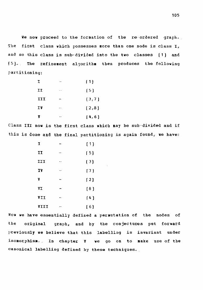
105

We now proceed to the formation of the r~-ordered graphoThe first class which possesses more than one node is class 10

and so this class is sub~'divided into the two classes {1} andf5}o The refinement algorithm then produces the followingpartitioning:

I

IIIIIIVV

r 1}f. 5 1

{3 t 7 }

{ 2 .a J

[4p6}

Class III now is the first class which may be sub~divided and ifthis is done and the final partitioning is again foundo we have~

I [ 1 }

II f 5}

III [ 3}

IV [7 JV f 2}

VI [8 }

VII f q }

VIII { 6}

Now we have essentially defined a permutation of the nodes ofthe original graph8 and by the conjectures put forwardpreviously we believe that this labelling is invariant underisomorphismv In chapter V we go on to make use of thecanonical labelling defined by these techniquesv <

106

JY~~T~Q g~obl~~~~Following on from the definitions made in this sectionp a

number of interesting questions are raised~. Since it isconjectured that two identical representative graphs imply thatthe graphs they represent are isomorphic to one anothero it mustcertainly be possible to reconstruct the original graph (with apossibly different labelling of the nodes) from therepresentative graph~ Actuallyo this is done when there-ordered graph is formede but the refinements which take placeduring the formation of this graph implicitly use the adjacencyrelationships of the original graph. The question of finding analgorithm to build a graph given only its representative graphis then raised.

In the spirit of Ulam~s conjecture (1960) that a graph G isuniquely reconstructable from the set of n subgraphs G - {x} foreach node x in Gp,we pose two further problems:.

(a) is it possible to reconstruct a graph G of n nodesuniquely given only its n vertex quotient graphso and~

(b) is it possible to reconstruct a graph G of n nodesuniquely from its n cycle vectors.

If we vere able to prove the statement made earlier thatpartitioning the nodes by cycle vector or by vertex quotientgraph gives the same partitioning6 then the problems (a) and (b)are equivalent~ Howevero for the moment. ve must leave them asopen questions~ .

107

We set out in this chapter to construct a correspondencebetween the set of non=Ls oeorphLc graphs of n nodes, and theintegers 1Q.a.eg~c where g~ is the number of such graphs •. Onemethod for counting the non-isomorphic graphs is using Polya'stheoremo and it was hoped that this study would lead to a methodwhereby any objects which can be enumerated by using Polyaistheorem may also be systematically generatedtechnique.

using this

However we were only able to reach a partial solution tothis problemu in whichq as we shall showo we are able to set upa systematically ordered list of the graphs of order no but notthe 1-1 correspondence with their counting numbers at which wewere aiming~ That iso we were unable to construct a mappingwhich would take a graph into its index number and vice versa,In fact a number of different lists were formed~

We now consider a graph to be a collection of n pointso andwe may label them in anyone of n¥ ways. For this set of npointso we have n{n-l)/2 positions where a line may be placed.Le, there are n(n-1)/2 possible ways of choosing two points(an unordered pair) from a set of n. Now we may label tbeseline positions according to some rule (we shall discuss someways of labelling the line positions later) 0 and clearly any

108

rermutation of the nodes gives rise to exactly one permutationof the line positions~ Thus we may define an isomorphismbetween the symmetric group of order n (iD~. the group of allpermutations of n objects) and a certain subgroup of thepermutations of order n(n··1)/2,.

Consider now a labelled graph. As we have already notedv

we may define a labelling of the line positions~. A bitstringmay now be used to specify this labelled grapho in which a ioneV

1ndicates the presence of a line in the corresponding lineposition, and a VzeroV bit indicates the absence of a line~ Nowclearly application of one of the permutations in this subgroupof order n(n~1)/2 (which we will denote by L{Pn) ) will permutethe bits within the bitstringn forming a new bitstring". If onebitstring 01. may be permuted into another bitstring f3 using oneof these perautat Lona , then we say t.hat the bitstrings Q{ and ~are equivalent. It is clear that if two bitstrings areequivalent, then the two graphs which they represent are alsoisomorphice since the permutation of the bits which carries

bitstring ~ into bitstrinq f (i"e. a per.mutation of the linepositions) is induced by a permutation of the pointsc and thisis precisely the definition of isomorphism between graphs"

The use of the word ~equivalentn between bitstrings isjustified since it is easy to show that the relation

there exists a permutation in L(P~)mapping « into "is an eguivalence relation bearing in mind that L (Ph) is agroup., Thus the set of all bitstrings is partitioned by this

109

e~uivalence relation into eluivalence classes. each class beinga set of labelled graphs which are isomorphic to one anotherwhen considered as unlabelled graphs~

We now describe the mappings from the point pairs to the

linesa Two such mappings were consideredg and in fact it didnot seem to make much difference which one was usedo

The first mapping was simply to take the point pairs inlexicographic order. and then number the elements of the list

thus obtainedo, Hence. for n = 4" we have~line point··pair1 1

_,2

2 1 ._ 3

3 1 .~ 4

4 2 ,.." 3

5 2 - 4

6 3 .- 4

This mapping has the virtue of being very simple to

implement and to understando

Let us now consider the effect on the line positions of aqraph when the nodes are permuted by the cyclic permutationoUnder this permutation of the nodeso we discover that the linesare also permuted cyclicallyo though not in a single cyclen butin a number of cycleso To give an example of thisc consider thecomplete graph of 5 nodes shown in figo 10 If we now let thenodes lnoa~o5 be permuted cyclicallyo we see that the pair (102)

is mapped into the pair (203) I! (203) into (304) /1 and so on" and

110

also that (1t3) is mapped into (284) etc. In facto as we wouldexpecte if we apply this cyclic permutation 5 tiaeso the graphreturns to its original labelling~ and in doing so the pointpairs (or lines) have gone through a complete cycle of length 5"

However there are 10 lines, which means that the lines must besuch that they can be partitioned into two distinct sets each ofwhich contains 5 lines. These two sets consist of the set of

Ilines which form thereriphery of thediagram, and the set oflines on the interior ofthe fig ure0

In general, for odd values of Dp the lines partitionthemselves into (n"l)12 sets (or cycles) each of length no Foreven values of nv howeverc this does not happeno since the line;oining opposite points of the graph willa after only n/2

applications of the cyclic permutation, finds itself in itsoriginal position (thouqh in the reverse sense)< By opposite

points we mean points iri such that li-jl = n/2e and whichtherefore appear diametrically opposite one another if the graphis drawn with the nodes nu.bered consecutively around theperiphery of the diagram" The same action as for the case wheren is odd takes place for every other line of the graphr Thusthe lines of a graph with an even number of nodes fall inton/2··1cycles of length n and one cycle of length n/20 Thesecond mapping of point pairs into an index number is by thispartitioning 0 and within each cycler by the value of the firstnode" Thus for n = 4 and n = 5 we have~

n = 4 n = 5

line point--pair line point~pair1 1 ~ 2 1 1 .~ 2

1. 2 0- 3 2 2 - 3

3 3 .. 4 3 3 - 4

4 4 - 1 4 4 .~ 5

5 1 .. 3 5 5 """ 1

6 2 -- 4 6 1 ~ 3

7 2 ~ 4

8 3 - 5

9 4 ~ 1

10 5 ~ 2

111

These two mappinqs may be described in terms of fairlysimple functions~

Mapping 1c

line(i,j) = if i>i then line(jr,i)else (i"l) (2n..,i)/2+ j .-L, _

Mapping 2.,

line(iuj) = if i--j>n/2 (mod n) then line (jui)else (j~ i-l) n + L (.-od. n)

where in each case Wline(iui)1 is the line label for the line~oining the points i and j~

In this discussion we have considered the effect of thecyclic permutation of the nodes upon the lines of the completeqraphc It wouldo however" have been egually valid to consider ageneral labelled graph of n nodesu and to observe the effect onthe line positions under a cyclic permutation of the nodeso

112

The problem of findinc;a representa tive of each egui valenceclass in the set of all graphs may now be couched in terms of a\jraphical modeL

Consider the set of all bitstrings of length m = n(n~1)/2uand let each such bitstring be represented by a node in the:;raph modeL Then a directed line is inserted in this graphfrom the node lit to the node f!' it and only if bitstring fti isobtainable from bitstring ~ under the operation of permuting thebits in ~ by one of the permutations in L(P~). Let us define

this graph to be the gg!ti.V:~.~~nQ~ .q!:~.E!lfor the 9raphs of order

Now since for any pair of e~uivalent bitstrings there is apermutation mapping one into the the resulting

eluivalence graph is a collection of connected componentsu eachof which is a complete directed graph., We may also remark thatthe graph may be considered to be undirectedu since whenever aline from node ~ to node ~ exists8 the inverse permutation isrepresented by a line from node ~ to node ~~ If we now take onenode only from each of these connected componentsc this set ofnodes will represent the set of inequivalent bitstrings. andhence we have obtained the set of non-isomorphic graphs.

In order to reduce the number of permutations which have tobe examinedo we require a set of permutations which generate thewhole groupo In terms of the e~uivalence graph modelo this isthe salle as removing lines from the graph but without

113

disconnecting any of the connected components. We know however,from Ledermann (1961) that the two permutations~

(2 3 n 1) and (2 1 3 4 "., n)

will generate the whole of the group of all permutations oforder n, This means that the graph does not lose anyconnectivity by removinq all the lines except those representingthese two permutations.

Let us now consider the action of these two permutations ina slightly different light. Suppose we have a set S of nobjects, and that the objects of S are to be permuted by the tworer'Mutations given" the cyclic perllutation c and thetransposition of the first two elements. Now consider a graphin which the nodes represent the nY ways of ordering theelements of S~ and in which we have two types or ~colours~ ofline, A v bluew line from node Of to node p if ordering (3 isobtained from ordering ~ by application of the first of our twopermutations (the cyclic permutation)u and a ~redi line from ~

to S if ordering 8 is mapped into ordering S on applying thetransposing perll~tationo The graph thus formed is highlysymmetricu and it contains (n-·l)!cycles of length n containingonly iblue' lineso These cycles are not connected to oneanotheru each one corresponding to n applications of the cyclicpermutation. The graph also contains a number of cyclescontaining alternately ~red' and iblueijlines~ These cycles areof length 2(n-1) r which may be seen by considering the action ofapplying the cyclic permutation followed immediately by thetransposition~ This results in the first element remaining inits original positionr with all the other elements being

114

permutations will form arermuted one place cyclically~

cycle consisting of n+ l

'blueu lines and n··1~r:edw Li.ne s , Fig. 2,

shows this graph for thecase when n = 4., Thewbluev lines in fig,Lo are shown as solidlines and the Vred~:linesare dotted "

Thus. n-1 such pairs of

The general problem of scanning all possible results ofapplying any permutation to some object or set of objects is

such as the one in fi9<then a problem of finding a Hamiltonian path through a graph

2. It is not difficult to find a

Hamiltonian path through this grapb when the graph is consideredas undirectede but we must bear in mind that although the ired'lines are essentially non·-directed. the cycles of ~bluev linesare directed so that the cycle is traversed in either theclockwise or the anti'clockwise sense", In the diagram in fig"20 (I this is seen· to be true except that the outside cycle is inthe opposite sense from all the other cycles. This howeverappears guite consistent when we consider projecting thisdiagram onto the surface of a sphereD and then observe thediagram from outside (or inside) the sphere.. The cycles thenare all in the same sense. It appears not to be possible totraverse this diagram~ takin~ due account of the directions onthe lines, so that each point is passed once and once only. It

115

is possible however to find a Hamiltonian cycle if we allow amovement along a line in the 'wrongi direction just twice. Thisis shown in fig. 3.

A graph such as the one in figo shows the

interconnection of the objects when subject to the permutationswhich we have been considering. However, if we consider a graphof n nodes as a bitstring as described earlier~ we may apply thepermutations to this bitstring and we do not necessarily obtaina different bitstring. Thus, for any given bitstringc we mayconstruct a graph such as the permutation graph shownu but inwhich some of the nodes coincide with each othero, This isbecause n! is an upper bound on the number of distinct labelledo

but isomorphic, graphs of n nodes6 whereas in general therewould be less than this number. Let us show this final pointwith respect to an example. Referring forward to list III whichshows the equivalence relations between the graphs of order 4,consider those graphs in the class containing graph

Corresponding to each of these graphs is a node in the ~reducedv

equivalence graph, and from each such node there are two linesla ~redllone and a 'biue~ one, and some of these lines may beloops. The result of tnLs is the.graph shown in figo 4. We

also observe tha·ta surjective mapping is defined from the set

of nodes in the permutation graph shown in fig. 2<>0 onto the

set of nodes in the eguivalence graph shown in figo 4.(. andthat this graph is one of the components of the whole gprunedll

equivalence graph. This component corresponds to the graphs oforder 4 with just one linee

~- 7:

II1)-----: ------~------~------

II,LI

116

r- ,I I

I'- .

Thus we may consider attempting to find theallnon-isomorphic graphs by examining the connected components ofthis grapho A common method of finding the connected componentsof a graph is by finding a spanning forest for the graph. Ifsuch a spanning forest can be foundo then the roots of the trees

connnected componentsoin the forest can be taken as the representatives of the various

A method was devised to carry out essentially theseoperations which discovered all the non~isomorphic graphs of nnodeso The method involved, howevern inspecting each of the 2''''possible bitstrings (where m = n (n'''1}/2) , but it was onlynecessary to look at tva permutationso and not the fullsymmetric group. In common with a number of connected componentfinding algorithmsr we begin by assuming that each node is in acomponent by itselfp and joining components together as soon as

Let us denote the twopermuta tionsa link is discovered between them.

(2 3 4 c <, c n 1) and (2 1 3 4 .<>, n)by A and B respectively., Then ve observe that permutation A

117

lreturns any bitstring to itself after at most n applications.~~'';;.

~i.ilarly B can only te applied oncep since two successive

f~pplications will clearly give the original bistring once more.

'Tn terms of the graph~ there are cycles of length at most n,

representing successive applications of permutation A, and lines

representing the permutation E which have a line in the opposite

direction joining the same nodes, representing a secondapplication of the permutation B. It may be that for some

Dodes, the original bitstring will re-appear after less than n

applications of permutation A~ in which case it is not necessary

to apply this permutation any further to this node.

The following algorithm finds the subsets of equivalent

bitstrings for a given nu and the non-equivalent titstrings are

10und by taking one representative of each subset. Eachbltstring belongs dynamically to a sUbset (represented by a

tree) which includes its known equivalences. The algorithm

~radually merges the subsets leaving finally a collection of

each of which represents a subset of equivalent~'bltstringsg such that two bitstrings appear in the same tree if

end only if they are equivalent. The roots of these trees may

then be taken as the non-equivalent bitstrings.

1. ~ake each node in the equivalence graph the root of a

(trivial) spanning tree by setting below (i) = i for i =0" , 0 c Q 2""-·1• Thus each bitstring is in its own subset 0

2. for each node i, taken in order, which is currently the

root of a spanning tree, apply the permutation A n-1

times or until the bitstring i reappears whichever is

sooner. For each bitstring j (except i) so

118

constructed, set below(j) = i. On completion of thisstepu the distinct trees include those nodes which cante transformed into each other using only (possiblyrepeated applications of) the permutation A. Each tree

now contains at most n nodes •.3. For each bitstring i in orderv apply per.utation B once

to obtain bitstring j. If i = j, then the permutationE has had no effect so ignore this case. If i > j, wemay again disregard the case, since we should

previously have found j such that an application of Bgave the bitstring i. If i < j, then we havediscovered a possible link between two of the treesestablished in step 2. We must first ensure, howeverg

that i and j are in distinct trees, and this may beachieved by inspecting the roots of the treescontaining i and j. (The root of the tree containing

node i may be obtained by applying the function root (i)

which is defined by

root (i) = if below (i) = i then i else

root (below (i» r •If root (i) = root(j} p then the nodes i and j arealready in the same treev and so we disregard this casealso•. If root(i} # root(j), then we need to linktogether the (distinct) trees containg i and j, andthis may be achieved by setting below (root(j» = i.

4. A representative of each subset of equivalent

titstrings is now found by taking the roots of thetrees we have formed, and these bitstrings represent

119

the non-isomorphic graphs of n nodes.

We observe that the action of this algorithm does not give

rise to real spanning trees for the equivalence graphp but we

.ay be ~ure that two nodes are put into the same tree if and

only if they are in the same component of the equivalence graph.

The trees formed are "reachability trees" for the equivalencegraph 0

An example will help to clarify the action of this

algorithm" Assume that n = 4< Then the number of possible line

positions is 60 and there are 26 = 64 possible bitstrings. Wewill denote th·ese by th b s 0 63e num er ~'.'6 • The two permutationsare~

A .. (2 3 4 1)

B ._ (2 1 J 4)

~n this example we use the second mapping from points to lines

and so the permutations A and B correspond to the permutations

(2 3 4 1 6 5) and (1 5 3 6 2 4)

of the line positions respectively.

Step 2 of the algorithm, having set all the nodes to be inseparate connected components~ is to apply permutation A 3

times" or until the original bitstring re-appearso When this

operation is complete the nodes are grouped as shown in list IDList II shows the links that are established by step 3, the

isolated nodes representing the cases where the permutation B

had no effect, and the lines showing the cases where B applied

to i gives j and j > io List III shows the trees as they have

been transformed by the operation of setting below(root(j» = i,

119.

where i ana j are linked in list IT and are at that moment in

different tre8Sc We note in passing that the trees (in list I)

with rcots 3 and 17 become joined by virtue of the link 3 - 17

in list II, and we subsequently discover that there is another

link (from 6 to 20) in list IT which would have connected these

twc treesf but by the time this link was discovered. the two

trees had already been amalgamated. The roots of the trees in

list III are then taken as the bitstring representations of the

non-isomorphic graphs with 4 nodes. and these graphs are shown

in figo 5,

120

0 36 4818(241~: 33

~5049 5238 5619~28

3~: 51~::41

21-42 57

5-10 22~:: 53-58

~4

35 55~:~7 1311 23~:: 59

15 43 63

2.(.-37

16-32 27~::17(: 45

31~4740

o 14--52 31-55

1 15-53 40

2-16 4118

3-17 19 42-56

4 22 43--57

5 23 44

6-20 4524-34

7-21 46-6025~-35

8-32 47-61

9-33 5827-51

10-48 59

11-49 6229-39

12-36 30---"\54 63

13-37

121

o

/,: /69-18~~4

L34 31

17~20

40

5-10-48

7 13-26-37

50

11-49Ls2

",,56

15-53-58

44

22L25

"'35

/462~29-27

43

122

30

4S~5451 60

57

The Isomorphic Subsets of all Graphs of 4 NodesQ

/

47

31 ~2

""55~61

""-59

63

The trees

subsets.indicate the division of the 64 possibilities into 11 disjoint

123

0 0 0 0 0

I0 0 0 0 0

0 1 3

0---0 u0---0

5 7 15

SJ19 22 23

31 63

This algorithm represents a naive approach to the prob~emof generating all the graphs of a given number of nodeso, In theremaining part of this chapter we attempt to improve on thismethodo Clearly this algorithm implies the inspection of most(if ....not all) of the bitstrings in the full set of 2 (where m =0(n--1)/2 )0 In what followso we atte.pt to use certain

124

combinatorial techniques to reduce the number of bitstringswhich need to be examinedo

Harary (1955) shows the method by which we may use PolyaVstheorem to enumerate the equivalence classeso and hence we cancalculate the number of non-isomorphic graphs of n nodes. Wewill paraphrase the arguments usedu and show how PolyaQs theoremoperates in the counting of graphs~ The explanation given byLiu (1968) of PolyaVs theory of counting is used extensively.

In factv the important part of PolyaVs theory is the use ofa

Burnside's theorem which is/~eneral result for enumerating thenumber of equivalence classes into which a given set S is

divided by a permutation group G of permutations operating on So

To reiterateu two members « and ~ of a set S are said to beequivalent if and only if there exists a permutation 9 ~ G suchthat g (tt) = ~o. Then Burnsideus theorem states:Iheoremo-------

The number of equivalence classes into which S is dividedby the group G is

i-\(;\ ,where ~(g) is the number of elements of S which are invariantunder the permutation ga, (ioeo, the number of elements s ~ Ssuch that g(s) = ~.

125

Denote by l{S) the number of permutations in G which leavethe element s invariant~ Then clearly

since theseLuSboth

L ~~J~~Ci

expressions for the total number ofareinvariances over all permutations 9 and all elements so

Now let {~q~,ccooKl be the members of S which lie in oneequivalence c.l.aas , Then for any pair of elements ol. I' (3 (say)o

the number of permutations carrying ~ into ~ is ~(~)c This canbe shown by demonstrating that if g~ is a permutation taking ~into (l (and there must be at least one since ()/.and p are in the

same equivalence class)o then{a} any permutation taking'" into P is of the form g)l.g~

where gL is one of the permutations leaving ~

Lnva rd an t ,

and

(b) for two distinct g., <J. which leave ()(invariant 0 g,..g.:o • ,

and g..gl are distinct permutations taking « into ~ 0

Now any per.utation in G must either leave ~ invariant, orelse it must take ~ into one of the other elements in theequivalence classo Thus the permutations of G can be classifiedinto those that map « into itself, those that map « into ~u etco

Since the number of permutations in each class is Z(<<) u thetotal number of permutations in G is

G = 1. (0() lr noo of elements in thee'l. .. ~,,~le"c. c.J~ss.

126

or

'1. (~) =noo of elements in equivo class

and since this is independent of It l' this must also be the

expression for '(~)6~(~r etco, and hence

L ,,<s) = lGlco.(t I ..;..",I.I.~'(~S

Now summing both sides of this equation over all theeguivalence classesu we have

.Lw,. ~~~) = IG! le no. of equiv , classes. c43u . ~. c.IuSs~nce the left hand side is simply a summation over all sand

So we have

noo of equivo classes = -'L tt(S) =\(\1 SE;S

We have already described the way in which the relevantpermutation group for graphs is constructed from the symmetricgroup of order n~ It is convenient however to divide the set ofgraphs with n nodes into subsets of the graphs with n nodes andP Lines, for p = Oo11/2poc~pn(n-1)/2o, Thuse for the purposes ofapplying Burnside's theorem to this case we have S being the setof bitstrings of length n{n-l)/2 which contain exactly p 'one'bitso In addition we have IGI = n!o,

Making use of the theorem of Burnsideo and particularly ofthe proof, we have6 for any given equivalence class consisting

127

of the elements "-0 (J 0 000 I! I( 8

= 1t-oand since 'l (4() + '1.(~) .. 0 c ~ .. 't(t<.) = nI we know that n!must bedivisible by t(,,)0 Furthermoreg if we can find the permutationswhich leave ~ invariant~ and we can find one permutation mapping

ol into ~ p then we can find all the permutations mapping tJi into flby forming the product g~g. for each g~ ~ II. (where ~ is thegroup of permutations leaving « invariant) 0 Regarding this fromthe other point of viewg we can take any grapho and provided wecan find its automorphism group, we can find all the graphs towhich it is isomorphic by taking each permutation in the set G ~

H~and permuting the graph using this permutationo We can thenfind all the permutations which produce the same graph simply bymultiplying this permutation by all the permutations in H.oWhen this has been performed n!/~(<<) times we know that all thesraphs in the equivalence class containing the graph ~ have beenaccounted forI! and so any graph which does not belong to thisset is a new non-isomorphic grapho

A full set of graphs with n nodes and p lines is obviouslyobtainable by placing the p lines in all possible combinationsin the (~) line positionsp and hence a complete list of all thecombinations of p objects from (;) can be taken as the set ofall graphs with n nodes and p linese. The problem of finding thenon-isomorphic me.bers of this set can now be tackledo Thegeneral approach is to layout the the combinations in a listoand by stages to delete those which are isomorphic to a

128

combination already considered" Thus the method is similar inbroad outline to the method of finding prime numbers known asthe Sieve of Eratosthanesn in which all numbers are laid out ina list, and as soon as a prime is discoveredo the list is passedover once deleting all those numbers which are multiples of thatprimeo When this can no longer be donee all those numbers inthe list which have not been deleted are prime numbers.

We therefore present an algorithm for finding thenon-isomorphic graphs with n nodes and p lineso which will bereferred to as the Sieve algorithm.

1 . ((~») b i ." Set up a bi,t map for the ~ com anat~ons.2. set up a bit map for the n! permutations.3. Look for the first ~setW bit in the map for the

combinations. If there are none, then we have foundall the graphs" otherwise store this graph (as graphW~l say) and ~unseti its bit.

40 Find all the permutations under which graph et. isinvariant (i.eo its automorphism group - cof. chapterIV) and ~unset~ the bits in the permutation bit map

corresponding to these permutations •.Find the first permutation whose bit is Uset'o Ifthere are none~ then go to step 2u otherwise let thispermutation be g~o

6. Apply the permutation g~ to the graph ~ and 'unset' thebit of the resulting graph in the graph bit map.

70 Form the permutation g...g, for each gL E BoO(and ~unset'the corresponding bits in the permutation bitmap,

80 Return to step 5.

129

A few comments on the representations of the variousobjects used must now be given, since both the graphs (whichare mapped onto the combinations of p lines chosen from a set of

(~) ) and the permotations are to have bit maps associated withthem. it is obviously necessary that both the combinations andthe permutations should be readily representable as integers,and more precisely as consecutive integersv That is. for boththe combinations and the permutationso it is important that theconversion from a combination or permutation to itscorresponding integer in some orderingo and vice versa. can beachieved quickly< In the case of permutations, the mostconvenient method appeared to be a slight variation of themethod of Lehmer (1964)0 and this method gives the permutationsin lexicographic ordero

In this methodu it turns out that it is more convenient toconsider the permotations of O.1o.~oon-1 rather than of

1p2uco~on and that the permutations be numbered from 0 up to

n!~1 instead of 1 to n! The method itself is based on the factthat any number in the range 0QO. q un1-1 can be expresseduniquely in the form:

a,,_,(n'~1)i+ a.._~(n-2)X + oqo + a. 11 + aerOXwhere 0 ~ a~ ~ i for each i.

The mapping from the integer k to the k-·th permutation inlexicographic order is then constructed by forming the a~ Vs fork., From these we can construct the permutation by noticing thatthe i-th position is occupied by the a~-th element of thoseremaining at that stage. We can see this rather better by

130

considering an exampleD Suppose we wish to find the 63rdpermutation of the numbers 0,102q3{/4o (remembering that (0 1 2 34) is the O-th) 0 The first step is to put 63 in the form

2c4! + 2031 + L2~ + L1~ + OoO~

Le" = 2 = 2 a~ = 1 a, = 1 a~ = 0 (Notice that ao isalways zero, hy the condition on the a.) 0 The first position inthe perautation is therefore occupied by the element 20 and thesecond position contains the element 2 in the set Ou 1" 30 4

Le. 30 Element 1 of of the set o u 1 o 4 occupies the nextpositionq and element 1 of the set Du 4 is the next member ofthe permutation •. The last position is of course filled by theonly remaining elemento in this case 00 and this is a reflectionof the fact that the value of ao is always zero. Thus the 63rdpermutation of the numbers 0 to 4 is

(2 3 1 4 0)

The reverse mapping is obtained simply by reversing theprocess co.pletelY6 reconstructing the at~s from the permutationand then multiplying out the ~polynomial~ to arrive at theinteger L

Similarly a mapping from the set of integers 10" 0" n (~) tothe set of lexicographically ordered combinations of k objectsfrom a set of n can also be constructed"

With regard to the multiplication of the permutationsy itis clear that the most efficient method of achieving this is tostore the multiplication table of the permutation groupo butthis is obviously impractical since its space requirement is for(n~)2 elementso Thus the multiplication must he carried out

131

directlyo but this can be done reasonably efficiently providedthe mapping from permutation to integer and vice versa isefficient~

The remaining part of the algorithm which needs to bedescribed in more detail is given as step 4 ..- finding the groupot permutations under which the 0raph is invarianto We nowdescribe an extension of Corneilus algorithm for finding theautomorphism partitionin1 of a graph (Corneil 1971) to displaythe automorphism group. The algorithm for obtaining theautomorphism partitioning has already been described in therrevious chaptero and we present here the extension required to,;;eneratethe automorphism qroup,

Suppose we have a 'lraph whose automorphism partiti.oning hasbeen found using the partitioning algorithm" Then we have thenodes grouped together in a number of disjoint setso These sets

were used to form the re-ordered graph of the previous chapterrby selecting one node from any set containing more than onenode. and placing this node in a class by itselfn This newl~rtitioning was then refined using the partitioning algorithm.Now the conjecture is that in the automorphism partitioningc forany pair of nodes within a classo there exists an automorphismmapping one of these nodes into the other. Thus there are IV~Iways of choosing an element from V~o assuming that V~ is thefirst set for which !V~l >,. The refinement then takes place.having made one such choicee and the process is repeated. The

132

total number of automorphisms in the automorphism group is thefroduct of the number of ways in which a choice may be madewhenever a choice is to be made. Hencec if H is theautomorphism group:

where s :.~ is the set of nodeso which after j-1 assignments andthe corresponding refinements of the partitioning. has IV~ I > 1

but 1V\tjl = 1 for k< L

The actualrermuta tions which makeup the automorphism ~ c;O"-------<OO b

qroup can of course befound by actually making

d 0-------(:1 C

all the variousassignments which areavailable at each stageoand then carrying outthe refinement.

An example will show more clearly how this method works.Consider the graph of four nodes shown in fig~ Theautomorphism partitioning is~

Making the first assignment6 we have a choice of four nodes. sowe choose one of theme say a. After applying the finalconnection partitioning algorithm6 the partitioning is!

I {a}

{b}II

133

III

It is apparent that if we now make an assigment to resolve

the difficulty of set III having two nodeso we must make a

choice between these two nodes~, Since (by conjecture at least)

the partitioning would have the same form whichever of the four

nodes an bg c, d were chosen for the first assignment~ we know

that there would always have been a further choice between two

nodes to be madeo Thus the total number of nodes in the

automorphism group is 8 (= 4 X 2)c

To continue with the example, the second assignment

(together with what amounts to a trivial refinement) we have:

I

II

{a}

{b J

{cl

{d}

III

IV

This is the result of choosing c for the set 1110 but we

could equally well have

which results would be:

I

II

III

IV

chosen du in which case the partitioning

{a ]

{b}

[ d}

(c}

Thus we have formed two permutations under which the graph is

invariant and these are;,

(a b Cd)abc d

and ~

134

b Cd)b d c

We may now write down the six remaining permutations whichresult when the other three choices are made at the first stagetogether with the two choices at the second stage in each case~

b c

a c

b c cd)a d

d a

b c

Changing the notation slightlyo so that the nodes a f/ b , cand d are replaced by the nodes 1, 2w 3 and 4 respectivelYb anddenoting a permutation of n numbers 1v2v'''',on by a vector oflength D

135

(pI P Pa. 6 0 0 0 0 p" )where P. is the value of the i-th element after the permutation

has been a pp.Li.e d , we may write dowm the permutations under which

this graph is invariant a ss

i (1 2 3 4)

a (1 2 4 3)

b (2 1 3 4)c (2 1 4 3)

d (3 4 1 2)

e (3 4 2 1)

f (4 3 1 2)

9 (4 3 1. 1)

This collection of permutations can easily be shown to be a

';;roupwith the followinq multiplication table ~

i a b c d e f 9

i i a b c d e f g

a a i c b e a 9 f

b b c i a f 9 d e

c c b a i 9 f e d

d d f e 9 i b a c

e e g a f a c i b

f f a g e b i c a

g 9 e f d c a b i

Throughout this chapter we have been concerned with makinga selection of objects (in this case graphs) from a larger set

of objects such that we have exactly one representative of each

136

e'~iuivalence class in the set under some definition ofequivalence~ To achieve this we require that the set of objectsfrom which the choice is made should contain at least one memberof each eguivalence classu IdeallYe of coursee the set fromwhich we make the selection would consist of exactly the set ofnon-equivalent objectsg in which case the selection mechanismrequired is the trivial one of selecting each object in the set.

Although this was our original aim, we have not been ableto achieve this goalu and so we have taken as our starting setthe set of all bitstrings of length n(n-1)/20 This correspondsto saying that we can take the set of all labelled graphs anddeduce those that are non~isomorphic when considered asunlabelled graphs, We have implicitly recognised however thatno graph with n. nodes can be isomorphic to a graph with n~nodes if n. I n~o The length of the bitstring is then a partialspecification on the set of graphse knowing that all isomorphsmust have the same partial s~ecificationo

We may now consider the possibility of carrying out asimilar process on a set of graphs with a more precise partialspecificationu This stems from the fact that if two graphs areisomorphico and d is the mapping which takes the nodes of onegraph onto the nodes of the otheru ~x = y implies that thedegree of x is equal to the degree of Yu This is true for allnodes x in the first graphe and so the degree sequences of twoisomorphic graphs must be identicalo where we define the Q~g~~

§~g~~~£~ of a graph to be a vectorg = (d I lJ da. 00 u 0. 0 d..)

137

where d' is the degree of the node i (in some labelling) andL

such that d· ~ d~..., for i = 1,,000.n-10 This is also known as~

the £~rt!!!2!! of the grapho Two graphs cannot be isomorphic ifthey have different degree seyuenceso . However" it is not truethat two graphs with the same partition are necessarilyisomorphic" as can be seen by the example given in fig, 7.These two graphs both

have degree sequencehave 5 nodeso and both

(3 2 2 2 1L, but the twographs are clearly notisomorphic" since for to.)instance the node ofdegree 3 is adjacent tothe node of degree 1 in~lraph (a), which is nottrue in graph [b) 0

In the earlier section concerning the Sieve algorithm6 the

total nu.ber of graphs which needed to be considered was n~xg"Owhere g~ is the number of non-isomorphic graphs with n nodes.In fact, this was done by finding a graph topologically distinctfrom any graph previously examinedo and then inspecting each ofthe n1 permutations of the labelso An alternative viewpoint isto consider generating all the labelled graphso and thendiscarding all those which are not already in canonical formeBy this means we would retain only the graphs in canonical formp

so that if two graphs in the set are isomorphicn then they arealso identical" in which case the problem of removing duplicates

138

is made correspondingly easiero

If we could then generate only the set of graphs which arein canonical form alreadyc the starting set of graphs would alsobe much smallero As a first step towards thisc we observe thatthe algorithm for reducinq any graph to its canonical formbegins by classifying the nodes of the graph by degreeo Thuso

in the canonical labelling~ we know that if node i has degreed·

L then d· > d·J - Jt", This is of course simplythe condition on the degree sequence of a graph. so that we mayconsider attempting to generate the set of all non-isomorphicgraphs by examining only those labelled graphs whose labelling~ives rise to a valid partition for the graph. We also noticethat only a restricted number of the n~ possible labellings of agraph give rise to a valid degree sequence for the graph.

We could contemplate generating the set of all graphs bythe following algorithm~

1. Generate all degree se~uences.2. For each degree sequence. generate a set of graphs

which must necessarily contain at least one instance ofeach non-isomorphic graph with that partition~

3" Eliminate duplicates from this set.

Harary (1968) quotes two theorems which give necessary andsufficient conditions for a partition to be the degree sequenceof some graph, and we will make use of both of these in thecourse of implementing this algorithm. The first theoremu dueto Erdos and Gallai (1960) states:

139

A partition (d.pdl,CcCoC od,,)of a number 2m is the degreesequence of some graph if and onll if:

d· ~ r (r"1) .."

min

for each r, 1 ~ r ~ n~ .

We will not give the proof for this theoremo since thestatement of the theorem is sufficient to suggest an algorithmfor generating all the degree sequences for graphs of n nodes.

We begin by observing that the partition (n-1,n-1rnaqun-1)is valid (and corresponds to the complete graph) 0 The algorithmthen uses each degree sequence to generate the next one, theterminating condition being that the elements of the partitionare all zeroo which may be recognised by the appearance of azero as the first element of the partitiono For each iteration

of the main loopu the steps are as follows:

Find the smallest j sote d·J can be reduced without

destroying the ordered nature of the partition Cd; ~

20 Reduce dj by one.Reconstruct the elements dj~ ydJ-J.v 000 od. making surethat the partition always satisfies the condition ofthe theorem 0

4. check that the final sequence is a partition of an evennumbero If sOo then this sequence is the requiredpartition otherwise repeat the steps 1 to 40

140

Step 4 is required since it is possible to construct apartition of an odd number such that all the conditions (exceptthe evenness condition) are satisfied6 but such a partition is

not a valid degree sequencen since~ d. = twice the number of lines in the grapho

(This is easily seen since each line in the graph makes acontribution of 1 to the degree of each of its endpoints. andhence a contribution of 2 to the total sum) 0

The second theorem which Harary quotes concerning thepartition of a graph is due to Hakimi (1962):

A partition

f! = (d. vd1{,,~rcd ...)

of an even number 2m is a valid degree sequence for some graph

if and only if the partition(d'l. -1 o d1 ,. 10<> ~ " 0 d.. .,.1 u d_ +lU ~ c 0 Cld.. )"'.+' ,

is also a valid degree seguence for some graph"

For this theorem we give the proofo as we shall requiresome of the techniques used in the proof later on"

If g' is valide then clearly so is £ since from a graphwith partition g' we may construct a new graph with partition £by adding a new nodee and joining it to the first d, nodes ofthe original graphu where d. is the degree of the new node"

Now suppose that G is a graph with degree seguence du If

141

there is a point in G of degree d, which is joined to nodes ofdegree dl.e c 0 • cd..." then the removal of this node win give a....graph with partition g~o If there is no such pointe then wemust show that from the graph G we may construct a graph GW withthe same partition which does have such a pointm Now in Go nodei has degree d.

I.for i = and d ~ ~ d ~.t for i =

1o.~"on-l0 In particular noue 1 has the largest de9ree~ Now inthe graph we may find points i and j such that d~ > dj and suchthat line (ll,j) is in G but line (1('i)is no t , (If this were

not so, then we would have the situation aboveo where node 1 is~oined to i for i; 20, aocd.+1). But since d~ > ~ 0 there musta node k such that (i6k) is in G but (jok) is noto If we now

remove the lines (1ui) and (iok) and replace them by the lines(1 c i) and Uo k); the new qraph has the same partition QIl but thesum of the degrees of the nodes adjacent to node 1 has increasedby 10 It is now possible to repeat this process untileventually we acquire a graph with the desir.ed propertyo

The proof of this theorem highlights two facts:(a) We have an algorithm for generating one graph with agiven partitionand(b) Any graph having a particular degree sequence can betransfor.ed into a graph with the same degree sequencep butwith the property that the node 1 is joined to the nodes 2,3o.~.,d, +1. and that the degree sequence ordering ismaint ained.

142

Now fact (a) indicates the algorithm to be used to generatea graph with the given partitiono The method is simply to joinnode 1 to each of the nodes 20 3, ••• ud, +1. and then construct a

~;raph with partition {dt.<>16dl·>1ro~.odd.•1 -1cdCll,.~rooood ••.) on thenodes 2woooun.

Fact (b) suggests that since it possible to transform anygraph with this partition into this "standard" formo then it isalso possible to generate any graph with this degree sequencefrom the "standard" graph by an appropriate sequence ofoperations of the type given in the proof of the theorem. Thus.in order to generate the set of all possible graphs with a givendegree sequence. we must use the algorithm suggested above totind one such graphl and then define the set of alltransformations which are the inverses of the transformationsused in the proof of Hakimi~s theorem. Naturallyc in carrying

out these transformations the graphs produced will not all bedistinctt but we may either leave the problem of sifting out theduplica tes to the third step of the generalised aLqorLt.ha , or we

may sift out the duplicates as we proceed.

The algorithm for finding one graph with the givenpartition simply joins node 1 to node i and subtracts one from

d~ u for i = 263 B o 0 00 d,...10 The remaining nodes are then:ce"ordered so that the new partition is still ordered correctly"During this opexa t.Lon , the node LabeLs, which were originally 1/1

200000n in that order. are carried with the new degree values inthe re-ordering process", When this has been doneo the algorithm

/."'. fe~te~ onis/the nodes 20000/ln (re-ordered) according to the revised

143

degree sequenceo

Let us now demonstrate this with an example in which thenumber n of nodes is 6t and the degree sequence

~ = (4 4 3 3 2 2)

this graph will have 9 lines since the sum of the d~ is 18~

The first step is to ~oin node 1 to each of the nodes 2(, 3c..4 and 5" The degree se'luence which results" after re-ordering (/is (3 2 2 2 1) and the new ordering of the nodes is (2 3 4 6 5) 0

If the procedure is repeated8 the node 2 is joined to nodes 3('4

and 6e leaving a partition of (1 1 1 1) and no further:re'~ordering isnecessaryo The nextstep joins nodes 3 and4p and the final stepjoins nodes 5 and 6.The final graph is thengiven in figo 8a

The second algorithmo that which constructs every graphwith the given partLt Lon, is somewhat more complicated 0 Itsaction is to reverse the process which was described in theproof of Hakimivs theoremo In facto ~t is more complex thanHakimiis constructiono since in that case the problem was tomove towards a form of the graph which was in some senseoptLaa L, This constructive method moved through a series ofsteps to achieve its goalo Now for any graph obtained duringthis iterative process8 there are possibly many graphs for whichone step of the iteration would give this grapho and in

144

reversing the processn we are faced with the problem ofidentifying ~1!graphs for which this would be true~

We begin by defining a class of grapbs, which willeventually contain all the graphs we are seeking. Initiallyc itcontains only one graphc the graph constructed by the previousalgorithm. The algorithm then applies a series oftransforllations to each graph in the class in turnu and eachtime a new graph is found, the class is enlarged to include this(;raph. It turns out also to be a convenient stage at which tocheck for duplicationso A new graph is only inserted in theclass if it is not already contained in the classo The way ~hisis checked is to use Corneilvs algorithm (see previous chapter)to reduce each graph to its canonical form (as definedpreviously) before attempting to place the graph in the class.We recall that we conjectured (following Corneil) that two~raphs are isomorphic if and only if their respective canonicalforms are identical, Thus each graph is put into its canonical£01:110 compared with each graph already in the cLaas, and if itis different from each one~ then the class is enlarged toinclude this new graphl which itself now becomes eligible to betransformed.

The transformation algorithm is as follovs~1. Assume that the initial graph is in canonical form as

defined in the previous chapter .. In particular thisimplies that d· ~ d· for i < j.~ J

2,. For each node i in the graph r find nodes j. ko I inthe graph such that i < j < kg i < 1 and such that the

145

lines (iei) and (kol) are in the grapho and the lines(i,k) and (jpl) are not,

3.. Remove the lines (i6 j) (ko I)6 replacing them with thelines (iek) and (j.l)v This step should be repeatedfor each 4·-tuple satisfying the conditions in step 2,

40 Each graph produced in step 3 is put into canonicalforme and compared with each graph in the class. If itis found to be there alreadyo then it is discardedrotherwise it is added to the class.

50 If there are no more graphs in the class to be"developed"w then the algorithm terminates; otherwisethe next graph is chosen from the class and thealgorithm is restarted at step 20

The conditions on the nodes io ju k and 1 as shown in step2 are explained in the tollowing way~

(a) ie need to consider all nodes i in the graph. ratherthan just node 1 as required by Hakimius proof, because thisinterchange of lines may need to be done at a differentstage of the process of deciding whether a partition is aValid degree sequence. HakimiVs proof implicitly takesaccount of this by the fact that his argument is recursive.(b) je k and 1 are all greater than io since for each i weare essentially concerned with the subgraph defined by the

(C) The condition j < k stems from the fact that we knowthat dj ~ db when j < kc and we certainly want to ensurethat this is sou since dj < dllis the condition required forthe transformation in Hakimivs theoremu and we wish to

146

construct the reverse transforma tion..

By examination of several examplesc it is clear that thisalgorithm produces the same graphs a number of times overr andthat the amount of work re~uired in sifting out the duplicategraphs is more than we would wish. It is also regrettable thatsome partitionso for which there is only one grapho will causethis algorithm to look in vain for others. One solution wouldbe to make use of some work of Parthasarathy (1968) which showshow to deterlline the number of non·..isomorphic graphs with aliven partition. If these numbers were also computedc then itwould be necessary to invoke the above algorithm only when a:;:artitionis seen to have more than one graph associated withit. It would also be possible6 and perhaps desirable6 to knowin advance the number of graphs which any partition will yieldrso the algorithm can be stopped as soon as this number of

distinct graphs have been generated.

We conclude this chapter with an example of this algorithmat work. In figo 900 we show the graph of figo 8. labelledas graph A, being a graph with pa rtition (4 4 3 3 2 2)" ,

Alongside we give 8 permissible 4-·tuplesg and the graphs whichare obtained by the application of the transformation defined byeach 4-tuple •. This is done for each graph in the classy andeach tille a new graph is discovered" its canonical form is;laced in the class. The (]raphs A8 Bp et D and E are indeed thecanonical forms of the" 'Jraj,hswith this partition (see Haca.cy1968 Appendix 1),

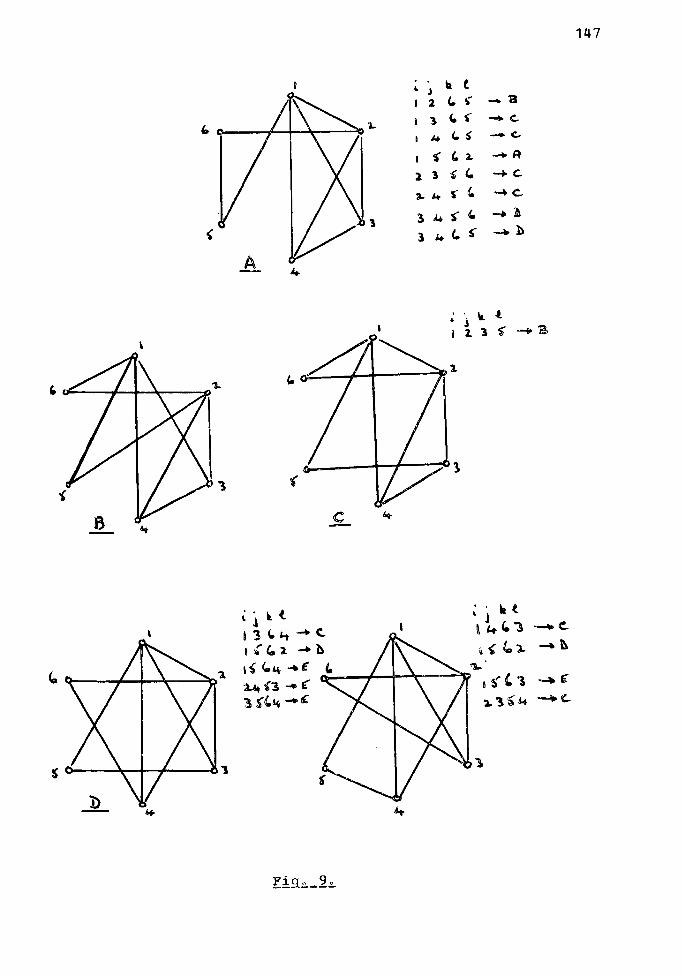
147

. b" ~ tI 2 (. \ _'8

I 3 (. S""_ C-

I 1.+ (.:S"_ c..

I ~ (. ~ -A1 1 ~ (. .....c.~l+S"(. ~c...

3 <4 S"' '"-+)

3 i+ (. S" ..... b

4-

.:l~t13(.",-(.I'"'' ....bI~<'~"'!':I..... i'3 ... ('3 !'-&i - re

~j • ta 1.+ (."3 ..__.~

~"t.~- ~

148

In chapter lIIe we dealt at some length with the problem ofordering and indexing trees of various kinds, and to this endc anumber of ways were discussed for the decomposition of treesinto smaller trees, In some sense this may be described as afactorisation of a treeo This decomposition or factorisation ofa tree is a useful tool in the derivation of recurrencerelations for counting treeso It was considered a naturalextension of this to attempt to use thedecompositione to study the ordering

same technigueo ip~.of qraphs, From the

;Tevious aect.Lon, we see that we can in fact generate graphs insome way by use of the Polya theorem approachu with itsassociated study of permutation groups and similar combinatorialtechniques.

Howeverc factorisation of a graph is a subject of study inits own right and we now discuss some of the concepts involvedin the factorisation of a linear grapho

A !~£!9r of a graph is defined to be any subset of thelines of a graph such that each node is incident to at least oneline in the subset~ Thusn any partial graph of a graph is afact or, An !t:iac!2!:is a factor in which each node is incidentto exactly n lines in the factorp certain particular cases offactors are of interest. A 2-factor is a factor in which eachnode is incident to just two lines - i.~" it consists of a setof disjoint cycles where each node lies on one of the cycles.

149

If a 2-factor consists of just one cycle or componentc it issaid to be a ff~~i11~~i~g £y~1~v The problem of finding a cyclewhich passes through each node of a graph once and once only isknown as Haa.i.Lton v s probLem, and it can be seen immediately thatthis is precisely the problem of finding a 2-factor with justone component. No efficient algorithm is yet known for findinga Hamiltonian cycle of a graph~ or even of deciding whether oneexists, although several theorems have been proved statingnecessary conditions for the existence of such a cycle (see forLn s t anc e, Harary 1968).. Certain heuristic methods can howeverbe used, but these essentially take heuristic ~short cut.sv in analgorithm for solving the problem by exhaustive searcho Berge(1958) describes a method due to Fortet (1959) for solving therroblem for a direct.ed Jraph, but similar techniques do not lendthemselves easily to the solution of the undirected case.

Another type of factorisation which is of interest is the1-factora This is closely related to the subject of matching in

a general graphr, and in factu a perfect matching is a1·factorisation of the qraph.

Berge (1958) defines a mat£~ing M of a graph G to be anysubset of the lines of G in which no two members of M areincident to the same node of Go A !I!!!.!A.!!~!!!!!i£!!.igg_ is amatching M~ for which

IM~I ~ IMI for any matching K of Go

where IMI denotes the number o£ lines in the matching M~ A

150

matching M8 of a graph G is said to be p~~!~£~ if each node of Gis an endpoint of one of the lines of Mo

Clearly if G possesses anumber of nodes in Go must

perfect matchingr then the

be evenr and if M is a perfecta graph has a perfectmatching of Go then IMI If

matchingu then we may attempt to find this matching which coversthe graph by using a backtracking techniguea This can in factbe done recursively by selecting any line of the grapho removingthis lineD its two endpoints and all the lines incident to theseendpoints. We may then examine this reduced graph for a perfectmatching. If it has one, the matching for the whole graph isthe matching for the reduced graph together. with the line whichwas removed initially from the whole graph. If the reduced~raph has no perfect matching8 then we replace the line whichwas removed initially and try to remove a different line fromthe original graph. In facte since each node must be incidentto one line of the matching for the graph to possess a perfectmatchingu it is only necessary to try those lines which are

incident to one node. If none of these yield a solution. thenwe know that this node cannot be covered by a matching line andtherefore no matching found by this method could be a perfectmatching.

For a large graph, howevere this backtracking method willbe extremely inefficient! because of the amount of searchingwhich may be requiredn Given a graph G with a matching Me anode x is said to be £Q~~K~Q by the matching if a line belongingto the matching M is incident to xo The graph G is said to be

151

covered by M if each node in G is covered by Me Any node notcovered by a matching M is said to be !'!YQse!l"1~1h of a graph with respect to a matching M is a pathx, t Xl,l C.e eXit in G in which if line X"_I x, is not in Mo then theline xi,x ':.1 is in PIc Thus an alternating path is a seque nee oflines in the graph which are alternately in M and not in Mc

There is no requirement that this path should be of odd or evenlength, nor do we require that the first line should be in M ornot, However, as can be seen from the following theorem due toBerge (1958)r an alternating path of odd length joining twoexposed nodes is of particular interest~~r.h~Q!:~!!

A matching M of a graph G is maximal if and only if no twodistinct exposed nodes are joined by an alternating path~RIQQ.t;,.

This is not Bergeis proofo but a slightly simpler proof dueto Edmond s (1965) c.

Assume we have two exposed nodes Xi and x1 which are joinedby an alternating path P; Since x I and x1. are exposed N thefirst and last lines in the path must be non··matching lines(Lee lines not in M)e Thus P consists of an odd number oflines and contains one more non-matching line than it doesmatching linese If a new matching is now constructed whichconsists of the non-matching lines of P together with the linesof M which are not in Pg this is clearly a matching M' for which

pp I ::: IMJ + 1

Thus M is not maximal,

152

Now assume that M is not aaxd.aal., L;e~matching M' such that

1M', ~ 1M! + 1

We have to show that there exists an alternating path which

there exists a

:oins two nodes which are exposed relative to M~

Consider a graph G¥ which has the same vertex set as Gc andwhose lines are the lines of G which are in either the matchingM or the matching MW but not both~ No node x € G~ has degreegreater than 2 since at most one line in M and one line in M~ isincident to x~ The connected components of Gij are therefore~

(a) isolated nodese

Ib) alternating cycles relative to H (and to MU)or

(c) alternating paths.(a) and (b) have either no lines or an equal number of linesfrom M and M'. Therefore at least one of the components of type(C) must contain more lines of M' than it does of Mc by the

assumption that IMW! > IMI. The first and last lines of such apath must be in M' and thus the endpoints of this path areexposed with respect to M.

This theorem gives the clue to a better method of finding aperfect matching of a graph. In factu the backtrack proceduredescribed earlier will find a perfect matching if there is one(albeit rather inefficiently}u but says nothing about thematching that is produced if no perfect matching exists.

153

The method suggested by BergeWs theorem is to search for analternating path between any two exposed nodes"is found for any pair of exposed nodes then wetheorem) that the matching we have is maximalperfect if a perfect matching exists)G

If no such pathknow (by the(and therefore

This idea has been modified and developed into a workingalgorithm by Edmonds (1965) and later witzgall and Zahn (1965)added a further modificationo The algorithm is basically aprocedure for growing a certain type of tree from an exposednode in such a way that if at any stage a terminal node of thetree is adjacent to another exposed nodee then we have analternating path from that exposed node to the root of the tree,

Edmonds defines this particular type of tree which he callsan alternating tree, An ~l.tern~tip_qlI~~ is a tree in which thenodes are divided into two classes called i!!!!~! and Q!Lt~£ nodes"Each line in an alternating tree joins an inner node to an outernodee and all the inner nodes have exactly two (outer) nodesadjacent to them" If there are m inner nodes in an alternatingtree. then the tree has 2m lines in ito It follows thereforethat the total number of nodes in the tree is 2m+1o and that thenumber of outer nodes is m+10 Thus there is one more outer nodein an alternating tree than there are inner nodes"

Although we have defined an alternating tree in general-terms" we now go on to describe how we are going to use thenotion of an alternating tree to help to find alternating pathswithin a graph on which a matchin~ is defined.

154

Given a graph G together with a matching M on the grapho wemay consider an alternating tree of which one of the outer nodesis designated as the root of the treeo Now let us grow analternating tree on the graph G so that the root of the tree isan exposed node of G with respect to Ho and that every innernode is joined to one of its neighbours by a line in M, sincethe root is an exposed noder i.eo it is incident to no lines ofM. each inner node which is adjacent to the root is joined toits other neighbour by a matching line. This then de£ines howthe matching lines are to be inserted into the tree" It isclear that in a tree of this sarto only the root can be anexposed node of Gl' since if one of the outer nodes is found tobe an exposed node of Gr we have found an alternating path tothe r oo+, and the matching M of G may be enlarged as describedin the proof of the theorem~ Edmonds describes such a tree as a

.r:l!!.l!.t~Q tree L but in view of our previous use of this term o itwas felt that the term ~~!£hing!,~~would be more appropriate.

The growing of a matching tree within a graph G from anexposed node r with respect to a matching H is in fact a way offinding all the alternating paths from re and as soon as one ofthese alternating paths meets another exposed noden we have whatis known as an ~.~SL!!~!!!:in.gp.~!:h for the matching M in G,

In a matchin9 tree rooted at a point ru all the outer nodescorrespond to nodes which may be reached in the tree from r byan alternating path of even lengtho. Similarly. the inner nodesare those nodes for which no alternating path of even lengthfrom r existse but only a path of odd lengtho We therefore

155

prefer to rename the outer and inner nodes of the matching treeas ~~~n and 2££ nodes respectively.

Let us clarify these points using an example. Consider the';raphshown in f Lq , 10 This graph has associated with it amatching and the lines in the matching are marked in the figure.Node 1 is an exposed node with respect to this matching and so~e may look for an augmenting path from node 1 to anotherexposed node in the graph. We therefore grow an alternatingtree from node 1 as shown in fig. 2. Now in this treec nodes1, 56 11" 16, 30 8(, 14 and 9 are even nodes, and 20 120 151J 40

6~ 13 and 10 are odd nodes. Now node 8 is adjacent to node 7which is also an exposed node. Thus we have found an augmentingpath

(1,,2uSl,6,,8l'7)

and this in turn allows us to increase the matching by removingthe lines (205) and (6c8) from the matching and replacing themwith the lines (102) 0 (5l.6) and (7178). We also observe that ifthis change is made to the matchingu the new matching is now;)erfect ,

156

The object of Edmonds~ algorithm is to find all those nodesx in G with the matching E such that there is an alternatingrath of even length from some exposed node ro From this we mayeither find an augmentins path and hence increase the matchingy

or establish that there is no such pathp and hence that thematching is already maximalc A detailed description of Edmondsv

algorithm follows~ .

Starting at the rootr we search for any point x which isnot exposed, and which is adjacent to the root r. (If there isa node y. adjacent to re which is exposed. we may immediately2ut the line (y,r) into the matching). The node x is then putinto the tree~ and becomes an odd node. The node z such that(xyz) E l! is also put into the tree and z is an even node, Allthe even nodes in the tree are then developed in this wayu Fora typical even node p being developed, we find a node x adjacentto p. We now have four cases to consider:

(i) x is an exposed node" In this easel! an alternatingpath from x through p to r has been foundo and theappropriate changes may be made to the matchingo

(ii) x is not exposedc and has not previously been put intothe tree, We now take the step described earlier.calling x an odd nodec and z (where (XIZ) C M) an evennode.

(iii) x is in the tree already and is an odd node. Noaction is taken in this case"

(iv) x is already in the tree and x is an even nodeu Thisis the most interesting case. since this defines acycle of odd length in the graph. We know that p and x

157

both have even length paths to L Define the node b tobe that node which is common to both the path from p tor and the path from x to rw and such that the path fromb to r is of maximum lengtha This is the point atwhich the two paths from x to r and from p to r meet.and it may indeed be the rooto Now b is an even nodeo

since either it is the root itself 0 which is even bydefinitionn or else it has three lines incident to itp

the lines in the paths from b to the r oo t , p and x

respectivelyo Thus since odd nodes have exactly twolines incident to them we conclude that b must be aneven nodeo Thus by discovering a line from p to Xc wehave established an odd cycle in the graph consistingof the two paths b to p and b to Xu both of which areof odd length. and the line (Pwx). Edmonds calls this

odd cycle a Q1Q§AQ~o

If a blossom has been found in a grapho we mayconsider any node c within the blossomo If c is an

even node in the path from p to bu then c is even withrespect to the root , If c is odd in the path froll p tobq since we have an odd cycle passing through Pr bn X

and Co there is an even length path c to p to x to b.Thus c is again even with respect to the root by virtueof this path through x, Hence within a blossoml/ everynode can be considered to be even a Thus the t.reegrowing can be continued now considering the blossom asa single even vertexEdmonds) 0

158

Witzgall and Zahn (1965) describe a very slight variationot Edmondsw algorithm in which the action taken on recognising ablossom is a little differento In this methodw a tree (which

may be called the gveg R~1h i~e~below(i) = j

if and only if there exists a node k with the lines (ivk) and(k,j) in G, such that (ie k) f£ M and (k•.j) / M 0 The step taken

is built in which

when an x is found not in the alternating tree is as beforer andhas the effect of adding the node z to the even path tree sothat

below{z) = pIf an odd cycle is encountered in which p and x are the extremesof two even paths, and the line (XII p) is found to be in G 6 thealgori thm of witzgall and Zahn then chains down the path from pto the rootw adding the odd vertices in this path to the evenpath tree as ~abovas" of x, and chains down the path from x tothe rootw adding the odd vertices in this path to the tree aswabovesv of po If in the chaining down process two adjacent

even nodes are foundn then this implies that an odd cycleinvolving these two nodes has previously been foundo and so thechaining process stops 0 If the node b is the point at which thepaths p to r and x to r meet as defined before v the chaininqprocess also stops when b is reachede since any point below b isnot in the odd cycleo "

The algorithm stops if all the even nodes are found to bein state (iii), iv~o all their neighbours are odd nodes (exceptfor members of a blossom). Edmonds calls an alternating tree

159

with this property a Bu~g~±~~~ ~~~~c This may occur before allthe nodes of G have been examinedo This is overcome by removingthe Hungarian treer together with all the lines incident tonodes in the Hungarian treee from the graph Go The algorithm isthen repeated on the reduced ']raph< Edmonds and Witzgall andZahn present proofs that their respective algorithms end withmaximal matchLnqs,

Consider the graph shown in figoThe following example shows the operation of the algorithm"

300 in which the matchinglines have been markedn We see that node I is an exposed nodein the grapho In fact it is the only exposed node in the graphq

but this does not affectthe performance of thealgorithmo Thus I

becomes the root of the A

alternating t r ee, Wefirst grow towards No

(The stages in the c,

development of the treeare illustrated in fig"4) 0

o I (...v« .. )

(b)

r: (odct \

(A&C)' ) (&.... "ec(e" .... )

)

'I(c..,,« '" )

(e)

160

~~-OJC(~01~ .. )

. bl..w)A(.." c.", )

- - - - - - - - - "(en,,)

It 118c..ht') rc; ) "-vc. ..}~~(e..." ...)

(g)

Fig 0 4" (a) -. (c) show how the normal growth of the tree takes

place, and a further extension occurs in (d)o Two even nodes CAand D) are now found to be adjacento. This blossom can now becontracted into the pseudo+ver+ex (ABCDE) 0 In (e) another

growth takes place and again two even nodes (G and the

pseudo-'vertex (ABCDE) ) are found to be adjacento The blossom

again shrinks into a new pseudo-vertex ((ABCDE) FG)" Thispseudo-·vertex cannot now be developed any further n and so (f)shows that further development of 1 is the only chanGe ofgrowing the tree any more" In (g) one further step has beentaken, and this tree is in fact Hungariano If we now remove·this tree from the original graph we obtain the subqraph whichis shown in fig" 50. This subgraph possesses a perfect matchingalready, and hence we conclude that there is no alternating path

161

between any pair of exposed nodes6 and that the matching asshown in figo 3< is maximalc This description only discussesthe final stage of thealgorithm; previousstages have alreadyfound augmenting pathsand modified thematching accordinglyo Pi c 5.~-g--,.-~-

A slight extension to Edmonds~ algorithm has also beenconsideredo This is to grow alternating trees from each of theexposed nodes of the graph. The conditions under which the

"loin" of two trees occurs determines whether an alternatingrath between the roots of any two trees exists.

BrieflY6 we label all the exposed nodes as even nodesp andgrow alternating trees for each one as described earlier, Theaction to be taken in each of the possible cases is as beforeo

except in case (iv)p when two even nodes are to be joined o (If

we previously asked the question Wwas a particular node in thetree'?W we must now ask ~is the node in any tree?W)" In case(iv) however we have to subdivide this occu~rence into twofUrther parts - when the two even nodes are in the same tree,and when they are in different treesc If the two even nodes arein the same treep then they must be treated in the same way asbeforep namelyo the process of reducing a blossom to apseudo-vertex must be carried outu If the two even nodes are indifferent treeso we have then found an augmenting path betweenthe roots of the two trees" This is of course the even length

162

[ath from each rooto together with the line between the two evennodes which are the growing points, This extension to themethod of Edmonds is probably only a marginal improvement overthe original algorithm6 if any.

The study of factorisation or decomposition of graphs wouldnot be complete without a mention of articulation points. Wemake one remark about articulation points in connection with thestudy of aa tc hLnq s , A node x of the graph G is said to be an~£1!9!lati.Q'!!.Eoi.!!! of G if the subgraph G f x } is notconnected, although G is connected •. Berge ( 1958) states andproves the following theorem! which we give here without proof 0

:thgQgU!

A node x is an articulation point of a connected graph Gp

if and only if there exist two nodes p and g in G such thatevery path from p to ~ passes through Xn ,

Let x be an articulation point of the graph Go and letGn.G~8 •••• G~ be the connected components of the graph G { x } •

We define p to be the Q~~~£ of the articulation point x (and wenote that p ~ 2 by definition of an articulation point). Thesubgraphs Go. '" {x} for i = 102(oo~op are called Q!o~~§" It canbe seen that G has a perfect matching if and only if Gj U {x}

has a perfect matching for some j, and G·.. (i j) all haveperfect matchings. A necessary condition for a graph G topossess a perfect matching is that IGI is even. and therefore wehave~

163

ofIf G is a connected graphc and x is an

order p which divides G into blocksarticula tion point

G: u {x} for i =1pO<08P, then a necessary condition for G to have a perfectmatching is

and

IGtl is even for all i # j~

Thus, if a graph can be found to possess articulationpointsu then our backtracking algorithm for finding a perfectmatching may be simplified by associating each articulation

faint with a particular block (according to the rule given inthe above theorem)p and then looking for perfect matchings ineach of the resulting subgraphs separately". It is clearp

howeverQ that Edmondsi algorithm is much more efficient than thebacktracking algorithmo and will cope with articulation pointswithout further modificatione as indeed the example shownearlier demonstra teso

Articulation points are useful in other cases of graphmanipulationQ and so it is perhaps worth discussing a method offinding the articulation points of a grapho

We statedo without proofo a theorem of Bergen which gave anecessary and sufficient condition that a point x should be anarticulation point, Let a ~E~~n~ng!£~~for a graph G be a treewith the vertex set of G, In other wordso a spanning tree is atree which covers the nodes of Go In any treeu there is exactly

164

one path between any two nodes of the treeq and if the tree is aspanning treeD then there is exactly one path in the treebetween any two nodes of the graph. Now if a node x is anarticulation poLnt , t hen, by the theorem quoted above, thereexist two nodes p and ~ such that every path from p to g passesthrough X6 and in particular the path in the spanning treepasses through x. This implies that if a node y ~ G is aterminal node in any spannin~ tree of Go then y cannot be anarticulation point of G. In particularc if we are able to grow

a planted spanning tree (planted tree as defined in chapter Inot Edmonds' definition) from y which covers Gp then y cannot bean articulation point of G, To find the artiCUlation points ofa graph G then we may attempt to grow a planted spanning treefrom each point of Gr and those nodes for which we do notsucceed are taken to be the artiCUlation points of the graph.It is also true that for any tree that is grown I' all theterminal nodes as well as the root can be marked asnon"'articulation pointsu so it is not necessary to grow planted

spanning trees from every node in the grapho It is necessarYrthoughu to grow a tree from each node which subsequently turns

out to be an articulation pointQ ,

It was felt that if some control were exercised over theway in which the tree was grownu it ought to be possible toreduce the number of points from which trees had to be grown.This could be done by attempting to grow a Vbushy~ treeu i.~. atree with as many terminals as possible. Howeverq it turned outthat if a tree-growing algorithm was used which tried to dothisu nearly all the eliminatable nodes were eliminated in the

165

first few treesp and all the subseguent trees had roughly thesame set of nodes as their terminal nodeso

A slight extension to this algorithm can be used to findthe articulation points of a graph. and at the same time findthe order of the articulation pointo (We may perhaps consider anonO"articulation point as an articulation point with order 1)0

Suppose we are trying to find the order of a point xo Weconstruct a spanning tree whose root is Xp and in which all thenodes adjacent to node x are inserted at level'o These nodesare then labelled from 1 to d(x)o indicating that at this stageof growing the treer the node x appears to be an articulationroint of order d(x) 0 As each node in the spanning tree isdeveloped we have two cases to consider. Suppose we aredeveloping node i8 and we find that node i is adjacent to node~ in the graph. Let the label of node i be l(i) 0 Now either~

(i) j is not in the tree. In this case. place j in the tree(by setting below(j) = i or some other.means) and set

l(j) = I (i) o

(ii) j is in the tree. This means that we have found aconnection between the block containing i and theblock containing io If lei) = l{j) then do nothing;otherwise set the labels of all the nodes whose labelsare either l(i) or l(j) to be egual to the smaller of1(L) and 1tj) c

When all the nodes have been developed in this waYr we havein fact inspected all the lines in the grapho and the number ofdistinct labels on the nodes adjacent to x is the order of the

166

node xo If this number is greater than 1r then x is anarticulation point of this order.

We have briefly touched on the subject of growing spanningtrees of various sorts for a given graphc This section isdevoted to an examination of the spanning trees of a graphc andvarious ways of finding a spanning tree.

Obruca (1966) makes extensive use of the spanning tree inthe various techniques he develops v but in his case most of the~raphs are cost associated, and the extraction of a particularspanning tree is correspondingly easier •.

In chapter III~ we described various methods of indexing atree, and in each case we considered the tree as being acomposition of two or more partsv usually smaller trees. Ouriirst approaches to the problem of indexing linear graphs werebased on attempts to decompose a graph in a similar fashion •. Totake an example of this, we defined the natural ordering fort~ees as T < T~c in terms of the ordering of the components T.and T: ' where the tree T is considered to be decomposable asshown in fig, 6. If a

and failed tocomparison between T,

discriminate between thetwo treest'then the twosubtrees T2,and T~ wereexaadned, and so on, g!g.".~.§~

167

In Snow and Scolns (1969) we outlined a similar techniquefor indexing graphso It was pointed out in that paper that alarge part of the problem was the difficulty of decomposing the';raphuniguely < The work of Cornei L, as described in chapterIV. has now removed this difficulty (subject to the conjectures'1'iven in that chapter) r and so the problem of deciding the truthor falsity of the statement G < G' is now theoretically solved~For Lnst anoe, the two graphs could be reduced to theirrespective canonical formsr and a straighforward comparison ofthese graphs such as the comparison of their adjacency matriceswould give the required resulto We have however developed a

number of technigues for the practical decomposition of gr.aphs"

The first problem which was mentioned in Snow and Scoins(1969) was that of finding the centre of a graph. Howeverrthose nodes which map onto node I of the representative graphmay be considered to be the centres of the grapho and since weknow that these nodes form a transitive subgrapho anyone of

these may be taken as the (unique) centre of the qraph, Thedegr.ee partitioning was used as the basis for all therartitionings in the formation of the representative graphe andtherefore the use of the Cayley ordering is suggested fordeciding which spanning tree is to be regarded as the ~best'spanning tree for a particular graph •. Spanning trees of a graphare essentially free treeso and it is therefore necessary totake SOle point in the tree as the rooto. A better choice is tochoose the root of the spanning tree by virtue of its status inthe graph rather than by virtue of its status in the tree

168

(although we would hope that they are connected when we come tocreate the tree), since we already know that the representative~jraphand the re'ordered qraph are invaria nt under isomorphism D

any algorithm will suffice to produce a unique spanning tree fora graph provided it is based on the labelling of the re·ordered~;raph, We haven hovever, made an attempt to find an "opt.LaaL ~spanning tree for a graph, where optimal was taken to be avariety of propertiesu but mainly the property of ~comingearliest in the natural ordering of treesVc As we saw in

chapter 1110 we can equate the ordering which we have called thenatural ordering with the ordering defined by the

lexicographical ordering of the height vectorsn and it is withthis in mind that we attempt to find the VoptimalV spanning tree

for a qraph,

Given any qraphu we may compute from its adjacency matrix.

another matrix6 the shortest distance matrix

whereS = fd ~j )

is the length of the shortest path in the graph from

node i to node jn Furtherp we define (following Obruca 1966) a

m~§h~QQ~ing §~~n~~ng 1r~~ as any spanning tree in which thelength of the path from any node x to the root of the tree isthe same as the length ot the shortest path within the graphbetween the saae two nodes. Now since the height vector of atree is simply an ordered list of the distances from the root toeach node of the treee it is clear that the heightrepresentation of any mushrooming spanning tree will be simply are-ordering of the elements of the row in the shortest distancematrix corresponding to the root. Although we have been unable

169

to prove the statement, it seems intuitively reasonable that ifthe optimal s pan n Ln q tree is defined in terms of the naturalordering of the trees(! and therefore of the heightrepresentationp then the optimal spanning tree will be amushrooming one , The trees which come first in the naturalordering are those with the smaller numbers i.n theircorresponding height vectorsn and the mushrooming tree is alsoan attempt to keep the height vector values as small aspossible~

Two main algorithms were used in an attempt to discover theoptimal spanning tree for a graph, and certain variations werealso incorporated in certain cases. Unfortuna tely it was not0enerally possible to determine whether a tree was in fact theoptimal spanning tree when either algorithm had discovered itoThe two algorithms are slightly different in approach; the firstbeing an iterative methode known as the Improvement Algorithm.

and the second being a more direct methodo

The I.provement Algorithm begins by taking any mushroomingtree of the graph. This may be constructed in a number of waysrof which the simplest is to grow from the root all the nodes ata distance 1 from the roota Then from each of these nodes aregrown all the nodes at a distance 1 away which have not alreadybeen put into the treeo This process is repeatedv building upthe tree by v levelsw r and a mushrooming tree certainly results,Clearly the tree which results is, however. highly dependent on

170

the original labelling of the grapho

Given any spanning tree of a graphp we define the graphwhich results when all the spanning tree lines are removed to be

the £2~tr~~. It is obviously possible to create a list of thelines in the co-tree. The algorithm now proceeds as follows:

Consider any line in the co-tree which joins the nodes xand yo Since the spanning tree is mushrooming v we know that forany such nodes, Ih (x) ..h (y) I ~ L This is because if two nodes

are joined in a qraph, there exists a pa th from some point r tox which passes through Ye and y is the last node on this pathbefore reaching x, thus d (rl'Y)~ d (rex) + 10 Now if a spanningtree exists which does not contain the line (x,y) II then both thepath from r (the root of the tree) to x through Yv and the pathfrom r through x to y must exist. Thus d (rpy) ..1 ~ d (rex) ~

c. (rlly) + 1" and d (rox) --1 $ d (ruY) ~ d (rex) + 1.

The improvement algorithm attempts to replace lines in thespanning tree by lines from the co-tree to see whether a bettertree is formedo This is done by successively trying eachco tree line and removing one of the lines in the spanning tree.If at any stage an improvement is madec then this is adopted asthe new spanning tree and the algori thllrestarted" When eachline in the co--tree has been triedu and no improvement has beenmadell then the algorithm terminateso This method may be thoughtof as a kind of whil~·climbing' technique in which the steplength is one line~ There is clearly a great danger of a vloealoptimullV being found which can only be overcome by replacing twoor more lines in the tree simultaneously, This is an obvious

171

extension which could be made to the algorithm"

In factp this particular method in which the spanning treeis changed as soon as an improvement is made is only one of anumber of possibilities,. An alternative strategy would be tomake all permissible chan~es to the tree,.and select that which..Lves the greatest improvemento This means that the methodwould be a sort of isteepest ascent~ method.

Apart from the extension mentioned abovev there are otherextensions which may also be consideredo For any spanning treen

we may form a certain number of different spanning treesdepending on the lines in the co-treen. The algorithm abovetakes the first of these to be found which is an improved treeu

and the previous tree is immediately discarded, The alternativemethod is to take all the trees given by substitution of oneline and choosing the best of them, We may however considereach of these trees which represents an improvementp developingeach in turn~ and seeing which one leads to the best tree by a

sequence of one line replacementso

Such a process could be restricted so that each stepforward leads to an improved tree. or perhaps so that each stepforward leads either to an improved tree or an egui valent tree.In the limitp the method could develop every new tree that wasfound. in which case the algorithm would generate all themushrooming trees which span the graph" These last methods areclearly using a backtrack type algorithm"

Since the algorithm as it stands begins with a mushrooming

172

spanning treen and stays within the set of mushrooming treesc wemay make some remarks about the choice of lines to be insertedinto or removed from the current best spanning treeu First.assume that we have a line (x.y) in the co-treeu Suppose thatwithin the spanning tree h(x) = hey) 6 iceo in the graph d(xor)= d(10r) where r is the root of the tree (and perhaps the centreof the graph) 0 Then this line need not be considered as acandidate for inclusion since if it were put into the treeeeat her h' (x) = h~{y) .t- 1 or hiey) = hV(x) + 1 (where hU(x) is

the height of the point X in the new tree)o This thereforecontradicts the assumption that the tree is mushroomingo We nowknow that the only lines which we need to consider inserting arethose for which Ihex) - hey) I = 10 We may assume, without lossofgeneralitYnthatd(rex) +1 = o(r['y), Thus we have thesituation as shown in fig•. 7. Now by inserting a single linein a treer we create one simple cycleo It is now necessary toremove one line from this cycle in order to make this graph intoa tree again. The proposition is that the only line which maybe removed so that the mnshrooming property is preserved is theline (Yoz)6 where z = below(y) 0 For consider the removal of anyother line in the path from y to the rooto Then the node zwould be connected to the root only by a path passing through yand x (in that order) u In the mushrooming tree. since z -below(y), we have h(z) = h(y) - 1. Howeverv in the new tree,the path from z to the root is through Yu and therefore h(z) >h(y) u Hence the mushrooming property is destroyedo Similarlywe can argue that no line in the path from x to the root may beremoved and the tree remain mushrooming. The task of testing

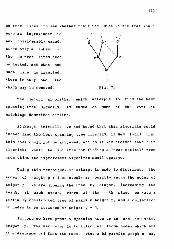
173

co tree lines to see whether their inclusion in the tree wouldmake an improvement isnow considerably easedo

since only a subset ofthe co-tree lines needbe tested, and when onesuch line is insertedc

there is only one linewhich may be removedo

The second algorithmr which attempts to find the bestspanning tree directlYr is based on some of the work onmatchings described earlier~

Although initially ve had hoped that this algorithm wouldindeed find the best spanning tree directlyv it was found thatthis goal could not be achieved I' and so it was decided that thisalgorithm would be suitable for finding a 'near optimalQ treeUpon which the improvement algorithm could operateo

Using this technique~ an attempt is made to distribute thenodes of height p + 1 as evenly as possible among the nodes ofheight po We are groving the tree by stagesu increasing theheight at each st.a qe, where at the p,th stage ve have apartially constructed tree of maximum height Pe and a collectionof nodes to be attached at height p + 1.

Suppose we have grown a spanning tree up to and includingheight po The next step is to attach all those nodes which areat a distance p+1 from the rooto Thus a hi-partite graph B may

174

be defined in which the two sets of nodes are respectively theset of nodes at height p (already in the tree) and the set ofnodes at a distance p+l from the root. Let these two sets be s~

and Sr.' respec ti.veLy, Now if x ~ Sp and y ~ St+\ {, there 1S aline in B if and only if there is a line (xcy) in G. The<;eneral method adopted to distribute the nodes of height p.1 asevenly as possible amon~st the nodes of height p is to assignone node from S~..., to each node in S~u as far as this is

the assigned nodes:ossibleo and when this has been donee allare removed from Sp~1 and the process repeated. Thus we alloweach node at level p to acsuire at most one node from the set ofnodes at level p+l before any node is allowed to acquire a

second node from Sp~l~

It is obviously desirable to assign as many nodes from S p~1

to nodes from S~ as possibler subject to the restriction that nomore than one level p+1 node is to be assigned to any level pnode at each stePe and this problem is then simply the problemof finding a maximal matching on the hi-partite graph Bn

In section 1102 we described Edmondsw algorithm for findinga maximal matching on a general qraph, Howeveru we may simplifythis algorithm when looking for a maximal matching on abi-partite graph by observing that in a bi-partite graph everycycle is of even length. Thus in the description of the actionsto be taken when growing an alternating tree from an exposednode. cases (i)e (ii) and (iii) are exactly as before [but case(iv) cannot occur6 since this would imply the presence of an oddcycle in the grapho which is impossible in a bi'partite graph.

175

Thus we may find a maximal matching on B by growing analternating tree from each exposed node in S and altering therna tching until it is maximal.

Having found a maximal matching on Bp we now attach these

nodes in S" ..., to their corresponding nodes in S tot' so that if x ~S .. and II. (x) is that node in S,"+I such that (xom (x) is a line inthe matchingr the spanning tree of G is enlarged by setting

below (m (x) = xand the node m{x) and all its incident lines are deleted fromthe graph B. When this has been done for each line in thematching6 a new maximal matchin9 is found on the reduced graphB~ and more nodes can then be inserted into the spanning treecThis process is continued until all the elements of Sp~i havebeen placed in the spanning tree~

In passinge we observe that the method of growing analternating tree on a bi'partite graph may be used to prove by agraph theoretic method a theorem due to Philip Hall (1935) known

as the theorem of Distinct Representatives.

Assume we have a set of objects Sf' and n subsets s~ (i =1on",un) of S. We assume that the union of the subsets S·.. isthe whole set S•. Then ve have a set of distinct representativesif one element a~ c S~ can be found for each in such that at =aj if and only if i The element a·"

may be said torepresent the subset S&" Then Hall" s theorem states~~hgQ£~~

The subsets i = 1q<~.on of a set S possess a set of

176

distinct representatives if and only if each set of k of thesubsets has at least k distinct elementso

No~ let each subset Si be represented by a node x ~ X in ahi-partite graph Biland let each element in S be represented bya node y ~ Y of B< Then the lines of B represent the setinclusion of the elements of S in the subsets S~o i.eo Bcontains the line if and only if the element of S

represented by Y is contained in the subset of S represented byx, Now for any subset A of nodes of Xv let rCA) be the set ofnodes y which are adjacent to at least one node in A.may restate the theorem of Hall as~

Zh~QK~!

Then we

For a bi-partite graph B~ there exists a matching whichcovers X if and only if for any subset A ~ X

Ir(A) I ~ lAI

Clearly if we have a matching ft which covers XQ then forany suhset A of Xc rCA) must contain at least those points y ~ Ysuch that (xu y) E ~ for each x E A~ Hence Ir(A)! ~ iA10

Now suppose ,rCA), ~ IAI for each subset A ~ Xp and supposethat we have a matching" which does not cover X. Then there isa node rex which is exposed with respect to ~~ Now constructan alternating tree as follows. Let r be the root of the treeand join to r all those nodes in Y which are adjacent to r.(There must be at leas·tone since Ir({r}) I ~ I{rll = 1)0 If anyof these nodes are exposed~ then we may immediately increase the

177

matching by including the line joining r to this noderOtherwise, include in the alternating tree those nodes y~ ~ y

which are adjacent to rr and the nodes of x which are joined tothe y~ by a matching line~ We may continue adding y nodes andtheir matched x nodes to the tree until either~

(i) we include an unmatched y node in the tree; this nowgives an augmenting path from r to this unmatched ynodev and the matching may be enlarged by one line asbefore.

(ii) no new nodes can be included in the tree, In thiscasec we have some number of y nodes in the tree andfor each of these there is a matching x node. Thetotal set of x nodes in the tree is therefore the setof the matching nodes together with the node ro Thusthe set of x nodes in the tree has one more elementthan the set of y nodes and hence the assumption that

InA) I ~ IAl is contradicted for this subset A of X.

If case (i) occurs. the process is then repeated until all

the nodes of X are matched. Thus if IrCA) I ~ IAI for everysubset A ~ X we can construct a matching which covers Xo

Q" 1::. n,

since the method of qrowing the spanning tree tor a graphexpands the tree level by levele and makes no reference to theprevious structure of the treeo it is clear thatcounter-examples can be constructed to disprove the conjecturethat trees constructed by this method are optimal spanningtreesp but in many cases this does seem to be truer and in the

178

cases where it is notp it appears that the tree constructed by

this method is ~close~ to the optimum in some senseQ Thus itwould seem to be a ~ood starting tree from which to apply theimprovement algorithm. It is also possible to modify thealgorithm to take account of the counter-examples which havebeen founde but unless a general method can be found which canbe proved to workp it is felt that piecemeal alterations willonly push the point of failure of the algorithm backl ratherthan eliminate it altogether.

In the final section of Snow and Scoins (1969) a ratherdifferent approach to the problem of the optimal spanning treewas hinted at. It was observed that if the best spanning treeis a mushrooming treer then its height vector is simply are·-ordering of any vector representing the distances from theroot of the tree to every other node in the grapht i.eo theappropriate row of the shortest distance matrix So Now clearlyit is possible to take such a vector and rearrange it in such away that it is bound to be optimaL It is not then certainhowever that this re--ordered vector represents a spanning treeof the grapho Thus it should be possible to move from theoptimal re-ordering of this vector until a vector is found forwhich a corresponding tree does exist as a spanning tree. Inthis way we could be sure that the tree found was in factoptimalo In a vaYn this ~s rather like the dual approach to alinear programming problem in which we either start with afeasible solution and try to make it optimal also( or else webegin with a solutionwhich is constrained to

179

be optimal, but whichlies outside thefeasible regionp and ,...qradually change thesolution until it isalso feasible.

We shall show an example of a graph with these threemethods operating upon it~ The graph to be considered is shownin fig. 8. Let us assume that the initial mushrooming spanningtree is that shown in fig~ 9{a). This is clearly a function ofboth the labelling of the graphe and the algorithm used toconstruct the tree. For the purposes of this examplec anymushrooming spanning tree would be suitable and the tree in fig.9(a) is just one of these,this tree is::

o 1 233 1 232 121 1 1

The height vector representation of

and the labelling of the tree is shown in the diagram, Thelines in the co-tree are:

1 " 2 0 1 'I 1 (I 1 - 12 II 2 ~. 3 p 3 ~. 4 0 4 .. 5 t'

6 .. 9" 7 88 7 .. 90 8 .-. 90 8 14" 13 ~> 14,

180

,0(a)

10

(b) (c)

Of these only four lines, 1 - 128 7 - 90 8 9 and 13 14

satisfy the requirement that hex) = h(y) + 1~. By trying toinsert the line 1 - 12 into the tree we find that the line to beremoved is 11 - 12. If this is done the tree which results hasthe same height vector as the original tree" and therefore theprevious spanning tree is retained~. The next co-tree line whichcan be tried is the line "7 • 9~ If this is done the line to beremoved is 6 - 7" and the resulting tree is shown in fig~. 9{b) c

This tree has height vector ~

o 1 2 3 2 3 1.2 3 1 2 1 1 1which is less than the previous height vector according to ourearlier definitions. The list of lines in the co-tree is nowrecomputed, and in fact it is the same list as before exceptthatthe line 7 - 9 is replaced by the line 6 The wholelist is scanned again and now we see that the line 1 .. 12 can beinserted to make an improvement. This time the line 11 .. 12 isto be removedu and if this is done. the resulting tree is asshown in figo 9(c) and this tree has height vector

o 1 232 123 123 1 1 1

181

This turns out to be the final tree, as each of the new co-treelines are tried but without any improvement in the spanningtreeo

In the example shown herer it is relatively easy to verifyby inspection that no better spanning tree can be found,However we are unable to say that this algorithm will alwaysrroduce an optimal spanning treen unless the algorithm isextended to produce ~11spanning trees of the graph and selectthe best,

Let us now consider the action of the matching algorithm onthe same graphc. We have assumed in the previous example thatnode 10 is to be regarded as the centreu since it has degree 60

which is greater than the de~ree of any other node in the graphcThus the partitioning algorithm will put node 10 into class Ie

and the centre of the graph may be selected on this basis. Nowthere are 6 nodes adjacent to node 10 and they are nodes 16 20

36 40 5 and 110 These nodes can be attached immediately to node10 which has already been designated as the root of the spanningtree~ We can now look at the sets of nodes at a distance 2 fromnode 10u which are connected to nodes at a distance 1,

1 [12013}

2 Z3 .RI

4 e:5 [ 6 }

11 {9u12}

These connectivity relations are displayed by the

182

bi-partite graph in figo 100 and ve see that a maximalmatching may be found containing the lines (1&12)e (506) and(11r9). The nodes 12e 6 and 9 are then attached to the spanningtree and removed from the bi-partite graphv A maximal matchingon the reducedbi-'partite graphcontains the one line(lc13) and so the node13 is inserted in thespanning tree vith node 0 0 0

'.a,.. 1 .... 01

1 as its below. ri!h_~_lQ.'l...At the second level the graving points are the nodes 128 130 6

and 9w and the corresponding sets of the level 3 nodes are:;12 { 14 )

13 ( 14 )

6 [7oB}

9 {7oB)

Node 14 is attached tonode 12e 7 to 60 and 8

to 9t" and the final tree ,~is as shovn in fig. 1L

It will be observed thatthis tree has the sameheight seguence as thetree shown in figQ 9 (c)although the labelling '+

Gois dLf f e ce n t , r.ig_~_._11~..

Finally we examine the row of the matrix S which

183

corresponds to the node 10. This is~1 1 1 1 1 2 3 3 2 0 1 2 2 3

The optimum way in which this can be arranged into a validheight sequence is~

0 1 2 3 1 2 3 1 2 3 1 2 1 1

but unfortunately this cannot be fitted to any spanning tree ofthe graph. This seJuence may be constructed by distributing theelements with value p+1 evenly amongst the elements with value pconsistent with the sequence remaining a valid height seguencenThe problem comes when we attempt to discover whether aparticular sequence has a corresponding spanning tree in thegraph. This can be achieved by considering all possibleassignments of nodes at a particular distance from the root tothe elements of the vector with that value. Howevero this couldinVOlve a considerable amount of workv and thus it cannot be

This optimal sequence canconsidered as a practical method.however be thought of as a 'lower boundu on the possiblespanning trees8 and as such may be used to restrict thesearching done by the improvement algorithm. The next smallestvector which can be constructed from the tenth row of theshortest distance matrix is:.

o 1 232 123 123 1 1 1which is the same as the height vector for each of the twoprevious optimum trees~ It is now a matter of making anassignment to the values in this height vector so that it

represents a real spanninq tree in the graph" In fact we havealready seen that there are at least two trees which satisfythese requirements.

184

A rooted tree may be considered as a representation of ahierarchyo It is therefore not surprising that thedecomposition operations discussed earlier in this thesis shoulddisplay an hierarchical or recursive structureo By contrastp agraph is essentially nono~hierarchical and non=r ecursIve in therepresentations so far consideredo This section is intended toinvestigate the possibilities of representing a graph by somehierarchical structureo The general approach is to decomposethe graph (which we assume to be connected) by some convenientruleo and continue the decomposition recursively on thecomponent parts. The representation takes the form of a tree inWhich each node is labelled to indicate the exact form of thedecomposit.Lon ,

The decomposition operation is the operation of removing a

spanning tree as described in the previous sectionsv and thisSpanning tree will then be used as the label representing thedecomposition. The connected components of the co~tree are eachtreated as a separate connected graph and are decomposedsimilarly. In factQ the methods of extracting the optimalspanning tree described here ensure that the co--tree isdisconnected. since all the lines from the root are put into thespanning treee and the root itself is left as an isolated nodein the co--treeo This gives rise to the concept of a _§..t!:.l!£!:.!!!:g~~~ for a graph. The graph is decomposed into a spanning treeand a c~-treeo The root of the structure tree represents thisdecompOsition. and the spanning tree which is extracted is used

185

as the label for the root of the structure tree, The root ofthe structure tree has m nodes above itv where m is the numberof connected components in the co-tree~ If any component is anisolated point~ the corresponding node of the structure tree isnot developedo otherwise this node is the root of the structuretree for this component~ Thus we arrive at a structure tree inwhich each internal node is labelled with a spanning tree" andeach terminal node represents a single node of the ori9inalqraphu

An example will help to show how the structure tree isformedo By some means. we find the centre of the graphv andthen some algorithm such as one of the algorithms describedearlier is applied to find a spanning tree. Let us consider thedecomposition of the graph G shown in fig. 120 and the firstspanning tree is illustrated in fig•. 13. Let us refer to thistree as the tree Tp and let the co-tree be the graph C as shownin figol~. The tree T now labels the structure treep and sinceC has two connected componentse there are two nodes in thestructure tree above the rooto The node 3 of the original graphis an isola ted node in Cc and therefore it requires no furtherdecomposi tLon, Hence it also corresponds to a terminal node inthe structure treeo The other connected component of theco+t r-e e C can now be decomposed in the same waYn and theresultant spanning tree T, (j and the coo-tree Cl are shown in

15 and 16 respectively< C, now consists of 5 connectedcomponents6 of which 3 are single nodesr and the other two areeach trees with one line and two nodes. The structure tree S isnow of the form shown in figa lap where the internal nodes are

186

labelled with the tree

Ta T. T.. and T~ 6 .here '1l'

these latter two are

shown in figo 17..,. ana

the terminal noJ.es of S

are labelled with the ,node labels of the

original graph Go f!g~,_11~

""s' 1

3Fig~_1.1~ !':ig~_.1~~

10

[1..,

4p r0

< 01

I fFig~_l2.~ !':ig~~J.E?~

187

'r[ 1: 11

1.

E!g_:: __17.lC.

Thus we completely represent the process of decomposing a~;raphby its correspondiny structure tree, Having decomposed asraph into its structure tree~ we would like to make thisprocess reversible6 i.e. from the structure tree with its nodelabels can we reconstruct the original graph? Clearly this canbe done if the node labels of the graph are kept in eachspanning tree as well as at the terminals of the structure tree"The guestion then is: How much of this information can be

discarded such that the reconstruction can be done unambiguously

and successfully? This is stiLl an open questd.on, but we maymake some observations which allow us to reduce the ambiguitieswhich are present with the information which is available"Firstly. since the extraction of the spanning tree implies thatall the 1il1es incident to the root of the spanning tree are putint.o the spanning tree. we know that there must be at least oneisolated node at each level of the structure tree. and the rootof the spanning tree which labels each non-terminal node of thestructure tree corresponds to one of the isolated points of theco+t ree associated with that spanning tree c,

188

The second observation which can be made is to do with thepoints which may legitimately be joined. Consider the graph Gshown earlier, in which an attempt is made to reconstruct the~raph corresponding to the spanning tree T and its associatedco·treeo Now by the way in which it was constructed we knowthat T. is mushrooming with respect to the graph which it spans"and the two lines that form T~ and T} join nodes x and y forwhich Ih ,(x) ~ h, (y), ~ 1 where h, (x) is the height of the nodex in the tree T.. However. even after applying this restrictionon the graph we still have a choice of how to compose this graphwith the tree T and we conclude that the str.ucture tree aloneis not sufficient to specify a graphfurther information must also be carried.

completelyp but someAs has been pointed

out previouslYr to carry the node labels of the graph is clearlysufficient~ but considerably more than is necessary. Thus someintermediate quantity of information must be carried, but it isnot immediately clear how much"

Some remarks may be made about the strueture tree however1. The total number of terminal nodes in the structure

tree is equal to the number of nodes in the graph"2" The number of lines in the graph is also represented in

the structure tree. By remark 10 we know that thenumber of nodes in a tree which labels a node x of thestructure tree is n(x)6 where nex) is the number ofterminals of the structure tree which are contained inthe subtree whose root is x. Thus the number of linesin the tree which labels x is n{x) 1. Hence [l thegraph which is represented by this subtree of the

189

structure tree is composed of the graphs represented bythe principal subtrees standing on Xr and the treewhich labels x 0 Thus it 1~ (i::: 1. 0 ~ 0 0 k) are the nodesahove Xc and wex) is the number of lines in the graphrepresented by the subtree standing on X6 we have± w(Yd + n t x) - 1w ( x) :::

.:...We also have

n (x) :::It.L n (y; )

~7:'and for each terminal node t in the structure tree I'

n (t) ::.:'I t: wet) :-"00

Thus we may evaluate n(x) and w(x) for each node x inthe structure tree, and the number of nodes and linesof the decomposed qraph are given by n er) and w (r)respectively where r is the root of the structure tree

of the decomposition.

It is clear from the fact that any spanning tree of a graphwith n nodes has n..1 lines, and from the way in which the

structure tree is bui Lt, that the more lines there are in anysubgraph, the taller will be the corresponding portion of thestructure treeo For instance, if the graph to be decomposed hasonly n-1 lines (the minimum number which it can have withoutbecoming disconnected) it is itself its own spanning tree o andso the structure tree i.sthe tree of height 1 with n+1 nodes,the root being labelled with the spanning tree which is thewhole graph. On the other hand, if we look at the structuretree for the complete graph of order ne we see that the onlymushrooming spanning tree of this graph is the tree of height 1with n nodes, and the co-tree consists of the root of this

190

spanning tree as an isolated nodew together with the completejraph of order n-1" Hence the structure tree would be as shown

The structure

in fig. 19, where the

Tlo are the labels ofthe non-terminal nodesand the label T.., is thetree of height 1 with i

tree in this case has

By application of the formula for the number of lines in theqraph corresponding to this tree we have~

w (r) = w (ur (r») + n 1

= w (ur (u r (r)») .~ (n - 1) --1 + n - 1

= w (ur(ur(r)»).. (n - 2) + (n < 1)

= 1 + 2 .; "c <. + (n _. 2) + (n .> 1)

= n (n ~. 1)/2

which is indeed the number of lines in the complete graph of nnod e s. (In the formula we denote the non-terminal node aboveand to the right of node i by ur(i)o

This observation sU9~.ieststhat we may be able to use thenotion of the structure tree to investigate graphs for highlyconnected regions and in particular to look for completesubgraphs sometimes known as £lig~~§". Such an investigationdeserves separate st.udy , and is outside the scope of the presentwork,

191

A complete study of the properties of the structure treehas not been attempted. but it is felt that it is at least apossibility for further work in the study of representations ofqraphs, which field currently lacks a truly recursive andhierarchical representation" A further advantage which mayresult from such a study is the ability to apply our techniquesfor describing trees in a labelling independent way to the moregeneral problem of the description of an unlabelled graph"

192

In the precedin:l sections we have discussed methods whichare applicable to certain problems connected with the generationor the decomposition of trees and graphs. All of the algorithmsdescribed previously have been coded in the Algol W language(see Wirth and Hoare 1966) for the IBM 360/67 computer. In thefollowing sections we describe some of the practical details ofthe coding and give some indication of the size of problem thatmay reasonably be tackled using these technigues.

Under this heading we describe the two methods of orderingthe set of trees as described in chapter IIIv In particular wediscuss the methods based on the two main representationsemployed. ,

As was pointed out earlier" the heigh t representation didnot allow us to solve the problem of finding the k-th tree inthis set without storing the whole table of numbers of trees byheight and number of nodes as given by Riordan (1960) (see alsoAppendix I) 0 However" a program was written which successfullygenerated the whole sequence of trees of a particular size bygenerating each tree from its predecessoro the first beingsupplied explicitly., The first program written to perform thistask took a very simplified viewv by taking the first treev

Le" the tree with height sequence

193

o 1 1 one 1

and successively attempting to increase each element in t urn,beginning with the last elemento subject to the constraint thatno element may exceed its predecessor by more than oner andsubject also to the constraint that the whole sequence must be avalid height sequence" This, like the method described in Snow(1966)u was inefficient in the sense that a number of completesequences were generated and subsequently rejectede. Thus thetime required to generate all the rooted trees was more nearlyrelated to the number of ordered rooted trees than to the number

of unordered rooted trees"

In Scoins (1968)0 howevero a very elegant recursive methodof producing the list of all rooted trees of n nodes ispresented. The heart of this method is a recursive procedurewhich determines the upper limit of any element in the heightvector by keeping a record of the element with which the current

element is to be compared. Thus a backward pointer is kept for

each element indicating the subtree and the node which limit thevalue of that element if the sequence is to satisfy theconditions of the canonical ordering" The Algol stack mechanismtakes the responsibility for maintaining the list of backwardpointers upon which this method relies" By keeping such a stackit is possible to generate the height vectors of all rootedtrees with a given number of nodes without duplications, andwithout either generating any sequences which have subseguentlyto be rejected or requiring any complicated checking process toensure the validity of any sequence producedn Thus using thismethode the time taken to generate all the trees is much more

194

closely related to the number of rooted treesp i.e.t.akenper tree is more riearLy constant"

the time

A program was written to discover the k,th tree with nnodes for any nr and any ko 1 ~ k ~ T~ in the Cayley (weightr:epresentation) orne rLn.r [ but since to some extent this involvedcounting up through the trees with partitions less t.hanthepartition of the k~thc it is not a fair comparison to generatethe k-th tree for each k ::= l~G.<cT", and compare this method witha technigue in which each tree is generated from itspredecessor. This is because in generating the (t+1) th treec alarge amount of work already done in finding the k..th tree isrepeated. However this methode it is claimed. has a differentfunction from that of generating all trees of a certain size andis therefore to be considered on its own merits.

We recall that the weight representation uses the number ofnodes in a subtree (or the VweightV of a subtree) to describethe node at the root of each subtreeo and that for a tree with nnodes. the weights of the nodes adjacent to the root form apartition of n-l. This was discussed in section 11103.2

The program discovers first the partition of the k·-th tree II

by inspecting each partition in turn and asking how many treesthere are with this partition. and subtracting this value fromk. When the value of k finally becomes negative we know thatthe current partition is the partition corresponding to therequired tree u and that we rer]uire the k v . th tree with this

195

j.artLt.Lon, where kllis the last value taken by k before becomingnegative, The next step is to set up a vector kd(i) i =

In •• cop where p is the number of parts in the partition for therequired treep and where kd{i) is the index number of the treeof size part(i). This tree may then be found recursively foreach ie and the weight representations of these trees may beinserted into the appropriate positions in the weight vector toobtain a complete representation of the k<>thtree with n nodesin the Cayley orderiny.

The problem of generating all trees in the Cayley orderingrdisregarding the problem of generating the k~·th t.ree, is

somewhat more akin to the problem of generating the last (Th-th)such tree by the method described above. This is because it wasfound necessary to wcount through 1/ all the other trees i.ntheset in order to find the lastc and the action of actuallygenerating them on the way past is a relatively small amount ofadditional work.

The comments made here about the amount of work required bythese various methods are summarised in table Iv in whichprograms An Band C are respectively Scoinsu method forgenerating trees by height se~uenceo the method which finds thek-th tree for k = 180.~oT~p and the method which generates theT~' th treen but is extended to display the other trees~incidentally' 0 The programs were all written in Algol Wandthe figures are seconds of 360/67 CPU time.

196

n I ProgoA ProgoS progoC

5 0005 0010 0,,04

6 0010 0031 0,,12

7 0,,23 1,13 0040

8 0<~3 4011 'I"039 1039 15052 2076

10 :3081 60"76 7 ,,65

Some indication of the time requirements for Corneil~salgorithm as described in chapter IV are given in the finalchapter of Corneil~s thesis (Corneil 1968), in which he claimslhat the isomorphism algorithm which he describes has a running

time proportional to n' where n is the number of nodes in thegraphso and k is related to the highest level of strongregularity of any subgraph in the qrapha, and that if the graphsare no more than 2'~stron9ly regularv then k = 50 This is a

significant improvement over previous graph isomorphism

algorithms, for which the worst case running time wouldapparently be proportional to ni for a pair of n node graphsoCorneil deals in some detail with the establishment of timingestimates for all his algorithms and examines the performance ofhis isomorphism algorithm on a series of special classes ofqraphs, such as polygons and generalisations of polygons 0 Healso shows that his estimated results agree ~ery closely with

197

the observed timings. Another observation made by Corneil isthat his observed results suggest that most pairs of graphs canbe tested for isomorphism in a time considerably less than theupper bound of n5r and in general the time required isproportional to about n3~

The whole of Corneilus algorithm has been recoded in AlgolWand tested on a number of trial graphsc It has not beenrossible to perfarm a satisfactory series of tests on theperformance of this algorithmr since this should be done by

generating a large number of random graphs with n nodes andtaking the average time for the execution of this algorithm forvarious values of nD The disadvantage of this method is a lackof understanding of what is meant by randomness in graphso Avery crude method would be to generate random upper triangularbinary matrices with various controllable parametersr such asthe number of nodes nr and the density (the proportion of cones~

in the matrix). This methode howeveru does not allow anycontrol over the structural properties of the graph. We areunable even to guarantee connectedness (or otherwise) of the~raphs produced by this method. The algorithm was howevertested on a sample of graphs of various sizes and all that canbe said is that our observations agreed to a significant extentwith those of Corneil and with his theoretical predictions,

The algorithms developed to generate graphs. discussed inchapter V. were somewhat disappointing in their performancer in

198

the sense that the generation of any graphs with more than about8 nodes seemed to be quite impractical by these methods"However, it must be pointed out that this is at least in part

due to the explosion of the number of graphs to be generated~ Amore meaningful measure would perhaps be the rate of generationot the graphs. that isp the time per graph taken by a particularalgorithllo

In spite of the fact that the sieve algorithm was able touse the canonical ordering algorithm to determine theautomorphism partitioning and hence the automorphism grouPe itstill turned out to be necessary to obtain every permutation inthe set of n! for each distinct graph generated~. Thus it wasnecessary to generate a total of n~.g~ permutations. where 9A isthe number of graphs with n nodes. This method could only bejustified if the cost of applying a particular permutation to agraph is significantly more than the cost of mUltiplyingpermutations. This is clearly not true in the representationswhich have been chosen herep and we conclude by saying that nloperations (in this case permutation multiplications) per graphis unacceptably high. Beside this figureo the additionalrequirement of (say) nS for discovering the automorphism groupof each graph may be regarded as negligible.

Before we discuss the efficiency or otherwise of the

199

equivalence graph method of genera ting all the graphs of n

nodeso it is appropriate to digress a little~ and look at the

asymptotic behaviour of the se~uence g~ for n = 1c 2.

From the work at Harary (1955) and also Davis (1953) we

have an expression for 4ft:

..1 L 2,Hx>If\1 ~c: ....

g.. =where d~) is given by

d (;r;:) - ~ PII. {[ k/2] + k (p~ ,1) ) +

where (h , k) is

L p._ PIL (huk)\,..cd.

highest common factor of hand k, and thethe

cycle class of the permutation x is given by {PI (J PL.Q 0 o " I. P..) o

The minimum value of a (Je) is taken for any cyclic permutation o

where the cycle class is (OoOyoo~e1)o In this ca se ,

cl (~) == [n/2 J

Thusr gR is a sum of n~ terms each of which is not less than[ ...h.l

2 Into Hence

Similarlyo the largest value of a{~ appears when ~ is the

identity pe rau tatLon , whose cycle class is (n[lOq"9000)0 In this

case

1husu by a similar argument to that given aboveo..(..- .,'~g"" s 2

This is in fact only a confirmation of the fact that there

are fewer unlabelled graphs than there are labelled graphsu

whichp as we saw in chapter Ve can be represented by the set ofbitstrings of length n (n·-1)/20

200

It is clear6 howeverr that the number of graphs is relatedin some way to 2~ where

n/2 ~ k ~ n(n-l)/2

2 '" ('" - I) I'LThe number of nodes in the e(luivalence graph is andthe number of connected components is gh which is proportionalto some power of 2a It is therefore clear that while the sizeof the equivalence graph is growing faster with n than is thenumber of connected componentsp the difference in rates ofqrowth is not as marked in this case as it was in the case ofthe sieve algorithm. As for the program to find these graphs,it was felt that the number of permutation applications requiredto establish the connectivity of the equivalence graph was afair measure of the work required to obtain the set of graphsQIt was observed in the examrles tried that the number of suchapplications required a~peared to be approximately proportionalto the number of nodes in the equivalence graphc the constant of

proportionality being about lD~~

The largest value of n for which graphs were actually~enerated was 60 There were two reasons why no more wereattempted 0

(a) this took 90 secsa of CPU timep and it was estimatedthat n = 7 would require 90 minutesa

(b) the space reguirement for representing the eguivalencegraph was causing a problem, since the graph for n = 7would have 221 nodes.

201

In this section there are two distinct aspects to consideroFirstlYe it is necessary to generate all the graphical[artitions of length no and secondly. the set of graphs withthis partition has to be completely generated. The algorithmsunder discussion here are described in section V~5.

As regards the set of graphical partitionsp it is expectedthat the time taken to generate a single partition from i t.S

predecessor would be proportional to no In factp the algorithm,in broad outlineo scans along a partition looking for an element

to reduce8 and haviny found onen it moves back to the beginningof the partition recomputin9 all the earlier elements" Thus wemay expect to have to recompute on average one half of theelements at each stage~ In any case the recomputation requiredis proportional t.o n, Actually~ as t.ableII shows, the timerequired per seguence seems to be proportional to some power of

n which is slightly greater than onee This can perhaps beexplained by observin q that the algorithm actually generatessome partitions of 2~~ numbers which satisfy the criteriap andthese of course have to be discarded as non-graphicaL In termsof feasibility" however, we see that we can generate all thegraphical partitions of length 9 in only 30 secso and thus it is..uite practicable to generate these and possibly also those oflength 10 and 110

202

n no, of time time/seq

sequences (secs) (ms/seq)

4 11 0006 5045

5 31 0016 5016

6 102 0053 5020

7 342 1086 5044

8 1223 7042 6007

9 44S0 34078 7<82

The creation of an initial graph with a given partition is

trivial, particularly if the adjacency ma trix is used to

represent the grapho The generation of all graphs with a given

partition is however a completely unknown quantity as far as any

analytic treatment is concernedo All tha t is possible at

present is to quote some experimental observa t.Lon s,

We saw in the example at the end of chapter V that there

were a total of 18 different 4~tuples to be inspectedp whereas

the number of graphs which were actually produced was 5. and one

of these was found directly.

We present here some general remarks related to the

performance of the various factorisation techniques described inthe preceding chaptero As in section Vllo2e these techniquesare highly dependent upon the actual structure of the graphr and

203

it is therefore necessary to perform a series of testsF applyingthe algorithms to a large number of randomly generated graphs.A~lainwe must remark that the subject of randomness in graphs isnot well understoodp and thus such tests are of limited valueonly c.

Edmonds sugyests that his method operated in timerroportional to n. for finding a maximal matching on a graph ofn node.s, His argument was based on some very generalised

o~V'&ti ..."statements about the maximum number of times a particular/can becarried OUtD and how many operations are involved in theseoperationso Now while Edmonds~ estimate is only presented as anupper bound on the methodl we claim that it is far from being aprecise upper bound~ For instanceu Edmonds remarks that thematching can be found by growing an alternating tree from at

most n points, and the alternating tree algorithm requires timeproportional to n3 to find an augmenting path and amend theaa tch Ln q, Apart from the trivial observation that only n/2trees are requiredr since each improvement in the matchingincludes two further nodese we also observe that in at least ODecase, and except for very special graphs in other cases as wellu

the operation of finding an au~menting path is simply that offinding a node adjacent to the root of the alternating treeDwhich is an order n operation at most.. This case arises whenthe matching is empty. i.ee when the first alternating tree isbeing qrovn,

204

The method of backtracking to find a perfect matchingp incommon with most backtrack type algorithms can be unpredictablewith regard to its re~uirements, In the best possiblesituation, as would be the case in (say) the complete graphp ar-erfect matching can be found in as few as n/2 attempts (wherean attempt is to be thouqht of as removing a line and itsend-points from the graph)c whereas in general it would be moredifficult than thiso In the worst caseo and this includes allthose cases where the algorithm fails to find a perfectmatching, the work done will be nearer n~ than no This method,as was noted earlier" also has the disadvantage of failingcompletely when no perfect matching exists, while on the otherbandr Edmonds' algorithm will always find a maximal matching.whether this is perfect OJ:' not ,.

Yl1.!.2 Articulation Points.- -_ ~___________ _ __ ,_ ~L.~~

The most efficient spanning tree finding algortihm will intheory operate in time proportional to mu the number of lines inthe graph, but in practice this is probably more like nZ formost implementable algorithmso This we will use as the startingpoint for our discussions.

The articulation point algorithm as described in thepreceding chapter will reyuire an amount of work proportional ton"tt where ~ is the work required to find a spanning ·treein agraph. This is an upper bound. since we need to grow at mostone spanning tree for each node. We notice in passing that theoperat.ion of growing a planted spanning tree is no d.ifferent

205

from growing any other type of spanning treeo The slight savingto be made by marking all the terminal nodes of any spanningt.r ee, so that no spanning tree is required from these nodes,will only make a difference of an approximately constant factorin the time of operation of the algorithm. This factor appearsto be around 2/3. but is of course dependent on the actual graphbeing considered.

The time ~ to grow a spanning tree on a graph is of coursethe time required to grow a labelling dependent treep and thealgorit.has described in section VI. 4 require more operationsthan those required for any spanning tree. In the first placera mushrooming tree requires more work than a general tree. withregard to the improvement algorithmc although the number ofchoices of lines which are candidates for insertion is much

smaller than the total number of lines in the co··tree0 and oncea choice has been madep the line to be removed from the tree iscompletely determined, there seems to be no way of predictingthe number of iterations which may be carried out by thealgorithmo

The matching method for constructing the first mushroomingspanning tree is of course trading time to set up this tree for(hopefully) a saving in the number of iterations of theimprovement algorithm. No detailed comparisons have beencarried outo but preliminary observations suggest that a smallamount can be saved by combining these two algorithms,.. Some

206

more concrete results on the extraction of spanning trees from agraph are reported in Chase (1970)~

The complete decomposition of a graphc and the constructionof a structure tree is simply a repeated application of thespanning tree algorithms described earliero One decomposition~s required for each internal node of the structure treer andthe number of these is related in some way to mr the number oflines in the original grapho A first estimate of the workrequired to perform the complete decomposition of a graph wouldthen be .'t'o

The somewhat imprecise remarks made above about theperformance of the algorithms described under the general titleof Factorisation are included to illustrate two main facts~.

(i) Considerably more effort is required to understand morefully what is meant by vrandomnessu in graphsr, and theWexpected~ performance of an algorithm operating on a'typical' grapho.

(ii) All of these algorithms vork in time proportional tosome pover of no where this power is fairly smallaThis means thatc inrequired by any ofembarrassingly great8

generalr the amount of timethese algorithms will not beand that any graph which can be

fitted the main store of a modern computer can be

207

processed in a reasonable timen This is in contrast tothe methods (such as those described in chapter V)where the number of entities (eog. graphs) is

explodin 9 as n inereases, and aI though the objects maybe quite small in themselvesu the number of them[ andhence the time resuirect to generate them all~ isincreasing in an unmanageable way,.

In this final section we attempt to make some remarks aboutwhat has been achieved in the worko and to draw together all thefinal remarks whicb can be made about the work as a wholeo Inaddition we wish to point to further problems and investigationsalong tbe same lines which we feel it would be profitable andinteresting to pursue ,

In the tree section there is not a great deal to say..

Clearly we have not exhausted the possibilities for representingtrees, but we have been successful in that the tworepresentations on which we have been concentrating ourattentions have both yielded reasonably satisfactory methods ofgenerating trees. the second of which the weightrepresentation relates this generation very closely to onemethod of counting trees,

It is unfortunater but seemingly unavoidableu that the two

the t.re e s , as displayed byThe natural

the heightrepresenta tionsordering of

are to some extent in conflict.

representation, is more closely related to the structure of the

208

tree than is the weight representation I' but the weightrepresentation is bound to be more related to the countingsequences because these latter are always expressed in terms ofnumbers of nodesc A radically different approach to thecounting problem could perhaps reconcile these tworepresentations.

with regard to the graph isomorphism problem. we raised two-iue stLons related in detail to the work of that chapter c namely"the reconstruction of a qraph given only its cycle vectors orits vertex quotient graphs. A more general problem might beattacked using some modifications of specific techniques used inthis work, and that is the subgraph isomorphism problemn Giventwo graphs A and Be is the graph A isomorphic to any subgraph ofB? This problem seems to be inherently more difficult than thestraight isomorphism problem. since the implied (or explicit)set equality relations between nodes are now set inclusion

relations, and whereas in the isomorphism problem correspondingnodes were required (for example) to have equal degreesc therelation between de']rees of corresponding nodes are nowinequalitiesu Whether the methods of partitionings andrefinements of paztLt.LonLnqs, and the quotient graph not.Lon willseneralise to the sl.lbgraph isomorphism case is s·tillan open(and this author believesc interesting) questionc

The graph indexing problem was not solved completely to oursatisfaction, in the sense that it is felt that a more efficientmethod should be possible" However we have made some progressin this field by the comparison of the two methods presentedu

209

and also the algorithms in connection with the generation of~;raphs by parti ti cn, It is felt that further study of therepresentation of graphs would help in the search for a moreefficient method of generating all graphs" and we migh t furtherhope that the problem at qeneratLnq any objects which may becounted using Polya~s theorem, This impliesr incidentallyc thatqraphs with a given partition may also be generated~

The section on factorisation shows a number of methods forextracting a spanning tree from a graph which in some sense maybe regarded as ~optimal~ or ~near optimal~o We feel howeverthat there are many other algorithms which would give similar

results, but which may have the added advantage of making aproof of optimality possible. We also feel that the propertiesof the structure tree have not been fully explored, especiallywith regard to the problem of finding cliques in a grapho Italso seems possible that the discovery of ~near·'"cliguesVioeosubgra phs which are nearly but not entirely complete l' could beeffected using the idea ot the structure treeo This may lead toa new way of defining and discovering clusters in a graphu whichcould have applications in a number of fieldsc two such beinginforma tion retrieval and linguistic anaLy si s,

210

Augustson J.G. and Minker J< (1970) An Analysis of some GraphTheoretic Cluster Techniques. J<>~DCn~D 17 ppS71 ~> 588

Berge C (1958) ~h~ %~~QLY. Qf Q!:~£~2~. Dunod Paris (Tr,.by AnDoig Methuen London 1962)

Busacker R.Goand Saaty T.L.

Cayley AD (1889) Collected Mathematics Papersc Cambridge 1

p242, ~ p427, 11 pJ6~

Chase S. (1970) Analysis of Algorithms for Finding All SpanningTrees of a Graph. IBM Research Report RC3190 Yorktown

Heightso New Yorke

Corneil DoG. (196B) ~!:!!ph PhoD. Thesis,University of Toronto~

Corneil DoGe (1972) Algorithm to Find the AutomorphismPartitioning of a Graph. Bo~oT< l£_ pp161 . 171

Corneil DoG. and Gotlieb c..c. ('19'/0) An Efficient Algorithm forGraph Isomorphism, .LA. c.». 17 pp 51 64

(1953) The Number ot Structures of Finite Relations.

211

Proc. Amer. Math. Soc. 4 pp486 - 495

de Bruin N.G. (1964) Polyais Theory of Counting. in !2Rl~~~£2mbi~atQ~i~! ~~t~~~~ti£~ (E.~~Beckenbach ~~) Wiley NewYork

Dijkstra Eoij. (1959) A Note on Two Problems in Connection withGraphs. Num., Math 1 pp269 - 271

Edmonds J. (1965) Pathsv Trees and Plowers. Canada J. Math.

11 pp449 - 467

Erdos Po and Gallai ToVertices. Math"

(1960) Graphs with Prescribed Degrees ofLapok 11 pp264 ~ 274

Fortet R. (1959) Valgebre deRecherche Operationelleo

Matheaatigues Appliguees

Boole et sesMimeographc

Applications enSociete de

Gotlieb C.C. and Corneil DuG. (1967) Algorithms for Finding aFundamental Set of Cycles for an undirected Linear Graph.C 0 A0 C <> It 0 1.Q pp780 '.- 783

Hakimi s. (1962) On the Realizability of a set of Integers asDegrees of the Vertices of a Graph. J. SIAK Appl"Ma tho lQ pp496 --506

Hall Po (1935) On Representatives of Subsets. .lo Lond, Math.

212

Soc.. IQ pp26 _. 30

Harary F. (1955) The Number of Linearg Directedp Rooted and

Connected srapb s , Trans~ Amer. Math •. Soc, 1~ pp445 .-

463

Ha r a r y Fa (1960) Onsol ved Pro blems in the Enumeration of

Graphs. PubL Math, Inst. Hunqa r , Acado, ScL 5

pp63 .- 95

Harary F. (1964 ) Combinator ial Problems in Graphical

Enumeration. in

(E.~oBeckenbach ~Q) Wiley New York

Harary Po

III.

(1967) Unsolved Problems in Graphical Enumeration

in g~~2.h !!!~Q!:y' ~!!.g '!:h~2!:~t~£~1 ghx§i£§ (r'" Harary

~Q) Academic Press New York

Har a r y F0 ( 1968) ~!!~ Ih~Q!:Y 2.t. ~};:!!.Eh§.~

York

Addison"Wesley g New

Harary Fa, Norman R~~o and Cartwright Do

~Qdel§~ anln1rq~uct~Q~ iQ thg Ih~Q£Y~f ~i~~ct~~ ~s.~Rh§~Wiley, New York

Harary Fo and Prins Go (1959) The Number of Homeollorphically

Irreducible Trees and other Specieso Acta Math, 1~1pp 141 - 162

213

Knuth D.E.Addison~WesleYe New York

Ledermann Wc

~~ou£~~ Oliver and Boyd, Edinburgh

Lehmer D,H. (1964) The Machine Tools of Combinatorics. in

!J2.E1i&Q £Q!J1!!H!~.Q.!A~1 ~~!:!!g!l!~J:!£~(E, f. aeckenbach ~£)

Wiley New York

liu CoL.

McGraw-Hill New York

Meetham A. R~ (1968) Partial Isomorhisms in Graphs and StrucuralSimilarities in Tree-like Organic Molecules. Proc. IFIP

Congress, Edinburgh ppA108 - A110

Mulligan GoDo (1972) Algorithms for Finding Cliques of a Graph.Technical Report TRijl, University of Toronto ComputingCentre

Mulligan GoDo and Corneil (1972) Corrections toBierstoneWs Algorithm for Generating Cligues~ J~A<C:~M"J2 pp244 - 247

Nicholson T. (1966) Finding the Shortest Route between TwoPoints in a Network~ Compo. Jo. ~ pp275 ~ 280

214

obruca AeK. (1966) The Representation and Manipulation of Treesand LinearApplications.upon Tyne

Graphs within a Computer and SomePhoD~ Thesis, University of Newcastle

Otter R.599

(1948) The Number of Trees~ Anne of Ma t.h , ~2 pp583 .,

Page E.S.. (1971) Systematic Generation of Ordered SeguencesComp" Jo J~ pp150 . 153using Recurrence Relations.

Parthasarathy K.a". (1968) Enumeration of Graphs with GivenPartition. Canada J" Math. .fQ pp40 _.47

Paton Kfi (1969) An Alqorithm for Finding a Fundamental Set of

Cycles of a Graph. C.A.C.M. 1~pp514 - 518

Pohl I. (1969) Bi~directional and Heuristic Search in PathProblellls. SLAC--104c Stanford Linear Accelerator Center"Stanford, California

Polya G. (1937) Kombinatorische Anzahlbestimmungen fur Gruppen,Graphen und Chemische Verbindungen. Acta Math, §~ pp145-- 254

Read R.C•. {1969} Teaching Graph Theory to a Computerfi. inR~ceB~ g{Qg~~ss ~n ~o~~~g~1Q~!£~ (W.Tutte ~~) AcademicPress" New York

215

Bead R.C. and Parris N. (1960) Graph Isomorphism and the Coding

of Graphs. UWI/CCl Research Reportc Universit: of West

Indies

R.ionJan J~ (1960) The Number of Trees by Height and Diameter.

IBM .i , Res. Dev 4 pr:47i 478

Scoins H~Io (1967) Linear Graphs and Trees.

I!t!~lliq~!l£'~1 (N,1. ..Co11ins and DoKichie ~g_~) pp1 '0 15

Scoins Hel" (1968) Placin~ Trees in Lexicographical Order. In

Snow C, s, (1966) An InvestiJation into the E~uivalence of Free

Trees. M.Se. Dissertationc University of Newcastle upon

Tyne

Snow Scoins (1969) Towards the Unique

Decomposi tion of G::caohs o..(B.Keltzer and D.Michie !~§)pp45 - 55

Sussenguth Eo H, (1965) A Graph-theoretic Algorithm for Matching

Chemical structures. J. Chem. Doco ~ pp36 - 41

'l'urner J ~ (1969) Keyword Indexed Bibliography of Graph Theory.

i n E~Q! X~£h !!i~.LUf:.~ i.!! ~!:~E!! ~h~..2.r..Y (:F'.> IIa t:a r:Y ~9:)Academic Pressc New York

216

Ula. S~H.(Interscience) New York

Unger SoH. (1964) GIT - a Heuristic Program for Testing Pairsof Directed Line Graphs for Isomorhismc ColoCo". 7 pp26- 34

Warshall So (1962) A Theorem on Boolean Matri.ces, J" AoC"s. 9

pp11 - 12

(1966) A Contribution to theDevelopment of Algol. CoA.C.". 9 pp413 - 432

Witzgall Cc and Zahn CoT. (1965) Modification of Edmondso

Maximum Matching Algorithm. J. Res. Nato Bur.

§'2~ p9

Stds.

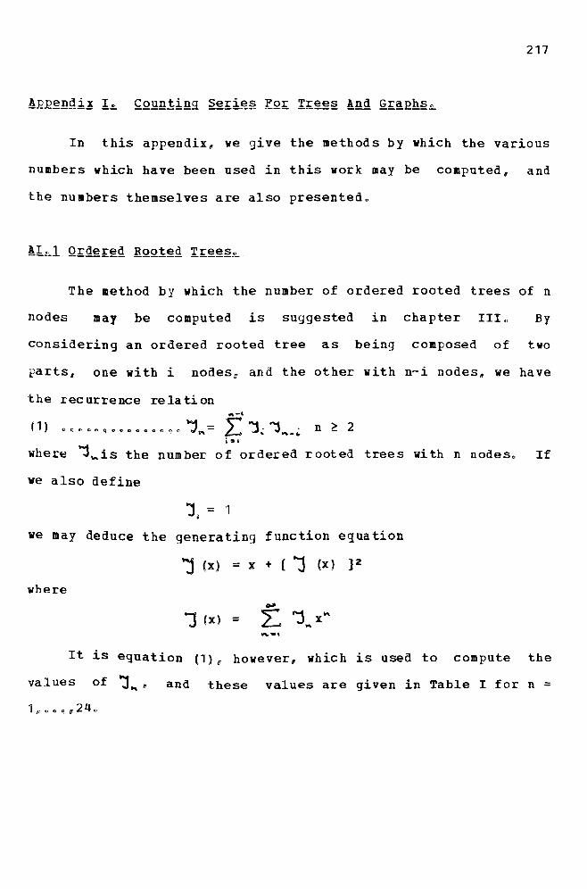
217

In this appendix6 we give the methods by which the variousnumbers which have been used in this work may be computed, andthe numbers themselves are also presented.

The method by which the number of ordered rooted trees of nnodes may be computed is suggested in chapter IlIa Byconsidering an ordered rooted tree as being composed of twoparts, one with i nodes~ and the other with n~i nodes6 we have

the recurrence relation ..-,(1) o 0 n • a q • 00 • o. 0 a 0 ":1....= L J~"3 ..._.: n ~ 2

t ••

where j",is the number of ordered rooted trees with n nodes. Ifwe also define

j = 1j

we may deduce the generating function equation

j (x) == x + {J (x) J2where

1(x) =",-w,

It is equation (1)0 however, which is used to compute thevalues of j ..fI and these values are given in Table I for n =

218

n J..1 12 13 24 55 146 427 1328 4299 1430

10 486211 1679612 5878613 20801214 74290015 267444016 969484517 3535767018 12964479019 47763870020 176726319021 656412042022 2446626702023 9148256364024 343059613650

219

It was demonstrated in chapter III that of the two methodsfox' counting unordered rooted trees discussedc each was(~erivable from the other by a suitable piece of algebra on the';enerating function e,;,uationsr

The Cayley method of counting trees was the simpler toimplement,. but it involved (Jenerating a11 the partitions of n -·1

(tor the number T~ of trees with n nodes)" If it is onlyrequired to find the values of T~ for n = lp26 etcoo a methodusing Harary and Prins equation is more convenient. Harary andPrins shoved that if

0/1

T (x) ::: L T", x'"....:.,

where T~ is the number of trees vith n nodeso thenT (x) = x exp f ~ T (xV') / r}

Now let

A(x) - T(x) / xand

where

QP

B (x) = La T ex"') / r., Cl

A(x) = a.." a,x + a~x2 + o~o

and

then

A (x) = exp I B (x) }Differentiating with respect to x, we have

A~ (x) = exp { B(x) J BQ (x )

::: A (x ) B v ex)

220

This immediately leads toa I + 2a~x + 3a~x 2 + o c < = (a0 + a \x + aa X 2 + o ~ ~ )

or

na~ - a.onb" + a. (n-1)b,,_,+ u,,"

(_2) <:>"OCl()O~C::CO~<!c)C'lOna""

Now we also have

~

~B (x) = T(x"')/r = L ~ A (x'")... -:., 't':. I ..,.

.L eo - ()Q -2: b",x" 2: V' L le:r= x a",x

.. =0 .,:, ..,."'''0and thus

b~ = /_: a~/r,.(It. ....)= ...V~I.Ie.~~

Thus replacing k+1 by Po and multiplying by nu we have(3 ) 2: nat'-,=

.,~,..."'.~~I

.2: pa,,_1ott ~i..,..~~ ...., \0\

Equations (2) and (3)p together with the relation

T ... = a ..._1

are sUfficient to calculate all the also bUs and T's.numbers are given in Table II"

These

221

n T",

1 12 13 24 45 96 207 488 1159 286

10 71911 184212 476613 1248614 3297315 8781116 23538117 63484718 172115919 468867620 1282622821 3522183222 9705518123 26828285524 74372498425 206717464526 575963651027 16083734329

222

A similar technilue may be used to compute the number oftrees with n nodes and height be Riorda n (1960) shows that

.f"...I)(X) c» Tt")(x") /r= x exp { L. 1where T(")(x)

v,.,is the generating function for the numbers of trees

with maximum height h< The generating function for trees withheight exactly h is therefore

.f~(X) _. ~_I'X)

If we now define

and

Bl"'>{x) = t.. .f~)(x"") / r'Y'~I

by analogous manipulation to that used previously v we bave~+I) ~. bU.' (1..1)na.. = L... 1. \ a",,_ ..

~ Co'and

nb(.~)=t\

Now by choosing suitable boundary conditionso namely

for all n z 2and

for all h ~ 1

we may compu te the values of These numbers for n =10ee<620 and h = Onc~ 0019 are given in Table 111<

223

n 1 2 "3 4 5 6 7

h

0 1 0 0 0 0 0 0

1 0 1 1 1 1 1 1

2 0 0 1 2 4 6 10

11 0 0 0 1 3 8 184 0 0 0 0 1 4 135 0 0 0 0 0 1 56 0 0 0 0 0 0 "1

n 8 9 10 11 12 13 14h

0 0 0 0 0 0 0 0

1 1 1 1 1 1 1 12 14 21 29 41 55 76 1003 38 76 147 277 509 924 16484 36 93 22S 528 1198 2666 58155 19 61 180 498 1323 3405 85576 6 26 94 308 941 2744 7722

7 1 7 34 136 487 1615 50798 0 1 8 43 188 728 25939 0 0 1 9 53 251 1043

10 0 0 0 1 10 64 32611 0 0 0 0 1 11 76

12 0 0 0 0 0 1 12

1"3 0 0 0 0 0 0 1

224

n 15 16 17 18 19 20

h

0 0 0 0 0 0 0

1 1 1 1 1 1 12 134 175 230 296 384 489

3 2912 5088 8823 15170 25935 44042

4 12517 26587 55933 116564 241151 495417

5 21103 51248 122898 291579 685562 15992096 21166 56809 149971 390517 1005491 2564164

7 15349 45009 128899 362266 1002681 27404488 8706 27961 86802 262348 776126 22564189 3961 14102 47816 156129 494769 1530583

10 1445 5819 21858 77878 266265 88088311 414 1948 8282 32695 121963 43516812 89 516 2567 11481 47481 18490313 13 103 633 3318 15564 6724914 1 14 118 766 4218 2069715 0 1 15 134 916 528516 0 0 1 16 151 108417 0 0 0 1 17 16918 0 0 0 0 1 18

19 0 0 0 0 0 1

225

Table IV gives the nu.ber of free trees with n nodes for n

1,<~o,27, and these are computed directly fro. the values of

Tn (given in Table II) using otter's formula:t (x) = T (x) -.! { T (x) 2 -- T (X2)

1}

is the genera ting function for

free trees, from which we obtain:!'4Vt" = T.. - 6 L. T.. T~ + t T "/~"~I1. .1

1''"\.....where T..,...is considered to be zero when n is odd,

226

n t~1 12 13 14 25 36 67 118 239 47

10 10611 23512 55113 130114 315915 774116 1932017 4862918 12386719 31795520 82306521 214450522 562375623 1482807424 3929989725 10463689026 27979345027 751065460

227

In Harary ( 1955)nodes and m lines<

we learn how to count the graphs with nThis methodu however, involves the

~eneration of all the cycle classes of permutations in thesymmetric group of order n~ which implies the generation of allthe partitions of n. A program was written to obtain thesevalues, but the method was extremely time consuming, and so novalues were obtained for n > 7. The values which were computedare given in Table v. A slightly quicker method for computingthe total number of graphs of n nodes is based on the method ofDavis (1953)0

228

n 1 2 3 4 5 6

m

0 1 1 1 1 1 1

, , , 1 1 1

2 1 2 2 2

3 1 3 4 5

4 2 6 9

5 1 6 15

6 1 6 21

7 4 24

8 2 249 1 21

10 1 1511 9

12 513 214 1

15 1

229

In chapter IV it vas pointed out that Corneil's alJorith~only works in time proportional to nS provided the ~raph underconsideration does not contain a rarticular type of subgraph.The condition on this sub]raph is that it should not be2--strongly regularo

(VrE) inwhich

(a) for any two nodes x,y E V, Sot~I {vI v € V, (x;v) E E, (y,v) ~ Ell = P~.t{ v [v t V, (x e v ) t: EIr (y, v) f E }I = P':'t{ v I v ~ V" (x,v) + Eo (y c v) f El! == p.!o

(a) f or any two nodes x,y Eo Vg Soto (x , y) t EgI{v Iv £ Vg (xt' v) E: Ell (Yu v) E. E }I = P:-:t{v Iv E. Vo (x c v) ~ E" (Ye v) • Ell = p;:'

I (VI v E: Vo ex II v) t Ee (y Q v) f Ell = P:'where It are constants for a particular graphoP':i

It can be seen that this concept is an extension to twonodes, taking into account the two cases where the nodes are~oined and not joinedg of the concept of regularitYIJ which couldbe restated as

for any node Xc

t{ vt v £-: VC' (x I' v) E: E} I = k

I (vI v " Vu (xu v) f Ell = 1 (= n _. k)

From this definition of 2~'strong regularity ve can see(i) G is regular with degree k

(i i) k = 1 + p!. + P :0

230

(iii) k 0» + 0= P.. PI.• I ,

(Lv) n = 2 + POI + 2PI. + POG

(v) n = 2 + p~ + 2p~0I + p;.

For the graph infig. 10 II we haven = 100 k = 3, 0, , 2P.. = P.• =I 4, u 1}loo = p" =0 2, P:' 31',. = =

This graph, however"also transitive

definition of

is(see

chapter IV for the

transitive) 0

Corneil shows that in a 2-SR graph, each node has the samevertex quotient grapho and gives an example of a 2-SR graphwhich is not transitiveo This graph has 26 nodes8 and is thesmallest known non-transitive 2-strongly regular graphc

In order to distinguish between nodes of a 2-SR graphc the2-vertex quotient graph is definedo A partitioning of the nodesof the graph into the sets {xJu ly)o V-[xoy} for some pair ofnodes x and y, gives a starting partitioning of the nodes forthe refinement algorithmc The final partitioning given by thealgorithm defines a quotient graph which is known as the2-vertex ~uotient graph for the nodes x and y, and this graph iscalled Q_jC Thus for any node Xo we have a set or family of2.-vertex quotient graphs Q-3 for all y E V-{x}c

231

regularity.

The idea of 2-strong regularity may be extended to 3-strong

(a) for all xcY,z £ Vu s,t.

A graph G = (VoE) is 3·'strongly regular if:

I{vlv e VC'(VeX) '" E, (VI'Y) ~ Eo (VI/z) ~ Ell = p:',',J{V1V ~ VI' (VoX) e E, (veY) ~ E, (v,z) ;. EJI = p~:~J{vlv ~ s , (VeX) ~ E, (VeY)

I{vlv ~ V,(vl,x) • E, (VoY)

+- Eo (v,z) 4. E II =;. Eo (v,z) i Ell =

P"',."p!:!o

(a) for all xlly,2 ( V, sc,to, (x,y) e Eo (y,z) tE; El' {zox} <1= E"

J{ V J v E:. V If (v l' x) ~ E" (v, y) t£. Eo (v , z) ~ E J I = P:!~

J[vlv E: Vo (vrx) £. E, (veY) E: EQ (v,z) 4: El! = P~I:

I { v I v e: V, (V o x) £0 E u

(v , z ) E:- E 11 = pliO(OG

"QP'OO

I{vlv Eo Vu (VIOX) t Eo (voY) E;. EQ (voz) ~ Ell = P~I':.

Ifv)v" s , (vex) t E" (v,y) ~ EQ (v,z) <I El! = p~

(a) for all x,y,z ~V, seL, (x,y) ~ s, (y,z) f El' (z,x) +- E/1

J[Vlv ~ Vu (vox) ~ E,

I{Vlv ~ V" (v"x) ~ Eo

(V u y) E- Eo

(voy) ~ Eq

(v, z) 4= E} I

(VeZ) f Ell 100= puo

I{V!v ~ s , (V,x) ~ E .. (V"y) et E. (v,z) ~ Ell = p::~l{Vlv E; Vc (vox) ~ E" (VoY) 4 EQ (v,z) 4. Ell = p:~J[ V) v ~ V/1 (VeX) +- Eo Cv 0 y) fE, (V, z) It E II = P::.'

I{vlV E- Vo (v"x) t E, (V,y) (V,Z) fEll 1.00= poo..:»

(xoY) 4= Eo (y ..z) ¢ E, (z"x) ~ Eo

I{vlv ~ Vu (vlOx) i: E, (v,y) ~ El' (v,z) ~ Ell::;: pi,7'

I{v) V f:; V 0 [v If X) ~ ED

J{VJV f Vu (VeX) ~ E,

I{ v Iv {: V u (V 0 X) 4 Eo

(V, z) f E 11

(V, z) + E 11

(v,z) fEll

(V,y) f Eo

(VeY) f E,

232

The property of h-strong regularity can be definedu but inorder to do so, it is necessary to specify all nono-isomorphicgraphs of order h. An ~-vertex quotient graph is found in theobvious way by distinguishing h vertices at the start of thepartitioning algorithm. A family of h-vertex quotient graphsfor a given node x is the set of all h-vertex quotient graphsfor which x is one of the distinguished nodes.

The determination of h-strongly regular graphs or subgraphsmakes the full graph isomorphism algorithm less efficient. as itincreases the power of n to which the time taken by thealgorithm is proportional.