AN ANALYSIS OF SUBSTITUTION RELATIONSHIPS

BETWEEN SHORT AND LONG STAPLE COTTON

by John Craven

Research Paper for

Agricultural Economics 430

Summer, 1969

TABLE OF CONTENTS

Page I• INTRODUCTION . . . . . . ...... . ..... 1

Problem Statement ..........• . . . . . . . . 1 Objectives ......... . q .............. 3 Review of Literature ........ 5

II. CONCEPTUAL FRAMEWORK . ..................... 7 III. RESEARCH METHODS AND PROCEDURES ............... 16

IV. FINDINGS .......................... • 22 Trends in Supply and Disappearance of U. S. Upland Cotton . 22 Review of Related Work .................... 29 Least Squares Estimates of Short and Long Run Elasticities of Substitution ....................... 32 Simultaneous Equations Method for Estimating Structural Coefficients ................. . . . . . . . 35

V.SUMMARYAND CONCLUSIONS ........... ....... 37

BIBLIOGRAPHY

APPENDIX

'p.

INTRODUCTION

Statement of the Problem

Total disappearance of United States Upland Cotton has been

relatively stable since the early 1930ts. However, within this

aggregate disappearance the importance of short staple cotton' has

declined considerably. A brief review of historical data helps to

point out the degree of this decline. During the 1938-1941 period

disappearance of short staple cotton was 48% of the total disap-

pearance of U. S. Upland Cotton. In the 1962-1966 period this

figure had declined to 22%. The decline in the disappearance of

short staple cotton relative to the disappearance of long staple

cotton2 has been accelerated by the following factors:

1. The prices of short staple cotton relative to the prices

of long staple cotton

2. Changes in technology

3. Consumer income, tastes and preferences.

Relative support prices of short to long staple cotton have

apparently been higher in the past than the demand for short staple

1 Upland Cotton stapling less than 1 inch

2Upland Cotton stapling 1 inch and over

2

cotton would justify. This relationship caused large amounts of

short staple cotton that were produced to remain unsold and thus be

accumulated in Commodity Credit Corporation stocks. This relation-

ship has changed somewhat in recent years with the change in

relative price supports.

Changes in technology have had perhaps the most visible

effect on the disappearance of short staple cotton. Increased

spindle speeds of the more advanced textile machinery requires the

use of stronger fibers in order to keep thread breakage low.

Quality tests show that long staple cotton is usually stronger than

short staple cotton. Another technological factor which has caused

a decrease in the use of short staple cotton is the increased use

of cotton/manmade blends. Most of these blends utilize long

staple cotton.

U. S. consumer income has increased in recent years largely

because of the increasing "white collar" working force. As consumer

income increases, and modes of living change, consumers usually

substitute high quality goods for low quality goods. Cloth made of

short staple cotton is coarser than cloth made of long staple cotton;

thus with the rise in consumer income and changes in the mode of

living in the U. S. population, the demand for goods made with

short staple cotton has declined.

In recent years, farmers on the High Plains of Texas have

produced, on the average, approximately 50% of the total United

States short •staple cotton production. Several characteristics of

short staple cotton give it a comparative advantage over long staple

3

cotton in this area. These advantages include a slightly shorter

growing season and better protection against weather due to a

tighter boll.

In recent years textile manufacturers have indicated that

their use of short staple cotton would decline still further if

they had an adequate supply of long staple cotton, regardless of

the price of short staple cotton. In spite of the contentions

made by the textile industry there is considerable evidence that

the disappearance of short staple cotton is;considerabl7affected

by the price relationship between short and long staple cotton.

This price relationship is largely determined by government price

support policy.3 This implies that the loss of market caused by

the downward shift in the demand for short staple cotton can be

offset by a cange in government price support policy. In any case

those people concerned with the formulation of government programs

should be well aware of the existing conditions, the relationships

involved, and the implications they have in formulating public

policy.

General Objective

The general objective of this project was to determine the

effect of relative prices on the disappearance of short and long

staple cotton.

3See Louis Glass' Ag. Eco. 430 report, An Analysis of Substi-tution Relationships Among Different Staple Lengths of Cotton, Summer, 1968.

M

Specific Objectives

There were several specific objectives of this project.

Objective A was to present a review of trends in the supply

and disappearance of U. S. Upland Cotton.

Objective B was to review related work done previously by

Louis Glass and Bob Baxter.

Objective C was to determine an estimate of the short and

long run elasticities of substitution between short and long staple

cotton, utilizing a least squares estimating equation.

Objective D was (1) to determine unbiased estimates for the

structural coefficients of price and disappearance equations for

short and long staple cotton, and (2) utilize these estimates in

determining the respective short and long run elasticities of

substitution.

Procedure

Most of the data used in this report was transformed U.S.D.A.

data. Most of the calculations involved were made by and contained

in Ag. Eco. 430 reports by Louis Glass and Bob Baxter.

Objective A was achieved by compiling data contained in

U.S.D.A. publications and presenting it in written and graphic form.

Objective B was achieved by summarizing significant findings

of Glass and Baxter in their Ag. Eco. 430 reports.

Objective C was achieved by obtaining estimates of short and

long run elasticities of substitution between short and long staple

cotton, utilizing a linear least squares estimating method.

5

Objective D was achieved by solving a set of price and

disappearance equations simultaneously. Coefficients obtained for

these equations were then used to determine estimates of short and

long run elasticities of substitution.

Review of Literature

There have been many studies concerning demand interrelation-

ships among competing products. Schultz4 developed the theoretical

framework for the "rough test" to distinguish between competing and

5 completing products. Meinken, Rojko, and King utilized price and

consumption ratios to obtain an estimate of the elasticity of sub-

stitution between beef and pork. Waugh6 utilized lagged price and

consumption ratios of cotton and rayon to obtain estimates for

coefficients of long run demand equations. Working devised a method

whereby the slopes or elasticities of short and long run demand curves

could be obtained simultaneously. A later review by Gislason8

4Schultz, Henry. The Theory and Measurement of Demand. Chicago: University of Chicago Press, 1938. pages 570-571.

5K. W. Meinken, A. S. Rojko, and G. A. King. "Measurement of Substitution in Demand from Time Series Data--A Synthesis of Three Approaches". Journal of Farm Economics, Vol. 38 (August, 1956) pages 711-735.

6 Waugh, Frederic V. Demand and Price Analysis - Some Examples From Agriculture. T. B. No 1316, ERS, U.S.D.A. 1964. pages 57-62.

7Working, Elmer J. "Appraising the Demand for Agricultural Output During Rearmament". Journal of Farm Economics. Vol. 34 (May, 1952) pages 206-224.

8Gislason, Conrad. "A Note on Long Run Price Elasticity". Journal of Farm Economics. Vol. 39 (August 1957) pages 798-802.

clarified this method. All of these studies used the single equation

least squares estimating technique. Several authors have suggested

that the assumptions which must hold in order for a single

equation approach to be of value are in fact not always true and

suggest the use of a simultaneous equations approach in these cases.

Haavelmo9 produced the first major article suggesting this approach.

10 lists sts several questions which must be answered before determining

which approach would be more useful. Foote 11 discusses the simul-

taneous equation approach and applies this technique to pork, beef,

and export crops.

Many of the concepts forwarded by these authors will be used

in the preparation of this report.

9Haavelmo, Tryge. "The Statistical Implications of a System of Simultaneous Equations". Econometricia Vol 11. 1943 pages 1-12.

10 Fox, Karl A. The Analysis of Demand for Farm Products. T.B. 1081 U.S.D.A. 1953.

11 J Foote, R. J. Analytical Tools for Studying Demand and Price Structures. Ag. Handbook No. 146 U.S.D.A.

CONCEPTUAL FRAMEWORK

Relative Demand and Related Concepts

Relative demand can be defined as the quantity of one product

(A) that will be consumed relative to the quantity of another product

(B) at all alternative relative price levels of A to B, when all

other factors affecting the demand for either product are held con-

stant. Figure 1 illustrates a relative demand curve for two com-

peting products A and B. It can be seen that when the price ratio

is lowered from point 1 to point 3, the consumption ratio of A to B

increases from point 2 to point 4. Figure 2 illustrates a case in

which the relative demand curve shifts from D1 to D2. This can occur

due to changes in technology, consumer income, tastes, or preferences.

In order for the relative quantity of A consumed to remain at the

same level on curve D2 as on curve D1, the price ratio must decrease

from point 1 to point 3. However, if the price ratio remained at its

previous level, the relative quantity of A consumed would decrease

from point 2 to point 4. This concept implies that in the case of

two competing commodities, a loss in consumption of one commodity

can be offset by lowering the relative price of that commodity.

Therefore, if short and long staple cotton do in fact act as sub-

stitute goods, and the demand for short staple cotton shifts down-

ward over time, relatively more short staple cotton would be con-

sumed if the price ratio of short to long staple cotton were lowered.

8

The degree of substitutability can be measured by the elasticity of

substitution. Accuracy of the estimate for the elasticity of sub-

stitution depends upon the validity of the method used to obtain the

estimate. If the variables used in a least squares analysis do not

meet certain specified conditions, a simultaneous equation approach

is necessary for an unbiased estimate.

"Rough Test"

Schultz 12

proposed the following definition for perfectly

completing and perfectly competing commodities:

Two commodities are perfectly completing if they can-not be used separately but only jointly in a fixed ratio. Two commodities are perfectly competing if they can be substituted for each other in a certain fixed constant ratio.

While he states that these are not precise definitions for

intermediate cases of interrelated products, he proposes that they

be used in formulating a "rough test" to determine whether or not

two commodities are completing or competing in comsumption.

According to the "rough test" two commodities are completing if the

ratio of the two quantities consumed fluctuates relatively less

than their price ratio. The commodities are comDeting if their

price ratio fluctuates relatively less than their consumption ratio.

Therefore, if two commodities are substitute goods (competing), a

12 Schultz, Henry. The Theory and Measurement of Demand. Chicago: University of Chicago Press, 1938. pages 570-571.

10

small change in their price ratio would cause a relatively larger

change in their consumption ratio.

Elasticity of Substitution

Elasticity of substitution is defined as the percentage change

in the consumption ratio of two competing goods associated with a

small percentage change (usually 1%) in the price ratio of these

goods. Expressed in equation form:

(1) E =- •-Pr s iPrQr

where E = the elasticity of substitution

Q-r = the consumption ratio of the two competing goods

Pr = the price ratio of the two competing goods

= a small change

Values of E indicate the ease with which one good will sub-s

stitute for another at a particular point on their relative demand

curve. High values of E indicate the goods are easily substituted

while low values indicate the goods are not easily substituted.

Methods of Estimating Elasticities

The usual method employed for estimating elasticities utilizes

a linear least squares regression analysis with the variables expressed

either in natural units or logarithms. When natural units are used

computations such as those in equation (1) are performed. When

logarithms are used elasticities are obtained directly as coefficients.

Several authors have proposed modifications to this method.

Waugh Method 13

Waugh used an estimating equation of the following form to

estimate the long run elasticity of substitution between cotton and

rayon.

(2) Qt = a1 + biPt + b 2 P + b3P(t 6) + b4P(tg)

where Qt = the current 3 year average consumption ratio of cotton to rayon

Pt = the current 3 year average price ratio of cotton to rayon

= the 3 year average price ratio lagged and ' centered 3, 6, and 9 years, respectively.

Waugh then divided the coefficients obtained in the estimating

equation by 3 to put the data on an annual basis and graphed these

values against time to form a "distributed lag curve." Values for

each year on the distributed lag curve were then added and used as

a cumulative weight. Waugh estimated the long run elasticity of

substitution by multiplying this cumulative weight by the mean value

of the price ratio relative to the consumption ratio. A drawback in

using this method is that unequal weights are arbitrarily assigned to

different years of the analysis depending upon the time lag used.

13 Waugh, Frederic V. Demand and Price Analysis. -- Some Examples from Agriculture. T.B. No. 1316, ERS, U.S.D.A. pages 57-62.

12

Working Method 14

Working utilized a single least squares estimating equation

to obtain slopes of short and long run demand curves. Values obtained

for the slopes can then be used to calculate elasticities. Working

used an equation of the following form.

(3) XI(t) = a + blX2(t) + b2X3(tl)

where X, = price

quantity consumed

X3 = average quantity consumed over a designated number of years

t = current year

t-1 = immediately preceding year

He then defined b1 as the slope of the short run demand curve

and postulated the long run demand equation as:

(4) X4 =a+b3X3

where X4 = the average price averaged over the same period of time as used for X3.

He then demonstrated that b3, which is the slope of the long

run linear demand curve, is equal to b1 + b2 in equation 3. As

pointed out by Gislason this means that the slope of the long run

14 As reviewed by Conrad Gislason, "A Note on Long Run Price Elasticity." Journal of Farm Economics. Vol. 39 (August 1957) pages 798-802.

I

13

demand curve is equal to the slope of the short run demand curve

plus the shift coefficient of the short run demand curve which is

attached to the long run variable. These demand equations can be

expressed in terms of quantities dependant upon price with no

change in the concept involved. When the equations are expressed

in this manner the values obtained for the short and long run slopes

can then be multiplied by price/quantity ratios to obtain the

corresponding short and long run elastiticies of substitution.

Simultaneous Equation Approach for

Estimating Structural Coefficients 15

In their discussion of the simultaneous equation approach

Fox and Foote state that:

A single equation least squares analysis of demand assumes (1) that the demand function is such that one variable can be selected as depend nt upon the others, and that all residual errors or disturbances are con-centrated in the dependant variable; (2) that none of the independnt variables in the demand function are __----in fact influenced by or determined simultaneously t1ie dependAnt variable; (3) that the disturbances in the depandnt variable tend to be normally distributed and not serially correlated.

If these conditions do not hold true for the variables used,

the least squares method may not give unbiased estimates of structural

coefficients. The simultaneous equations method can be used to obtain

unbiased estimates of these coefficients. In most discussions of the

15 Thissection is mainly developed from Foote, R. J., and Fox, Karl A. Analytical Tools for Measuring Demand. Ag Handbook No. 64 U.S.D.A., pages 39-45.

14

simultaneous equations approach several basic terms are used. These

are defined below. 16

Structure - process by which a set of economic variables is believed to be generated.

Endogeneous variables - variables whose values are explained by the structure.

Exogenous variables - variables whose values are explained outside the structure.

Predetermined variables - exogenous and lagged endogenous variables.

Model - Set of structures compatible with the researcher's advance assumptions about the statistical universe from which data is drawn.

Two major problems must be dealt with in formulating a simul-

taneous equations system. These include specifying the economic

model and identifying the structural equations. The economic model

must be specified so that the number of structural equations is

equal to the number of endogenous variables whose values are to be

explained by the system. Also, each equation must be identifiable.

If each equation is "just identified," the system can be solved

quite simply. An equation is just identified when: 17

16 Definitionsare from Foote, R. J. Analytical Tools for Studying Demand and Price Structures. Ag Handbook No. 146. U.S.D.A. page 7.

17 IdentificationRules are from Foote, R. J. Analytical Tools for Studying Demand and Price Structures. Ag Handbook No. 146. U.S.D.A. page 62.

15

(5) K**G*_ 1

where K** = the number of predetermined variables in the system but excluded from the equation.

= the number of endogenous variables included in a particular equation.

If these conditions are met it is then possible to transform

the structural equations into least squares equations, each containing

one endogenous variable. Coefficients obtained by least squares

analysis can then be transformed back into estimates of structural

coefficients by algebraic manipulation. These estimates will not

be biased.

RESEARCH METHODS AND PROCEDURES

All data used in this report were secondary and were obtained

from U.S.D.A. publications on cotton.

Objective A was achieved by (1) compiling supply and

disappearance data for short and long staple cotton, and (2) graphing

this data so that trends could be readily seen.

Objective B was achieved by reviewing related work done

previously by Louis Glass and Bob Baxter. Significant findings of

Glass and Baxter are presented in this report.

Objective C was achieved by utilizing the Working method to

obtain estimates for short and long run elasticities of substitution

between short and long staple cotton. The following least squares

estimating equation was used.

(6) X1 = a + b 1 X 2

+ b 2 X 3

+ b 3 X

4

where X1 = Qr() the current disappearance ratio of

short to long staple cotton.

= Pr the current price ratio of middling

15/16" to middling 1 1/16" Upland Cotton.

= Pr*_1) the average oI X2 for the preceding

5 years, current year not included.

X4 = time, 1943 = 1

17

The period of analysis was from 1943 to 1966. With the

equation set up in this form b1 is defined as the slope 18 of the

short run relative demand curve and b is the shift coefficient for

the short run relative demand curve which is attached to the long

run variable. The slope of the long run demand curve is defined

as b1 + b2.19 Estimates of the short and long run elasticities

of substitution were obtained by multiplying the slopes of the

short and long run relative demand cUrves by the mean relative price

to the mean relative disappearance ratio.

X

(7) E (short run) = b1 _2 xl

X

(8) E5 (long Run) = (b1 + b2) 2

R

where b1 = slope of short run relative demand curve.

b1 + b2 = slope of long run relative demand curve

= mean of X1 as defined previously

= mean of X2 as defined previously

Objective D wasacheieved by solving a set of structural

equations simultaneously. Coefficients obtained for the structural

equations were then utilized in determining short and long run

elasticities of substitution. The following structural equations

18 Slopeswith quantity ratios on the vertical axis

19 See page 12.

18

were used.

.1

(9) Pr =a +b Qr +b Ps +b T + b Sr (t) 1 11 (t) 12 (t) 13 14 (t)

(10) Qr() = a2 + b21Pr() + b22Pr*(tl) + b23T + b24 Sr()

where Pr(s) = current price ratio of short to long staple cotton.

Qr() = current disappearance ratio of short to long staple cotton.

Ps = current price support ratio of middling / 15/16" to middling 1 1/16" cotton.

T = time, 1943 = 1

Sr() = current supply ratio of short to long staple cotton.

Pr* (t-1) = average Pr() for the preceding 5 years-

not including the current year.

The model or set of structural equations satisfies the rules

of specification and identification. The model is specified so that

the number of endogenous variables whose values are to be explained

(namely Pr() and Qr()) is equal to the number of structural

equations. The structural equations are "just identified". As

stated in the conceptual framework an equation is "just identified"

when:

(11) K** = G* - 1

where K*= the number of predetermined variables in the system but excluded from the equation.

G* - the number of endogenous variables included in a particular equation.

The structural equations used in this system are identified

as follows.

Equation 9

K** = Pr*(l) = 1

= Pr() and Qr() = 2

K** = - 1

Equation 10

K** = Ps (t)

= 1

= Pr() and Qr = 2 (t)

= G* - 1

The following method was used to estimate coefficients for

the structural equations.

A. The structural equations were rewritten to place both

endogenous variables on the same side.

(12) Pr() - bllQr() = a1 + bl2Ps(t) + bT + bl4Sr()

(13) _b2lPr() + Qr() = a2 + b22 Pr* ( 1) + b23T + b24Sr()

B. Equation 12 was multiplied by b21 to obtain equation 14.

Equation 13 was multiplied by b11 to obtain equation 15.

20

(14) b2lPr() - bllb2lQr() = b21a1 + b13b21T + bj2b2lPs(t)

+ bl4b2lSr()

(15) _bllb2lPr() + b11Qr b a +b b T + b b Pr* Ct) = 11 12 11 22 11 23 (t-i)

+ bllb24Sr()

C. Equations 12 and 15, and Equations 13 and 14 were then

added to obtain reduced form equations whose coefficients could be

estimated without bias by a least squares analysis.

a2 + b21a1 (b22 + b13b21)T b23

(16) Qr() = 1 - b11b21 + 1 - b11b21 + 1 - b11b21 Pr*

+ + b11b24) Sr() + b12h21

Ps b11b21 1 - b11b21 (t)

(a1 + b11a2) b13 + b11b22 + b12

(17) Pr() = 1 - b11b21 + 1 - b11b21 1 - b11b21 PS(t)

+ b11b23 Pr* (b14 + b11b24)

1-b b (t-i)+ 1-b b

Sr 11 21 11 21

D. The coefficients for the reduced form equations were then

estimated using a least squares regression analysis. This analysis

was run on the IBM 360 computer at Texas Tech Computer Center. As

can be seen in Step C the reduced form coefficients are in terms of

the structural coefficients. When values are obtained for the

reduced form coefficients the structural coefficients can then be

obtained through algebraic manipulation. For example:

(18) b11b23

b11 = 1 - b11b21

b23

1 - b11b21

Estimates of the structural coefficients were then used in

computing the short and long run elasticities of substitution. The

method and procedure used were the same as that used in obtaining

Objective C.

21

FINDINGS

Trends in Supply and Disappearance

Of U. S. Upland Cotton

Total supply of U. S. Upland Cotton has varied considerably

from year to year since 1935 but has trended upward since reaching

a low point in 1947. Total supply of short staple cotton declined

considerably in the 1935-1950 period and has trended slight upward

since 1950. The proportion of the short staple supply composed of

the longer staple lengths in that group (middling 15/16" and

middling 1 1/16")has increased rather steadily since 1937 and corn-

prises a major portion of the total short staple cotton supply.

These relationships can be seen in figure 3.

Trends in the disappearance of U. S. Upland Cotton point out

the declining importance of short staple cotton. Figure 4 indicates

that total disappearance of U. S. Upland Cotton has tended to

increase slightly since 1934. The disappearance of short staple

Cotton has decreased in this period. Figure 5 indicates the

declining importance of short staple cotton in relation to total

U. S. Upland Cotton disappearance. Domestic Mill consumption accounts

for a large proportion of total U. S. Upland Cotton disappearance

(see figure 6). However, since 195220 exports have risen to a level

20 Exportdata on a staple length basis was first made available in 1952.

23

of approximately equal importance as domestic consumption in the

disappearance of short staple cotton (see figure 7). In view of the

trend towards utilizing more long staple cotton due to technological

reasons the export market will probably continue to be of major

significance as far as consumption of short staple cotton is concerned.

25

E±Th f- i1 i

_ _

r_

*:

31-

HE EE:

_ tTL

J:jT - - - - _______ - --. ,

-__:iE:

±:tJ4: _I1

V TEI _

-

26

+: J

-*+ : + LH

E

I 4 Ei 17- E _F:

: ±4ri- j=: TJ4 Ti

1 :

± E1

!: : 1 ... ..

4:

i

L± th:

27

L I t

_

-LI- LH 1:T---

- T - -_I

-!

-± -H- rT:t - - -

!- t 77

ILL

FFf: _ LH4

_

1 ±

EL

4: -

- - _

- - + _ vl-

- :

ii - -- M

28

llEllIIIIOI r MOMMIMMOMIN

mom MOMMEMEMOMME IMEMEMMEMEMMMM won

INNOMME WIN

MOMMOMMOMMEM MEMEMEME nn

__ __ ____

NONE MEMEMESSIMMIMME E—CIM-MIEFSAIII, ME ~Mffiw= ME

ME MFA LWO—M ME

omfm MOM

Mk= NOWEVAIMIN

Mom 92-MLIIMMN RIMMMMMMMMI Millim FREE

-J.

-

ME • =

MEMEMEMEMEMOSE IN 9.0

MEMO MOMEr MEEMEMSOME

MOMEMEM MINME MOMMOMMEMS MOMMIMMES MEMEMOSEMEMOM In MOMMEMEMEMEM Emmo EME MOMMOMIMMEMEMMOMMEM

ME ME ME

MEMEME ME ME MEMINEMEN

qR

29

Review of Related Work

In his Ag. Eco. 430 report Louis Glass utilized least squares

estimating equations in explaining:

1. The market price ratio of short to long staple cotton.

This variable was represented by the market price ratio

of middling 15/16" to middling 1 1/16" Upland Cotton.

2. The market price differential of short and long staple

cotton again represented by middling 15/16" and middling

1 1/16" differentials.

3. The disappearance ratio of short to long staple cotton.

In explaining the market price ratio, best results were

obtained utilizing the price support ratio of middling 15/16" to

middling 1 1/16" Upland Cotton, time, and the supply ratio of short

to long staple cotton as independant variables. "t" values obtained

for the coefficients indicated that the price support coefficient

was significant at the 99% confidence level, and coefficients for

time and the supply ratio were significant at the 95% confidence

level. A R2 value of .89 indicated that these variables explain

89% of the variation in the market price ratio.

The best results in explaining the market price differential

were obtained using basically the same equation as above, with the

price support differential of middling 15/16" and middling 1 1/16"

replacing the price support ratio. In this equation time was

statistically significant at the 99% confidence level, while the

supply ratio and price support differential were significant at the

30

95% confidence level. The R2 value was again .89. The time period

for both studies was from 1943 to 1966.

Results utilizing the consumption ratio of short to long

staple cotton as the dependant variable were generally not as satis-

factory as results using some form of price as the dependant

variable in terms of R2 values obtained. However, many of the

independant variables used were highly significant. In one equation

the disappearance ratio was estimated, using the market price ratio

and time as independant variables. Coefficients of both independant

variables were significant at the 99% confidence level and the R2

value was .74. However, when the market price ratio lagged one year

was added to the equation, the coefficient for the current market

price ratio was not statistically significant. The time period

used for these equations was from 1938 to 1966.

In brief summary, Glass' results indicate that government

price supports are the dominant factor in explaining market price

ratios and price differentials while time and lagged market price

ratios were the major variables explaining disappearance ratios. 430

Bob Baxter's Ag. Eco.'report was concerned mainly with

determining estimates of the short and long run elasticities of

substitution between short and long staple cotton. He estimated

- the:short run elasticity of substitution by utilizing a least

squares estimating equation in which the first difference 21 of the

21 Changefrom the preceding year's value

31

disappearance ratio (ratio of short to long staple disappearance)

was dependant upon the first difference of the price ratio. The

price ratio utilized was the market price of middling 15/16" to

middling 1 1/16" Upland Cotton. The equation utilized logarithms

to put the coefficients on a percentage basis. When using this

procedure the coefficient of the price ratio is an estimate of the

elasticity of substitution. He obtained a value of -6.02 for the

short run elasticity of substitution.

Baxter used a method presented by Waugh for determining the

long run elasticity of substitution. This method is reviewed in

the conceptual framework. He used three basic natural and logrithmic

least squares estimating equations in which (1) a centered 3 year

moving average of the disappearance ratio between short and long

staple cotton and (2) the first difference of this value were used

as dependant variables. Independant variables included were (1) a

centered 3 year moving average of the price ratio of short to long

staple cotton, (2) various lagged values of these price ratios, and

(3) time. His results showed that the moving averages lagged for a

period longer than 3 years were of minor importance. The moving 41

averages which were current or lagged for periods up to 3 years

were of major significance. Time was also of major significance.

He concluded that the elasticity of substitution between short and

long staple cotton is very elastic in the short run, but his findings

were generally inconclusive as far as an estimate for the long run

elasticity of substitution was concerned.

32

Least Squares Estimates for

Short and Long Run Elasticities of Substitution

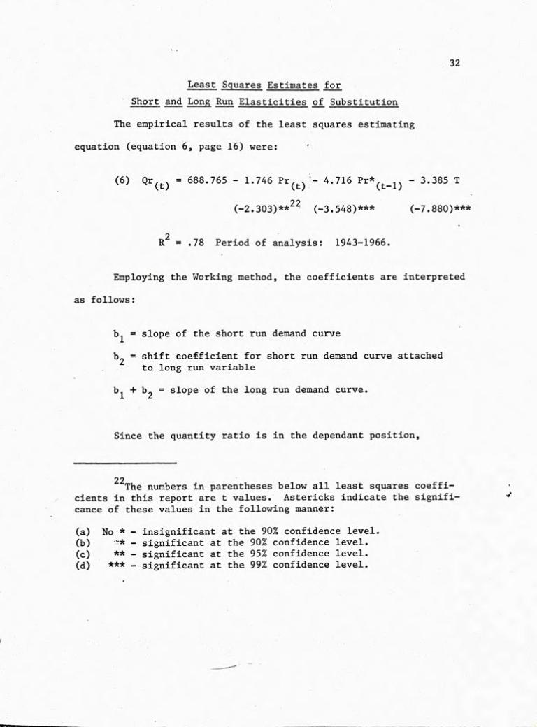
The empirical results of the least squares estimating

equation (equation 6, page 16) were:

(6) Qr() = 688.765 - 1.746 Pr()_ 4.716 Pr*( 1) - 3.385 T

(-2.303) 22 548)*** (-7.880)***

R2 = .78 Period of analysis: 1943-1966.

Employing the Working method, the coefficients are interpreted

as follows:

b1 = slope of the short run demand curve

b2 = shift coefficient for short run demand curve attached to long run variable

+ b2 = slope of the long run demand curve.

Since the quantity ratio is in the dependant position,

22 Thenumbers in parentheses below all least squares coeffi-cients in this report are t values. Astericks indicate the signifi-cance of these values in the following manner:

(a) No * - insignificant at the 90% confidence level. (b) * - significant at the 90% confidence level. (c) ** - significant at the 95% confidence level. (d) *** - significant at the 99% confidence level.

33

X (19) E (short run) = b1 :2

xl

- -1.746 93.129 39.446

= -1.746 2.361

= -4.122

(20) E (shot run) = (b1 + b2) - $ xl

= -6.462 • 2.361

= -15.257

The signs of the coefficients in the estimating equation are

consistant with economic theory. The coefficient of time indicates

a downward trend in the consumption ratio of 3.385 percentage

points per year, with the value of all other independant variables

held consistant. "t" values for the coefficients indicate that all

independant variables used are of major importance in explaining

the disappearance ratio.

Algebraid signs of the elasticities of substitution indicate

that a change in the price ratio will be accompanied by a change in

the opposite direction in the disappearance ratio. As indicated by

the value for the short run elasticity of substitution, this change

will be relatively large in the first year. If the price ratio

changes and is held at its new level for a period of 6 years the

change in the disappearance ratio will be much larger. The value

for the long run elasticity of substitution indicates this relationship

- +- 34

-4----- .'-- -I

I!!! zt4tfl

JE1 4 :

ThH it

ti L

- t

fl

---

-- - L

---- - _ - -- - t

-- -- - { --

KF7-

71

it

---- - r- _ I 1 r -

_ TTT --L

¶+-

_____

- - - - -t

- t

35

Simultaneous Equation Method for

Estimating Structural Coefficients

The empirical results of the reduced form least squares

estimating equations 23 were:

(16) Qr() = 488.128 - 2.344T - 3.125Pr*( 1) - 1.448Ps(t) + .241Sr()

(_4.071)***(_2. 008)* (-1.173) (1.837)*

R2 = .81 Period of analysis: 1943-1966

(17) Pr() = 74.0 - .420T - .449Pr*( 1) + 749Ps - .O76Sr()

(_4.091)***(_1.616) (3.396)*** (_3.242)***

R2 = .91 Period of analysis: 1943-1966

By transforming the coefficients back into the structural

equations 24

(9) Pr() = 2.810 + .144Qr()+ .957Ps(t) - .083T .11lSr()

(10) Qr() = 629.259 - 1.933Pr() - 3.994Pr*( 1) - 3.156T + .087Sr()

By utilizing equation 10 in the Working method for obtaining

elasticities, we obtain:

23 Equations 16 and 17, page 20.

24 Equations9 and 10, page 18.

W.

(21) E S (short run) = b

Pr () 1

Qr()

- 93.129 -1.933 39.446

= -1.933 2.361

= -4.564

(22) E (long run) = (b1 + b2) Pr ()

S

Qr (t)

= (-1,933 - 93:129 39.446

= -5.927 2.361

= -13.994

In reduced foirn equation (16), all signs of coefficients are

consistant with economic theory. The coefficients are significant

at the 90% confidence levelwith the exception of the coefficient

far the price support ratio. In equation (17) the sign of the 5 year

average price ratio lagged one year is not consistant with economic

theory. However its coefficient is not significant at the 90% confi-

dence level. All other signs of the coefficients are as expected

and are highly significant. The coefficient of time was highly sig-

nificant in both reduced form equations.

When the reduced form coefficients are transformed into

structural coefficients, all signs are as expected. The coefficients

of equation 10, which were used in calculating elasticities, are

quite similar to those obtained in least squares equation (6).

Elasticities calculated by utilizing equation 10 have the expected

signs and are comparable to those obtained in the single equation

least squares analysis.

37

SUMMARY AND CONCLUSIONS

The trends in the supply and disappearance of short staple

cotton strengthen the hypothesis that the demand for short staple

cotton is shifting downward over time. Least squares regression

analysis which include time as an independant variable affecting

consumption lend further support to this hypothesis.

This study provides strong evidence that lower relative

prices for short staple cotton would cause its consumption to

increase in spite of the trends towards utilizing more long staple

Cotton.

According to theory and the values obtained for short and

long run elasticities of substitution a 1% change in the relative

price of short staple cotton would cause its disappearance ratio

to change almost 4% immediately. The change in the disappearance

ratio would be in the opposite direction from the change in the

price ratio. If the price ratio was held constant for 6 years •1

after changing the disappearance ratio would change approximately

13-15% within the 6 year period.

No definite conclusion can be drawn concerning which method

(least squares or simultaneous equations) is "best" in determining

the elasticities of substitution. Both methods yield comparable

values and the elasticity of substitution concept is best used

in determining the relative degree of change, not as a measure of

the exact magnitude of change.

BIBLIOGRAPHY

Foote, R. J. Analytical Tools for Studying Demand and Price Structures. Agriculture Handbook No. 146. U.S.D.A.

Foote, R. J.; and Fox, Karl A. Analytical Tools for Measuring Demand. Agriculture Handbook No. 64. U.S.D.A.

Fox, Karl A. The Analysis of Demand for Farm Products. Technical Bulletin No. 1081. U.S.D.A., 1953.

Fowler, Mark L. An Economic-Statistical Analysis of the Foreign Demand for American Cotton. PhD. Dissertation, University of California at Berkeley.

Gislason, Conrad. "A Note on Long Run Price Elasticity". Journal of Farm Economics. Vol. 39 (August 1957) pp 798-802.

Haavelmo, Trygve. "The Statistical Implications of a System of Simultaneous Equations". Econometricia. Vol. 11, pp. 1-12.

Lerner, Elliot B. An Econometric Analysis of the Demand for Pecans with Special Reference to the Demand Interrelationships Among Domestic Tree Nuts. Masters Thesis, Oklahoma State University, 1959.

K. W. Meinken, A. S. Rojko, and G. A. King. "Measurement of Substi-tution in Demand from Time Series Data -- A Synthesis of Three Approaches". Journal of Farm Economics. Vol. 38 (August 1956) pp. 711-735.

Schultz, Henry. The Theory and Measurement of Demand. Chicago: University of Chicago Press, 1938.

Waugh, Frederic V. Demand and Price Analysis -- Some Examples from Agriculture. Technical Bulletin No. 1316, ERS, U.S.D.A., 1964.

Working, Elmer J. "Appraising the Demand for Agricultural Output During Rearmament". Journal of Farm Economics. Vol. 34 (May 1952) pp. 206-224.

Table 1. Supply and Disappearance of U. S. Upland Cotton: By Staple Lengths, 1928-1966.

Disappearance Supply

15/16" Domestic 15/16" and All Mill Con- and All

Year 31/32" < 1" Staples suraption 31/32" < 1" Staples

1000 running bales - 1000 running bales 1928 3,255 11,009 14,565 7,091 3,652 12,212 16,688

1929 2,320 9,689 12,238 6,106 3,145 12,408 16,642

1930 2,718 8,691 11,800 5,263 4,246 13,297 18,046

1931 3,334 10,337 13,301 4,866 6,038 16,730 22,861

1932 4,176 10,795 14,191 6,137 6,375 15,687 22,261

1933 4,078 9,047 13,086 5,700 6,191 13,927 20,724

1934 2,239 6,117 9,967 5,360 4,178 11,219 17,096

1935 3,168 8,176 12,202 6,351 4,427 12,285 17,532

1936 3,017 7,956 13,072 7,950 3,876 11,021 17,454

1937 3,083 7,291 11,183 5,748 5,897 15,173 22,619

1938 2,869 5,724 10,091 6,858 5,938 13,522 23,034

1939 3,266 7,411 13,942 7,793 5,849 13,602 24,395

1940 2,328 4,303 10,703 9,721 5,582 11,115 22,714

1941 3,184 4,780 11,970 11,170 5,519 10,741 22,445

1942 2,881 4,921 12,308 11,100 4,921 10,747 22,838

1943 2,465 4,474 11,040 9,943 4,633 10,534 21,599

1944 2,386 4,259 11,384 9,568 4,396 10,128 22,390

1945 2,479 5,515 12,650 9,163 3,707 8,477 19,815

1946 1,993 4,326 13,288 10,024 2,336 4,858 15,680

1947 1,719 3,689 10,960 9,354 2,117 4,382 13,948

1948 1,705 3,654 12,349 7,795 2,061 4,155 17,565

1949 2,028 4,715 14,376 8,850 2,732 5,985 21,121

1950 1,605 3,302 14,477 10,509 1,796 3,612 16,591

1951 1,432 3,394 14,461 9,196 1,816 4,303 17,170

1952 1,417 3,256 12,089 9,461 2,098 5,011 17,567

1953 1,477 2,817 12,181 8,576 2,853 5,706 21,731

1954 1,551 3,105 12,128 8,841 3,294 6,827 23,127

1955 1,258 2,641 11,118 9,209 3,304 7,338 25,500

1956 1,623 3,715 16,233 8,608 3,626 7,488 27,484

1957 1,712 2,820 13,459 7,999 3,869 6,532 22,052

1958 2,442 2,974 11,228 8,703 4,622 6,695 19,946

1959 3,538 5,737 15,774 9,017 4,777 7,169 23,164

1960 3,718 4,205 14,512 8,279 4,270 4,804 21,589

1961 2,637 3,076 13,615 8,953 3,814 4,454 21,341

1962 2,019 2,365 11,474 8,419 4,237 5,219 22,479

1963 2,382 3,041 14,023 8,609 4,656 6,729 26,134

1964 1,494 2,785 13,123 9,171 4,467 7,126 27,142

1965 2,087 2,407 12,300 9,496 5,920 8,337 28,866

- 1966 1,913 3,567 13,886 9,485 5,647 8,489 26,056

(e 1)

Sources of Data for Table 1: Disappearance and Supply:

1928-1934 - Statistics on Cotton and Related Data, 1920-1956. Statistical Bulletin No. 99 (Revision of February 1957) Agricultural Marketing Service. U.S.D.A. Table 98, page 120.

1935-1966 - figures are from Statistics on Cotton and Related Data, 1930-1967. Statistical Bulletin No. 417. Economic Research Service. U.S.D.A. Table 108, pp. 139-140.

Domestic Mill Consumption: 1928&1929 - Statistics on Cotton and Related Data, 1925-1962.

Statistical Bulletin No. 329, ERS, U.S.D.A. Table 1, page 1.

1930-1966 - figures are from Statistics on Cotton and Related Data, 1930-1967. Statistical Bulletin No. 417. Economic Research Service. U.S.D.A. Table 9, page 8.

Table 2. Average Market and Government Support Prices Of U. S. Upland Cotton: Specified Staple Lengths,

1943-1966.

Middling 15/16" Middling 1 1/16"

Avg. Mkt. Support Avg. Mkt. Support Year Price Price Price Price

1943 20.65 19.26 21.82 20.46 1944 21.86 21.08 23.04 22.13 1945 25.96 21.09 26.96 22.29 1946 34.82 24.38 35.45 25.43 1947 34.58 27.94 36.31 28.64 1948 32.15 30.74 33.27 32.34 1949 31.83 29.43 33.22 30.58 1950 42.58 29.45 43.78 30.80 1951 39.42 31.71 40.49 32.96 1952 34.92 31.96 36.00 32.96 1953 33.55 32.70 35.08 34.15 1954 33.88 33.23 36.17 34.83 1955 34.38 33.50, 36.72 35.50 1956 32.35 31.59 35.02 33.99 1957 32.93 31.16 36.12 33.76 1958 32.96 33.63 36.14 36.83 1959 30.27 29.74 33.46 32.84 1960 29.43 27.61 32.43 30.81 1961 32.43 31.49 35.08 34.39 1962 32.26 34.22 34.93 33.77 1963 31.85 31.22 34.68 33.82 1964 22.891 28.70 25.90 31.40 1965 22.441 27.65 25.711 30.55 1966 20.20 19.60 24.73 22.80

11964 and 1965 market prices are adjusted -6.5 and -5.75 cents per pound respectively. Authority: 1964 - Cotton Price Statistics Vol. 46 No. 12, U.S.D.A.

Table 15, page 22. 1965 - Cotton Price Statistics Vol. 47 No. 13 U.S.D.A.

Table 35, page 35. Sources of Data: Columns 2 and 4:

1943-1948 - Statistics on Cotton and Related Data, 1920-1956. Statistical Bulletin No. 99, Agricultural Marketing Service, U.S.D.A. page 158.

1949-1958 - Statistics on Cotton and Related Data, 1925-1962. Statistical Bulletin No. 417, Economic Research Service, U.S.D.A. page 131.

1959-1966 - Cotton Price Statistics. Vol. 48 No. 13, U.S.D.A. page 5.

Columns 3 and 5: 1943-1953 - Cotton Quality. Agricultural Marketing Service U.S.D.A.

1944-1954. 1954-1966 - Cotton Price Statistics, May 1955-1967, U.S.D.A.

Table 3. Price, Consumption and Supply Ratios of < 1" to , 1" U. S. Upland Cotton: 1943-1966

2 Price Market Support

1 Supply Consumption Year Price Ratio Ratio Pr*(l) Ratio Ratio

1943 94.64 94.31 95.45 95.20 68.14 1944 94.88 95.26 95.55 82.60 59.78 1945 96.29 94.62 95.23 74.77 77.30 1946 98.22 95.87 95.29 44.89 48.27 1947 95.24 97.56 95.73 45.81 50.74 1948 96.63 95.05 95.85 30.98 42.02 1949 95.82 96.24 96.25 39.54 48.80 1950 97.26 95.62 96.44 27.83 29.63 1951 97.36 96.21 96.63 33.44 30.67 1952 95.89 96.97 96.46 39.91 36.86 1953 95.64 95.75 96.59 35.61 30.08 1954 93.67 95.41 96.39 41.88 34.41 1955 93.63 94.37 95.96 40.40 31.15 1956 92.38 92.94 95.24 32.45 29.68 1957 91.17 92.30 94.24 42.09 26.51 1958 91.20 91.31 93.30 50.54 36.03 1959 90.44 90.56 92.41 44.81 57.16 1960 90.75 89.61 91.76 28.62 40.80 1961 92.45 91.57 91.19 26.37 29.18 1962 92.36 92.45 91.20 30.24 25.95 1963 91.84 92.31 91.44 34.68 27.70 1964 88.38 91.40 91.57 35.60 26.95 1965 87.28 90.51 91.16 40.62 24.32 1966 81.68 85.96 90.46 48.32 34.57

year average Market Price Ratio immediately preceding but not including the current year

2These ratios are prices of middling 15/16t relative to middling 1 1/16"

Sources of Data: Columns 1, 2, and 3: See Table 2 Columns 4 and 5: See Table 1

Table 4. Disappearance of Cotton Stapling less than 1": 1952-1966

Exports Domestic Consump- Total Year (1000 bales) tion (1000 bales) (1000 bales)

1952 819 2,437 3,256 1953 906 1,911 2,817 1954 845 2,260 3,105 1955 1,116 1,525 2,641 1956 1,743 1,972 3,715 1957 1,587 1,233 2,820 1958 1,314 1,650 2,974 1959 2,393 3,334 5,737 1960 1,966 2,239 4,205 1961 1,543 1,533 3,076 1962 1,155 1,210 2,365 1963 1,524 1,517 3,041 1964 1,244 1,541 2,785 1965 1,146 1,261 2,407 1966 1,618 1,949 3,567

Sources: Exports:

1952 - Cotton Situation. Economic Research Service, U.S.D.A., September, 1953.

1953 - . October, 1954. 1954-1966 - . November, 1955-1966.

Total: See Table 1.

Domestic Consumption: Computed by subtracting Exports from the Total Disappearance.