Embed Size (px)
Citation preview
AN ANALYSIS OF PURE ROBOTIC CYCLES
a thesis
submitted to the department of industrial engineering
and the institute of engineering and science
of bilkent university
in partial fulfillment of the requirements
for the degree of
master of science
By
Serdar Yıldız
July, 2008

I certify that I have read this thesis and that in my opinion it is fully adequate,
in scope and in quality, as a thesis for the degree of Master of Science.
Prof. Dr. M. Selim Akturk (Advisor)
I certify that I have read this thesis and that in my opinion it is fully adequate,
in scope and in quality, as a thesis for the degree of Master of Science.
Assoc. Prof. Dr. Oya Ekin Karasan
I certify that I have read this thesis and that in my opinion it is fully adequate,
in scope and in quality, as a thesis for the degree of Master of Science.
Asst. Prof. Dr. Hakan Gultekin
Approved for the Institute of Engineering and Science:
Prof. Dr. Mehmet B. BarayDirector of the Institute
ii
ABSTRACT
AN ANALYSIS OF PURE ROBOTIC CYCLES
Serdar Yıldız
M.S. in Industrial Engineering
Supervisor: Prof. Dr. M. Selim Akturk
July, 2008
This thesis is focused on scheduling problems in robotic cells consisting of a
number of CNC machines producing identical parts. We consider two different
cell layouts which are in-line robotic cells and robot centered cells. The problem
is to find the robot move sequence and processing times on machines minimizing
the total manufacturing cost and cycle time simultaneously. The automation in
manufacturing industry increased the flexibility, however it is not widely studied
in the literature. The flexibility of machines enables us to process all the required
operations for a part on the same machine. Furthermore, the processing times on
CNC machines can be increased or decreased by changing the feed rate and cut-
ting speed. Hence, we assume that a part is processed on one of the machines and
the processing times are assumed to be controllable. The flexibility of machines
results in a new class of cycles named pure cycles. We determined efficient pure
cycles and corresponding processing times dominating the rest of pure cycles in
the specified cycle time regions. In addition, for in-line robotic cells, the optimum
number of machines is determined for given parameters.
Keywords: In-line robotic cell, CNC, scheduling, bicriteria optimization, control-
lable processing times, robot centered cell, cycle time minimization, manufactur-
ing cost minimization.
iii

OZET
TEK ATAMALI ROBOTIK DONGULER UZERINE BIRANALIZ
Serdar Yıldız
Endustri Muhendisligi, Yuksek Lisans
Tez Yoneticisi: Prof. Dr. M. Selim Akturk
Temmuz, 2008
Bu tezin konusu, aynı tur parcalar ureten, belirli bir sayıda CNC makinadan
olusan robotik hucrelerde ortaya cıkan cizelgeleme problemleridir. Bu calısmada,
dogrusal robotik hucreler ve robot merkezli robotik hucreler goz onunde bulun-
durulmustur. Bu problemdeki amacımız, birim basına dusen uretim maliyetini
ve dongu suresini aynı anda enkuculten robot hareket dongusunu ve bu donguye
karsılık gelen, makinalar uzerindeki uretim zamanlarını bulmaktır. Uretim
endustrisindeki otomasyonlar hucrelerin esnekligini arttırdı. Ancak, robotik
hucrelerde esneklik uzerine literaturde yeterince arastırma bulunmamaktadır. Bir
urun icin gereken uretim islemlerinin tumu bir CNC makinada gerceklestirilebilir.
Ayrıca, CNC makinalardaki uretim sureleri, besleme ve isleme hızına baglı olarak
azaltılıp arttırılabilir. Bu nedenle, bir parca uzerindeki uretim islemlerinin
tek bir makinada yapıldgını ve uretim surelerinin kontrol edilebilir oldugunu
varsaydık. Esnek makinalar, yeni bir dongu sınıfı olan tek atamalı dongulerin
olusturulmasına olanak vermistir. Bu tezde tek atamalı donguler goz onunde
bulundurulmustur. Belirtilen dongu zamanı alanlarında, diger butun tek ata-
malı donguleri basatlayan tek atamalı donguler ve uretim zamanlarını belirledik.
Ayrıca, dogrusal robotik hucreler icin, verilen degerlere gore en iyi makina sayısını
belirledik.
Anahtar sozcukler : Dogrusal robotik hucre, CNC, robotik hucre cizelgelemesi, iki
kriterli eniyileme, kontrol edilebilir uretim zamanları, dongu zamanı enkucultme,
uretim maliyeti enkucultme.
iv
Acknowledgement
I would like to express my gratitude to my supervisors Prof. Dr. M. Selim
Akturk and Assoc. Prof. Dr. Oya Ekin Karasan for their instructive comments,
guidance and encouragement in the supervision of the thesis.
I am also grateful to Assist. Prof. Hakan Gultekin for excepting to read and
review this thesis and for his invaluable suggestions.
Finally, I would like to express my special thanks and gratitude to TUBITAK
for the scholarship provided throughout the thesis study.
v

Contents
1 Introduction 1
1.1 Motivation . . . . . . . . . . . . . . . . . . . . . . . . . . . . . . . 4
1.2 Organization of the Thesis . . . . . . . . . . . . . . . . . . . . . . 4
2 Literature Review 6
2.1 Robotic Cell Scheduling . . . . . . . . . . . . . . . . . . . . . . . 9
2.1.1 Cyclic Scheduling . . . . . . . . . . . . . . . . . . . . . . . 9
2.1.2 Multiple Part-Types . . . . . . . . . . . . . . . . . . . . . 10
2.2 Bicriteria Optimization . . . . . . . . . . . . . . . . . . . . . . . . 12
2.3 Controllable Processing Times . . . . . . . . . . . . . . . . . . . . 13
2.4 Summary . . . . . . . . . . . . . . . . . . . . . . . . . . . . . . . 15
3 Assumptions and Definitions 16
3.1 Bicriteria Solution Procedure . . . . . . . . . . . . . . . . . . . . 19
4 Bicriteria Scheduling in In-Line Robotic Cells 22
vi

CONTENTS vii
4.1 Bicriteria Analysis of Cm1 and Cm
2 . . . . . . . . . . . . . . . . . . 22
4.1.1 Problem Definition . . . . . . . . . . . . . . . . . . . . . . 23
4.1.2 Solution Procedure . . . . . . . . . . . . . . . . . . . . . . 24
4.1.3 Discussion . . . . . . . . . . . . . . . . . . . . . . . . . . . 45
4.2 Optimum Number of Machines . . . . . . . . . . . . . . . . . . . 45
4.2.1 Problem Definition and Solution Procedure . . . . . . . . . 45
4.2.2 Discussion . . . . . . . . . . . . . . . . . . . . . . . . . . . 49
5 Pure Cycles in Robot Centered Cells 50
5.1 Minimizing Cycle Time with Fixed
Processing Times . . . . . . . . . . . . . . . . . . . . . . . . . . . 51
5.1.1 Problem Definition . . . . . . . . . . . . . . . . . . . . . . 52
5.1.2 Solution Procedure . . . . . . . . . . . . . . . . . . . . . . 53
5.1.3 3-Machine Analysis . . . . . . . . . . . . . . . . . . . . . . 64
5.1.4 Discussion . . . . . . . . . . . . . . . . . . . . . . . . . . . 67
5.2 Bicriteria Analysis of Cm2 and Cm
3 . . . . . . . . . . . . . . . . . . 68
5.2.1 Problem Definition . . . . . . . . . . . . . . . . . . . . . . 68
5.2.2 Solution Procedure . . . . . . . . . . . . . . . . . . . . . . 69
5.2.3 3-Machine Case with Controllable Processing Times . . . . 75
5.2.4 Discussion . . . . . . . . . . . . . . . . . . . . . . . . . . . 80
6 Conclusions and Future Work 81
List of Figures
4.1 m-Machine In-Line Robotic Cell . . . . . . . . . . . . . . . . . . 24
4.2 C41 and C4
2 pure cycles . . . . . . . . . . . . . . . . . . . . . . . . 44
5.1 3-Machine Robot Centered Cell . . . . . . . . . . . . . . . . . . . 52
5.2 Cycle time-Processing time region where Cm2 dominates the rest of
pure cycles . . . . . . . . . . . . . . . . . . . . . . . . . . . . . . 62
5.3 3-machine cell analysis . . . . . . . . . . . . . . . . . . . . . . . . 65
5.4 3-machine cell with controllable processing times analysis . . . . . 78
viii

List of Tables
5.1 Some of the robot move sequences and corresponding cycle times
in 3-machine robotic cells . . . . . . . . . . . . . . . . . . . . . . 67
5.2 The feasible pure cycles in the cycle time region K < 12ε + 12δ
and corresponding robot move sequences . . . . . . . . . . . . . . 76
5.3 The processing times of optimum solutions of feasible pure cycles
in the cycle time region K < 12ε + 12δ . . . . . . . . . . . . . . . 77
ix

Chapter 1
Introduction
The automation in manufacturing processes increased as the technology created
special appliances for automation and improved the machines used in today’s in-
dustry. Robots and Computer Numerically Controlled (CNC) machines are the
important automation appliances that are considered in this thesis. Since robots
increase the efficiency and reduce the labor cost, they are used in many diverse
industries such as semiconductor manufacturing industry and electroplating ap-
plications, chemical operations, and metal cutting industry [9]. In this thesis, we
focus on the metal cutting applications in which the machines are predominantly
CNC machines. The robots have different duties in different industries. One of
the most important applications of robots is using them as material handling
instruments. The robot handling costs may constitute from 10% to 80% of total
costs according to the type of manufacturing facility [33]. A robotic cell is de-
fined as a manufacturing cell composed of a number of machines and a material
handling robot. We assume that there are no buffers at or between the machines,
thus, at any time, a part is either on one of the machines, at the input or output
buffers or on the robot.
In this thesis, we focused on the robot move sequence, the processing times
on machines and the design of the robotic cell which are important decisions that
have to be made in robotic cells. For the design of the cell, we consider two differ-
ent layouts. The first cell layout considered is an m-machine in-line robotic cell
1

CHAPTER 1. INTRODUCTION 2
and the second cell layout is an m-machine robot centered cell. There is a single
robot with a single gripper in both of these layouts. For the first cell layout, there
is a bicriteria optimization problem of minimizing the cycle time and minimizing
the manufacturing cost simultaneously. Additionally, as a design problem, the
optimum number of machines in the cell is calculated. For the robot centered
cell, the first problem considered is the minimization of cycle time that results
in the maximization of throughput which is prominent in production planning.
The second problem considered is the bicriteria optimization of minimizing cycle
time and total manufacturing cost simultaneously.
Highly flexible CNC machines are used for metal cutting operations in robotic
cells. The machines and the robot are used simultaneously in robotic cells. The
cutting speed and the feed rate are controllable variables in CNC machines so
that the processing times on these machines can be decreased at the expense of
decreasing tool life and consequently increasing tooling cost. Considering fixed
processing times is not convenient for real life problems in these robotic cells.
For the bicriteria optimization problems considered in this thesis, the processing
times on machines are assumed to be decision variables due to the controllability
assumption.
As the flexibility of machines increase with the technological advance, new
problems arise to be solved. The cyclic scheduling is widely studied in the lit-
erature and we focus on cyclic schedules. In this thesis, we restrict ourselves to
pure cycles resulting from the flexibility of machines. Pure cycles are defined by
Gultekin et al. [12] as the robot move cycles in which the robot loads and unloads
all m machines with a different part during one repetition of the cycle, thus for
each repetition a pure cycle produces m parts. Each part is completely performed
by only one machine and no part is transferred from one machine to another one.
Furthermore, since pure cycles are practical, easy to understand and easy to put
in practice, they could have significant implementation possibilities in industry.
Gultekin et al. [12] considered the case where the processing times of all machines
are fixed and are the same. In this regard, they proved that the set of pure cy-
cles dominate all flowshop type robot move cycles in terms of cycle time. Then,
they showed that two specific pure cycles perform significantly better than the
CHAPTER 1. INTRODUCTION 3
other robot move cycles among the class of feasible robot move cycles and they
derived the regions of optimality for these two cycles. For the remaining region,
they derived the worst case performances of these cycles. However, the bicriteria
problem of finding the best pure cycle and processing times minimizing the cycle
time and the manufacturing cost simultaneously in an m-machine robotic cell is
not studied in the current literature. Hence, we set out to close this gap in the
literature with this study.
For the bicriteria problems considered in this study, the processing times are
decision variables which are determined according to two objectives and these
objectives are minimization of cycle time and minimization of total manufactur-
ing cost. In order to increase the throughput rate, the minimization of cycle time
is more important and it is studied in the literature widely. Although the min-
imization of total manufacturing cost objective is one of the most fundamental
objectives in the manufacturing literature, as far as authors know, in robotic cell
literature, the only study considering this objective is by Gultekin et al. [13].
Since, the problem we are focusing is a bicriteria optimization problem, the effi-
cient solution set is composed of nondominated solutions.
The bicriteria problem that we consider in this thesis is composed of two im-
portant objectives that are thoroughly investigated in the literature separately.
These two objectives are minimizing cycle time and minimizing manufacturing
cost. The complexity of the problems increases when the objective of the prob-
lem is changed from a single objective problem to a multicriteria problem. There
are efficient ways of solving the bicriteria problems in the literature and some of
these solution methods are summarized by Hoogeven [20]. In addition, most of
the real life problems consist of more than one objective. The reason for that is
single objective optimization results in loose solutions for the other performance
measures when there is a trade-off between the performance measures. The single
objective of cycle time minimization may result in a solution that performs ineffi-
cient in terms of manufacturing cost. Since these two objectives are as important
as each other, the solution of bicriteria optimization problem results in solutions
with cycle times and total manufacturing costs which are between the solutions
of minimizing cycle time problem and minimizing manufacturing cost problem,
CHAPTER 1. INTRODUCTION 4
separately. Thus, the focus of this thesis is on bicriteria objective of minimizing
both the cycle time and the total manufacturing cost, simultaneously.
1.1 Motivation
Different from the current literature, for the bicriteria problems considered in
this thesis, our problem is to determine the pure cycles and the corresponding
nondominated processing time vectors in order to minimize total manufacturing
cost and cycle time simultaneously in robotic cells. The considered objectives
are prominent objectives in the literature and this problem is not studied in
the literature. Most of the studies focus on one machine problems since they
are easier to analyze. The complexity of problems increases as the number of
machines in the cell increases. Although they are more complex, we focused on
m-machine robotic cells where m is any positive integer value. In addition, the
most popular cost function used in the literature is a linear cost function however
in reality, the cost functions are mostly not in linear structure. Thus, the cost
function considered in this thesis is a nonlinear, strictly convex and differentiable
cost function. Furthermore, we solve the bicriteria problem for two different cell
layouts which are an m-machine in-line robotic cell and an m-machine robot
centered cell.
1.2 Organization of the Thesis
This thesis is organized as follows: Chapter 2 summarizes the studies in the liter-
ature on robotic cell scheduling, bicriteria scheduling and controllable processing
times. In Chapter 3, the assumptions and definitions used throughout the thesis
are explicitly presented. In Chapter 4, two problems considered in robotic cell
scheduling literature are analyzed for m-machine in-line robotic cells. The first
problem considered is the bicriteria analysis of pure cycles in m-machine in-line
robotic cells. The second problem considered is finding the optimum number of

CHAPTER 1. INTRODUCTION 5
machines in the cell as a design problem. In Chapter 5, there are two problems
to be solved for m-machine robot centered cells. The layout of the cell is changed
to robot centered cell. For an m-machine robot centered cell, the efficient pure
cycles are investigated according to the objective of minimizing cycle time. In
the second problem, controllable processing times are considered and the problem
is investigating the efficient pure cycles minimizing both the cycle time and the
total manufacturing cost simultaneously. Finally, in Chapter 6, the summary of
the thesis and some future research directions are presented.

Chapter 2
Literature Review
In this thesis, we consider a bicriteria optimization problem in robotic cells where
the production process is considered as cyclic. Gultekin et al. [12] and Gultekin
et al. [14] studied on minimizing cycle time in robotic cells. Gultekin et al.
[14] focused on process and operational flexibility and proposed a new class of
robot move cycles named as pure cycles. They proved that this new class of
cycle dominates all classical robot move cycles considered in the literature for
m = 2. Furthermore, they proved that changing the layout from an in-line
robotic cell to a robot-centered cell reduces the cycle time of the proposed cycle
even further, whereas the cycle times of all other cycles remain the same. For the
m-machine case, they found the regions where the proposed cycle dominates the
classical robot move cycles. In addition, Gultekin et al. [12] proved that pure
cycles dominate the flowshop type robot move cycles studied in the literature
according to the single objective of minimizing cycle time. Therefore, we focus
on pure cycles in this study. Furthermore, the new production environments
give us the opportunity to decrease or increase the processing times of jobs in
specified boundaries. The processing speed of machines can be altered to change
the total cost of production as well as the processing times. Using this property,
more economical ways of production can be determined which also maximizes the
throughput rate. So, the processing times are assumed to be controllable in our
study.
6

CHAPTER 2. LITERATURE REVIEW 7
There are many studies on minimizing cycle time in robotic cell scheduling
literature. The minimization of cost objective is one of the prominent objectives in
manufacturing systems, however this objective is not well studied in the literature
on robotic cell scheduling. So, our study is distinctive from the studies considering
only minimization of cycle time or only minimization of total manufacturing cost
in robotic cells. The robotic cell scheduling problems are classified according to
machine environment, processing characteristics and objectives in Dawande et al.
[9] which are described in the following three parts.
1. Machine environment
The robotic cells including single machines for each stage are named as simple
robotic cells or robotic flowshops. If there are more than one machine at least in
one stage, the cell is named as robotic cell with parallel machines. In order to
increase the throughput rate, more than one robot can be placed in the cell. The
robotic cells including one robot is called single robot cells and the cells containing
more than one robot is named as multiple robot cells. The robots studied in the
literature are single gripper robots and dual gripper robots. The single gripper
robots can hold only one part at a time. The dual gripper robots are able to hold
two parts at the same time. The robotic cell considered in this thesis includes a
single robot with a single gripper.
2. Processing characteristics
Most of the studies in robotic cells assume that there is no buffers for intermediate
storage. Thus, a part can be in the input device, in the output device, on the
machine or on the robot at any time instant. According to the pickup criterion,
robotic cells are classified in three groups. The main assumption is that a part
unloaded from machine i, Mi, can be loaded to Mi+1 if Mi+1 is unoccupied. In
free-pickup cells, a completed part may remain on Mi indefinitely. In no-wait
cells, the part must be unloaded from Mi and loaded to Mi+1 as soon as the
process on Mi is finished. The no-wait pickup criterion is considered in Hall

CHAPTER 2. LITERATURE REVIEW 8
and Sriskandarajah [19] and Kats and Levner [22]. In interval robotic cells, each
stage has a specific interval of time to be processed. The interval robotic cells
are considered in hoist scheduling problems such that Lei and Wang [24]. The
pickup criterion is assumed to be free-pickup criterion in this thesis.
The robot travel time is another important processing characteristic of the
cell. The distance between machine i, Mi, and machine j, Mj, is denoted as
d(Mi,Mj). The robot’s travel time between any consecutive machines can be
equivalent as δ. For additive travel times in in-line robotic cells, the distance
between any two machines Mi and Mj, 0 ≤ i, j ≤ m + 1, d(Mi,Mj) = |i − j|δ.For certain cells (Dawande et al. [10]), the distance between any two machines
can be assumed as equal and these travel times are named as constant travel
times. The third travel time type is Euclidean travel times in which the travel
time from a machine to itself is zero and the travel times satisfy the triangular
inequality. We consider additive travel times in this thesis. There are also some
studies which assume non Euclidean travel times in the literature.
The robotic cells producing identical parts are called as single part-type cells.
In contrast, if the cell produces more than one type of parts, then the cell is
named as multiple part-type cell. We focus on single part-type robotic cells in
this thesis.
3. Objectives
The only objective dealt in the literature is maximizing the throughput. As far as
authors know, there is only one study considering manufacturing cost in robotic
cell literature. In general, dealing with single objective problems is simpler than
dealing with multicriteria objectives. Hence, there are several papers studying
on single objective problems in the literature. Our objective in this thesis is a
bicriteria objective considering both of the objectives presented previously.
There is an extensive literature on robotic cell scheduling problems as summa-
rized by the surveys in Dawande et al. [9] and Crama et al. [8]. In addition, TSP

CHAPTER 2. LITERATURE REVIEW 9
based approaches used for robotic cells are presented in the survey of Sriskan-
darajah et al. [2]. Furthermore, the bicriteria optimization literature is presented
extensively in Hoogeven [20]. In the survey paper of Shabtay and Steiner [30],
there is an extensive literature on scheduling with controllable processing times.
From now on, the literature is going to be presented in three closely related sub-
jects to this thesis. These subjects are presented in the following order. First,
the robotic cell scheduling is presented in two subtopics: i) cyclic scheduling and
ii) multiple part type problems. The second subject is the bicriteria optimization
and the third subject is controllable processing times.
2.1 Robotic Cell Scheduling
The robotic cells are used in many diverse industries such as semiconductor man-
ufacturing industry, hoist electroplating line, testing and inspection boards used
in mainframe computers [9]. We can present some representative studies on these
subjects as follows. Akcali et al. [1], Kumar et al. [23], Perkinson et al. [27],
Perkinson et al. [28], and Wood [35] are some of the studies on robotic cell ap-
plication in semiconductor manufacturing industry. An example of robotic cell
study in hoist electroplating for printed circuits is Lei et al. [24]. Miller [26]
studied for testing and inspecting boards used in mainframe computers. In the
next part, we present the robotic cell scheduling literature on cyclic production
and multiple part-types.
2.1.1 Cyclic Scheduling
Since cyclic schedules are easy to implement and control and are the primary way
of specifying the operation of a robotic cell industry, the cyclic scheduling is a
prominent study area in the literature. The definition of cycles is presented in
Dawande et al. [9]. In order to define cycles, first the robot activities are defined,
then k-unit activity sequence is defined and finally a k-unit cycle is defined. A
robot activity is defined in Crama et al. [6] as follows:

CHAPTER 2. LITERATURE REVIEW 10
Definition 2.1. Ai is the robot activity defined as; robot unloads machine i,
transfers part from machine i to machine i + 1, loads machine i + 1.
The k-unit activity sequence is defined in Dawande et al. [9] as follows:
Definition 2.2. A k-unit activity sequence is a sequence of robot moves which
loads and unloads each machine exactly k times.
In the light of this definition, the k-unit cycle is defined in Dawande et al. [9]
as follows:
Definition 2.3. A k-unit cycle is the performance of a feasible k-unit activity
sequence in a way which leaves the cell in exactly the same state as its state at
the beginning of those moves.
From now on, the literature on cyclic scheduling is summarized and the re-
sults of important studies are presented as follows. The Sethi et al. [29] is a
fundamental study on cyclic scheduling in robotic cells. They proved that 1-unit
cycles result in the maximum throughput for 2-machine robotic flowshops. They
used the free pick-up criterion and the robot travel times are assumed to be addi-
tive. They conjectured that the 1-unit cycles may also be the optimum cycles for
m ≥ 3 machine case. For the same problem but 3-machine case of maximizing
throughput, Crama and van de Klundert [7] proved that the conjecture holds.
However, Brauner and Finke ([3], [4]) found a counterexample which results in
less per unit cycle time for 4-machine cell. This conjecture does not hold when
m ≥ 4.
In this thesis, we focus on pure cycles described by Gultekin et al. [12] and
which are m-unit cycles. We analyzed pure cycles in Chapters 4 and 5. In the
next part, we move to present the literature on multiple part-type studies.
2.1.2 Multiple Part-Types
Studying identical part type problems is easier in theoretical means, thus most of
the studies in robotic cells are focused on identical part type problems. However,

CHAPTER 2. LITERATURE REVIEW 11
in real life industry, an important amount of manufacturing facilities produce
different types of parts. The multiple part-type problems increase the complexity
of problems tremendously.
One of the decisions to be made for multiple part-type problems is to decide
the sequence of parts to be produced in the cell. For solving multiple part-
type problems, the minimal part set (MPS) structure is commonly used. The
proportions of the different part types in the lot have to be the same of the
proportions of part types in the demand as in just in time (JIT) manufacturing
systems [9]. For example, if the part type A constitutes %30 of demand and
the part type B constitutes %70 of demand, then for a demand of 10 units lot
size, the MPS has 3 parts of type A and 7 parts of type B. The other part type
sequence considered in the literature is concatenated robot move sequences (CRM
sequences). Indeed, it is a type of MPS cycles in which the robot move sequence
is the same 1-unit cycle of robot move sequences repeated n times [31].
In order to summarize the results obtained from multiple part-type case
literature in robotic cells, the following papers are useful to present. In 2-
machine robotic flowshops, for the CRM sequence corresponding to reverse cycle
πD = S2 = (A0, A2, A1), Logendran and Sriskandarajah [25] solved the the opti-
mal part schedule problem where no-wait pick-up criterion is assumed and 1-unit
cycles are considered only. They formulated the problem as a solvable type of
TSP problem which is solved by using the algorithm in Gilmore and Gomory
[11]. One another study analyzed during thesis is Hall et al. [18] where they
developed a polynomial time algorithm to find the robot waiting times at differ-
ent machines and the cycle time for a given part schedule for the specified robot
move sequences.
Hall et al. [17] studied on 3-machine robotic flowshop cells in order to maxi-
mize the throughput and they made complexity analysis for the possible cycles.
They showed that Gilmore and Gomory [11] algorithm can be used to find the
optimum part schedule for the three CRM sequences based on three of the possi-
ble cycle. They showed that for one of the cycles the problem is trivial since the
cycle time does not depend on part schedule for that cycle. For the remaining

CHAPTER 2. LITERATURE REVIEW 12
two cycles, Hall et al. [17] proved that finding the optimal part schedule for the
CRM sequences based on these robot move cycles is NP-Hard, unless the special
conditions on the data are met. Thus, even in 3-machine cells and even fixing the
robot move cycle, finding the optimum part schedule can be an NP-Hard prob-
lem. In the next part, we present a summary of bicriteria optimization studies
which are investigated during thesis study.
2.2 Bicriteria Optimization
In this part, the literature on bicriteria optimization is briefly presented. Since
dealing with single objective problems is relatively easier, most of the studies are
focused on single objectives. The optimum solutions for a single objective may
perform poorly according to the other objectives because of trade-off relation
between objectives. A review for multicriteria scheduling models is presented in
Hoogeveen [20]. The multicriteria scheduling problems are more complex, thus it
is helpful to use the well studied solution methods for this kind of problems. In
Hoogeveen [20], there are different methods to solve bicriteria problems and we
used two methods presented in Hoogeveen [20] to solve the bicriteria problems in
this thesis.
Some important solution methods presented in Hoogeveen [20] to deal with
bicriteria problems are presented as follows. Suppose that we have two perfor-
mance measures f and g to be minimized. For the first problem, assume that
performance measure f is far more important than g. In this problem, first,
the optimum solution for performance measure f is determined. Then, from
these optimal solutions for f , the one that results in minimum g is selected as
the best solution for this bicriteria problem. This solution method is named
as hierarchical optimization or lexicographical optimization and denoted as
Lex(f, g) in T’kindt and Billaut [32].
For the second problem, assume that no criteria is more dominant than the
other. This problem is the bicriteria problem we consider in this study and the

CHAPTER 2. LITERATURE REVIEW 13
set of pareto-optimum solutions for this problem is achieved by using simulta-
neous optimization. There are three ways to solve this problem and we present
the one which is used in our study. First, we compose the composite function
F (f(σ), g(σ)) where σ is the considered robot move sequence. Since the two ob-
jectives in our problem are equally important, we use the posteriori optimization
in this problem. The solution set obtained from this problem constitutes a non-
dominated set. A nondominated schedule is defined in Hoogeven [20] as follows:
Definition 2.4. A feasible schedule σ is nondominated with respect to the perfor-
mance criteria f and g if there is no feasible schedule π such that both f(π) ≤ f(σ)
and g(π) ≤ g(σ), where at least the one of the inequalities is strict.
This definition is used in our study in order to find the pure cycles and process-
ing times dominating the rest of pure cycles. To find the nondominated points for
this problem, we use the epsilon-constraint approach presented in the terminology
of T’kindt and Billaut [32]. In this method, in the first step, the hierarchical op-
timization method is used where f is assumed to be the important performance
measure. The minimum f value is found when an upper bound on g is given. By
solving a series of subproblems of minimizing f subject to a given upper bound
on g, the elements of nondominated solution set are determined.
As summarized previously, we use the posteriori optimization method where
the epsilon-constraint approach is used to construct the nondominated solution
set to solve the bicriteria optimization problem. There is only one study, Gultekin
et al. [13] considering the bicriteria problem of minimizing the cycle time and
the manufacturing cost in robotic cells.
2.3 Controllable Processing Times
Shabtay and Steiner [30] present an extensive literature review on scheduling with
controllable processing times. Since analyzing linear cost functions is easier in
theory, most of the current literature on controllable processing time problems
focus on linear cost functions (Vickson [34], Cheng et al. [5]). Using linear cost
CHAPTER 2. LITERATURE REVIEW 14
functions does not reflect the law of diminishing returns. Thus, in our study, we
use a nonlinear, strictly convex, and differentiable cost function.
The cost function we used in given bicriteria examples in Chapter 4 is mod-
ified from a cost function presented in Kayan and Akturk [21]. They deter-
mine the upper and lower bounds for the processing time of each job under
controllable machining conditions. In this thesis, we modified a cost function
as Z1 =∑N
i=1(O.Pi + TUP αi ). T and α are specific constants for the tool. We
consider the same single pass turning operation for every part. We assumed that
T is the same for identical tools. It is assumed that U is a specific constant only
depending on tools. In addition, as we assume the cost function is decreasing
when processing time increases, α is a negative constant. The processing times
are considered as controllable.
Gurel and Akturk [15] considered total manufacturing cost and total weighted
completion time objectives simultaneously on a CNC machine. The decision of
the appropriate processing times becomes as important as deciding the job se-
quence. After deducing some optimality properties, they proposed a heuristic
algorithm to generate an approximate set of efficient solutions. In addition, Gurel
and Akturk [16] considered the problem of minimizing total manufacturing cost
subject to a given total completion time level and they gave an effective formu-
lation for the problem. They found some optimality properties that facilitates
designing an efficient heuristic algorithm to generate approximate non-dominated
solutions. Gultekin et al. [13] considered the problem of finding the robot move
sequence and the processing times minimizing total manufacturing cost and cycle
time simultaneously in 2-machine and 3-machine flowshop robotic cells. They
determined the sufficient conditions under which each of the cycles dominates
the rest.

CHAPTER 2. LITERATURE REVIEW 15
2.4 Summary
In this chapter, we reviewed the current literature. Most of the studies consider
the robotic cell as a flowshop cell in which the parts are processed on each machine
in the same order. The processing times are considered as fixed on all machines
for all parts. However, the flexibility of machines, especially the CNC machines,
enables us to process all operations required for a product on one machine. The
speed, feed rate and cutting speeds in CNC machines can be altered in order to
change the processing times. Most of the studies consider single objective prob-
lems, indeed the single objective solutions usually do not perform well for the
other objectives. In general, the minimization of manufacturing cost is the most
important objective for manufacturing industry, however it is not widely stud-
ied in the current literature. Furthermore, the bicriteria optimization problem
considered in this thesis is not studied in the literature. Most of the studies are
focused on single machine problems, however we focused on m-machine cells. In
addition, in the literature, the linear cost functions are usually used to represent
the cost functions. The cost function considered in this thesis is differentiable,
strictly convex, and nonlinear. We considered m-machine in-line robotic cells and
m-machine robot centered cells.
Chapter 3
Assumptions and Definitions
In this chapter, we review the standard terminology in the literature, assumptions
and the notations used throughout this thesis. Firstly, pure cycles are defined
and the necessary information on pure cycles are given. It is assumed that each
machine is able to perform all of the operations of identical parts. Gultekin et
al. [12], by using this flexibility, defined a new class of cycles named pure cycles
and defined new robot activities to describe pure cycles as follows:
Definition 3.1. Li is the robot activity in which the robot takes a part from the
input buffer and loads machine i, i = 1, 2, . . . ,m. Similarly, Ui , i = 1, 2, . . . , m,
is the robot activity in which the robot unloads machine i and drops the part to
the output buffer. Let A = {L1, . . . , Lm, U1, . . . , Um} be the set of all activities.
There are m loading and m unloading activities in an m-machine robotic cell.
Now, the definition of pure cycles in Gultekin et. al [12] can be presented as
follows:
Definition 3.2. Under a pure cycle, starting with an initial state, the robot
performs each of the 2m activities (Li, Ui, i = 1, . . . , m) exactly once and the
final state of the system is identical with the initial state.
In other words, any permutation of the m load and the m unload activities
is a pure cycle. For example, in a 2-machine robotic cell, the robot activity set
16

CHAPTER 3. ASSUMPTIONS AND DEFINITIONS 17
is A = {L1, L2, U1, U2} and the robot move sequence L1U1L2U2 is a pure cycle.
Since there are m machines in a robotic cell that is considered in this thesis, each
pure cycle produces m parts thus, each pure cycle is an m-unit cycle. A k-unit
cycle, is defined by Dawande et al. [9] in Definition 2.3. The pure cycles are
defined in Definition 3.2 and now, the feasible robot move sequences are defined
in Crama et al. [8] as follows:
Definition 3.3. A (possibly infinite) sequence π of robot activities is called a
feasible robot move sequence if, in the course of executing the sequence,
1. the robot is never required to unload an empty machine and
2. the robot is never required to load a loaded machine.
The definition of robot activities of pure cycles in Definition 3.1 implies that
the robot never attempts to unload an empty machine and the robot never at-
tempts to load an already loaded machine. The two requirements of feasibility
for robot move sequences are satisfied in pure cycles thus, the pure cycles are
feasible cycles in terms of feasibility requirements in Definition 3.3.
In this study, we use the notation of pure cycle as Cmi which Gultekin et
al. [12] defined as the ith pure cycle in an m-machine robotic cell and they
denoted the cycle time corresponding to the ith pure cycle as TCmi
. Each of the
identical parts are processed on one of the identical machines. All the operations
performed on a part are processed only on one machine. In this study, Pi denotes
the processing time on machine i for any identical part. Any part taken from
the input buffer and loaded onto machine i is processed on that machine for Pi
time units. A feasible processing time on the machine is bounded below by lower
bound denoted as PL and bounded above by the upper bound denoted as PU and
these bounds are the same for every machine. In other words, for any machine
i, a feasible processing time can be stated as PL ≤ Pi ≤ PU . We denote a
processing time vector as P = (P1, P2, . . . , Pm) which is composed of processing
times on machines. In a feasible processing time vector, all of the processing
times on machines 1 to m have to take values between the upper bound and
lower bound. Thus, we present the set of feasible processing time vectors as
CHAPTER 3. ASSUMPTIONS AND DEFINITIONS 18
Pfeas = {(P1, P2, . . . , Pm) ∈ Rm : PL ≤ Pi ≤ PU , ∀i}.
The notations used throughout this thesis are described as follows:
ε :The load/unload times of the machines by the robot which are the same
for all machines. The pick/drop times at input buffer, output buffer or at
I/O station are also the same as ε time units.
K : Cycle time, the total time required to complete an m-unit pure cycle.
f(Pi) : The manufacturing cost incurred from processing time on machine
i which is strictly convex, differentiable and monotonically decreasing for
PL ≤ Pi ≤ PU , ∀i.
F1(Cmi ,P ) =
∑mi=1 f(Pi) : Total manufacturing cost depending only on the
processing times.
F2(Cmi ,P ) : Cycle time corresponding to processing time vector P and the
pure cycle Cmi .
The only possible robot moves for a part are described as follows: any part
which is taken from the input buffer is transferred to one of the m machines,
after all of the operations are performed, the part is finally transferred to the
output buffer. Between any two loadings of any machine, all other machines are
loaded once. There are (2m)! possible pure cycles and some of them represent
the same cycle. For instance, in 2-machine case, L1U1L2U2 and L2U2L1U1 are
different representation of the same cycle and there are (2m− 1)! pure cycles in
an m-machine cell after removing the different representations.
The total manufacturing cost is the sum of tooling costs and machining costs.
The machining cost is considered as a function of exact working times where the
cost is incurred if and only if machine is working on a part. The machining cost
increases as the processing times on parts increase but the tooling cost decreases
simultaneously. Conversely, reducing processing times decreases machining cost,
but increases tooling cost. We define f(Pi) as the manufacturing cost incurred by
the processing time of machine i, Pi. So, we define the total manufacturing cost

CHAPTER 3. ASSUMPTIONS AND DEFINITIONS 19
of a repetition of a cycle as the sum of the manufacturing costs incurred by the
processing times of all machines and it is denoted as F1(Cmi ,P ) =
∑mi=1 f(Pi).
The total manufacturing cost depends only on the processing times, but not on the
robot move cycle. The cycle time is the time required to complete the activities
in the cycle and finally return back to the initial state, which depends on both
the robot move cycle and processing times and denoted as F2(Cmi ,P ). In the
next part, the solution method used to solve the bicriteria problems considered
in Chapters 4.1 and 5.2 is defined.
3.1 Bicriteria Solution Procedure
There are two bicriteria problems considered to be solved in this study. One of
these problems is solved in Chapter 4.1 and the other one is solved in Chapter
5.2. Both considers a bicriteria model but with different cell layouts. There are
different solution methods for bicriteria problems as discussed in Hoogeven [20]
and we use one of these solution methods which is described in this part. The
bicriteria objective considered in both of these problems is identical and it is the
minimization of the cycle time and the total manufacturing cost simultaneously.
These two problems are solved by using the solution procedure presented in this
part. The bicriteria problem is formulated as follows:
minimize Total manufacturing cost
minimize Cycle time
Subject to PL ≤ Pi ≤ PU , ∀i
There are different strategies presented in Hoogeven [20] to solve multicriteria
problems. In our study, the nondecreasing composite function F (f, g) is mini-
mized where f stands for the total manufacturing cost and g stands for the cycle
time. In this approach, all the nondominated points are generated and the deci-
sion maker indicates the preferable solution. Since it is hard to determine which
performance measure is more important, it is useful to present all nondominated
solutions and give the decision maker the opportunity of selecting the most ap-
propriate solution for the situation. For each robot move sequence, the sufficient

CHAPTER 3. ASSUMPTIONS AND DEFINITIONS 20
conditions for the processing time values minimizing the manufacturing cost are
determined for a given cycle time level. In order to find all of the nondominated
points, a series of problems are solved for each robot move sequence. Through this
method, for each robot move sequence, the nondominated processing time vectors
are found for all possible cycle time levels and finally these points are used to com-
pose the solution set for minimizing F (f, g). We will use the epsilon-constraint
method denoted by ε(f |g) that finds the nondominated points by minimizing f
given an upper bound for g. The epsilon constraint formulation of the problem
is denoted as ε(F1(Cmi ,P )|F2(C
mi ,P )) that finds the processing time vector min-
imizing the total manufacturing cost F1(Cmi , P ) for a given level of cycle time
F2(Cmi , P ). Thus for any given cycle time level, the following ECP is solved to
find the nondominated processing time vector:
Epsilon-Constraint Problem(ECP)
minimize Total manufacturing cost
Subject to Cycle time ≤ K
PL ≤ Pi ≤ PU , ∀iAny feasible solution of the bicriteria problem corresponds to a feasible robot
move sequence and a feasible processing time vector. This study is restricted to
pure cycles, consequently the set of feasible cycles in an m-machine cell, which
is denoted as Cmfeas, is defined as the set of pure cycles in this cell. In the next
definition, for a pure cycle, we define the efficient frontier consisting of nondom-
inated points. The set of nondominated processing time vectors for an m-unit
robot move cycle Cmi and for a given cycle time level K is defined as follows:
Definition 3.4. For a robot move sequence Cmi and a given cycle time level K,
the set of nondominated points is defined as P∗(Cmi |K) = {P ∈ Pfeas: There is
no other P′ ∈ Pfeas such that F1(C
mi ,P
′) < F1(C
mi ,P ) where F2(C
mi ,P ) = K
and F2(Cmi ,P
′) = K}.
We say that a cycle dominates another cycle by comparing the manufacturing
costs incurred by these cycles. In order to decide which cycle dominates the other
one, we compare F1(Cmi , P) with F1(C
mj , P), for all P ∈ P∗(Cm
i |K) and for all
P ∈ P∗(Cmj |K), for the same cycle time level K.

CHAPTER 3. ASSUMPTIONS AND DEFINITIONS 21
Definition 3.5. We say that a cycle Cmi dominates another cycle Cm
j for a
given cycle time level K, if there is no P ∈ P∗(Cmj |K) such that F1(C
mj , P) <
F1(Cmi , P) for all P ∈ P∗(Cm
i |K), where F2(Cmj , P) = K and F2(C
mi , P) = K.
In the next chapter, the efficient set of processing time vectors such that
no other processing time vector gives both a smaller cycle time and a smaller
manufacturing cost is presented. After that, it is proved that the proposed pure
cycles in this study dominate the rest of pure cycles in the specified cycle time
regions.
Chapter 4
Bicriteria Scheduling in In-Line
Robotic Cells
The cell considered in this chapter is an m-machine in-line robotic cell consisting
of a single gripper robot and identical CNC machines. In this chapter, we focus
on two problems solved in two sections. In the first section, the problem is
finding the robot move sequences and processing times on machines minimizing
both cycle time and total manufacturing costs simultaneously. The minimizing
cycle time and minimizing total manufacturing cost objectives are fundamental
objectives studied in the scheduling literature. We propose that the robot move
sequences Cm1 and Cm
2 are efficient pure cycles according to the bicriteria objective
of minimizing both cycle time and total manufacturing cost simultaneously. In
the second section of this chapter, as a design problem, the optimum number of
machines in the cell are determined for pure cycles Cm1 and Cm
2 .
4.1 Bicriteria Analysis of Cm1 and Cm
2
In this section, the problem of determining the pure cycles and the corresponding
cycle time regions where these cycles result in minimum cycle time and minimum
total manufacturing cost is determined. We propose two pure cycles which are
22

CHAPTER 4. BICRITERIA SCHEDULING IN IN-LINE ROBOTIC CELLS23
proved to result in minimum cycle time for fixed processing time in most of the
processing time region by Gultekin et al. [12]. Firstly, the problem is defined and
the necessary definitions are presented. Afterwards, the steps of solution method
are presented. The cycle times of proposed cycles are determined when there is a
given processing time vector. Then, the lower bound of cycle time for pure cycles
is found when the number of machines and the processing time vector are given.
The nondominated solutions of proposed pure cycles and the upper bound of
processing time vectors are compared in order to prove that the proposed cycles
result in minimum total manufacturing cost.
4.1.1 Problem Definition
In this problem, there is an in-line robotic cell consisting of m-machines and a
robot performing handling operations. The in-line robotic cell is depicted in Fig-
ure 4.1. The problem is finding the processing times of the parts on machines
that not only minimize the cycle time, but also simultaneously minimize the to-
tal manufacturing cost. We consider cyclic scheduling as most of the studies
in robotic cell literature do, and we focus on pure cycles. The definitions and
assumptions presented in the previous chapter are used in this section. An addi-
tional definition used in this section is presented as follows:
δ : Time taken by the robot to travel between two consecutive machines which
is additive. Hence, the travelling time from machine i to machine j is equal to
|i− j|δ.
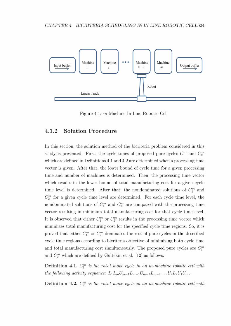
CHAPTER 4. BICRITERIA SCHEDULING IN IN-LINE ROBOTIC CELLS24
Input buffer Output bufferMachine
1
Machine
2
Machine Machine
Robot
Linear Track
1m − m
Figure 4.1: m-Machine In-Line Robotic Cell
4.1.2 Solution Procedure
In this section, the solution method of the bicriteria problem considered in this
study is presented. First, the cycle times of proposed pure cycles Cm1 and Cm
2
which are defined in Definitions 4.1 and 4.2 are determined when a processing time
vector is given. After that, the lower bound of cycle time for a given processing
time and number of machines is determined. Then, the processing time vector
which results in the lower bound of total manufacturing cost for a given cycle
time level is determined. After that, the nondominated solutions of Cm1 and
Cm2 for a given cycle time level are determined. For each cycle time level, the
nondominated solutions of Cm1 and Cm
2 are compared with the processing time
vector resulting in minimum total manufacturing cost for that cycle time level.
It is observed that either Cm1 or Cm
2 results in the processing time vector which
minimizes total manufacturing cost for the specified cycle time regions. So, it is
proved that either Cm1 or Cm
2 dominates the rest of pure cycles in the described
cycle time regions according to bicriteria objective of minimizing both cycle time
and total manufacturing cost simultaneously. The proposed pure cycles are Cm1
and Cm2 which are defined by Gultekin et al. [12] as follows:
Definition 4.1. Cm1 is the robot move cycle in an m-machine robotic cell with
the following activity sequence: L1LmUm−1Lm−1Um−2Lm−2 . . . U2L2U1Um.
Definition 4.2. Cm2 is the robot move cycle in an m-machine robotic cell with
CHAPTER 4. BICRITERIA SCHEDULING IN IN-LINE ROBOTIC CELLS25
the following activity sequence: L1UmLmUm−1Lm−1 . . . U2L2U1.
In the initial state of the cycle Cm1 , the machines 1 and m are idle and the
rest of the machines 2 to m − 1 are already loaded with a part. In the initial
state of the cycle Cm2 , only machine 1 is idle and the rest of the machines 2 to m
are loaded with a part.
The controllable processing times increase the solution flexibility such that
they result in at most equal cost to fixed processing times for a given cycle time
level K. The following example is useful to see the contribution of controllable
processing times, in order to decrease the total manufacturing cost, compared to
fixed processing times for cycle Cm2 . The total manufacturing cost of cycle Cm
2
with controllable processing times, which is studied in this study, is compared
to the total manufacturing cost of Cm2 in Gultekin et al. [12], where the pro-
cessing times on machines are assumed to be fixed and same for all machines. In
this example, we refer to some lemmas described in the further parts of this study.
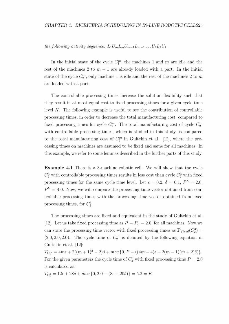
Example 4.1 There is a 3-machine robotic cell. We will show that the cycle
C32 with controllable processing times results in less cost than cycle C3
2 with fixed
processing times for the same cycle time level. Let ε = 0.2, δ = 0.1, PL = 2.0,
PU = 4.0. Now, we will compare the processing time vector obtained from con-
trollable processing times with the processing time vector obtained from fixed
processing times, for C32 .
The processing times are fixed and equivalent in the study of Gultekin et al.
[12]. Let us take fixed processing time as P = PL = 2.0, for all machines. Now we
can state the processing time vector with fixed processing times as Pfixed(C32) =
(2.0, 2.0, 2.0). The cycle time of Cm2 is denoted by the following equation in
Gultekin et al. [12]:
TCm2
= 4mε + 2((m + 1)2 − 2)δ + max{0, P − ((4m− 4)ε + 2(m− 1)(m + 2)δ)}For the given parameters the cycle time of C3
2 with fixed processing time P = 2.0
is calculated as:
TC32
= 12ε + 28δ + max{0, 2.0− (8ε + 20δ)} = 5.2 = K
CHAPTER 4. BICRITERIA SCHEDULING IN IN-LINE ROBOTIC CELLS26
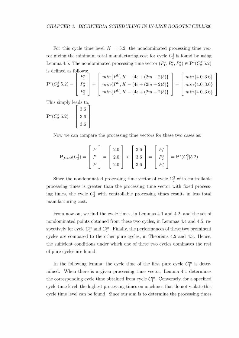
For this cycle time level K = 5.2, the nondominated processing time vec-
tor giving the minimum total manufacturing cost for cycle C32 is found by using
Lemma 4.5. The nondominated processing time vector (P ∗1 , P ∗
2 , P ∗3 ) ∈ P∗(C3
2 |5.2)
is defined as follows:
P∗(C32 |5.2) =
P ∗1
P ∗2
P ∗3
=
min{PU , K − (4ε + (2m + 2)δ)}min{PU , K − (4ε + (2m + 2)δ)}min{PU , K − (4ε + (2m + 2)δ)}
=
min{4.0, 3.6}min{4.0, 3.6}min{4.0, 3.6}
This simply leads to,
P∗(C32 |5.2) =
3.6
3.6
3.6
Now we can compare the processing time vectors for these two cases as:
Pfixed(C32) =
P
P
P
=
2.0
2.0
2.0
<
3.6
3.6
3.6
=
P ∗1
P ∗2
P ∗3
= P∗(C3
2 |5.2)
Since the nondominated processing time vector of cycle C32 with controllable
processing times is greater than the processing time vector with fixed process-
ing times, the cycle C32 with controllable processing times results in less total
manufacturing cost.
From now on, we find the cycle times, in Lemmas 4.1 and 4.2, and the set of
nondominated points obtained from these two cycles, in Lemmas 4.4 and 4.5, re-
spectively for cycle Cm1 and Cm
2 . Finally, the performances of these two prominent
cycles are compared to the other pure cycles, in Theorems 4.2 and 4.3. Hence,
the sufficient conditions under which one of these two cycles dominates the rest
of pure cycles are found.
In the following lemma, the cycle time of the first pure cycle Cm1 is deter-
mined. When there is a given processing time vector, Lemma 4.1 determines
the corresponding cycle time obtained from cycle Cm1 . Conversely, for a specified
cycle time level, the highest processing times on machines that do not violate this
cycle time level can be found. Since our aim is to determine the processing times

CHAPTER 4. BICRITERIA SCHEDULING IN IN-LINE ROBOTIC CELLS27
giving minimum manufacturing cost and since cost decreases as processing time
increases, this lemma is useful in finding the efficient set of solutions for Cm1 .
Lemma 4.1. The cycle time of Cm1 for a given processing time vector is found
as follows:
TCm1
= 4mε + 2m(m + 1)δ + max{0, P1− ((4m− 6)ε + 2(m2 − 2)δ), Pm − ((4m−6)ε + 2(m2 − 2)δ), Pkmax − ((4m− 4)ε + 2(m2 − 1)δ)}kmax = argmax{Pi : i ∈ [2, . . . , m− 1]}.
Proof. Gultekin et al. [12] defined the cycle time of Cm1 as the total time re-
quired for all of the robot activities and the waiting times in front of the machines
and denoted the cycle time as follows:
TCm1
= 4mε + (2m2 + 2m)δ + w1 + w2 + . . . + wm (4.1)
For an m-machine cell, the robot travel time between consecutive machines (δ),
the load/unload time of machines (ε), and the number of machines (m) are con-
stant. Thus, we only have to find the total waiting times in front of the machines
to calculate the cycle time. The time between loading machine i and the arrival
time of the robot in front of the machine i to unload it is denoted as vi. If
the processing time on machine i, Pi, exceeds vi, then the waiting time is the
difference between Pi and vi. Otherwise, the process on the machine is already
finished when the robot comes to machine i to unload it. Hence, the waiting time
of machine i is defined as wi = {0, Pi − vi}. We borrow the below definitions of
vi from Gultekin et al. [12].
v1 = TCm1−(6ε+(2m+4)δ+w1 +wm) = (4m−6)ε+(2m2−4)δ+w2 + . . .+wm−1.
vm = TCm1−(6ε+(2m+4)δ+wm) = (4m−6)ε+(2m2−4)δ+w1+w2+ . . .+wm−1.
In addition, the vi definition for i ∈ [2, . . . , m− 1] is presented as:
vi = TCm1− (4ε + (2m + 2)δ + wi) = (4m− 4)ε + (2m2− 2)δ + w1 + . . . + wm−wi.
If there is no waiting time on none of the machines, w1 + w2 + . . . + wm = 0.
If there is waiting time on machine 1, then:
w1 + w2 + . . . + wm = P1 − v1 +∑
j 6=1 wj = P1 − (4m− 6)ε− (2m2 − 4)δ + wm.
If there is waiting time on machine i where i ∈ [2, . . . ,m− 1], then:
w1 + w2 + . . . + wm = Pi − vi +∑
j 6=i wj = Pi − (4m− 4)ε− (2m2 − 2)δ.
If there is waiting time on machine m, then:

CHAPTER 4. BICRITERIA SCHEDULING IN IN-LINE ROBOTIC CELLS28
w1 + w2 + . . . + wm = Pm − vm +∑
j 6=m wj = Pm − (4m− 6)ε− (2m2 − 4)δ.
There are four different cases for the total waiting times and the sufficient condi-
tions for these cases are determined as follows:
1. If Pi ≤ vi, ∀i ∈ [1, . . . ,m], then wi = 0, for i = 1, . . . , m.
2. Else if Pkmax > vkmax , then wkmax = Pkmax − vkmax = Pkmax − (4m − 4)ε −(2m2− 2)δ−∑
i 6=kmaxwi. Hence, w1 +w2 + . . .+wm = Pkmax − (4m− 4)ε−
(2m2 − 2)δ.
3. Else if Pm > vm, then wm = Pm − vm = Pm − (4m − 6)ε − (2m2 − 4)δ −∑i6=m wi. Hence, w1 + w2 + . . . + wm = Pm − (4m− 6)ε− (2m2 − 4)δ.
4. Else if only P1 > v1, then wm = 0 and w1 = P1−v1 = P1−(4m−6)ε−(2m2−4)δ−∑
i6=1,m wi. Hence, w1 +w2 + . . .+wm = P1− (4m− 6)ε− (2m2− 4)δ.
As a consequence, total waiting time is calculated as:
w1 + w2 + . . . + wm = max{0, P1 − ((4m− 6)ε + (2m2 − 4)δ), Pm − ((4m− 6)ε +
(2m2 − 4)δ), Pkmax − ((4m− 4)ε + (2m2 − 2)δ)}.The cycle time of Cm
1 is obtained by replacing the total waiting time in the
equation (4.1) with this max function.
In Lemma 4.2, the cycle time of Cm2 is determined. When there is a given
processing time vector, Lemma 4.2 gives the corresponding cycle time. Similar to
Lemma 4.1, Lemma 4.2 can be used to determine the largest feasible processing
times for a given cycle time level.
Lemma 4.2. The cycle time of Cm2 for a given processing time vector is found
as follows:
TCm2
= 4mε+2((m+1)2−2)δ +max{0, Pkmax− ((4m−4)ε+2(m−1)(m+2)δ)},kmax = argmax{Pi : i ∈ [1, . . . , m]}.
Proof. Gultekin et al. [12] defined the cycle time of the second pure cycle
Cm2 as follows:
TCm2
= 4mε + (2m2 + 4m− 2)δ + w1 + w2 + . . . + wm. (4.2)

CHAPTER 4. BICRITERIA SCHEDULING IN IN-LINE ROBOTIC CELLS29
The total waiting time have to be found in order to calculate the cycle time of
Cm2 corresponding to a processing time. The waiting time on machine i is defined
as wi = {0, Pi − vi}. The definition of vi for all machines is identical for Cm2 and
it is presented by Gultekin et al. [12] as:
vi = TCm2−(4ε+(2m+2)δ+wi) = (4m−4)ε+2(m−1)(m+2)δ+w1+. . .+wm−wi.
If there is no waiting time on none of the machines, then w1 +w2 + . . .+wm = 0.
If there is some waiting time on some machine i, then:
w1 + w2 + . . . + wm = Pi− vi +∑
j 6=i wj = Pi− (4m− 4)ε− 2(m− 1)(m + 2)δ, ∀i.There are two different total waiting time results and the sufficient conditions for
these cases are determined as follows:
1. If Pi ≤ vi for ∀i ∈ [1, . . . , m], then wi = 0, for i = 1, . . . , m
2. Else if Pkmax > vkmax , then wkmax = Pkmax − vkmax = Pkmax − (4m − 4)ε −2(m− 1)(m + 2)δ−∑
i 6=kmaxwi. Hence, the total waiting time is as follows:
w1 + w2 + . . . + wm = Pkmax − ((4m− 4)ε + 2(m− 1)(m + 2)δ).
So, w1 + w2 + . . . + wm = max{0, Pkmax − (4m− 4)ε− 2(m− 1)(m + 2)δ} and the
cycle time is obtained by replacing the total waiting time in the equation (4.2)
with this max function.
In the next theorem, the lower bound for the cycle time of pure cycles with
controllable processing times is defined. The lower bound of cycle time for pure
cycles is determined by using Theorem 4.1, when a processing time vector is
given.
Theorem 4.1. For an m-machine robotic cell with controllable processing times,
the cycle time of any pure cycle is no less than
Tcontr = max{4mε + 2m(m + 1)δ, 4ε + (2m + 2)δ + max{Pi, i : 1, . . . ,m}}. (4.3)
Proof. From the definition of pure cycles, we determine that the cycle time
of a pure cycle has to be greater than or equal to two lower bounds. The first
lower bound is obtained from the exact robot activity time and the second one is
obtained from the given processing time vector. Since the robot has to perform an

CHAPTER 4. BICRITERIA SCHEDULING IN IN-LINE ROBOTIC CELLS30
exact set of robot activities, the total time required for these activities constitutes
a lower bound. Thus, the first lower bound is obtained as follows: The set of robot
activities can be analyzed in two groups, the first group consists of robot loading
and unloading times. First, a part is taken from the input buffer (ε) then loaded
to one of the machines (ε) after the processing on the machine is finished, the
part is unloaded (ε) and dropped to the output buffer (ε). This makes a total of
4mε time units for a cycle. The robot travel times constitute the second group
of robot activities. For any part, the robot takes the part from input buffer to
output buffer ((m+1)δ). Then, the robot travels from the output buffer to input
buffer to take a new part or to complete the cycle ((m+1)δ). This makes a total
of 2m(m + 1)δ time units for a cycle. Consequently, the first lower bound, which
is the total time required to complete the set of robot activities, makes a total of
4mε+2m(m + 1)δ.
The second lower bound is the minimum time between two consecutive load-
ings of any machine. The minimum time needed to unload machine i after loading
it is Pi time units. After the processing on the part is finished, it is unloaded (ε),
the part is transferred to output buffer ((m+1−i)δ), and the part is dropped (ε).
After that, the robot travels to the input buffer to take a new part to make the
consecutive loading of machine i ((m+1)δ), takes a new part part, (ε), brings the
new part to machine i (iδ) and finally loads the machine (ε). Hence, the minimum
time required between two consecutive loadings of machine i is 4ε+(2m+2)δ+Pi.
However there are m machines and the processing times on these machines may
be different from each other, due to controllability. Thus, the cycle time has to
be at least equal to the minimum time required between two consecutive load-
ings of any machine in the cell. So, the second lower bound of the cycle time is
4ε + (2m + 2)δ + max{Pi, i : 1, . . . , m}.
Our aim is to determine the processing time vector providing the minimum
cost for a given cycle time level. The total manufacturing cost depends only on
the processing times on machines. The manufacturing cost of a machine decreases
as the processing time increases on that machine. A feasible processing time must
satisfy PL ≤ Pi ≤ PU . Since PL constrains processing time from below and our
aim is to determine the largest feasible processing time vector, it is not necessary
CHAPTER 4. BICRITERIA SCHEDULING IN IN-LINE ROBOTIC CELLS31
to involve PL in analysis as a constraint. A processing time vector is composed of
processing times on machines constrained by two bounds. For any pure cycle, the
processing time on any machine is bounded above by the processing time upper
bound PU . In addition, from Theorem 4.1, processing times are bounded by cycle
time level K. Consequently, for a given cycle time level, we can find the upper
bounds of processing times for pure cycles that do not violate this cycle time level.
After obtaining these two bounds for processing times on all machines, the upper
bound of processing time vectors is determined for pure cycles. In other words,
any pure cycle cannot have a greater processing time vector than the proposed
processing time vector of the next lemma. Since this processing time vector is an
upper bound for the processing time vectors obtained from pure cycles for a cycle
time level K, it also results in the lower bound of total manufacturing cost that
a pure cycle can result in. Let P(K) = (P 1(K), . . . , Pm(K)) denote the upper
bound of processing time vectors. Now, P(K) for a given cycle time level K is
found as follows:
Lemma 4.3. For a given cycle time level K, the upper bound of processing time
vectors for pure cycles is represented as follows:
P(K) = (P 1(K), . . . , Pm(K)), where P i(K) = min{PU , K−(4ε+(2m+2)δ)},∀i.
Proof. The two bounds constraining processing time vectors are found in the
following cases.
1. The processing time on any machine is less than PU . This leads to:
P i(K) ≤ PU , ∀i.
2. In addition, the processing times on the machines cannot exceed a specific
value, since otherwise the cycle time level K will be exceeded. Now, we
find the upper bound of processing time on machine i, Pi, for the cycle time
level K. Theorem 4.1 determines the lower bound for the cycle time, when
a processing time vector is given. The cycle time lower bound in Theorem
4.1 is presented as:
Tcontr = max{4mε + 2m(m + 1)δ, 4ε + (2m + 2)δ + max{Pi, i : 1, . . . , m}}.
CHAPTER 4. BICRITERIA SCHEDULING IN IN-LINE ROBOTIC CELLS32
Let us set the cycle time K, then cycle time is at least equal to the cycle
time lower bound :
Tcontr = max{4mε+2m(m+1)δ, 4ε+(2m+2)δ+max{Pi, i : 1, . . . ,m}} ≤ K
Now, the processing time upper bound for machine i is found as follows:
max{Pi, i : 1, . . . , m} ≤ K−(4ε+(2m+2)δ), then Pi ≤ K−(4ε+(2m+2)δ,
∀i. This implies that P i(K) ≤ K − (4ε + (2m + 2)δ, ∀i.
Hence, the P(K) is upper bound of processing time vectors satisfying the two
bounds described above for a given cycle time level.
In order to compare the total manufacturing costs obtained from cycles Cm1
and Cm2 to the remaining pure cycles, we construct Lemmas 4.4 and 4.5, respec-
tively, to determine the processing times that give minimum total manufacturing
cost for a given cycle time level K. In order to decrease the total manufacturing
cost, the processing times have to take their maximum value without exceeding
bounds. There are two bounds constraining the processing times: the first con-
straint is the processing time upper bound (PU). The second constraint is the
cycle time (K) constraint. For a given cycle time level K, the processing times
are bounded such that the resulting cycle time value must not exceed this cy-
cle time level. In the following lemma, the set of nondominated processing time
vectors for cycle Cm1 , which is denoted as P∗(Cm
1 |K) is determined. The non-
dominated solutions in P∗(Cm1 |K) are the optimum solutions of corresponding
ECPs pertaining to cycle time level K. Let (P ∗1 , P ∗
2 , . . . , P ∗m) ∈ P∗(Cm
1 |K), be a
nondominated processing time vector. We can see from Lemma 4.1, the cycle Cm1
is feasible when the cycle time is 4mε + 2m(m + 1)δ ≤ K, and hence we consider
this region in the next lemma.
Lemma 4.4. Given any feasible cycle time level K, the nondominated processing
time vector (P ∗1 , P ∗
2 , . . . , P ∗m) ∈ P∗(Cm
1 |K) is defined as:

CHAPTER 4. BICRITERIA SCHEDULING IN IN-LINE ROBOTIC CELLS33
P∗(Cm1 |K) =
P ∗1
P ∗2...
P ∗m−1
P ∗m
=
min{PU , K − (6ε + (2m + 4)δ)}min{PU , K − (4ε + (2m + 2)δ)}
...
min{PU , K − (4ε + (2m + 2)δ)}min{PU , K − (6ε + (2m + 4)δ)}
Proof. The two upper bounds for processing times are presented as follows:
1. Any feasible processing time is at most equal to PU . Since (P ∗1 , P ∗
2 , . . . , P ∗m)
is also a feasible solution, then P ∗i ≤ PU , ∀i.
2. In addition, the processing times on machines cannot exceed a specific
amount, since the cycle time is bounded by level K. In Lemma 4.1, it
can be seen that cycle time depends on the processing times. Conversely,
the cycle time level K constrains the processing times so that they do not
exceed an upper bound. Now, we will find the processing times on machine
1 and m, e.g. P1 and Pm, respectively, for the cycle time level K. The
processing time upper bounds for cycle time level K are found by using
Lemma 4.1 as follows:
K = 4mε + 2m(m + 1)δ + max{0, P1 − ((4m − 6)ε + 2(m2 − 2)δ), Pm −((4m− 6)ε + 2(m2 − 2)δ), Pkmax − ((4m− 4)ε + 2(m2 − 1)δ)}, where
kmax = argmax{Pi : i ∈ [2, . . . , m− 1]}.We find that P1 ≤ K− (6ε+(2m+4)δ). Since P ∗
1 is also a feasible solution,
it has to satisfy this condition as well, hence P ∗1 ≤ K − (6ε + (2m + 4)δ).
Similarly, Pm ≤ K − (6ε + (2m + 4)δ), thus P ∗m ≤ K − (6ε + (2m + 4)δ).
In addition, we find that Pkmax ≤ K − (4ε + (2m + 2)δ), since Pi ≤ Pkmax
for i ∈ [2, . . . ,m − 1], then Pi ≤ K − (4ε + (2m + 2)δ). This simply leads
to P ∗i ≤ K − (4ε + (2m + 2)δ) for i ∈ [2, . . . , m− 1].
As a result, the processing time bounds pertaining to cycle time level K
are presented as follows:

CHAPTER 4. BICRITERIA SCHEDULING IN IN-LINE ROBOTIC CELLS34
P ∗1
P ∗2...
P ∗m−1
P ∗m
≤
K − (6ε + (2m + 4)δ)
K − (4ε + (2m + 2)δ)...
K − (4ε + (2m + 2)δ)
K − (6ε + (2m + 4)δ)
The processing times on their maximum values, without violating the bounds
found in the first and second arguments, compose the nondominated processing
time vectors stated in Lemma 4.4.
The next example is useful to understand the contribution of controllable
processing times in order to decrease the total manufacturing cost of cycle Cm1 .
Furthermore, we can see that the total manufacturing cost of nondominated so-
lution of Cm1 with controllability is less than the total manufacturing cost of
nondominated solution of Cm1 with fixed processing times.
Example 4.2 In this example, we will show that the cycle C41 with controllable
processing times results in less cost than C41 with fixed processing times, for a
4-machine robotic cell. Let ε = 0.2, δ = 0.1, PU = 6.5 and assume that the
cycle time level is K = 8.0. By using Lemma 4.4, for cycle time level K, the
nondominated processing time vector, (P ∗1 , P ∗
2 , P ∗3 , P ∗
4 ) ∈ P∗(C41 |8.0), giving the
minimum total manufacturing cost is found as follows:
P∗(C41 |8.0) =
P ∗1
P ∗2
P ∗3
P ∗4
=
min{PU , K − (6ε + (2m + 4)δ)}min{PU , K − (4ε + (2m + 2)δ)}min{PU , K − (4ε + (2m + 2)δ)}min{PU , K − (6ε + (2m + 4)δ)}
=
min{6.5, 5.6}min{6.5, 6.2}min{6.5, 6.2}min{6.5, 5.6}
This simply leads to:
P∗(C41 |8.0) =
5.6
6.2
6.2
5.6
Now, we will calculate the nondominated processing time vector for fixed
processing times in the study of Gultekin et al. [12]. The cycle time corresponding

CHAPTER 4. BICRITERIA SCHEDULING IN IN-LINE ROBOTIC CELLS35
to a fixed processing time P , on each machine, is found as:
TCm1
= 4mε + 2m(m + 1)δ + max{0, P − ((4m− 6)ε + 2(m2 − 2)δ)}
After a simple calculation we obtain P ≤ TCm1− 6ε− (2m + 4)δ.
Our cycle time level is K, we can replace TCm1
with K and the following result
is obtained:
P ≤ K−6ε−(2m+4)δ. For the given set of data in this example, P ≤ 5.6 for
all machines. Now we can state the nondominated processing time vector with
fixed processing times as P∗fixed(C
41 |8.0) = (5.6, 5.6, 5.6, 5.6).
The nondominated processing time vectors obtained from these two cases are
compared as follows:
P∗fixed(C
41 |8.0) =
P
P
P
P
=
5.6
5.6
5.6
5.6
≤
5.6
6.2
6.2
5.6
=
P ∗1
P ∗2
P ∗3
P ∗4
= P∗(C41 |8.0)
By comparing the processing times of P∗fixed(C
41 |8.0) and P∗(C4
1 |8.0), we see
that P = P ∗1 = P ∗
4 and P < P ∗2 = P ∗
3 . Thus, the nondominated processing time
vector of C41 with controllable processing times results in less total manufacturing
cost.
In the following lemma, we determine P∗(Cm2 |K), the set of nondominated
processing time vectors for cycle Cm2 that simultaneously minimize the cycle time
and the total manufacturing cost. It can be seen from Lemma 4.2 that the cycle
Cm2 is feasible when cycle time is 4mε + 2((m + 1)2 − 2)δ ≤ K, thus the ECP
problem is solved for cycle time level K in this boundary to construct the efficient
frontier.
Lemma 4.5. Given any feasible cycle time level K, the nondominated processing
time vector (P ∗1 , P ∗
2 , . . . , P ∗m) ∈ P∗(Cm
2 |K) is defined as follows:

CHAPTER 4. BICRITERIA SCHEDULING IN IN-LINE ROBOTIC CELLS36
P∗(Cm2 |K) =
P ∗1...
P ∗m
=
min{PU , K − (4ε + (2m + 2)δ)}...
min{PU , K − (4ε + (2m + 2)δ)}
Proof. For a given cycle time level K, a feasible processing time vector is
composed of processing times on machines that satisfy two upper bounds.
1. The processing times of a feasible processing time vector has to be at most
equal to PU . Since (P ∗1 , P ∗
2 , . . . , P ∗m) is also a feasible processing time vector,
then P ∗i ≤ PU , ∀i.
2. In addition, the processing times are bounded to satisfy the cycle time level
K. Now, we will determine the processing time on machine i, Pi, for the
cycle time K. By using Lemma 4.2 the cycle time level K can be presented
as follows:
K = 4mε+2((m+1)2−2)δ+max{0, Pkmax−((4m−4)ε+2(m−1)(m+2)δ)},kmax = argmax{Pi : i ∈ [1, . . . , m]}.This leads to Pkmax ≤ K−(4ε+(2m+2)δ). Since Pi ≤ Pkmax , it implies that
Pi ≤ K− (4ε+(2m+2)δ). Since P ∗i is feasible, P ∗
i ≤ K− (4ε+(2m+2)δ),
∀i.The processing time bounds pertaining to the cycle time level K are pre-
sented as follows:
P ∗1...
P ∗m
≤
K − (4ε + (2m + 2)δ)...
K − (4ε + (2m + 2)δ)
The processing times on their maximum values, without violating the bounds
found in the first and second arguments, compose the nondominated processing
time vectors stated in Lemma 4.5.
In the next two theorems, Theorems 4.2 and 4.3, we prove that the two promi-
nent pure cycles, Cm1 and Cm
2 , dominate the rest of pure cycles in the specified
regions. The feasible cycle time region of pure cycles obtained from Theorem 4.1

CHAPTER 4. BICRITERIA SCHEDULING IN IN-LINE ROBOTIC CELLS37
is 4mε+2m(m+1)δ ≤ K. We analyze this cycle time region in two parts. The first
region is where the cycle Cm2 is feasible and the second region is where the cycle
Cm2 is not feasible but Cm
1 is feasible. We can see from Lemma 4.2 that the cycle
Cm2 is feasible when cycle time is 4mε + 2((m + 1)2 − 2)δ ≤ K. In Theorem 4.2,
we show that pure cycle Cm2 dominates the rest of pure cycles in this region. In
addition, from Theorem 4.1, the cycle time lower bound that can be attained from
pure cycles is 4mε+2m(m+1)δ. We can see that the only region that Cm2 is not
feasible is the cycle time region 4mε+2m(m+1)δ ≤ K < 4mε+2((m+1)2−2)δ.
In Theorem 4.3, we show that Cm1 dominates the rest of pure cycles under spec-
ified conditions, in this region. So, it is seen that the proposed pure cycles Cm1
and Cm2 dominate rest of the pure cycles in most of the regions. In the following
theorem, we prove that the second pure cycle Cm2 dominates the rest of the pure
cycles in the described region. We see that the cycle Cm2 results in the lower
bound of total manufacturing cost in the specified region. Since the lower bound
of total manufacturing cost corresponds to the upper bound of processing time
vectors, we show that Cm2 results in the upper bound of processing time vectors,
for the cycle time level K. From Lemma 4.2, Cm2 is feasible when cycle time
is 4mε + 2((m + 1)2 − 2)δ ≤ K, thus we consider this cycle time region in the
following theorem.
Theorem 4.2. Whenever Cm2 is feasible, it dominates all other pure cycles.
There are two possible cases that may arise according to processing time upper
bound PU .
1. The first case considers that PU ≤ K − (4ε + (2m + 2)δ). The nondomi-
nated processing time vector for cycle Cm2 is determined by using Lemma
4.5. Take any nondominated solution (P ∗1 , P ∗
2 , . . . , P ∗m) ∈ P∗(Cm
2 |K). The
processing time of machine i, P ∗i is found by using Lemma 4.5 such
that P ∗i = min{PU , K − (4ε + (2m + 2)δ)}. Since we assumed that
PU ≤ K − (4ε + (2m + 2)δ), then P ∗i = PU . We can present the non-
dominated processing time vector of Cm2 as follows:
(P ∗1 , P ∗
2 , . . . , P ∗m) = (PU , PU , . . . , PU)

CHAPTER 4. BICRITERIA SCHEDULING IN IN-LINE ROBOTIC CELLS38
The upper bound of processing time vectors found by using Lemma 4.3 is
presented as:
P(K) = (P 1(K), P 2(K), . . . , Pm(K)) = (PU , PU , . . . , PU).
The processing time vector obtained from Cm2 is equal to the upper bound
of processing time vectors for cycle time level K, P∗(Cm2 |K) = P(K), Since
all processing times take the maximum value PU , there is not any other
pure cycle that can result in smaller total manufacturing cost.
2. The second possible case for the processing time upper bound is:
PU > K − (4ε + (2m + 2)δ).
The nondominated processing time vector of Cm2 is found from Lemma 4.5
as follows:
P∗(Cm2 |K) =
P ∗1...
P ∗m
=
K − (4ε + (2m + 2)δ)...
K − (4ε + (2m + 2)δ)
The upper bound of processing time vectors found by using Lemma 4.3 is
presented as follows:
P(K) = (P 1(K), . . . , Pm(K)) where P i(K) = K − (4ε + (2m + 2)δ), ∀i.The processing time vector obtained from the cycle Cm
2 is equal to the up-
per bound of processing time vectors for this cycle time level, P∗(Cm2 |K) =
P(K), thus there is not any pure cycle that can result in less total manu-
facturing cost.
In the next theorem, we prove that Cm1 dominates the rest of the pure cycles
in the described region, under the specified condition. Since the lower bound
of total manufacturing cost corresponds to the upper bound of processing time
vectors, we show that Cm1 results in the upper bound of processing time vectors.
Cm1 is found to be feasible when cycle time is 4mε + 2m(m + 1)δ ≤ K by using
Lemma 4.1. In addition, in Theorem 4.2, we show that Cm2 dominates all of the
other pure cycles when cycle time is 4mε + 2((m + 1)2 − 2)δ ≤ K. Now, we will
show that Cm1 dominates the rest of the pure cycles in the remaining cycle time
region; 4mε + 2m(m + 1)δ ≤ K < 4mε + 2((m + 1)2 − 2)δ under the specified
condition of PU .
CHAPTER 4. BICRITERIA SCHEDULING IN IN-LINE ROBOTIC CELLS39
Theorem 4.3. For the remaining region 4mε+2m(m+1)δ ≤ K < 4mε+2((m+
1)2 − 2)δ, Cm1 dominates the rest of pure cycles if PU ≤ K − (6ε + (2m + 4)δ).
Proof. In this case, we consider that PU ≤ K − (6ε + (2m + 4)δ). The
nondominated processing time vector for cycle Cm1 is found by Lemma 4.4. Take
any nondominated processing time vector (P ∗1 , P ∗
2 , . . . , P ∗m) ∈ P∗(Cm
1 |K). We
find the processing time of machine 1, P ∗1 , as an example. From Lemma 4.4,
P ∗1 = min{PU , K − (6ε + (2m + 4)δ)} and since, PU ≤ K − (6ε + (2m + 4)δ) is
assumed, we have P ∗1 = PU . Similarly, we find all of the other processing times of
nondominated processing time vector of Cm1 and the following result is obtained:
(P ∗1 , P ∗
2 , . . . , P ∗m) = (PU , PU , . . . , PU)
In addition, from Lemma 4.3, we find the upper bound of processing time
vectors as follows:
P(K) = (P 1(K), P 2(K), . . . , Pm(K)) = (PU , PU , . . . , PU).
The processing time vector obtained from Cm2 is equal to the upper bound of
processing time vectors P∗(Cm1 |K) = P(K). Since all the processing times on
the machines take the maximum value, PU , there is not any other pure cycle that
can result in less total manufacturing cost.
In the next lemma, we compare the total manufacturing cost of pure cycle
Cm1 with the lower bound of total manufacturing cost. The region considered in
Lemma 4.6 is the only region where neither Cm1 nor Cm
2 dominates the rest of the
pure cycles. Since Cm1 is feasible and Cm
2 is not feasible in this region, only Cm1 is
considered. The term F1(Cm1 ,P∗(Cm
1 |K)) denotes the total manufacturing cost
incurred by nondominated processing time vector of the cycle Cm1 for the given
cycle time level K. Similarly, the term FLB1 (Cm
i ,P(K)) denotes the lower bound
of total manufacturing cost of pure cycles for the given cycle time level K. We
present the performance analysis below in which f(χ) gives the manufacturing
cost when the processing time is equal to χ.
Lemma 4.6. For the remaining region 4mε + 2m(m + 1)δ ≤ K < 4mε + 2((m +
1)2 − 2)δ and K − (6ε + (2m + 4)δ) < PU , the performance of the cycle Cm1 in

CHAPTER 4. BICRITERIA SCHEDULING IN IN-LINE ROBOTIC CELLS40
this region is stated as below:
F1(Cm1 ,P∗(Cm
1 |K)) ≤ FLB1 (Cm
i ,P(K)).%, where % = (1− 2m
+2f((4m−6)ε+2(m2−2)δ)mf((4m−4)ε+2(m2−1)δ)
).
Proof. We analyze the performance in two regions according to the level of
processing time upper bound PU .
1. First, we consider the case where :
K − (6ε + (2m + 4)δ) < PU ≤ K − (4ε + (2m + 2)δ).
Take any nondominated processing time vector (P ∗1 , P ∗
2 , . . . , P ∗m) ∈
P∗(Cm1 |K). Now we will determine the processing time on machine 1, P ∗
1 , as
an example. Lemma 4.4 implies that P ∗1 = min{PU , K− (6ε+(2m+4)δ)}.
Since we assumed that K − (6ε + (2m + 4)δ) < PU , the processing time on
this machine is P ∗1 = K − (6ε + (2m + 4)δ). Similarly, all processing times
of P∗(Cm1 |K) are found and the following result is obtained:
P∗(Cm1 |K) =
P ∗1
P ∗2...
P ∗m−1
P ∗m
=
K − (6ε + (2m + 4)δ)
PU
...
PU
K − (6ε + (2m + 4)δ)
We compare the total manufacturing cost of P∗(Cm1 |K) to the lower bound
of total manufacturing cost which corresponds to the upper bound of pro-
cessing time vectors for the cycle time level K and the upper bound of
processing time vectors is found from Lemma 4.3 as follows:
P(K) = (P 1(K), P 2(K), . . . , Pm(K)) = (PU , PU , . . . , PU).
The total manufacturing cost obtained from P∗(Cm1 |K) is equal to the total
of manufacturing costs on machines and it is calculated as follows:
F1(Cm1 ,P∗(Cm
1 |K)) = (m− 2)f(PU) + 2f(K − (6ε + (2m + 4)δ)).
The lower bound of total manufacturing cost for cycle time level K is found
as:
FLB1 (Cm
i ,P(K)) =∑m
i=1 f(Pi) = mf(PU).

CHAPTER 4. BICRITERIA SCHEDULING IN IN-LINE ROBOTIC CELLS41
Now, we can calculate the performance by dividing the total manufacturing
cost obtained from cycle Cm1 to the lower bound of total manufacturing cost.
F1(Cm1 ,P∗(Cm
1 |K))
F LB1 (Cm
i ,P(K))=
(m−2)f(P U)+2f(K−(6ε+(2m+4)δ))mf(P U)
= 1− 2m
+2f(K−(6ε+(2m+4)δ))
mf(P U).
In this case PU ≤ K − (4ε + (2m + 2)δ) is assumed. Hence, we have the
following:
2f(K−(6ε+(2m+4)δ))mf(P U)
≤ 2f(K−(6ε+(2m+4)δ))mf(K−(4ε+(2m+2)δ))
We assumed that 4mε + 2m(m + 1)δ ≤ K, then we can say that:
2f(K−(6ε+(2m+4)δ))mf(K−(4ε+(2m+2)δ))
≤ 2f((4m−6)ε+2(m2−2)δ)mf((4m−4)ε+2(m2−1)δ)
, thus
F1(Cm1 ,P∗(Cm
1 |K))
F LB1 (Cm
i ,P(K))≤ 1− 2
m+
2f((4m−6)ε+2(m2−2)δ)mf((4m−4)ε+2(m2−1)δ)
.
2. Now, we consider the second case where we assume that:
K − (4ε + (2m + 2)δ) < PU .
Take any nondominated processing time vector (P ∗1 , P ∗
2 , . . . , P ∗m) ∈
P∗(Cm1 |K). Now, we will determine the processing time on machine 2,
P ∗2 , as an example. From Lemma 4.4, we know that P ∗
2 = min{PU , K −(4ε + (2m + 2)δ)}. Since K − (4ε + (2m + 2)δ) < PU , the processing time
on that machine is P ∗2 = K − (4ε + (2m + 2)δ). Similarly, we find all of the
other processing times of P∗(Cm1 |K) by using Lemma 4.4 and the following
result is obtained:
P∗(Cm1 |K) =
P ∗1
P ∗2...
P ∗m−1
P ∗m
=
K − (6ε + (2m + 4)δ)
K − (4ε + (2m + 2)δ)...
K − (4ε + (2m + 2)δ)
K − (6ε + (2m + 4)δ)
We compare the total manufacturing cost of P∗(Cm1 |K) to the lower bound
of total manufacturing cost. The upper bound of processing time vector is
found from Lemma 4.3 as:
P(K) = (P 1(K), . . . , Pm(K)),
where P i(K) = min{PU , K − (4ε + (2m + 2)δ)}, ∀i.

CHAPTER 4. BICRITERIA SCHEDULING IN IN-LINE ROBOTIC CELLS42
Now, let us compare the total manufacturing cost of P∗(Cm1 |K) to the
lower bound of total manufacturing cost obtained from P(K) for given
cycle time level K. The total manufacturing cost obtained from P∗(Cm1 |K)
is calculated as follows:
F1(Cm1 ,P∗(Cm
1 |K)) = (m−2)f(K−(4ε+(2m+2)δ))+2f(K−(6ε+(2m+
4)δ)).
The lower bound of total manufacturing cost is found as:
FLB1 (Cm
i ,P(K)) =∑m
i=1 f(Pi) = mf(K − (4ε + (2m + 2)δ)).
Now, we can calculate the performance of Cm1 by dividing the total manu-
facturing cost obtained from cycle Cm1 to the lower bound.
F1(Cm1 ,P∗(Cm
1 |K))
F LB1 (Cm
i ,P(K))=
(m−2)f(K−(4ε+(2m+2)δ))+2f(K−(6ε+(2m+4)δ))mf(K−(4ε+(2m+2)δ))
= 1− 2m
+2f(K−(6ε+(2m+4)δ))mf(K−(4ε+(2m+2)δ))
We assumed that 4mε + 2m(m + 1)δ ≤ K, then we can say that:
2f(K−(6ε+(2m+4)δ))mf(K−(4ε+(2m+2)δ))
≤ 2f((4m−6)ε+2(m2−2)δ)mf((4m−4)ε+2(m2−1)δ)
, thus
F1(Cm1 ,P∗(Cm
1 |K))
F LB1 (Cm
i ,P(K))≤ 1− 2
m+
2f((4m−6)ε+2(m2−2)δ)mf((4m−4)ε+2(m2−1)δ)
In the previous lemma, the total manufacturing cost obtained from nondominated
solutions of the cycle Cm1 is compared with the lower bound of total manufactur-
ing cost obtained from Lemma 4.3. As can be seen from the statement in Lemma
4.6, the number of machines directly effects the difference in between the total
manufacturing cost of Cm1 and the lower bound of total manufacturing cost that
we could obtain for any pure cycle. The next example presents two cases which
are useful in understanding Lemma 4.6. In this example, we consider 2-machine
robotic cell case and an m-machine case where m →∞. The first case represents
the highest difference rate between the lower bound and the total manufacturing
cost of Cm1 . In the second case, the total manufacturing cost of Cm
1 becomes
equal to the lower bound. The cost function used in the next two examples is

CHAPTER 4. BICRITERIA SCHEDULING IN IN-LINE ROBOTIC CELLS43
modified from the cost functions given in Kayan and Akturk [21]. The opera-
tion to be performed on identical parts is a single pass turning operation using a
single cutting tool on identical CNC machines. The total manufacturing cost is
the sum of manufacturing costs on each machine, thus we define the machining
cost and the tooling cost on each machine. The machining cost for machine i is
defined as O.Pi where O is the operating cost which is identical for all machines.
The tooling cost on machine i is defined as TUP αi , where T > 0 and α < 0 are
constants for identical tools and U > 0 is a specific constant for identical oper-
ations on identical tools. Consequently, the manufacturing cost for machine i is
f(Pi) = O.Pi + TUP αi .
Example 4.3 In this example, we show that Cm1 performs better as the number
of machines increases. The total manufacturing cost of Cm1 gets closer to the
lower bound of total manufacturing cost as the number of machines increases.
Hence, we consider the case with infinite number of machines, where the total
manufacturing cost of Cm1 equals to the lower bound. Similarly, the difference
between the total manufacturing cost of Cm1 and the lower bound increases as the
number of machines decreases. In order to demonstrate this case, we consider the
two machine case. Let δ = 0.1, ε = 0.1, α = −1.2423, T = 1, U = 1, and O = 1.
The cost function corresponding to processing times on machines is described as
f(Pi) = O.Pi + TUP αi .
The performance measure for 2-machine case is calculated as % = 1.24 by
using Lemma 4.6. Thus, F1(C21 ,P
∗(C21 |K)) ≤ FLB
1 (C2i ,P(K)).(1.24). This state-
ment implies that Cm1 results in at most 1.24 times of the lower bound. In
addition, the minimum difference in performance occurs for m-machine case
where m → ∞. The performance difference is measured as % = 1 by using
Lemma 4.6. Thus, F1(Cm1 ,P∗(Cm
1 |K)) ≤ FLB1 (Cm
i ,P(K)). Since the total man-
ufacturing cost obtained from cycle Cm1 cannot be less than the lower bound,
F1(Cm1 ,P∗(Cm
1 |K)) = FLB1 (Cm
i ,P(K)). Hence, we see that the cycle Cm1 per-
forms better as the number of machines increases.
The next example presents the efficient frontiers of cycles Cm1 and Cm
2 for
given parameters and illustrates Theorem 4.2 and Lemma 4.6. We will see the

CHAPTER 4. BICRITERIA SCHEDULING IN IN-LINE ROBOTIC CELLS44
region where Cm2 dominates the rest of pure cycles. Furthermore, Cm
1 covers the
region where cycle Cm2 is not feasible and in that region, the performance analysis
of Cm1 is made by using Lemma 4.6.
�������������� ��� ��� � ���
���4
1C
4���� ��������������� ����� ����4
2C
Figure 4.2: C41 and C4
2 pure cycles
Example 4.4 In this example, we consider a turning operation with machines
using the same tool to produce identical parts in a 4-machine robotic cell. For
this turning operation, let the parameters be given as follows: T = 0.1, O = 0.1,
U = 1, α = −1.6423, ε = 0.02, δ = 0.01 and PU = 0.90.
The two curves in Figure 4.2 represent the efficient frontiers of C41 and C4
2 ,
which are constructed by using Lemmas 4.4 and 4.5 respectively. In this figure,
4mε + 2((m + 1)2 − 2)δ = 0.78 is the point found from Lemma 4.2 where C42
becomes feasible. It can be seen that C42 is presented in bold line, from Theorem
4.2, C42 dominates the rest of pure cycles when the cycle time is at least 0.78. In
addition, 4mε + 2m(m + 1)δ = 0.72 is the point where C41 becomes feasible. The
only region where C42 is not feasible is the cycle time region 0.72 ≤ K < 0.78. In
this region, the cycle C41 is feasible. Since K − (6ε + (2m + 4)δ) < PU in this
region, we cannot say that C41 dominates the rest of pure cycles by using Theorem
4.3. However, by using Lemma 4.6, we can calculate the performance of C41 in

CHAPTER 4. BICRITERIA SCHEDULING IN IN-LINE ROBOTIC CELLS45
this region as follows:
We find % = 1.08, by using Lemma 4.6. Hence, the total manufacturing cost
obtained from cycle C41 is at most 0.08 percent higher than the lower bound of
total manufacturing cost, in this region. As a result, we can conclude that C42
dominates the rest of pure cycles in most of the regions. In the only region where
C42 is not feasible, we see that the difference between the performance of C4
1 and
the lower bound is less than 0.08 times of the lower bound.
4.1.3 Discussion
The minimization of cycle time and minimization of total manufacturing cost
objectives are fundamental objectives in the scheduling literature. In this section,
we analyzed both of these objectives simultaneously in in-line robotic cells. The
problem is to find the robot move sequence and processing times on machines
minimizing the cycle time and the total manufacturing cost. In this section,
the robot move cycles Cm1 and Cm
2 are proved to be efficient in most of the cycle
time region according to the bicriteria objective. In the next section the optimum
number of machines in the cell is determined for Cm1 and Cm
2 as a design problem.
4.2 Optimum Number of Machines
Until now, we have dealt with operational problems in robotic cells. In this
section, we solve a design problem where we consider the number of machines as
a decision variable.
4.2.1 Problem Definition and Solution Procedure
The optimum number of machines which is useful to determine the equipment
requirements of the cell is calculated when the cycle time, robot travel times,
CHAPTER 4. BICRITERIA SCHEDULING IN IN-LINE ROBOTIC CELLS46
loading/unloading times and the processing time upper bound are given param-
eters. The following theorem determines the optimum number of machines for
Cm1 for the given values of ε, δ, the cycle time K, and PU .
Theorem 4.4. For a given cycle time K, the optimum number of machines m∗
for cycle Cm1 is one of the integers below giving less unit cycle time:
bmin{√
ε2 + δPU/2 + 3εδ + 2δ2−ε,√
ε2 + δK/2 + εδ + δ2/4−ε−δ/2}/δc or
bmin{√
ε2 + δPU/2 + 3εδ + 2δ2−ε,√
ε2 + δK/2 + εδ + δ2/4−ε−δ/2}/δc+1.
Proof. Lemma 4.4 defines the nondominated processing time vector of Cm1 as
(P ∗1 , P ∗
2 , . . . , P ∗m) ∈ P∗(Cm
1 |K) where P ∗1 = P ∗
m = min{PU , K− (6ε+(2m+4)δ)}and P ∗
2 = . . . = P ∗m−1 = min{PU , K − (4ε + (2m + 2)δ)}. The cycle time of Cm
1
for this processing time vector is found by using Lemma 4.1 as follows:
4mε+2m(m+1)δ+max{0, min{PU , K−(6ε+(2m+4)δ)}−((4m−6)ε+2(m2−2)δ)}
The per unit cycle time of Cm1 at cycle time K is found by dividing the cycle time
by m as follows:
max{4ε + (2m + 2)δ,min{PU + 6ε + (2m + 4)δ,K}/m}. (4.4)
In order to minimize per unit cycle time in equation (4.4), the two arguments in
the max function have to be minimized. The minimum value of max function is
the minimum value of two arguments or the intersection point of these two ar-
guments. As the number of machines decreases, the first argument decreases but
the second argument increases. The first argument takes its minimum value when
m = 0 but then the second argument min{PU + 6ε + (2m + 4)δ,K}/m →∞, so
it does not minimize the max function. The second argument takes its minimum
value when m →∞. However, when m →∞, the first term 4ε+(2m+2)δ →∞,
thus this does not give the minimum value of the max function. Now, we will
determine the only remaining minimizer of max function which is the intersection
of the two arguments:
4ε + (2m + 2)δ = min{PU + 6ε + (2m + 4)δ,K}/m.
This equation leads to:
CHAPTER 4. BICRITERIA SCHEDULING IN IN-LINE ROBOTIC CELLS47
min{PU + 6ε + 4δ − (2δm2 + 4εm), K − (2δm2 + (4ε + 2δ)m)} = 0.
This min function results 0 if the two arguments in the min function are non-
negative and one of them is equal to 0. The m values making these arguments
nonnegative are found as follows:
1. The first argument is nonnegative when:
0 ≤ PU + 6ε + 4δ − (2δm2 + 4εm).
This inequality has two roots and one of them is negative, we only consider
the positive root hence, the inequality holds when:
m ≤ (√
ε2 + δPU/2 + 3εδ + 2δ2 − ε)/δ.
2. The second argument is nonnegative when:
0 ≤ K − (2δm2 + (4ε + 2δ)m).
This inequality has two roots and one of them is negative, we only consider
the positive root hence the inequality holds when:
m ≤ (√
ε2 + δK/2 + εδ + δ2/4− ε− δ/2)/δ.
Since, both of the two arguments in the min function have to be nonnegative and
one of the arguments has to be 0, the optimum m is stated as follows:
m = min{(√
ε2 + δPU/2 + 3εδ + 2δ2−ε)/δ, (√
ε2 + δK/2 + εδ + δ2/4−ε−δ/2)/δ}
This equation may result in a fractional value but m∗ is an integer, thus m∗ is
the upper rounded or the lower rounded values of the equation above which gives
less per unit cycle time.
The following theorem determines m∗ of Cm2 for the given values of ε, δ, K,
and PU .
Theorem 4.5. For a given cycle time K, the optimum number of machines m∗
for cycle Cm2 is one of the integers below giving less unit cycle time:
bmin{√
ε2 + δPU/2 + 3εδ + 9δ2/4−ε−δ/2,√
ε2 + δK/2 + 2εδ + 2δ2−ε−δ}/δcor
bmin{√
ε2 + δPU/2 + 3εδ + 9δ2/4−ε−δ/2,√
ε2 + δK/2 + 2εδ + 2δ2−ε−δ}/δc+1.

CHAPTER 4. BICRITERIA SCHEDULING IN IN-LINE ROBOTIC CELLS48
Proof. Lemma 4.5 defines the nondominated processing time vector of Cm2
as (P ∗1 , P ∗
2 , . . . , P ∗m) ∈ P∗(Cm
2 |K) where P ∗1 = . . . = P ∗
m = min{PU , K − (4ε +
(2m + 2)δ)}. The per unit cycle time of Cm2 is found by dividing the cycle time
corresponding to the nondominated processing time vector, which is found by
using Lemma 4.2, by m as follows:
max{4ε + (2m + 4− 2/m)δ,min{PU + 4ε + (2m + 2)δ,K}/m}. (4.5)
In order to minimize per unit cycle time in equation (4.5), the two arguments in
the max function have to be minimized. The minimum value of max function
is the minimum value of two arguments or the intersection point of these two
arguments. As the number of machines decreases, the first argument decreases
but the second argument increases. The first argument becomes minimum when
m = 0 but then the second argument min{PU + 4ε + (2m + 2)δ,K}/m → ∞.
Hence, it does not minimize the max function. The second argument takes
its minimum value when m → ∞. However, when m → ∞, the first term
4ε + (2m + 4 − 2/m)δ → ∞. Thus, this does not give the minimum value of
the max function. Now, we will find the only remaining minimizer of the max
function which is the intersection of the two arguments:
4ε + (2m + 4− 2/m)δ = min{PU + 4ε + (2m + 2)δ,K}/m.
This equation leads to:
min{PU +4ε+4δ− (2δm2 +(4ε+2δ)m), K +2δ− (2δm2 +(4ε+4δ)m)} = 0.
This min function results 0 if the two arguments in the min function are non-
negative and one of them is equal to 0. The m values making these arguments
nonnegative are found as follows:
1. The first argument is nonnegative when:
0 ≤ PU + 4ε + 4δ − (2δm2 + (4ε + 2δ)m).
This inequality has two roots and one of them is negative, we only consider
the positive root. Hence, the inequality holds when:
m ≤ (√
ε2 + δPU/2 + 3εδ + 9δ2/4− ε− δ/2)/δ.
2. The second argument is nonnegative when:
0 ≤ K + 2δ − (2δm2 + (4ε + 4δ)m).

CHAPTER 4. BICRITERIA SCHEDULING IN IN-LINE ROBOTIC CELLS49
This inequality has two roots and one of them is negative. We only consider
the positive root. Hence, the inequality holds when:
m ≤ (√
ε2 + δK/2 + 2εδ + 2δ2 − ε− δ)/δ.
Since, both of the two arguments in the min function have to be nonnegative and
one of the arguments has to be 0, the optimum m is stated as follows:
min{(√
ε2 + δPU/2 + 3εδ + 9δ2/4−ε−δ/2)/δ, (√
ε2 + δK/2 + 2εδ + 2δ2−ε−δ)/δ}
This equation may result in a fractional value but m∗ is an integer, thus m∗ is
the upper rounded or the lower rounded values of the equation above which gives
less per unit cycle time.
We will now conclude the section by discussing the results found.
4.2.2 Discussion
Another problem focused in the literature is a design problem of finding the
optimum number of machines in the cell. In this section, we focus on the design
of the cell. The problem to be solved is to determine the optimum number of
machines for pure cycles Cm1 and Cm
2 in the cell when the robot load/unload times
and robot travel time are given parameters. Finally, we determined the optimum
number of machines for the two pure cycle studied in this chapter for Cm1 and
Cm2 .

Chapter 5
Pure Cycles in Robot Centered
Cells
In the previous chapter, we considered the minimization of cycle time and min-
imization of total manufacturing cost simultaneously for pure cycles in in-line
robotic cells. In this chapter, we analyze the pure cycles in a different cell layout.
The cell layout considered in this chapter is the robot centered cell. This chapter
is composed of two sections. In the first section, we determine the pure cycles
resulting in minimum cycle time for the described processing time regions. It is
assumed that the processing times on machines are fixed and the same for all
machines. We propose two cycles that are efficient in order to minimize the cycle
time. After that, we analyze the 3-machine case in order to find the processing
time regions and the corresponding pure cycles resulting in minimum cycle time
in these regions. In the second section, the processing times are assumed to be
controllable which makes our problem closer to the real life problems. We propose
that the same two pure cycles proposed in the first section result in the minimum
cycle time and minimum total manufacturing cost for most of the region. The
reason for this prediction is the efficiency of these cycles in order to minimize cy-
cle time. After that, the 3-machine robot centered cell is analyzed to determine
the pure cycles resulting in minimum cycle time and total manufacturing cost,
and the corresponding cycle time regions. Finally, the summary and the results
50

CHAPTER 5. PURE CYCLES IN ROBOT CENTERED CELLS 51
of this section are presented.
5.1 Minimizing Cycle Time with Fixed
Processing Times
In this problem, we considered an m-machine robot centered cell composed of
CNC machines and an output and an input buffer are combined in an I/O station.
In the first part, the problem to be solved is a single objective problem where the
objective is to minimize the cycle time. For this problem, the processing times
are assumed to be fixed and identical for all machines. We find the lower bound
of cycle time of pure cycles in robot centered cells for a given processing time.
We propose two pure cycles that result in the minimum cycle time in a specified
processing time region. For the remaining processing time region, the worst case
performance of these two pure cycles is determined. After that, the 3-machine
case is analyzed. It is observed that the proposed cycles results in the minimum
cycle time in most of the processing time region.
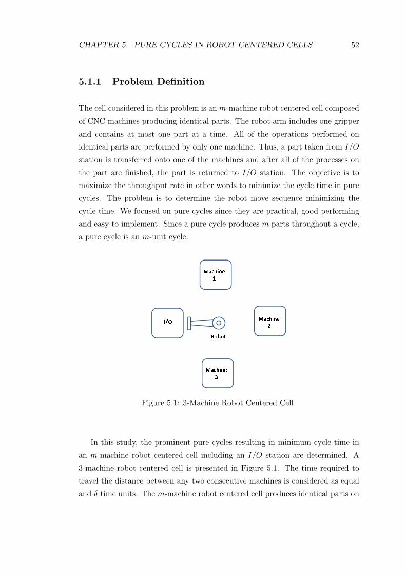
CHAPTER 5. PURE CYCLES IN ROBOT CENTERED CELLS 52
5.1.1 Problem Definition
The cell considered in this problem is an m-machine robot centered cell composed
of CNC machines producing identical parts. The robot arm includes one gripper
and contains at most one part at a time. All of the operations performed on
identical parts are performed by only one machine. Thus, a part taken from I/O
station is transferred onto one of the machines and after all of the processes on
the part are finished, the part is returned to I/O station. The objective is to
maximize the throughput rate in other words to minimize the cycle time in pure
cycles. The problem is to determine the robot move sequence minimizing the
cycle time. We focused on pure cycles since they are practical, good performing
and easy to implement. Since a pure cycle produces m parts throughout a cycle,
a pure cycle is an m-unit cycle.
������������ �������� ����������������
Figure 5.1: 3-Machine Robot Centered Cell
In this study, the prominent pure cycles resulting in minimum cycle time in
an m-machine robot centered cell including an I/O station are determined. A
3-machine robot centered cell is presented in Figure 5.1. The time required to
travel the distance between any two consecutive machines is considered as equal
and δ time units. The m-machine robot centered cell produces identical parts on

CHAPTER 5. PURE CYCLES IN ROBOT CENTERED CELLS 53
identical machines and the processing times of identical parts are assumed to be
fixed as P . The definitions and assumptions presented in Chapter 3 are used in
this section. Additional definitions used in this section and which are common in
literature is presented as follows:
δ : The time required for rotational movement between two consecutive ma-
chines which is assumed to be additive such that the travelling time between
machine i and j is min{|i− j|,m + 1− |i− j|}δ.
P : The fixed processing time on machines. The processing time is fixed and
the same for every machine in this section.
I/O station: The I/O station consists of an Input device, from which parts are
introduced into the cell, and an Output device, onto which the parts are
dropped upon completion of their processing on the machines
In the next section, the solution of the problem considered in this section is
presented.
5.1.2 Solution Procedure
In this part, the solution method of determining the pure cycles minimizing the
cycle time is presented step by step. At first, the intuition of finding good per-
forming pure cycles is presented. The number of different pure cycles is (2m−1)!
for an m-machine cell. For a 3-machine robotic cell, there are 120 pure cycles and
for a 4-machine robotic cell, there are 5040 pure cycles. The number of possible
pure cycles increases as a factorial function of the number of machines in the cell.
So it is very useful to have an intuition to find good performing cycles among
these numerous cycles. Furthermore, the cycles we proposed according to this
intuition are proved to minimize cycle time as will be shown in the later parts
of this study. After presenting the intuition of selecting good pure cycles among
numerous pure cycles, we propose that two pure cycles are efficient cycles. Then,
the cycle times of these pure cycles are determined when there is a given pro-
cessing time. The lower bound of cycle time is found for the robot centered cell.
CHAPTER 5. PURE CYCLES IN ROBOT CENTERED CELLS 54
Consequently, the cycle times obtained from the proposed cycles are compared to
the lower bound of cycle time and by this way, the processing time region where
the proposed cycles result in minimum cycle time is determined. After that, the
3-machine analysis is presented.
5.1.2.1 Intuition for Efficient Pure Cycles
At this step, the intuition of finding good performing cycles according to the
objective of minimizing cycle time is presented. First, we analyze the structure
of cycle time equation of pure cycles. The cycle time of a pure cycle is composed
of two parts. The first part is the total time required for the robot activities
which are part transportation and load/unload activities. The second part is
the total waiting time of robot in front of machines before unloading them. The
time required for robot activities is calculated as follows. The robot activities are
composed of two parts, the load/unload operation and transportation of parts
by robot from I/O station to a machine and after the operations on that part
is finished, transportation of the part from that machine to I/O station. Time
required for robot load/unload times is calculated as follows. For each part, the
part is taken from I/O station (ε), then loaded to machine i (ε), after all of the
operations are finished the part is unloaded from machine i (ε) and finally the
part is dropped into I/O station (ε) which makes a total of 4ε time units for one
part. Since a pure cycle produces m parts, the total time required for loading
and unloading is 4mε time units. It is obvious that the total robot load/unload
times is 4mε time units and it is the same for of all pure cycles for an m-machine
cell. However, the robot travel time and total waiting time differ according to
the robot move sequence. Let the total robot travel time for pure cycle Cmi be
aiδ. Now, the cycle time of pure cycle Cmi can be presented as:
TCmi
= 4mε + aiδ + w1 + w2 + . . . + wm
The values of the total robot travel time aiδ and the total waiting time w1 +w2 +
. . . + wm differ according to robot move sequence. Thus, the sum of these terms
has to be minimized in order to minimize cycle time. Waiting time of machine
i is denoted as wi = max{0, P − vi}. vi is defined by Gultekin et al. [12] as

CHAPTER 5. PURE CYCLES IN ROBOT CENTERED CELLS 55
the amount of time between just after loading the machine i and the time robot
returns back in front of machine i to unload it. The waiting times in the cycle
time equation are written explicitly as follows:
TCmi
= 4mε+aiδ+max{0, P−v1}+max{0, P−v2}+. . .+max{0, P−vm} (5.1)
There could be two different approaches to minimize the cycle time in equation
5.1. The first approach is to minimize the robot travel time. If the processing
times are small, this approach is more efficient in order to minimize the cycle time.
The second approach is minimizing the total waiting times in order to decrease
the cycle time. This approach becomes more efficient when the processing times
are greater. These results are obtained by observing the behavior of equation 5.1
as the processing time increases or decreases.
In this study, we focus on the second approach, minimizing total waiting times.
Thus, it is expected that the resulting cycles are going to be more efficient in
minimizing cycle time for higher processing times. The waiting time on machine
i is denoted as max{0, P − vi} in equation 5.1. Since P is constant, in order
to reduce waiting time, we have to find the pure cycles resulting in higher vi
values. Thus, we have to find the robot move sequence where vi values take their
maximum values. The vi is defined as the amount of time between just after
loading the machine and just after reaching in front of machine i to unload it.
Let us define a new variable bi as follows:
bi = TCmi− vi (5.2)
The equation above simply implies that bi is the time between just reaching in
front of machine i to unload it to the time just after loading machine i. In other
words, bi is the complement of cycle time for vi. vi can be calculated from this
equation as vi = TCmi− bi. Since our aim is to maximize vi, we have to find the
minimum value of bi in equation 5.2. The minimum time between just coming
in front of machine i to unload it and the time just after loading machine i is
calculated as follows. The minimum robot activities that must be performed
during this bi time units are waiting to unload machine i (wi), then unloading
machine i (ε), then transporting part to the I/O station (min{i,m + 1 − i}δ),dropping part to the I/O station (ε), after that picking a new part to load machine

CHAPTER 5. PURE CYCLES IN ROBOT CENTERED CELLS 56
i (ε), then transporting part to machine i (min{i,m+1− i}δ) and finally loading
machine i (ε). So, the minimum value of bi is 4ε+2min{i,m+1− i}δ time units.
This means that the loading activity of machine i is immediately sequenced after
unloading activity in the robot move sequence which means that UiLi is the
activity sequence minimizing bi. So, this robot activity sequence minimizes the
waiting time on machine i. The lower bound of bi is calculated in this paragraph
so, the value of bi for pure cycles is presented as follows:
4ε + 2min{i,m + 1− i}δ + wi ≤ bi (5.3)
The value of bi is calculated in UiLi sequence as follows. The robot waits
for machine i to complete the processing of the part (wi), then unloads the part
(ε), after that transports the part to the I/O station (min{i,m + 1 − i}δ), and
then drops the part (ε) and takes a new part to load the machine i (ε), then
transports the part to the machine (min{i,m+1− i}δ) and finally loads the part
to the machine (ε). This makes a total of 4ε + 2min{i,m + 1 − i}δ + wi, thus
bi is equal to its lower bound in equation 5.3. So, we showed that (UiLi) robot
activity sequence minimizes waiting time on machine i. In order to minimize the
total waiting time, all of the waiting times on all machines have to be minimized.
Thus, for each machine the load activity have to be immediately sequenced after
unloading activity. The resulting robot move sequence is:
Uk1Lk1Uk2Lk2 . . . UkmLkm
where ki, kj ∈ [1, 2, . . . m], i, j ∈ [1, 2, . . . m], ki 6= kj when i 6= j.
The resulting robot move sequence is proposed to be efficient in order to
decrease total waiting time. However, there are (m − 1)! pure cycles in the
structure defined above. Now, we are going to select one of those pure cycles
in this structure which minimizes the robot travel time. Thus, we obtain the
most efficient cycle in order to minimize the cycle time in the set of pure cycles
minimizing total waiting time. The total robot travel time of the pure cycles in
which the robot loads each machine immediately after unloading that machine is
calculated as:
(i+2∑
∀i min{i,m+1−i}+∑i6=m min{|ki−ki+1|,m+1−|ki−ki+1|}+min{km,m+

CHAPTER 5. PURE CYCLES IN ROBOT CENTERED CELLS 57
1− km})δThe lower bound of the total robot travel time described above is found as follows.
First, we present the lower bounds of components of the robot travel time equation
above:
1 ≤ i, 1 ≤ min{|ki − ki+1|,m + 1 − |ki − ki+1|}, 1 ≤ min{km,m + 1 − km} and
2∑
∀i min{i,m + 1− i} = dm(m + 2)/2e.Hence the lower bound is found as:
(dm(m + 2)/2e+ m + 1)δ (5.4)
The cycle time of Cm2 and Cm
3 are presented in Lemmas 5.1 and 5.2 respectively
and for both of these cycles, the robot travel time is equal to the lower bound of
robot travel time in equation 5.4 for the cycles in which the machines are loaded
just after they are unloaded. Thus, we selected Cm2 and Cm
3 , since they are the
pure cycles minimizing total robot travel time among pure cycles minimizing total
waiting time.
5.1.2.2 Cm2 and Cm
3 robot move cycles
According to the inspiration presented in the previous part, we investigate the
good cycles and we propose that two pure cycles, Cm2 and Cm
3 results in the
minimum cycle time for pure cycles for the specified processing time region. These
two cycles are defined as follows:
Cycle Cm2 is defined in Definition 4.2 as the robot move cycle in an m-machine
robotic cell with the following activity sequence: L1UmLmUm−1Lm−1 . . . U2L2U1.
The second proposed pure cycle for this part is defined as follows:
Definition 5.1. Cm3 is the robot move cycle in an m-machine robotic cell with
the following activity sequence: L1U2L2U3L3U4L4 . . . Um−1Lm−1UmLmU1.
The initial state of the cell is identical for both of Cm2 and Cm
3 . All of the
machines except machine 1 are loaded with a part and machine 1 is empty. The
robot is in front of the I/O station and idle. The following lemma determines
the cycle time of Cm2 for a given processing time value P .

CHAPTER 5. PURE CYCLES IN ROBOT CENTERED CELLS 58
Lemma 5.1. The cycle time of Cm2 for a given fixed processing time P is repre-
sented as follows:
TCm2
= 4mε + (dm(m + 2)/2e + m + 1)δ + max{0, P − (4m − 4)ε − (dm(m +
2)/2e+ m + 1− 2dm/2e)δ}.
Proof. Let tl be the completion time of activity l ∈ A. The cycle time of Cm2 is
found as follows:
tL1 = 2ε + δ,
tUm = tL1 + 2ε + 3δ + wm,
tLm = tUm + 2ε + δ,
tUi= tLi+1
+ 2ε + δ + min{i,m + 1− i}δ + wi, i = m− 1,m− 2, . . . , 2,
tLi= tUi
+ 2ε + min{i,m + 1− i}δ, i = m− 1,m− 2, . . . , 2,
tU1 = tL2 + 2ε + 2δ + w1.
The robot is at the I/O station at the end of the cycle thus, the cycle time is
presented as:
TCm2
= 4mε + (dm(m + 2)/2e+ m + 1)δ + w1 + w2 + . . . + wm (5.5)
The waiting time for any machine i is defined as wi = max{0, P − vi}. The
waiting times depend on the vi values and the vi’s are calculated as follows:
vi = TCm2− (4ε + 2min{i,m + 1− i}δ + wi) = (4m− 4)ε + (dm(m + 2)/2e+ m +
1− 2min{i,m + 1− i})δ + w1 + w2 + . . . + wm − wi,∀i.
The total waiting time∑
∀i wi of cycle time of Cm2 in equation 5.5 is found as
follows:
1. If P ≤ vi,∀i then, w1 + w2 + . . . + wm = 0
2. Else if ∃k ∈ [1, . . . , m] such that vk < P , then wk = P − vk = P − (4m−4)ε − (dm(m + 2)e + m + 1 − 2min{k,m + 1 − k})δ − ∑
i 6=k wi. Hence,
w1 +w2 + . . .+wm = P − (4m−4)ε− (dm(m+2)/2e+m+1−2min{k, m+
1− k})δ.
Now we can state that:
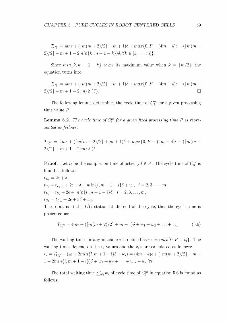
CHAPTER 5. PURE CYCLES IN ROBOT CENTERED CELLS 59
TCm2
= 4mε + (dm(m + 2)/2e+ m + 1)δ + max{0, P − (4m− 4)ε− (dm(m +
2)/2e+ m + 1− 2min{k, m + 1− k})δ;∀k ∈ [1, . . . , m]}.
Since min{k,m + 1 − k} takes its maximum value when k = dm/2e, the
equation turns into:
TCm2
= 4mε + (dm(m + 2)/2e+ m + 1)δ + max{0, P − (4m− 4)ε− (dm(m +
2)/2e+ m + 1− 2dm/2e)δ}.
The following lemma determines the cycle time of Cm3 for a given processing
time value P .
Lemma 5.2. The cycle time of Cm3 for a given fixed processing time P is repre-
sented as follows:
TCm3
= 4mε + (dm(m + 2)/2e + m + 1)δ + max{0, P − (4m − 4)ε − (dm(m +
2)/2e+ m + 1− 2dm/2e)δ}.
Proof. Let tl be the completion time of activity l ∈ A. The cycle time of Cm3 is
found as follows:
tL1 = 2ε + δ,
tUi= tLi−1
+ 2ε + δ + min{i,m + 1− i}δ + wi, i = 2, 3, . . . , m,
tLi= tUi
+ 2ε + min{i,m + 1− i}δ, i = 2, 3, . . . , m,
tU1 = tLm + 2ε + 3δ + w1.
The robot is at the I/O station at the end of the cycle, thus the cycle time is
presented as:
TCm3
= 4mε + (dm(m + 2)/2e+ m + 1)δ + w1 + w2 + . . . + wm (5.6)
The waiting time for any machine i is defined as wi = max{0, P − vi}. The
waiting times depend on the vi values and the vi’s are calculated as follows:
vi = TCm3− (4ε + 2min{i,m + 1− i}δ + wi) = (4m− 4)ε + (dm(m + 2)/2e+ m +
1− 2min{i,m + 1− i})δ + w1 + w2 + . . . + wm − wi,∀i.
The total waiting time∑
∀i wi of cycle time of Cm3 in equation 5.6 is found as
follows:

CHAPTER 5. PURE CYCLES IN ROBOT CENTERED CELLS 60
1. If P ≤ vi,∀i then, w1 + w2 + . . . + wm = 0
2. Else if ∃k ∈ [1, . . . , m] such that vk < P , then wk = P − vk = P − (4m−4)ε − (dm(m + 2)e + m + 1 − 2min{k,m + 1 − k})δ − ∑
i 6=k wi. Hence,
w1 +w2 + . . .+wm = P − (4m−4)ε− (dm(m+2)/2e+m+1−2min{k, m+
1− k})δ.
Now we can state that:
TCm3
= 4mε + (dm(m + 2)/2e+ m + 1)δ + max{0, P − (4m− 4)ε− (dm(m +
2)/2e+ m + 1− 2min{k, m + 1− k})δ;∀k ∈ [1, . . . , m]}.
Since min{k,m + 1 − k} takes its maximum value when k = dm/2e, the
equation turns into:
TCm3
= 4mε + (dm(m + 2)/2e+ m + 1)δ + max{0, P − (4m− 4)ε− (dm(m +
2)/2e+ m + 1− 2dm/2e)δ}.
In the next theorem, the cycle time lower bound of pure cycles for the robot
centered cells with I/O station is determined.
Theorem 5.1. For an m-machine robot centered cell, the cycle time of any pure
cycle is no less than
TI/O = max{4mε + dm(m + 2)/2eδ, 4ε + 2dm/2eδ + P}. (5.7)
Proof. A lower bound for a pure cycle can be calculated by using two different
definitions of the cycle time. The first lower bound is obtained from the exact
robot activity time and the second is obtained from the given processing time
vector. Since the robot has to perform an exact set of robot activities, the total
time required for these activities constitutes a lower bound. Thus, the first lower
bound is obtained as follows: The set of robot activities can be analyzed in two
groups and the first group is robot loading and unloading times. First, a part is
taken from the I/O station (ε), then loaded to one of the machines (ε), after the
processing on the machine is finished, the part is unloaded (ε) and dropped to the
I/O station (ε). This makes a total of 4mε for a repetition of cycle. The robot

CHAPTER 5. PURE CYCLES IN ROBOT CENTERED CELLS 61
travel times constitute the second group of robot activities. The robot takes a
part from I/O station and travels to machine i to load it (min{i,m + 1 − i}δ),after the processing on the part is finished, robot unloads the machine and travels
to the I/O station to drop the finished part (min{i,m + 1− i}δ).
1. Suppose the number of machines is even, then the total robot travel time
is calculated as:∑mi=1 min{i,m + 1− i}δ = 2δ + 4δ + 6δ + . . . + mδ + mδ + (m− 2)δ + (m−
4)δ + . . . + 2δ = dm(m + 2)/2eδ.
2. Suppose the number of machines is odd, then the total robot travel time is
calculated as:∑mi=1 min{i,m + 1− i}δ = 2δ + 4δ + 6δ + . . . + (m + 1)δ + (m− 1)δ + (m−
3)δ + . . . + 2δ = dm(m + 2)/2eδ.
Consequently, the total of robot activities require at least 4mε + dm(m + 2)/2eδtime units.
The second definition of a cycle time that leads to another lower bound is the
minimum time between two consecutive loadings of any machine. The minimum
time needed to unload machine i after loading it is P time units. After processing
of the part is finished, the part is unloaded (ε), it is transferred to I/O station
(min{i,m + 1− i}δ), and dropped (ε). After that, the robot takes a new part to
make the consecutive loading of machine i (ε), brings the new part to machine i
(min{i,m+1−i}δ) and finally loads the machine (ε). The total time between two
consecutive loadings of machine i is at least 4ε+2min{i,m+1−i}δ+P . However
there are m machines and the total time for consecutive loadings are different for
each of them. Thus, the cycle time has to be greater than or equal to the minimum
time required between two consecutive loadings of any machine in the cell. So,
the second lower bound of the cycle time is 4ε + 2max{min{i,m + 1 − i}, i :
1, . . . , m}δ + P .
As can be seen from Lemma 5.1 and Lemma 5.2, the pure cycles Cm2 and Cm
3
result in the same cycle time for each processing time. Thus, the processing time

CHAPTER 5. PURE CYCLES IN ROBOT CENTERED CELLS 62
region where they result in the minimum cycle time for pure cycles will be the
same as well. The next theorem determines the processing time region where
either Cm2 or Cm
3 dominates the rest of pure cycles.
Theorem 5.2. For an m-machine robot centered cell, either Cm2 or Cm
3 dominates
the rest of pure cycles in the processing time region:
(4m− 4)ε + (dm(m + 2)/2e+ m + 1− 2dm/2e)δ ≤ P
Proof. If (4m− 4)ε + (dm(m + 2)/2e+ m + 1− 2dm/2e)δ ≤ P , then
TCm2
= TCm3
= 4ε + 2dm/2eδ + P = TI/O.
Figure 5.2: Cycle time-Processing time region where Cm2 dominates the rest of
pure cycles
In Figure 5.2, we can see the processing time region where either Cm2 or Cm
3
dominates the rest of pure cycles and the corresponding cycle time region. From
Theorem 5.2, for the processing time region 0 < P < (4m − 4)ε + (dm(m +
2)/2e + m + 1 − 2dm/2e)δ, Cm2 does not dominate the rest of pure cycles. For
the processing time region (4m− 4)ε + (dm(m + 2)/2e+ m + 1− 2dm/2e)δ ≤ P ,
either Cm2 or Cm
3 results in the cycle time lower bound. This processing time
region corresponds to the cycle time region 4mε+(dm(m+2)/2e+m+1)δ ≤ K.
Consequently, it is observed that the only cycle time region where Cm2 and Cm
3
is not optimum is the only region starting from cycle time lower bound and the
size of this region is (m + 1)δ time units. This region becomes smaller relative to
whole cycle time region as the number of machines increases.

CHAPTER 5. PURE CYCLES IN ROBOT CENTERED CELLS 63
In the next lemma, for the remaining processing time region where neither Cm2
nor Cm3 does not result in minimum cycle time the worst case performances of the
two cycles are calculated. The worst case performance is calculated by comparing
cycle time are obtained from Cm2 and Cm
3 to the cycle time lower bound in the
mentioned processing time region. Since Cm2 and Cm
3 result in the same cycle
time for any processing time, their worst case performances are equal. Let T ∗
represents the minimum cycle time obtained from pure cycles in the described
processing time region.
Lemma 5.3. For the remaining processing time region:
P < (4m− 4)ε + (dm(m + 2)/2e+ m + 1− 2dm/2e)δ
the performance of either Cm2 or Cm
3 in this region is stated as:
TCm2
, TCm3≤ (1 +
(m + 1)δ
4mε + dm(m + 2)/2eδ ) · T ∗.
Proof. The cycle time of Cm2 and Cm
3 are equal TCm2
= TCm3
as can be seen
from equation of TCm2
in Lemma 5.1 and equation of TCm3
in Lemma 5.2 . In the
mentioned processing time region, the lower bound of cycle time is calculated
from Theorem 5.1 as 4mε + dm(m + 2)/2eδ ≤ TI/O. Then,
TCm3
T ∗ =TCm
2
T ∗ ≤ TCm2
TI/O≤ 4mε+(dm(m+2)/2e+m+1)δ
4mε+dm(m+2)/2eδ = 1 + (m+1)δ4mε+dm(m+2)/2eδ .
The only region where neither Cm2 nor Cm
3 does not dominate the rest of
pure cycles is the processing time region P < (4m − 4)ε + (dm(m + 2)/2e +
m + 1− 2dm/2e)δ. The difference between cycle time lower bound and the cycle
time of either Cm2 or Cm
3 in this region decreases as the number of machines
increases and vice versa. In order to see the decrease in difference between cycle
time lower bound and cycle time of either Cm2 or Cm
3 as the number of machines
increases, the 2-machine cell and m-machine cell where m → ∞ are analyzed
for this processing time region. Firstly, the maximum difference between lower
bound and cycle time of either Cm2 or Cm
3 is observed in 2-machine cell. The cycle
time lower bound is calculated from Theorem 5.1 as 8ε + 4δ ≤ TI/O. The cycle
time of either C22 or C2
3 is determined from Lemma 5.1 as TC23
= TC22
= 8ε + 7δ.

CHAPTER 5. PURE CYCLES IN ROBOT CENTERED CELLS 64
The difference between either TCm2
or TCm3
and the lowest cycle time that can be
obtained from pure cycles T ∗ is determined by using Lemma 5.3 as TC23
= TC22≤
(1 + (m+1)δ4mε+dm(m+2)/2eδ ) · T ∗ = (1 + 3δ
8ε+4δ) · T ∗. Hence, the worst case of difference
between either TC22
or TC23
and T ∗ is 3δ8ε+4δ
· T ∗. The difference between TCm2
, TCm3
and T ∗ takes its minimum value as m →∞ and it is determined by using Lemma
5.3 as TCm3
= TCm2≤ (1 + (m+1)δ
4mε+dm(m+2)/2eδ ) · T ∗ = T ∗. Since, cycle time of either
Cm2 or Cm
3 is at least equal to T ∗ ≤ TCm2
= TCm3
, the cycle time obtained from
either Cm2 or Cm
3 is equal to the minimum cycle time, TCm3
= TCm2
= T ∗. Thus,
we say that the difference between either TCm2
or TCm3
and T ∗ decreases as the
number of machines increases.
5.1.3 3-Machine Analysis
In the Figure 5.3, the pure cycles resulting in minimum cycle time for pure cycles
are presented among all possible 3-machine cell. There are 120 pure cycles in a
3-machine cell and we have calculated the cycle times of all of these pure cycles.
However, they cannot be presented in the graph because of space limitation, only
12 of the pure cycles are presented. The cycle time of these pure cycles are pre-
sented as follows:
C31 = L1L3U2L2U1U3 with cycle time TC3
1= 12ε + 12δ + max{0, P − 8δ − 6ε},
C32 = L1U3L3U2L2U1 with cycle time TC3
2= 12ε + 12δ + max{0, P − 8δ − 8ε},
C33 = L1U2L2U3L3U1 with cycle time TC3
3= 12ε + 12δ + max{0, P − 8δ − 8ε},
C34 = L1U1L2U2L3U3 with cycle time TC3
4= 12ε + 8δ + 3P ,
C35 = L1U1L2U2U3L3 with cycle time TC3
5= 12ε + 10δ + 2P ,
C36 = L1U1L2L3U2U3 with cycle time TC3
6= 12ε+12δ +P +max{0, P − 4δ−2ε},
C37 = L1U2L2U1L3U3 with cycle time TC3
7= 12ε+10δ +P +max{0, P − 6δ−4ε},
C38 = L1L2L3U1U2U3 with cycle time TC3
8= 12ε + 16δ + max{0, P − 8δ − 4ε}.
In addition the robot move sequences and cycle times of pure cycles C311, C3
12, C315
and C319 are presented in Table 5.1.
The cycle time lower bound is found by using Theorem 5.1 as:
TI/O = max{12ε + 8δ, 4ε + 4δ + P}.

CHAPTER 5. PURE CYCLES IN ROBOT CENTERED CELLS 65
12 12ε + δ
3 3
4 19,C C
3
5C3
6C3 3 3 3
7 11 12 15, , ,C C C C
3 3
2 3,C C
3
1C
3
8C
Processing time
Cycle time
12 8ε + δ
12 11ε + δ
88ε + δ δ 2δ
/I OT
Figure 5.3: 3-machine cell analysis
The graph in Figure 5.3 is useful in order to see the efficiency of C32 and C3
3 in
a 3-machine cell. The dashed line in the graph (TI/O) represents the cycle time
lower bound found by using Theorem 5.1. The bold lines in the graph represents
the minimum cycle time corresponding to processing times. Either C32 or C3
3
results in the minimum cycle time in the processing time region 2δ ≤ P . The
only region where neither C32 nor C3
3 does not dominate the rest is the region of
P < 2δ. Consequently, the efficiency of cycles C32 and C3
3 in order to minimize
cycle time is presented in 3-machine cells.
In the next theorem, the pure cycles minimizing cycle time and corresponding
processing time regions are presented for 3-machine cells.
Theorem 5.3. For 3-machine case
1. If P < δ, then either C34 or C3
19 results in minimum cycle time for pure
cycles,
2. If δ ≤ P < 2δ, then either C37 or C3
11 or C312 or C3
15 results in minimum
cycle time for pure cycles,
3. If P ≥ 2δ, then either C32 or C3
3 results in minimum cycle time for pure

CHAPTER 5. PURE CYCLES IN ROBOT CENTERED CELLS 66
cycles.
Proof. There are 120 different pure cycles and we calculated the cycle time
of all these pure cycles. The proof consists of 4 parts and in order to obtain these
results, the cycle time of 120 pure cycles are compared with the proposed cycles.
1. When K < 12ε+10δ, only C34 and C3
19 are feasible pure cycles in this region
and they result in the same cycle time as can be seen in Table 5.1. The
corresponding processing time region for this cycle time region is P < 2δ/3.
Thus, there is no other pure cycle that can result in less cycle time than
either C34 or C3
19.
2. When 12ε + 10δ ≤ K < 12ε + 12δ, all of the 14 pure cycles presented in
Table 5.1 are feasible. When we compare the cycle time of C34 and C3
19 with
the other 12 pure cycles, either C34 or C3
19 results in the minimum cycle time
in the processing time region 2δ/3 ≤ P < δ which corresponds to the cycle
time region 12ε+10δ ≤ K < 12ε+11δ. The cycle times of C37 , C3
11, C312 and
C315 are equal for any processing time as can be seen in Table 5.1. Similarly
by comparing the cycle time of C37 , C3
11, C312 and C3
15 with the cycle time of
other 10 feasible pure cycles, the cycle time of C37 , C3
11, C312 and C3
15 is the
minimum cycle time for processing time region δ ≤ P < 2δ corresponding
to cycle time region 12ε + 11δ ≤ K < 12ε + 12δ.
3. There are 24 feasible pure cycles at cycle time K = 12ε+12δ when 2δ ≤ P .
When we compare cycle time of either C32 or C3
3 with the rest of pure
cycles, the cycle time of either C32 or C3
3 is the minimum cycle time for the
processing time region 2δ ≤ P < 8ε + 8δ.
4. From Theorem 4.2, either C32 or C3
3 results in the minimum cycle time for
the processing time region 8ε + 8δ ≤ P .
Table 5.1 presents the robot move sequences and total cycle time for 14 pure
cycles which are used in the proof of Theorem 5.3.

CHAPTER 5. PURE CYCLES IN ROBOT CENTERED CELLS 67
Cycle Robot move sequence Cycle Time (TC3i)
C34 L1U1L2U2L3U3 12ε + 8δ + 3P
C35 L1U1L2U2U3L3 12ε + 10δ + 2P
C37 L1U2L2U1L3U3 12ε + 10δ + P + max{0, P − 4ε− 6δ}
C39 L1L3U3L2U2U1 12ε + 10δ + 2P
C310 L1L3U3U1L2U2 12ε + 10δ + 2P
C311 L1U2L3U3L2U1 12ε + 10δ + P + max{0, P − 4ε− 4δ}
C312 L1U1L2U3L3U2 12ε + 10δ + P + max{0, P − 4ε− 4δ}
C313 L1L2U2L3U3U1 12ε + 10δ + 2P
C314 L1L2U2U1L3U3 12ε + 10δ + 2P
C315 L1U1L3U2L2U3 12ε + 10δ + P + max{0, P − 4ε− 6δ}
C316 L1U1L3L2U2U3 12ε + 10δ + 2P
C317 L1U1U3L2U2L3 12ε + 10δ + 2P
C318 L1U1U3L3L2U2 12ε + 10δ + 2P
C319 L1U1L3U3L2U2 12ε + 8δ + 3P
Table 5.1: Some of the robot move sequences and corresponding cycle times in3-machine robotic cells
5.1.4 Discussion
In this section, we analyzed the pure cycles in robot centered cells where the ma-
chines are CNC machines. The processing times are assumed to be fixed and the
same on every machine. The problem was to determine the robot move sequences
minimizing cycle time for a given processing time. Consequently, it is proved that
either Cm2 or Cm
3 results in the minimum cycle time for the specified processing
time region in Theorem 5.2. For the remaining region where neither Cm2 nor Cm
3
does not result in minimum cycle time, the worst case performance analysis made
by comparing the cycle time of Cm2 and Cm
3 to cycle time lower bound in that
processing time region. In addition, the cycles resulting in minimum cycle time
in 3-machine robot centered cell are determined. In 3-machine cell analysis, it is
observed that either Cm2 or Cm
3 results in the minimum cycle time for most of the
processing time region.
Until now, we have focused on the cycle time objective and we find that
either C32 or C3
3 results in minimum cycle time for a specified processing time
region. From now on, the controllability is introduced to our problem so that the

CHAPTER 5. PURE CYCLES IN ROBOT CENTERED CELLS 68
processing times can be increased or decreased. The efficient cycles that minimize
both cycle time and total manufacturing cost simultaneously are investigated.
Since Cm2 and Cm
3 minimize cycle time in most of the processing time region, we
propose that Cm2 and Cm
3 are efficient pure cycles for this bicriteria problem. In
the next section, the cycle time region where either Cm2 or Cm
3 dominates the rest
is determined.
5.2 Bicriteria Analysis of Cm2 and Cm
3
In this part, there is an m-machine robot centered cell and the processing times
are assumed to be controllable. The objective is the bicriteria objective of mini-
mizing cycle time and total manufacturing cost simultaneously. The pure cycles
Cm2 and Cm
3 are proved to result in minimum cycle time in a specified processing
time region in the previous chapter. Thus, we propose that these two prominent
cycles are effective pure cycles in terms of these two objectives. For the stated
bicriteria optimization problem, the 3-machine case analysis according to this bi-
criteria objective is presented. In 3-machine robot centered cell, the pure cycles
and processing time vectors resulting in both minimum cycle time and minimum
total manufacturing cost for specified cycle time regions are determined.
5.2.1 Problem Definition
In this section, different from the previous section, the machines are considered
as highly flexible CNC machines in which the processing times are controllable
such that it enables us to increase or decrease the processing times. The feasible
processing times on machines are assumed to be between a lower bound and an
upper bound which is denoted by PL ≤ Pi ≤ PU . A processing time vector is
denoted as P = (P1, P2, . . . , Pm). Feasible processing time vectors are composed
of feasible processing times and the set of feasible processing time vectors is
denoted as Pfeas = {(P1, P2, . . . , Pm) ∈ Rm : PL ≤ Pi ≤ PU , ∀i}.

CHAPTER 5. PURE CYCLES IN ROBOT CENTERED CELLS 69
5.2.2 Solution Procedure
In this part, we present the solution method for this problem. First, we find the
cycle time of proposed pure cycles Cm2 and Cm
3 when a processing time vector is
given. Afterwards, we find the processing time vector resulting in lower bound of
total manufacturing cost for pure cycles. The nondominated solutions of Cm2 and
Cm3 are determined. The total manufacturing cost obtained from nondominated
solutions of Cm2 and Cm
3 are compared with the lower bound of total manufactur-
ing cost. By this way, the cycle time region where either Cm2 or Cm
3 dominates
the rest of pure cycles is determined. The next lemma determines the cycle time
of either Cm2 or Cm
3 when there is a given processing time vector.
Lemma 5.4. The cycle time of either Cm2 or Cm
3 for a given processing time
vector is presented as follows:
TCm2
= TCm3
= 4mε + (dm(m + 2)/2e + m + 1)δ + max{0,max{Pi − (4m −4)ε− (dm(m + 2)e+ m + 1− 2min{i, m + 1− i})δ, i : 1, . . . , m}}.
Proof. The cycle time of Cm2 in equation (5.5) and the cycle time of Cm
3 in
equation (5.6) are the same and defined as follows:
4mε + (dm(m + 2)/2e+ m + 1)δ + w1 + w2 + . . . + wm.
So, we can see that robot load/unload times and robot travel times are the same
in TCm2
and in TCm3
. The waiting times are the same in TCm2
and in TCm3
and
defined as wi = max{0, Pi− vi} where vi = (4m− 4)ε+(dm(m+2)/2e+m+1−2min{i,m + 1 − i})δ + w1 + w2 + . . . + wm − wi for all machines. So, the cycle
time of Cm2 and Cm
3 are equal for any processing time.
There are two different total waiting time results and the sufficient conditions
for these cases are determined as follows:
1. If Pi ≤ vi for ∀i ∈ [1, . . . , m], then wi = 0, for i = 1, . . . , m
2. Else if ∃k ∈ [1, . . . , m] such that vk < Pk , then wk = Pk − vk = Pk −(4m−4)ε− (dm(m+2)e+m+1−2min{k, m+1−k})δ−∑
i6=k wi. Hence,

CHAPTER 5. PURE CYCLES IN ROBOT CENTERED CELLS 70
w1 +w2 + . . .+wm = Pk−(4m−4)ε−(dm(m+2)/2e+m+1−2min{k, m+
1− k})δ.
So, w1 + w2 + . . . + wm = max{0,max{Pk − (4m− 4)ε− (dm(m + 2)e+ m + 1−2min{k, m + 1 − k})δ} and the cycle time is obtained by replacing the total of
waiting time in equations (5.5) and (5.6) with this max function.
In the next theorem, the cycle time lower bound for pure cycles in robot
centered cells is determined when a processing time vector is given.
Theorem 5.4. For an m-machine robot centered cell with controllable processing
times, the cycle time of any pure cycle is no less than:
TI/0,contr = max{4mε+dm(m+2)/2eδ, 4ε+2max{min{i,m+1−i}δ+Pi, i : 1, . . . , m}}.(5.8)
Proof. From the definition of pure cycles, we determined that the cycle time of
a pure cycle has to be at least equal to two lower bounds. The first lower bound
is obtained from the exact robot activity time and the second one is obtained
from the given processing time vector. Since the robot has to perform an exact
set of robot activities, the total time required for these activities constitutes a
lower bound. Thus, the first lower bound is obtained as follows: The set of robot
activities can be analyzed in two groups and the first group is robot loading and
unloading times. First, a part is taken from the I/O station (ε), then loaded
to one of the machines (ε), after the processing on the machine is finished, the
part is unloaded (ε) and dropped to the I/O station (ε). This makes a total
of 4mε for a repetition of cycle. The robot travel times constitute the second
group of robot activities. The robot takes a part from I/O station and travels to
machine to load it (min{i, m+1−i}δ), after the processing on the part is finished,
robot unloads machine and travels to the I/O station to drop the finished part
(min{i,m + 1− i}δ).
1. Suppose the number of machines is even, then the total robot travel time
is calculated as:
CHAPTER 5. PURE CYCLES IN ROBOT CENTERED CELLS 71
∑mi=1 min{i,m + 1− i}δ = 2δ + 4δ + 6δ + . . . + mδ + mδ + (m− 2)δ + (m−
4)δ + . . . + 2δ = dm(m + 2)/2eδ.
2. Suppose the number of machines is odd, then the total robot travel time is
calculated as:∑mi=1 min{i,m + 1− i}δ = 2δ + 4δ + 6δ + . . . + (m + 1)δ + (m− 1)δ + (m−
3)δ + . . . + 2δ = dm(m + 2)/2eδ.
Consequently, the total of robot activities require at least 4mε + dm(m + 2)/2eδtime units.
The second lower bound is the minimum time required between two consec-
utive loadings of any machine. The minimum time needed to unload machine i
after loading it is Pi time units. After the processing on the part is finished, it is
unloaded (ε), transferred to the I/O station (min{i,m + 1 − i}δ), and dropped
(ε). After that, the robot takes a new part to make the consecutive loading of
machine i (ε), brings the new part to machine i (min{i,m + 1− i}δ) and finally
loads the machine (ε). The total time between two consecutive loadings of ma-
chine i is at least 4ε+2min{i,m+1−i}δ+Pi. However there are m machines and
the total time for consecutive loadings are different from each other. Thus, the
cycle time has to be greater than or equal to the minimum time required between
two consecutive loadings of any machine in the cell. So, the second lower bound
of the cycle time is 4ε + max{2min{i,m + 1− i}δ + Pi}, ∀i.
In the next lemma, the upper bound of processing time vectors of pure cycles
for a given cycle time level K is determined.
Lemma 5.5. For a given cycle time level K, the upper bound of processing time
vectors in robot centered cells for pure cycles is represented as follows:
P(K) = (P 1(K), . . . , Pm(K)),
where P i(K) = min{PU , K − (4ε + 2min{i,m + 1− i}δ)}, ∀i.
Proof. The two bounds constraining processing time vectors are found in the
following cases.

CHAPTER 5. PURE CYCLES IN ROBOT CENTERED CELLS 72
1. The processing times are less than PU which leads to P i(K) ≤ PU , ∀i.
2. In addition, the processing times on machines cannot exceed a specific value,
since the cycle time is bounded by K. The cycle time level K constrains
the processing times. Now, we find the upper bound of processing time on
machine i, Pi, for the cycle time level K. The cycle time lower bound is
determined by using equation (5.8) in Theorem 5.4 which is presented as:
TI/0,contr = max{4mε+dm(m+2)/2eδ, 4ε+max{2min{i,m+1−i}δ+Pi, i :
1, . . . , m}}.Let us set the cycle time K, then cycle time is at least equal to the cycle
time lower bound :
TI/0,contr = max{4mε+dm(m+2)/2eδ, 4ε+max{2min{i,m+1−i}δ+Pi, i :
1, . . . , m}} ≤ K
Now, the processing time upper bound for machine i is found as follows:
max{2min{i,m + 1− i}δ + Pi, i : 1, . . . , m} ≤ K − 4ε, then Pi ≤ K − 4ε−2min{i,m + 1− i}δ, ∀i. This implies that:
P i(K) ≤ K − (4ε + 2min{i, m + 1− i}δ),∀i.
Hence, the P(K) is upper bound of processing time vectors satisfying the two
bounds described above for a given cycle time level.
The cycle times of Cm2 and Cm
3 are equal for any processing time vector as
defined in Lemma 5.4. Since the set of nondominated points is calculated only
according to cycle time definition as presented in the proof of Lemma 5.6 and
the cycle time of Cm2 and Cm
3 are the same, Cm2 and Cm
3 result in the same set
of nondominated processing time vectors, P∗(Cm2 |K) = P∗(Cm
3 |K). In the next
lemma, the processing time vector that gives the minimum total manufacturing
cost obtained from either Cm2 or Cm
3 for a given cycle time level K is determined.
Lemma 5.6. Given any feasible cycle time level K, the nondominated processing
time vector of either Cm2 or Cm
3 is defined as (P ∗1 , P ∗
2 , . . . , P ∗m) ∈ (P∗(Cm
2 |K) =
P∗(Cm3 |K)) where P ∗
i = min{PU , K − (4ε + 2min{i,m + 1− i}δ)},∀i.

CHAPTER 5. PURE CYCLES IN ROBOT CENTERED CELLS 73
Proof. For a given cycle time level K, a feasible processing time vector is com-
posed of processing times on machines that satisfy two upper bounds.
1. All processing times are less than PU which leads to P ∗i ≤ PU ,∀i.
2. In addition, the processing times are bounded such that not to violate the
cycle time level K. The processing time on machine i, Pi, is constrained
according to the cycle time K. By using Lemma 5.4 and fixing cycle time
to K, the cycle time can be presented as follows:
K = 4mε + (dm(m + 2)/2e + m + 1)δ + max{0,max{Pi − (4m − 4)ε −(dm(m + 2)e+ m + 1− 2min{i,m + 1− i})δ, i : 1, . . . , m}}This leads to Pi ≤ K − (4ε + 2min{i, m + 1 − i}δ). Since P ∗
i is feasible,
P ∗i ≤ K − (4ε + 2min{i,m + 1− i}δ),∀i.
The processing times on their maximum values, without violating the bounds
found in the first and second arguments, compose the nondominated processing
time vectors in Lemma 5.6.
In the next example, the nondominated processing time vector of Cm2 and Cm
3
for a given cycle time level is determined as defined in Lemma 5.6.
Example 5.1 There is a 5-machine robot centered cell. Let δ = 0.1, ε = 0.1,
PL = 3.0, PU = 4.5 and K = 5.0. For this cycle time level, the nondominated
processing time vector (P ∗1 , P ∗
2 , P ∗3 , P ∗
4 , P ∗5 ) ∈ (P∗(C5
2 |5.0) = P∗(C53 |5.0)) is calcu-
lated by using Lemma 5.6 as follows:
P∗(C52 |5.0) = P∗(C5
3 |5.0) =
P ∗1
P ∗2
P ∗3
P ∗4
P ∗5
=
min{PU , K − (4ε + 2δ)}min{PU , K − (4ε + 4δ)}min{PU , K − (4ε + 6δ)}min{PU , K − (4ε + 4δ)}min{PU , K − (4ε + 2δ)}
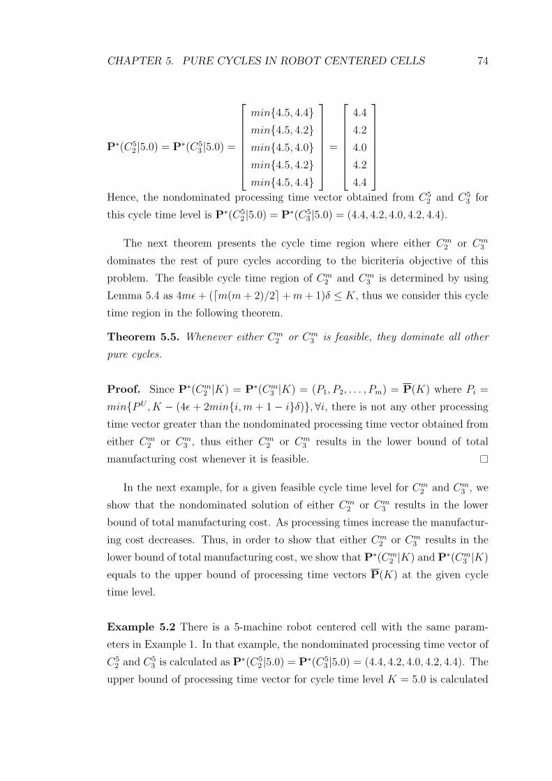
CHAPTER 5. PURE CYCLES IN ROBOT CENTERED CELLS 74
P∗(C52 |5.0) = P∗(C5
3 |5.0) =
min{4.5, 4.4}min{4.5, 4.2}min{4.5, 4.0}min{4.5, 4.2}min{4.5, 4.4}
=
4.4
4.2
4.0
4.2
4.4
Hence, the nondominated processing time vector obtained from C52 and C5
3 for
this cycle time level is P∗(C52 |5.0) = P∗(C5
3 |5.0) = (4.4, 4.2, 4.0, 4.2, 4.4).
The next theorem presents the cycle time region where either Cm2 or Cm
3
dominates the rest of pure cycles according to the bicriteria objective of this
problem. The feasible cycle time region of Cm2 and Cm
3 is determined by using
Lemma 5.4 as 4mε + (dm(m + 2)/2e+ m + 1)δ ≤ K, thus we consider this cycle
time region in the following theorem.
Theorem 5.5. Whenever either Cm2 or Cm
3 is feasible, they dominate all other
pure cycles.
Proof. Since P∗(Cm2 |K) = P∗(Cm
3 |K) = (P1, P2, . . . , Pm) = P(K) where Pi =
min{PU , K − (4ε + 2min{i,m + 1 − i}δ)}, ∀i, there is not any other processing
time vector greater than the nondominated processing time vector obtained from
either Cm2 or Cm
3 , thus either Cm2 or Cm
3 results in the lower bound of total
manufacturing cost whenever it is feasible.
In the next example, for a given feasible cycle time level for Cm2 and Cm
3 , we
show that the nondominated solution of either Cm2 or Cm
3 results in the lower
bound of total manufacturing cost. As processing times increase the manufactur-
ing cost decreases. Thus, in order to show that either Cm2 or Cm
3 results in the
lower bound of total manufacturing cost, we show that P∗(Cm2 |K) and P∗(Cm
3 |K)
equals to the upper bound of processing time vectors P(K) at the given cycle
time level.
Example 5.2 There is a 5-machine robot centered cell with the same param-
eters in Example 1. In that example, the nondominated processing time vector of
C52 and C5
3 is calculated as P∗(C52 |5.0) = P∗(C5
3 |5.0) = (4.4, 4.2, 4.0, 4.2, 4.4). The
upper bound of processing time vector for cycle time level K = 5.0 is calculated

CHAPTER 5. PURE CYCLES IN ROBOT CENTERED CELLS 75
from Lemma 5.5 as follows:
P(K) =
P 1(K)
P 2(K)
P 3(K)
P 4(K)
P 5(K)
=
min{PU , K − (4ε + 2δ)}min{PU , K − (4ε + 4δ)}min{PU , K − (4ε + 6δ)}min{PU , K − (4ε + 4δ)}min{PU , K − (4ε + 2δ)}
=
min{4.5, 4.4}min{4.5, 4.2}min{4.5, 4.0}min{4.5, 4.2}min{4.5, 4.4}
This simply implies that:
P(K) =
4.4
4.2
4.0
4.2
4.4
Hence, the upper bound of processing time vectors is found as P(K) =
(4.4, 4.2, 4.0, 4.2, 4.4). Since the nondominated processing time vector of C52
and C53 are equal to the upper bound of processing time vectors P∗(C5
2 |5.0) =
P∗(C53 |5.0) = P(K), there is no other pure cycle that can result in less total
manufacturing cost than either C52 or C5
3 .
5.2.3 3-Machine Case with Controllable Processing Times
In Figure 5.4, the efficient frontier of 3-machine problem is presented. The bold
lines in the figure represent the efficient frontier such that the minimum total
manufacturing cost obtained at the corresponding cycle time. The cycle time
lower bound of pure cycles in 3-machine cell is calculated by using Theorem
5.4 as 12ε + 8δ. Either C34 or C3
19 dominates the rest in the cycle time region
12ε + 8δ ≤ K < K1. K1 is always between 12ε + 10δ < K1 < 12ε + 12δ and the
exact value of K1 differs according to the manufacturing cost function f . At the
cycle time value of K1, the total manufacturing cost of P∗(C34 |K1), P∗(C3
19|K1),
P∗(C37 |K1) and P∗(C3
15|K1) are equal. After that, either C37 or C3
15 results in the
minimum cycle time for the cycle time region K1 < K < 12ε + 12δ. The pure
cycles C32 and C3
3 are feasible in the region 12ε+12δ ≤ K and from Theorem 5.5,

CHAPTER 5. PURE CYCLES IN ROBOT CENTERED CELLS 76
either C32 or C3
3 dominates the rest in this region. The cycle times corresponding
to the 14 feasible pure cycles when K < 12ε + 12δ are presented as follows:
TC34
= TC319
= 12ε + 8δ + P1 + P2 + P3
TC35
= TC318
= 12ε + 10δ + P1 + P2 + max{0, P3 − 8ε− 8δ − P1 − P2}TC3
7= 12ε+10δ+max{0, P1−4ε−6δ−w2}+max{0, P2−8ε−6δ−w1−P3}+P3
TC39
= TC313
= 12ε + 10δ + max{0, P1 − 8ε− 8δ − P3 − P2}+ P2 + P3
TC310
= 12ε + 10δ + max{0, P1 − 4ε− 4δ − P3}+ P2 + P3
TC311
= 12ε+10δ+max{0, P1−8ε−8δ−P3−w2}+max{0, P2−4ε−4δ−w1}+P3
TC312
= 12ε+10δ+P1 +max{0, P2−4ε−4δ−w3}+max{0, P3−8ε−8δ−w2−P1}TC3
14= 12ε + 10δ + max{0, P1 − 4ε− 6δ − P2}+ P2 + P3
TC315
= 12ε+10δ+P1 +max{0, P2−8ε−6δ−P1−w3}+max{0, P3−4ε−6δ−w2}TC3
16= 12ε + 10δ + P1 + P2 + max{0, P3 − 4ε− 6δ − P2}
TC317
= 12ε + 10δ + P1 + P2 + max{0, P3 − 4ε− 4δ − P1}
Cycle Robot move sequenceC3
4 L1U1L2U2L3U3
C35 L1U1L2U2U3L3
C37 L1U2L2U1L3U3
C39 L1L3U3L2U2U1
C310 L1L3U3U1L2U2
C311 L1U2L3U3L2U1
C312 L1U1L2U3L3U2
C313 L1L2U2L3U3U1
C314 L1L2U2U1L3U3
C315 L1U1L3U2L2U3
C316 L1U1L3L2U2U3
C317 L1U1U3L2U2L3
C318 L1U1U3L3L2U2
C319 L1U1L3U3L2U2
Table 5.2: The feasible pure cycles in the cycle time region K < 12ε + 12δ andcorresponding robot move sequences

CHAPTER 5. PURE CYCLES IN ROBOT CENTERED CELLS 77
Cycle P∗(C3i |K)
Machine 1 Machine 2 Machine 3C3
4 (K − 12ε− 8δ)/3 (K − 12ε− 8δ)/3 (K − 12ε− 8δ)/3C3
5 (K − 12ε− 10δ)/2 (K − 12ε− 10δ)/2 K − 4ε− 2δC3
7 4ε + 6δ K − 4ε− 4δ K − 12ε− 10δC3
9 K − 4ε− 2δ (K − 12ε− 10δ)/2 (K − 12ε− 10δ)/2C3
10 a1 a2 a3
C311 K − 4ε− 2δ 4ε + 4δ K − 12ε− 10δ
C312 K − 12ε− 10δ 4ε + 4δ K − 4ε− 2δ
C313 K − 4ε− 2δ (K − 12ε− 10δ)/2 (K − 12ε− 10δ)/2
C314 (K − 4ε + 2δ)/2 (K − 12ε− 10δ)/2 (K − 12ε− 10δ)/2
C315 K − 12ε− 10δ K − 4ε− 4δ 4ε + 6δ
C316 b1 b2 b3
C317 c1 c2 c3
C318 (K − 12ε− 10δ)/2 (K − 12ε− 10δ)/2 K − 4ε− 2δ
C319 (K − 12ε− 8δ)/3 (K − 12ε− 8δ)/3 (K − 12ε− 8δ)/3
Table 5.3: The processing times of optimum solutions of feasible pure cycles inthe cycle time region K < 12ε + 12δ
The values of aj, bj and cj for j = 1, 2, 3 in Table 5.3 are presented as follows:
a1 ≤ K − 8ε− 6δ, a2 ≤ K − 12ε− 10δ, a3 ≤ K − 12ε− 10δ,
b1 ≤ K − 12ε− 10δ, b2 ≤ K − 12ε− 10δ, a3 ≤ K − 8ε− 4δ,
c1 ≤ K − 12ε− 10δ, c2 ≤ K − 12ε− 10δ, c3 ≤ K − 8ε− 6δ.
Now, the efficient frontier according to bicriteria objective of minimizing cycle
time and total manufacturing cost simultaneously for 3-machine robot centered
cells is presented in Figure 5.6. In this figure, the bold lines represent the min-
imum total cost obtained at the corresponding cycle time for any pure cycle.

CHAPTER 5. PURE CYCLES IN ROBOT CENTERED CELLS 78
1(4 6 ( 4f f Kε + δ) + − ε − 4δ) +
1( 12f K − ε −10δ)
(4 6 (2 (8 8f f fε + δ) + δ) + ε + δ)
2 (8 10 (8 8f fε + δ)+ ε + δ)
3 3
4 19,C C
3 3
7 15,C C
3 3
2 3,C CT
otal manufacturing cost
1012ε + δ1K
Cycle time
812ε + δ 1212ε + δ
Figure 5.4: 3-machine cell with controllable processing times analysis
In this theorem, the pure cycles resulting in minimum cycle time and to-
tal manufacturing cost simultaneously and the corresponding cycle time regions
where they dominate the rest of pure cycles are presented.
Theorem 5.6. For 3-machine case
1. If K < K1, then either C34 or C3
19 dominates the rest of pure cycles,
2. If K1 ≤ K < 12ε + 12δ, then either C37 or C3
15 dominates the rest of pure
cycles,
3. If K ≥ 12ε + 12δ, then either C32 or C3
3 dominates the rest of pure cycles,
where K1 is the cycle time such that the resulting total manufacturing cost of
P∗(C34 |K1), P∗(C3
19|K1), P∗(C37 |K1) and P∗(C3
15|K1) at K1 are equal as follows:
3f((K1 − 12ε− 8δ)/3) = f(4ε + 6δ) + f(K1 − 4ε− 4δ) + f(K1 − 12ε− 10δ)
Proof. There are 120 different pure cycles in a 3-machine cell. The cycle times
and nondominated processing time vectors of all 120 pure cycles are calculated

CHAPTER 5. PURE CYCLES IN ROBOT CENTERED CELLS 79
in order to compare the total manufacturing costs of these pure cycles in the
specified cycle time regions.
1. The cycle times of all 120 pure cycles are calculated and it is observed that
when K < 12ε+10δ, only C34 and C3
19 are feasible pure cycles in this region.
The nondominated processing time vectors of these cycles are presented in
Table 5.3. In this cycle time region, from this table, the nondominated
processing time vectors of C34 and C3
19 are equal P∗(C34 |K) = P∗(C3
19|K)
for any given cycle time level K in this cycle time region. The total manu-
facturing cost of these pure cycles are calculated as total of manufacturing
costs on machines as follows:
F1(C34 ,P
∗(C34 |K)) = 3f((K − 12ε− 8δ)/3) = F1(C
319,P
∗(C319|K))
Thus, they result in the same total manufacturing cost. There is not any
other feasible pure cycle in this cycle time region other than C34 and C3
19 and
these two pure cycles result in the same total manufacturing cost. Hence,
there is not any other pure cycle that can result in less total manufacturing
cost than C34 and C3
19.
2. From 120 different pure cycles, 14 of them are feasible in the cycle time
region 12ε+10δ ≤ K < 12ε+12δ and they are presented in Table 5.2. The
nondominated processing time vectors of these 14 pure cycles for a given
cycle time level K in this cycle time region are presented in Table 5.3. The
total manufacturing cost of a processing time vector is equal to the sum
of manufacturing costs obtained from the processing times in the vector.
The total manufacturing costs of nondominated processing time vectors of
C37 and C3
15 are calculated from P∗(C37 |K) and P∗(C3
15|K) respectively as
follows:
F1(C37 ,P
∗(C37 |K)) = f(4ε + 6δ) + f(K − 4ε − 4δ) + f(K − 12ε − 10δ) =
F1(C315,P
∗(C315|K)).
Thus, for any cycle time level K, the minimum total manufacturing cost
obtained from C37 and C3
15 are equal.
For the same cycle time level K in this processing time region, when we
compare this total manufacturing cost with total manufacturing cost of

CHAPTER 5. PURE CYCLES IN ROBOT CENTERED CELLS 80
the nondominated solutions of other 12 feasible pure cycles, the result is
presented as follows:
F1(C37 ,P
∗(C37 |K)) = F1(C
315,P
∗(C315|K)) = f(4ε + 6δ) + f(K − 4ε− 4δ) +
f(K − 12ε− 10δ) ≤ F1(C3i ,P
∗(C3i |K)),
where i ∈ [4, 5, 9, 10, 11, 12, 13, 14, 16, 17, 18, 19].
Hence, there is not any other pure cycle that can result in less total manu-
facturing cost than either C37 or C3
15 in the described cycle time region.
3. The feasible cycle time region of C32 and C3
3 is calculated from Lemma 5.1
as K ≥ 12ε + 12δ. Hence, in the feasible cycle time region of C22 and C3
3 ,
from Theorem 5.5, either Cm2 or Cm
3 results in the lower bound of total
manufacturing cost.
5.2.4 Discussion
In this part, the machines are considered as highly flexible CNC machines such
that the processing times can be controlled. The introduction of controllability
to the problem puts forward the concept of total manufacturing cost minimiza-
tion. In this part the problem to be solved is finding the robot move sequences
minimizing the cycle time and minimizing the total manufacturing cost simulta-
neously. The cycle time region where either Cm2 or Cm
3 results in the minimum
total manufacturing cost for a given cycle time level in that region is determined.
Additionally, the cycles minimizing total manufacturing costs for specified cycle
time regions are determined in 3-machine robot centered cells.

Chapter 6
Conclusions and Future Work
This thesis is composed of two parts focusing on two different robotic cell lay-
outs. In the first part, we considered an m-machine in-line robotic cell composed
of CNC machines producing identical parts. The machines are assumed to be
capable of performing all operations for identical parts. Since the machines are
highly flexible, the processing times are assumed to be controllable. This study
is restricted on a new class of cycles, called pure cycles, which result from the
flexibility of machines and are easy and practical to implement. We consider the
problem of finding the robot move sequence and processing times minimizing the
cycle time and the total manufacturing cost simultaneously. Since the problem
is a bicriteria problem, the optimal solution set is composed of nondominated
solutions. The manufacturing cost is only incurred from processing times and
the cost function is assumed to be strictly convex, nonlinear and differentiable.
Another contribution of this study is the procedure of finding prominent pure
cycles among numerous pure cycles. The two pure cycle proposed in Chapter 5
are determined by using this procedure and as explained in below, they perform
efficiently in both of the two problems solved in Chapter 5.
We analyzed two specific pure cycles and determined their cycle times when
a processing time vector is given in Lemmas 4.1 and 4.2. The lower bound
of cycle time is determined in Theorem 4.1. Afterwards, we determined the
nondominated solutions for these cycles in Lemmas 4.4 and 4.5. In Theorems
81
CHAPTER 6. CONCLUSIONS AND FUTURE WORK 82
4.2 and 4.3, we proved that these two prominent cycles dominate the rest of
pure cycles in the specified cycle time regions. For the remaining region, we
compared the total manufacturing cost of the one of two specific cycles which
is feasible in this region, to the lower bound of total manufacturing cost. The
results show that these two prominent cycles are not only simple and practical,
but also very efficient. As a design problem, for the two proposed cycles, we find
the optimum number of machines that minimizes per unit cycle time when travel
time between consecutive machines, loading/unloading times, and cycle time are
given parameters in Theorems 4.4 and 4.5, respectively.
In the second part, we considered an m-machine robot centered cell producing
identical parts on identical CNC machines. The input buffer and output buffer are
in the same place in an I/O station. In the first part, the objective is minimizing
cycle time. The processing times are assumed to be fixed and the same for
every machine. We found the cycle time lower bound of pure cycles for robot
centered cell in Theorem 5.1. We proposed two pure cycles and determined their
cycle times for a given fixed processing time in Lemmas 5.1 and 5.2. We prove
that they result in the minimum cycle time for the specified processing time
region in Theorem 5.2. For the remaining processing time region, the worst case
performance of these two cycles are determined in Lemma 5.3. Furthermore,
we analyzed the 3-machine case and in Theorem 5.3, it is observed that the
proposed pure cycles result in minimum cycle time for most of the processing
time region except a small region. For the second problem, the processing times
are considered as controllable processing times and the objective is to minimize
the cycle time and total manufacturing cost simultaneously. The cycle times of
the two proposed cycles are defined in Lemma 5.4. The cycle time lower bound is
determined for controllable processing times in robot centered cells in Theorem
5.4. Consequently, the efficient set of these two proposed cycles are determined
in Lemma 5.6 and compared to the lower bound of total manufacturing cost of
pure cycles. These two pure cycles are proved to dominate the rest of pure cycles
for the specified cycle time region in Theorem 5.5.
In this thesis, we study the problems with identical parts and the robot has
a single gripper. As future research directions, the results of this study can be

CHAPTER 6. CONCLUSIONS AND FUTURE WORK 83
extended to multiple parts case or robotic cells with a dual gripper robot case.
We considered that there is a single robot performing all of the required material
handling activities in the cell, for the cells with a higher number of machines
there can be more than one robot. Thus, multiple robot case is another future
research direction. In addition, the dual gripper and the multiple robot cases are
not extensively studied in the literature. For different robotic cell layouts, the
same bicriteria optimization problem can be solved to determine the efficient pure
cycles. Solving these problems will contribute to the literature extensively.

Bibliography
[1] E. Akcalı, K. Nemoto, and R. Uzsoy. Cycle-time improvements for pho-
tolithography process in semiconductor manufacturing. IEEE Transactions
on Semiconductor Manufacturing, 14:48–56, 2001.
[2] T.P. Bagchi, J.N.D. Gupta, and C. Sriskandarajah. A review of TSP based ap-
proaches for flowshop scheduling. European Journal of Operational Research,
169:816–854, 2006.
[3] N. Brauner and G. Finke. Final results on the one-cycle conjecture in robotic
cells. Internal note, Laboratoire LEIBNIZ, Institut IMAG, Grenoble, France,
1997.
[4] N. Brauner and G. Finke. Cycles and permutations in robotic cells. Mathe-
matical and Computer Modeling, 34:565–591, 2001.
[5] T.C.E. Cheng, A. Janiak, M. Y. Kovalyov. Bicriterion single machine schedul-
ing with resource dependent processing times. SIAM Journal on Optimization,
8:617–630, 1998.
[6] Y. Crama, J. van de Klundert. Cylic scheduling of identical parts in a robotic
cell. Operations Research, 6:952–965, 1997.
[7] Y. Crama, J. van de Klundert. Cyclic schedulig in 3-machine robotic flow-
shops. Journal of Scheduling, 2:35–54, 1999.
[8] Y. Crama, V. Kats, J. van de Klundert, E. Levner. Cylic scheduling in robotic
flowshops. Annals of Operations Research: Mathematics of Industrial Systems,
96:97–124, 2000.
84

BIBLIOGRAPHY 85
[9] M. Dawande, H. N. Geismar, S. Sethi, C. Sriskandarajah. Sequencing and
scheduling in robotic cells: recent developments. Journal of Scheduling, 8:387–
426, 2005.
[10] M. Dawande, C. Sriskandarajah, and S. Sethi. On throughput maximization
in constant travel-time robotic cells. Manufacturing and Service Operations
Management, 4(4):296–312, 2002.
[11] P. Gilmore and R. Gomory. Sequencing a one-state variable machine: A
solvable case of the travelling salesman problem. Operations Research, 12:675–
679, 1964.
[12] H. Gultekin, O. E. Karasan, M. S. Akturk. Pure cycles in flexible robotic
cells. Computers&Operations Research, in press, 2008a.
[13] H. Gultekin, M. S. Akturk, O. E. Karasan. Bicriteria robotic cell scheduling.
Journal of Scheduling, in press, 2008b.
[14] H. Gultekin, M. S. Akturk, O. E. Karasan. Scheduling in robotic cells: pro-
cess flexibility and cell layout. International Journal of Production Research,
46(8):2105–2121, 2008c.
[15] S. Gurel and M. S. Akturk. Considering manufacturing cost and scheduling
performance on a CNC turning machine. European Journal of Operational
Research, 177:325–343, 2007.
[16] S. Gurel and M. S. Akturk. Scheduling parallel CNC machines with
time/cost trade-off considerations. Computers&Operations Research, 34:2774–
2789, 2007.
[17] N. G. Hall, H. Kamoun, and C. Sriskandarajah. Scheduling in robotic cells:
Classification, two- and three-machine cells. Operations Research, 45:421–439,
1997.
[18] N. G. Hall, H. Kamoun, and C. Sriskandarajah. Scheduling in robotic cells:
Complexity and steady state analysis. European Journal of Operational Re-
search, 109:43–63, 1998.
BIBLIOGRAPHY 86
[19] N. G. Hall and C. Sriskandarajah. A survey of machine scheduling problems
with blocking and no-wait in process. Operations Research, 44(3):510–525,
1996.
[20] H. Hoogeven. Multicriteria scheduling. European Journal of Operational Re-
search, 167:592–623, 2005.
[21] R. K. Kayan, M. S. Akturk. A new bounding mechanism for the CNC ma-
chine scheduling problems with controllable processing times. European Jour-
nal of Operational Research, 167:624–643, 2005.
[22] V. Kats, E. Levner. Cycle scheduling in a robotic production line. Journal
of Scheduling, 5:23–41, 2002.
[23] S. Kumar, N. Ramanan, and C. Sriskandarajah. Minimizing cycle time in
large robotic cells. IIE Transactions, 37(2):123–136, 2005.
[24] L. Lei and T.J. Wang. Determining optimal cyclic hoist schedules in a single-
hoist electroplating line. IIE Transactions, 26(2):25–33, 1994.
[25] R. Logendran and C. Sriskandarajah. Sequencing of robot activities and parts
in two-machine robotic cells. International Journal of Production Research,
34(12):3447–3463, 1996.
[26] R.K. Miller. Robots in industry: applications for the electronics industry.
SEAI Institute, New York, 1984.
[27] T. Perkinson, P. McLarty, R. Gyurcsik, and R. Cavin. Single-wafer cluster
tool performance: an analysis of throughput. IEEE Transactions on Semi-
conductor Manufacturing, 7:369–373, 1994.
[28] T. Perkinson, R. Gyurcsik, P. McLarty. Single-wafer cluster tool perfor-
mance: an analysis of the effects of redundant chambers and revisitation
sequences on throughput. IEEE Transactions on Semiconductor Manufactur-
ing, 9:384–400, 1996.
[29] S. P. Sethi, C. Sriskandarajah, G. Sorger, J. Blazewicz, W. Kubiak. Sequenc-
ing of parts and robot moves in a robotic cell. International Journal of Flexible
Manufacturing Systems, 4:331–358, 1992.

BIBLIOGRAPHY 87
[30] D. Shabtay, G. Steiner. A survey of scheduling with controllable processing
times. Discrete Applied Mathematics, 155:1643–1666, 2007.
[31] C. Sriskandarajah, I. G. Drobouchevitch. S. Sethi and R. Chandrasekaran.
Scheduling multiple parts in a robotic cell served by a dual gripper robot.
Operations Research, 52:65–82, 2004.
[32] V. T’kindt, J.-C. Billaut. Multicriteria scheduling: theory, models and algo-
rithms second edition. Springer, Berlin, 2006.
[33] J.A. Tompkins, J.A. White, Y.A. Bozer, E.H. Frazelle, J.M.A. Tanchoco, J.
Trevino. Facilities Planning. John Wiley and Sons, New York, 1996.
[34] R. G. Vickson. Choosing the job sequence and processing times to minimize
processing plus flow cost on a single machine. Operations Research, 28:1155–
1167, 1980.
[35] S. Wood. Simple performance models for integrated processing tools. IEEE
Transactions on Semiconductor Manufacturing, 9:320–328, 1996.