An Analysis of Profit Margin In Relation to the Better

Air Force Institute of TechnologyAFIT Scholar

Theses and Dissertations Student Graduate Works

3-21-2019

An Analysis of Profit Margin In Relation to theBetter Buying Power InitiativeJerry (Trey) L. Baker III

Follow this and additional works at: https://scholar.afit.edu/etd

Part of the Finance and Financial Management Commons

This Thesis is brought to you for free and open access by the Student Graduate Works at AFIT Scholar. It has been accepted for inclusion in Theses andDissertations by an authorized administrator of AFIT Scholar. For more information, please contact [email protected].

Recommended CitationBaker, Jerry (Trey) L. III, "An Analysis of Profit Margin In Relation to the Better Buying Power Initiative" (2019). Theses andDissertations. 2322.https://scholar.afit.edu/etd/2322

https://scholar.afit.edu?utm_source=scholar.afit.edu%2Fetd%2F2322&utm_medium=PDF&utm_campaign=PDFCoverPages

https://scholar.afit.edu/etd?utm_source=scholar.afit.edu%2Fetd%2F2322&utm_medium=PDF&utm_campaign=PDFCoverPages

https://scholar.afit.edu/graduate_works?utm_source=scholar.afit.edu%2Fetd%2F2322&utm_medium=PDF&utm_campaign=PDFCoverPages

https://scholar.afit.edu/etd?utm_source=scholar.afit.edu%2Fetd%2F2322&utm_medium=PDF&utm_campaign=PDFCoverPages

http://network.bepress.com/hgg/discipline/631?utm_source=scholar.afit.edu%2Fetd%2F2322&utm_medium=PDF&utm_campaign=PDFCoverPages

https://scholar.afit.edu/etd/2322?utm_source=scholar.afit.edu%2Fetd%2F2322&utm_medium=PDF&utm_campaign=PDFCoverPages

mailto:[email protected]

AN ANALYSIS OF PROFIT MARGIN IN RELATION TO THE BETTER BUYING POWER INITIATIVE

THESIS

Jerry (Trey) L. Baker III, Captain, USAF

AFIT-ENV-MS-19-M-160

DEPARTMENT OF THE AIR FORCE AIR UNIVERSITY

AIR FORCE INSTITUTE OF TECHNOLOGY

Wright-Patterson Air Force Base, Ohio

DISTRIBUTION STATEMENT A. APPROVED FOR PUBLIC RELEASE; DISTRIBUTION UNLIMITED.

The views expressed in this thesis are those of the author and do not reflect the official policy or position of the United States Air Force, Department of Defense, or the United States Government. This material is declared a work of the U.S. Government and is not subject to copyright protection in the United States.



THESIS

Presented to the Faculty

Department of Systems Engineering and Management

Graduate School of Engineering and Management

Air Force Institute of Technology

Air University

Air Education and Training Command

In Partial Fulfillment of the Requirements for the

Degree of Master of Science in Cost Analysis

Jerry (Trey) L. Baker III, MBA

Captain, USAF

March 2019

DISTRIBUTION STATEMENT A.

APPROVED FOR PUBLIC RELEASE; DISTRIBUTION UNLIMITED.



Jerry (Trey) L. Baker III, MBA

Captain, USAF

Committee Membership:

Maj S. T. Drylie, PhD Chair

Dr. J. D. Ritschel Member

Dr. J. J. Elshaw Member

Lt Col C. M. Koschnick, PhD Member

iv


Abstract

Recent Better Buying Power (BBP) initiatives have sought to better contractually

align contractor profit with performance. Profit should incentivize efficiency in cost and

schedule and only be awarded when earned. The current research seeks evidence that

BBP has been effective in improving performance. The first part of the research

examines the trends of profit margin and cost growth both before and after the

implementation of the first BBP initiative. BBP recommended the use of incentive type

contracts over award fee contracts, where appropriate. This research found an increased

use of incentive type contracts and a reduced use of award fee contracts since BBP

commenced. Incentive contracts, in particular, showed increasing profits and decreasing

cost variance from 2001 to 2016 year, and a test for significance shows that contracts

with reductions of cost growth corresponded to higher profit margins. Macroeconomic

factors seem to have played a minimal role, suggesting the trends correspond to the

changing business environment and practices which government reform initiatives have

sought to institute. The research was unable to link BBP initiatives to the improving

relationship between performance and profit with complete certainty, finding instead that

the trend improved throughout the time period studied.

v

Table of Contents

Page

Abstract .............................................................................................................................. iv

Table of Contents .................................................................................................................v

List of Figures ................................................................................................................... vii

List of Tables ................................................................................................................... viii

I. Introduction ......................................................................................................................1

General Issue ................................................................................................................1

Research Objectives .....................................................................................................2

Scope and Methodology ...............................................................................................3

Summary.......................................................................................................................4

II. Literature Review ............................................................................................................5

Chapter Overview .........................................................................................................5

Acquisition Reform ......................................................................................................5

Public Choice..............................................................................................................14

Game Theory ..............................................................................................................16

Summary.....................................................................................................................25

III. Methodology ...............................................................................................................26

Chapter Overview .......................................................................................................26

Data.............................................................................................................................26

Statistical Analysis .....................................................................................................34

Summary.....................................................................................................................38

IV. Analysis and Results ...................................................................................................39

Overview ....................................................................................................................39

vi

Descriptive Statistics ..................................................................................................40

Technical Variables ....................................................................................................42

Economic Variables....................................................................................................50

Multivariate Regression..............................................................................................51

Environmental Variables ............................................................................................58

Contingency Tables ....................................................................................................59

Sensitivity Analysis ....................................................................................................61

Overall Analysis .........................................................................................................62

V. Conclusions and Recommendations ............................................................................64

Chapter Overview .......................................................................................................64

Conclusion of Research ..............................................................................................64

Limitations ..................................................................................................................66

Recommendations for Future Research......................................................................67

Appendix ............................................................................................................................69

Bibliography ......................................................................................................................74

vii

List of Figures

Page

Figure 1 - Profit % by POP Start (Normalized) ................................................................ 42

Figure 2 - Cost Variance % by POP Start (Normalized) .................................................. 43

Figure 3- Profit Margin Pre-Post Wilcoxon...................................................................... 44

Figure 4- Cost Variance % Pre-Post Wilcoxon ................................................................ 45

Figure 5- Incentive Only by Award Fee Only Distribution .............................................. 47

Figure 6 - Residuals Plotted for Test of Normality........................................................... 54

Figure 7 - Residuals by Predicted Plot for Constant Variance ......................................... 55

Figure 8- Model 2 Residuals Plotted for Test of Normality ............................................. 56

Figure 9- Model 2 Residuals by Predicted Plot for Constant Variance ............................ 57

Figure 10 - Contingency Table Profit Margin by Cost Variance % ................................. 60

viii

List of Tables

Page

Table 1 - Perceived Pay-Offs to MOD and Industry ........................................................ 19

Table 2 - Game Theory ..................................................................................................... 21

Table 3 - MSNE ................................................................................................................ 21

Table 4 - Battle of the Sexes ............................................................................................. 23

Table 5 – Chicken ............................................................................................................. 23

Table 6 – Data Exclusions ................................................................................................ 28

Table 7 - Profit Margin Definitions .................................................................................. 31

Table 8 - Cost Variance Definitions ................................................................................. 31

Table 9- Variable Distributions ........................................................................................ 41

Table 10 - Descriptive Statistics ....................................................................................... 42

Table 11 - Parameter Estimate Profit % by POP Start ...................................................... 43

Table 12 - Parameter Estimate CV % by POP Start ......................................................... 43

Table 13 - Incentive Structure........................................................................................... 46

Table 14 - IF/AF Distribution by POP Year ..................................................................... 47

Table 15 - Profit Margin Wilcoxon Test on Incentive and Pre-2011 / Post-2010 ............ 48

Table 16 - Cost Variance Wilcoxon Test on Incentive and Pre-2011 / Post-2010 ........... 49

Table 17 - Parameter Estimates Profit % by Economic Variables ................................... 51

Table 18 - Multivariate Results......................................................................................... 52

Table 19- Updated Multi-regression Model ..................................................................... 56

Table 20 - Parameter Estimate Profit % by Mean Profit Yr Prior (EVM Only) .............. 59

Table 21-Wilcoxon Results for Sensitivity Analysis ........................................................ 62

1


I. Introduction

General Issue

Department of Defense (DoD) contracts have frequently experienced budget and

schedule growth (Arena et al., 2006; Drezner et al., 1993; Drezner & Smith, 1990). In an

effort to improve performance, the DoD has initiated numerous improvements to policy.

However, many of these initiatives have resulted in little to no improvements of the

acquisition process (Ritschel, 2011; Hanks et al., 2005; Lorell & Graser, 2001).

Recent acquisition initiatives in the DoD have sought to better contractually align

contractor profit with performance. Profit should more strictly incentivize adherence to

cost and schedule estimates (BBP, 2015). The current research looks to examine recent

policy shifts within the acquisition community. Specifically, have the Better Buying

Power initiatives met their intended goals of reducing cost growth by better aligning

profit to performance?

Better Buying Power currently has three iterations which are referred to as BBP

1.0 (2010), BBP 2.0 (2013), and BBP 3.0 (2015). The overarching goal of all of the BBP

initiatives is to “obtain greater efficiency and productivity in defense spending through

leadership emphasis on cost control, streamlined processes, reduced bureaucracy,

productivity, innovation, competition, the acquisition of contracted services, and

workforce capabilities” (OUSD(AT&L), 2016). In particular, and the thing that

motivates the current study, is that there was an emphasis placed on the utilization of

fixed price incentive firm (FPIF) contracts. In addition, the BBP guidance required a

2

justification of contract type be included for each proposed contract before negotiations

concluded. BBP 2.0 was initiated in 2013 and focused on similar areas as BBP 1.0 and

added an extra emphasis on improving the tradecraft and professionalism of the

acquisition workforce. BBP 2.0 also clarified language from BBP 1.0 regarding the use

of FPIF contracts. The updated guidance stated that the emphasis should be on “the use

of the appropriate contract vehicle for the product or services being acquired” as no one

contact type fits every scenario (BBP, 2013). The third and most recent BBP initiative

was in 2015. It continues to focus on the aforementioned areas as well as an additional

focus on innovation, technical expertise, and quality of products (OUSD(AT&L), 2016).

The current study is interested in the impact of the increased focus on incentive-based

contracts.

Research Objectives

In order to examine the effectiveness of the Better Buying Power initiatives, this

research observes both profit margin and cost growth over time. There have been

numerous articles on each topic independently (GAO, 2017; GAO, 2009; Arnold et al.,

2008; GAO, 2005; Rogerson, 1992) but very little research has tied the topics together

(Frazier et al., 2001; GAO, 1987). Moreover, the results have been conflicting. For

example, Frazier et al. (2001) found that the variable application of contractor share

ratios is positively related to profit. Arnold et al. (2008) looked into profit policies as a

method to improve contract outcomes and found that the use of policy and incentives to

improve performance is not always practical. The conflicting reports suggest that there

are other variables that are creating a complex environment in which profit and

3

performance are not easily aligned. Lastly, the Acquisition Policy Analysis Center

(APAC) within OUSD AT&L examined cost growth in 2016 and found reductions

attributable to BBP. The APAC study is a motivator for the current research which looks

to validate the finding of reduced cost growth and link that finding back to any trends in

profit margins.

The research questions for this analysis are as follows:

1. What trends of profit margin and cost growth are observed over time?

2. Does the relationship between profit margin and cost growth, relative to

BBP’s initiation in 2010, change in such a way that would lead one to

identify an independent effect from other changes within the DoD

environment?

3. To what degree can we attribute changes in profit and performance to the

larger economy, program aspects, and overall policy?

Scope and Methodology

The current study looks at Major Defense Acquisition Program (MDAP) contracts

that have both a final Cost Data Summary Report (CDSR) and earned value management

(EVM) reporting. Contingency tables are used to test the dependency between profit and

performance and examine how the relationship between these two variables may have

changed since 2010. Non-parametric tests and Ordinary Least Squares (OLS) regression

are employed to identify other variables that correlate with the observed trends.

Particular attention is given to 2010 as a change point in the relationship between profit

and performance as that was the year in which BBP originated.

4

The literature has claimed that many years of initiatives have had little to no

improvements in the DoD acquisition community (Smirnoff & Hicks, 2008). The current

study theorizes that BBP may be different, proving effective by way of the shift from

subjective to objectively focused incentives. The shift away from using subjective

criterion may establish a “credible commitment” both binding personnel to the desired

performance-profit relationship and signaling to the contractor that the DoD is willing to

take more aggressive actions if performance is not in line with expectations.

It is possible that any positive changes that the acquisition community is

experiencing has nothing to do with acquisition reform. Instead, it could be due to

improvements in the overall economic environment of the United States or contractors,

independently, becoming more efficient. Therefore, other factors such as economic and

environmental changes must also be analyzed in order to understand how such a pattern

has become evident.

Summary

Chapter 2 presents economic theory and past research on acquisition reform that

provide the framework for the methodology used in Chapter 3. The research data is

introduced in Chapter 3 along with the statistical tests that will be used to analyze the

effect of Better Buying Power in the next chapter. The statistical analysis is performed in

Chapter 4 and the results are validated to determine if Better Buying Power has been

successful. Lastly, the research is concluded in Chapter 5 and follow-on research is

recommended.

5

II. Literature Review

Chapter Overview

The field of economics provides multiple theories that help us predict when a

policy may and may not have an impact. The specialized field of public choice within

economics cautions that outcomes may be different than what is advertised. Game

theory, on the other hand, provides strategies that may overcome weaknesses of

government follow through. It is the game theory perspective which suggests the

potential of BBP to have had a positive impact.

Acquisition Reform

The DoD’s acquisition system has consistently faced cost overruns, schedule

delays, and poor contract performance. United States lawmakers have operated with a

mindset that more legislation is needed in order to solve acquisition system shortfalls. As

a result, there have been over 50 acquisition reforms and initiatives since 1971 (Ritschel,

2011).

There is general agreement (Ritschel, 2011; Smirnoff & Hicks, 2008) that the

following four initiatives or reforms were among the “most important” to exist prior to

2008: the Nunn-McCurdy Act of 1982, the Packard Commission of 1986, the Defense

Acquisition Workforce Improvement Act (DAWIA) of 1990 and the Federal Acquisition

Streamlining Act (FASA) of 1994. Additionally, Ritschel contends that the Weapon

System Acquisition Reform Act (WSARA) of 2009 is also among the “most important”

reforms (Ritschel, 2011). Lastly and most recently, Better Buying Power (BBP)

initiatives were implemented starting in 2010 by the Office of the Under Secretary of

6

Defense for Acquisition, Technology, and Logistics (OUSD(AT&L)). Initial reviews

from AT&L itself has suggested BBP has made a difference. But the existence of

extensive literature concluding that these prior initiatives were important but largely

ineffective (in terms of controlling cost growth), puts into perspective the need for an

independent review.

The Nunn-McCurdy Act of 1982 was originally introduced in the 1982 Defense

Authorization Act and was aimed at reducing cost growth in weapon system acquisitions.

The act required that programs experiencing 25% or more cost growth from the original

estimate had to be reported to Congress and were subject to termination. This act was,

ultimately, an increase in oversight.

Four years later in 1986, the Packard Commission was established in an effort

address cost growth, schedule delays, and performance shortfalls in the weapon system

procurement process. “The primary conclusion of the Packard Commission was that

defense acquisition was unacceptably inefficient. Specifically, major weapons systems

cost too much, take too long to field and by the time they are fielded incorporate obsolete

technology” (Nordwall, 1987, p. 80). The result of the Packard Commission was a

streamlined acquisition process, increased testing and prototyping, adjusting the

organization culture of the acquisition community, improved planning requirements, and

lastly, the adoption of the competitive firm model, when appropriate (Searle, 1997).

In 1990, the Defense Acquisition Workforce Improvement Act (DAWIA) was

introduced. This act was focused on personnel who manage and implement the defense

acquisition programs and how these individuals could improve their operations. A few of

the changes implemented by this act were the establishment of an Acquisition Corps,

7

mandatory training and education requirements, the identification and designation of

“critical” acquisition positions, and guidelines for choosing between civilian and military

program managers. This act was largely human capital related.

The Federal Acquisition Streamlining Act (FASA) of 1994 was one result of the

National Performance Review (NPR) that occurred under the Clinton campaign. The

overall goal was to alleviate parts of the acquisition process that were considered to be

burdensome and complex. This act helped to streamline acquisition processes through

changes such as the elimination of paperwork, allowing micro purchases, and requiring

less information from defense contractors (Ritschel, 2011).

The Weapon System Acquisition Reform Act (WSARA) of 2009 is one of the

more recent major acquisition reform acts. This act called for both structural and

organizational changes. WSARA initially required cost estimators to submit estimates at

the 80% confidence level and required justification be submitted to Cost Assessment and

Program Evaluation (CAPE) when lower confidence levels were utilized. The mandate

for 80% confidence was later changed to require “high degree of confidence that the

program can be completed without the need for significant adjustment to program

budgets” (CAPE, 2017).

Berteau et al. (2010) presented seven key initiatives of WSARA that aided in

structural change. Each initiative’s specific focus can be categorized further as either

oversight or acquisition process related.

• Oversight

o A more stringent set of regulations on organizational conflicts of interest

o Revised processes for reporting critical cost growth

8

o Increased Congressional oversight through heightened reporting

requirements

• Acquisition Processes

o Increased competition throughout the acquisition process

o Improved requirements formulation processes

o Improved cost estimation processes

o Revised Milestone A and B certification processes

To assist with the organizational changes needed, the following four positions were

created:

• Director of Cost Assessment & Program Evaluation (DCAPE)

• Director, Development Test & Evaluation (DT&E)

• Director, Systems Engineering (SE)

• Director for Performance Assessments and Root Cause Analyses (PARCA)

Previous acquisition reforms have each had their own agenda but many have

shared some of the same goals such as improving cost growth. One key thing that most

of these previous reforms have had in common is that they did not account for human

tendencies. They treated the acquisition process as a machine with everyone acting in the

same manner. This is where BBP may prove to be different.

Better Buying Power began in 2010 and has goal to “obtain greater efficiency and

productivity in defense spending through leadership emphasis on cost control,

streamlined processes, reduced bureaucracy, productivity, innovation, competition, the

acquisition of contracted services, and workforce capabilities” (OUSD(AT&L), 2016).

9

BBP 1.0 (2010) called for the acquisition community to do more without more and the

five key focus areas are as follows:

• Target Affordability and Control Cost Growth

• Incentivize Productivity & Innovation in Industry

• Promote Real Competition

• Improve Tradecraft in Acquisition of Services

• Reduce Non-Productive Processes and Bureaucracy

BBP 2.0 was initiated in 2013 and focused on similar areas as BBP 1.0. It added

an extra emphasis on improving the tradecraft and professionalism of the acquisition

workforce. The third and most recent BBP initiative was in 2015. It continues to focus

on the above-mentioned areas as well as an additional focus on innovation, technical

expertise, and quality of products (OUSD(AT&L), 2016).

A consistent theme in the multiple acquisition reform acts is managing cost

growth, schedule delays, and subpar performance. Ritschel (2011) proposed that the

“solutions” presented by all the different reforms (excluding BBP) revolved around

internal bureaucracy instead of focusing on the broader institutional construct made up of

the executive branch, legislative branch, bureaucracy, and the defense industry.

Additionally, Ritschel argues that the political-economy interactions (public choice, game

theory, etc.) are not being accounted for (Ritschel, 2011).

Others have also studied cost growth relative to the effectiveness of acquisition

reform. Drezner et al (1993) examined 197 contracts from 1960-1990 and found that cost

growth consistently remained around 20% despite the many reforms during those years.

In 1997, the Government Accountability Office (GAO) researched 33 of the 63 programs

10

reporting an acquisition reform cost reduction. Their study found that the total

acquisition cost of these programs increased by an average of 2% which suggests that the

cost savings from acquisition reform were being offset by cost increases elsewhere in the

program (GAO, 1997). Other researchers such as Biery (1992), Lorell and Grasner

(2001), and Hanks et al (2005) all come to the same conclusion that reforms are not

resulting in significant acquisition process improvement.

Similarly, other researchers have focused their research to analyzing cost growth

with respect to single acquisition reform initiatives. Ritschel (2011) performed an in

depth analysis on the Nunn-McCurdy Act of 1982 as there was little research available at

that time. His conclusion was that the threat of program termination was rarely enforced

and the act is more of a monitoring program. He called for policy makers to enforce

stricter punishments upon bureaucracy and defense industry for breaches. Searle (1997),

Christensen et al. (1999), and Smirnoff and Hicks (2008) looked at cost growth and the

Packard Commission. These researchers have judged the effectiveness of the Packard

Commission as having mixed results. The predominant finding being that this initiative

did not improve cost growth. Snider (1996), Garcia et al (1997), and Choi (2009) all

concluded that DAWIA has enhanced the quality of the acquisition workforce. On the

contrary, Smirnoff and Hicks (2008) found that DAWIA actually increased cost growth.

Holbrook (2003), Abate (2004), and Phillips (2004) all examined the effect of FASA on

cost performance. None of the researchers found improvements to cost performance after

the implementation of FASA. Smirnoff and Hicks (2008) analyzed FASA and cost

performance as well. Their results did find that cost growth declined for production

contracts; however, R&D contracts showed no improvements. These results do not

11

signal that the reforms were not needed or that they were complete failures. However,

the common agreement among the researchers when analyzing specific acquisition

reform initiatives is that cost growth is not being affected.

The Better Buying Power initiatives (2010, 2013, 2015) have made efforts to

improve efficiency and productivity while controlling costs in the DOD acquisition

system. BBP has called for the DOD to align profitability more tightly with Department

goals. The defense industry is motivated by profit. Higher profits should be reserved for

better performance while lower profits for poorer performance (OUSD AT&L, 2014).

Another important emphasis of BBP was the use of incentive type contracts. The 2014

annual report on the defense acquisition system found that Cost Plus Incentive Fee

(CPIF) and Fixed Price Incentive Fee (FPIF) contracts were “highly correlated” with

better cost and schedule performance. Incentive based contracts share the impact of

overruns and underruns between the government and the contractor. This report did not

mandate the use of incentive contracts but it “reinforced our (the DoD) preference for

these types of contracts when they are appropriate” (BBP 3.0, 2015).

How has this latest policy reform faired? In terms of cost growth, the

Acquisition Policy Analysis Center (APAC) analyzed the annual growth of contract costs

in 2016 for MDAPs in the development and early production stages. Part of this study

was in response to BBP 3.0’s instruction for the APAC to “track and analyze the use of

various contract types and incentives to determine if additional measures can be taken to

further improve cost and schedule performance. APAC will report the results of its

analysis annually to the USD(AT&L)” (BBP 3.0, 2015).

12

The APAC research found three factors affecting contract growth. First, contract

growth tends to follow the defense budget: higher budget years corresponds to higher

cost growth. Second, the APAC tied two different reform eras to reductions in cost

growth. The first was the Goldwater-Nichols Act and the second was the BBP era. The

study used “standard statistical modeling techniques to identify statistically significant

factors that are likely causes of growth”. APAC’s results attributed a 1% cost growth

reduction to Goldwater-Nichols and a 2% cost growth reduction to BBP. The researchers

did note that it is “difficult to trace changes to individual policy changes”. Lastly, the

APAC study found a constant base growth of approximately 5% in their model from

1981-2015 (all other things equal) which indicates there were “remaining uncertainties,

risks, and investments” that had not been accounted for (Davis & Anton, 2016).

In terms of profit, there have been several research articles but certainly less

attention throughout the era of policy reforms. The GAO analyzed the DOD’s use of

monetary incentives (profit or fee) on multiple occasions (2005, 2009, 2017). Rogerson

(1992) and Arnold et al. (2008) have both looked into profit policies as a method to

improve contract outcomes and both had different conclusions as to the theoretical value

of such policies. A clear picture cannot be drawn from these studies, thus necessitating

the current study.

The Rogerson (1992) research was primarily theoretical in nature but was able to

show that incentives are important to innovation. In other words, profit is a driving force

in a contractor’s performance. However, he also states that performance is difficult to

judge. The current research looks to expound on Rogerson’s study and link performance,

in the form of cost growth, back to the profit received by the contractor. Profit may be an

13

incentive that improves performance but profit policy and performance must be

effectively aligned as to not reward poor performance. This is what the current research

looks to do that the prior research was not able to do.

Other studies have given reasons to doubt that contract policy can affect change.

The IDA analysis by Arnold et al. (2008) analysis examined whether or not profit policy

and contract incentives were able to improve defense contract outcomes. This research

was started after the USD AT&L issued cost guidance in 2007 that stated “contract

finance and profit policies drive desired results”. IDA’s analysis found “that there is not

a realistic prospect of using the incentive tools permitted by DFARS to greatly improve

the average performance, schedule, and cost outcomes the Defense Department obtains”

(Arnold et al., 2008). Two of the key findings that resulted in this outcome were related

to the contract type and associated risk as well as the phase of the contract. First, IDA’s

research affirmed the findings of past research (Cross, 1966; Fischer, 1968; Frazier et al.,

2001) where contracts with an award or incentive fee construct have less cost growth than

those not containing them. While this seems promising, IDA does direct increased usage

of these contract types. They recognize that contract types are based on risk and that

contractors cannot be forced to take on more or less risk. If this were the case then

contractors would simply offset the added risk with a higher target cost during

negotiations. Ultimately, the researchers believe that if mandatory use of these contract

types were implemented then “the net result could be a contract that experiences less cost

growth but with a cost to the Defense Department that is the same or even greater”

(Arnold et al., 2008). Second, firms expect to receive large profits during the production

phase. Federal Acquisition Regulation (FAR) does impose a limit on profit; however, the

14

limit is for cost-plus-fixed-fee (CPFF) contracts. In order to obtain these larger profits,

firms must first be chosen to develop a system. This chance at higher profit during

production is seen as an incentive during the development stages. Bids are often

submitted with a strategy across multiple phases in a process often referred to as “buying

in” (Christiansen and Gordon, 1998). Such interdependencies between contracts suggest

that policy changes may be effective in controlling costs for one phase but have the

opposite effect on another phase. Consequently, the use of policy and incentives to

improve defense contract outcomes is not always possible (Arnold et al., 2008).

Public Choice

The theory of public choice is valuable for understanding the form and application

of law and policy. This theory may be able to explain some of the decision making that

occurs within the acquisition community. The public choice theory can be linked back to

economists such as Kenneth Arrow, Duncan Black, James Buchanan, Gordon Tullock,

Anthony Downs, William Niskanen, Mancur Olson, and William Riker. However, the

theory began to receive much more attention when James Buchanan won the Nobel Prize

in Economics in 1986 (Shaw, n.d.). Public choice utilizes economic theories and

methods in analyzing political behavior (Shughart II, n.d.). Buchanan claims that public

choice is meant to be an “application and extension of economic theory to the realm of

political or governmental choices” (Buchanan, 1978, p. 39).

Public choice must be distinguished from public interest. Public interest thinking

presumes good faith, responsibility, and technical expertise of agents. The military

weapon system acquisition process is assumed to be both technically and economically

15

efficient while providing goods at the least cost to society. Political leaders and their

agents act selflessly and efficiently for the best interest of society (Tullock et al., 2002).

But there is both popular and academic writing revealing a certain skepticism of

such idealized government performance. Recent popular views of government

accountability identify a litany of causes for cost growth. Research into the causes of

cost growth are a ubiquitous tale of bad management (Chaplain et al., 2006; Paltrow,

2013).

Public choice assumes that people act according to their own self-interest.

Alternatively, public interest assumes public servants are carrying out the best interest of

the population in which they serve and that all self-interest is ignored. Buchanan

describes it as comparing “saints” to “sinners” (Buchanan, 1979, p. 49). As a matter of

principle, public choice treats the individual as the primary unit of analysis (Shughart II,

n.d.). Public choice demands we consider government to be agents of real flesh and

blood, fallible, and self-serving to some degree.

Ritschel (2011) provided evidence for the superiority of public choice to public

interest for understanding the DoD. “The process of military weapon systems

acquisitions is dominated by political and not by economic considerations.” He finds in

his survey that the acquisition framework prior to 2011 “delivers a non-optimal allocation

of resources where military weapon systems have an inefficiently high average cost and

exacerbated cost variance due primarily to political influence.” Ritschel’s analysis

concluded that the acquisition community needs to adapt in order “to incorporate a

broader political-economic construct” as decisions cannot be made efficiently in a

“political vacuum” (Ritschel, 2011).

16

If public choice has accurately described the nature of the political and public

agents, to the complexity of the military acquisition system and the amount of

bureaucracy involved, it is nearly impossible for officials to act without any self-interest.

The public interest way of thinking is not the best model or set of assumptions for

military acquisitions. Political factors can have a negative influence on contract

performance, and policy may filter poorly through the system resulting in negligible

improvements.

Game Theory

Numerous game theory models have reach similar conclusions. Some lessons of

game theory, nonetheless, suggest ways policy change may have an impact. A review

will serve to produce a hypothesis. The concept of game theory has been around since

before 1850; however, formal game theory was fielded in 1944 with the publishing of

Theory of Games and Economic Behavior by John von Neumann and Oskar Morgenstern

and more recently by Thomas Schelling and Herbert Gintis in social-evolutionary

modeling. Today everything from parenting to soccer has been analyzed through game

theory and was popularized in the movie, A Beautiful Mind, about John Nash who won

Nobel Prize for his work.

Game theory is the study of conflict and cooperation and is applied when multiple

agents have interdependent decisions to make. Each decision has an associated payoff.

One would assume that each agent is going to act in such a way to receive the highest

payoff. Turocy and von Stengel (2001) describe the goal of game theory as a method to

17

“provide a language to formulate, structure, analyze, and understand strategic scenarios”

(Turocy & von Stengel, 2001).

There have been multiple studies involving game theory and acquisition processes

such as Flyvbjerg et al. (2003), Gardener & Moffat (2008), and Ritschel (2011).

Flyvbjerg et al. (2003) analyzed cost overruns and delays of infrastructure projects in the

public sector using what he called a “megaprojects paradox”. The paradox is that there is

a growing number of large projects being undertaken while a large majority of the

projects are experiencing poor performance. Why are these projects still being started

when past performance shows a high likelihood that the promised performance will not

be delivered? For example, the Channel tunnel linked U.K. and France. It promised

economic growth in the planning stage but it ultimately faced 80% cost overruns,

financing costs 140% higher than projected, and revenues that were less than 50% of the

projected amount. The poor performance resulted in a decline of the French and United

Kingdom economies rather than the growth that was promised in planning. One of the

reasons that Flyvbjerg gives for poor performance is “project promoters often avoid and

violate established practices of good governance, transparency and participation in

political and administrative decision making, either out of ignorance or because they see

such practices as counterproductive to getting projects started” (Flyvbjerg et al., 2003).

The issue then becomes one of determining if the poor contract performance is the fault

of the contractor or the fault of project managers promising unrealistic outcomes in order

to get their projects started. If the project managers are making unrealistic claims then

that also supports the public choice theory as they are acting in self-interest instead of

public interest.

18

Gardener and Moffat (2008) present game theory as a theoretical structure to

understand the United Kingdom’s defense market. As with most highly technical,

innovative projects, risk and uncertainty are prevalent. The researchers identified a

“Conspiracy of Optimism” as the source of poor performance in acquisition programs.

As in the typical example of game theory’s Prisoner’s Dilemma, multiple parties are

exploiting the acquisition situation for short-term gain. The game theory in this analysis

was between the Ministry of Defense (MOD) and Industry with a choice to go with a

realistic strategy or an optimistic strategy for a project’s estimate of performance, time,

and cost. There were three main factors that influenced each player’s decision for the

cost estimate. First, the desire of MOD in having the project approved to move forward

in the acquisition process was a factor. The second factor was the desire by the Industry

(individual companies) to out compete their rivals and be selected as contractor. Lastly,

both the MOD and Industry desired a high enough priority on the program so that there

was no concern for the program being cancelled post-bidding (Gardener & Moffat, 2008).

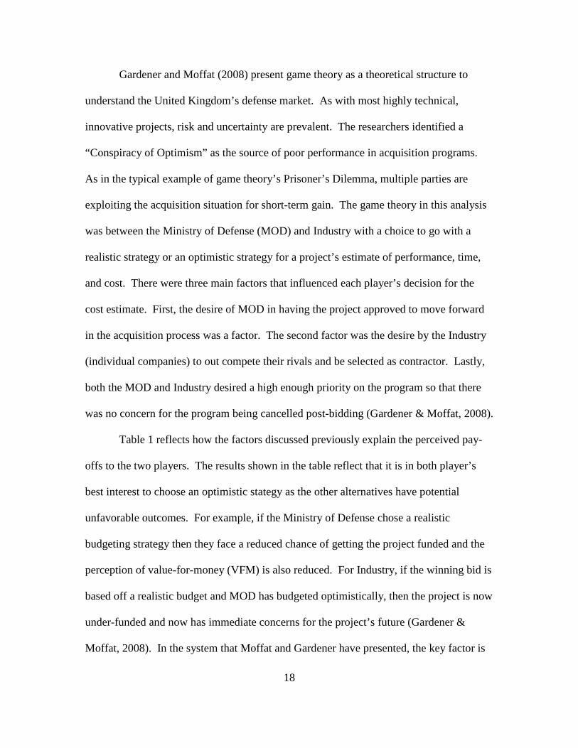
Table 1 reflects how the factors discussed previously explain the perceived pay-

offs to the two players. The results shown in the table reflect that it is in both player’s

best interest to choose an optimistic stategy as the other alternatives have potential

unfavorable outcomes. For example, if the Ministry of Defense chose a realistic

budgeting strategy then they face a reduced chance of getting the project funded and the

perception of value-for-money (VFM) is also reduced. For Industry, if the winning bid is

based off a realistic budget and MOD has budgeted optimistically, then the project is now

under-funded and now has immediate concerns for the project’s future (Gardener &

Moffat, 2008). In the system that Moffat and Gardener have presented, the key factor is

19

uncertainty. The acquisition system is full of uncertainties and is vulnerable to the

“Invasion of Optimism”. In order to ensure realistic strategies, human characteristics and

tendencies must be controlled for (Gardener & Moffat, 2008).

Table 1 - Perceived Pay-Offs to MOD and Industry

MOD budgets optimistically MOD budgets realistically Industry bids optimistically MOD

Easy entry into equipment plan (EP) (+) Favorable value-for-money (VFM) (+) Industry Easy entry into EP (+) Stay in EP (+)

MOD Difficult entry into EP (-) Bad VFM pre-bid (-) Good VFM post-bid (+) Industry Difficult entry into EP (-) Stay in EP (+)

Industry bids realistically MOD Easy entry into EP (+) Project faces cancellation (-) Industry Easy entry into EP (+) Stay in EP (+) Project faces cancellation (-)

MOD Difficult entry into EP (-) Bad VFM (-) Industry Difficult entry into EP (-) Stay in EP (+) Low risk of cancellation (+)

Source: Modified from (Gardener & Moffat, 2008)

Ritschel (2011) investigated whether game theory could be used to explain cost

variance in military weapon system contracts. The measure of cost variance used in his

analyses was based off the Defense Acquisition University’s (DAU) earned value

management gold card. Cost variance (CV) consists of subtracting the actual cost of

work performed (ACWP) from the budgeted cost of work performed (BCWP).

The program’s cost estimate is affected by the players who make up an Integrated

Product Team (IPT). The individual in charge is the Program Manager (PM) and has the

overarching goal of providing the requested capability to the requestor. Other members

of the IPT have different top priorities. The engineer may prioritize the best technical

solution, the logistics personnel may care about maintainability, budget personnel may be

20

focused only on the funding aspect, and the cost estimators may wish to constrain the

total program cost. The cost estimator formulates an estimate based off the inputs

provided by the IPT.

The Weapon System Acquisition Reform Act (WSARA) of 2009 initially

required cost estimates to be submitted with a confidence level of 80% with mandatory

reporting when a lesser confidence level was used (Public Law 111-23, 2009). This 80%

requirement was later changed (Public Law 114-328, 2016) as few projects were being

submitted at the required 80% level. Estimates were submitted closer to the 50%

confidence level as reported by the Cost Assessment and Program Evaluation (CAPE)

office. The lower confidence reporting was the result of the PM facing the difficult task

of determining an appropriate cost estimate that minimizes the chance of cost-overruns

but also still makes the program competitive for funding in the Planning, Programming,

Budgeting, and Execution (PPBE) (Ritschel, 2011).

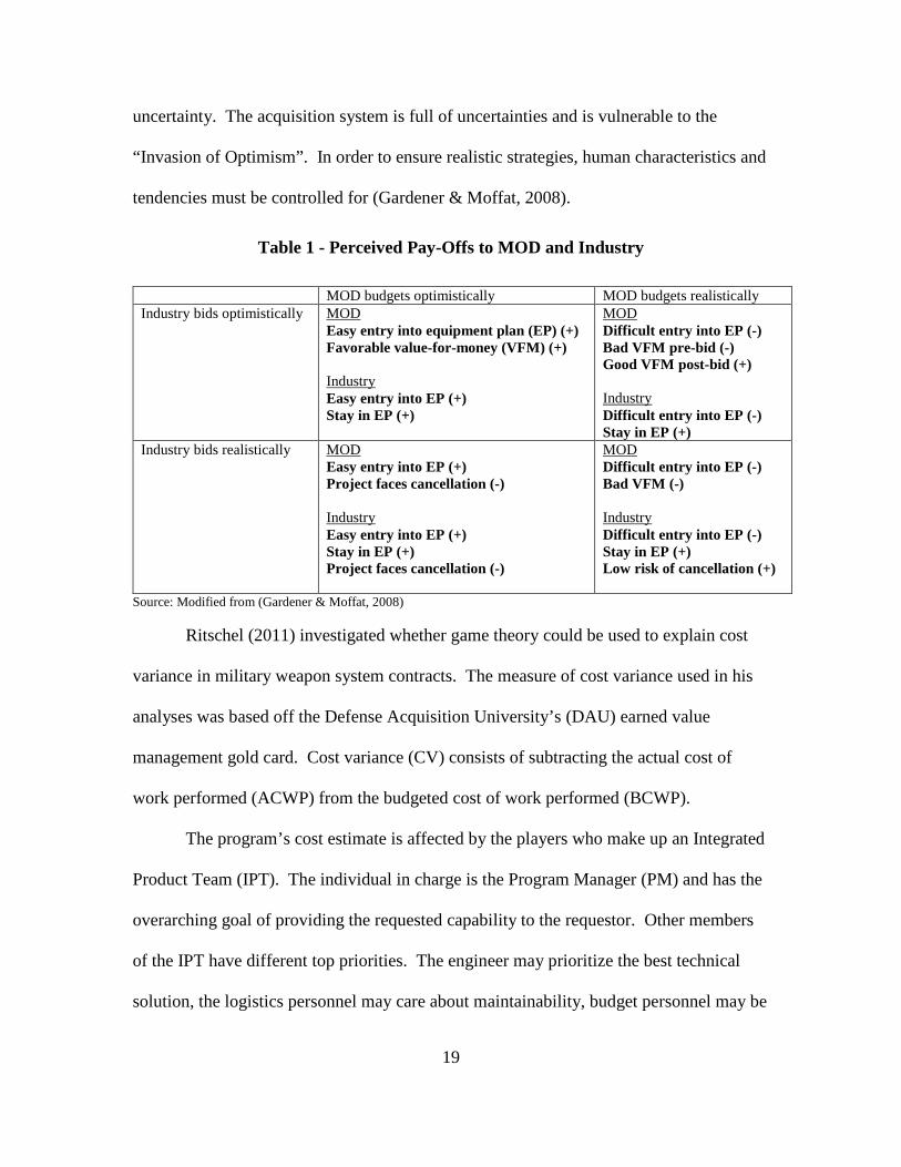
Ritschel’s analysis presented Table 2 to show three different scenarios of game

theory where the DOD has to choose whether to submit a high or low confidence budget

estimate and Congress has to decide whether they are going to fund the project. Each

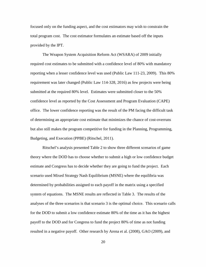
scenario used Mixed Strategy Nash Equilibrium (MSNE) where the equilibria was

determined by probabilities assigned to each payoff in the matrix using a specified

system of equations. The MSNE results are reflected in Table 3. The results of the

analyses of the three scenarios is that scenario 3 is the optimal choice. This scenario calls

for the DOD to submit a low confidence estimate 80% of the time as it has the highest

payoff to the DOD and for Congress to fund the project 80% of time as not funding

resulted in a negative payoff. Other research by Arena et al. (2008), GAO (2009), and

21

Defense Acquisition Performance Assessment Project (DAPA, 2005) supports the claim

that low confidence estimates are routinely utilized.

Table 2 - Game Theory

Source: Ritschel, 2011

Table 3 - MSNE

Source: Ritschel, 2011

The Flyvbjerg (2003), Gardener & Moffat (2008), and Ritschel (2011) analyses

provide support that game theory may factor into cost variance in the DOD acquisition

system. Flyvbjerg claims that the PMs are submitting unrealistic estimates in order to get

projects funded. This claim is supported by the consistently high cost variance present in

the 3 projects he analyzed through case studies. Moffat & Gardener presented similar

analyses using the UK’s Ministry of Defense budgeting decision and the industries

bidding decision. In their scenario, there is a dominant strategy that results in the best

outcome for both parties; however, this outcome is not necessarily the outcome with the

lowest cost. Ritschel presents a scenario where there is no dominant strategy in which

the DoD has to decide whether or not to use low or high confidence level in their cost

estimate and Congress has to decide to fund or not fund. The acquisition system is

22

complex, there are many players, and players are known to make decisions based off of

political factors.

Disconnects between policy intentions, good practices, and actual follow-through

would suggest that the DoD is going submit a cost estimate that falls around the 50%

confidence level as the goal is to get the project funded. Such a practice means there is a

high likelihood of overruns. In such an environment, it may be incumbent to take policy

action which can more strictly reduce the potential of cost growth, or contractually

preclude the growth we leave ourselves open to. Better Buying Power seems to have

taken such actions.

One method of controlling costs when there is uncertainty in the program’s

estimate is better aligning a contractor’s incentive to their performance which is the goal

of the Better Buying Power initiatives. In order for this happen, the DoD must ensure

that they establish a “credible commitment” to this behavior so that the new policies are

taken seriously.

The problem that a series of failed policy initiatives creates is a mutual lack of

faith or follow through. The signals of seriousness and competency are lost. In

Ritschell’s outcome, there is no dominant strategy. The game becomes a coordination or

brinkmanship game between the DoD and Congress in which each party is speculating

how the other might act and responds respectively. There is great uncertainty. A

coordination game is one in which multiple Nash equilibria exist. Schecter and Gintis

(2016) present examples of a coordination game. Table 4 reflects a dilemma where a

man wants to attend a wrestling event while a woman wants to attend a concert.

However, each prefers the company of the other versus attending their preferred event

23

alone as reflected by the two Nash equilibria. In this example, it is in each player best

interest to coordinate their decisions as to ensure they both receive some positive utility

(Schecter & Gintis, 2016). But the outcome is entirely unpredictable.

A second example is presented as a game of chicken (Table 5). It provides insight

into how to resolve a coordination game. Two teens are driving toward each other and a

head-on collision is imminent. Each teen wants to bolster their reputation by driving

straight. However, if they both drive straight then they are both injured. Therefore, the

only way to “win” would be to drive straight while your opponent swerves. There’s no

way to guarantee that your opponent is going to swerve so some may attempt to develop

a reputation for being “crazy” and state they are going straight no matter what and that

they don’t care if they are injured (Schecter & Gintis, 2016). Credible commitment can

more confidently resolve such uncertain speculation by signaling a certain path of action

by one player. In this case it would be the “crazy” teenager signaling that they are going

straight no matter what. Credible commitment states that when faced with a threat in a

conflict situation, the threat has to be credible in order to be effective (Schelling, 1980).

Table 4 - Battle of the Sexes Man

Concert Wrestling

Wom

an

Concert (2, 1) (0, 0)

Wrestling (0, 0) (1, 2)

Source: Modified from Schecter & Gintis, 2016

Table 5 – Chicken Teen 2

Straight Swerve

Teen

1

Straight (-2, -2) (1, -1)

Swerve (-1, 1) (0, 0) Source: Modified from Schecter & Gintis, 2016

24

Suppose that the DOD is willing to give a contractor reasonable profit in

exchange for contract performance that meets an established criterion. Both parties have

full knowledge of the outcome as long as they both fulfill their contractual obligations.

However, if the contractor believes that the government is going to pay them reasonable

profit regardless of their performance level based off of historical information then there

is no credible commitment and the contractor has no real incentive to perform their best.

Historically, this has been the case in the DoD as reported by the Government

Accountability Office’s (GAO) research in 2005, 2009, and 2017. Their 2005 research

found that the DoD paid billions in award and incentive fees regardless of acquisition

outcomes; the 2009 research found initiatives to cure the findings from 2005 were having

mixed results as they were not being consistently applied. History undermines each new

effort as weakness is presumed. The 2017 report found that the DoD did appear to be

better allocating award and incentives based on established criteria; however, the GAO

recommended better record keeping on incentive outcomes in order to maximize

effectiveness in the establishment of incentive arrangements in future contracts. The

current research provides for a different theoretical foundation from prior research.

Credible commitment promises a solution from self-serving influences. The

encouragement to use and enforce incentive contracts, if responded to, creates an

automatic mechanism for awarding profit without subjective evaluation. Incentive

contracts are a credible commitment relative to award contracts that have been budgeted

as if the award is inevitable.

25

Summary

Is it possible that the BBP initiatives are different than past initiatives? Will the

focus of aligning contractor profitability with contractor performance improve the

defense acquisition system? The next chapter, methodology, discusses how the

researchers plan to answer these questions.

26

III. Methodology

Chapter Overview

The paper provides a series of statistical tests placing profit margin as the

dependent variable. Ordinary Least Squares (OLS) regression as well as non-parametric

tests are employed to permit a time-series portrayal of the relationship of various

independent variables to profit. This is done first as a simple bivariate analysis and then

as a multivariate analysis to include Stepwise regression. Due to the nature of the

variables, the key relationship between cost variance and profit must be conducted using

contingency tables.

Data

Data was obtained from the Cost Assessment Data Enterprise (CADE). CADE’s

data is compiled from multiple authoritative databases such as Defense Automated Cost

Information Management System (DACIMS) and Defense Acquisition Management

Information Retrieval (DAMIR). The data available in CADE consists of reports such as

Contractor Cost Data Reports (CCDRs), Integrated Program Management Reports

(IPMRs), and Cost Analysis Requirements Descriptions (CARDs).

The profit data, specifically, for each contract was obtained in the form of Cost

Data Summary Reports (CDSRs) which are also often referred to as 1921s. There are

also several other types of 1921s such as the Function Cost-Hour Report (1921-1),

Progress Curve Report (1921-2), and Contractor Business Data Report (1921-3);

however, this report only focuses on the 1921.

27

The 1921 contains descriptive data such as program name, contract number,

contract type, contract price and ceiling, period of performance, report cycle (initial,

interim, or final), and cost data broken down by work breakdown structure (WBS) for

both “to date” and “at completion”. In addition to WBS elements, other costs such as

subtotal, general and administrative (G&A), undistributed budget (UB), and management

reserve (MR) are also reported. A blank 1921 is provided in Appendix A for reference.

CDSR reporting is required on ACAT I and ACAT IA programs when the

estimated contract value at completion is greater than $50 million (DoDI 5000.02).

These reports may be generated at the contract level or for a specific task or delivery

order. There are a few exceptions per DoDI 5000.02 to this reporting requirement

(Appendix B). The original database contained 2,032 final CDSRs. A CDSR is

considered final when at least 95% of the contract cost have been incurred and the

government has received its end item. The current study only views completed contracts.

The original database was analyzed for accuracy. There were 5 groups of

exclusions that were identified (Table 6). First, there were 917 subcontractor reports that

were removed as this analysis was strictly utilizing prime contractor reports.

Subcontractors have requirements that are often less stringent than primes for both profit

and earned value reporting. Next, Equation 1 was used to verify that each sample was at

least 95% complete. There were 62 data points that did not meet this threshold and were

excluded. This report focused on development and production contracts; therefore, 54

data points that were labeled as operations and sustainment (O&S) or some other life

cycle phase were excluded. Exclusion #4 was due to missing data on the 1921. The

missing data was primarily samples that did not have an accurate period of performance

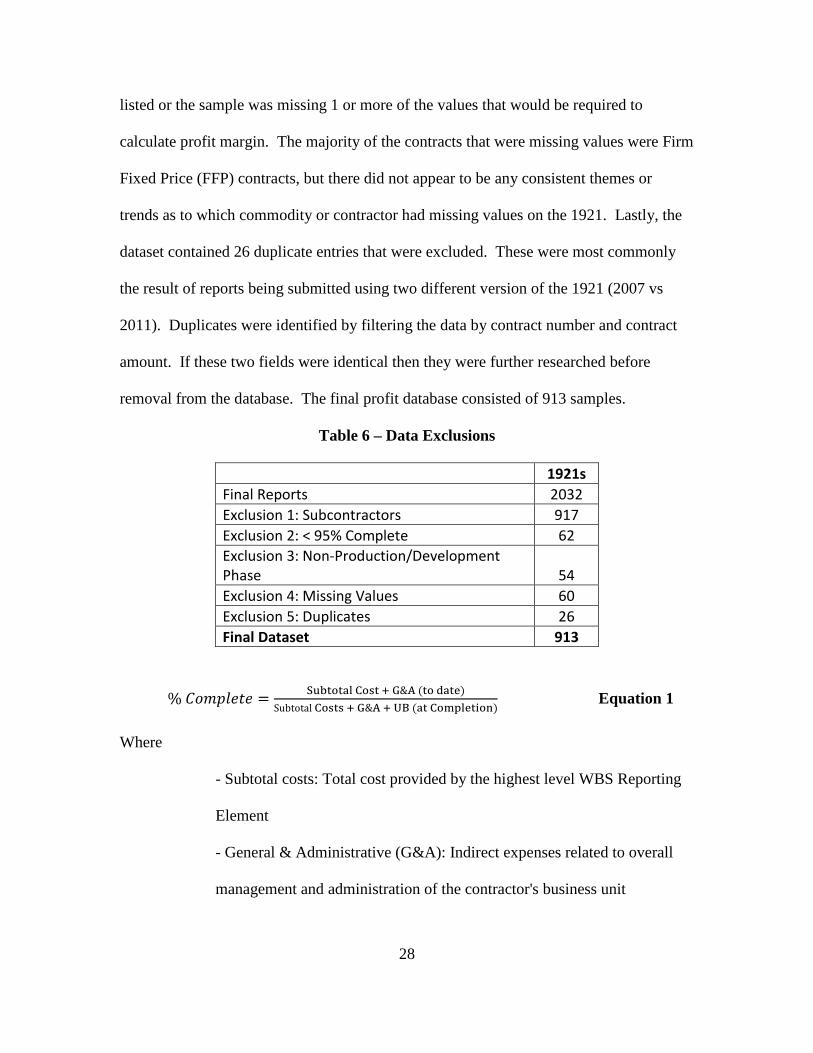
28

listed or the sample was missing 1 or more of the values that would be required to

calculate profit margin. The majority of the contracts that were missing values were Firm

Fixed Price (FFP) contracts, but there did not appear to be any consistent themes or

trends as to which commodity or contractor had missing values on the 1921. Lastly, the

dataset contained 26 duplicate entries that were excluded. These were most commonly

the result of reports being submitted using two different version of the 1921 (2007 vs

2011). Duplicates were identified by filtering the data by contract number and contract

amount. If these two fields were identical then they were further researched before

removal from the database. The final profit database consisted of 913 samples.

Table 6 – Data Exclusions

1921s Final Reports 2032 Exclusion 1: Subcontractors 917 Exclusion 2: < 95% Complete 62 Exclusion 3: Non-Production/Development Phase 54 Exclusion 4: Missing Values 60 Exclusion 5: Duplicates 26 Final Dataset 913

% 𝐶𝐶𝐶𝐶𝐶𝐶𝐶𝐶𝐶𝐶𝐶𝐶𝐶𝐶𝐶𝐶 = Subtotal Cost + G&A (to date)Subtotal Costs + G&A + UB (at Completion)

Equation 1

Where

- Subtotal costs: Total cost provided by the highest level WBS Reporting

Element

- General & Administrative (G&A): Indirect expenses related to overall

management and administration of the contractor's business unit

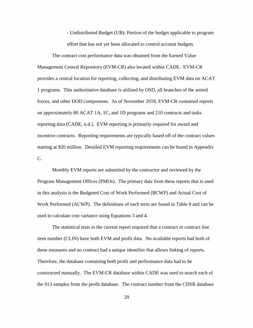
29

- Undistributed Budget (UB): Portion of the budget applicable to program

effort that has not yet been allocated to control account budgets.

The contract cost performance data was obtained from the Earned Value

Management Central Repository (EVM-CR) also located within CADE. EVM-CR

provides a central location for reporting, collecting, and distributing EVM data on ACAT

1 programs. This authoritative database is utilized by OSD, all branches of the armed

forces, and other DOD components. As of November 2018, EVM-CR contained reports

on approximately 80 ACAT 1A, 1C, and 1D programs and 210 contracts and tasks

reporting data (CADE, n.d.). EVM reporting is primarily required for award and

incentive contracts. Reporting requirements are typically based off of the contract values

starting at $20 million. Detailed EVM reporting requirements can be found in Appendix

C.

Monthly EVM reports are submitted by the contractor and reviewed by the

Program Management Offices (PMOs). The primary data from these reports that is used

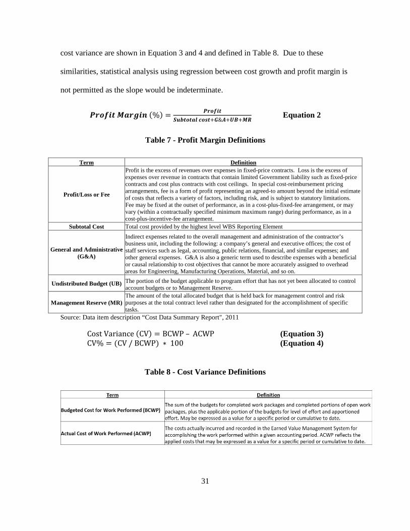
in this analysis is the Budgeted Cost of Work Performed (BCWP) and Actual Cost of

Work Performed (ACWP). The definitions of each term are found in Table 8 and can be

used to calculate cost variance using Equations 3 and 4.

The statistical tests in the current report required that a contract or contract line

item number (CLIN) have both EVM and profit data. No available reports had both of

these measures and no contract had a unique identifier that allows linking of reports.

Therefore, the database containing both profit and performance data had to be

constructed manually. The EVM-CR database within CADE was used to search each of

the 913 samples from the profit database. The contract number from the CDSR database

30

was searched in EVM-CR system. Next, CLINs, work orders, or task orders were

matched from the CDSR report name or contract task name descriptions to the EVM-CR

reports. In the event that the description from report name or contract task name was not

sufficient in matching to a specific EVM report, the subtotal cost from the CDSR and the

ACWP from the EVM were compared. If those amounts were within 5% of each other

than they were treated as possible matching reports. The periods of performance from

the two different reports were then compared for those possible matches. If they were for

the same period then they were treated as matching reports. There were 85 samples from

the profit database that had EVM reports available but they were not able to be linked

with complete certainty. The samples had the same task order but neither the amounts

nor periods of performance were similar; therefore, they had to be excluded. The final

result was a database consisting of 130 samples across unique 97 contracts that matched

to 130 samples from the CDSR database and EVM databases.

Due to limitations of the data in the current report, the relationship between cost

growth and profit margin is not easily examined. In the logical OLS format, the actual

cost of work performed (ACWP) would be on one side of the relationship and contract

subtotal cost would be on the other side. However, these amounts are fundamentally the

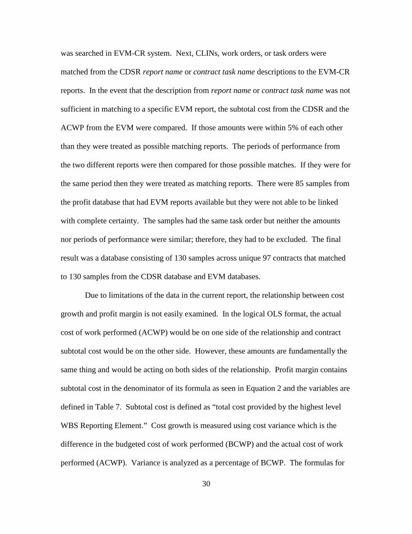
same thing and would be acting on both sides of the relationship. Profit margin contains

subtotal cost in the denominator of its formula as seen in Equation 2 and the variables are

defined in Table 7. Subtotal cost is defined as “total cost provided by the highest level

WBS Reporting Element.” Cost growth is measured using cost variance which is the

difference in the budgeted cost of work performed (BCWP) and the actual cost of work

performed (ACWP). Variance is analyzed as a percentage of BCWP. The formulas for

31

cost variance are shown in Equation 3 and 4 and defined in Table 8. Due to these

similarities, statistical analysis using regression between cost growth and profit margin is

not permitted as the slope would be indeterminate.

𝑷𝑷𝑷𝑷𝑷𝑷𝑷𝑷𝑷𝑷𝑷𝑷 𝑴𝑴𝑴𝑴𝑷𝑷𝑴𝑴𝑷𝑷𝑴𝑴 (%) = 𝑷𝑷𝑷𝑷𝑷𝑷𝑷𝑷𝑷𝑷𝑷𝑷𝑺𝑺𝑺𝑺𝑺𝑺𝑷𝑷𝑷𝑷𝑷𝑷𝑴𝑴𝑺𝑺 𝒄𝒄𝑷𝑷𝒄𝒄𝑷𝑷+𝑮𝑮&𝑨𝑨+𝑼𝑼𝑼𝑼+𝑴𝑴𝑴𝑴

Equation 2

Table 7 - Profit Margin Definitions

Term Definition

Profit/Loss or Fee

Profit is the excess of revenues over expenses in fixed-price contracts. Loss is the excess of expenses over revenue in contracts that contain limited Government liability such as fixed-price contracts and cost plus contracts with cost ceilings. In special cost-reimbursement pricing arrangements, fee is a form of profit representing an agreed-to amount beyond the initial estimate of costs that reflects a variety of factors, including risk, and is subject to statutory limitations. Fee may be fixed at the outset of performance, as in a cost-plus-fixed-fee arrangement, or may vary (within a contractually specified minimum maximum range) during performance, as in a cost-plus-incentive-fee arrangement.

Subtotal Cost Total cost provided by the highest level WBS Reporting Element

General and Administrative (G&A)

Indirect expenses related to the overall management and administration of the contractor’s business unit, including the following: a company’s general and executive offices; the cost of staff services such as legal, accounting, public relations, financial, and similar expenses; and other general expenses. G&A is also a generic term used to describe expenses with a beneficial or causal relationship to cost objectives that cannot be more accurately assigned to overhead areas for Engineering, Manufacturing Operations, Material, and so on.

Undistributed Budget (UB) The portion of the budget applicable to program effort that has not yet been allocated to control account budgets or to Management Reserve.

Management Reserve (MR) The amount of the total allocated budget that is held back for management control and risk purposes at the total contract level rather than designated for the accomplishment of specific tasks.

Source: Data item description “Cost Data Summary Report", 2011

Cost Variance (CV) = BCWP – ACWP (Equation 3) CV% = (CV / BCWP) ∗ 100 (Equation 4)

Table 8 - Cost Variance Definitions

32

Due to the previously mentioned limitations in comparing profit margin and cost

variance, other variables are analyzed in order to determine their significance in

predicting profit margin. In a few instances, variables are also tested against a dependent

variable for cost growth in order to provide a more holistic view of the analysis. These

variables fall into 1 of 3 categories: technical, economical, or environmental.

Technical variables are primarily categorical variables that are obtained from the

contractor’s Cost Data Summary Report (CDSR). They are as follows:

• Commodity

• Branch of Service

• Contractor

• Life Cycle Phase

• Contract Type

• Incentive Structure

• Period of Performance Start Year

This paper does not analyze in detail each of these variables as most are not

significant predictors; however, a detailed listing for each variable is provided in

Appendix D through I that contains the sample size, mean cost variance, and mean profit

margin for the variable with regard to all years, the years before 2011, and the years after

2010.

Most of the variables are self-explanatory and will be discussed as needed

throughout the analysis. However, the two variables for profit structure and contract type

require further clarification. Contract type originally contained 16 unique inputs when

pulled from the CDSRs. These inputs were condensed into contract types of Cost, Fixed,

33

and Mixed. Mixed samples are those containing multiple CLINs or work orders with

both a cost and fixed type of contract. The same listing was also used to create variables

for profit structure. Variables of “IF” for incentive fee or “AF” for award fee established.

There were 8 samples that contained both incentive and award fee structures and 28

samples where the 1921 did not indicate either type.

Two of the primary technical variables that are analyzed are the period of

performance start year and incentive structure. The period of performance start year is

important for the time-series part of the analysis. In order to determine if Better Buying

Power has been effective, a binary variable was created that would result in ‘1’ if the

period of performance start year was greater than 2010 and would result in ‘0’ if not. The

second key variable was profit structure. The profit structure could either be incentive

fee (IF), award fee (AF), both incentive and award, or neither incentive or award.

Separate binary variables were created for both IF and AF where the result would be a ‘1’

if the sample was strictly IF or AF and a ‘0’ if not. The time and profit structure

variables can be directly linked to specific aspects of Better Buying Power and may

provide the most measurable insight in analyzing whether Better Buying Power has been

implemented effectively.

Economic variables were also included to test whether it’s a changing economy

that is resulting in increasing profit margins or if the changes may be the result of some

other factor such as the implementation of Better Buying Power. Economic variables for

the gross domestic product rate change from prior year, federal funds rate, unemployment

rate, and the service’s budget during the year of contract performance start. The rates for

each variable are associated with the period of performance start year. The data for each

34

variable was obtained from authoritative sources such as the Bureau of Economic

Analyses, Federal Reserve website, and the President’s Budget.

Environmental variables were analyzed to account for signals that contractors

may have received from prior knowledge of DoD acquisitions. They are all exploratory

in nature. They are proxies designed to capture the influence of observable signals to the

contractor that the government is serious. These variables are included as an extension of

game theory; whereas, a coordination game is resolve through one agent picking up a

signal of credible commitment. As such, variables for the median profit from prior years

are introduced into the model. One variable captures the prior year median profit margin

for the EVM only contracts (130 samples) while another variable captures the median

profit margin from the larger, non-EVM dataset (913 samples). The variables derived

from the larger dataset excluded the 130 samples used in the smaller dataset. The theory

is that contactors are aware of the overall DoD climate of profit and it may influence their

behavior.

Statistical Analysis

The intent of a profit incentive is to adequately reward a contractor for their

performance. Performance is normally measured in terms of technicality, cost, and

schedule. This analysis is only focused on cost performance in the form of cost

variance/growth. The hypothesis would be that cost growth declines (increases) as profit

margin increases (decreases). This thesis has 3 research questions which are as follows:

1. What trends of profit margin and cost growth are observed over time?

35

2. Does the relationship between profit margin and cost growth, relative to

BBP’s initiation in 2010, change in such a way that would lead one to

identify an independent effect from other changes within the DoD

environment?

3. To what degree can we attribute changes in profit and performance to the

larger economy, program aspects, and overall policy?

In order to assess trends over time for the first research question, OLS regression

is used to fit a regression line using profit margin as a dependent variable and the start

year of the period of performance (POP) as an independent variable. The same process is

done using cost variance as a dependent variable and time as the independent variable.

Additionally, these same trends are examined for both incentive only contracts and non-

incentive contracts. All statistical tests in this analysis use an alpha of 0.05.

The second research question looks to examine the relationship of profit margin

and cost growth relative to the year 2010 when BBP was initiated. If BBP has been

affective then we would expect to see cost growth declining post-2010 and profit margin

increasing post-2010. In addition, BBP encouraged the use of incentive structured

contracts vs award structures. We’d expect to see an increase in the incentive type

contract post-2010 and a reduction in award type contracts. For this part of the research,

bivariate, non-parametric analysis is used with profit margin as a dependent variable and

also with cost variance as a dependent variable. The independent variables used were all

binary, dummy variables. The first dummy variable used was based off of the POP start

year. The second variable was based on the profit structure. The Wilcoxon Test is used

to test whether the differences in the medians is significant using an alpha of 0.05.

36

The analysis for research question #3 has 3 parts. First, a one-way analysis of

variance (ANOVA) is used to test the significance of the economic variables. The

environmental variables were also explored using a one-way ANOVA. If the p-value

from the ANOVAs is less than 0.05 than the tested variable is considered to be a

significant predictor of profit martin or cost variance.

The second part of the analysis utilized Stepwise Regression to determine the

best-fitting model using all technical, economic, and environmental variables. The intent

of the model is not to predict future profit margin. Instead, it is used to determine how

much of the variance can be explained. Since cost variance cannot be used as an

independent variable with profit margin, we would expect the model to have a large

amount of unexplained variance (low r-squared). The theory is that performance as an

independent variable would be able to explain more of the observed variance. This

regression model is tested for normality using a Shapiro Wilk Goodness-of-Fit Test and

constant variance using Breusch-Pagan Test. In addition, studentized residuals are used

to explore potential outliers and Cook’s Distance is used to explore any overly influential

data points.

Due to the limitations mentioned previously with using regression to relate profit

margin and cost variance, contingency tables were used. A contingency table is a

statistical tool that allows for the analysis of the relationship between at least two nominal

variables using rows and columns. The table provides for probability-related calculations

in order to confirm whether two variables are truly independent. The current research

used the median profit margin before 2011 (9.79%) and the mean cost variance % prior to

2011 (1.14%) in order to establish binary, categorical variables. If the median profit

37

margin or median cost variance was greater than the median of the data prior to 2011 then

it received a ‘1’ while everything less than the median during the same period would be

labeled a ‘0’.

Pearson’s Chi-Squared Test and the Odds-Ratio Test for significance are more

commonly used tests for independence. However, these tests require larger sample sizes

to support the p-value approximation that is provides. The current research utilizes

Fisher’s Exact Test as it is preferred when dealing with smaller sample sizes. One benefit

to the Fisher’s Exact Test is that it provides an exact calculation of a p-value given the

data presented (Agresti, 1992).

Fisher’s Exact can be used for both 1 and 2-tailed hypothesis tests. However, the

current research uses only a 1-tailed test to test the relationship between cost growth (x)

and profit margin (y). The hypothesis for a left-tailed test is as follows:

Ho: The median CV% and profit % are independent of each other

Ha: The probability (sample profit margin > than the median profit margin prior to

2011) is greater when the observed CV% is less than the median CV% prior to

2011

For the current research, the p-value for the left-tailed test is expected to be less

than 0.05. This would signal that cost growth and profit margin are not independent. If

this hypothesis is true then that would further support the claim that Better Buying Power

has been effective in improving the DoD acquisition community by bettering aligning

profitability and performance.

Lastly, sensitivity analysis was performed in order to determine if the observed

trends post-2010 are due to Better Buying Power or if it’s possible that the acquisition

38

environment was already improving. The dummy variable for the Period of Performance

Start Year was adjusted to use 2008 as a reference point. Anything after 2008 would be

coded a ‘1’ and anything prior to 2009 would be labeled a ‘0’. The same non-parametric

and regression tests that were utilized previously were used with this new time variable.

If the acquisition environment was already improving in 2008 then we cannot say with

complete certainty that the observed changes after 2010 are the direct result of BBP.

Summary

Chapter 3 has discussed the sources of the data used in the current research. In

addition, the methods of combining the profit and performance databases were described.

Next, statistical analysis using non-parametrics, OLS regression, and contingency tables

is discussed. The results of these tests are discussed in Chapter 4.

39

IV. Analysis and Results

Overview

The Office of the Under Secretary of Defense (OUSD) for Acquisition,

Technology, and Logistics (AT&L) has recently reported reduced cost variance on earned

value contracts (Davis & Anton, 2016). The positive trends that are presented in this

chapter may be capturing what the acquisition community has aimed for with the

implementation of Better Buying Power. These results reflect that the DoD may be

willing to pay a higher profit in exchange for better performance on contracts. This

chapter looks to examine what trends, if any, are reflected in the data, how has profit

margin and the use of incentive contracts changed since the implementation of Better

Buying Power in 2010, and to what degree can we relate the observed changes to Better

Buying Power? The current research aims to link profit and performance into one

analysis and determine whether the reduced cost variance occurs with contracts that

receive higher profit margins over the 2001-2016 timeframe, or whether it is an artifact of

some other driver.

This chapter discusses the analysis and results starting with descriptive statistics.

Next, the results of the non-parametric and ordinary least squares (OLS) regression are

discussed and significant correlations of profit margin are identified. The correlations

fall into 3 categories: technical, economical, and environmental. Economic and

environmental variables are introduced into the regression in order to test the effect that

each one may have on profit margin as it could potentially be factors outside of the DoD

that are responsible for the acquisition improvements. Contingency tables are introduced

40

along with their results in order to examine the relationship between profit margin and

cost variance together. Finally, the sensitivity analysis is discussed.

Descriptive Statistics

The database consisted of the following 6 categorical variables: commodity,

branch of service, contract type, incentive structure, contractor, and contract phase. The

distributions of each of these variables in shown in Table 9 and the mean profit margins

and cost variances for each can be found in Appendix D through Appendix I. Some

variables were not used in the analysis but their distributions are provided in the

Appendix to allow for a more complete picture of the database.

Descriptive statistics in the data set are broken down into 3 groups: all years, pre-

2011, and post-2010. The dataset of 130 samples had a median cost variance of 0.99%

and a median profit margin 13.21% when all years are included (Table 9). The cost

variance reported is not as high as others have reported e.g. Drezner et al. (1993).

Drezner examined program SARs from 1960-1990 in his analysis and found the mean

cost growth to be around 20%. The difference between the current research and

Drezner’s research is likely due to the current research focusing on specific CLINs and

work orders while Drezner looked at program level data from the Selected Acquisition

Reports (SARs).

41

Table 9- Variable Distributions

Total Samples 130

Commodity # Profit

Structure # Aircraft 44 Incentive 72 Ship 24 Neither 28 UAV 22 Award Fee 22 Electronic/Automated Software 19 Both 8

Missiles 12 Contract

Type # Space 5 Cost 72 Ordinance 2 Fixed 51 Surface Vehicle 2 Mixed 7

Service # Phase # Navy 74 Production 73 Air Force 30 Development 57 Army 21 Contractor # DoD (Joint) 5 Contractor A 20

POP Start Year # Contractor B 19

2001 3 Contractor C 14 2003 4 Contractor D 13 2004 3 Contractor E 12 2005 3 Contractor F 10 2006 12 Contractor G 9 2007 13 Contractor H 6 2008 11 Contractor I 5 2009 12 Contractor J 5 2010 17 Contractor K 3 2011 12 Contractor L 3 2012 15 Contractor M 2 2013 12 Contractor N 2 2014 8 Contractor O 2 2015 4 Contractor P 2 2016 1 Contractor Q 1

<2011 78 Contractor R 1 >2010 52 Contractor S 1

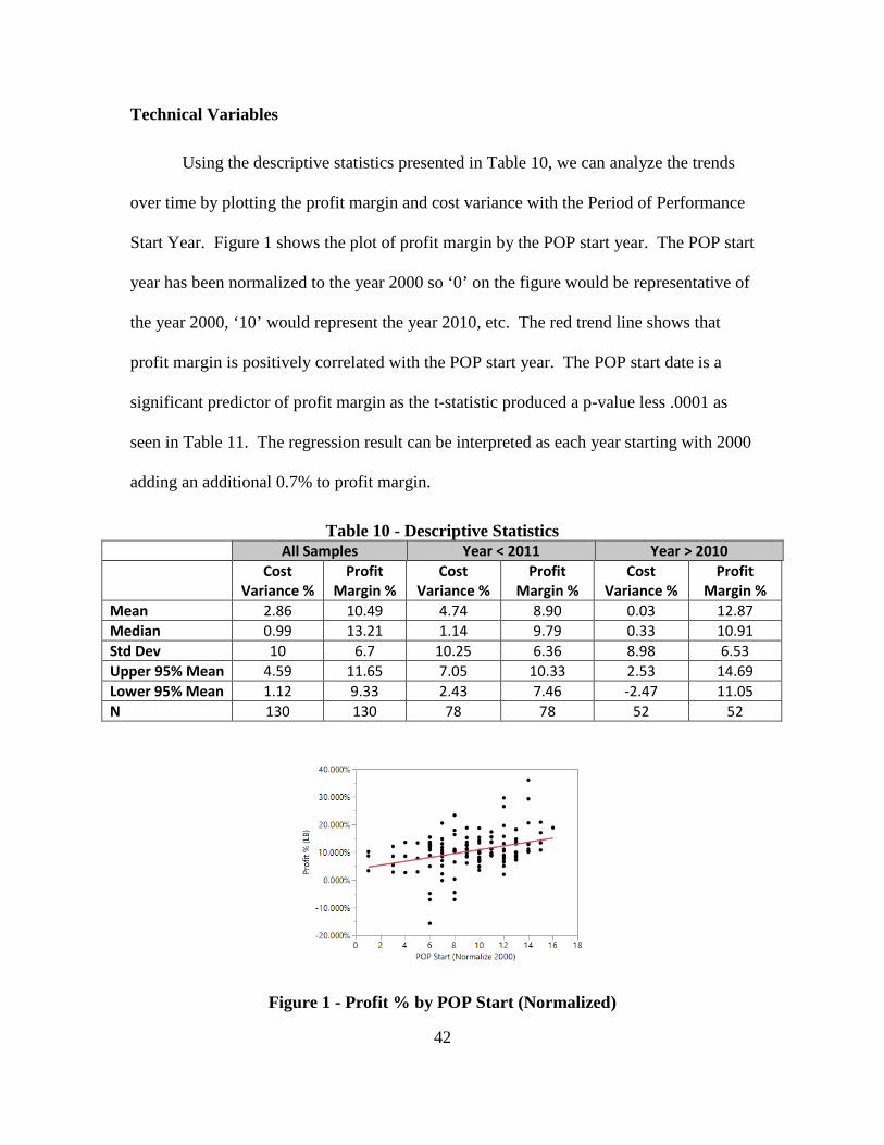
42

Technical Variables

Using the descriptive statistics presented in Table 10, we can analyze the trends

over time by plotting the profit margin and cost variance with the Period of Performance

Start Year. Figure 1 shows the plot of profit margin by the POP start year. The POP start

year has been normalized to the year 2000 so ‘0’ on the figure would be representative of

the year 2000, ‘10’ would represent the year 2010, etc. The red trend line shows that

profit margin is positively correlated with the POP start year. The POP start date is a

significant predictor of profit margin as the t-statistic produced a p-value less .0001 as

seen in Table 11. The regression result can be interpreted as each year starting with 2000

adding an additional 0.7% to profit margin.

Table 10 - Descriptive Statistics All Samples Year < 2011 Year > 2010 Cost

Variance % Profit

Margin % Cost

Variance % Profit

Margin % Cost

Variance % Profit

Margin % Mean 2.86 10.49 4.74 8.90 0.03 12.87 Median 0.99 13.21 1.14 9.79 0.33 10.91 Std Dev 10 6.7 10.25 6.36 8.98 6.53 Upper 95% Mean 4.59 11.65 7.05 10.33 2.53 14.69 Lower 95% Mean 1.12 9.33 2.43 7.46 -2.47 11.05 N 130 130 78 78 52 52

Figure 1 - Profit % by POP Start (Normalized)

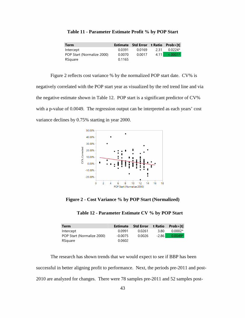
43

Table 11 - Parameter Estimate Profit % by POP Start

Term Estimate Std Error t Ratio Prob>|t| Intercept 0.0391 0.0169 2.31 0.0224* POP Start (Normalize 2000) 0.0070 0.0017 4.11 <.0001* RSquare 0.1165

Figure 2 reflects cost variance % by the normalized POP start date. CV% is

negatively correlated with the POP start year as visualized by the red trend line and via

the negative estimate shown in Table 12. POP start is a significant predictor of CV%

with a p-value of 0.0049. The regression output can be interpreted as each years’ cost

variance declines by 0.75% starting in year 2000.

Figure 2 - Cost Variance % by POP Start (Normalized)

Table 12 - Parameter Estimate CV % by POP Start

Term Estimate Std Error t Ratio Prob>|t| Intercept 0.0991 0.0261 3.80 0.0002* POP Start (Normalize 2000) -0.0075 0.0026 -2.86 0.0049* RSquare 0.0602

The research has shown trends that we would expect to see if BBP has been

successful in better aligning profit to performance. Next, the periods pre-2011 and post-

2010 are analyzed for changes. There were 78 samples pre-2011 and 52 samples post-

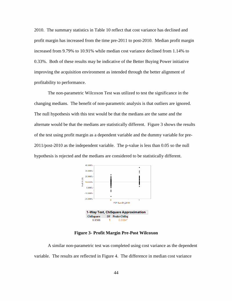
44

2010. The summary statistics in Table 10 reflect that cost variance has declined and

profit margin has increased from the time pre-2011 to post-2010. Median profit margin

increased from 9.79% to 10.91% while median cost variance declined from 1.14% to

0.33%. Both of these results may be indicative of the Better Buying Power initiative

improving the acquisition environment as intended through the better alignment of

profitability to performance.

The non-parametric Wilcoxon Test was utilized to test the significance in the

changing medians. The benefit of non-parametric analysis is that outliers are ignored.

The null hypothesis with this test would be that the medians are the same and the

alternate would be that the medians are statistically different. Figure 3 shows the results

of the test using profit margin as a dependent variable and the dummy variable for pre-

2011/post-2010 as the independent variable. The p-value is less than 0.05 so the null

hypothesis is rejected and the medians are considered to be statistically different.

Figure 3- Profit Margin Pre-Post Wilcoxon

A similar non-parametric test was completed using cost variance as the dependent

variable. The results are reflected in Figure 4. The difference in median cost variance

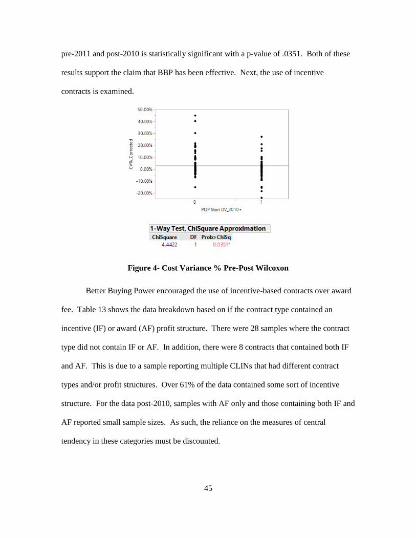
45

pre-2011 and post-2010 is statistically significant with a p-value of .0351. Both of these

results support the claim that BBP has been effective. Next, the use of incentive

contracts is examined.

Figure 4- Cost Variance % Pre-Post Wilcoxon

Better Buying Power encouraged the use of incentive-based contracts over award

fee. Table 13 shows the data breakdown based on if the contract type contained an

incentive (IF) or award (AF) profit structure. There were 28 samples where the contract

type did not contain IF or AF. In addition, there were 8 contracts that contained both IF

and AF. This is due to a sample reporting multiple CLINs that had different contract

types and/or profit structures. Over 61% of the data contained some sort of incentive

structure. For the data post-2010, samples with AF only and those containing both IF and

AF reported small sample sizes. As such, the reliance on the measures of central

tendency in these categories must be discounted.

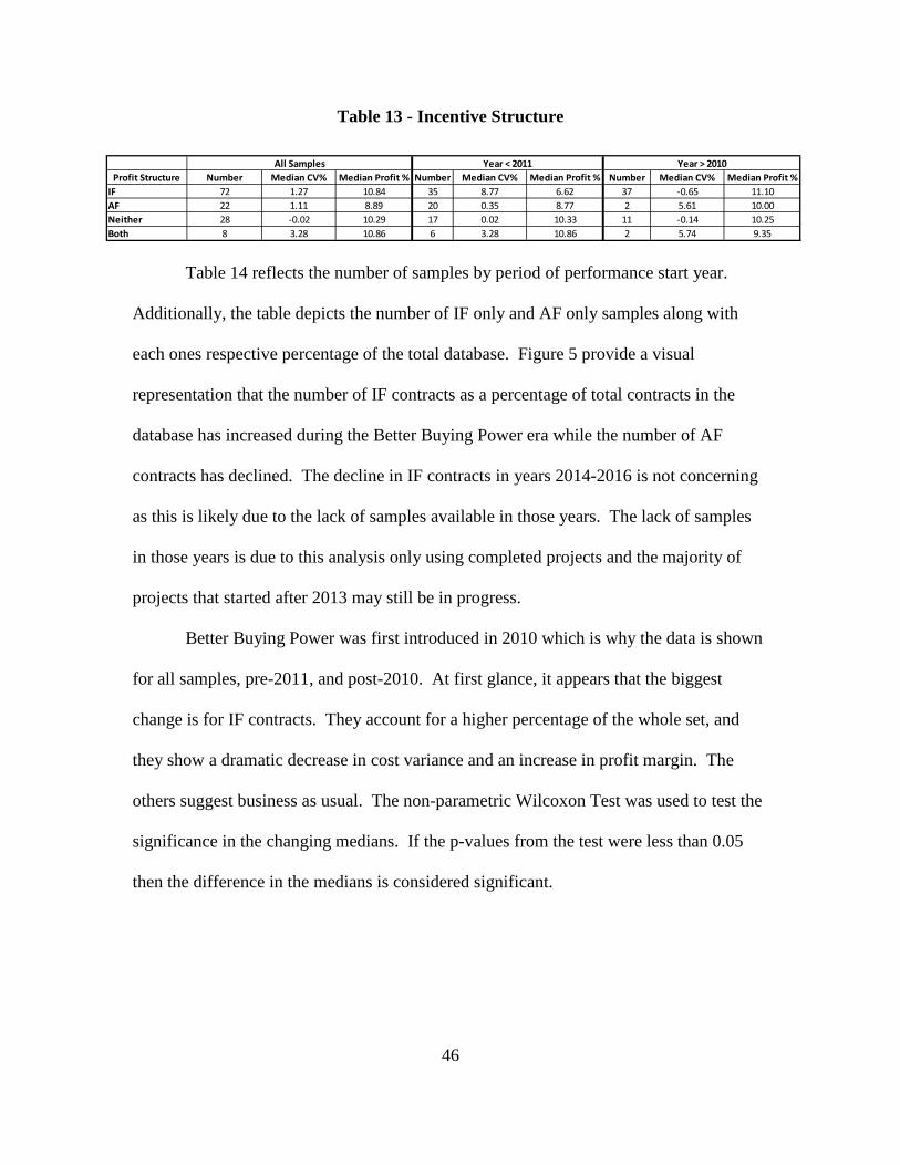
46

Table 13 - Incentive Structure

Table 14 reflects the number of samples by period of performance start year.

Additionally, the table depicts the number of IF only and AF only samples along with

each ones respective percentage of the total database. Figure 5 provide a visual

representation that the number of IF contracts as a percentage of total contracts in the

database has increased during the Better Buying Power era while the number of AF

contracts has declined. The decline in IF contracts in years 2014-2016 is not concerning

as this is likely due to the lack of samples available in those years. The lack of samples

in those years is due to this analysis only using completed projects and the majority of

projects that started after 2013 may still be in progress.

Better Buying Power was first introduced in 2010 which is why the data is shown

for all samples, pre-2011, and post-2010. At first glance, it appears that the biggest

change is for IF contracts. They account for a higher percentage of the whole set, and

they show a dramatic decrease in cost variance and an increase in profit margin. The

others suggest business as usual. The non-parametric Wilcoxon Test was used to test the

significance in the changing medians. If the p-values from the test were less than 0.05

then the difference in the medians is considered significant.

Profit Structure Number Median CV% Median Profit % Number Median CV% Median Profit % Number Median CV% Median Profit %IF 72 1.27 10.84 35 8.77 6.62 37 -0.65 11.10AF 22 1.11 8.89 20 0.35 8.77 2 5.61 10.00Neither 28 -0.02 10.29 17 0.02 10.33 11 -0.14 10.25Both 8 3.28 10.86 6 3.28 10.86 2 5.74 9.35

All Samples Year < 2011 Year > 2010

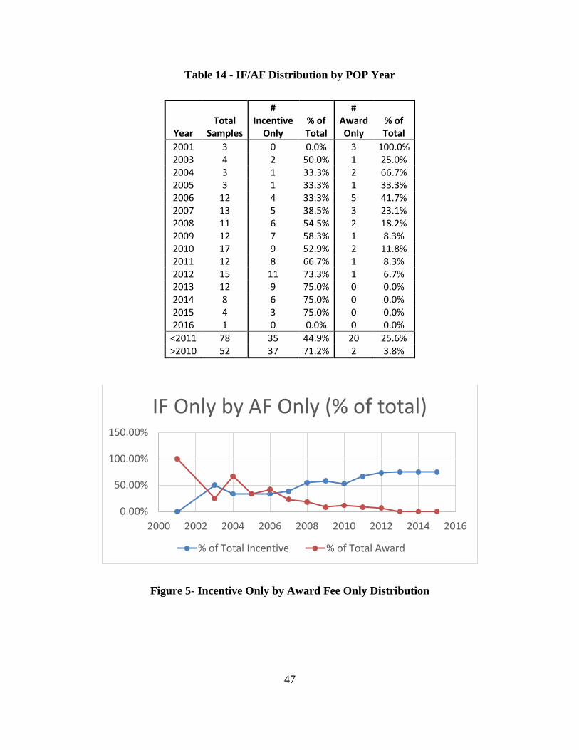
47

Table 14 - IF/AF Distribution by POP Year

Year Total

Samples

# Incentive

Only % of Total

# Award Only

% of Total

2001 3 0 0.0% 3 100.0% 2003 4 2 50.0% 1 25.0% 2004 3 1 33.3% 2 66.7% 2005 3 1 33.3% 1 33.3% 2006 12 4 33.3% 5 41.7% 2007 13 5 38.5% 3 23.1% 2008 11 6 54.5% 2 18.2% 2009 12 7 58.3% 1 8.3% 2010 17 9 52.9% 2 11.8% 2011 12 8 66.7% 1 8.3% 2012 15 11 73.3% 1 6.7% 2013 12 9 75.0% 0 0.0% 2014 8 6 75.0% 0 0.0% 2015 4 3 75.0% 0 0.0% 2016 1 0 0.0% 0 0.0%

<2011 78 35 44.9% 20 25.6% >2010 52 37 71.2% 2 3.8%

Figure 5- Incentive Only by Award Fee Only Distribution

0.00%

50.00%

100.00%

150.00%

2000 2002 2004 2006 2008 2010 2012 2014 2016

IF Only by AF Only (% of total)

% of Total Incentive % of Total Award

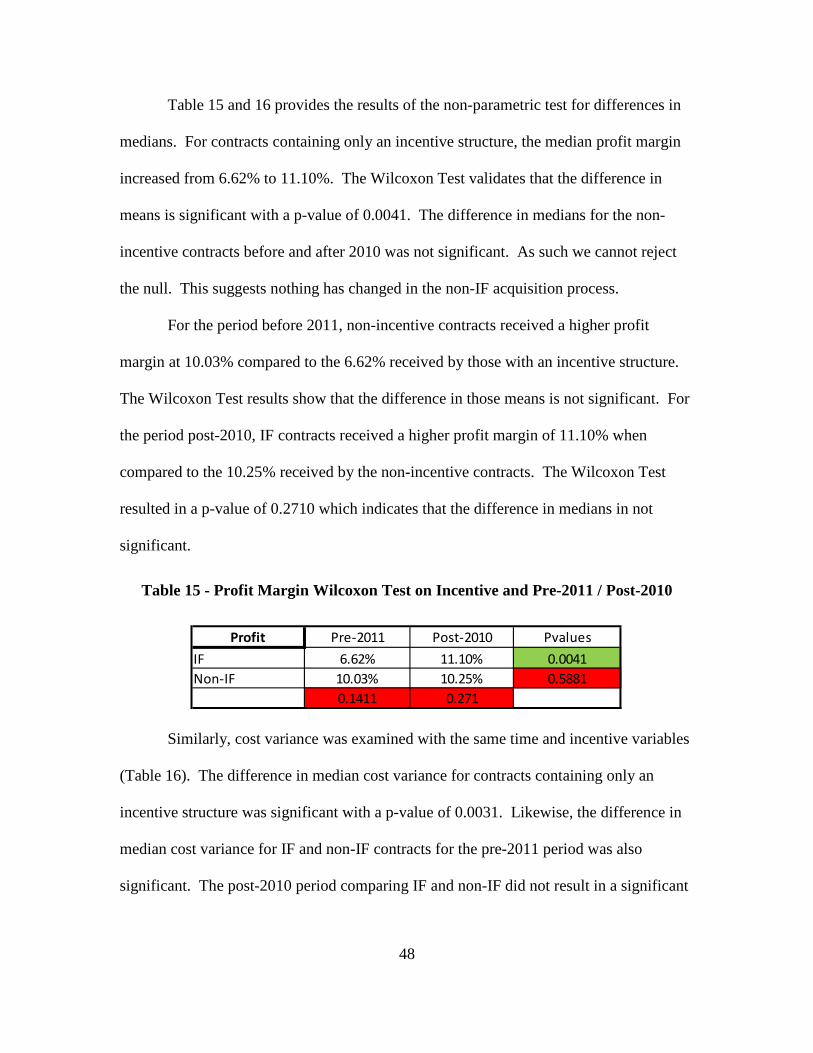
48

Table 15 and 16 provides the results of the non-parametric test for differences in

medians. For contracts containing only an incentive structure, the median profit margin

increased from 6.62% to 11.10%. The Wilcoxon Test validates that the difference in

means is significant with a p-value of 0.0041. The difference in medians for the non-

incentive contracts before and after 2010 was not significant. As such we cannot reject

the null. This suggests nothing has changed in the non-IF acquisition process.

For the period before 2011, non-incentive contracts received a higher profit

margin at 10.03% compared to the 6.62% received by those with an incentive structure.

The Wilcoxon Test results show that the difference in those means is not significant. For

the period post-2010, IF contracts received a higher profit margin of 11.10% when

compared to the 10.25% received by the non-incentive contracts. The Wilcoxon Test

resulted in a p-value of 0.2710 which indicates that the difference in medians in not

significant.

Table 15 - Profit Margin Wilcoxon Test on Incentive and Pre-2011 / Post-2010

Similarly, cost variance was examined with the same time and incentive variables

(Table 16). The difference in median cost variance for contracts containing only an

incentive structure was significant with a p-value of 0.0031. Likewise, the difference in

median cost variance for IF and non-IF contracts for the pre-2011 period was also

significant. The post-2010 period comparing IF and non-IF did not result in a significant

Profit Pre-2011 Post-2010 PvaluesIF 6.62% 11.10% 0.0041Non-IF 10.03% 10.25% 0.5881

0.1411 0.271

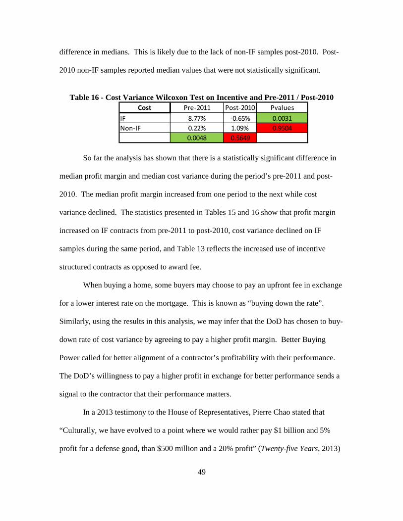
49

difference in medians. This is likely due to the lack of non-IF samples post-2010. Post-

2010 non-IF samples reported median values that were not statistically significant.

Table 16 - Cost Variance Wilcoxon Test on Incentive and Pre-2011 / Post-2010

So far the analysis has shown that there is a statistically significant difference in

median profit margin and median cost variance during the period’s pre-2011 and post-

2010. The median profit margin increased from one period to the next while cost

variance declined. The statistics presented in Tables 15 and 16 show that profit margin

increased on IF contracts from pre-2011 to post-2010, cost variance declined on IF

samples during the same period, and Table 13 reflects the increased use of incentive

structured contracts as opposed to award fee.

When buying a home, some buyers may choose to pay an upfront fee in exchange

for a lower interest rate on the mortgage. This is known as “buying down the rate”.

Similarly, using the results in this analysis, we may infer that the DoD has chosen to buy-

down rate of cost variance by agreeing to pay a higher profit margin. Better Buying

Power called for better alignment of a contractor’s profitability with their performance.

The DoD’s willingness to pay a higher profit in exchange for better performance sends a

signal to the contractor that their performance matters.

In a 2013 testimony to the House of Representatives, Pierre Chao stated that

“Culturally, we have evolved to a point where we would rather pay $1 billion and 5%

profit for a defense good, than $500 million and a 20% profit” (Twenty-five Years, 2013)

Cost Pre-2011 Post-2010 PvaluesIF 8.77% -0.65% 0.0031Non-IF 0.22% 1.09% 0.9504

0.0048 0.5649

50

Increased profit margins are not to be seen as a negative for the DoD. Former Under

Secretary of Defense for AT&L, Frank Kendall, argued that capitalism results in

industries striving to maximize profit. The DoD has the responsibility of both protecting

taxpayer’s interests but also ensuring fair treatment of industry partners. Without

reasonable profit, the industries have no incentive to work with the DoD. Kendall also

contends “we (DoD) will benefit if profit incentives provide effective motivation to

industry and are tied to the goals we value” (Kendall, 2015).

Economic Variables

As discussed in Chapter 2, acquisition reforms have not always been successful or

shown results as originally intended. For the current research, it is possible that a

changing economy or other factor outside of the DoD’s control have been the reason for

profit margin’s increasing while cost variance has decreased. In order to account for

these economic conditions, the following variables were tested:

• Gross Domestic Product % Change Year Prior to POP Start

• Federal Fund Rate of the POP Start Year

• Unemployment Rate of the POP Start Year

• Service’s Budget of the POP Start Year

When analyzing these economic variables with profit margin, the only significant

variable was the Federal Fund rate with a p-value of 0.0097 and an R-square of 0.0511

(Table 17). There was negative correlation between the Fed Fund rate and profit margin

so as the rate increases, profit margins declined. This variable by itself does not explain

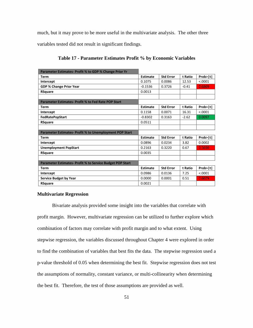
51

much, but it may prove to be more useful in the multivariate analysis. The other three

variables tested did not result in significant findings.

Table 17 - Parameter Estimates Profit % by Economic Variables

Parameter Estimates- Profit % to GDP % Change Prior Yr Term Estimate Std Error t Ratio Prob>|t| Intercept 0.1075 0.0086 12.53 <.0001 GDP % Change Prior Year -0.1536 0.3726 -0.41 0.6809 RSquare 0.0013

Parameter Estimates- Profit % to Fed Rate POP Start Term Estimate Std Error t Ratio Prob>|t| Intercept 0.1158 0.0071 16.31 <.0001 FedRatePopStart -0.8302 0.3163 -2.62 0.0097 RSquare 0.0511

Parameter Estimates- Profit % to Unemployment POP Start Term Estimate Std Error t Ratio Prob>|t| Intercept 0.0896 0.0234 3.82 0.0002 Unemployment PopStart 0.2163 0.3220 0.67 0.5030 RSquare 0.0035

Parameter Estimates- Profit % to Service Budget POP Start Term Estimate Std Error t Ratio Prob>|t| Intercept 0.0986 0.0136 7.25 <.0001 Service Budget by Year 0.0000 0.0001 0.51 0.6079 RSquare 0.0021

Multivariate Regression

Bivariate analysis provided some insight into the variables that correlate with

profit margin. However, multivariate regression can be utilized to further explore which

combination of factors may correlate with profit margin and to what extent. Using

stepwise regression, the variables discussed throughout Chapter 4 were explored in order

to find the combination of variables that best fits the data. The stepwise regression used a

p-value threshold of 0.05 when determining the best fit. Stepwise regression does not test

the assumptions of normality, constant variance, or multi-collinearity when determining

the best fit. Therefore, the test of those assumptions are provided as well.

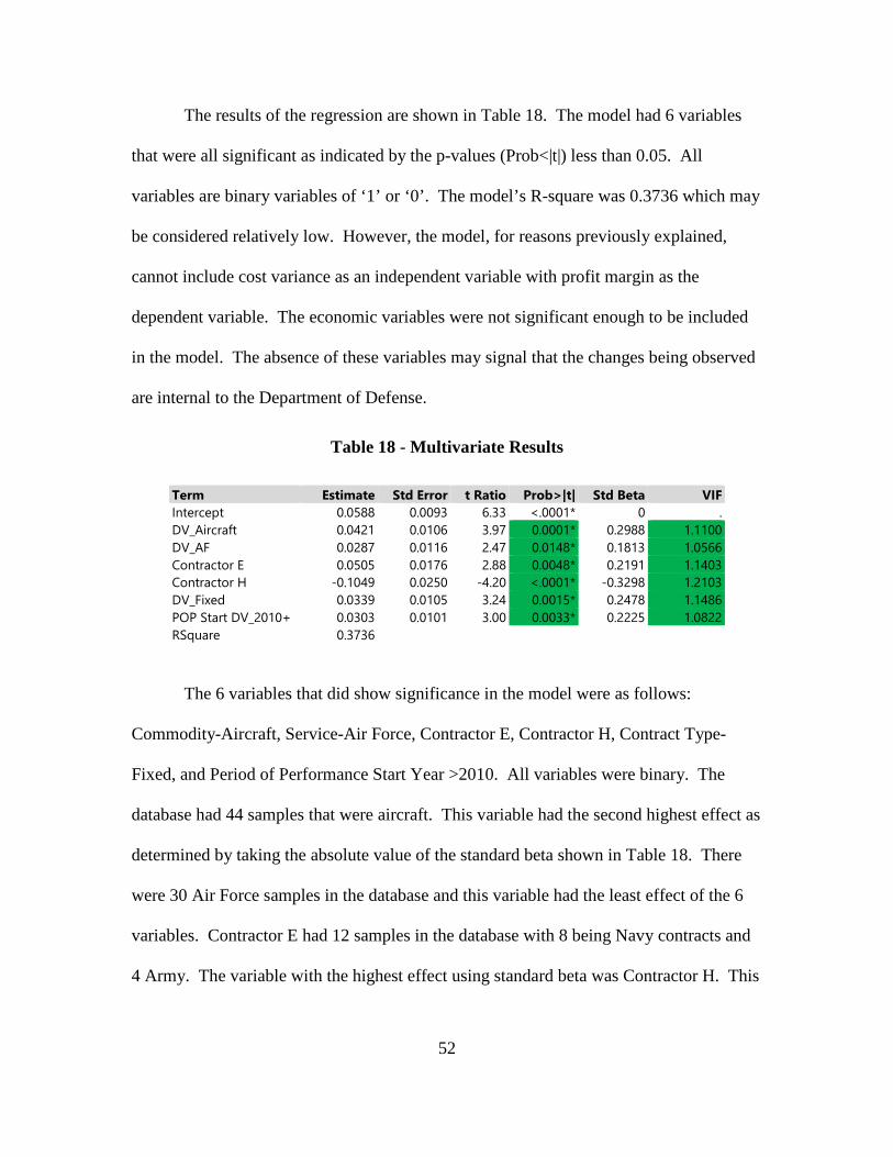
52

The results of the regression are shown in Table 18. The model had 6 variables

that were all significant as indicated by the p-values (Prob<|t|) less than 0.05. All

variables are binary variables of ‘1’ or ‘0’. The model’s R-square was 0.3736 which may

be considered relatively low. However, the model, for reasons previously explained,

cannot include cost variance as an independent variable with profit margin as the

dependent variable. The economic variables were not significant enough to be included

in the model. The absence of these variables may signal that the changes being observed

are internal to the Department of Defense.

Table 18 - Multivariate Results

Term Estimate Std Error t Ratio Prob>|t| Std Beta VIF Intercept 0.0588 0.0093 6.33 <.0001* 0 . DV_Aircraft 0.0421 0.0106 3.97 0.0001* 0.2988 1.1100 DV_AF 0.0287 0.0116 2.47 0.0148* 0.1813 1.0566 Contractor E 0.0505 0.0176 2.88 0.0048* 0.2191 1.1403 Contractor H -0.1049 0.0250 -4.20 <.0001* -0.3298 1.2103 DV_Fixed 0.0339 0.0105 3.24 0.0015* 0.2478 1.1486 POP Start DV_2010+ 0.0303 0.0101 3.00 0.0033* 0.2225 1.0822 RSquare 0.3736

The 6 variables that did show significance in the model were as follows:

Commodity-Aircraft, Service-Air Force, Contractor E, Contractor H, Contract Type-

Fixed, and Period of Performance Start Year >2010. All variables were binary. The

database had 44 samples that were aircraft. This variable had the second highest effect as

determined by taking the absolute value of the standard beta shown in Table 18. There

were 30 Air Force samples in the database and this variable had the least effect of the 6

variables. Contractor E had 12 samples in the database with 8 being Navy contracts and

4 Army. The variable with the highest effect using standard beta was Contractor H. This

53

contractor experienced poor performance on 6 samples. However, 5 of the 6 samples

were all for the same Navy program. Each report was for performance on different

periods of the project. Next, the variable for fixed contract type was significant in the

model. There were 51 fixed samples which were 68% Navy. These 51 samples were

mostly commodities of aircraft or ships. Fixed type contracts would be expected to earn

more profit than cost contracts as fixed contracts contain more risk for the contractor.

Lastly, the variable distinguishing between pre-2011 and post-2010 was significant.

There were 52 samples post-2010 in which 31% of these were aircraft and 52% were

Navy. The results were then tested for normality, constant variance, multi-collinearity,

outliers, and any other overly influential data points.

The test for normality was completed using a Shapiro-Wilk Test on the residuals

from the Table 18 model. This test used the following hypothesis:

• Ho: Residuals are Normally Distributed

• Ha: NOT normal

The goodness-of-fit test for normality resulted in a p-value of 0.0253 which leads to the

null hypothesis being rejected. However, the shape of the plotted distribution of the

residuals must also be considered before rejecting (Figure 6). The shape of the

distribution could be considered to be “approximately normal”; therefore, the test for

normality would be a “soft-fail” and the analysis could continue.

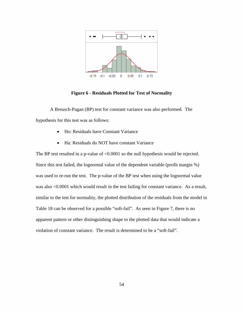
54

Figure 6 - Residuals Plotted for Test of Normality

A Breusch-Pagan (BP) test for constant variance was also performed. The

hypothesis for this test was as follows:

• Ho: Residuals have Constant Variance

• Ha: Residuals do NOT have constant Variance

The BP test resulted in a p-value of <0.0001 so the null hypothesis would be rejected.

Since this test failed, the lognormal value of the dependent variable (profit margin %)

was used to re-run the test. The p-value of the BP test when using the lognormal value

was also <0.0001 which would result in the test failing for constant variance. As a result,

similar to the test for normality, the plotted distribution of the residuals from the model in

Table 18 can be observed for a possible “soft-fail”. As seen in Figure 7, there is no

apparent pattern or other distinguishing shape to the plotted data that would indicate a

violation of constant variance. The result is determined to be a “soft-fail”.

55

Figure 7 - Residuals by Predicted Plot for Constant Variance

The test for multi-collinearity was accomplished using variance inflation factors

(VIF). VIF is the relation of the variance in a multivariate model divided by the variance

of a bivariate model. Table 18 shows the VIF scores for each variable. Generally, any

VIF score greater than 5.0 would require further analysis as multi-collinearity may be an

issue. None of the variables in the current research have concerns for multi-collinearity.

Next, the impact of any potential outliers was examined by plotting the model’s

studentized residuals. There were two data points that exceeded 3 standard deviations.

These samples were excluded and the model was re-analyzed without them. This

resulted in the dummy variable for Air Force no longer being significant. The two data

points were added back into the model and the variable for Air Force was removed. The

updated model is reflect in Table 19.

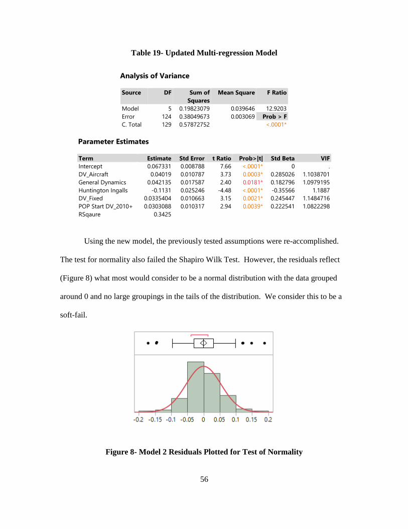
56

Table 19- Updated Multi-regression Model

Analysis of Variance

Source DF Sum of Squares

Mean Square F Ratio

Model 5 0.19823079 0.039646 12.9203 Error 124 0.38049673 0.003069 Prob > F C. Total 129 0.57872752 <.0001*

Parameter Estimates

Term Estimate Std Error t Ratio Prob>|t| Std Beta VIF Intercept 0.067331 0.008788 7.66 <.0001* 0 . DV_Aircraft 0.04019 0.010787 3.73 0.0003* 0.285026 1.1038701 General Dynamics 0.042135 0.017587 2.40 0.0181* 0.182796 1.0979195 Huntington Ingalls -0.1131 0.025246 -4.48 <.0001* -0.35566 1.1887 DV_Fixed 0.0335404 0.010663 3.15 0.0021* 0.245447 1.1484716 POP Start DV_2010+ 0.0303088 0.010317 2.94 0.0039* 0.222541 1.0822298 RSqaure 0.3425

Using the new model, the previously tested assumptions were re-accomplished.

The test for normality also failed the Shapiro Wilk Test. However, the residuals reflect

(Figure 8) what most would consider to be a normal distribution with the data grouped

around 0 and no large groupings in the tails of the distribution. We consider this to be a

soft-fail.

Figure 8- Model 2 Residuals Plotted for Test of Normality

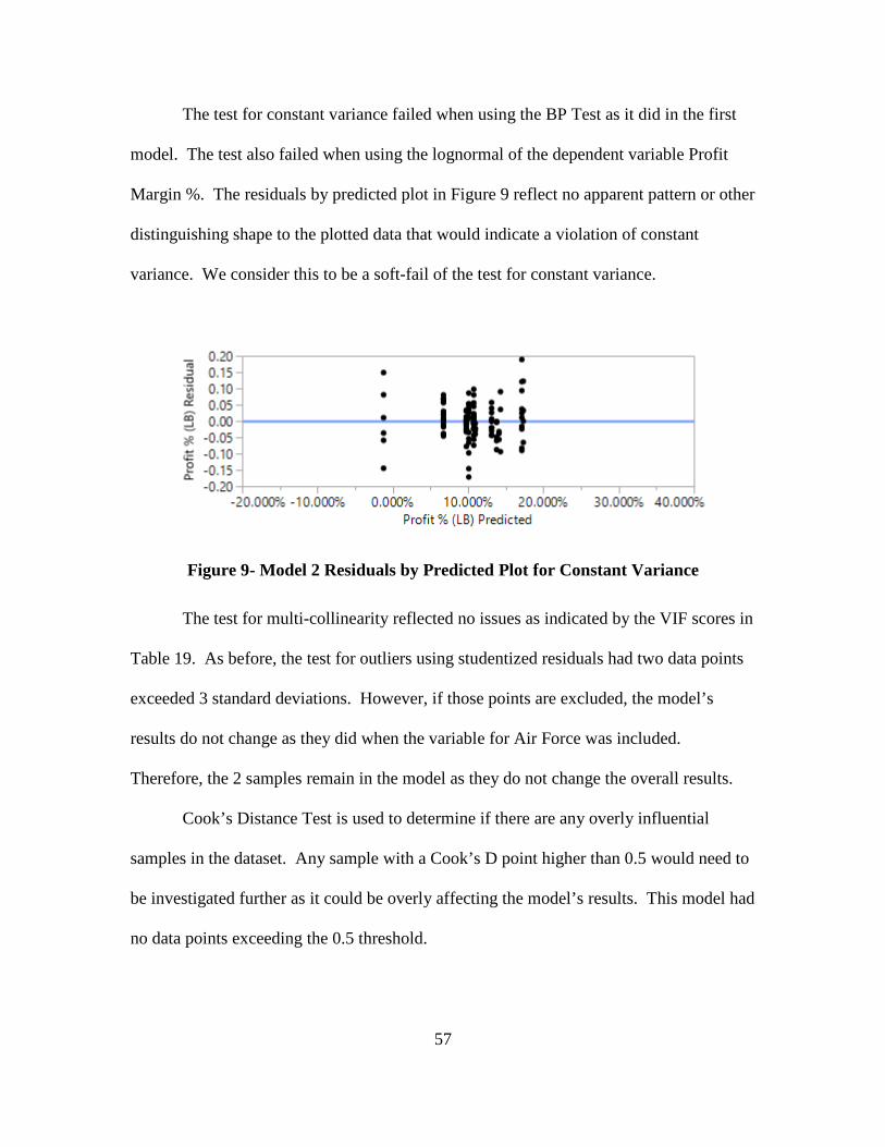
57

The test for constant variance failed when using the BP Test as it did in the first

model. The test also failed when using the lognormal of the dependent variable Profit

Margin %. The residuals by predicted plot in Figure 9 reflect no apparent pattern or other

distinguishing shape to the plotted data that would indicate a violation of constant

variance. We consider this to be a soft-fail of the test for constant variance.

Figure 9- Model 2 Residuals by Predicted Plot for Constant Variance

The test for multi-collinearity reflected no issues as indicated by the VIF scores in

Table 19. As before, the test for outliers using studentized residuals had two data points

exceeded 3 standard deviations. However, if those points are excluded, the model’s

results do not change as they did when the variable for Air Force was included.

Therefore, the 2 samples remain in the model as they do not change the overall results.

Cook’s Distance Test is used to determine if there are any overly influential

samples in the dataset. Any sample with a Cook’s D point higher than 0.5 would need to

be investigated further as it could be overly affecting the model’s results. This model had

no data points exceeding the 0.5 threshold.

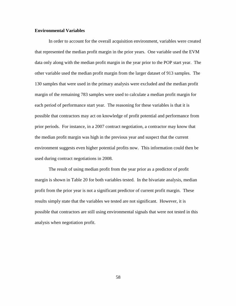
58

Environmental Variables

In order to account for the overall acquisition environment, variables were created

that represented the median profit margin in the prior years. One variable used the EVM

data only along with the median profit margin in the year prior to the POP start year. The

other variable used the median profit margin from the larger dataset of 913 samples. The

130 samples that were used in the primary analysis were excluded and the median profit

margin of the remaining 783 samples were used to calculate a median profit margin for

each period of performance start year. The reasoning for these variables is that it is

possible that contractors may act on knowledge of profit potential and performance from

prior periods. For instance, in a 2007 contract negotiation, a contractor may know that

the median profit margin was high in the previous year and suspect that the current

environment suggests even higher potential profits now. This information could then be

used during contract negotiations in 2008.

The result of using median profit from the year prior as a predictor of profit

margin is shown in Table 20 for both variables tested. In the bivariate analysis, median

profit from the prior year is not a significant predictor of current profit margin. These

results simply state that the variables we tested are not significant. However, it is

possible that contractors are still using environmental signals that were not tested in this

analysis when negotiation profit.

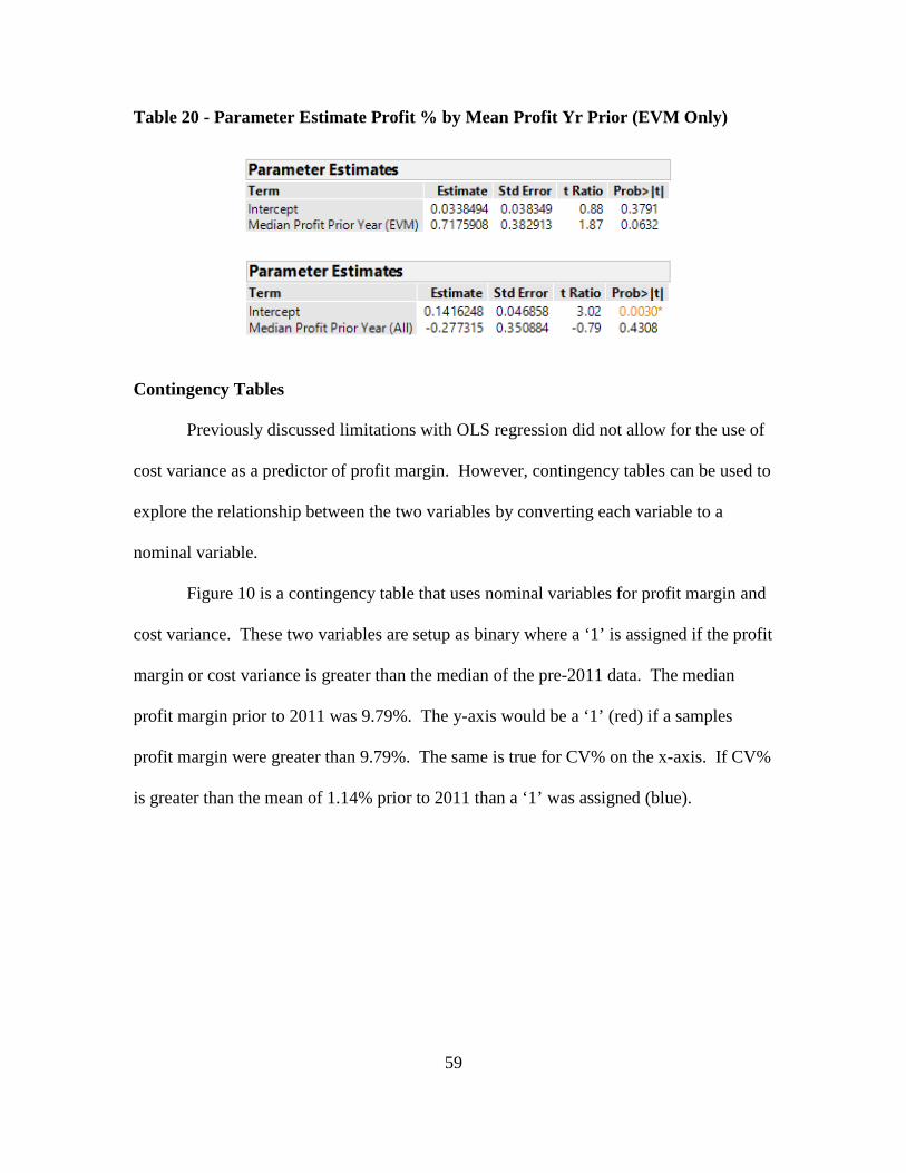
59

Table 20 - Parameter Estimate Profit % by Mean Profit Yr Prior (EVM Only)

Contingency Tables

Previously discussed limitations with OLS regression did not allow for the use of

cost variance as a predictor of profit margin. However, contingency tables can be used to

explore the relationship between the two variables by converting each variable to a

nominal variable.

Figure 10 is a contingency table that uses nominal variables for profit margin and

cost variance. These two variables are setup as binary where a ‘1’ is assigned if the profit

margin or cost variance is greater than the median of the pre-2011 data. The median

profit margin prior to 2011 was 9.79%. The y-axis would be a ‘1’ (red) if a samples

profit margin were greater than 9.79%. The same is true for CV% on the x-axis. If CV%

is greater than the mean of 1.14% prior to 2011 than a ‘1’ was assigned (blue).

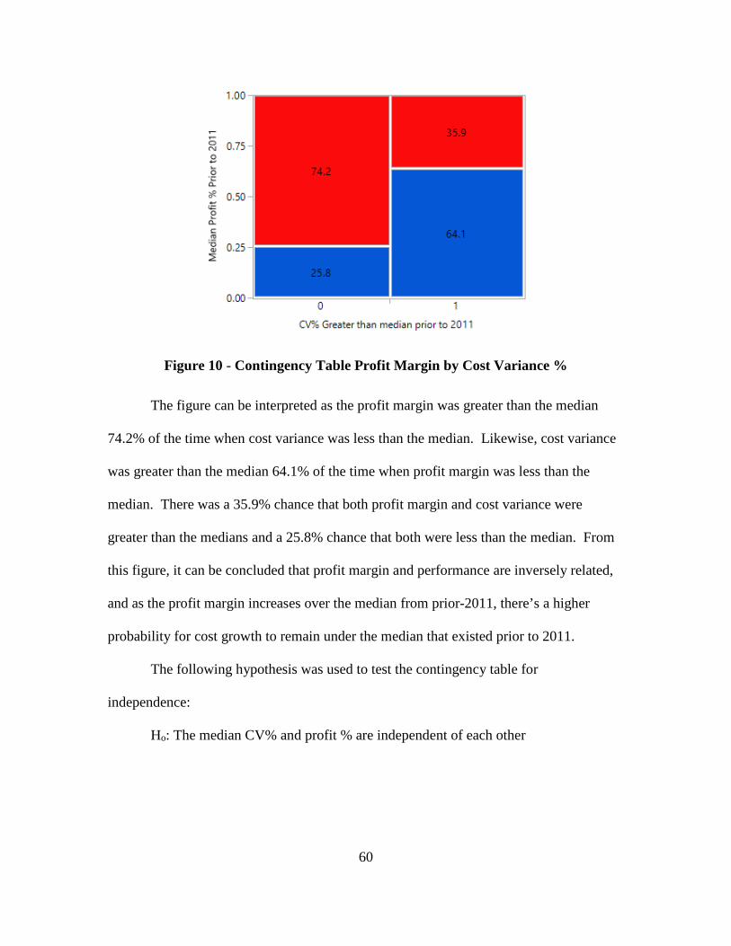
60

Figure 10 - Contingency Table Profit Margin by Cost Variance %

The figure can be interpreted as the profit margin was greater than the median

74.2% of the time when cost variance was less than the median. Likewise, cost variance

was greater than the median 64.1% of the time when profit margin was less than the

median. There was a 35.9% chance that both profit margin and cost variance were

greater than the medians and a 25.8% chance that both were less than the median. From

this figure, it can be concluded that profit margin and performance are inversely related,

and as the profit margin increases over the median from prior-2011, there’s a higher

probability for cost growth to remain under the median that existed prior to 2011.

The following hypothesis was used to test the contingency table for

independence:

Ho: The median CV% and profit % are independent of each other

61

Ha: The probability (sample profit margin > than the median profit margin prior to

2011) is greater when the observed CV% is less than the median CV% prior to

2011

The Fisher’s Exact Test resulted in a p-value of <0.0001 for the left-tailed test.

Since this value was less than 0.05, the null hypothesis is rejected. This signals that the

two variables are dependent of each other and that the likelihood of profit margin

exceeding 9.79% is more probable when the cost variance is less than 1.14%.

Sensitivity Analysis

It may be contested that the chosen year of 2010 captures an effect that would be

found by choosing another year. That is a concern for the study, and a sensitivity

analysis was conducted using the year 2008 as a dividing year. This sensitivity analysis

will assist in answering the final research question which revolves around the degree in

which we can relate profit and performance to overall policy and program aspects.

First, the sensitivity analysis used the non-parametric Wilcoxon Test to test for

significant difference in medians for both profit margin and cost variance during the pre-

2009 period and post-2008 period. When using profit margin as the dependent variable,

the p-value was 0.0224 indicating the medians were significantly different. When using

cost variance as the dependent variable, the medians were also significantly different with

a p-value of 0.0261.

Next, similar to what was accomplished earlier in chapter 4, the difference in IF

and Non-IF contracts during the pre-2009 and post-2008 period was analyzed for both

profit and cost variance. These results are shown in Table 21. For easier reference, the

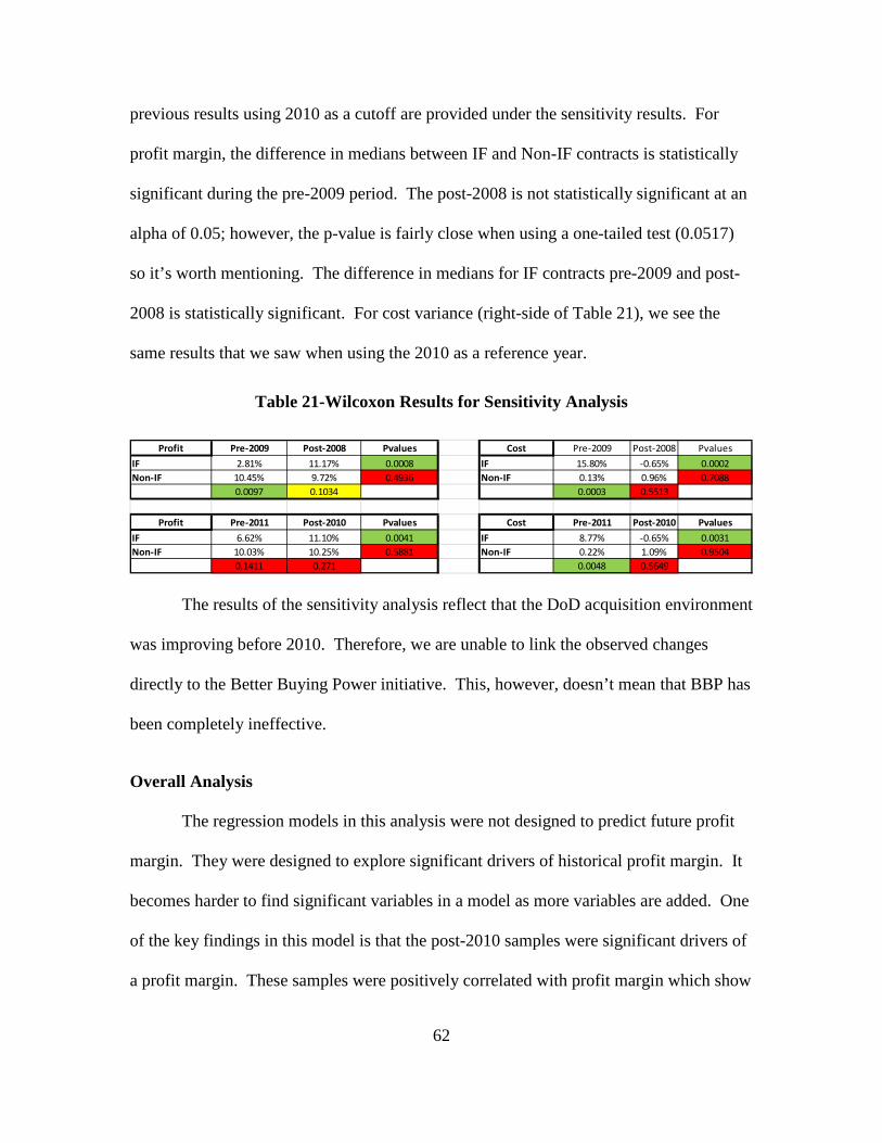
62

previous results using 2010 as a cutoff are provided under the sensitivity results. For

profit margin, the difference in medians between IF and Non-IF contracts is statistically

significant during the pre-2009 period. The post-2008 is not statistically significant at an

alpha of 0.05; however, the p-value is fairly close when using a one-tailed test (0.0517)

so it’s worth mentioning. The difference in medians for IF contracts pre-2009 and post-

2008 is statistically significant. For cost variance (right-side of Table 21), we see the

same results that we saw when using the 2010 as a reference year.

Table 21-Wilcoxon Results for Sensitivity Analysis

The results of the sensitivity analysis reflect that the DoD acquisition environment

was improving before 2010. Therefore, we are unable to link the observed changes

directly to the Better Buying Power initiative. This, however, doesn’t mean that BBP has

been completely ineffective.

Overall Analysis

The regression models in this analysis were not designed to predict future profit

margin. They were designed to explore significant drivers of historical profit margin. It

becomes harder to find significant variables in a model as more variables are added. One

of the key findings in this model is that the post-2010 samples were significant drivers of

a profit margin. These samples were positively correlated with profit margin which show

Profit Pre-2009 Post-2008 Pvalues Cost Pre-2009 Post-2008 PvaluesIF 2.81% 11.17% 0.0008 IF 15.80% -0.65% 0.0002Non-IF 10.45% 9.72% 0.4936 Non-IF 0.13% 0.96% 0.7088

0.0097 0.1034 0.0003 0.5513

Profit Pre-2011 Post-2010 Pvalues Cost Pre-2011 Post-2010 PvaluesIF 6.62% 11.10% 0.0041 IF 8.77% -0.65% 0.0031Non-IF 10.03% 10.25% 0.5881 Non-IF 0.22% 1.09% 0.9504

0.1411 0.271 0.0048 0.5649

63

that something happened in the year’s post-2010 where profit margins increased. None

of the economic or environmental variables that were discussed proved to be significant

in the multi-regression model. The absence of these control variables may indicate that

the acquisition changes were internal to the DOD and not the general public.

Using the presented data, there may be evidence to support the Better Buying

Power reform and its impact on improving the acquisition community. Cost growth has

declined between the pre-2011 and post-2010 period and profit margins have increased

over the same periods. However, the sensitivity analysis findings reflect changes

occurring prior to the BBP implementation. This finding makes it difficult to determine

exactly to what degree the observed changes are attributable to BBP.

64

V. Conclusions and Recommendations

Chapter Overview

The research questions presented in Chapter 1 are reviewed, and interpreted

answers are provided using the results from Chapter 4. Next, limitations in the data and

research methods are discussed. Finally, recommendations for future research are

presented.

Conclusion of Research

The first research question in this analysis examined what trends of profit margin

and cost growth are observed over time. Cost variance and profit margin were plotted as

dependent variables with the period of performance start year as the independent

variable. This resulted in profit margin reflecting a positive correlation with time, such

as, as the years progressed, profit margin increased. Cost variance reflected a negative

correlation. These trends set the framework for the remaining analysis as they are what

we would expect to see if Better Buying Power has been effective.

The research then examined specific trends relative to when BBP was initiated in

2010. First, the research found a statistically significant difference in medians for both

profit margin and cost variance from before 2011 and after 2010. The median profit

margin prior to 2011 was 9.79% and the mean cost variance was 1.14%. For the period

post-2010, the median profit margin increased to 10.91% and the mean cost variance

declined to 0.33%.

In addition, BBP recommended using incentive structured (IF) over award fee

(AF) structured contracts. This report showed that there was an increased usage of

65

incentive structures and a reduced use of the award structure. For the incentive structured

samples, profit margin increased from 6.62% before 2011 to 11.10% after 2010.

Likewise, the cost growth for the IF samples declined from 8.77% to -0.65%. The non-

parametric Wilcoxon Test confirmed that these differences were statistically significant.

These results may signal that the DoD has embraced the mentality of Chao (2013) who

implied we ought not shy away from profits, but treat them as a rightful reward for

performance. Perhaps the DoD is now willing to pay higher profit in exchange for better

contract performance. In addition, the results may indicate that acquisition professionals

are adhering to recommendations and guidance that Better Buying Power has introduced.

Lastly, the third research question looked to determine the degree in which

observed changes are attributable to the larger economy, program aspects, and overall

policy. Multivariate regression was one tool used to assist in answering this question by

finding a model that best represented the profit data. There were no variables that were

highly predictive of profit margin. The multivariate model was only able to explain 34%

of the variance in the mean profit margin. While the results are naturally tempered by the

inability to include performance into the OLS regression, this result signals that there is

still a large amount of variance to be explained which is logical as there is only so much

that can be controlled through incentives. Importantly, the research found that economic

factors such as unemployment rate, federal funds rate, gross domestic product (GDP),

and the branch of service’s budget were not significant predictors of profit margin. This

suggests that the underlying reason for the observed trends may be internal to the DoD

through technical differences in programs or management of programs. In addition, there

was little evidence to support that the changes being observed were due to the overall

66

acquisition environment. The environmental variables were exploratory and found no

significant results. This does not convey that the environment has not had an impact but

simply means additional exploration may be necessary.

Cost growth is believed to be a major predictor of profit margin. However,

performance, in the form of cost growth, was one variable that was not able to be tested

as an independent variable with profit margin as a dependent variable. Therefore,

contingency tables were used to show a dependent relationship between profit margin and

cost variance where profit margin increases as cost variance declines and vice versa.

A central question of the research was to determine how (if at all) Better Buying

Power had impacted the DoD acquisition community. It is more difficult to determine,

however, if the changes observed may be traced specifically to the implementation of

BBP. This study found the trends to have begun before 2010 as seen through the

sensitivity analysis which produced statistically significant differences when using other

years.

The study has, nonetheless, identified a pattern which should give some faith that

the environment set by a series of acquisition reforms has improved its management of

cost. There has been a marked reduction in cost overruns in recent years. This study’s

preliminary analysis of economic variables found no dramatic changes attributable to the

economy which seems to indicate changes are due to contractor performance.

Limitations

The current research had a few significant limitations. First, the dataset used in

this analysis was a combination of two different data sources. Profit data was pulled

67

from Cost Data Summary Reports (CDSR) and performance data from Earned Value

Management (EVM) reports. Not all projects require EVM reporting. Therefore, there

were significantly more CDSR reports available than there were EVM reports. Each of

these reports have their owned intended purposes and are not designed to be easily

compared with each other. As such, linking CDSR samples to EVM samples was a

complicated process. Second, one of the unique aspects of this research was analyzing

profit and performance. However, as discussed in Chapter 3, these two variables were

not able to be analyzed using regression. Consequently, other predictors of profit margin

were explored using statistical analysis. Lastly, the current research was focused on the

changes that occurred before and after Better Buying Power was initiated. Most projects

in the database have periods of performance that are several years in length. Therefore,

the sample size of the analysis was limited as many projects starting after 2014 are still in

progress.

Recommendations for Future Research

There is ample opportunity for future research on topics similar to those presented

in the current research. The current study has shown a marked uptick in the use of

incentive contracts, but such growth cannot continue indefinitely. It will be interesting to

see how cost performance changes with an expanded time frame, and once an equilibrium

or new norm is established. While this study finds the new trends encouraging, it is

possible that the momentum toward incentive contracts goes too far, pushing into

contract areas where it is ill-suited. In many ways, the current study was an early look at

a dynamic that yet to full play out. First, as time progresses, there should be more data

68

available to compare pre-2011 and post-2010. In addition, the effect of the other Better

Buying Power initiatives in 2012 and 2015 could also be examined. This analysis could

introduce contractor performance ratings from the Contractor Performance Assessment

Reporting System (CPARS) to create a more robust analysis. Second, further research

could also be done on profit margin in the form examining specific contract profits and

contractual profit share ratios. Lastly, the environment of the DoD acquisition

community has much to explore. Training initiatives and certification requirements have

changed drastically in the past decade. Research on the effect of this training and

certification requirement could be accomplished to determine if positive changes in

recent years are attributable to the workforce becoming better at their jobs.

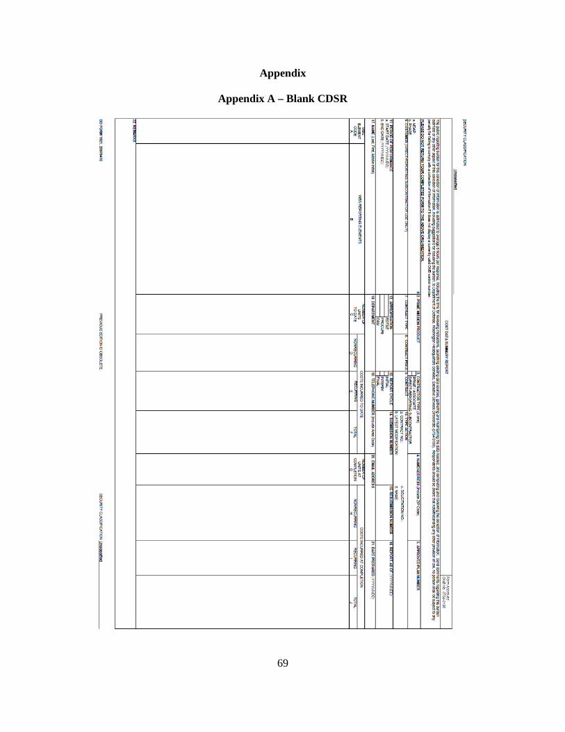
69

Appendix

Appendix A – Blank CDSR

70

Appendix B - Cost and Software Data Reporting (CSDR) Requirements

Source: DoDI 5000.02

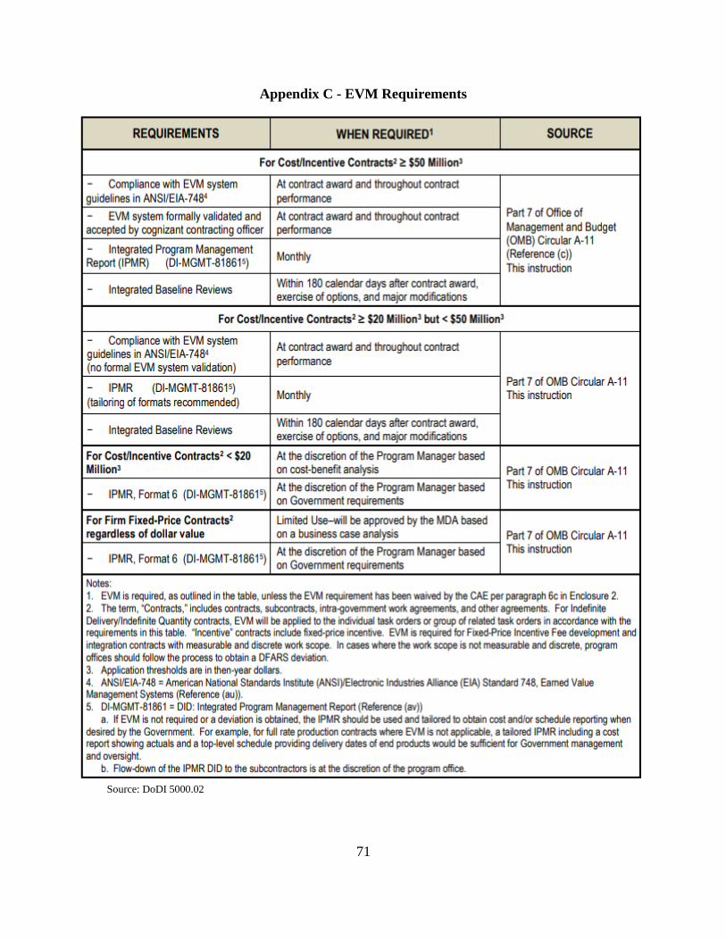
71

Appendix C - EVM Requirements

Source: DoDI 5000.02

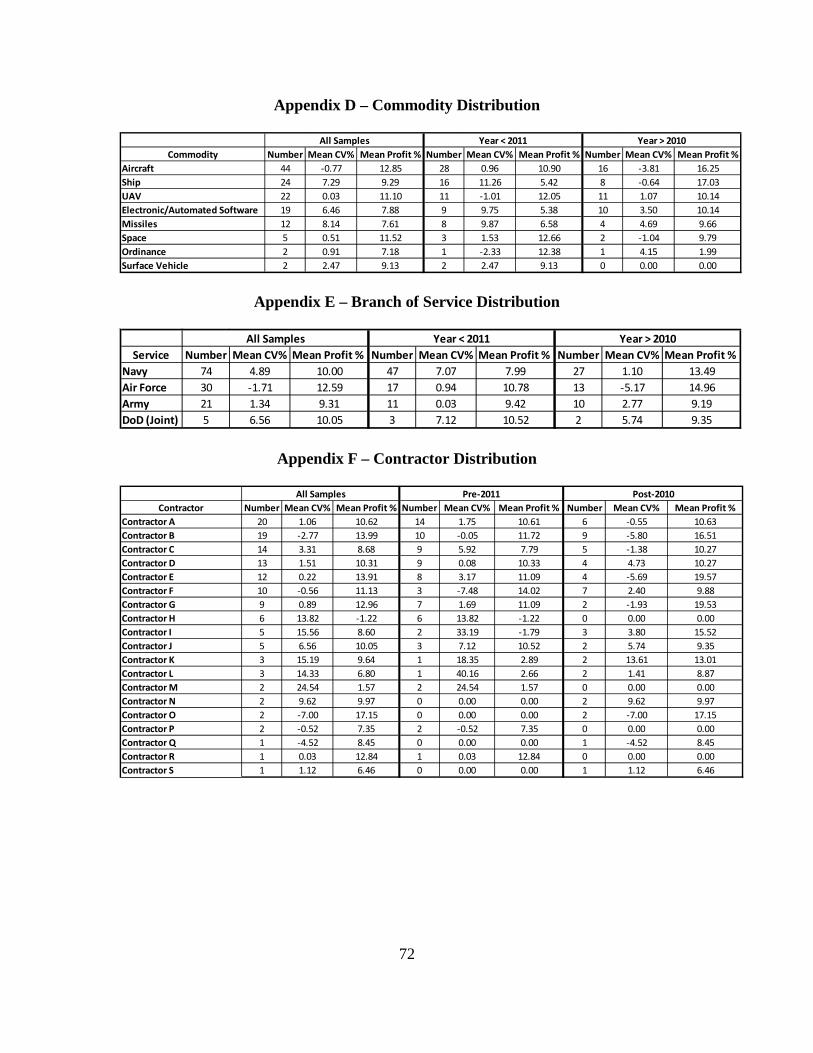
72

Appendix D – Commodity Distribution

Appendix E – Branch of Service Distribution

Appendix F – Contractor Distribution

Commodity Number Mean CV% Mean Profit % Number Mean CV% Mean Profit % Number Mean CV% Mean Profit %Aircraft 44 -0.77 12.85 28 0.96 10.90 16 -3.81 16.25Ship 24 7.29 9.29 16 11.26 5.42 8 -0.64 17.03UAV 22 0.03 11.10 11 -1.01 12.05 11 1.07 10.14Electronic/Automated Software 19 6.46 7.88 9 9.75 5.38 10 3.50 10.14Missiles 12 8.14 7.61 8 9.87 6.58 4 4.69 9.66Space 5 0.51 11.52 3 1.53 12.66 2 -1.04 9.79Ordinance 2 0.91 7.18 1 -2.33 12.38 1 4.15 1.99Surface Vehicle 2 2.47 9.13 2 2.47 9.13 0 0.00 0.00

All Samples Year < 2011 Year > 2010

Service Number Mean CV% Mean Profit % Number Mean CV% Mean Profit % Number Mean CV% Mean Profit %Navy 74 4.89 10.00 47 7.07 7.99 27 1.10 13.49Air Force 30 -1.71 12.59 17 0.94 10.78 13 -5.17 14.96Army 21 1.34 9.31 11 0.03 9.42 10 2.77 9.19DoD (Joint) 5 6.56 10.05 3 7.12 10.52 2 5.74 9.35

Year < 2011 Year > 2010All Samples

Contractor Number Mean CV% Mean Profit % Number Mean CV% Mean Profit % Number Mean CV% Mean Profit %Contractor A 20 1.06 10.62 14 1.75 10.61 6 -0.55 10.63Contractor B 19 -2.77 13.99 10 -0.05 11.72 9 -5.80 16.51Contractor C 14 3.31 8.68 9 5.92 7.79 5 -1.38 10.27Contractor D 13 1.51 10.31 9 0.08 10.33 4 4.73 10.27Contractor E 12 0.22 13.91 8 3.17 11.09 4 -5.69 19.57Contractor F 10 -0.56 11.13 3 -7.48 14.02 7 2.40 9.88Contractor G 9 0.89 12.96 7 1.69 11.09 2 -1.93 19.53Contractor H 6 13.82 -1.22 6 13.82 -1.22 0 0.00 0.00Contractor I 5 15.56 8.60 2 33.19 -1.79 3 3.80 15.52Contractor J 5 6.56 10.05 3 7.12 10.52 2 5.74 9.35Contractor K 3 15.19 9.64 1 18.35 2.89 2 13.61 13.01Contractor L 3 14.33 6.80 1 40.16 2.66 2 1.41 8.87Contractor M 2 24.54 1.57 2 24.54 1.57 0 0.00 0.00Contractor N 2 9.62 9.97 0 0.00 0.00 2 9.62 9.97Contractor O 2 -7.00 17.15 0 0.00 0.00 2 -7.00 17.15Contractor P 2 -0.52 7.35 2 -0.52 7.35 0 0.00 0.00Contractor Q 1 -4.52 8.45 0 0.00 0.00 1 -4.52 8.45Contractor R 1 0.03 12.84 1 0.03 12.84 0 0.00 0.00Contractor S 1 1.12 6.46 0 0.00 0.00 1 1.12 6.46

All Samples Pre-2011 Post-2010

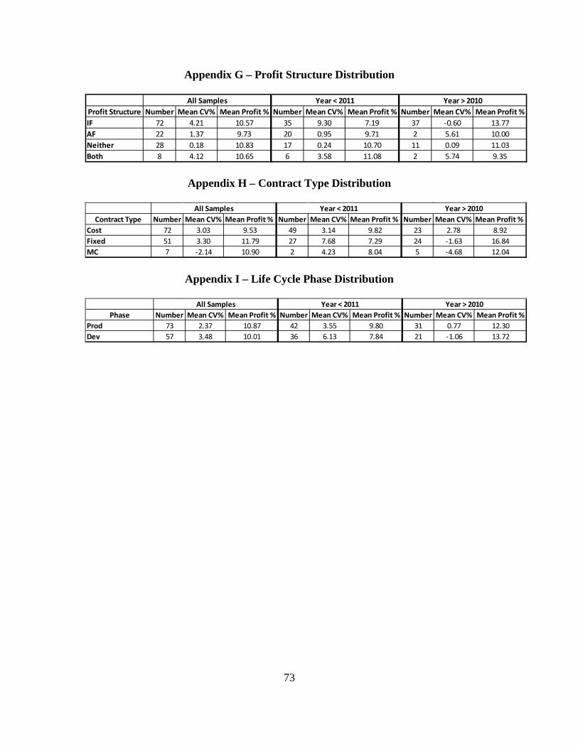
73

Appendix G – Profit Structure Distribution

Appendix H – Contract Type Distribution

Appendix I – Life Cycle Phase Distribution

Profit Structure Number Mean CV% Mean Profit % Number Mean CV% Mean Profit % Number Mean CV% Mean Profit %IF 72 4.21 10.57 35 9.30 7.19 37 -0.60 13.77AF 22 1.37 9.73 20 0.95 9.71 2 5.61 10.00Neither 28 0.18 10.83 17 0.24 10.70 11 0.09 11.03Both 8 4.12 10.65 6 3.58 11.08 2 5.74 9.35


Contract Type Number Mean CV% Mean Profit % Number Mean CV% Mean Profit % Number Mean CV% Mean Profit %Cost 72 3.03 9.53 49 3.14 9.82 23 2.78 8.92Fixed 51 3.30 11.79 27 7.68 7.29 24 -1.63 16.84MC 7 -2.14 10.90 2 4.23 8.04 5 -4.68 12.04


Phase Number Mean CV% Mean Profit % Number Mean CV% Mean Profit % Number Mean CV% Mean Profit %Prod 73 2.37 10.87 42 3.55 9.80 31 0.77 12.30Dev 57 3.48 10.01 36 6.13 7.84 21 -1.06 13.72


74

Bibliography

Abate, C.C. (2004), An Analysis of Missile Systems Cost Growth and Implementation of Acquisition Reform Initiatives Using a Hybrid Adjusted Cost Growth Model, MS Thesis, School of Engineering and Management, Air Force Institute of Technology, Wright-Patterson AFB: OH.

Agresti, A. (1992). A survey of exact inference for contingency tables. Statistical Science, 7(1), 131-177.

Arena, M.V., Leonard, R.S., Murray, S.E., and Younossi, O. (2006), Historical Cost Growth of Completed Weapon System Programs, Santa Monica, CA: RAND Corporation.

Arnold, S. A., Harmon, B. R., Tyson, K. W., Fasana, K. G., & Wait, C. S. (2008). Defense Department Profit and Contract Finance Policies and Their Effects on Contract and Contractor Performance (No. IDA-P-4284). Institute for Defense Analyses Alexandria Va.

Berteau, D., Hofbauer, J., & Sanok, S. (2010). Implementation of the Weapon Systems Acquisition Reform Act of 2009: A progress report. Washington, DC: Center for Strategic and International Studies.

Better Buying Power 2.0. (2013). Retrieved July 21, 2018, from

https://www.acq.osd.mil/fo/docs/USD(AT&L)%20BBP%202.0%20Implementation%20Directive%20(24%20April%202013).pdf

Better Buying Power 3.0. (2015). Retrieved July 21, 2018, from https://www.acq.osd.mil/fo/docs/betterBuyingPower3.0(9Apr15).pdf

Biery, F.P. (1992), The Effectiveness of Weapon System Acquisition Reform Efforts, Journal of Policy Analysis and Management, Vol. 11, 4: 637-664.

Buchanan, J.M. (1979), “Politics without Romance: A Sketch of Positive Public Choice Theory and Its Normative Implications”, in The Collected Works of James M. Buchanan, Vol 1, Liberty Fund, Indianapolis, IN, 1999.

Buchanan, J.M. et al. (1978). The Economics of Politics, Institute of Economic Affairs, London, pg 1-20.

CADE. (n.d.). Retrieved from http://cade.osd.mil/(S(ttctvqv3k2ppcizbrrgs2yss))/about/cade

CAPE. (2018, February). FY 2016 Annual Report on Cost Assessment Activities.

Retrieved from https://www.cape.osd.mil/files/Reports/CA_AR_2016.pdf

75

Chaplain, C. T., Bothwell, B., Campbell, G., Chan, J., Echard, J., Gallegos, A., ... & McGinty, S. (2006). Space Acquisitions: DOD Needs to Take More Action to Address Unrealistic Initial Cost Estimates of Space Systems (No. GAO-07-96). Government Accountability Office. Washington DC.

Choi, D.I. (2009), A Study on Improving Defense Acquisition Through the Application of Defense Acquisition Workforce Improvement Act (DAWIA) Concept to Defense Industry Workforce, MS Thesis, Naval Postgraduate School, Monterey: CA.

Christensen, D. S., Searle, D. A., and Vickery, C. (1999), “The Impact of the Packard Commission‘s Recommendations on Reducing Cost Overruns on Defense Acquisition Contracts”, Acquisition Review Quarterly, Summer.

Cross, J. (1966). A reappraisal of cost incentives in defense contracts (No. RP-P-282). Institute For Defense Analyses. Alexandria Va Economic And Political Studies Div.

Data item description “Cost Data Summary Report” (DD Form 1921). (2011). Retrieved from http://cade.osd.mil/content/cade/files/csdr/dids/current/1921.DI-FNCL-81565C.pdf

Davis, D., & Anton, P. S. (2016). Annual Growth of Contract Costs for Major Programs in Development and Early Production. Office of the Under Secretary of Defense for Acquisition, Technology, and Logistics Washington United States.

Defense Acquisition Performance Assessment (2005), ‘A Report by the Panel of the Defense Acquisition Performance Assessment Project’, December 2005.

Drezner, J. A., & Smith, G. K. (1990). An Analysis of Weapon System Acquisition Schedules, Santa Monica, CA: RAND Corporation.

Drezner, J.A, Jarvaise, J.M., Hess, R., Norton, D.M., and Hough, P.G. (1993), An Analysis of Weapon System Cost Growth, Santa Monica, CA: RAND Corporation.

Fisher, I. N. (1968). A Reappraisal Of Incentive Contracting Experience (No. RAND-M-5700-PR). RAND Corp Santa Monica CA.

Flyvbjerg, B., Bruzelius, N., & Rothengatter, W. (2003). Megaprojects and Risk: An Anatomy of Ambition. Cambridge University Press.

Frazier, T. P., Cloos, J. J., & Kimko, D. (2001) “Cost Sharing Arrangements on Incentive Contracts,” briefing slides.

Garcia, A., Keyner, H., Robillard, T.J., and VanMullekom, M. (1997), “The Defense Acquisition Workforce Improvement Act: Five Years Later”, Acquisition Review Quarterly, Summer: 295-314.

76

Gardener, T., & Moffat, J. (2008). Changing Behaviours in Defence Acquisition: A Game Theory Approach. Journal of the Operational Research Society, 59(2), 225-230. doi:10.1057/palgrave.jors.2602476

Government Accountability Office. (1987, March DOD's Profit Policy and GAO's Proposal for a Program To Study the Profitability of Government Contractors. Retrieved August 14, 2018, from https://www.gao.gov/products/T-NSIAD-87-11

Government Accountability Office. (1997). Acquisition Reform: Effect on Weapon System Funding. Retrieved from https://www.gao.gov/products/NSIAD-98-31

Government Accountability Office. (2005, December). Defense Acquisitions: DOD Has Paid Billions in Award and Incentive Fees Regardless of Acquisition Outcomes. Retrieved August 14, 2018, from https://www.gao.gov/new.items/d0666.pdf

Government Accountability Office. (2009, May). Federal Contracting: Guidance on Award Fees Has Led to Better Practices but Is Not Consistently Applied. Retrieved August 14, 2018, from https://www.gao.gov/assets/300/290295.pdf

Government Accountability Office. (2017, July). Defense Contracting: DOD Needs Better Information on Incentive Outcomes. Retrieved August 14, 2018, from https://www.gao.gov/assets/690/685723.pdf

Hanks, C. H., Axelband, E. I., Lindsay, S., Malik, M. R., & Steele, B. D. (2005). Reexamining Military Acquisition Reform: Are We There Yet?, Santa Monica, CA: RAND Corporation.

Holbrook, M. A. (2003), ‘An Analysis of the Implementation of Acquisition Reform Initiatives and Cost Variance’, MS Thesis, School of Engineering and Management, Air Force Institute of Technology, Wright-Patterson AFB: OH.

Kendall, F. (2015). Tying Profit to Performance A Valuable Tool, But Use With Good Judgment.

Lorell, M., & Graser, J. C. (2001). An Overview of Acquisition Reform Cost Savings Estimates, Santa Monica, CA: RAND Corporation.

Nordwall, B.D. (1987), ‘Packard Commission Set to Reconvene’, Aviation Week and Space Technology, 30 March: 80-81.

OUSD(AT&L). (2014). Performance of the Defense Acquisition System, 2014 Annual Report. Retrieved from https://dod.defense.gov/Portals/1/Documents/pubs/Performance-of-Defense-Acquisition-System-2014.pdf

OUSD(AT&L). (2016). Performance of the Defense Acquisition System, 2016 Annual Report. Retrieved from http://www.dtic.mil/docs/citations/AD1019605

77

Paltrow, S. J. (2013, December 23). Special Report: Why the Pentagon's Accounting Fixes End Up Broken. Retrieved from https://www.reuters.com/article/us-usa-pentagon-brokenfixes-specialrepor/special-report-why-the-pentagons-accounting-fixes-end-up-broken-idUKBRE9BM0HM20131223

Phillips, R.A. (2004), ‘An Analysis of Aircraft Weapon System Cost Growth and Implementation of Acquisition Reform Initiatives Using a Hybrid Adjusted Cost Growth Model’, MS Thesis, School of Engineering and Management, Air Force Institute of Technology, Wright-Patterson AFB: OH.

Rhea, A. M. (2017). Comparison of Profit Margin Percentages Between Prime Contractors and Subcontractors for Aircraft, Missiles, and Unmanned Aerial Vehicles (No. AFIT-ENV-MS-17-M-215). Air Force Institute of Technology. Wright-Patterson AFB OH.

Ritschel, J. D. (2011). Political Economy of Military Weapon Systems Acquisitions. George Mason University.

Rogerson, W. (1992). Profit Regulation of Defense Contractors and Prizes for Innovation. Santa Monica, CA: RAND Corporation.

Schecter, S., & Gintis, H. (2016). Game Theory In Action: An Introduction To Classical And Evolutionary Models. Princeton: Princeton University Press.

Schelling, T. C. (1980). The Strategy of Conflict. Harvard university press.

Searle, D.A. (1997), ‗The Impact of the Packard Commission‟s Recommendations on Reducing Cost Overruns in Major Defense Acquisition Programs‟, MS Thesis, Graduate Cost Analysis Masters Program, Air Force Institute of Technology, Wright-Patterson AFB, OH.

Shaw, J. S. (n.d.). Public Choice Theory. Retrieved November 7, 2018, from http://www.econlib.org/library/Enc1/PublicChoiceTheory.html

Shughart, W. F., II. (n.d.). Public Choice. Retrieved November 7, 2018, from https://www.econlib.org/library/Enc/PublicChoice.html

Smirnoff, J.P and M.J. Hicks (2008), ‘The Impact Of Economic Factors And Acquisition Reforms On The Cost Of Defense Weapons Systems‘, Review of Financial Economics, 17, 3-13.

Snider, K.F. (1996), ‘DAWIA and the Price of Professionalism‘, Acquisition Review Quarterly, Fall: 97-108.

Stigler, G. J. (1961). The Economics of Information. Journal of Political Economy, 69(3), 213-225.

78

Tullock, G., Brady, G. L., & Seldon, A. (2002). Government Failure: A Primer in Public Choice. Cato Institute.

Turocy, T. L., & Von Stengel, B. (2001, October 8). Game Theory. Retrieved November 8, 2018, from http://www.cdam.lse.ac.uk/Reports/Files/cdam-2001-09.pdf

Twenty‐five Years of Acquisition Reform: Where Do We Go From Here? (2013) (testimony of Pierre A. Chao).

79

Vita

Captain Jerry “Trey” Baker received his Bachelor of Business Administration in

finance from the University of Memphis in 2011 and commissioned into the Air Force

through Officer Training School in May 2013. He received his Master of Business

Administration from Webster University in 2017.

During his Air Force career, Captain Baker has been a flight commander

responsible for providing financial services to over 12,000 personnel across 3 Wings and

accountable for the budget execution of a $400 million Operations and Maintenance and

Transportation Working Capital Funds budget. In addition, Captain Baker served as the

budget officer, 455th Air Expeditionary Wing, Bagram Air Base, Afghanistan. Upon

graduation from the Air Force Institute of Technology, he will be assigned to the Air

Force Life Cycle Management Center, Wright-Patterson Air Force Base, Ohio.

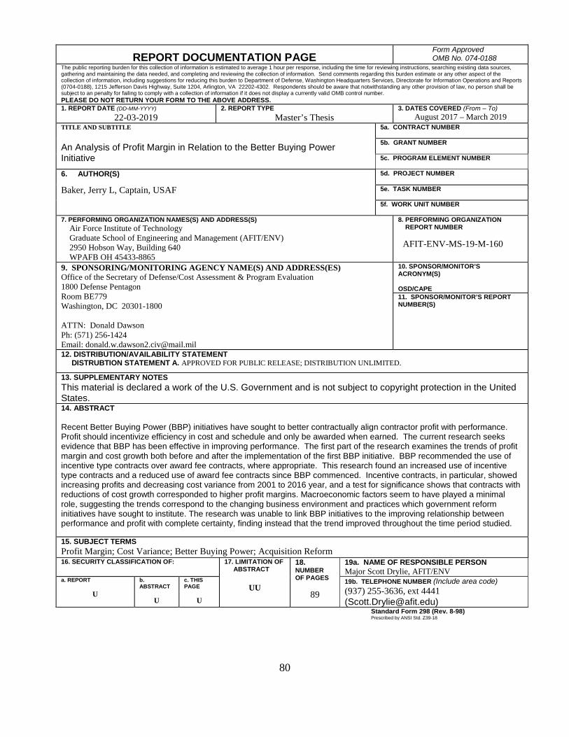
80

REPORT DOCUMENTATION PAGE Form Approved OMB No. 074-0188

The public reporting burden for this collection of information is estimated to average 1 hour per response, including the time for reviewing instructions, searching existing data sources, gathering and maintaining the data needed, and completing and reviewing the collection of information. Send comments regarding this burden estimate or any other aspect of the collection of information, including suggestions for reducing this burden to Department of Defense, Washington Headquarters Services, Directorate for Information Operations and Reports (0704-0188), 1215 Jefferson Davis Highway, Suite 1204, Arlington, VA 22202-4302. Respondents should be aware that notwithstanding any other provision of law, no person shall be subject to an penalty for failing to comply with a collection of information if it does not display a currently valid OMB control number. PLEASE DO NOT RETURN YOUR FORM TO THE ABOVE ADDRESS. 1. REPORT DATE (DD-MM-YYYY)

22-03-2019 2. REPORT TYPE

Master’s Thesis 3. DATES COVERED (From – To)

August 2017 – March 2019 TITLE AND SUBTITLE An Analysis of Profit Margin in Relation to the Better Buying Power Initiative

5a. CONTRACT NUMBER

5b. GRANT NUMBER 5c. PROGRAM ELEMENT NUMBER

6. AUTHOR(S) Baker, Jerry L, Captain, USAF

5d. PROJECT NUMBER 5e. TASK NUMBER

5f. WORK UNIT NUMBER

7. PERFORMING ORGANIZATION NAMES(S) AND ADDRESS(S) Air Force Institute of Technology Graduate School of Engineering and Management (AFIT/ENV) 2950 Hobson Way, Building 640 WPAFB OH 45433-8865

8. PERFORMING ORGANIZATION REPORT NUMBER AFIT-ENV-MS-19-M-160

9. SPONSORING/MONITORING AGENCY NAME(S) AND ADDRESS(ES) Office of the Secretary of Defense/Cost Assessment & Program Evaluation 1800 Defense Pentagon Room BE779 Washington, DC 20301-1800 ATTN: Donald Dawson Ph: (571) 256-1424 Email: [email protected]

10. SPONSOR/MONITOR’S ACRONYM(S) OSD/CAPE 11. SPONSOR/MONITOR’S REPORT NUMBER(S)

12. DISTRIBUTION/AVAILABILITY STATEMENT DISTRUBTION STATEMENT A. APPROVED FOR PUBLIC RELEASE; DISTRIBUTION UNLIMITED.

13. SUPPLEMENTARY NOTES This material is declared a work of the U.S. Government and is not subject to copyright protection in the United States. 14. ABSTRACT Recent Better Buying Power (BBP) initiatives have sought to better contractually align contractor profit with performance. Profit should incentivize efficiency in cost and schedule and only be awarded when earned. The current research seeks evidence that BBP has been effective in improving performance. The first part of the research examines the trends of profit margin and cost growth both before and after the implementation of the first BBP initiative. BBP recommended the use of incentive type contracts over award fee contracts, where appropriate. This research found an increased use of incentive type contracts and a reduced use of award fee contracts since BBP commenced. Incentive contracts, in particular, showed increasing profits and decreasing cost variance from 2001 to 2016 year, and a test for significance shows that contracts with reductions of cost growth corresponded to higher profit margins. Macroeconomic factors seem to have played a minimal role, suggesting the trends correspond to the changing business environment and practices which government reform initiatives have sought to institute. The research was unable to link BBP initiatives to the improving relationship between performance and profit with complete certainty, finding instead that the trend improved throughout the time period studied. 15. SUBJECT TERMS Profit Margin; Cost Variance; Better Buying Power; Acquisition Reform 16. SECURITY CLASSIFICATION OF: 17. LIMITATION OF

ABSTRACT

UU

18. NUMBER OF PAGES

89

19a. NAME OF RESPONSIBLE PERSON Major Scott Drylie, AFIT/ENV

a. REPORT

U

b. ABSTRACT

U

c. THIS PAGE

U

19b. TELEPHONE NUMBER (Include area code) (937) 255-3636, ext 4441 ([email protected])

Standard Form 298 (Rev. 8-98) Prescribed by ANSI Std. Z39-18